Linear Programming
16
9.3 THE SIMPLEX METHOD: MAXIMIZATION For linear programming problems involving two variables, the graphical solution method introduced in Section 9.2 is convenient. However, for problems involving more than two variables or problems involving a large number of constraints, it is better to use solution methods that are adaptable to computers. One such method is called the simplex method, developed by George Dantzig in 1946. It provides us with a systematic way of examining the vertices of the feasible region to determine the optimal value of the objective function. We introduce this method with an example. Suppose we want to find the maximum value of where and subject to the following constraints. Since the left-hand side of each inequality is less than or equal to the right-hand side, there must exist nonnegative numbers and that can be added to the left side of each equa- tion to produce the following system of linear equations. The numbers and are called slack variables because they take up the “slack” in each inequality. s 3 s 1 , s 2 2x 1 1 5x 2 1 s 1 1 s 2 1 s 3 5 90 2x 1 1 5x 2 1 s 1 1 s 2 1 s 3 5 27 2x 1 1 5x 2 1 s 1 1 s 2 1 s 3 5 11 s 3 s 1 , s 2 2x 1 1 5x 2 # 90 2x 1 1 5x 2 # 27 2x 1 1 5x 2 # 11 x 2 $ 0, x 1 $ 0 z 5 4x 1 1 6x 2 , 494 CHAPTER 9 LINEAR PROGRAMMING Standard Form of a Linear Programming Problem A linear programming problem is in standard form if it seeks to maximize the objec- tive function subject to the constraints . . . where and After adding slack variables, the corresponding system of constraint equations is . . . where s i $ 0. a m1 x 1 1 a m2 x 2 1 . . . 1 a mn x n 1 s m 5 b m a 21 x 1 1 a 22 x 2 1 . . . 1 a 2n x n 1 s 2 5 b 2 a 11 x 1 1 a 12 x 2 1 . . . 1 a 1n x n 1 s 1 5 b 1 b i $ 0. x i $ 0 a m1 x 1 1 a m2 x 2 1 . . . 1 a mn x n # b m a 21 x 1 1 a 22 x 2 1 . . . 1 a 2n x n # b 2 a 11 x 1 1 a 12 x 2 1 . . . 1 a 1n x n # b 1 z 5 c 1 x 1 1 c 2 x 2 1 . . . 1 c n x n
-
Upload
sonu-kumar -
Category
Documents
-
view
140 -
download
9
Transcript of Linear Programming

9.3 THE SIMPLEX METHOD: MAXIMIZATIONFor linear programming problems involving two variables, the graphical solution methodintroduced in Section 9.2 is convenient. However, for problems involving more than twovariables or problems involving a large number of constraints, it is better to use solutionmethods that are adaptable to computers. One such method is called the simplex method,developed by George Dantzig in 1946. It provides us with a systematic way of examiningthe vertices of the feasible region to determine the optimal value of the objective function.We introduce this method with an example.
Suppose we want to find the maximum value of where and subject to the following constraints.
Since the left-hand side of each inequalityis less than or equal to the right-hand side, theremust exist nonnegative numbers and that can be added to the left side of each equa-tion to produce the following system of linear equations.
The numbers and are called slack variablesbecause they take up the “slack” ineach inequality.
s3s1, s2
2x1 1 5x2 1 s1 1 s2 1 s3 5 90
2x1 1 5x2 1 s1 1 s2 1 s3 5 27
2x1 1 5x2 1 s1 1 s2 1 s3 5 11
s3s1, s2
2x1 1 5x2 # 90
2x1 1 5x2 # 27
2x1 1 5x2 # 11
x2 $ 0,x1 $ 0z 5 4x1 1 6x2,
494 CHAPTER 9 LINEAR PROGRAMMING
Standard Form of a Linear ProgrammingProblem
A linear programming problem is in standard form if it seeks to maximize the objec-tive function subject to the constraints
.
.
.
where and After adding slack variables, the corresponding system of constraint equations is
.
.
.
where si $ 0.
am1x1 1 am2x2 1 . . . 1 amnxn 1 sm 5 bm
a21x1 1 a22x2 1 . . . 1 a2nxn 1 s2 5 b2
a11x1 1 a12x2 1 . . . 1 a1nxn 1 s1 5 b1
bi $ 0.xi $ 0
am1x1 1 am2x2 1 . . . 1 amnxn # bm
a21x1 1 a22x2 1 . . . 1 a2nxn # b2
a11x1 1 a12x2 1 . . . 1 a1nxn # b1
z 5 c1x1 1 c2x2 1 . . . 1 cnxn
R E M A R K : Note that for a linear programming problem in standard form, the objectivefunction is to be maximized, not minimized. (Minimization problems will be discussed inSections 9.4 and 9.5.)
A basic solution of a linear programming problem in standard form is a solutionof the constraint equations in which at most mvariables are
nonzero––the variables that are nonzero are called basic variables.A basic solution forwhich all variables are nonnegative is called a basic feasible solution.
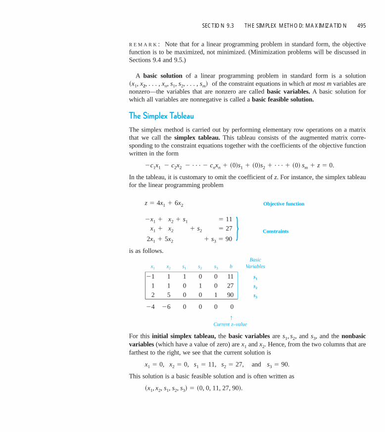
The Simplex TableauThe simplex method is carried out by performing elementary row operations on a matrixthat we call the simplex tableau.This tableau consists of the augmented matrix corre-sponding to the constraint equations together with the coefficients of the objective functionwritten in the form
In the tableau, it is customary to omit the coefficient of z. For instance, the simplex tableaufor the linear programming problem
Objective function
is as follows.Basic
x1 x2 s1 s2 s3 b Variables
1 1 0 0 11 s1
1 1 0 1 0 27 s2
2 5 0 0 1 90 s3
0 0 0 0
↑Current z–value
For this initial simplex tableau, the basic variables are and and the nonbasicvariables (which have a value of zero) are and . Hence, from the two columns that arefarthest to the right, we see that the current solution is
and
This solution is a basic feasible solution and is often written as
sx1, x2, s1, s2, s3d 5 s0, 0, 11, 27, 90d.
s3 5 90.x1 5 0, x2 5 0, s1 5 11, s2 5 27,
x2x1
s3,s1, s2,
2624
21
2x1 1 5x2 1 s1 1 s2 1 s3 5 90
2x1 1 5x2 1 s1 1 s2 1 s3 5 27
2x1 1 5x2 1 s1 1 s2 1 s3 5 11
z 5 4x1 1 6x2
2c1x1 2 c2x2 2 . . . 2 cnxn 1 s0ds1 1 s0ds2 1 . . . 1 s0d sm 1 z 5 0.
sx1, x2, . . . , xn, s1, s2, . . . , smd
SECTION 9.3 THE SIMPLEX METHOD: MAXIMIZATION 495
} Constraints

The entry in the lower–right corner of the simplex tableau is the current value of z. Notethat the bottom–row entries under and are the negatives of the coefficients of and
in the objective function
To perform an optimality check for a solution represented by a simplex tableau, we lookat the entries in the bottom row of the tableau. If any of these entries are negative (asabove), then the current solution is not optimal.
Pivoting
Once we have set up the initial simplex tableau for a linear programming problem, the sim-plex method consists of checking for optimality and then, if the current solution is not op-timal, improving the current solution. (An improved solution is one that has a larger z-valuethan the current solution.) To improve the current solution, we bring a new basic variableinto the solution––we call this variable the entering variable. This implies that one of thecurrent basic variables must leave, otherwise we would have too many variables for a basicsolution––we call this variable the departing variable. We choose the entering and departing variables as follows.1. The entering variable corresponds to the smallest (the most negative) entry in the
bottom row of the tableau.2. The departing variable corresponds to the smallest nonnegative ratio of , in the
column determined by the entering variable.3. The entry in the simplex tableau in the entering variable’s column and the departing
variable’s row is called the pivot.Finally, to form the improved solution, we apply Gauss-Jordan elimination to the columnthat contains the pivot, as illustrated in the following example. (This process is called pivoting.)
E X A M P L E 1 Pivoting to Find an Improved Solution
Use the simplex method to find an improved solution for the linear programming problemrepresented by the following tableau.
Basicx1 x2 s1 s2 s3 b Variables
1 1 0 0 11 s1
1 1 0 1 0 27 s2
2 5 0 0 1 90 s3
0 0 0 0
The objective function for this problem is z 5 4x1 1 6x2.
2624
21
biyaij
z 5 4x1 1 6x2.
x2
x1x2x1
496 CHAPTER 9 LINEAR PROGRAMMING
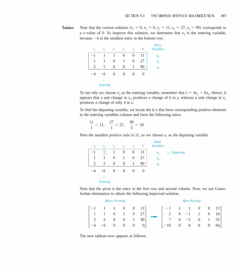
Solution Note that the current solution corresponds toa z–value of 0. To improve this solution, we determine that is the entering variable, because is the smallest entry in the bottom row.
Basicx1 x2 s1 s2 s3 b Variables
1 1 0 0 11 s1
1 1 0 1 0 27 s2
2 5 0 0 1 90 s3
0 0 0 0
↑Entering
To see whywe choose as the entering variable, remember that Hence, itappears that a unit change in produces a change of 6 in z, whereas a unit change in produces a change of only 4 in z.
To find the departing variable, we locate the ’s that have corresponding positive elementsin the entering variables column and form the following ratios.
Here the smallest positive ratio is 11, so we choose as the departing variable.
Basicx1 x2 s1 s2 s3 b Variables
1 1 0 0 11 s1 ← Departing
1 1 0 1 0 27 s2
2 5 0 0 1 90 s3
0 0 0 0
↑Entering
Note that the pivot is the entry in the first row and second column. Now, we use Gauss-Jordan elimination to obtain the following improved solution.
Before Pivoting After Pivoting
The new tableau now appears as follows.
321
2
7
210
1
0
0
0
1
21
25
6
0
1
0
0
0
0
1
0
11
16
35
6643
21
1
2
24
1
1
5
26
1
0
0
0
0
1
0
0
0
0
1
0
11
27
90
04
2624
21
s1
11
15 11,
27
15 27,
90
55 18
bi
x1x2
z 5 4x1 1 6x2.x2
2624
21
26x2
sx1 5 0, x2 5 0, s1 5 11, s2 5 27, s3 5 90d
SECTION 9.3 THE SIMPLEX METHOD: MAXIMIZATION 497

Basicx1 x2 s1 s2 s3 b Variables
1 1 0 0 11 x2
2 0 1 0 16 s2
7 0 0 1 35 s3
0 6 0 0 66
Note that has replaced in the basis column and the improved solution
has a z-value of
In Example 1 the improved solution is not yet optimal since the bottom row still has anegative entry. Thus, we can apply another iteration of the simplex method to further im-prove our solution as follows. We choose as the entering variable. Moreover, the small-est nonnegative ratio of and is 5, so is the departing variable. Gauss-Jordan elimination produces the following.
Thus, the new simplex tableau is as follows.
Basicx1 x2 s1 s2 s3 b Variables
0 1 0 16 x2
0 0 1 6 s2
1 0 0 5 x1
0 0 0 116
In this tableau, there is still a negative entry in the bottom row. Thus, we choose as theentering variable and as the departing variable, as shown in the following tableau.s2
s1
1072
87
172
57
227
37
17
27
30
0
1
0
1
0
0
0
2737
257
287
0
1
0
0
17
22717
107
16
6
5
1164
321
2
1
210
1
0
0
0
1
21
257
6
0
1
0
0
0
017
0
11
16
5
6643
21
2
7
210
1
0
0
0
1
21
25
6
0
1
0
0
0
0
1
0
11
16
35
664
s335y7 5 511ys21d, 16y2 5 8,x1
z 5 4x1 1 6x2 5 4s0d 1 6s11d 5 66.
sx1, x2, s1, s2, s3d 5 s0, 11, 0, 16, 35d
s1x2
210
25
21
21
498 CHAPTER 9 LINEAR PROGRAMMING

Basicx1 x2 s1 s2 s3 b Variables
0 1 0 16 x2
0 0 1 6 s2 ← Departing
1 0 0 5 x1
0 0 0 116
↑Entering
By performing one more iteration of the simplex method, we obtain the following tableau.(Try checking this.)
Basicx1 x2 s1 s2 s3 b Variables
0 1 0 12 x2
0 0 1 14 s1
1 0 0 15 x1
0 0 0 132 ← Maximum z-value
In this tableau, there are no negative elements in the bottom row. We have therefore deter-mined the optimal solution to be
with
R E M A R K : Ties may occur in choosing entering and/or departing variables. Should thishappen, any choice among the tied variables may be made.
Because the linear programming problem in Example 1 involved only two decision vari-ables, we could have used a graphical solution technique, as we did in Example 2, Section9.2. Notice in Figure 9.18 that each iteration in the simplex method corresponds to movingfrom a given vertex to an adjacent vertex with an improved z-value.
The Simplex Method
We summarize the steps involved in the simplex method as follows.
z 5 132z 5 116z 5 66z 5 0
s15, 12ds5, 16ds0, 11ds0, 0d
z 5 4x1 1 6x2 5 4s15d 1 6s12d 5 132.
sx1, x2, s1, s2, s3d 5 s15, 12, 14, 0, 0d
23
83
213
53
223
73
132
23
1072
87
172
57
227
37
17
27
SECTION 9.3 THE SIMPLEX METHOD: MAXIMIZATION 499
Figure 9.18
x1
x2
5
5
10
15
20
25
10 15 20 25 30
(0, 0)
(0, 11)
(5, 16)
(15, 12)
(27, 0)

Note that the basic feasible solution of an initial simplex tableau is
This solution is basic because at most m variables are nonzero (namely the slack variables).It is feasible because each variable is nonnegative.
In the next two examples, we illustrate the use of the simplex method to solve a problem involving three decision variables.
E X A M P L E 2 The Simplex Method with Three Decision Variables
Use the simplex method to find the maximum value of
Objective function
subject to the constraints
where and
Solution Using the basic feasible solution
the initial simplex tableau for this problem is as follows. (Try checking these computations,and note the “tie” that occurs when choosing the first entering variable.)
sx1, x2, x3, s1, s2, s3d 5 s0, 0, 0, 10, 20, 5d
x3 $ 0.x1 $ 0, x2 $ 0,
2x1 1 2x2 1 2x3 # 25
2x1 1 2x2 2 2x3 # 20
2x1 1 2x2 2 2x3 # 10
z 5 2x1 2 x2 1 2x3
sx1, x2, . . . , xn, s1, s2, . . . , sm d 5 s0, 0, . . . , 0, b1, b2, . . . , bm d.
500 CHAPTER 9 LINEAR PROGRAMMING
The Simplex Method(Standard Form)
To solve a linear programming problem in standard form, use the following steps.1. Convert each inequality in the set of constraints to an equation by adding slack
variables.2. Create the initial simplex tableau.3. Locate the most negative entry in the bottom row. The column for this entry is called
the entering column. (If ties occur, any of the tied entries can be used to determinethe entering column.)
4. Form the ratios of the entries in the “b-column” with their corresponding positive entries in the entering column. The departing row corresponds to the smallest non-negative ratio (If all entries in the entering column are 0 or negative, then thereis no maximum solution. For ties, choose either entry.) The entry in the departing rowand the entering column is called the pivot.
5. Use elementary row operations so that the pivot is 1, and all other entries in the entering column are 0. This process is called pivoting.
6. If all entries in the bottom row are zero or positive, this is the final tableau. If not, goback to Step 3.
7. If you obtain a final tableau, then the linear programming problem has a maximumsolution, which is given by the entry in the lower-right corner of the tableau.
biyaij .

Basicx1 x2 x3 s1 s2 s3 b Variables
2 1 0 1 0 0 10 s1
1 2 0 1 0 20 s2
0 1 2 0 0 1 5 s3 ← Departing
1 0 0 0 0
↑Entering
Basicx1 x2 x3 s1 s2 s3 b Variables
2 1 0 1 0 0 10 s1 ← Departing
1 3 0 0 1 1 25 s2
0 1 0 0 x3
2 0 0 0 1 5
↑Entering
Basicx1 x2 x3 s1 s2 s3 b Variables
1 0 0 0 5 x1
0 0 1 1 20 s2
0 1 0 0 x3
0 3 0 1 0 1 15
This implies that the optimal solution is
and the maximum value of z is 15.
Occasionally, the constraints in a linear programming problem will include an equation.In such cases, we still add a “slack variable” called an artificial variable to form the ini-tial simplex tableau. Technically, this new variable is not a slack variable (because there isno slack to be taken). Once you have determined an optimal solution in such a problem,you should check to see that any equations given in the original constraints are satisfied.Example 3 illustrates such a case.
E X A M P L E 3 The Simplex Method with Three Decision Variables
Use the simplex method to find the maximum value of
Objective functionz 5 3x1 1 2x2 1 x3
sx1, x2, x3, s1, s2, s3d 5 s5, 0, 52 , 0, 20, 0d
52
12
12
212
52
12
12
22
52
12
12
2222
22
SECTION 9.3 THE SIMPLEX METHOD: MAXIMIZATION 501
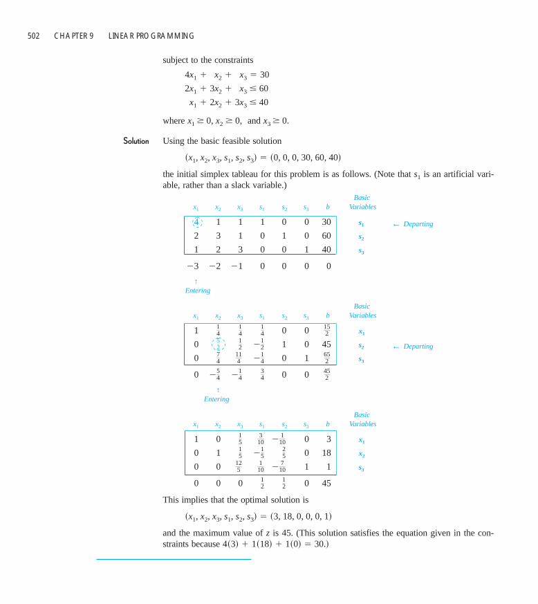
subject to the constraints
where and
Solution Using the basic feasible solution
the initial simplex tableau for this problem is as follows. (Note that is an artificial vari-able, rather than a slack variable.)
Basicx1 x2 x3 s1 s2 s3 b Variables
4 1 1 1 0 0 30 s1 ← Departing
2 3 1 0 1 0 60 s2
1 2 3 0 0 1 40 s3
0 0 0 0
↑Entering
Basicx1 x2 x3 s1 s2 s3 b Variables
1 0 0 x1
0 1 0 45 s2 ← Departing
0 0 1 s3
0 0 0
↑Entering
Basicx1 x2 x3 s1 s2 s3 b Variables
1 0 0 3 x1
0 1 0 18 x2
0 0 1 1 s3
0 0 0 0 45
This implies that the optimal solution is
and the maximum value of z is 45. (This solution satisfies the equation given in the con-straints because 4s3d 1 1s18d 1 1s0d 5 30.d
sx1, x2, x3, s1, s2, s3d 5 s3, 18, 0, 0, 0, 1d
12
12
2710
110
125
252
15
15
2110
310
15
452
342
142
54
6522
14
114
74
212
12
52
152
14
14
14
212223
s1
sx1, x2, x3, s1, s2, s3d 5 s0, 0, 0, 30, 60, 40d
x3 $ 0.x1 $ 0, x2 $ 0,
2x1 1 2x2 1 3x3 # 40
2x1 1 3x2 1 3x3 # 60
4x1 1 3x2 1 3x3 5 30
502 CHAPTER 9 LINEAR PROGRAMMING
Applications
E X A M P L E 4 A Business Application: Maximum Profit
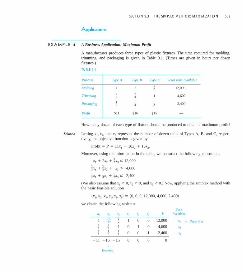
A manufacturer produces three types of plastic fixtures. The time required for molding,trimming, and packaging is given in Table 9.1. (Times are given in hours per dozen fixtures.)
TABLE 9.1
Process Type A Type B Type C Total time available
Molding 1 2 12,000
Trimming 1 4,600
Packaging 2,400
Profit $11 $16 $15 —
How many dozen of each type of fixture should be produced to obtain a maximum profit?
Solution Letting and represent the number of dozen units of Types A, B, and C, respec-tively, the objective function is given by
Profit
Moreover, using the information in the table, we construct the following constraints.
(We also assume that and ) Now, applying the simplex method withthe basic feasible solution
we obtain the following tableaus.Basic
x1 x2 x3 s1 s2 s3 b Variables
1 2 1 0 0 12,000 s1 ← Departing
1 0 1 0 4,600 s2
0 0 1 2,400 s3
0 0 0 0
↑Entering
215216211
12
13
12
23
23
32
sx1, x2, x3, s1, s2, s3d 5 s0, 0, 0, 12,000, 4,600, 2,400d
x3 $ 0.x1 $ 0, x2 $ 0,
12x1 1
13x2 1
12x3 # 12,400
23x1 1
23x2 1
32x3 # 14,600
23x1 1 2x2 1
32x3 # 12,000
5 P 5 11x1 1 16x2 1 15x3.
x3x1, x2,
12
13
12
23
23
32
SECTION 9.3 THE SIMPLEX METHOD: MAXIMIZATION 503

Basicx1 x2 x3 s1 s2 s3 b Variables
1 0 0 6,000 x2
0 1 0 600 s2
0 0 1 400 s3 ← Departing
0 −3 8 0 0 96,000
↑Entering
Basicx1 x2 x3 s1 s2 s3 b Variables
0 1 0 5,400 x2
0 0 1 200 s2 ← Departing
1 0 0 3 1,200 x1
0 0 0 9 99,600
↑Entering
Basicx1 x2 x3 s1 s2 s3 b Variables
0 1 0 1 0 5,100 x2
0 0 1 4 800 x3
1 0 0 0 6 600 x1
0 0 0 6 3 6 100,200
From this final simplex tableau, we see that the maximum profit is $100,200, and this isobtained by the following production levels.
Type A: 600 dozen units
Type B: 5,100 dozen units
Type C: 800 dozen units
R E M A R K : In Example 4, note that the second simplex tableau contains a “tie” for theminimum entry in the bottom row. (Both the first and third entries in the bottom row are
) Although we chose the first column to represent the departing variable, we could havechosen the third column. Try reworking the problem with this choice to see that you obtainthe same solution.
E X A M P L E 5 A Business Application: Media Selection
The advertising alternatives for a company include television, radio, and newspaper advertisements. The costs and estimates for audience coverage are given in Table 9.2
23.
23
24223
232
1322
34
212
34
21216
14
232
34
38
23
216
14
13
213
12
13
12
34
12
504 CHAPTER 9 LINEAR PROGRAMMING

TABLE 9.2
Television Newspaper Radio
Cost per advertisement $ 2,000 $ 600 $ 300
Audience per advertisement 100,000 40,000 18,000
The local newspaper limits the number of weekly advertisements from a single company toten. Moreover, in order to balance the advertising among the three types of media, no morethan half of the total number of advertisements should occur on the radio, and at least 10%should occur on television. The weekly advertising budget is $18,200. How many adver-tisements should be run in each of the three types of media to maximize the total audience?
Solution To begin, we let and represent the number of advertisements in television, news-paper, and radio, respectively. The objective function (to be maximized) is therefore
Objective function
where and The constraints for this problem are as follows.
A more manageable form of this system of constraints is as follows.
Thus, the initial simplex tableau is as follows.
Basicx1 x2 x3 s1 s2 s3 s4 b Variables
20 6 3 1 0 0 0 182 s1 ← Departing
0 1 0 0 1 0 0 10 s2
1 0 0 1 0 0 s3
1 1 0 0 0 1 0 s4
0 0 0 0 0
↑Entering
218,000240,0002100,000
29
2121
29x1 1 6x2 1 3x3 # 180
2x1 2 6x2 1 3x3 # 180
20x1 1 6x2 1 3x3 # 110
20x1 1 6x2 1 3x3 # 182
2000x1 1 600x2 1 300x3 $ 0.1sx1 1 x2 1 x3d
2000x1 1 600x2 1 300x3# 0.5sx1 1 x2 1 x3d
2000x1 1 600x2 1 300x3 # 10
2000x1 1 600x2 1 300x3 # 18,200
x3 $ 0.x1 $ 0, x2 $ 0,
z 5 100,000x1 1 40,000x2 1 18,000x3
x3x1, x2,
SECTION 9.3 THE SIMPLEX METHOD: MAXIMIZATION 505
} Constraints

Now, to this initial tableau, we apply the simplex method as follows.Basic
x1 x2 x3 s1 s2 s3 s4 b Variables
1 0 0 0 x1
0 1 0 0 1 0 0 10 s2 ← Departing
0 0 1 0 s3
0 0 0 1 s4
0 5,000 0 0 0 910,000↑
Entering
Basicx1 x2 x3 s1 s2 s3 s4 b Variables
1 0 0 0 x1
0 1 0 0 1 0 0 10 x2
0 0 1 0 s3 ← Departing
0 0 0 1 s4
0 0 5,000 10,000 0 0 1,010,000
↑Entering
Basicx1 x2 x3 s1 s2 s3 s4 b Variables
1 0 0 0 4 x1
0 1 0 0 1 0 0 10 x2
0 0 1 0 14 x3
0 0 0 1 12 s4
0 0 0 0 1,052,000
From this tableau, we see that the maximum weekly audience for an advertising budget of$18,200 is
Maximum weekly audience
and this occurs when and We sum up the results here.
Number ofMedia Advertisements Cost Audience
Television 4 $ 8,000 400,000
Newspaper 10 $ 6,000 400,000
Radio 14 $ 4,200 252,000
Total 28 $18,200 1,052,000
x3 5 14.x1 5 4, x2 5 10,
z 5 1,052,000
60,00023
272,00023
118,00023
247232
11823
823
2023
1423
123
23232
923
123
23,000
449102
3710
920
4720
16110
710
120
2320
61102
310
120
320
23,000210,000
81910
920
4720
3710
9110
120
23202
710
9110
120
320
310
506 CHAPTER 9 LINEAR PROGRAMMING

SECTION 9.3 EXERCISES 507
In Exercises 1– 4, write the simplex tableau for the given linear pro-gramming problem. You do not need to solve the problem. (In eachcase the objective function is to be maximized.)
1. Objective function: 2. Objective function:
Constraints: Constraints:
3. Objective function: 4. Objective function:
Constraints: Constraints:
In Exercises 5–8, explain why the linear programming problem isnot in standard form as given.5. (Minimize) 6. (Maximize)
Objective function: Objective function:
Constraints: Constraints:
7. (Maximize) 8. (Maximize)Objective function: Objective function:
Constraints: Constraints:
In Exercises 9–20, use the simplex method to solve the givenlinear programming problem. (In each case the objective functionis to be maximized.)
9. Objective function: 10. Objective function:
Constraints: Constraints:
x1, x2 $ 10x1, x2 $ 103x1 1 2x2 # 12x1 1 4x2 # 123x1 1 2x2 # 16x1 1 4x2 # 18
z 5 x1 1 x2z 5 x1 1 2x2
x1, x2, x3 $ 0x1, x2 $ 02x1 1 x2 1 3x3 # 0
2x1 1 x2 $ 62x1 1 x2 2 2x3 $ 1x1 1 x2 $ 42x1 1 x2 1 3x3 # 5
z 5 x1 1 x2z 5 x1 1 x2
x1, x2 $ 202x1 2 2x2 # 21 x1, x2 $ 02x1 1 2x2 # 26x1 1 2x2 # 4
z 5 x1 1 x2z 5 x1 1 x2
x1, x2 $ 20x1, x2, x3 $ 10
2x1 1 3x2 # 20x1 1 2x2 1 x3 # 18
2x1 2 3x2 # 26x1 1 2x2 1 x3 # 12
z 5 6x1 2 9x2z 5 2x1 1 3x2 1 4x3
x1, x2 $ 02x1, x2 $ 0x1 2 x2 # 12x1 1 x2 # 5x1 1 x2 # 42x1 1 x2 # 8
z 5 x1 1 3x2z 5 x1 1 2x2
SECTION 9.3 ❑ EXERCISES
11. Objective function: 12. Objective function:
Constraints: Constraints:
13. Objective function: 14. Objective function:
Constraints: Constraints:
15. Objective function: 16. Objective function:
Constraints: Constraints:
17. Objective function: 18. Objective function:
Constraints: Constraints:
19. Objective function:
Constraints:
20. Objective function:
Constraints:
x1, x2, x3, x4 $ 702x1 1 3x2 1 2x3 1 6x4 # 722x1 1 3x2 1 2x3 1 5x4 # 502x1 1 3x2 1 3x3 1 4x4 # 60
z 5 x1 1 2x2 1 x3 2 x4
x1, x2, x3, x4 $ 40x1 1 3x2 1 7x3 1 x4 # 42x1 1 2x2 1 3x3 1 x4 # 24
z 5 x1 1 2x2 2 x4
x1, x2, x3 $ 50x1, x2, x3 $ 302x1 1 x2 1 6x3 # 542x1 1 2x2 1 3x3 # 322x1 1 x2 1 3x3 # 752x1 1 2x2 1 3x3 # 252x1 1 x2 1 3x3 # 592x1 1 2x2 2 3x3 # 40
z 5 2x1 1 x2 1 3x3z 5 x1 2 x2 1 x3
x1, x2 $ 40x1, x2, x3, x4 $ 03x1 1 4x2 # 482x1 1 4x2 1 5x3 1 2x4 # 83x1 1 2x2 # 282x1 1 6x2 1 4x3 1 5x4 # 33x1 1 2x2 # 608x1 1 3x2 1 4x3 1 5x4 # 7
z 5 x1z 5 3x1 1 4x2 1 x3 1 7x4
x1, x2 $ 10x1, x2 $ 402x1 2 3x2 # 123x1 1 7x2 # 422x1 1 3x2 # 153x1 1 7x2 # 10
z 5 x1 1 2x2z 5 4x1 1 5x2
x1, x2, x3 $ 40x1, x2, x3 $ 06x1 2 3x2 1 3x3 # 42
2x1 1 2x3 # 52x1 1 3x2 2 3x3 # 422x1 1 2x2 # 82x1 2 4x2 1 3x3 # 42
z 5 x1 2 x2 1 2x3z 5 5x1 1 2x2 1 8x3

508 CHAPTER 9 LINEAR PROGRAMMING
21. A merchant plans to sell two models of home computers atcosts of $250 and $400, respectively. The $250 model yields aprofit of $45 and the $400 model yields a profit of $50. Themerchant estimates that the total monthly demand will notexceed 250 units. Find the number of units of each model thatshould be stocked in order to maximize profit. Assume thatthe merchant does not want to invest more than $70,000 incomputer inventory. (See Exercise 21 in Section 9.2.)
22. A fruit grower has 150 acres of land available to raise twocrops, A and B. It takes one day to trim an acre of crop A andtwo days to trim an acre of crop B, and there are 240 days peryear available for trimming. It takes 0.3 day to pick an acre ofcrop A and 0.1 day to pick an acre of crop B, and there are 30days per year available for picking. Find the number of acresof each fruit that should be planted to maximize profit, as-suming that the profit is $140 per acre for crop A and $235per acre for B. (See Exercise 22 in Section 9.2.)
23. A grower has 50 acres of land for which she plans to raisethree crops. It costs $200 to produce an acre of carrots andthe profit is $60 per acre. It costs $80 to produce an acre ofcelery and the profit is $20 per acre. Finally, it costs $140 toproduce an acre of lettuce and the profit is $30 per acre. Usethe simplex method to find the number of acres of each cropshe should plant in order to maximize her profit. Assume thather cost cannot exceed $10,000.
24. A fruit juice company makes two special drinks by blendingapple and pineapple juices. The first drink uses 30% applejuice and 70% pineapple, while the second drink uses 60%apple and 40% pineapple. There are 1000 liters of apple and1500 liters of pineapple juice available. If the profit for thefirst drink is $0.60 per liter and that for the second drink is$0.50, use the simplex method to find the number of liters ofeach drink that should be produced in order to maximize theprofit.
25. A manufacturer produces three models of bicycles. The time(in hours) required for assembling, painting, and packagingeach model is as follows.
Model A Model B Model C
Assembling 2 2.5 3
Painting 1.5 2 1
Packaging 1 0.75 1.25
The total time available for assembling, painting, and packag-ing is 4006 hours, 2495 hours and 1500 hours, respectively.The profit per unit for each model is $45 (Model A), $50(Model B), and $55 (Model C). How many of each typeshould be produced to obtain a maximum profit?
26. Suppose in Exercise 25 the total time available for assem-bling, painting, and packaging is 4000 hours, 2500 hours, and1500 hours, respectively, and that the profit per unit is $48(Model A), $50 (Model B), and $52 (Model C). How manyof each type should be produced to obtain a maximum profit?
27. A company has budgeted a maximum of $600,000 for adver-tising a certain product nationally. Each minute of televisiontime costs $60,000 and each one-page newspaper ad costs$15,000. Each television ad is expected to be viewed by 15million viewers, and each newspaper ad is expected to beseen by 3 million readers. The company’s market research department advises the company to use at most 90% of theadvertising budget on television ads. How should the advertising budget be allocated to maximize the total audi-ence?
28. Rework Exercise 27 assuming that each one-page newspaperad costs $30,000.
29. An investor has up to $250,000 to invest in three types of in-vestments. Type A pays 8% annually and has a risk factor of0. Type B pays 10% annually and has a risk factor of 0.06.Type C pays 14% annually and has a risk factor of 0.10. Tohave a well-balanced portfolio, the investor imposes the fol-lowing conditions. The average risk factor should be nogreater than 0.05. Moreover, at least one-fourth of the totalportfolio is to be allocated to Type A investments and at leastone-fourth of the portfolio is to be allocated to Type B invest-ments. How much should be allocated to each type of invest-ment to obtain a maximum return?
30. An investor has up to $450,000 to invest in three types of investments. Type A pays 6% annually and has a risk factorof 0. Type B pays 10% annually and has a risk factor of 0.06.Type C pays 12% annually and has a risk factor of 0.08. Tohave a well-balanced portfolio, the investor imposes the following conditions. The average risk factor should be nogreater than 0.05. Moreover, at least one-half of the total portfolio is to be allocated to Type A investments and at leastone-fourth of the portfolio is to be allocated to Type B invest-ments. How much should be allocated to each type of investment to obtain a maximum return?
31. An accounting firm has 900 hours of staff time and 100 hoursof reviewing time available each week. The firm charges$2000 for an audit and $300 for a tax return. Each audit requires 100 hours of staff time and 10 hours of review time,and each tax return requires 12.5 hours of staff time and 2.5hours of review time. What number of audits and tax returnswill bring in a maximum revenue?

SECTION 9.4 THE SIMPLEX METHOD: MINIMIZATION 509
32. The accounting firm in Exercise 31 raises its charge for anaudit to $2500. What number of audits and tax returns willbring in a maximum revenue?
In the simplex method, it may happen that in selecting the departingvariable all the calculated ratios are negative. This indicates an un-bounded solution. Demonstrate this in Exercises 33 and 34.
33. (Maximize) 34. (Maximize)Objective function: Objective function:
Constraints: Constraints:
If the simplex method terminates and one or more variables not inthe final basishave bottom-row entries of zero, bringing these variables into the basis will determine other optimal solutions.Demonstrate this in Exercises 35 and 36.
x1, x2 $
50x1, x2 $ 022x1 1 x2 # 502x1 1 2x2 # 4 2x1 1 x2 # 202x1 2 3x2 # 1
z 5 x1 1 3x2z 5 x1 1 2x2
35. (Maximize) 36. (Maximize)Objective function: Objective function:
Constraints: Constraints:
37. Use a computer to maximize the objective function
subject to the constraints
where
38. Use a computer to maximize the objective function
subject to the same set of constraints given in Exercise 37.
z 5 1.2x1 1 x2 1 x3 1 x4
x1, x2, x3, x4 $ 0.
0.5x1 1 0.7x2 1 01.2x3 1 0.4x4 # 801.2x1 1 0.7x2 1 0.83x3 1 1.2x4 # 961.2x1 1 0.7x2 1 0.83x3 1 0.5x4 # 65
z 5 2x1 1 7x2 1 6x3 1 4x4
x1, x2 $ 30x1, x2 $ 102x1 1 3x2 # 355x1 1 2x2 # 102x1 1 3x2 # 203x1 1 5x2 # 15
z 5 x1 112 x2z 5 2.5x1 1 x2
9.4 THE SIMPLEX METHOD: MINIMIZATION
In Section 9.3, we applied the simplex method only to linear programming problems instandard form where the objective function was to be maximized. In this section, we extendthis procedure to linear programming problems in which the objective function is to be min-imized.
A minimization problem is in standard form if the objective function is to be minimized, subject to the constraints
where The basic procedure used to solve such a problem is to convert itto a maximization problemin standard form, and then apply the simplex method as dis-cussed in Section 9.3.
In Example 5 in Section 9.2, we used geometric methods to solve the following minimization problem.
xi $ 0 and bi $ 0.
am1x1 1 am2x2 1 . . . 1 amnxn $ bm
...
a21x1 1 a22x2 1 . . . 1 a2nxn $ b2
a11x1 1 a12x2 1 . . . 1 a1nxn $ b1
1 . . . 1 cnxn
c1x1 1 c2x2w 5
C
C