79

Linear Programming UNIT 4 LINEAR PROGRAMMING

Structure

4.0 Introduction

4.1 Objectives

4.2 Linear Programming

4.3 Techniques of Solving Linear Programming Problem

4.4 Cost Minimisation

4.5 Answers to Check Your Progress

4.6 Summary

4.0 INTRODUCTION

We first make the idea clear through an illustration.

Suppose a furniture company makes chairs and tables only. Each chair gives

a profit of ` 20 whereas each table gives a profit of `30. Both products are

processed by three machines Ml, M2 and M3. Each chair requires 3 hrs 5 hrs

and 2 hrs on Ml, M2 and M3. respectively, whereas the corresponding figures

for each table are 3, 2, 6. The machine M l can work for 36 hrs per week,

whereas M2 and M3 can work for 50 hrs and 60 hrs, respectively. How many

chairs and tables should be manufactured per week to maximise the profit?

We begin by assuming that x chairs and y tables, be manufactured per week.

The profit of the company will be ` (20x + 30y) per week. Since the objective

of the company is to maximise its profit, we have to find out the maximum

possible value of P = 20x + 30y. We call this as the objective function.

To manufacture x chairs and y tables, the company will require (3x + 3y) hrs

on machine M1 . But the total time available on machine M1 is 36 hrs.

Therefore, we have a constraint 3x + 3y ≤ 36.

Similarly, we have the constraint 5x + 2y ≤ 50 for the machine M2 and the

constraint 2x + 6y ≤ 60 for the machine M3.

Also since it is not possible for the company to produce negative number of

chairs and tables, we must have x ≥ 0 and y ≥ 0. The above problem can now be

written in the following format :

80

Vectors and Three

Dimensional Geometry

Maximise

P = 20x + 30y

subject to

3x + 3y ≤ 36

5x + 2 y ≤ 50

2 x + 6y ≤ 60

and x ≥ 0, y ≥ 0

We now plot the region bounded by constraints in Fig. 1 The shaded region is

called the feasible region or the solution space as the coordinators of any point

lying in this region always satisfy the constraints. Students are encouraged to

verify this by taking points (2,2),(2,4) (4,2) which lies in the feasible region.

0 10 12 30

5x + 2y =

50

2x + 6y = 60

3x + 3y = 36

2525

12

10

(3,9)

Figure 1

We redraw the feasible region without shading to clarify another concept (see

Figure 2).

For any particular value of P, we can draw in the objective function as a straight

line with slope 2

3 This is because P = 20x + 30 y is a straight line, which

can be written as

2 =

3 30

Py x

81

Linear Programming

10 Figure 2

and this generates a family of parallel lines with slope but with different

intercepts on the axes. On any particular line, the different combinations of x

and y (chairs and tables) all yield the same profit (P).

higher y-intercepts yield higher profits.

The problem is therefore to maximise the y-intercept, while at the same time

remaining within constraints (or, feasible region). The part of the profit line

which fall within the feasible region have been heavily drawn. Profit lines drawn

farthest away from the origin (0, 0) yield the highest profits. Therefore, the

highest profit yielded within the feasible region is at point B(3, 9). Therefore,

the maximum profit is given by ` (20× 3 + 30× 9) = ` 330.

We are now ready for the definition of linear programming – the technique of

solving the problem such as above.

What is Linear Programming

Linear because the equations and relationships introduced are linear. Note that

all the constraints and the objective functions are linear. Programming is used in

the sense of method, rather than in the computing sense.

B(3,9)

A(0,10)

‘Equal Profit’ lines

Direction of

Increasing Profit

10

0(0,0)

82

Vectors and Three

Dimensional Geometry

In fact, linear programming is a technique for specifying how to use limited

resources or capacities of a business to obtain a particular objective, such as

least cost, highest margin or least time, when those resources have alternative

uses.

4.1 OBJECTIVES

After studying this unit, you should be able to:

define the terms-objective function, constraints, feasible region,

feasible solution, optimal solution and linear programming;

draw feasible region and use it to obtain optimal solution;

tell when there are more than one optimal solutions; and

know when the problem has no optimal solution.

4.2 LINEAR PROGRAMMING

We begin by listing some definitions.

Definitions

* In this unit we shall work with just two variables.

Objective Functions: If a1, a2, . . . , an are constants and x1 x2, ..., xn are

variables, then the linear function Z = a1x1 + a2x2 +...+ anxn which is to be

maximised or minimised is called objective function*.

Constraints: These are the restrictions to be satisfied by the variables x1,

x2 ..., xn. These are usually expressed as inequations and equations.

Non-negative Restrictions: The values of the variables x1 x2, ..., xn

involved in the linear programming problem (LPP) are greater than or

equal to zero (This is so because most of the variable represent some

economic or physical variable.)

Feasible Region: The common region determined by all the constraints of

an LPP is called the feasible region of the LPP.

Feasible Solution: Every point that lies in the feasible region is called a

feasible solution. Note that each point in the feasible region satisfies all the

constraints for the LPP.

Optimal Solution: A feasible solution that maximises or minimizes the

objective function is called an optimal solution of the LPP.

83

Linear Programming

A

Definition

The student may observe that a feasible region for a linear programming is a

convex region.

One of the properties of the convex region is that maximum and minimum values

of a function defined on convex regions occur at the corner points only. Since

all feasible regions are convex regions, maximum and minimum values of

optimal functions occur at the corner points of the feasible region.

The region of Figure 3 is convex but that of Figure 4 is not convex.

y y

o x o x

Figure 3 : Convex Region Figure 4 : Not Convex

4.3 TECHNIQUES OF SOLVING LINEAR PROGRAMMING

PROBLEM

There are two techniques of solving an L.P.P. (Linear Programming Problem)

by graphical method. These are

(i) Corner point method, and

(ii) Iso profit or Iso-cost method.

The following procedure lists the coner point method.

* The method explained in Example 1 is the iso-profit method. You are advised to use corner

method unless you are specifically asked to do the problem by the iso-profit or iso-cost

method.

Convex Region

A region R in the coordinate plane is said to be convex if whenever we take two

points A and B in the region R, the segment joining A and B lies completely in

R.

B

B

B

A

Corner Point Method*

Step 1 Plot the feasible region.

Step 2 Find the coordinates of the cornor points of the feasible region.

Step 3 Calculate the value of the objective function at each of the corner points

of the feasible region.

Step 4 Pick up the maximum (or minimum) value of the objective function

from amongst the points in step 3.

A

84

Vectors and Three

Dimensional Geometry

Example 1 Find the maximum value of 5x + 2y subject to the constraints

–2x – 3y ≤ –6

x – 2y ≤ 2

6x + 4y ≤ 24

–3x +2y ≤ 3

x ≥ 0, y ≥ 0.

Solution

Let us denote 5x + 2y by P.

Note that –2x –3y ≤ –6 can be written as 2x + 3 y ≥ 6.

We can write the given LPP in the following format :

Maximise

P = 5x + 2y

subject to

2x + 3y ≥ 6 (I)

x – 2y ≤ 2 (II)

6x + 4y ≤ 24 (III)

–3x +2y ≤ 3 (IV)

and x ≥ 0, y ≥ 0

We plot the feasible region bounded by the given constraints in Figure 5

The lines I and II intersect in A (18/7, 2/7)

The lines II and III intersect in B (7/2, 3/4)

The lines III and IV intersect in C (3/2, 15/4)

The lines IV and I intersect in D (3/13, 24/13)

Let us evaluate P at A, B, C and D

P(A) = 5 (18/7) + (2/7) = 94/7 P(B) = 5 (7/2) + 2(3/4) =19

P(C) = 5 (3/2) + 2(15/4) = 15 P(D) = 5 (3/13) + 2(24/13)= 63/13

Thus, maximum value of P is 19 and its occurs at x = 7/2, y =3/4.

85

Linear Programming

-

6x + 4 y =

24

2x +3 y = 6

x -2 y =

2

-3x +2y

= 3

II

III

IV

II

0 1 2 3 4 5 6

-1

B(7/2

,3/4)

C (3/

2,15

/4)

Figure 5

Example 2 Find the maximum value of 2x + y subject to the constraints

x + 3y ≥ 6

x – 3y ≤ 3

3x + 4y ≤ 24

–3x + 2y ≤ 6

5x + y ≥ 5

x, y ≥ 0

Solution

We write the given question in the following format :

Maximise

P = 2x + y

subject to

x + 3y ≥ 6 (I)

x – 3y ≤ 3 (II)

3x + 4y ≤ 24 (III)

–3x + 2y ≤ 6 (IV)

5x + y ≥ 5 (V)

and x≥ 0, y ≥ 0 (VI)

A

D

86

Vectors and Three

Dimensional Geometry

The feasible region is sketched in Figure 6

The lines I and II intersect in A(9/2, 1/2)

The lines II and III intersect in B(84/13, 15/13)

The lines III and IV intersect in C(4/3, 5)

The lines IV and V intersect in D(4/13, 45/13)

The lines V and I intersect in E(9/14, 25/14).

Let us evaluate P at the points A, B, C, D and E as follows:

P(A) = 2(9/2) + 1/2 = 19/2

P(B) = 2(84/13) + 15/13 = 183/13

P(C) = 2(4/3) + 5 = 23/3

P(D) = 2(4/13) + 45/13 = 53/13

P(E) = 2(9/14) + 25/14 = 43/14

The maximum value of P is 183/13 which occurs at x = 84/13 and y = 15/13.

Example 3: An aeroplane can carry a maximum of 200 passengers. A profit of

` 400 is made on each first class ticket and a profit of ` 300 is made on

each economy class ticket. The airline reserves at least 20 seats for first class.

However, at least 4 times as many passengers prefer to travel by economy

class than by first class. Determine how many of each type of tickets must be

sold in order to maximise the profit for the airline? What is the maximum profit?

C(4/3,5)

A(9/2,1/2) -2 -1 0 1 2 3 4 5 8

5

4

3

2

1

Y

6

V

III

V

II

IV

I

Figure 6

B

E

87

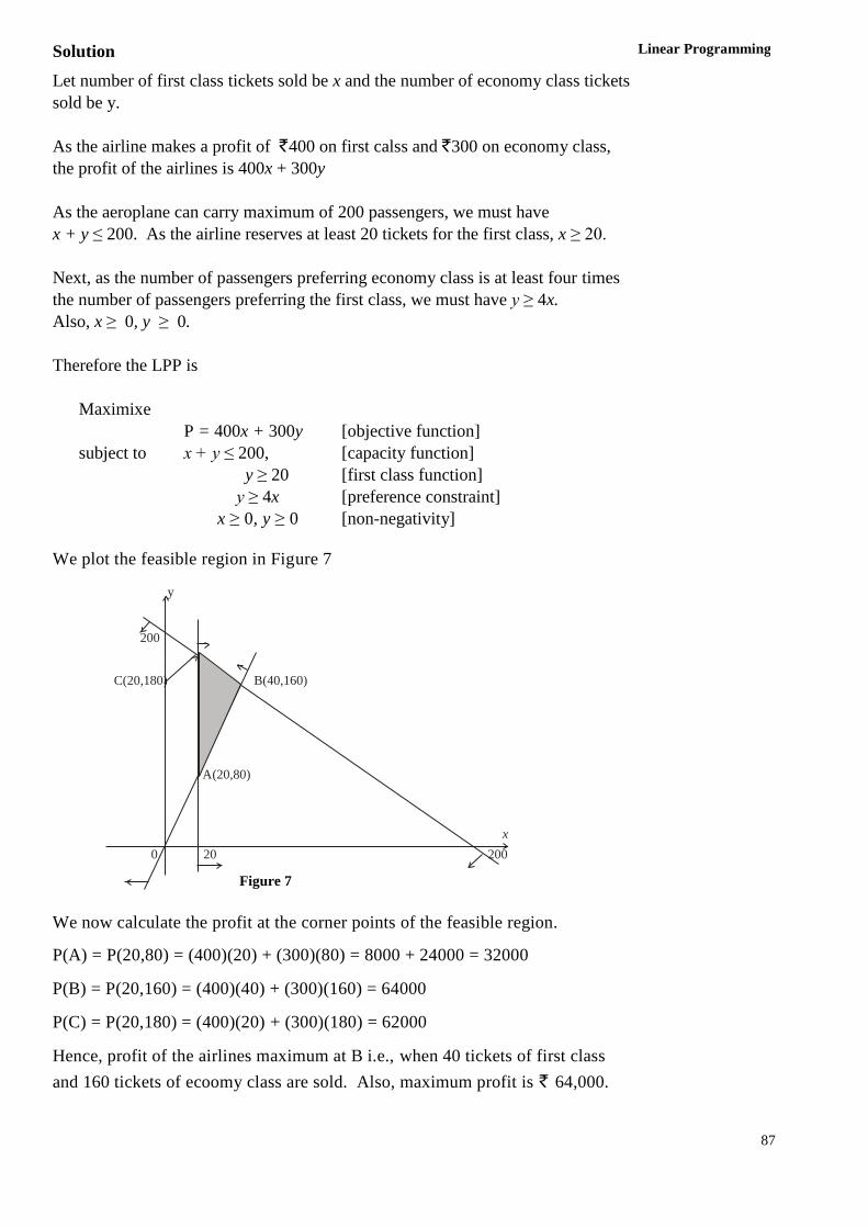
Linear Programming Solution

Let number of first class tickets sold be x and the number of economy class tickets

sold be y.

As the airline makes a profit of `400 on first calss and `300 on economy class,

the profit of the airlines is 400x + 300y

As the aeroplane can carry maximum of 200 passengers, we must have

x + y ≤ 200. As the airline reserves at least 20 tickets for the first class, x ≥ 20.

Next, as the number of passengers preferring economy class is at least four times

the number of passengers preferring the first class, we must have y ≥ 4x.

Also, x ≥ 0, y ≥ 0.

Therefore the LPP is

Maximixe

P = 400x + 300y [objective function]

subject to x + y ≤ 200, [capacity function]

y ≥ 20 [first class function]

y ≥ 4x [preference constraint]

x ≥ 0, y ≥ 0 [non-negativity]

We plot the feasible region in Figure 7

We now calculate the profit at the corner points of the feasible region.

P(A) = P(20,80) = (400)(20) + (300)(80) = 8000 + 24000 = 32000

P(B) = P(20,160) = (400)(40) + (300)(160) = 64000

P(C) = P(20,180) = (400)(20) + (300)(180) = 62000

Hence, profit of the airlines maximum at B i.e., when 40 tickets of first class

and 160 tickets of ecoomy class are sold. Also, maximum profit is ` 64,000.

200

C(20,180)

A(20,80)

B(40,160)

0 20 200

x

y

Figure 7Figure 7

88

Vectors and Three

Dimensional Geometry

Example 4: Suriti wants to invest at most ` 12000 in Savings Certificate and

National Savings Bonds. She has to invest at least ` 2000 in Savings

Certificate and at least ` 4000 in National Savings Bonds. If the rate of interest

in Saving Certificate is 8% per annum and the rate of interest on National

Saving Bond is 10% per annum, how much money should she invest to earn

maximum yearly income ? Find also the maximum yearly income ?

Solution

Suppose Suriti invests ` x in saving certificate and ` y in National Savings

Bonds.

As she has just ` 12000 to invest, we must have x + y ≤ 12000.

Also, as she has to invest at least ` 2000 in savings certificate x ≥ 2000.

Next, as she must invest at least Rs. 4000 in National Savings Certificate

y ≥ 4000. Yearly income from saving certificate = ` = 0.08x and from

National Savings Bonds = ` = Rs. 0.1y

Her total income is ` P where

P = 0.08x + 0.1y

Thus, the linear programming problem is

Maximise

subject to

x + y ≤ 12000 [Total Money Constraint]

x ≥ 2000 [Savings Certificate Constraint]

y ≥ 4000 [National Savings Bonds Constraint]

x ≥ 0, y ≥ 0 [ Non-negativity Constraint]

However, note that the constraints x ≥ 0, y ≥0, are redundant in view of

x ≥ 2000 and y ≥ 4000.

We draw the feasible region in Figure 8

89

Linear Programming

12000C(2000,10000)

Y = 4000

4000 A(2000, 4000) B(8000, 4000)

X = 2000

120002000

x + y = 12000

Y

x

0

Figure 8

We now calculate the profit at the corner points of the feasible region.

We have

P(A) = P(2000,4000) = (0.08) (2000) + (0.1)(4000)

= 160 +400 = 560

P(B) = P(8000,4000) = (0.08) (2000) + (0.1)(4000)

= 640 +400 = 1040

P(C) = P(2000,10000) = (0.08) (2000) + (0.1)(10000)

= 160 +1000 =1160.

Thus, she must invest ` 2000 in Savings certificate and ` 10000 in National

Savings Bonds in order to earn maximum income.

Example 5 If a young man rides his motor cycle at 25 km per hour, he has to

spend ` 2 per km on petrol; if he rides it at a faster speed of 40 km per hour,

the petrol cost increases to ` 5 per km. He wishes to spend at most ` 100 on

petrol and wishes to find what is maximum distance he can travel within one

hour. Express this as a linear programming problem and then solve it.

Solution

Let x km be the distance travlled at the rate of 25 km/h and y km be the

distance travelled at the rate of 40 km/h. Then the total distance covered by the

young man is D = (x + y) km.

The money spent in travelling x km (at the rate of 25 km/h) is 2x and the money

spent in travelling y km (at the rate of 40 km/h) is 5y. Thus, total money spent

during the journey is ` (2x +5y). Since the young man wishes to spend at most

Rs. 100 on the journey, we must have 2x + 5y ≤ 100.

90

Vectors and Three

Dimensional Geometry

Also, note that x ≥ 0, y ≥ 0.

The mathematical formulation of the linear programming problem is

Maximise

D = x + y

subject to

2x + 5y ≤ 100

and x ≥ 0, y ≥ 0.

The feasible region is sketched in Figure 9. Y

0 10 20 30 40 50

40

30

20

10

A(25,0)

C(0

,20)

x

Figure 9 The corner points of feasible region are O(0,0), A(25,0),

Let us evaluate D at these points

D(O) = 0 + 0 = 0

D(A) = 25 + 0 = 25

D(C) = 0 + 20 = 20

Thus, the maximum values of D is 30 which occurs at x = 50/3, y = 40/3

B 50

3,40

3

A(25,0)

Figure 9

x

91

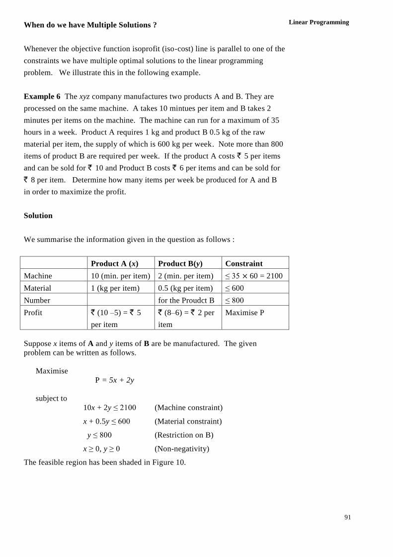
Linear Programming When do we have Multiple Solutions ?

Whenever the objective function isoprofit (iso-cost) line is parallel to one of the

constraints we have multiple optimal solutions to the linear programming

problem. We illustrate this in the following example.

Example 6 The xyz company manufactures two products A and B. They are

processed on the same machine. A takes 10 mintues per item and B takes 2

minutes per items on the machine. The machine can run for a maximum of 35

hours in a week. Product A requires 1 kg and product B 0.5 kg of the raw

material per item, the supply of which is 600 kg per week. Note more than 800

items of product B are required per week. If the product A costs ` 5 per items

and can be sold for ` 10 and Product B costs ` 6 per items and can be sold for

` 8 per item. Determine how many items per week be produced for A and B

in order to maximize the profit.

Solution

We summarise the information given in the question as follows :

Product A (x) Product B(y) Constraint

Machine 10 (min. per item) 2 (min. per item) ≤ 35 60 = 2100

Material 1 (kg per item) 0.5 (kg per item) ≤ 600

Number for the Proudct B ≤ 800

Profit ` (10 –5) = ` 5

per item

` (8–6) = ` 2 per

item

Maximise P

Suppose x items of A and y items of B are be manufactured. The given

problem can be written as follows.

Maximise

P = 5x + 2y

subject to

10x + 2y ≤ 2100 (Machine constraint)

x + 0.5y ≤ 600 (Material constraint)

y ≤ 800 (Restriction on B)

x ≥ 0, y ≥ 0 (Non-negativity)

The feasible region has been shaded in Figure 10.

92

Vectors and Three

Dimensional Geometry

0(0,0) 100 200 300 400 500 600x

y

1200

1000

800

600

400

200

Y = 800

A(0,800)

C(210,0)

B(50,800)

x + 0.5y = 600

10x +

2y =

600

Figure 10

We now calculate the value of P at the corner points of the feasible region

P(A) = P(0,800) = 1600

P(B) = P(50,800) = 1850

P(C) = P(210,0) = 1050

P(O) = P(0,0) = 0

Maximum profit is ` 1850 for x = 50 and y = 800

Redundant Constraints

In the above example, the constraitn x + 0.5, y ≤ 600 does not affect the

feasible region. Such a constraints is called as redundant constraint.

Redundant constraints are unnecessary in the formulation and solution of the

problem, because they do not affect the feasible region.

Example 7 The manager of an oil refinery wants to decide on the optimal mix

of two possible blending processes 1 and 2, of which the inputs and outputs per

product runs as follows :

Process Crude A Crude B Gasoline X Gasoline Y

1 5 3 5 8

2 4 5 4 4

Figure 10

93

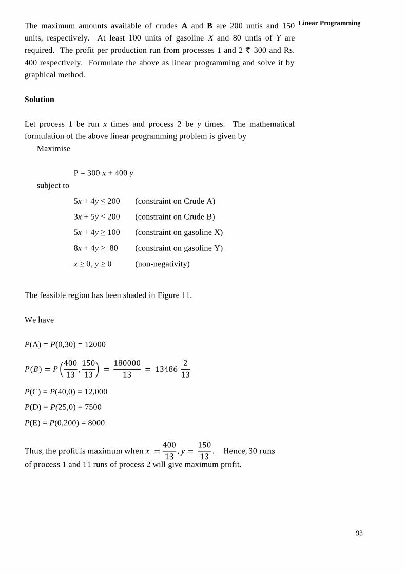
Linear Programming The maximum amounts available of crudes A and B are 200 untis and 150

units, respectively. At least 100 units of gasoline X and 80 untis of Y are

required. The profit per production run from processes 1 and 2 ` 300 and Rs.

400 respectively. Formulate the above as linear programming and solve it by

graphical method.

Solution

Let process 1 be run x times and process 2 be y times. The mathematical

formulation of the above linear programming problem is given by

Maximise

P = 300 x + 400 y

subject to

5x + 4y ≤ 200 (constraint on Crude A)

3x + 5y ≤ 200 (constraint on Crude B)

5x + 4y ≥ 100 (constraint on gasoline X)

8x + 4y ≥ 80 (constraint on gasoline Y)

x ≥ 0, y ≥ 0 (non-negativity)

The feasible region has been shaded in Figure 11.

We have

P(A) = P(0,30) = 12000

P(C) = P(40,0) = 12,000

P(D) = P(25,0) = 7500

P(E) = P(0,200) = 8000

1 and 11 runs of process 2 will give maximum profit.

94

Vectors and Three

Dimensional Geometry

0 10 20 25 30 40 50 60

50

40

30

20

10

5 + 4y = 200

x

3 + 5y = 150

x

5 + 4y = 100

x8+ 4y = 80

x

D(20,0)

E(0,25)

C(40,0)

A(0,30)

x

Y

Figure 11

Remark : The constraint 8x + 4y ≥ 80 does not affect the feasible region, that

is, the constraint 8x + 4y ≥ 80 is a redundant constraint.

No Feasible Solution

In case the solution space or the feasible region is empty, that is, there is no

point which satisfies all the constraints, we say that the linear programming

problem has no feasible solution.

Illustration : We illustrate this in the following linear programming problem.

Maximise

P = 2x + 5y

subject to 5

x + 2y ≤ 10

x ≥ 12

and x≥ 0, y ≥ 0

we draw the feasible region in Fig 12.

10 12 Figure 12

The direction of arrows indicate that the feasible region is empty. Hence, the

given linear programming problem has no feasible solution.

Unbounded solution

Sometimes the feasible region is unbounded. In such cases, the optimal

solution may not exist, because the value of the objective function goes on

increasing in the unbounded region.

B

95

Linear Programming Illustration Let us look at the following illustration.

Maximise

P = 7x + 5y

subject to

2x + 5y ≥ 10

x ≥ 4

y ≥ 3

x ≥ 0, y≥ 0

has no bounded solution.

We draw the feasible region in Fig. 13

y

3

2

0 4 5

Figure 13

The constraint 2x + 5y ≥ 10 is a redundant constraint.

The feasible region is unbounded. Note that the linear programming problem

has no bounded solution.

Chcek Your Progress – 1

1. Best Gift Packs company manufactures two types of gift packs, type A and

type B. Type A requires 5 minutes each for cutting and 10 minutes

assembling it. Type B requires 8 minutes each for cutting and 8 minutes

each for assembling. There are at most 200 minutes available for cutting

and at most 4 hours available for assembling. The profit is ` 50 each for

type A and ` 25 each for type B. How many gift packs of each type should

the company manufacture in order to maximise the profit ?

2. A manufacturer makes two types of furniture, chairs and tables. Both the

products are processed on three machines A1, A2 and A3. Machine A1

requires 3 hrs for a chair and 3 hrs for a table, machine A2 requires 5 hrs

for a chair and 2 hrs for a table and machine A3 requires 2 hrs a chair

and 6 hrs for a table. Maximum time available on machine A1, A2, A3 is

36 hrs, 50 hrs and 60 hrs respectively. Profits are ` 20 per chair and

` 30 per table. Formulate the above as a linear programming problem to

maximise the profit and solve it.

96

Vectors and Three

Dimensional Geometry

3. A manufacturer wishes to produce two types of steel trunks. He has two

machines A and B. For completing, the first type of trunk, he requires 3

hrs on machine A and 2 hrs on machine B whereas the second type of trunk

requires 3 hrs on machine A and 3 hrs on machine B. Machines A and B can

work at the most for 18 hrs and 14 hrs per day respectively. He earns a

profit of `30 and ` 40 per trunk of first type and second type respectively.

How many trunks of each type must he make each day to make

maximum profit? What is his maximum profit?

4. A new businessman wants to make plastic buckets. There are two types

of available plastic bucket making machines. One type of machine

makes 120 buckets a day, occupies 20 square metres and is

operated by 5 men. The corresponding data for second type of

machine is 80 buckets, 24 square metres and 3 men. The available

resources with the businessman are 200 sq. metres and 40 men. How

many machines of each type the manufacturer should buy, so as to

maximise the number of buckets?

5. A producer has 20 and 10 units of labour and capital respectively which

he can use to produce two kinds of goods X and Y. To produce one unit

of goods X, 2 units of capital and 1 unit of labour is required. To

produce one unit of goods Y, 3 units of labour and 1 unit of capital is

required. If X and Y are priced at ` 80 and ` 100 per unit

respectively, how should the producer use his resources to maximize

the total revenue? Solve the problem graphically.

6. A firm has available two kinds of fruit juices – pineapple and

orange juice. These are mixed and the two types of mixtures are

obtained which are sold as soft drinks A and B. One tin of A needs 4

kgs of pineapple juice and 1 kg of orange juice. One tin of B needs 2

kgs of pineapple juice and 3 kgs of orange juice. The firm has

available only 46 kgs of pineapple juice and 24 kgs of orange juice.

Each tin of A and B sold at a profit of ` 4 and ` 2 respectively. How

many tins of A and B should the firm produce to maximise profit?

4.4 COST MINIMISATION

We illustrate the concept by the following example.

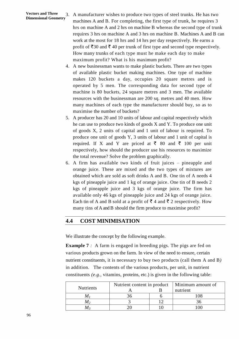
Example 7 : A farm is engaged in breeding pigs. The pigs are fed on

various products grown on the farm. In view of the need to ensure, certain

nutrient constituents, it is necessary to buy two products (call them A and B)

in addition. The contents of the various products, per unit, in nutrient

constituents (e.g., vitamins, proteins, etc.) is given in the following table:

Nutrients Nutrient content in product

A B

Minimum amount of

nutrient

M1 36 6 108

M2 3 12 36

M3 20 10 100

97

Linear Programming The last column of the above table gives the minimum amounts of nutrient

constituients M1, M2, M3 which must given to the pigs. If products A and B cost

` 20 and ` 40 per unit respectively, how much each of these two products

should be bought, so that the total cost is minimised?

Solution

Let x units of A and y units B be purchased. Our goal is to minimise the total

cost

C = 20x + 40y

By using x units of A and y units of B, we shall get 36x + 6y units of

M1 Since we need at least 108 units of M1, we must have

36x + 6y ≥ 108

Similarly for M2 we have 3x + 12y ≥ 36 and for M3 we have 20x + 10y ≥100.

Also, we cannot use negative numbers of x and y. Thus, our problem is

Minimise

C = 20x + 40y

subject to

36x + 6y ≥108

3x + 12y ≥ 36

20x + 10y ≥100

x ≥ 0, y≥ 0

We now draw the constraints on the same graph to obtain the feasible region.

Since x ≥ 0, y ≥ 0, we shall restrict ourself only to the first quadrant. See

Figure 14. We obtain point B by solving 36x + 6y = 108 and 20x + 10y = 100

and point C by solving 3x + 12y = 36 and 20x + 10y = 100. The feasible region

has been shaded.

98

Vectors and Three

Dimensional Geometry

3x +12y =36

36

x + 1

6y =

10

8

20x+ 10y = 100

0 3 5 12

18

10

5

3C(4,2)

D(12,0)

B(2,6)

A(0.18)

y

x

Figure14

We next draw a family of straight lines

with varying values of C. See Figure 15

0 1 2 3 4 5 6 7 8 9 10 11 12 x

6

5

4

3

2

1

y

C = 240C = 200

C = 160C = 120

C = 80C = 40

Equal Cost lines

Direction Increasing Cost

Figure 15

It is clear from here that in order to have least possible cost, we should take

a cost line which intersects the feasible region and is as near to the origin

as possible. Therefore we should consider only the corner points of the

feasible region as possible candidates for least cost.

99

Linear Programming C(A) = C(0, 18) = 720

C(B) = C(2, 6) = 20× 2 + 40× 6 = 280

C(C)=C(4,2)=20×4+40×2= 160

C(D) = C(12, 0) = 240

Minimum cost is obtained at C, that is, for x = 4, y= 2. Minimum possible

cost is `160.

Remark: The procedure for finding least cost is the same as that for the

maximization of profit.

Example 8 A diet for a sick person must contain at least 1400

units of vitamins, 50 units of minerals and 1400 of calories. Two foods

A and B are available at a cost of ` 4 and ` 3 per unit, respectively. If one

unit of A contains 200 units of vitamins, one unit of mineral and 40

calories and one unit of food B contains 100 units of vitamins, two units of

minerals and 40 calories. Find what combination of food be used to have

least cost?

Solution

Let x units of food A and y units of food B be used to give the sick person the

least quantities of vitamins, minerals and calories.

The total cost of the food is C = 4x + 3y. We wish to minimise C.

By consuming x units of A and y units of B, the sick person will get

200x + 100 y units of vitamins. Since the least quantity of vitamin required is

1400, we must have 200x + 100y ≥ 1400

A(0,35)

(E 50,0 )

35

25

B(20,15)

14

0 7 35 50

200x + 100 y = 1400

x +2 y =50

40x + 40 y = 1400

Figure16

Similarly, we must have

Minerals : x + 2y ≥50

Calories : 40x + 40y ≥ 1400

100

Vectors and Three

Dimensional Geometry

Also, since x and y cannot be negative, we must have x ≥0, y ≥0

Thus, the linear programming problem is

Minimise

C = 4x + 3 y

subject to

200 x + 100 y ≥ 1400

x + 2y ≥ 50

40x + 40 y ≥ 1400

and x ≥ 0, y ≥ 0

We draw the feasible region of the above linear programming problem in fig.

16. Note that constraint 200x + 100 y ≥ 1400 is a redundant constraint. The

other two intersect in (20,15).

The corner points of the feasible regions are A(0, 35), B(20,15) and E(50,0).

We find the value of C at each of these corner points.

C(A) = 4(0) + 3(35) = 105

C(B) = 4(20) + 3(15) = 125

C(E) = 4(50) + 3(0) = 200

Thus, least cost is occurs at x = 0, y =35.

Example 9 Every gram of wheat provides 0.1 g of proteins and 0.25 g of

carbohydrates. The corresponding values for rice are 0.05 g and 0.5 g, respectively.

Wheat costs `2 per kg and rice ` 8. The minimum daily requirements of protein and

carbohydrates for an average child are 50 g and 200 g, respectively. In what quanti-

ties should wheat and rice be mixed in the daily diet to provide the minimum daily

requirements of protein and carbohydrates at minimum cost? (The protein and

carbohydrate values given here are fictitious and may be quite different from the

actual values.)

Solution

Let x kg of wheat and y kg of rice be given to the child to give him at least

the minimum requirements of protein and carbohydrates. Then cost of the

food is (2x + 8y) = C (say).

Since one gram wheat contains 0.1 g of proteins, x kg of wheat will contain

(1000 x) (0.1) = 100 x grams of protein.

Similarly, y kg of rice contain (100 y) (0.05) = 50 y grams of protein. Thus,

x kg of wheat and y kg of rice will contain (100 x + 50 y) gms of protein.

101

Linear Programming As the minimum requirement of protein is 50 g, we must have

100x + 50y ≥ 50.

Similarly, for carbohydrate, we must have

(1000x) (0.25) + (1000y) (0.5) ≥ 200

or 250x + 500y ≥ 200

Also, x and y must be non-negative, that is, x ≥ 0, y ≥ 0.

Thus, the linear programming problem is

Minimise

C= 2x + 8y

subject to

100x + 50y ≥ 50

250x + 500y ≥ 200

and x ≥ 0, y ≥ 0.

We draw the feaible region of its problem in Figure 17

A(0,1)

E(0.8,0)

1

0.4

0 ½ 0.8

Figure17

The corner points of the feasible region are A(0,1), B(2/5,1/5) and E(0.8,0).

Let us evaluate C at the conrer points of the feasible region.

C (A) = 2(0) + 8(1) = 8

2 1 12( ) = 2 = 8 = 2.4

5 5 5C B

C (E) = 2(0.8) + 8(0) = 1.6

Thus, the cost is least when x = 0.8, y = 0. The least cost is Rs. 1.60.

2 1,

5 5B

102

Vectors and Three

Dimensional Geometry

Example 10 An animal feed manufacturer produces a compound

mixture from two materials A and B. A costs `2 per kilograms and B,

` 4 per kilogram. Material A is supplied in packs of 25 kilograms and

material B in packs of 50 kilograms. A batch of at least 1,00,000

kilograms of the mixture is to be produced with the specification that at

least 40,000 kilograms of material A, should be used in the manufacture,

which ensures the minimum guaranteed content of the ingredient.

How many packs of A and B should be purchased in order to minimise cost?

Solution

Let x packs of A and y packs of B be purchased in order to meet the

requirement. Our goal is to minimise the total cost. The total cost is

C = 2 25 + 4 50y = 50x + 200y

The constraints are

25x + 50y ≥ 100000

50x ≥ 40000

Therefore, the linear programming problem is

Minimise

C = 50x + 200y

subject to

25x + 50y ≥ 100000

50x ≥ 40000

x ≥ 0, y ≥ 0

We can rewrite the problem as

Minimise

C = 50x + 200y

subject to

x + 2y ≥ 4000

x ≥ 800

x ≥ 0, y ≥ 0

The feasible region of the above linear programming problem is

given in Figure 17

Let us evaluate C at the corner points of the feasible region.

C(A) = 50 800 + 50 1600

= 40000 + 80000 = 120000

C(B) = 50 4000 + 50 0 = 200000

103

Linear Programming

0 800 1000 2000 3000 4000

3000

2000

1000

A (800,1600)

B(4000,0)

Figure 18

Therefore, cost is minimum when x = 800, y = 1600. The minimum possible

cost is Rs. 1,20,000.

Check Your Progress – 2

1. Two tailors, A and B, earn ` 150 and ` 200 per day respectively. A can

stitch 6 shirts and 4 pants while B can stitch 10 shirts and 4 pants per day. How

many days shall each work if it is desired to produce (at least) 60 shirts and 32

pants at a minimum labour cost ? Also calculate the least cost.

2. A dietician mixes together two kinds of food in such a way that the mixture

contains at least 6 units of vitamin A, 7 units of vitamin B, 11 units of vitamin

C and 9 units of vitamin D. The vitamin contents of 1 unit food X and 1 unit

of food Y are given below:

Vitamin A Vitamin B Vitamin C Vitamin D

Food X 1 1 1 2

Food Y 2 1 3 1

One unit of food X costs ` 5, whereas one unit of good Y cost ` 8. Find

the least cost the mixture which will produce the dersired diet. Is

there any redundant constraint ?

3. A diet for a sick person must contain at least 4000 units of vitamins, 50 units of

minerals and 1400 of calories. Two foods, A and B, are available at a cost

of ` 4 and ` 3 per unit respectively. If one unit of A contains 200 units

of vitamin, 1 unit of mineral and 40 calories and one unit of food B contains

100 units of vitamin, 2 units of minerals and 40 calories, find what

combination of foods should be used to have the least cost ? Also calculate

the least cost.

B(4000,0)

104

Vectors and Three

Dimensional Geometry

4. A tailor needs at least 40 large buttons and 60 small buttons. In the market,

buttons are available in boxes or cards. A box contains 6 large and two small

buttons and a card contains 2 large and 4 small buttons. If the cost of a box is

30 paise and card is 20 paise. Find how many boxes and cards should he buy

as to minimise the expenditure ?

4.5 ANSWERS TO CHECK YOUR PROGRESS

1. Type A : x, Type B : y then LPP is

Maximize

P = 50x + 25y

subject to

5x + 8y ≤ 200 [Cutting constraint]

10x + 8y ≤ 240 [Assembly constraint]

x ≥ 0 , y ≥ 0 [Non- negativity]

P(A) = 1200

P (B) = 900

P (C) = 625

P(0) = 0

Thus, profit is maximum when x = 24, y = 0

Maximum profit = Rs. 1200

2. Chairs : x, Tables : y, then LPP is

Maximize

P = 20x + 30y

subject to

3x + 3y ≤ 36 [Machine A1 constraint]

5x + 2y ≤ 50 [Machine A2 constraint]

2x + 6y ≤ 60 [Machine A3 constraint]

x ≥ 0, y ≤ 0 [Non-negativity]

Y

30

25

20

10

010 20 A 30 40 x

CB(8,20)

Figure 19

105

Linear Programming

30

20

10

0 10 20 30 x

Y

3x + 3y = 36

5x + 2y = 50

2x + 6y = 60

D C

B

A

P (A) = 20 (10) + 30(0) = 200

26 10 820 (B) = 20 + 30 =

3 3 3P

P (C) = 20 (3) + 30(9) = 330

P (D) = 20 (10) + 30(0) = 200

P(0) = 20(0) + 30(0) = 0

Thus, profit is maximum

when x = 3, y = 9.

Maximum Profit = Rs. 330

3. First type trunks : x Second type trunks : y

The LPP is

Maximise P = 30 x + 40 y,

subject to

3x + 3y ≤ 18 [Machine A constraint]

2x + 3y ≤ 14 [Machine B constraint]

x ≥ 0, y ≥0 [non-negativity]

P(A) = 180

P(B) =200

P (C) = 560/3

P(O) = 0

Figure 20

106

Vectors and Three

Dimensional Geometry

Thus, profit is maximum when x = 4, y = 2 and maximum profit is Rs. 200.

4. We write the information in the question in tabular form as follows :

First type of

machine (x)

First type of

machine (x)

Constraint

Area 20 (sq. m per

machine)

24 (sq. m per

machine)

≤ 200

Labour 5 (per machine) 3 (per machine) ≤ 40

Buckets 120 (per

machine)

80 (per

machine)

Maximise N

Let x machines of the first type and y machines of the second type be

purchased.

We have to

Maxmise

N = 120 x + 80y

subject to

20 x + 24 y ≤ 200 (Area constraint)

5x + 3y ≤ 40 (Labour constraint)

x ≥ 0, y ≥ 0 ( Non-negativity)

4

6

C

3

B(4,2)

0 3 6 A x

14/3

3 6

x

Figure 21

107

Linear Programming Y

13

25/3

8

6

4

2

0 2 4 6 8 10

x

A(0,25/3)

B(6,10/3)

5x + 3y = 40

20x + 24y =200

C(8,0) Figure 22

The feasible region for the above linear programming problem has been

shaded in the figure.

We find the value of N at the cornor points of the feasible region. We have

25 2,000 2 0, = = 666

3 3 3N (A) = N

10 2960 2N (B) = N 6, = = 986

3 3 3

N (C) = N(8,0) = 960

N (O) = N(0,0) = 0

Thus, the value of N is maximum when x = 6, y = 10/3. As y cannot be in

fraction, we take x = 6, y = 3.

5. We summarise the information given in the question in tabular form as

follows:

Good X Good Y Constraint

Capital 2 1 10

Labour 1 3 20

Revenue 80 100 Maximize R

Let x units of X and y units of Y be produced. The above problem can be

written as

Maxmize

R = 80 x + 100y

subject to

2x + y ≤ 10 (Capital constraint)

x + 3y ≤ 20 (Labour constraint)

x ≥ 0, y ≥ 0 ( Non-negativity)

We shade the feasible region in following figure.

x

108

Vectors and Three

Dimensional Geometry

Y

xC(5,0) 20

B(2,6)

A(0,20/3)

0

10

5

Figure 23

We now check the revenue at corner points of the feasible region.

2R (A) = 80(0) + 100(20/3)= 2000/3 = 666

3

R(B) = 80(2) + 100(6) = 760

R(C) = 80(5) + 100(0) = 400

R(0) = 80(0) + 100(0) = 0

This shows that the revenue is maximum when x = 2 and y = 6

i.e. when 2 units of x and 6 units y are produced and the maximum revenue is

Rs. 760.

6. We summarise the information given in the above question in the

following table.

Drink A Drink B Constraint

Pineapple juice 4(kg per tin) 2(kg per tin) ≤ 46

Orange juice 1(kg per tin) 3(kg per tin) ≤ 24

Profit 4 2 Maximize P

Let x tins of drink A and y tins of drink B be filled up. The above problem

can be written as

Maximise

P = 4x + 2y

Subject to

4x + 2y ≤ 46 (pineabpple juice constraint)

x + 3y ≤ 24 (organge juice constraint)

x ≥ 0, y ≥ 0 (non-negativity)

The feasible region has been shaded. See the following figure.

x

109

Linear Programming Y

23

12

8

4

0 4 8 12 16 20 24 x

4x +

2y =

46

x + 3y = 24

C (23/2,0)

A(0,8)

B(9,5)

Figure 24

We have

P(A) = 4 (0) + 2(8) = 16

P(B) = 4(9) + 2(5) = 46

23( ) 4 + 2(0) = 46

2P C

P(0) = 0

We have maximum profit at B and C. In this case, we say that we have

multiple solutions. In fact, each point on the segment BC gives a profit of

` 46. This is because the segment BC is one of the isoprofit lines.

Check Your Progress 2

1. Suppose tailor A works for x days and tailor B work for y days.

The LPP is

Minimise

C = 150x + 200y

subject to

6x + 10y ≥ 60 [Shirts constraints ]

4x + 4 y ≥ 32 [ Pants constraint]

x ≥ 0, y ≥ 0 [ Non–negativity]

x

110

Vectors and Three

Dimensional Geometry

0 4 8 10

8

4

12

Q(5,3)P

x

R

y

Figure 25

C (P) = 1500

C (Q) = 1350

C( R) = 1600

Thus, cost is least when x =5 and y = 3

2. Food X : x units and Food Y : y units LPP is

P

(5,2)

Q

(1,6)R

S

Y

8

4

3

0 4 6 8 11 12 x

Figure 26

Minimise

C = 5x + 8y

subject to

x + 2 y ≥ 6

x + y ≥ 7

x + 3 y ≥ 11

2 x+ y ≥ 8

x ≥ 0, y ≥ 0

111

Linear Programming

0 10 20 30 35 40 50

Now, C(P) = 55, C (Q) = 41

C(R) = 30, C(S) = 64

Thus, C is least when x = 5, y = 2

least Cost is Rs. 41

The constraint x + 2y ≥ 6 is a redundant constraint.

3. Let x units of food A and y units of food B be used. The LPP is

Minimise

C = 4x + 3y

subject to

200x + 100y ≥ 400 (vitamins constraints)

x + 2 y ≥ 50 (minerals constraints)

40x + 40y ≥ 1400 (calories constraints)

x ≥ 0, y ≥ 0 (non-negativity)

We have

C(P) = 200, C (Q) = 125, C (R) = 110,

C(S) = 120

Thus, C is least when x = 5, y = 30.

40

30

35

20

10

S(0,40)

R(5,30)

Q(20,15)

P(50,0)

Figure 27

x

112

Vectors and Three

Dimensional Geometry

4. Let x boxes and y cards be purchased.

Cost of x boxes is 30x paise and cost of y cards is 20y paise.

Cost incurred by the tailor (in paise ) is 30x + 20y

Number of large buttons obtained from x boses and y cards is 2x + 4y.

According to given condition.

6x + 2y ≥ 40

Number of small buttons obtained from x boxes and y cards is 2x + 4y.

According to the given condition

2x + 4y ≥60

Also, x ≥ 0, y ≥ 0

Thus, the linear programming problem is

Minimize

C = 30 x + 20y [objective function]

subject to

6x + 2y ≥40 [large button constraint]

2 x + 4y ≥ 60 [small button constraint]

x ≥0, y ≥0 [ non-negativity]

We draw the feasible in the following figure.

We now calculate the cost at the corner points of the feasible region.

C(A) = C(0,20) = 30(0) + (20)(20) = 400

C(B) = C(5/2, 55/2) = (30) (5/2) = (20) (55/2) = 75 + 550 = 525

C(D) = C (30,0) = (30)(30) + (20)(0) = 900

Figure 28

Thus, the least cost occurs when the tailor purchases just 20 cards and the least

cost is 400.

0

B(5/2,55/2)

15

A (0,20)

20/3 D(30,0)

³

X

6x + 2y ≥40

2x + 4y ≥ 60

x

113

Linear Programming 4.7 SUMMARY

The unit is about the mathematical discipline of linear programming. In section

4.0, a number of relevant concepts including that of objective function, feasible

region/solution space are introduced. Then the nomenclature ‘linear

programming’ is explained. In section 4.2 the above concepts alongwith some

other relevant concepts are (formally) defined. Section 4.3 explains the two

graphical methods for solving linear programming problems (L.P.P.). viz. (i)

corner point method (ii) iso-profit and iso-cost method. The methods are

explained through a number of examples. Section 4.4 discusses methods of cost

minimisation in context of linear programming problems.

Answers/Solutions to questions/problems/exercises given in various sections of

the unit are available in section 4.5.