
Linear parameter varying controller for a small turboshaft ...1310/... · Linear Parameter Varying...
158
Linear Parameter Varying Controller for a Small Turboshaft Engine A Thesis Presented by Jeffrey Michael Spack to The Department of Electrical & Computer Engineering in partial fulfillment of the requirements for the degree of Master of Science in Electrical Engineering in the field of Control Systems Northeastern University Boston, Massachusetts September 2011
Transcript of Linear parameter varying controller for a small turboshaft ...1310/... · Linear Parameter Varying...
Linear Parameter Varying Controller for a Small
Turboshaft Engine
A Thesis Presented
by
Jeffrey Michael Spack
to
The Department of Electrical & Computer Engineering
in partial fulfillment of the requirementsfor the degree of
Master of Science
in
Electrical Engineering
in the field of
Control Systems
Northeastern UniversityBoston, Massachusetts
September 2011
Linear Parameter Varying Controller for a Small Turboshaft
Engine
by
Jeffrey Michael Spack
Submitted to the Electrical & Computer Engineeringon May 12, 2011, in partial fulfillment of the requirements for the degree of
Master of Science
Abstract
Small turboshaft engine control systems are traditionally single input single output (SISO)and are designed utilizing classical control methods which require extensive gain schedulesresulting in considerable tuning effort. In addition, this method assumes that a system thatis stable at the linearized points will be stable in between the linearized points which may ormay not be true. With a linear parameter varying (LPV) control system, the gain scheduleis inherently built into the controller and the system is guaranteed to be stable betweenlinearizing points as long as the plant depends affinely on a set of time varying parametersthat are available as real time measurements and also vary along a fixed polytope. Anotherbenefit of using an LPV controller in place of a classic SISO controller is that modern robustcontrol techniques can be applied.
A model of a General Electric T700 turboshaft engine and baseline control systemwere developed in Simulink�using a NASA paper written by Mark G. Ballin [1]. Theengine plant was linearized at engine core speed points between 76% and 100% at intervalsof 2%. The LPV power turbine speed controller was developed using linearized plantsderived from the Simulink�model. The LPV controller was then compared to the baselinecontrol system showing performance greater than or equal to the baseline controller with asingle set of weighting functions. The referee transients used to determine a performancecomparison included steps and ramps in power turbine speed reference, helicopter collectiveload disturbances and uncompensated helicopter rotor load disturbances.
This research shows that an LPV controller can be applied to a small turboshaft engineapplication. It is also shown that while the LPV controller is more complex that is shouldtrade well against the traditional SISO methods based on tuning effort and performance.
Thesis Advisor: Professor Mario Sznaier
2

This thesis is dedicated to my wife and family, Constance, Penelope and Eleni.
Without their love, support and sacrifice my graduate coursework and research
would not have been achievable.
3

Acknowledgments
I would like to thank my advisor Professor Mario Sznaier whose guidance provided
me the necessary tools to complete this research.
I would also like to thank Dave Gutz, who provided great insight into making this
research applicable to a real world application, and my other colleagues at GE who
had to work around with my irregular work schedule and frequently fill in for me when
I was unavailable. The support from the GE Lynn Controls Department management
team was invaluable in allowing me to take the necessary time to complete my degree.
My degree was sponsored by the General Electric Company through the Advanced
Courses in Engineering, under the supervision of Tyler Hooper.
4
Contents
1 Introduction 21
1.1 Background . . . . . . . . . . . . . . . . . . . . . . . . . . . . . . . . 21
1.2 Scope . . . . . . . . . . . . . . . . . . . . . . . . . . . . . . . . . . . 24
2 Engine Control System 25
3 Engine Model 27
3.1 Engine Model Assumptions . . . . . . . . . . . . . . . . . . . . . . . 28
3.2 Engine Model Tools . . . . . . . . . . . . . . . . . . . . . . . . . . . 28
3.3 Engine Model Architecture . . . . . . . . . . . . . . . . . . . . . . . 28
3.4 Engine Model Validation . . . . . . . . . . . . . . . . . . . . . . . . 40
3.5 Engine Model Linearization . . . . . . . . . . . . . . . . . . . . . . . 42
4 Load Model 48
4.1 Load Model Assumptions . . . . . . . . . . . . . . . . . . . . . . . . 48
4.2 Load Model Architecture . . . . . . . . . . . . . . . . . . . . . . . . 49
5 Engine Baseline Control System Model 52
5.1 Baseline Controller Assumptions . . . . . . . . . . . . . . . . . . . . . 53
5.2 Baseline Controller Tools . . . . . . . . . . . . . . . . . . . . . . . . 54
5.3 Baseline Controller Architecture . . . . . . . . . . . . . . . . . . . . 54
5.4 Baseline Controller Validation . . . . . . . . . . . . . . . . . . . . . . 61
6 Linear Parameter Varying (LPV) Control Theory 64
5
6.1 Classical Approach . . . . . . . . . . . . . . . . . . . . . . . . . . . . 64
6.2 LPV Approach . . . . . . . . . . . . . . . . . . . . . . . . . . . . . . 65
7 LPV Controller Design 71
7.1 LPV Controller Assumptions . . . . . . . . . . . . . . . . . . . . . . 71
7.2 LPV Controller Tools . . . . . . . . . . . . . . . . . . . . . . . . . . 71
7.2.1 Changes to LMI toolset to deal with polytopic model . . . . . 72
7.3 LPV Controller Architecture . . . . . . . . . . . . . . . . . . . . . . . 72
7.4 LPV Controller Validation . . . . . . . . . . . . . . . . . . . . . . . . 80
7.4.1 Comparison of baseline controller versus LPV controller . . . . 81
8 Conclusions 90
8.1 Future Work . . . . . . . . . . . . . . . . . . . . . . . . . . . . . . . . 91
A Engine Model Diagrams 92
B Engine Model Constants 97
C Engine Model Schedules 99
D Fuel Control Model Diagrams 118
E Fuel Control Constants 123
F Fuel Control Schedules 124
G Matlab�Code 136
G.1 LMI Toolbox Commands [2] . . . . . . . . . . . . . . . . . . . . . . . 136
G.2 Linearization Scripts . . . . . . . . . . . . . . . . . . . . . . . . . . . 140
G.3 Changes to LMI toolset code . . . . . . . . . . . . . . . . . . . . . . . 145
G.4 LPV Controller . . . . . . . . . . . . . . . . . . . . . . . . . . . . . . 147
G.4.1 Modified Plant Setup . . . . . . . . . . . . . . . . . . . . . . . 147
G.4.2 LPV Controller Design . . . . . . . . . . . . . . . . . . . . . . 148
G.4.3 LPV Controller Linear Simulation . . . . . . . . . . . . . . . . 149
6

G.4.4 Write Trajectory File . . . . . . . . . . . . . . . . . . . . . . . 149
G.4.5 Linear Simulation Input Function . . . . . . . . . . . . . . . . 150
G.4.6 LPV Controller s-function . . . . . . . . . . . . . . . . . . . . 150
H Results 152
H.1 Linear Plants . . . . . . . . . . . . . . . . . . . . . . . . . . . . . . . 152
7
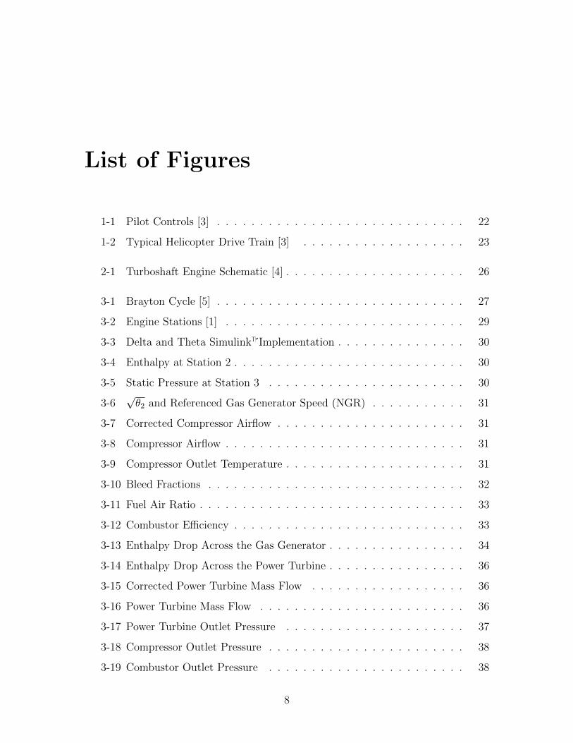
List of Figures
1-1 Pilot Controls [3] . . . . . . . . . . . . . . . . . . . . . . . . . . . . . 22
1-2 Typical Helicopter Drive Train [3] . . . . . . . . . . . . . . . . . . . 23
2-1 Turboshaft Engine Schematic [4] . . . . . . . . . . . . . . . . . . . . . 26
3-1 Brayton Cycle [5] . . . . . . . . . . . . . . . . . . . . . . . . . . . . . 27
3-2 Engine Stations [1] . . . . . . . . . . . . . . . . . . . . . . . . . . . . 29
3-3 Delta and Theta Simulink�Implementation . . . . . . . . . . . . . . . 30
3-4 Enthalpy at Station 2 . . . . . . . . . . . . . . . . . . . . . . . . . . . 30
3-5 Static Pressure at Station 3 . . . . . . . . . . . . . . . . . . . . . . . 30
3-6√θ2 and Referenced Gas Generator Speed (NGR) . . . . . . . . . . . 31
3-7 Corrected Compressor Airflow . . . . . . . . . . . . . . . . . . . . . . 31
3-8 Compressor Airflow . . . . . . . . . . . . . . . . . . . . . . . . . . . . 31
3-9 Compressor Outlet Temperature . . . . . . . . . . . . . . . . . . . . . 31
3-10 Bleed Fractions . . . . . . . . . . . . . . . . . . . . . . . . . . . . . . 32
3-11 Fuel Air Ratio . . . . . . . . . . . . . . . . . . . . . . . . . . . . . . . 33
3-12 Combustor Efficiency . . . . . . . . . . . . . . . . . . . . . . . . . . . 33
3-13 Enthalpy Drop Across the Gas Generator . . . . . . . . . . . . . . . . 34
3-14 Enthalpy Drop Across the Power Turbine . . . . . . . . . . . . . . . . 36
3-15 Corrected Power Turbine Mass Flow . . . . . . . . . . . . . . . . . . 36
3-16 Power Turbine Mass Flow . . . . . . . . . . . . . . . . . . . . . . . . 36
3-17 Power Turbine Outlet Pressure . . . . . . . . . . . . . . . . . . . . . 37
3-18 Compressor Outlet Pressure . . . . . . . . . . . . . . . . . . . . . . . 38
3-19 Combustor Outlet Pressure . . . . . . . . . . . . . . . . . . . . . . . 38
8
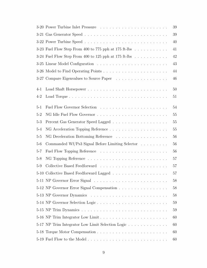
3-20 Power Turbine Inlet Pressure . . . . . . . . . . . . . . . . . . . . . . 39
3-21 Gas Generator Speed . . . . . . . . . . . . . . . . . . . . . . . . . . . 39
3-22 Power Turbine Speed . . . . . . . . . . . . . . . . . . . . . . . . . . . 40
3-23 Fuel Flow Step From 400 to 775 pph at 175 ft-lbs . . . . . . . . . . . 41
3-24 Fuel Flow Step From 400 to 125 pph at 175 ft-lbs . . . . . . . . . . . 42
3-25 Linear Model Configuration . . . . . . . . . . . . . . . . . . . . . . . 43
3-26 Model to Find Operating Points . . . . . . . . . . . . . . . . . . . . . 44
3-27 Compare Eigenvalues to Source Paper . . . . . . . . . . . . . . . . . 46
4-1 Load Shaft Horsepower . . . . . . . . . . . . . . . . . . . . . . . . . . 50
4-2 Load Torque . . . . . . . . . . . . . . . . . . . . . . . . . . . . . . . . 51
5-1 Fuel Flow Governor Selection . . . . . . . . . . . . . . . . . . . . . . 54
5-2 NG Idle Fuel Flow Governor . . . . . . . . . . . . . . . . . . . . . . . 55
5-3 Percent Gas Generator Speed Lagged . . . . . . . . . . . . . . . . . . 55
5-4 NG Acceleration Topping Reference . . . . . . . . . . . . . . . . . . . 55
5-5 NG Deceleration Bottoming Reference . . . . . . . . . . . . . . . . . 56
5-6 Commanded Wf/Ps3 Signal Before Limiting Selector . . . . . . . . . 56
5-7 Fuel Flow Topping Reference . . . . . . . . . . . . . . . . . . . . . . 56
5-8 NG Topping Reference . . . . . . . . . . . . . . . . . . . . . . . . . . 57
5-9 Collective Based Feedforward . . . . . . . . . . . . . . . . . . . . . . 57
5-10 Collective Based Feedforward Lagged . . . . . . . . . . . . . . . . . . 57
5-11 NP Governor Error Signal . . . . . . . . . . . . . . . . . . . . . . . . 58
5-12 NP Governor Error Signal Compensation . . . . . . . . . . . . . . . . 58
5-13 NP Governor Dynamics . . . . . . . . . . . . . . . . . . . . . . . . . 58
5-14 NP Governor Selection Logic . . . . . . . . . . . . . . . . . . . . . . . 59
5-15 NP Trim Dynamics . . . . . . . . . . . . . . . . . . . . . . . . . . . . 59
5-16 NP Trim Integrator Low Limit . . . . . . . . . . . . . . . . . . . . . . 60
5-17 NP Trim Integrator Low Limit Selection Logic . . . . . . . . . . . . . 60
5-18 Torque Motor Compensation . . . . . . . . . . . . . . . . . . . . . . . 60
5-19 Fuel Flow to the Model . . . . . . . . . . . . . . . . . . . . . . . . . . 60
9
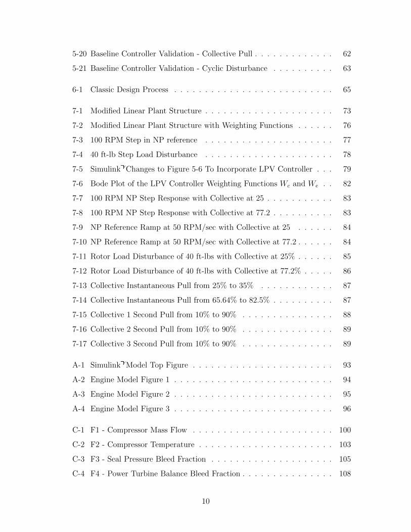
5-20 Baseline Controller Validation - Collective Pull . . . . . . . . . . . . . 62
5-21 Baseline Controller Validation - Cyclic Disturbance . . . . . . . . . . 63
6-1 Classic Design Process . . . . . . . . . . . . . . . . . . . . . . . . . . 65
7-1 Modified Linear Plant Structure . . . . . . . . . . . . . . . . . . . . . 73
7-2 Modified Linear Plant Structure with Weighting Functions . . . . . . 76
7-3 100 RPM Step in NP reference . . . . . . . . . . . . . . . . . . . . . 77
7-4 40 ft-lb Step Load Disturbance . . . . . . . . . . . . . . . . . . . . . 78
7-5 Simulink�Changes to Figure 5-6 To Incorporate LPV Controller . . . 79
7-6 Bode Plot of the LPV Controller Weighting Functions Wc and We . . 82
7-7 100 RPM NP Step Response with Collective at 25 . . . . . . . . . . . 83
7-8 100 RPM NP Step Response with Collective at 77.2 . . . . . . . . . . 83
7-9 NP Reference Ramp at 50 RPM/sec with Collective at 25 . . . . . . 84
7-10 NP Reference Ramp at 50 RPM/sec with Collective at 77.2 . . . . . . 84
7-11 Rotor Load Disturbance of 40 ft-lbs with Collective at 25% . . . . . . 85
7-12 Rotor Load Disturbance of 40 ft-lbs with Collective at 77.2% . . . . . 86
7-13 Collective Instantaneous Pull from 25% to 35% . . . . . . . . . . . . 87
7-14 Collective Instantaneous Pull from 65.64% to 82.5% . . . . . . . . . . 87
7-15 Collective 1 Second Pull from 10% to 90% . . . . . . . . . . . . . . . 88
7-16 Collective 2 Second Pull from 10% to 90% . . . . . . . . . . . . . . . 89
7-17 Collective 3 Second Pull from 10% to 90% . . . . . . . . . . . . . . . 89
A-1 Simulink�Model Top Figure . . . . . . . . . . . . . . . . . . . . . . . 93
A-2 Engine Model Figure 1 . . . . . . . . . . . . . . . . . . . . . . . . . . 94
A-3 Engine Model Figure 2 . . . . . . . . . . . . . . . . . . . . . . . . . . 95
A-4 Engine Model Figure 3 . . . . . . . . . . . . . . . . . . . . . . . . . . 96
C-1 F1 - Compressor Mass Flow . . . . . . . . . . . . . . . . . . . . . . . 100
C-2 F2 - Compressor Temperature . . . . . . . . . . . . . . . . . . . . . . 103
C-3 F3 - Seal Pressure Bleed Fraction . . . . . . . . . . . . . . . . . . . . 105
C-4 F4 - Power Turbine Balance Bleed Fraction . . . . . . . . . . . . . . . 108
10
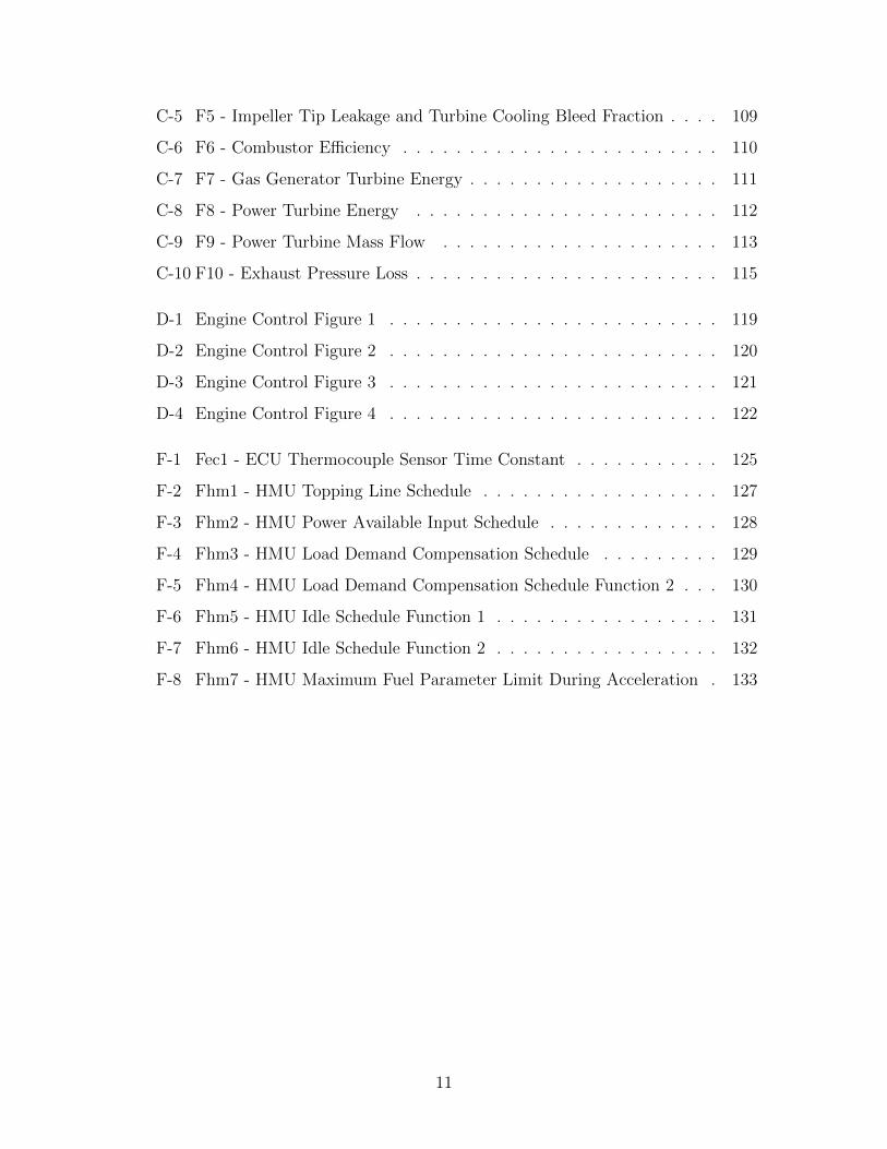
C-5 F5 - Impeller Tip Leakage and Turbine Cooling Bleed Fraction . . . . 109
C-6 F6 - Combustor Efficiency . . . . . . . . . . . . . . . . . . . . . . . . 110
C-7 F7 - Gas Generator Turbine Energy . . . . . . . . . . . . . . . . . . . 111
C-8 F8 - Power Turbine Energy . . . . . . . . . . . . . . . . . . . . . . . 112
C-9 F9 - Power Turbine Mass Flow . . . . . . . . . . . . . . . . . . . . . 113
C-10 F10 - Exhaust Pressure Loss . . . . . . . . . . . . . . . . . . . . . . . 115
D-1 Engine Control Figure 1 . . . . . . . . . . . . . . . . . . . . . . . . . 119
D-2 Engine Control Figure 2 . . . . . . . . . . . . . . . . . . . . . . . . . 120
D-3 Engine Control Figure 3 . . . . . . . . . . . . . . . . . . . . . . . . . 121
D-4 Engine Control Figure 4 . . . . . . . . . . . . . . . . . . . . . . . . . 122
F-1 Fec1 - ECU Thermocouple Sensor Time Constant . . . . . . . . . . . 125
F-2 Fhm1 - HMU Topping Line Schedule . . . . . . . . . . . . . . . . . . 127
F-3 Fhm2 - HMU Power Available Input Schedule . . . . . . . . . . . . . 128
F-4 Fhm3 - HMU Load Demand Compensation Schedule . . . . . . . . . 129
F-5 Fhm4 - HMU Load Demand Compensation Schedule Function 2 . . . 130
F-6 Fhm5 - HMU Idle Schedule Function 1 . . . . . . . . . . . . . . . . . 131
F-7 Fhm6 - HMU Idle Schedule Function 2 . . . . . . . . . . . . . . . . . 132
F-8 Fhm7 - HMU Maximum Fuel Parameter Limit During Acceleration . 133
11
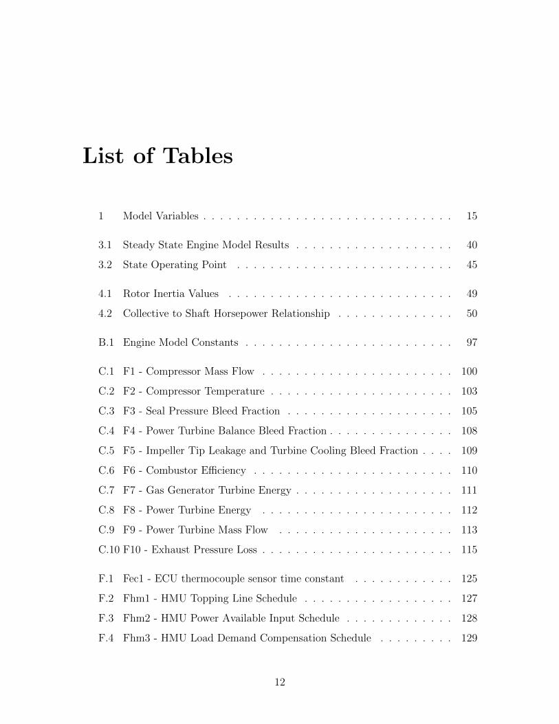
List of Tables
1 Model Variables . . . . . . . . . . . . . . . . . . . . . . . . . . . . . . 15
3.1 Steady State Engine Model Results . . . . . . . . . . . . . . . . . . . 40
3.2 State Operating Point . . . . . . . . . . . . . . . . . . . . . . . . . . 45
4.1 Rotor Inertia Values . . . . . . . . . . . . . . . . . . . . . . . . . . . 49
4.2 Collective to Shaft Horsepower Relationship . . . . . . . . . . . . . . 50
B.1 Engine Model Constants . . . . . . . . . . . . . . . . . . . . . . . . . 97
C.1 F1 - Compressor Mass Flow . . . . . . . . . . . . . . . . . . . . . . . 100
C.2 F2 - Compressor Temperature . . . . . . . . . . . . . . . . . . . . . . 103
C.3 F3 - Seal Pressure Bleed Fraction . . . . . . . . . . . . . . . . . . . . 105
C.4 F4 - Power Turbine Balance Bleed Fraction . . . . . . . . . . . . . . . 108
C.5 F5 - Impeller Tip Leakage and Turbine Cooling Bleed Fraction . . . . 109
C.6 F6 - Combustor Efficiency . . . . . . . . . . . . . . . . . . . . . . . . 110
C.7 F7 - Gas Generator Turbine Energy . . . . . . . . . . . . . . . . . . . 111
C.8 F8 - Power Turbine Energy . . . . . . . . . . . . . . . . . . . . . . . 112
C.9 F9 - Power Turbine Mass Flow . . . . . . . . . . . . . . . . . . . . . 113
C.10 F10 - Exhaust Pressure Loss . . . . . . . . . . . . . . . . . . . . . . . 115
F.1 Fec1 - ECU thermocouple sensor time constant . . . . . . . . . . . . 125
F.2 Fhm1 - HMU Topping Line Schedule . . . . . . . . . . . . . . . . . . 127
F.3 Fhm2 - HMU Power Available Input Schedule . . . . . . . . . . . . . 128
F.4 Fhm3 - HMU Load Demand Compensation Schedule . . . . . . . . . 129
12
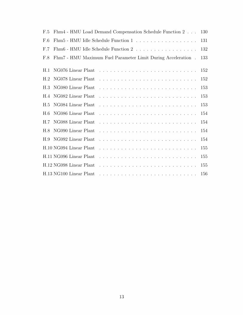
F.5 Fhm4 - HMU Load Demand Compensation Schedule Function 2 . . . 130
F.6 Fhm5 - HMU Idle Schedule Function 1 . . . . . . . . . . . . . . . . . 131
F.7 Fhm6 - HMU Idle Schedule Function 2 . . . . . . . . . . . . . . . . . 132
F.8 Fhm7 - HMU Maximum Fuel Parameter Limit During Acceleration . 133
H.1 NG076 Linear Plant . . . . . . . . . . . . . . . . . . . . . . . . . . . 152
H.2 NG078 Linear Plant . . . . . . . . . . . . . . . . . . . . . . . . . . . 152
H.3 NG080 Linear Plant . . . . . . . . . . . . . . . . . . . . . . . . . . . 153
H.4 NG082 Linear Plant . . . . . . . . . . . . . . . . . . . . . . . . . . . 153
H.5 NG084 Linear Plant . . . . . . . . . . . . . . . . . . . . . . . . . . . 153
H.6 NG086 Linear Plant . . . . . . . . . . . . . . . . . . . . . . . . . . . 154
H.7 NG088 Linear Plant . . . . . . . . . . . . . . . . . . . . . . . . . . . 154
H.8 NG090 Linear Plant . . . . . . . . . . . . . . . . . . . . . . . . . . . 154
H.9 NG092 Linear Plant . . . . . . . . . . . . . . . . . . . . . . . . . . . 154
H.10 NG094 Linear Plant . . . . . . . . . . . . . . . . . . . . . . . . . . . 155
H.11 NG096 Linear Plant . . . . . . . . . . . . . . . . . . . . . . . . . . . 155
H.12 NG098 Linear Plant . . . . . . . . . . . . . . . . . . . . . . . . . . . 155
H.13 NG100 Linear Plant . . . . . . . . . . . . . . . . . . . . . . . . . . . 156
13
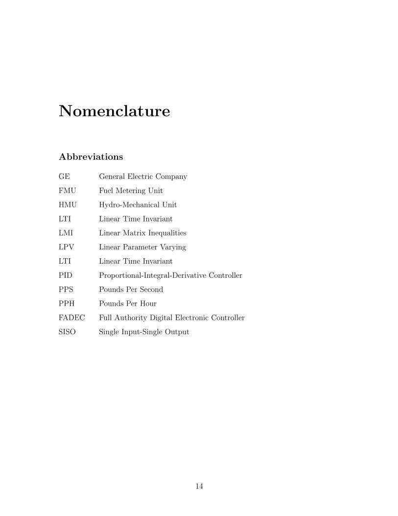
Nomenclature
Abbreviations
GE General Electric Company
FMU Fuel Metering Unit
HMU Hydro-Mechanical Unit
LTI Linear Time Invariant
LMI Linear Matrix Inequalities
LPV Linear Parameter Varying
LTI Linear Time Invariant
PID Proportional-Integral-Derivative Controller
PPS Pounds Per Second
PPH Pounds Per Hour
FADEC Full Authority Digital Electronic Controller
SISO Single Input-Single Output
14
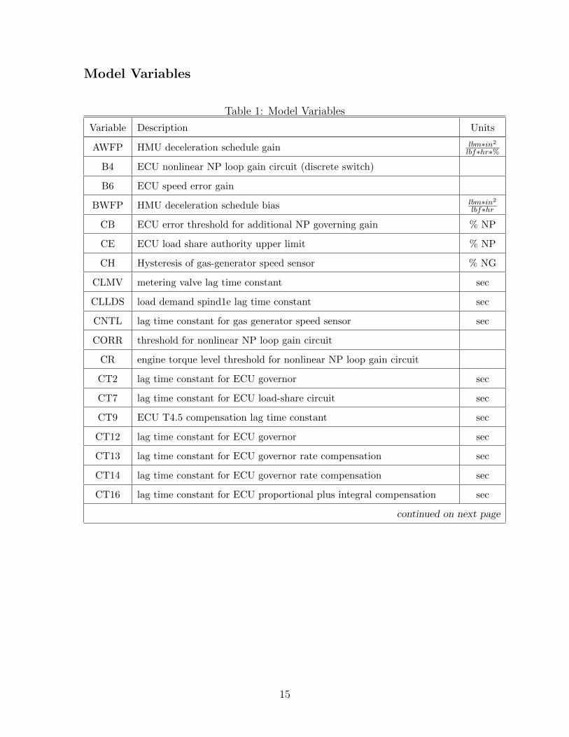
Model Variables
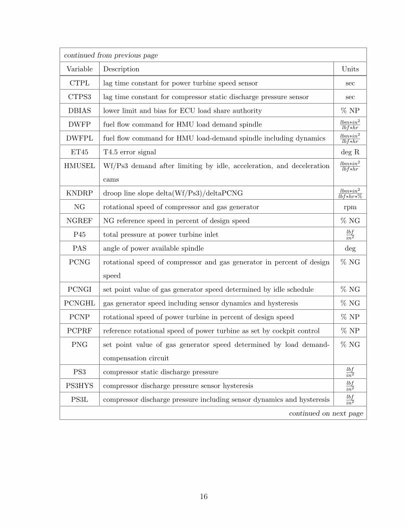
Table 1: Model Variables
Variable Description Units
AWFP HMU deceleration schedule gain lbm∗in2
lbf∗hr∗%
B4 ECU nonlinear NP loop gain circuit (discrete switch)
B6 ECU speed error gain
BWFP HMU deceleration schedule bias lbm∗in2
lbf∗hr
CB ECU error threshold for additional NP governing gain % NP
CE ECU load share authority upper limit % NP
CH Hysteresis of gas-generator speed sensor % NG
CLMV metering valve lag time constant sec
CLLDS load demand spind1e lag time constant sec
CNTL lag time constant for gas generator speed sensor sec
CORR threshold for nonlinear NP loop gain circuit
CR engine torque level threshold for nonlinear NP loop gain circuit
CT2 lag time constant for ECU governor sec
CT7 lag time constant for ECU load-share circuit sec
CT9 ECU T4.5 compensation lag time constant sec
CT12 lag time constant for ECU governor sec
CT13 lag time constant for ECU governor rate compensation sec
CT14 lag time constant for ECU governor rate compensation sec
CT16 lag time constant for ECU proportional plus integral compensation sec
continued on next page
15
continued from previous page
Variable Description Units
CTPL lag time constant for power turbine speed sensor sec
CTPS3 lag time constant for compressor static discharge pressure sensor sec
DBIAS lower limit and bias for ECU load share authority % NP
DWFP fuel flow command for HMU load demand spindle lbm∗in2
lbf∗hr
DWFPL fuel flow command for HMU load-demand spindle including dynamics lbm∗in2
lbf∗hr
ET45 T4.5 error signal deg R
HMUSEL Wf/Ps3 demand after limiting by idle, acceleration, and deceleration
cams
lbm∗in2
lbf∗hr
KNDRP droop line slope delta(Wf/Ps3)/deltaPCNG lbm∗in2
lbf∗hr∗%
NG rotational speed of compressor and gas generator rpm
NGREF NG reference speed in percent of design speed % NG
P45 total pressure at power turbine inlet lbfin2
PAS angle of power available spindle deg
PCNG rotational speed of compressor and gas generator in percent of design
speed
% NG
PCNGI set point value of gas generator speed determined by idle schedule % NG
PCNGHL gas generator speed including sensor dynamics and hysteresis % NG
PCNP rotational speed of power turbine in percent of design speed % NP
PCPRF reference rotational speed of power turbine as set by cockpit control % NP
PNG set point value of gas generator speed determined by load demand-
compensation circuit
% NG
PS3 compressor static discharge pressure lbfin2
PS3HYS compressor discharge pressure sensor hysteresis lbfin2
PS3L compressor discharge pressure including sensor dynamics and hysteresis lbfin2
continued on next page
16
continued from previous page
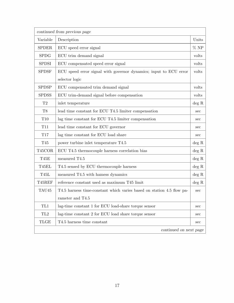
Variable Description Units
SPDER ECU speed error signal % NP
SPDG ECU trim demand signal volts
SPDSI ECU compensated speed error signal volts
SPDSF ECU speed error signal with governor dynamics; input to ECU error
selector logic
volts
SPDSP ECU compensated trim demand signal volts
SPDSS ECU trim-demand signal before compensation volts
T2 inlet temperature deg R
T8 lead time constant for ECU T4.5 limiter compensation sec
T10 lag time constant for ECU T4.5 limiter compensation sec
T11 lead time constant for ECU governor sec
T17 lag time constant for ECU load share sec
T45 power turbine inlet temperature T4.5 deg R
T45COR ECU T4.5 thermocouple harness correlation bias deg R
T45E measured T4.5 deg R
T45EL T4.5 sensed by ECU thermocouple harness deg R
T45L measured T4.5 with hamess dynamics deg R
T45REF reference constant used as maximum T45 limit deg R
TAU45 T4.5 harness time-constant which varies based on station 4.5 flow pa-
rameter and T4.5
sec
TL1 lag-time constant 1 for ECU load-share torque sensor sec
TL2 lag-time constant 2 for ECU load share torque sensor sec
TLGE T4.5 harness time constant sec
continued on next page
17
continued from previous page
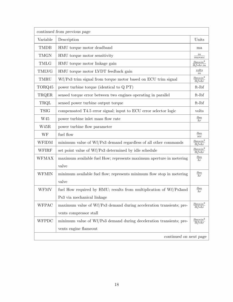
Variable Description Units
TMDB HMU torque motor deadband ma
TMGN HMU torque motor sensitivity inma∗sec
TMLG HMU torque motor linkage gain lbm∗in2
lbf∗hr.in
TMLVG HMU torque motor LVDT feedback gain voltsin
TMRU Wf/Ps3 trim signal from torque motor based on ECU trim signal lbm∗in2
lbf∗hr
TORQ45 power turbine torque (identical to Q PT) ft-lbf
TRQER sensed torque error between two engines operating in parallel ft-lbf
TRQL sensed power turbine output torque ft-lbf
TSIG compensated T4.5 error signal; input to ECU error selector logic volts
W45 power turbine inlet mass flow rate lbmhr
W45R power turbine flow parameter
WF fuel flow lbmsec
WFIDM minimum value of Wf/Ps3 demand regardless of all other commands lbm∗in2
lbf∗hr
WFIRF set point value of Wf/Ps3 determined by idle schedule lbm∗in2
lbf∗hr
WFMAX maximum available fuel How; represents maximum aperture in metering
valve
lbmhr
WFMIN minimum available fuel flow; represents minimum flow stop in metering
valve
lbmhr
WFMV fuel How required by HMU; results from multiplication of Wf/Ps3and
Ps3 via mechanical linkage
lbmhr
WFPAC maximum value of Wf/Ps3 demand during acceleration transients; pre-
vents compressor stall
lbm∗in2
lbf∗hr
WFPDC minimum value of Wf/Ps3 demand during deceleration transients; pre-
vents engine flameout
lbm∗in2
lbf∗hr
continued on next page
18
continued from previous page
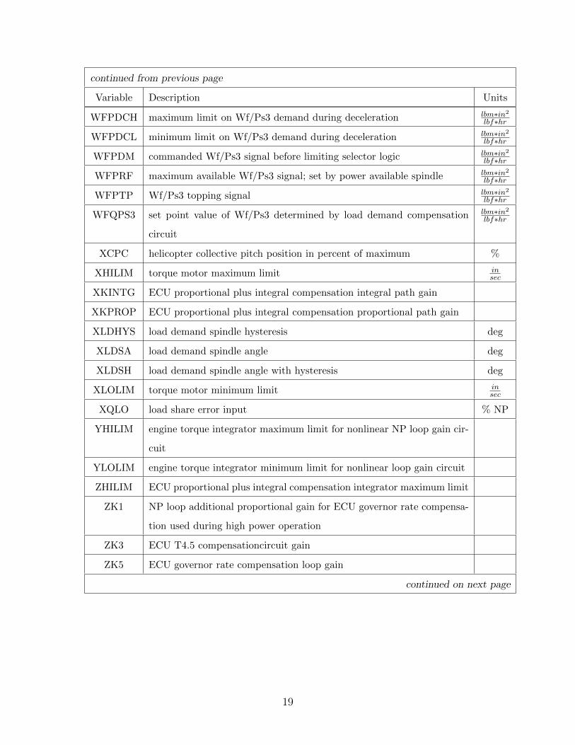
Variable Description Units
WFPDCH maximum limit on Wf/Ps3 demand during deceleration lbm∗in2
lbf∗hr
WFPDCL minimum limit on Wf/Ps3 demand during deceleration lbm∗in2
lbf∗hr
WFPDM commanded Wf/Ps3 signal before limiting selector logic lbm∗in2
lbf∗hr
WFPRF maximum available Wf/Ps3 signal; set by power available spindle lbm∗in2
lbf∗hr
WFPTP Wf/Ps3 topping signal lbm∗in2
lbf∗hr
WFQPS3 set point value of Wf/Ps3 determined by load demand compensation
circuit
lbm∗in2
lbf∗hr
XCPC helicopter collective pitch position in percent of maximum %
XHILIM torque motor maximum limit insec
XKINTG ECU proportional plus integral compensation integral path gain
XKPROP ECU proportional plus integral compensation proportional path gain
XLDHYS load demand spindle hysteresis deg
XLDSA load demand spindle angle deg
XLDSH load demand spindle angle with hysteresis deg
XLOLIM torque motor minimum limit insec
XQLO load share error input % NP
YHILIM engine torque integrator maximum limit for nonlinear NP loop gain cir-
cuit
YLOLIM engine torque integrator minimum limit for nonlinear loop gain circuit
ZHILIM ECU proportional plus integral compensation integrator maximum limit
ZK1 NP loop additional proportional gain for ECU governor rate compensa-
tion used during high power operation
ZK3 ECU T4.5 compensationcircuit gain
ZK5 ECU governor rate compensation loop gain
continued on next page
19
continued from previous page
Variable Description Units
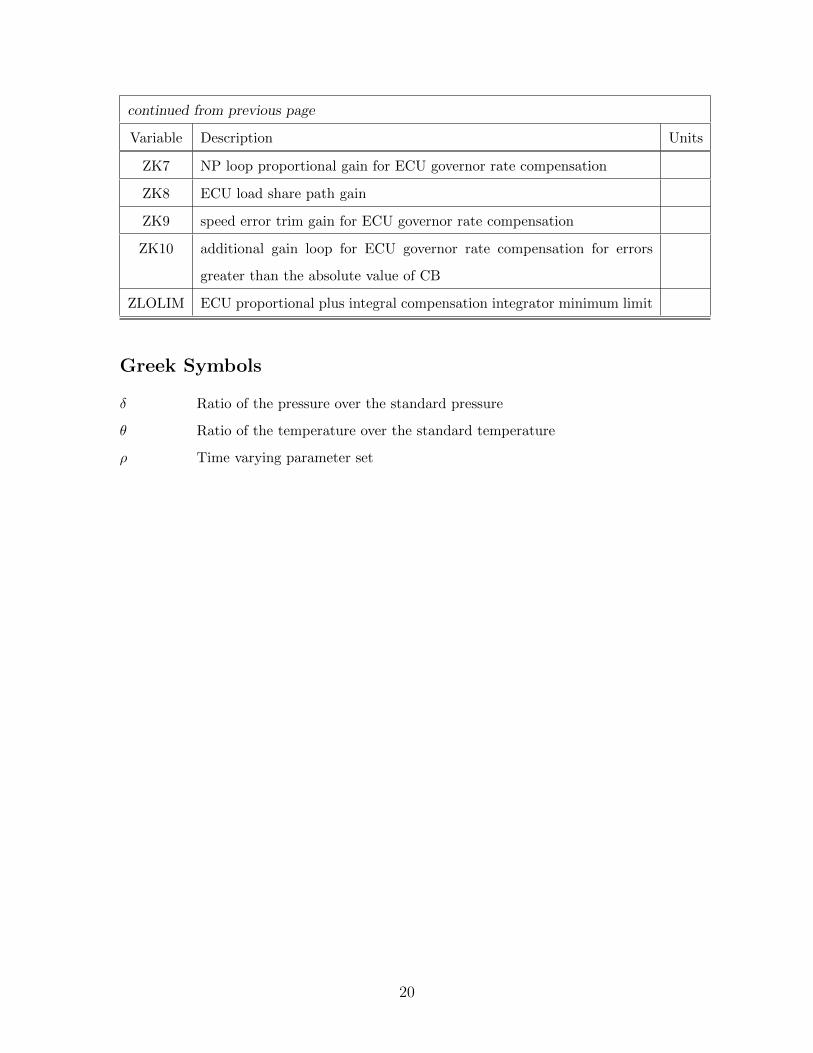
ZK7 NP loop proportional gain for ECU governor rate compensation
ZK8 ECU load share path gain
ZK9 speed error trim gain for ECU governor rate compensation
ZK10 additional gain loop for ECU governor rate compensation for errors
greater than the absolute value of CB
ZLOLIM ECU proportional plus integral compensation integrator minimum limit
Greek Symbols
δ Ratio of the pressure over the standard pressure
θ Ratio of the temperature over the standard temperature
ρ Time varying parameter set
20
Chapter 1
Introduction
Classical linear single input-single output (SISO) controllers commonly used in helicopter
engine controls typically require extensive tuning and require additional margin between
linearized points for a reasonable assurance of stability. A linear parameter varying (LPV)
controller design provides gained scheduled controller that is stable in between plant lin-
earizing points as long as the plant satisfies a few assumptions:
1. the model depends affinely on a set of time varying parameters
2. the time varying parameters are available as real time measurements
3. the time-varying parameters range within a fixed polytope
Another benefit to an LPV controller is that the extensive tuning required for SISO
controls is significantly reduced. This research produced a controller that performed as well
or better than the baseline controller with a single set of weighting functions.
The downside to a LPV controller is that the complexity, when compared against the
baseline SISO controller[1], is increased. However, the reasonable assurance of stability
between linearized points and decreased tuning effort should trade well against the effort
and cost required to implement a more complex controller in a production environment.
1.1 Background
Small turboshaft engines are typically used for rotor craft, turbo propeller fixed wing aircraft
and large marine applications. In this research, the focus is on a model of a GE T700 turbo
21
shaft engine which is primarily used for rotor craft applications namely the Sikorsky UH-
60A Blackhawk. The Blackhawk is configured as a two engine system where both engines
feed a main gear box which drives the main and tail rotors. The main rotor of a helicopter
provides lift and directional control. The tail rotor counteracts the force applied by the
main rotor that pushes the helicopter body in the opposite direction of the main rotor. The
tail rotor also acts as a rudder to steer the helicopter left and right [3].
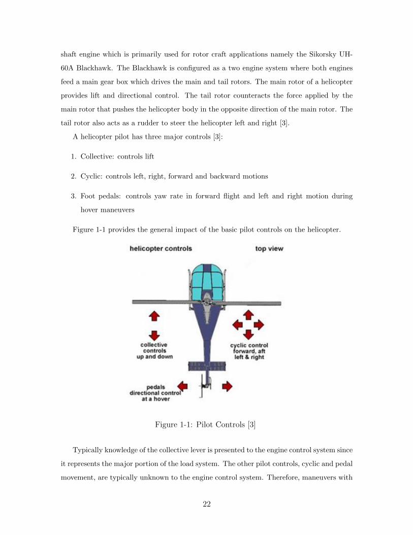
A helicopter pilot has three major controls [3]:
1. Collective: controls lift
2. Cyclic: controls left, right, forward and backward motions
3. Foot pedals: controls yaw rate in forward flight and left and right motion during
hover maneuvers
Figure 1-1 provides the general impact of the basic pilot controls on the helicopter.
Figure 1-1: Pilot Controls [3]
Typically knowledge of the collective lever is presented to the engine control system since
it represents the major portion of the load system. The other pilot controls, cyclic and pedal
movement, are typically unknown to the engine control system. Therefore, maneuvers with
22
significant cyclic and/or pedal movement without significant collective movement rely solely
on the power turbine speed governor while maneuvers with significant collective movement
are typically assisted by open loop anticipation logic.
Rotor craft in general present a complex controls problem for the engine control system
designer due to the integration with the helicopter. Since the engines are directly connected
to the main and tail rotors through the transmission the dynamics of the rotor system must
be included in the governor design. One of the most important requirements for the engine
control system is to keep the main rotor speed close to the datum under varying load con-
ditions while respecting several boundary conditions. Deviations below the datum is called
rotor “droop” and deviations above the datum are called rotor “upspeed” or “overshoot”.
Both are not desirable, too much rotor droop can lead to a unrecoverable loss of lift and
too much overshoot could lead to damage to the main gear box both of which can result in
loss of the aircraft.
The major boundary conditions that the engine control system must respect are: engine
acceleration limits, engine deceleration limits, maximum gas generator speed, minimum gas
generator speed, gas generator turbine temperature limits and engine fuel flow limits. In
addition, the engine control system must have good handling qualities at the aircraft level
such as avoiding torque reversals during engine acceleration.
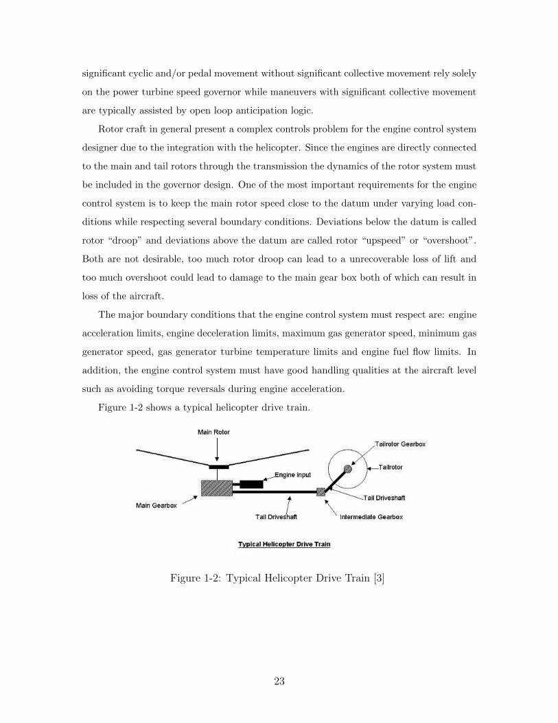
Figure 1-2 shows a typical helicopter drive train.
Figure 1-2: Typical Helicopter Drive Train [3]
23
1.2 Scope
The purpose of this research is to replace the baseline controller [1] with an LPV controller
while respecting the boundary conditions stated in section 1.1. The engine model is based
from the paper written by Mark G. Ballin of the NASA Ames Research Center [1]. Since,
a rotor model is not specifically presented in the paper by Ballin the rotor model inertia is
taken from the thesis of William Pfiel [6]. This research does not require a perfect match
of engine performance as compared to the actual T700 engine as the control system can be
applied to any plant satisfying the assumptions stated in section 1.1. This research does not
attempt to re-produce the collective anticipation logic and instead assumes that the load is
known to the control system.
24
Chapter 2
Engine Control System
The modeled engine is General Electric T700-GE-700 [1]. Two T700 engines are coupled
to the main gear box of a Sikorsky model UH-60A Black Hawk helicopter. Each engine is
capable of producing approximately 1800 shaft horsepower. The engine compressor consists
of 5 axial compressor stages and 1 centrifugal compressor stage. The compressor utilizes
variable geometry on the engine stators for improved stall protection at off design points.
Air flows from the exit of the centrifugal compressor through an annular combustor where
fuel is introduced and ignited. The hot air flows through the gas generator turbine which
extracts a portion of the energy to drive the compressor. The air exiting the gas generator
flows through the power turbine module which extracts the remaining energy driving the
shaft connected to the helicopter main gear box. The gas generator or core of the engine
spins independently from the power turbine module allowing the helicopter gear box speed
to be modulated to the same reference under varying load conditions.
25
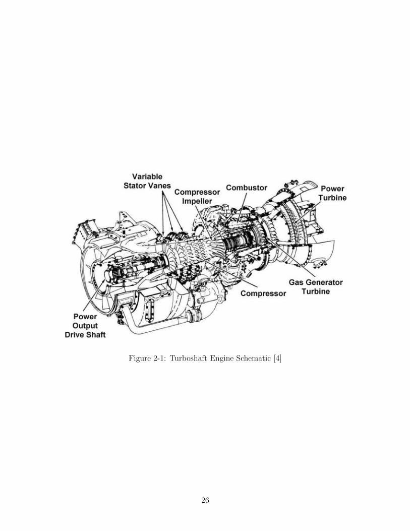
Figure 2-1: Turboshaft Engine Schematic [4]
26
Chapter 3
Engine Model
The T700 Engine model used as the plant for this research is based directly from the work
performed by Mark G. Ballin of the NASA Ames Research Center. The paper “A High
Fidelity Simulation of a Small Turboshaft Engine” [1] provides the equations to produce
a high fidelity non-linear simulation of the GE T700 engine. The equations are provided
in this thesis for reference and convenience however, this research is concentrated on the
development of an LPV controller provided in chapters 6 and 7. This engine is representative
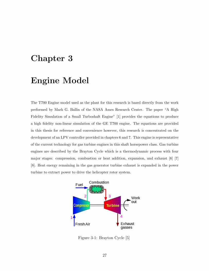
of the current technology for gas turbine engines in this shaft horsepower class. Gas turbine
engines are described by the Brayton Cycle which is a thermodynamic process with four
major stages: compression, combustion or heat addition, expansion, and exhaust [6] [7]
[8]. Heat energy remaining in the gas generator turbine exhaust is expanded in the power
turbine to extract power to drive the helicopter rotor system.
Figure 3-1: Brayton Cycle [5]
27
3.1 Engine Model Assumptions
The engine model assumes the following for the purposes of simplification:
1. The inlet losses are approximately equal to the static ambient conditions.
2. The engine heat sink is not included.
3. The variable geometry and bleed valves are assumed to be on schedule and are not
included in the control system.
4. Other engine model assumptions are provided in Ballin’s paper [1].
3.2 Engine Model Tools
The engine model is implemented in native Matlab�Simulink�to take advantage of the
Matlab�toolset including the LMI toolbox [2] which contains the tools used to create the
LPV controller in chapter 7.
3.3 Engine Model Architecture
The equations to build the engine model are given in fragments pictorially as they appear
in the Simulink�model or in equation form depending on which method provided the best
clarity in communicating the implementation. The complete set of Simulink�diagrams is
given in Appendix A. The variables in the equations refer to engine stations associated with
different sections of the engine gas path. The numbers start with zero at the beginning of
the engine and end with nine at the exhaust of the engine. The engine stations are shown
in Figure 3-2.
28
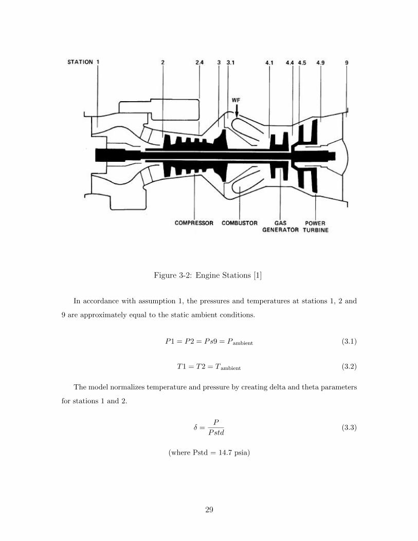
Figure 3-2: Engine Stations [1]
In accordance with assumption 1, the pressures and temperatures at stations 1, 2 and
9 are approximately equal to the static ambient conditions.
P1 = P2 = Ps9 = P ambient (3.1)
T1 = T2 = T ambient (3.2)
The model normalizes temperature and pressure by creating delta and theta parameters
for stations 1 and 2.
δ =P
Pstd(3.3)
(where Pstd = 14.7 psia)
29
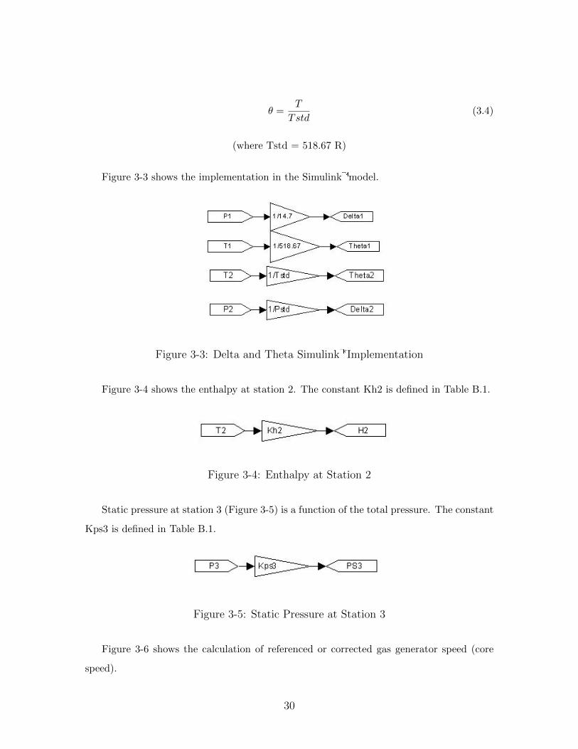
θ =T
Tstd(3.4)
(where Tstd = 518.67 R)
Figure 3-3 shows the implementation in the Simulink�model.
Figure 3-3: Delta and Theta Simulink�Implementation
Figure 3-4 shows the enthalpy at station 2. The constant Kh2 is defined in Table B.1.
Figure 3-4: Enthalpy at Station 2
Static pressure at station 3 (Figure 3-5) is a function of the total pressure. The constant
Kps3 is defined in Table B.1.
Figure 3-5: Static Pressure at Station 3
Figure 3-6 shows the calculation of referenced or corrected gas generator speed (core
speed).
30
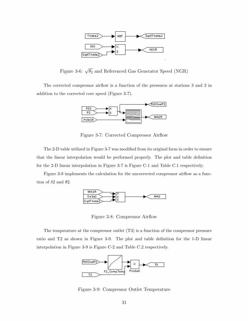
Figure 3-6:√θ2 and Referenced Gas Generator Speed (NGR)
The corrected compressor airflow is a function of the pressures at stations 3 and 2 in
addition to the corrected core speed (Figure 3-7).
Figure 3-7: Corrected Compressor Airflow
The 2-D table utilized in Figure 3-7 was modified from its original form in order to ensure
that the linear interpolation would be performed properly. The plot and table definition
for the 2-D linear interpolation in Figure 3-7 is Figure C-1 and Table C.1 respectively.
Figure 3-8 implements the calculation for the uncorrected compressor airflow as a func-
tion of δ2 and θ2.
Figure 3-8: Compressor Airflow
The temperature at the compressor outlet (T3) is a function of the compressor pressure
ratio and T2 as shown in Figure 3-9. The plot and table definition for the 1-D linear
interpolation in Figure 3-9 is Figure C-2 and Table C.2 respectively.
Figure 3-9: Compressor Outlet Temperature
31
The enthalpy at station 3 is defined by equation 3.5.
H3 = KH31 ∗ T3 +KH32 (3.5)
(where KH31 and KH32 are defined in Table B.1)
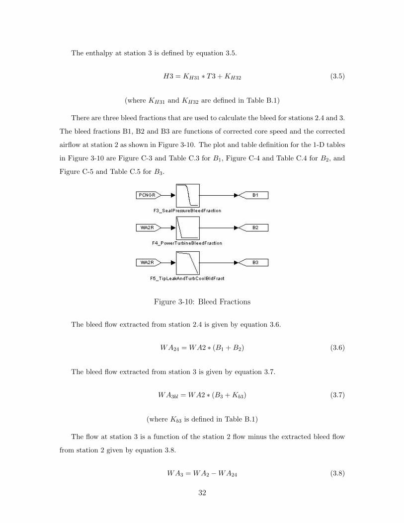
There are three bleed fractions that are used to calculate the bleed for stations 2.4 and 3.
The bleed fractions B1, B2 and B3 are functions of corrected core speed and the corrected
airflow at station 2 as shown in Figure 3-10. The plot and table definition for the 1-D tables
in Figure 3-10 are Figure C-3 and Table C.3 for B1, Figure C-4 and Table C.4 for B2, and
Figure C-5 and Table C.5 for B3.
Figure 3-10: Bleed Fractions
The bleed flow extracted from station 2.4 is given by equation 3.6.
WA24 = WA2 ∗ (B1 +B2) (3.6)
The bleed flow extracted from station 3 is given by equation 3.7.
WA3bl = WA2 ∗ (B3 +Kb3) (3.7)
(where Kb3 is defined in Table B.1)
The flow at station 3 is a function of the station 2 flow minus the extracted bleed flow
from station 2 given by equation 3.8.
WA3 = WA2 −WA24 (3.8)
32
The flow at station 3.1, combustor inlet, is a function of combustor inlet pressure and
temperature as well as the combustor outlet pressure given by equation 3.9.
WA31 =
√P3 ∗ (P3 − P41)
Kdbp ∗ T3(3.9)
(where Kdbp is defined in Table B.1)
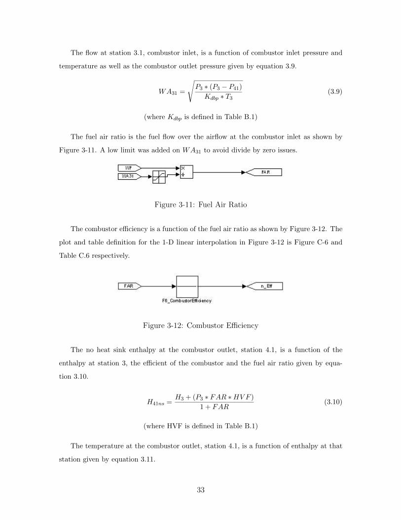
The fuel air ratio is the fuel flow over the airflow at the combustor inlet as shown by
Figure 3-11. A low limit was added on WA31 to avoid divide by zero issues.
Figure 3-11: Fuel Air Ratio
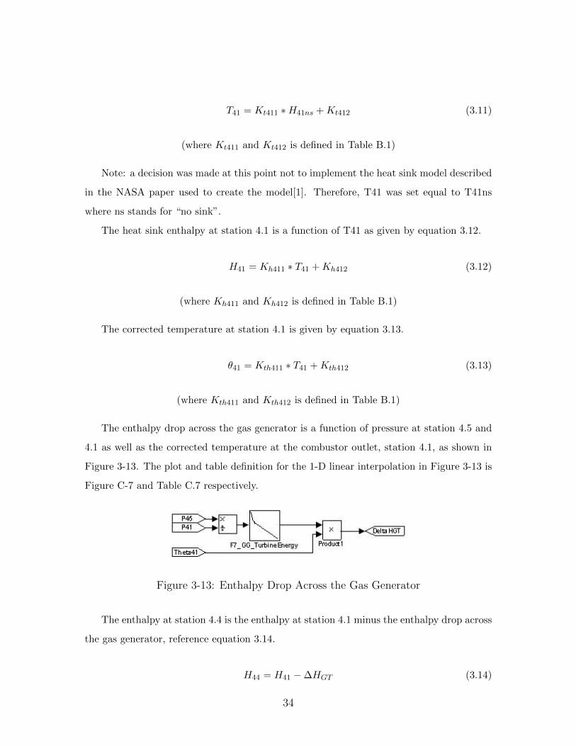
The combustor efficiency is a function of the fuel air ratio as shown by Figure 3-12. The
plot and table definition for the 1-D linear interpolation in Figure 3-12 is Figure C-6 and
Table C.6 respectively.
Figure 3-12: Combustor Efficiency
The no heat sink enthalpy at the combustor outlet, station 4.1, is a function of the
enthalpy at station 3, the efficient of the combustor and the fuel air ratio given by equa-
tion 3.10.
H41ns =H3 + (P3 ∗ FAR ∗HV F )
1 + FAR(3.10)
(where HVF is defined in Table B.1)
The temperature at the combustor outlet, station 4.1, is a function of enthalpy at that
station given by equation 3.11.
33
T41 = Kt411 ∗H41ns +Kt412 (3.11)
(where Kt411 and Kt412 is defined in Table B.1)
Note: a decision was made at this point not to implement the heat sink model described
in the NASA paper used to create the model[1]. Therefore, T41 was set equal to T41ns
where ns stands for “no sink”.
The heat sink enthalpy at station 4.1 is a function of T41 as given by equation 3.12.
H41 = Kh411 ∗ T41 +Kh412 (3.12)
(where Kh411 and Kh412 is defined in Table B.1)
The corrected temperature at station 4.1 is given by equation 3.13.
θ41 = Kth411 ∗ T41 +Kth412 (3.13)
(where Kth411 and Kth412 is defined in Table B.1)
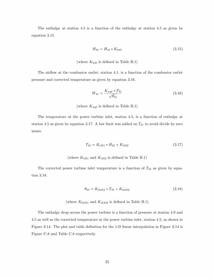
The enthalpy drop across the gas generator is a function of pressure at station 4.5 and
4.1 as well as the corrected temperature at the combustor outlet, station 4.1, as shown in
Figure 3-13. The plot and table definition for the 1-D linear interpolation in Figure 3-13 is
Figure C-7 and Table C.7 respectively.
Figure 3-13: Enthalpy Drop Across the Gas Generator
The enthalpy at station 4.4 is the enthalpy at station 4.1 minus the enthalpy drop across
the gas generator, reference equation 3.14.
H44 = H41 −∆HGT (3.14)
34
The enthalpy at station 4.5 is a function of the enthalpy at station 4.5 as given be
equation 3.15.
H45 = H44 ∗Kh45 (3.15)
(where Kh45 is defined in Table B.1)
The airflow at the combustor outlet, station 4.1, is a function of the combustor outlet
pressure and corrected temperature as given by equation 3.16.
W41 =Kwgt ∗ P41√
θ41(3.16)
(where Kwgt is defined in Table B.1)
The temperature at the power turbine inlet, station 4.5, is a function of enthalpy at
station 4.5 as given by equation 3.17. A low limit was added on T41 to avoid divide by zero
issues.
T45 = Kt451 ∗H45 +Kt452 (3.17)
(where Kt451 and Kt452 is defined in Table B.1)
The corrected power turbine inlet temperature is a function of T45 as given by equa-
tion 3.18.
θ45 = Kth451 ∗ T45 +Kth452 (3.18)
(where Kth451 and Kth452 is defined in Table B.1)
The enthalpy drop across the power turbine is a function of pressure at station 4.9 and
4.5 as well as the corrected temperature at the power turbine inlet, station 4.5, as shown in
Figure 3-14. The plot and table definition for the 1-D linear interpolation in Figure 3-14 is
Figure C-8 and Table C.8 respectively.
35
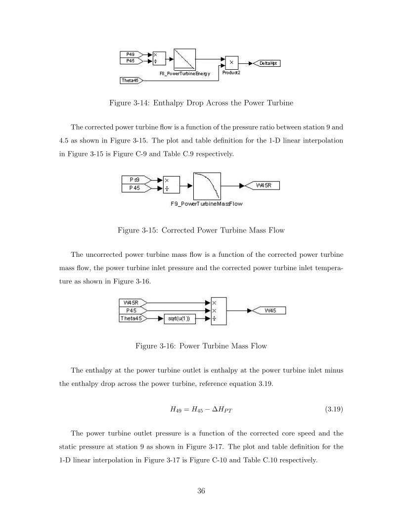
Figure 3-14: Enthalpy Drop Across the Power Turbine
The corrected power turbine flow is a function of the pressure ratio between station 9 and
4.5 as shown in Figure 3-15. The plot and table definition for the 1-D linear interpolation
in Figure 3-15 is Figure C-9 and Table C.9 respectively.
Figure 3-15: Corrected Power Turbine Mass Flow
The uncorrected power turbine mass flow is a function of the corrected power turbine
mass flow, the power turbine inlet pressure and the corrected power turbine inlet tempera-
ture as shown in Figure 3-16.
Figure 3-16: Power Turbine Mass Flow
The enthalpy at the power turbine outlet is enthalpy at the power turbine inlet minus
the enthalpy drop across the power turbine, reference equation 3.19.
H49 = H45 −∆HPT (3.19)
The power turbine outlet pressure is a function of the corrected core speed and the
static pressure at station 9 as shown in Figure 3-17. The plot and table definition for the
1-D linear interpolation in Figure 3-17 is Figure C-10 and Table C.10 respectively.
36
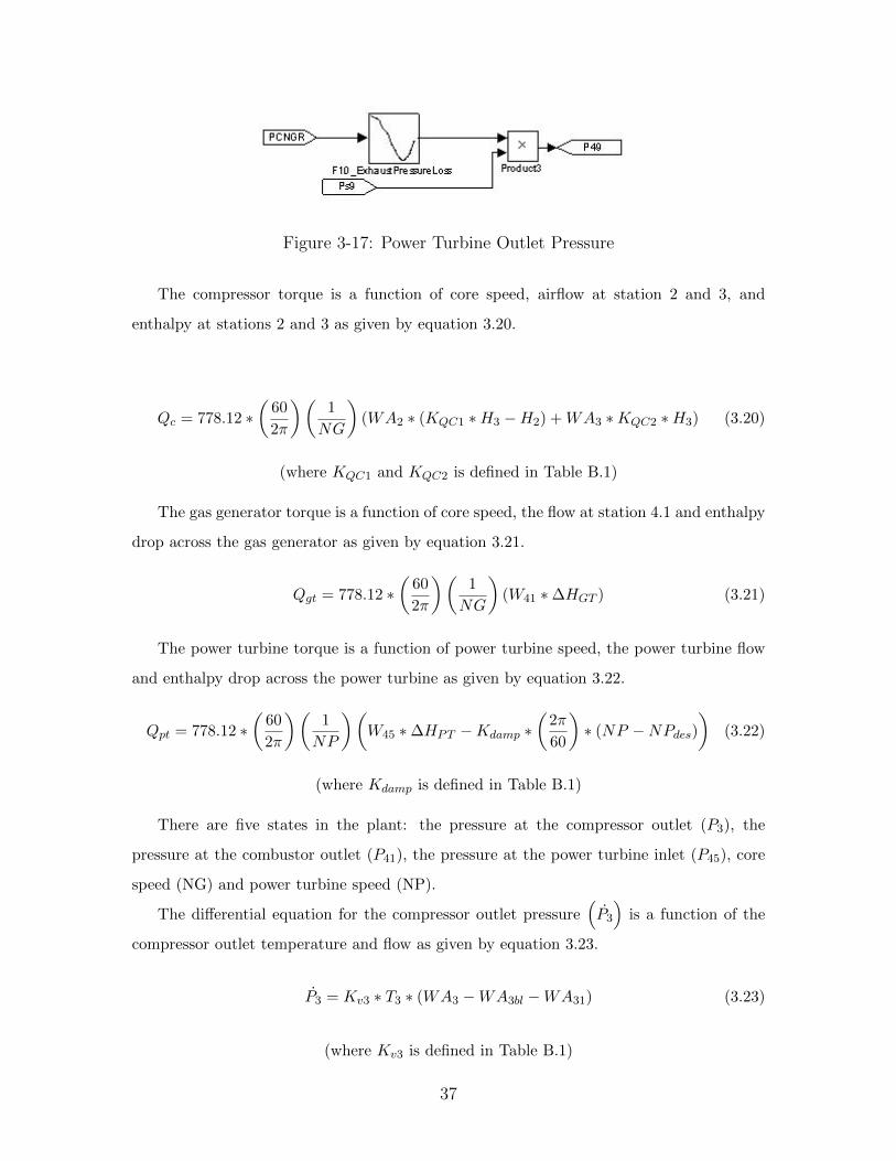
Figure 3-17: Power Turbine Outlet Pressure
The compressor torque is a function of core speed, airflow at station 2 and 3, and
enthalpy at stations 2 and 3 as given by equation 3.20.
Qc = 778.12 ∗(
60
2π
)(1
NG
)(WA2 ∗ (KQC1 ∗H3 −H2) +WA3 ∗KQC2 ∗H3) (3.20)
(where KQC1 and KQC2 is defined in Table B.1)
The gas generator torque is a function of core speed, the flow at station 4.1 and enthalpy
drop across the gas generator as given by equation 3.21.
Qgt = 778.12 ∗(
60
2π
)(1
NG
)(W41 ∗∆HGT ) (3.21)
The power turbine torque is a function of power turbine speed, the power turbine flow
and enthalpy drop across the power turbine as given by equation 3.22.
Qpt = 778.12 ∗(
60
2π
)(1
NP
)(W45 ∗∆HPT −Kdamp ∗
(2π
60
)∗ (NP −NPdes)
)(3.22)
(where Kdamp is defined in Table B.1)
There are five states in the plant: the pressure at the compressor outlet (P3), the
pressure at the combustor outlet (P41), the pressure at the power turbine inlet (P45), core
speed (NG) and power turbine speed (NP).
The differential equation for the compressor outlet pressure(P3
)is a function of the
compressor outlet temperature and flow as given by equation 3.23.
P3 = Kv3 ∗ T3 ∗ (WA3 −WA3bl −WA31) (3.23)
(where Kv3 is defined in Table B.1)
37
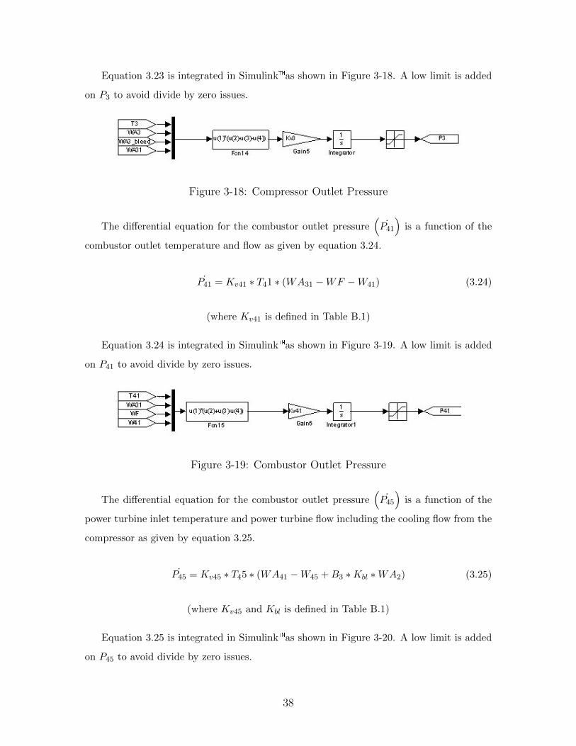
Equation 3.23 is integrated in Simulink�as shown in Figure 3-18. A low limit is added
on P3 to avoid divide by zero issues.
Figure 3-18: Compressor Outlet Pressure
The differential equation for the combustor outlet pressure(
˙P41
)is a function of the
combustor outlet temperature and flow as given by equation 3.24.
˙P41 = Kv41 ∗ T41 ∗ (WA31 −WF −W41) (3.24)
(where Kv41 is defined in Table B.1)
Equation 3.24 is integrated in Simulink�as shown in Figure 3-19. A low limit is added
on P41 to avoid divide by zero issues.
Figure 3-19: Combustor Outlet Pressure
The differential equation for the combustor outlet pressure(
˙P45
)is a function of the
power turbine inlet temperature and power turbine flow including the cooling flow from the
compressor as given by equation 3.25.
˙P45 = Kv45 ∗ T45 ∗ (WA41 −W45 +B3 ∗Kbl ∗WA2) (3.25)
(where Kv45 and Kbl is defined in Table B.1)
Equation 3.25 is integrated in Simulink�as shown in Figure 3-20. A low limit is added
on P45 to avoid divide by zero issues.
38
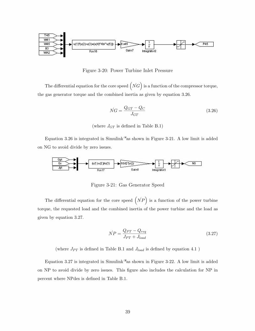
Figure 3-20: Power Turbine Inlet Pressure
The differential equation for the core speed(
˙NG)
is a function of the compressor torque,
the gas generator torque and the combined inertia as given by equation 3.26.
˙NG =QGT −QC
JGT(3.26)
(where JGT is defined in Table B.1)
Equation 3.26 is integrated in Simulink�as shown in Figure 3-21. A low limit is added
on NG to avoid divide by zero issues.
Figure 3-21: Gas Generator Speed
The differential equation for the core speed(
˙NP)
is a function of the power turbine
torque, the requested load and the combined inertia of the power turbine and the load as
given by equation 3.27.
˙NP =QPT −Qreq
JPT + Jload(3.27)
(where JPT is defined in Table B.1 and Jload is defined by equation 4.1 )
Equation 3.27 is integrated in Simulink�as shown in Figure 3-22. A low limit is added
on NP to avoid divide by zero issues. This figure also includes the calculation for NP in
percent where NPdes is defined in Table B.1.
39
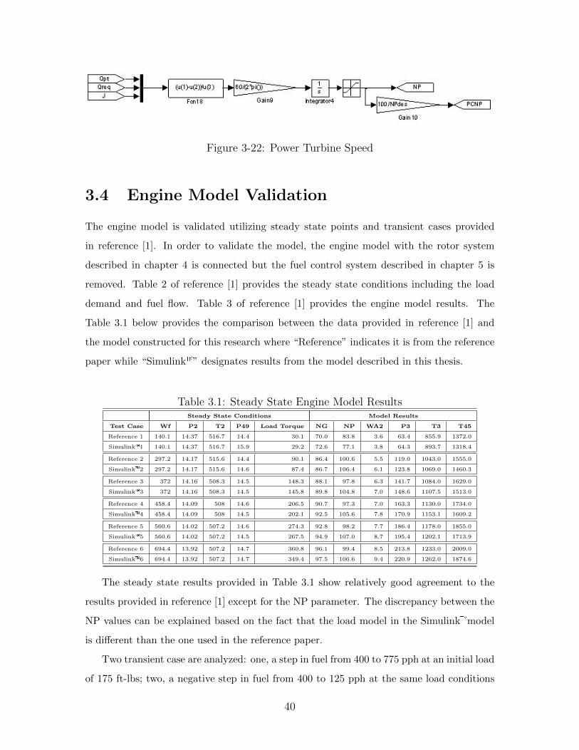
Figure 3-22: Power Turbine Speed
3.4 Engine Model Validation
The engine model is validated utilizing steady state points and transient cases provided
in reference [1]. In order to validate the model, the engine model with the rotor system
described in chapter 4 is connected but the fuel control system described in chapter 5 is
removed. Table 2 of reference [1] provides the steady state conditions including the load
demand and fuel flow. Table 3 of reference [1] provides the engine model results. The
Table 3.1 below provides the comparison between the data provided in reference [1] and
the model constructed for this research where “Reference” indicates it is from the reference
paper while “Simulink�” designates results from the model described in this thesis.
Table 3.1: Steady State Engine Model ResultsSteady State Conditions Model Results
Test Case Wf P2 T2 P49 Load Torque NG NP WA2 P3 T3 T45
Reference 1 140.1 14.37 516.7 14.4 30.1 70.0 83.8 3.6 63.4 855.9 1372.0
Simulink�1 140.1 14.37 516.7 15.9 29.2 72.6 77.1 3.8 64.3 893.7 1318.4
Reference 2 297.2 14.17 515.6 14.4 90.1 86.4 100.6 5.5 119.0 1043.0 1555.0
Simulink�2 297.2 14.17 515.6 14.6 87.4 86.7 106.4 6.1 123.8 1069.0 1460.3
Reference 3 372 14.16 508.3 14.5 148.3 88.1 97.8 6.3 141.7 1084.0 1629.0
Simulink�3 372 14.16 508.3 14.5 145.8 89.8 104.8 7.0 148.6 1107.5 1513.0
Reference 4 458.4 14.09 508 14.6 206.5 90.7 97.3 7.0 163.3 1130.0 1734.0
Simulink�4 458.4 14.09 508 14.5 202.1 92.5 105.6 7.8 170.9 1153.1 1609.2
Reference 5 560.6 14.02 507.2 14.6 274.3 92.8 98.2 7.7 186.4 1178.0 1855.0
Simulink�5 560.6 14.02 507.2 14.5 267.5 94.9 107.0 8.7 195.4 1202.1 1713.9
Reference 6 694.4 13.92 507.2 14.7 360.8 96.1 99.4 8.5 213.8 1233.0 2009.0
Simulink�6 694.4 13.92 507.2 14.7 349.4 97.5 106.6 9.4 220.9 1262.0 1874.6
The steady state results provided in Table 3.1 show relatively good agreement to the
results provided in reference [1] except for the NP parameter. The discrepancy between the
NP values can be explained based on the fact that the load model in the Simulink�model
is different than the one used in the reference paper.
Two transient case are analyzed: one, a step in fuel from 400 to 775 pph at an initial load
of 175 ft-lbs; two, a negative step in fuel from 400 to 125 pph at the same load conditions
40
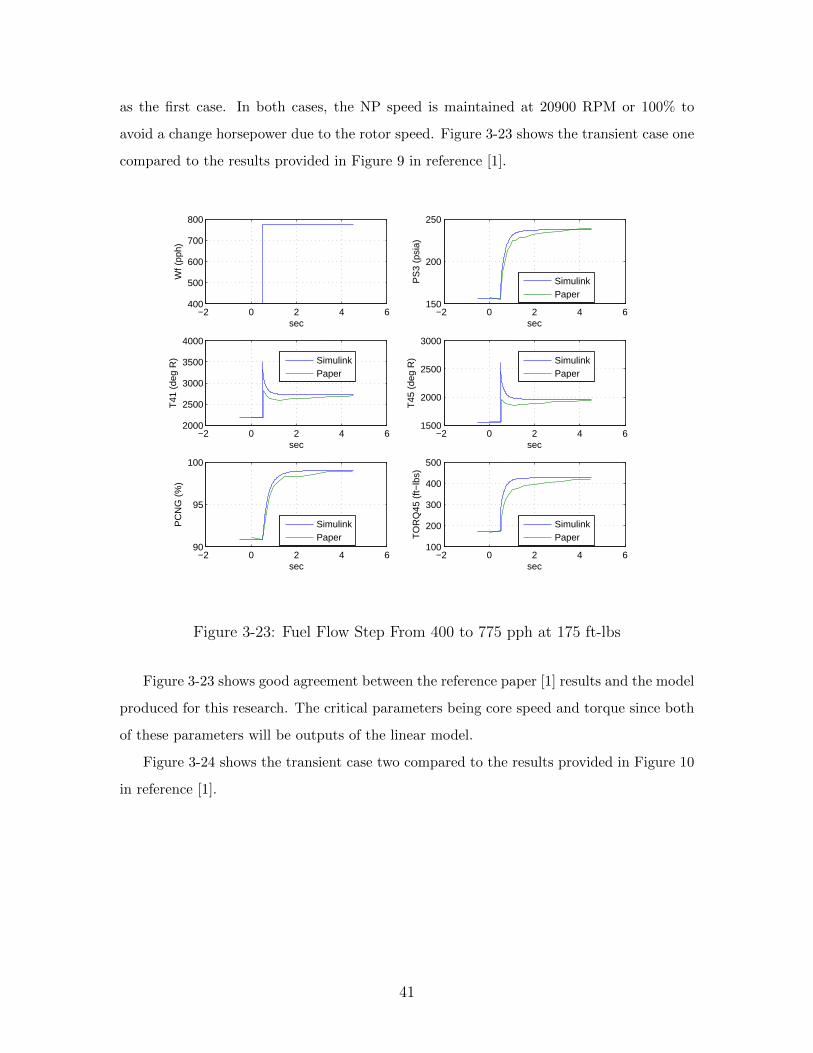
as the first case. In both cases, the NP speed is maintained at 20900 RPM or 100% to
avoid a change horsepower due to the rotor speed. Figure 3-23 shows the transient case one
compared to the results provided in Figure 9 in reference [1].
−2 0 2 4 6400
500
600
700
800
sec
Wf (
pph)
−2 0 2 4 6150
200
250
sec
PS
3 (p
sia)
SimulinkPaper
−2 0 2 4 62000
2500
3000
3500
4000
sec
T41
(de
g R
)
SimulinkPaper
−2 0 2 4 61500
2000
2500
3000
sec
T45
(de
g R
)
SimulinkPaper
−2 0 2 4 690
95
100
sec
PC
NG
(%
)
SimulinkPaper
−2 0 2 4 6100
200
300
400
500
sec
TO
RQ
45 (
ft−lb
s)
SimulinkPaper
Figure 3-23: Fuel Flow Step From 400 to 775 pph at 175 ft-lbs
Figure 3-23 shows good agreement between the reference paper [1] results and the model
produced for this research. The critical parameters being core speed and torque since both
of these parameters will be outputs of the linear model.
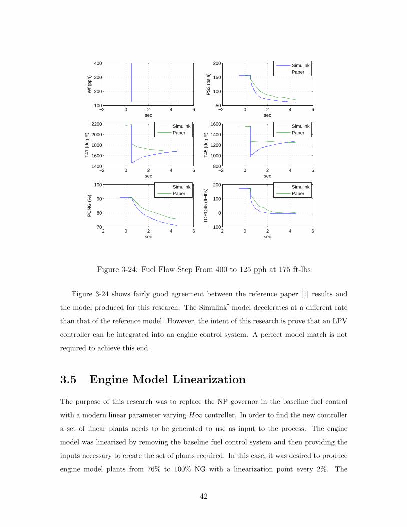
Figure 3-24 shows the transient case two compared to the results provided in Figure 10
in reference [1].
41
−2 0 2 4 6100
200
300
400
sec
Wf (
pph)
−2 0 2 4 650
100
150
200
sec
PS
3 (p
sia)
−2 0 2 4 61400
1600
1800
2000
2200
sec
T41
(de
g R
)
−2 0 2 4 6800
1000
1200
1400
1600
sec
T45
(de
g R
)
−2 0 2 4 670
80
90
100
sec
PC
NG
(%
)
−2 0 2 4 6−100
0
100
200
sec
TO
RQ
45 (
ft−lb
s)
SimulinkPaper
SimulinkPaper
SimulinkPaper
SimulinkPaper
SimulinkPaper
Figure 3-24: Fuel Flow Step From 400 to 125 pph at 175 ft-lbs
Figure 3-24 shows fairly good agreement between the reference paper [1] results and
the model produced for this research. The Simulink�model decelerates at a different rate
than that of the reference model. However, the intent of this research is prove that an LPV
controller can be integrated into an engine control system. A perfect model match is not
required to achieve this end.
3.5 Engine Model Linearization
The purpose of this research was to replace the NP governor in the baseline fuel control
with a modern linear parameter varying H∞ controller. In order to find the new controller
a set of linear plants needs to be generated to use as input to the process. The engine
model was linearized by removing the baseline fuel control system and then providing the
inputs necessary to create the set of plants required. In this case, it was desired to produce
engine model plants from 76% to 100% NG with a linearization point every 2%. The
42
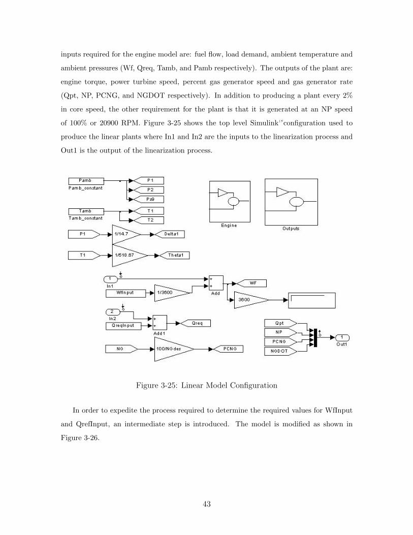
inputs required for the engine model are: fuel flow, load demand, ambient temperature and
ambient pressures (Wf, Qreq, Tamb, and Pamb respectively). The outputs of the plant are:
engine torque, power turbine speed, percent gas generator speed and gas generator rate
(Qpt, NP, PCNG, and NGDOT respectively). In addition to producing a plant every 2%
in core speed, the other requirement for the plant is that it is generated at an NP speed
of 100% or 20900 RPM. Figure 3-25 shows the top level Simulink�configuration used to
produce the linear plants where In1 and In2 are the inputs to the linearization process and
Out1 is the output of the linearization process.
Figure 3-25: Linear Model Configuration
In order to expedite the process required to determine the required values for WfInput
and QrefInput, an intermediate step is introduced. The model is modified as shown in
Figure 3-26.
43
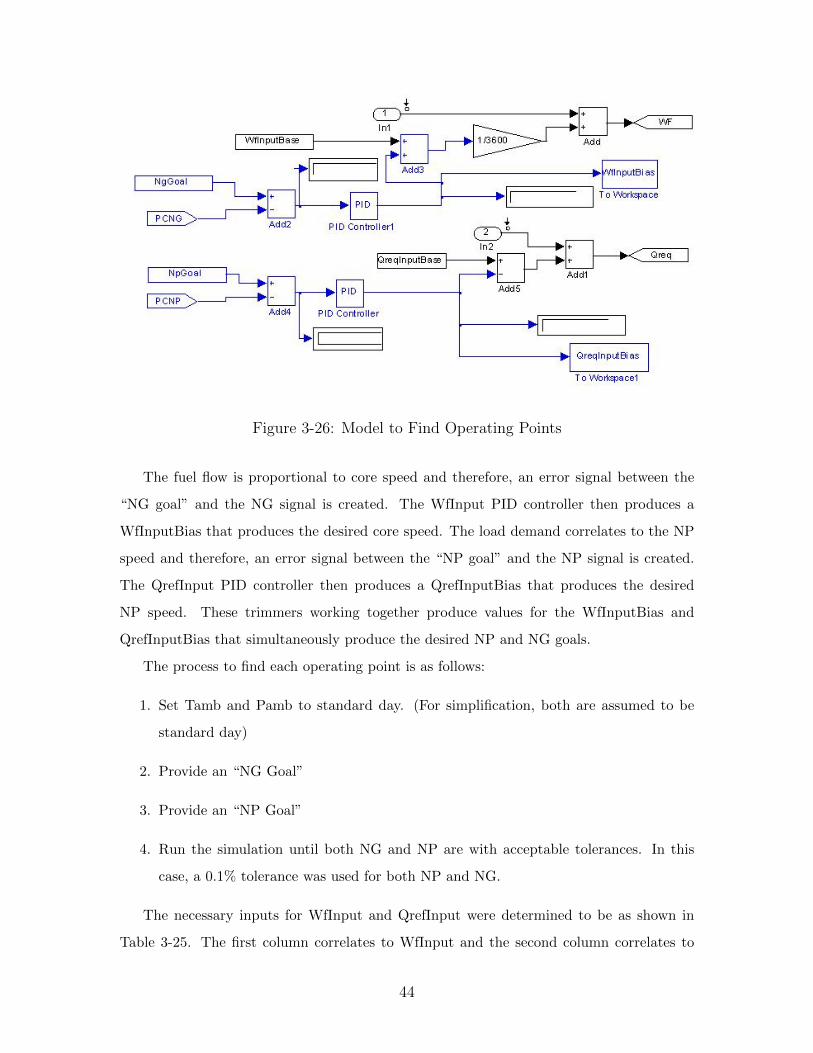
Figure 3-26: Model to Find Operating Points
The fuel flow is proportional to core speed and therefore, an error signal between the
“NG goal” and the NG signal is created. The WfInput PID controller then produces a
WfInputBias that produces the desired core speed. The load demand correlates to the NP
speed and therefore, an error signal between the “NP goal” and the NP signal is created.
The QrefInput PID controller then produces a QrefInputBias that produces the desired
NP speed. These trimmers working together produce values for the WfInputBias and
QrefInputBias that simultaneously produce the desired NP and NG goals.
The process to find each operating point is as follows:
1. Set Tamb and Pamb to standard day. (For simplification, both are assumed to be
standard day)
2. Provide an “NG Goal”
3. Provide an “NP Goal”
4. Run the simulation until both NG and NP are with acceptable tolerances. In this
case, a 0.1% tolerance was used for both NP and NG.
The necessary inputs for WfInput and QrefInput were determined to be as shown in
Table 3-25. The first column correlates to WfInput and the second column correlates to
44
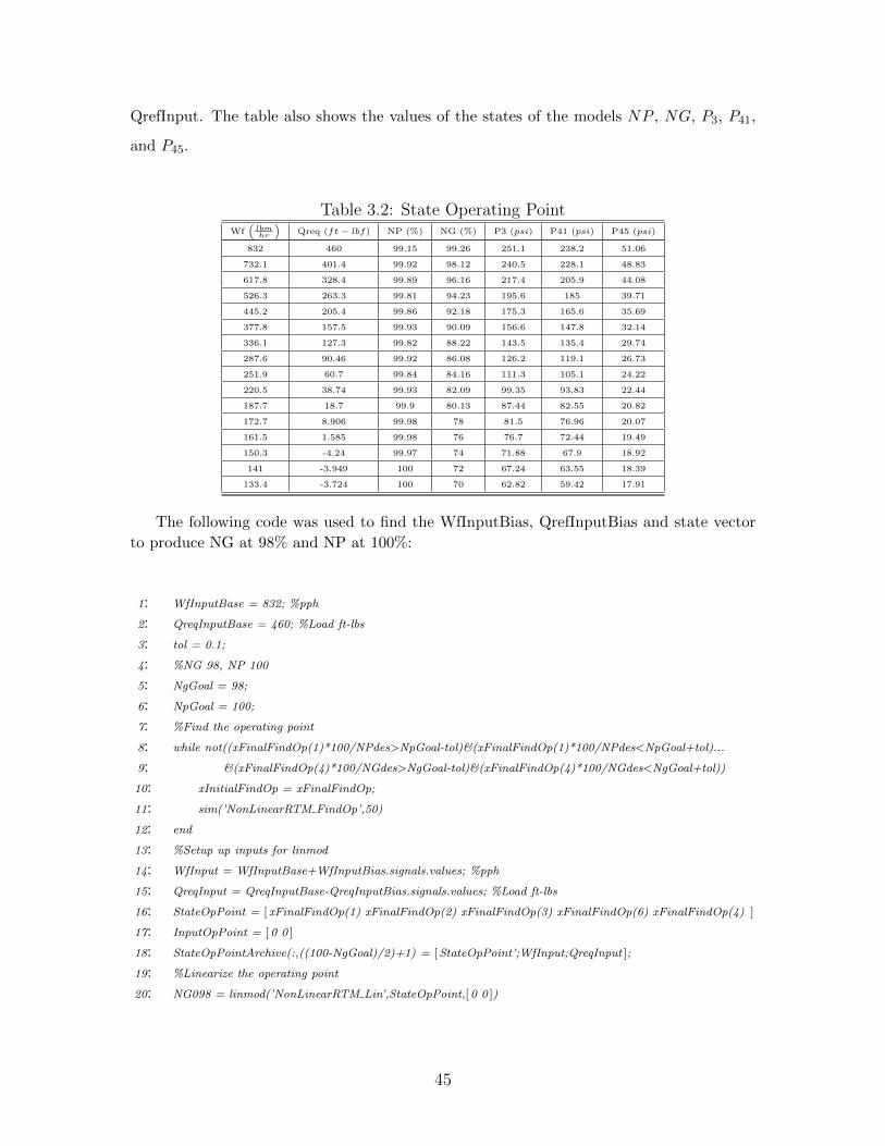
QrefInput. The table also shows the values of the states of the models NP , NG, P3, P41,
and P45.
Table 3.2: State Operating PointWf
(lbmhr
)Qreq (ft− lbf) NP (%) NG (%) P3 (psi) P41 (psi) P45 (psi)
832 460 99.15 99.26 251.1 238.2 51.06
732.1 401.4 99.92 98.12 240.5 228.1 48.83
617.8 328.4 99.89 96.16 217.4 205.9 44.08
526.3 263.3 99.81 94.23 195.6 185 39.71
445.2 205.4 99.86 92.18 175.3 165.6 35.69
377.8 157.5 99.93 90.09 156.6 147.8 32.14
336.1 127.3 99.82 88.22 143.5 135.4 29.74
287.6 90.46 99.92 86.08 126.2 119.1 26.73
251.9 60.7 99.84 84.16 111.3 105.1 24.22
220.5 38.74 99.93 82.09 99.35 93.83 22.44
187.7 18.7 99.9 80.13 87.44 82.55 20.82
172.7 8.906 99.98 78 81.5 76.96 20.07
161.5 1.585 99.98 76 76.7 72.44 19.49
150.3 -4.24 99.97 74 71.88 67.9 18.92
141 -3.949 100 72 67.24 63.55 18.39
133.4 -3.724 100 70 62.82 59.42 17.91
The following code was used to find the WfInputBias, QrefInputBias and state vector
to produce NG at 98% and NP at 100%:
1: WfInputBase = 832; %pph
2: QreqInputBase = 460; %Load ft-lbs
3: tol = 0.1;
4: %NG 98, NP 100
5: NgGoal = 98;
6: NpGoal = 100;
7: %Find the operating point
8: while not((xFinalFindOp(1)*100/NPdes>NpGoal-tol)&(xFinalFindOp(1)*100/NPdes<NpGoal+tol)...
9: &(xFinalFindOp(4)*100/NGdes>NgGoal-tol)&(xFinalFindOp(4)*100/NGdes<NgGoal+tol))
10: xInitialFindOp = xFinalFindOp;
11: sim(’NonLinearRTM FindOp’,50)
12: end
13: %Setup up inputs for linmod
14: WfInput = WfInputBase+WfInputBias.signals.values; %pph
15: QreqInput = QreqInputBase-QreqInputBias.signals.values; %Load ft-lbs
16: StateOpPoint = [ xFinalFindOp(1) xFinalFindOp(2) xFinalFindOp(3) xFinalFindOp(6) xFinalFindOp(4) ]
17: InputOpPoint = [0 0 ]
18: StateOpPointArchive(:,((100-NgGoal)/2)+1) = [StateOpPoint’;WfInput;QreqInput ];
19: %Linearize the operating point
20: NG098 = linmod(’NonLinearRTM Lin’,StateOpPoint,[0 0 ])
45
The complete m-file used to create all of the linearized plants can be found in ap-
pendix G.2.
The result from the code in appendix G.2 is a set of plants between 76% and 100%
NG with points every 2% NG. The state space matrices and eigenvalues for each of the
plants is in appendix H.1. At this point, the eigenvalues are reviewed to determine if the
plants are stable or unstable. In addition, the eigenvalues obtained are compared against
the eigenvalues from Ballin’s work the baseline paper “A High Fidelity Simulation of a
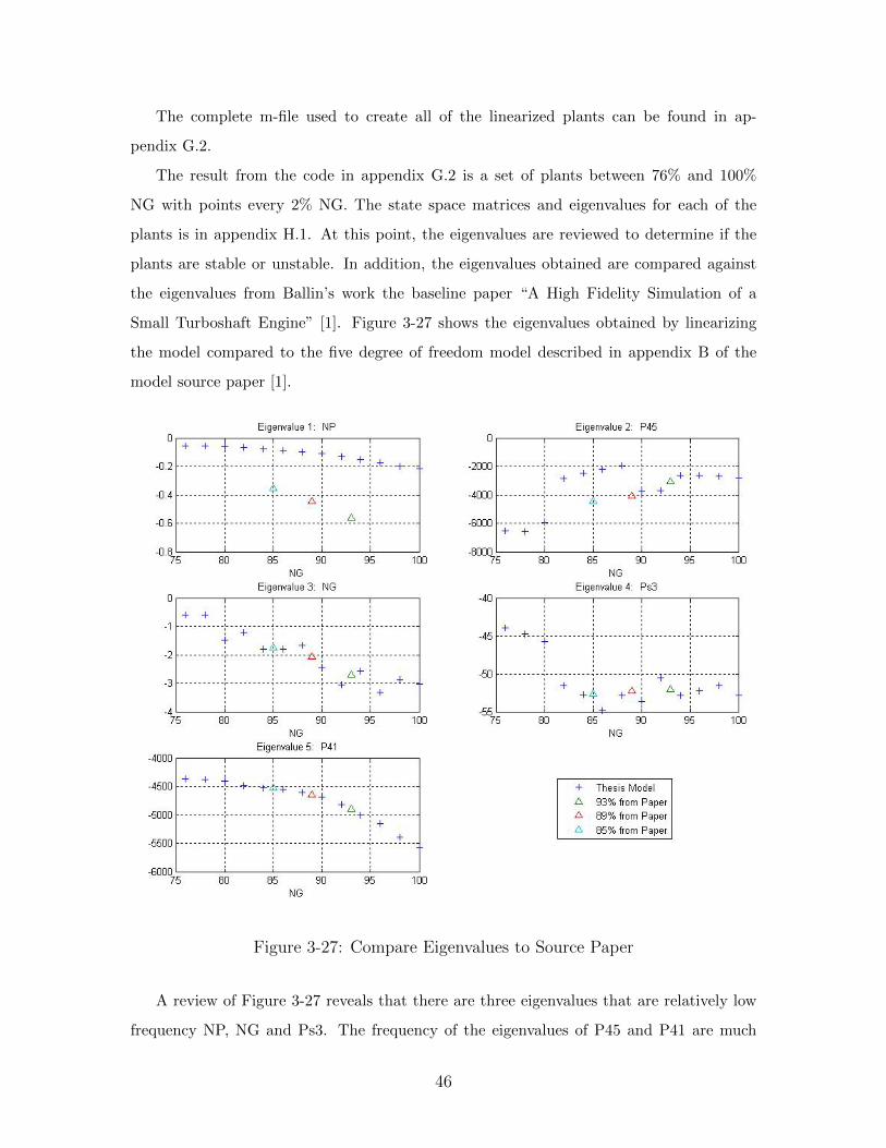
Small Turboshaft Engine” [1]. Figure 3-27 shows the eigenvalues obtained by linearizing
the model compared to the five degree of freedom model described in appendix B of the
model source paper [1].
Figure 3-27: Compare Eigenvalues to Source Paper
A review of Figure 3-27 reveals that there are three eigenvalues that are relatively low
frequency NP, NG and Ps3. The frequency of the eigenvalues of P45 and P41 are much
46

higher than bandwidth of the baseline controller and the LPV controller. Therefore, if
desired the model can be simplified by eliminating the three highest frequency eigenvalues.
47
Chapter 4
Load Model
The load demand model used for this research is based on the T700 engine model capabil-
ities. Two engines running at the maximum core speed producing the torque required to
maintain the rotor speed at 100% is defined as the 100% collective point. The zero percent
collective point is defined as zero shaft horsepower required. The curve between zero and
maximum load required follow a third order polynomial as given by equation 4.2. The load
model described in this chapter is compatible with the single pole rotor model described in
reference [1] that the engine model and baseline engine controller is derived from.
4.1 Load Model Assumptions
The following assumptions are applied to the construction of the load model:
1. The rotor can be represented the lumped inertia of the entire rotor system including
the main gear box. In practice, helicopter rotor models are normally much more
complex requiring attenuation for the main and tail rotor natural frequencies.
2. The collective to load application follows is a 3rd order polynomial.
3. The collective actuator response can be modeled by a simple lag.
4. The load remains constant across all airspeeds.
48
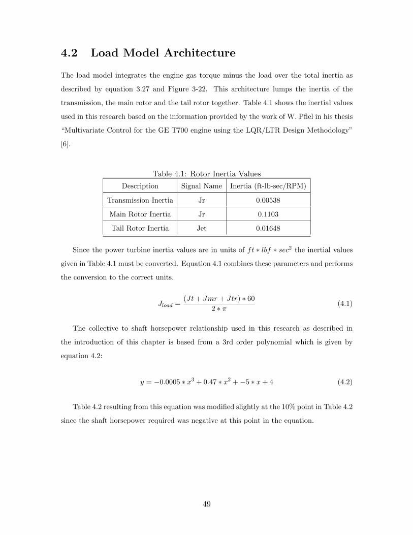
4.2 Load Model Architecture
The load model integrates the engine gas torque minus the load over the total inertia as
described by equation 3.27 and Figure 3-22. This architecture lumps the inertia of the
transmission, the main rotor and the tail rotor together. Table 4.1 shows the inertial values
used in this research based on the information provided by the work of W. Pfiel in his thesis
“Multivariate Control for the GE T700 engine using the LQR/LTR Design Methodology”
[6].
Table 4.1: Rotor Inertia Values
Description Signal Name Inertia (ft-lb-sec/RPM)
Transmission Inertia Jr 0.00538
Main Rotor Inertia Jr 0.1103
Tail Rotor Inertia Jet 0.01648
Since the power turbine inertia values are in units of ft ∗ lbf ∗ sec2 the inertial values
given in Table 4.1 must be converted. Equation 4.1 combines these parameters and performs
the conversion to the correct units.
Jload =(Jt+ Jmr + Jtr) ∗ 60
2 ∗ π(4.1)
The collective to shaft horsepower relationship used in this research as described in
the introduction of this chapter is based from a 3rd order polynomial which is given by
equation 4.2:
y = −0.0005 ∗ x3 + 0.47 ∗ x2 +−5 ∗ x+ 4 (4.2)
Table 4.2 resulting from this equation was modified slightly at the 10% point in Table 4.2
since the shaft horsepower required was negative at this point in the equation.
49
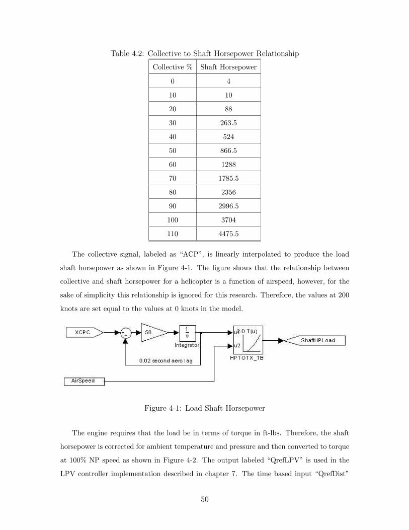
Table 4.2: Collective to Shaft Horsepower Relationship
Collective % Shaft Horsepower
0 4
10 10
20 88
30 263.5
40 524
50 866.5
60 1288
70 1785.5
80 2356
90 2996.5
100 3704
110 4475.5
The collective signal, labeled as “ACP”, is linearly interpolated to produce the load
shaft horsepower as shown in Figure 4-1. The figure shows that the relationship between
collective and shaft horsepower for a helicopter is a function of airspeed, however, for the
sake of simplicity this relationship is ignored for this research. Therefore, the values at 200
knots are set equal to the values at 0 knots in the model.
Figure 4-1: Load Shaft Horsepower
The engine requires that the load be in terms of torque in ft-lbs. Therefore, the shaft
horsepower is corrected for ambient temperature and pressure and then converted to torque
at 100% NP speed as shown in Figure 4-2. The output labeled “QrefLPV” is used in the
LPV controller implementation described in chapter 7. The time based input “QrefDist”
50
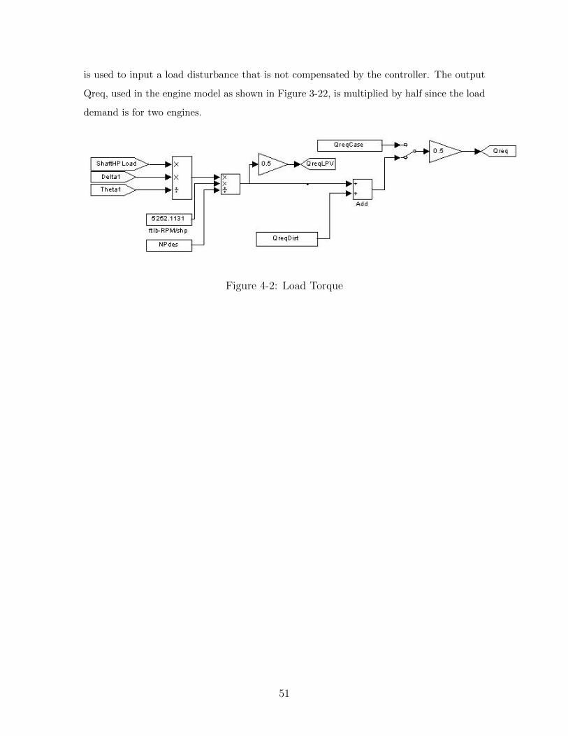
is used to input a load disturbance that is not compensated by the controller. The output
Qreq, used in the engine model as shown in Figure 3-22, is multiplied by half since the load
demand is for two engines.
Figure 4-2: Load Torque
51
Chapter 5
Engine Baseline Control System
Model
The T700 fuel control system model used as the baseline for this research was taken from
the paper written by Mark G. Ballin of the NASA Ames Research Center. The paper
“A High Fidelity Simulation of a Small Turbofan Engine” [1] provides the equations to
produce a high fidelity non-linear simulation of the GE T700 engine. The equations are
provided in this chapter for reference and convenience. The fuel control system provided
as the baseline is legacy technology involving a hydro-mechanical fuel unit (HMU) with
a digital trimming system. Current fuel control systems are based on a Full Authority
Digital Electronic Controller or FADEC which replace the most of the legacy controls with
electronic equivalents within the FADEC. However, the control system is still in use today
on several helicopter applications. In addition, the equations used to design HMU systems
are transferrable to a FADEC/FMU (fuel metering unit) system.
The control system on the T700 engine controls the fuel flow, the variable geometry, and
the operability bleed flow. The equations presented assume that the variable geometry and
operability bleed flow are controlled as scheduled. The equations for the plant make this
assumption as well. Therefore, the control system in this analysis considers only control of
the fuel flow into the engine. There are several boundary conditions that are considered
when designing a fuel control:
1. The following items are in order of decreasing importance:
52
(a) The core speed deceleration rate shall be greater than or equal to a minimum
scheduled reference.
(b) The core speed acceleration rate shall be less than or equal to a maximum
schedule reference.
(c) The core speed shall be greater than or equal to a minimum scheduled reference.
(d) The maximum fuel flow shall be less than or equal to a maximum scheduled
reference.
(e) The core speed shall be less than or equal to a maximum scheduled reference.
(f) The power available shall be less than or equal to the schedule set by the power
available spindle.
(g) The power turbine reference shall be kept at 100% or 20900 RPM.
2. It should be noted that the core speed acceleration is governed only byWf
Ps3and not
by ˙NG.
The purpose of this research is to determine if a modern linear parameter varying control
system can take the place of the baseline controller in controlling the NP speed.
5.1 Baseline Controller Assumptions
The following assumptions are applied to the construction of the baseline engine fuel control
model:
1. The model employs the following simplifications:
(a) The variable geometry and bleed valves are assumed to be on schedule and are
not included in the modeled control system.
(b) The T45 governor reference is set at a value such that it will not come into
regulation as this governor is not part of the primary analysis.
(c) The fuel flow actuator is modeled as a simple lag.
(d) The torque of the two engines is identical. Therefore, the load share governor
is ignored as it is not part of the primary analysis.
53
5.2 Baseline Controller Tools
The engine control system model is implemented in native Matlab�Simulink�since the
engine model and the LPV controller were also implemented in Simulink�facilitating the
back to back comparison.
5.3 Baseline Controller Architecture
The equations to build the baseline fuel control system model are given pictorially in frag-
ments as they appear in the Simulink�model. The complete set of Simulink�diagrams is
given in Appendix D. The variable names used in the diagrams and equations below are
defined in the Nomenclature section starting on page 14.
There are two inputs into the plant that determine where the engine will operate. The
fuel flow is provided by the fuel control system and the requested load is derived from the
rotor system model which is discussed in chapter 4.
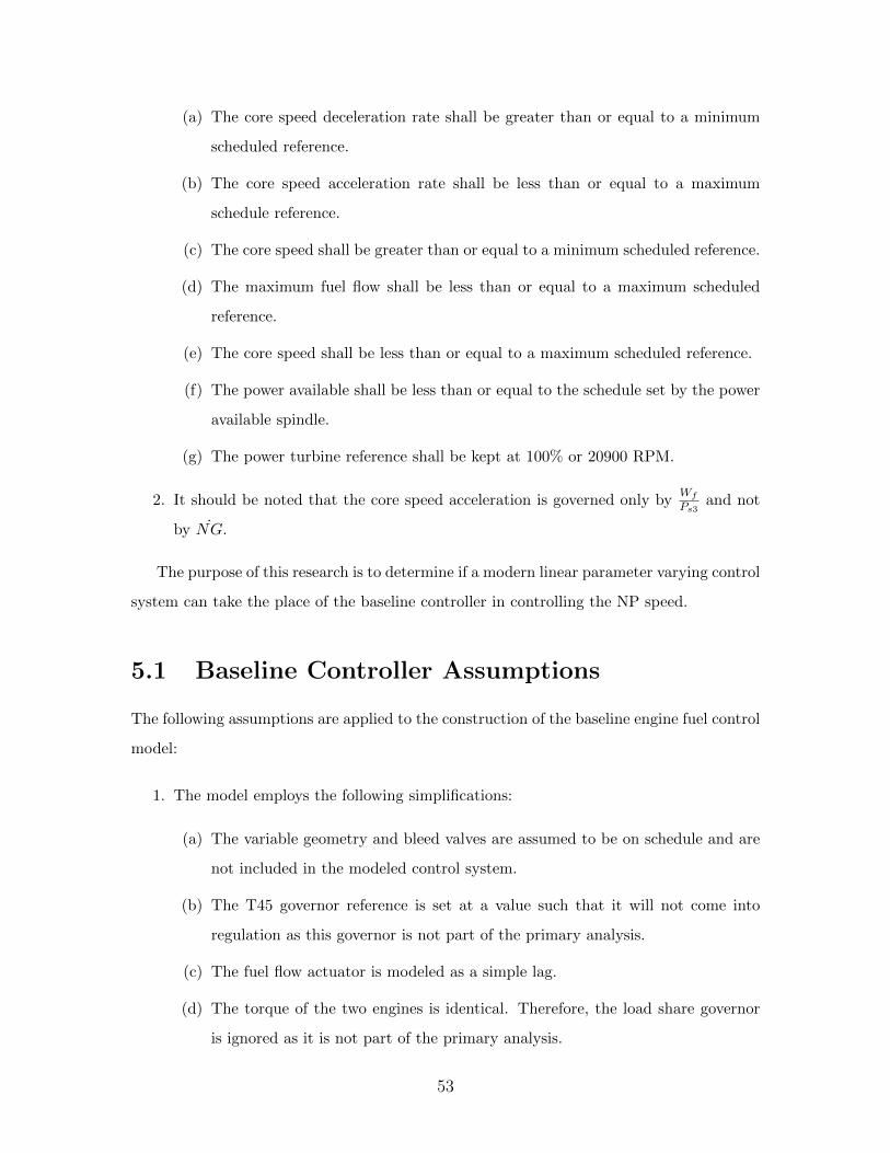
As mentioned above, the fuel flow is determined by the fuel control system by selecting
between several governors utilizing a priority scheme. Part of this selection logic is shown
in Figure 5-1 where WFIDM is the NG idle fuel flow bottoming reference, WFPAC is the
NG acceleration topping reference and WFPDM is the deceleration bottoming reference.
WFPDM incorporates the fuel flow topping, NG toppping and the NP governor. WFPDM
also includes the open loop collective based feedforward (Note: The feedforward logic is not
within the scope of this research). The collective lever is part of the rotorcraft that the
pilot uses to control the lift of the helicopter. The purpose of this research is to replace the
baseline NP governor with a linear parameter varying H∞ controller.
Figure 5-1: Fuel Flow Governor Selection
(The units of HMUSEL are in ratio units or WfPs3
)
54
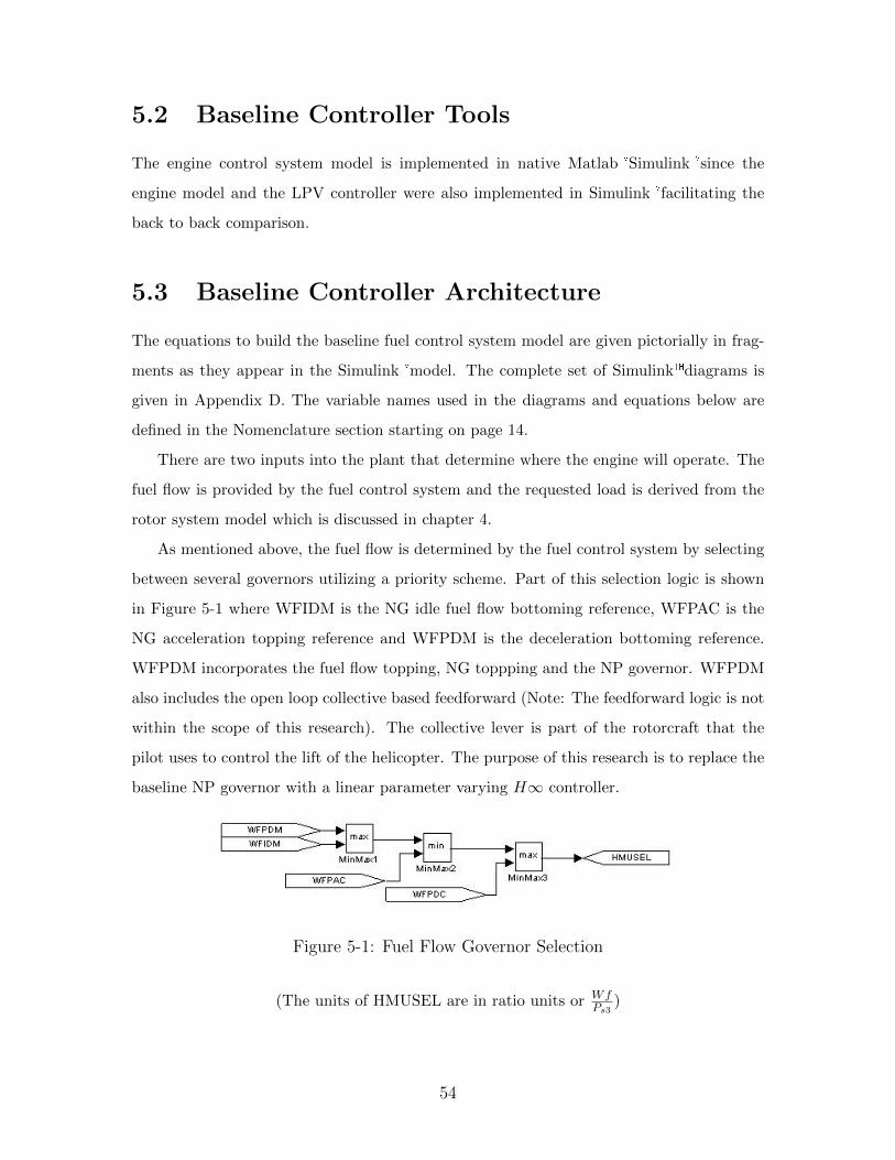
The NG idle fuel flow bottoming reference is defined in Figure 5-2. The plot and table
definitions for the 1-D linear interpolation labeled FHM5 HMUIdleSchedFunc1 in Figure 5-
2 is Figure F-6 and Table F.6 respectively. The plot and table definitions for the 1-D linear
interpolation labeled FHM6 HMUIdleSchedFunc2 in Figure 5-2 is Figure F-7 and Table F.7
respectively.
Figure 5-2: NG Idle Fuel Flow Governor
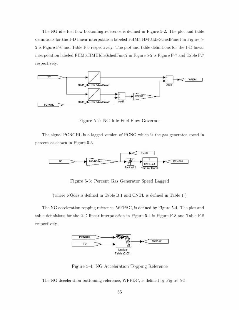
The signal PCNGHL is a lagged version of PCNG which is the gas generator speed in
percent as shown in Figure 5-3.
Figure 5-3: Percent Gas Generator Speed Lagged
(where NGdes is defined in Table B.1 and CNTL is defined in Table 1 )
The NG acceleration topping reference, WFPAC, is defined by Figure 5-4. The plot and
table definitions for the 2-D linear interpolation in Figure 5-4 is Figure F-8 and Table F.8
respectively.
Figure 5-4: NG Acceleration Topping Reference
The NG deceleration bottoming reference, WFPDC, is defined by Figure 5-5.
55
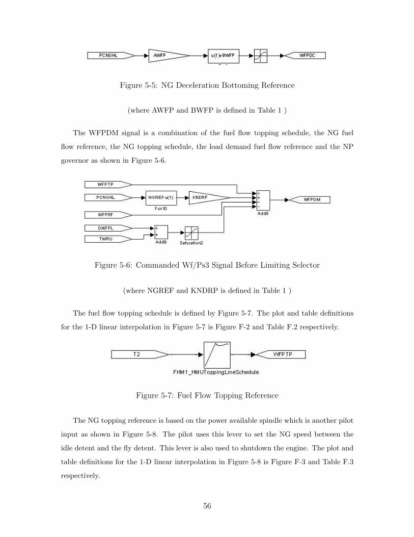
Figure 5-5: NG Deceleration Bottoming Reference
(where AWFP and BWFP is defined in Table 1 )
The WFPDM signal is a combination of the fuel flow topping schedule, the NG fuel
flow reference, the NG topping schedule, the load demand fuel flow reference and the NP
governor as shown in Figure 5-6.
Figure 5-6: Commanded Wf/Ps3 Signal Before Limiting Selector
(where NGREF and KNDRP is defined in Table 1 )
The fuel flow topping schedule is defined by Figure 5-7. The plot and table definitions
for the 1-D linear interpolation in Figure 5-7 is Figure F-2 and Table F.2 respectively.
Figure 5-7: Fuel Flow Topping Reference
The NG topping reference is based on the power available spindle which is another pilot
input as shown in Figure 5-8. The pilot uses this lever to set the NG speed between the
idle detent and the fly detent. This lever is also used to shutdown the engine. The plot and
table definitions for the 1-D linear interpolation in Figure 5-8 is Figure F-3 and Table F.3
respectively.
56
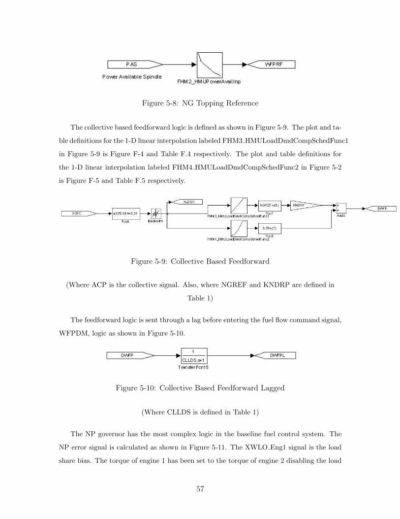
Figure 5-8: NG Topping Reference
The collective based feedforward logic is defined as shown in Figure 5-9. The plot and ta-
ble definitions for the 1-D linear interpolation labeled FHM3 HMULoadDmdCompSchedFunc1
in Figure 5-9 is Figure F-4 and Table F.4 respectively. The plot and table definitions for
the 1-D linear interpolation labeled FHM4 HMULoadDmdCompSchedFunc2 in Figure 5-2
is Figure F-5 and Table F.5 respectively.
Figure 5-9: Collective Based Feedforward
(Where ACP is the collective signal. Also, where NGREF and KNDRP are defined in
Table 1)
The feedforward logic is sent through a lag before entering the fuel flow command signal,
WFPDM, logic as shown in Figure 5-10.
Figure 5-10: Collective Based Feedforward Lagged
(Where CLLDS is defined in Table 1)
The NP governor has the most complex logic in the baseline fuel control system. The
NP error signal is calculated as shown in Figure 5-11. The XWLO Eng1 signal is the load
share bias. The torque of engine 1 has been set to the torque of engine 2 disabling the load
57
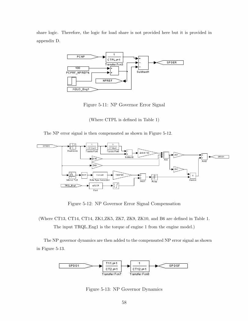
share logic. Therefore, the logic for load share is not provided here but it is provided in
appendix D.
Figure 5-11: NP Governor Error Signal
(Where CTPL is defined in Table 1)
The NP error signal is then compensated as shown in Figure 5-12.
Figure 5-12: NP Governor Error Signal Compensation
(Where CT13, CT14, CT14, ZK1,ZK5, ZK7, ZK9, ZK10, and B6 are defined in Table 1.
The input TRQL Eng1 is the torque of engine 1 from the engine model.)
The NP governor dynamics are then added to the compensated NP error signal as shown
in Figure 5-13.
Figure 5-13: NP Governor Dynamics
58
(Where T11, CT2, and CT12 are defined in Table 1)
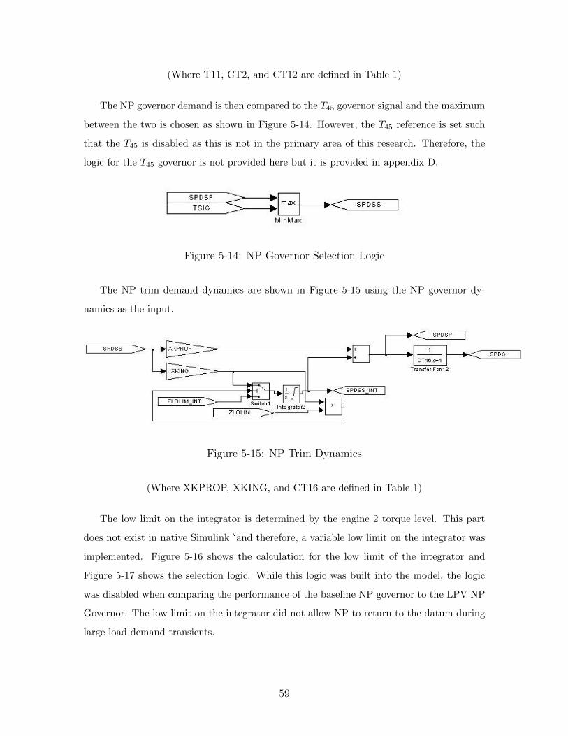
The NP governor demand is then compared to the T45 governor signal and the maximum
between the two is chosen as shown in Figure 5-14. However, the T45 reference is set such
that the T45 is disabled as this is not in the primary area of this research. Therefore, the
logic for the T45 governor is not provided here but it is provided in appendix D.
Figure 5-14: NP Governor Selection Logic
The NP trim demand dynamics are shown in Figure 5-15 using the NP governor dy-
namics as the input.
Figure 5-15: NP Trim Dynamics
(Where XKPROP, XKING, and CT16 are defined in Table 1)
The low limit on the integrator is determined by the engine 2 torque level. This part
does not exist in native Simulink�and therefore, a variable low limit on the integrator was
implemented. Figure 5-16 shows the calculation for the low limit of the integrator and
Figure 5-17 shows the selection logic. While this logic was built into the model, the logic
was disabled when comparing the performance of the baseline NP governor to the LPV NP
Governor. The low limit on the integrator did not allow NP to return to the datum during
large load demand transients.
59
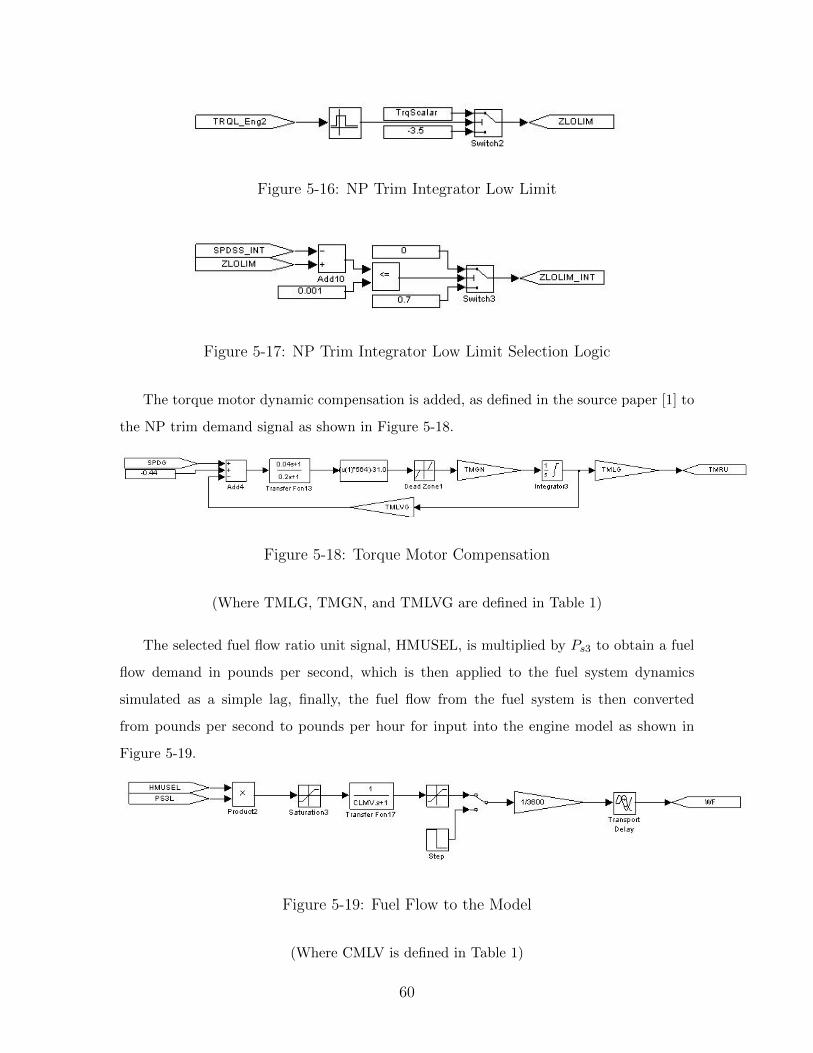
Figure 5-16: NP Trim Integrator Low Limit
Figure 5-17: NP Trim Integrator Low Limit Selection Logic
The torque motor dynamic compensation is added, as defined in the source paper [1] to
the NP trim demand signal as shown in Figure 5-18.
Figure 5-18: Torque Motor Compensation
(Where TMLG, TMGN, and TMLVG are defined in Table 1)
The selected fuel flow ratio unit signal, HMUSEL, is multiplied by Ps3 to obtain a fuel
flow demand in pounds per second, which is then applied to the fuel system dynamics
simulated as a simple lag, finally, the fuel flow from the fuel system is then converted
from pounds per second to pounds per hour for input into the engine model as shown in
Figure 5-19.
Figure 5-19: Fuel Flow to the Model
(Where CMLV is defined in Table 1)
60
5.4 Baseline Controller Validation
The baseline fuel control system is validated utilizing two transient cases provided in ref-
erence [1]. Figure 11 of reference [1] is a collective load disturbance while Figure 12 of the
reference paper provides a cyclic disturbance. The distinction between the two is important
to the engine control system. Currently, most helicopter engine control systems have knowl-
edge of the collective lever which is proportional to part of the load demand. However, there
are other factors that impact the rotor load such as cyclic movement, pedal movement, or
ambient conditions such as wind. Movement of the collective lever is called a compensated
maneuver due to the fact that engine control system reads the collective position and, in an
open loop fashion, adjusts the fuel flow in anticipation of the load application. Movement
of the cyclic or pedals is considered an uncompensated maneuver since the engine control
system does not have knowledge of the transient before the application of load. In this case,
the transient is driven solely from the error of the NP signal from the datum.
Figure 11 of reference [1] shows a collective pull producing a torque disturbance of about
40 ft-lbs with the engine model connected to the Sikorsky UH60A GENHEL rotor system
compared to flight test data. In this case, the aircraft is flying at approximately 90 knots.
However, the ambient pressures and temperatures are not provided. It should be noted that
the model prepared for this research does not include installed effects and therefore, does
not include the engine impacts due to ram air at the engine inlet. In addition, the rotor
system used in this research is much simpler than a typical rotor system model.
Since the ambient conditions were not disclosed, they were estimated by attempting to
match the core speed at the given fuel flow. It should also be noted that it is assumed
that there was an error in the labeling to the total torque parameter and that it should
have been “TOT.TORQUE, ft− lbsX10−1”. The T700 engines modeled for this research
are not capable of producing 12,000 ft-lbs or 1/2 of the 24,000 ft-lbs shown as the baseline
torque in Figure 11. The engine in the model is capable of providing approximately 460
ft-lbs at 100% NG and 100% NP speeds on a standard day at sea level. Finally, it should
be noted that the collective to load relationship is arbitrary, as discussed in chapter 4, for
this research while this relationship is modeled from the UH60A GENHEL model in the
reference paper.
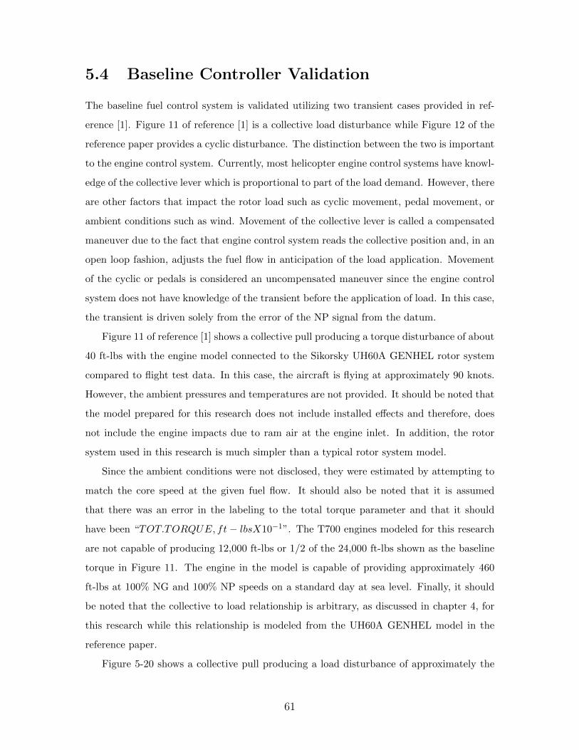
Figure 5-20 shows a collective pull producing a load disturbance of approximately the
61
same magnitude as Figure 11 in the reference paper. The ambient pressure is set to 12.2
psia which corresponds to 5,000 feet on a standard day. The ambient temperature is set
to 518.67◦R. These parameters were adjusted in an attempt to match the transient in the
reference paper.
0 2 4 6 8280
300
320
340
360
380
400
420
sec
Wf (
pph)
0 2 4 6 899.5
100
100.5
101
secN
P (
%)
0 2 4 6 889
89.5
90
90.5
91
91.5
92
92.5
sec
PC
NG
(%
)
0 2 4 6 8200
220
240
260
280
300
sec
TO
RQ
45 (
ft−lb
s)
SimulinkPaper
SimulinkPaper
SimulinkPaper
SimulinkPaper
Figure 5-20: Baseline Controller Validation - Collective Pull
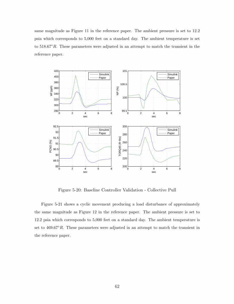
Figure 5-21 shows a cyclic movement producing a load disturbance of approximately
the same magnitude as Figure 12 in the reference paper. The ambient pressure is set to
12.2 psia which corresponds to 5,000 feet on a standard day. The ambient temperature is
set to 469.67◦R. These parameters were adjusted in an attempt to match the transient in
the reference paper.
62
−2 0 2 4 6 8280
300
320
340
360
380
400
sec
Wf (
pph)
0 2 4 6 898
98.2
98.4
98.6
98.8
sec
NP
(%
)
0 2 4 6 889.2
89.4
89.6
89.8
90
90.2
sec
PC
NG
(%
)
−2 0 2 4 6 8180
190
200
210
220
230
sec
TO
RQ
45 (
ft−lb
s)
SimulinkPaper
SimulinkPaper
SimulinkPaper
SimulinkPaper
Figure 5-21: Baseline Controller Validation - Cyclic Disturbance
While the two transients do not match absolutely, they do match fairly well dynamically.
In other words, the shape of the model response is very similar as well as the delta magnitude
for each of the parameters. Given the assumptions required to produce the transients and
the fact that the aircraft installation effects are not modeled, the match was considered
sufficient for the purposes of this research.
63
Chapter 6
Linear Parameter Varying (LPV)
Control Theory
6.1 Classical Approach
The classic approach to digital engine control design is to develop a non-linear model,
linearize that model at periodic core speed points, develop a controller for each linear point
and then interpolate or “gain schedule” between the LTI controllers as shown in Figure 6-1.
64
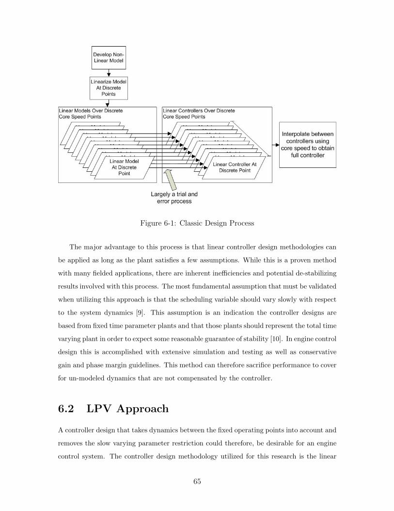
Figure 6-1: Classic Design Process
The major advantage to this process is that linear controller design methodologies can
be applied as long as the plant satisfies a few assumptions. While this is a proven method
with many fielded applications, there are inherent inefficiencies and potential de-stabilizing
results involved with this process. The most fundamental assumption that must be validated
when utilizing this approach is that the scheduling variable should vary slowly with respect
to the system dynamics [9]. This assumption is an indication the controller designs are
based from fixed time parameter plants and that those plants should represent the total time
varying plant in order to expect some reasonable guarantee of stability [10]. In engine control
design this is accomplished with extensive simulation and testing as well as conservative
gain and phase margin guidelines. This method can therefore sacrifice performance to cover
for un-modeled dynamics that are not compensated by the controller.
6.2 LPV Approach
A controller design that takes dynamics between the fixed operating points into account and
removes the slow varying parameter restriction could therefore, be desirable for an engine
control system. The controller design methodology utilized for this research is the linear
65
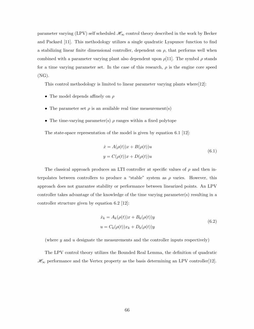
parameter varying (LPV) self scheduled H∞ control theory described in the work by Becker
and Packard [11]. This methodology utilizes a single quadratic Lyapunov function to find
a stabilizing linear finite dimensional controller, dependent on ρ, that performs well when
combined with a parameter varying plant also dependent upon ρ[11]. The symbol ρ stands
for a time varying parameter set. In the case of this research, ρ is the engine core speed
(NG).
This control methodology is limited to linear parameter varying plants where[12]:
� The model depends affinely on ρ
� The parameter set ρ is an available real time measurement(s)
� The time-varying parameter(s) ρ ranges within a fixed polytope
The state-space representation of the model is given by equation 6.1 [12]:
x = A(ρ(t))x+B(ρ(t))u
y = C(ρ(t))x+D(ρ(t))u(6.1)
The classical approach produces an LTI controller at specific values of ρ and then in-
terpolates between controllers to produce a “stable” system as ρ varies. However, this
approach does not guarantee stability or performance between linearized points. An LPV
controller takes advantage of the knowledge of the time varying parameter(s) resulting in a
controller structure given by equation 6.2 [12]:
xk = Ak(ρ(t))x+Bk(ρ(t))y
u = Ck(ρ(t))xk +Dk(ρ(t))y(6.2)
(where y and u designate the measurements and the controller inputs respectively)
The LPV control theory utilizes the Bounded Real Lemma, the definition of quadratic
H∞ performance and the Vertex property as the basis determining an LPV controller[12].
66
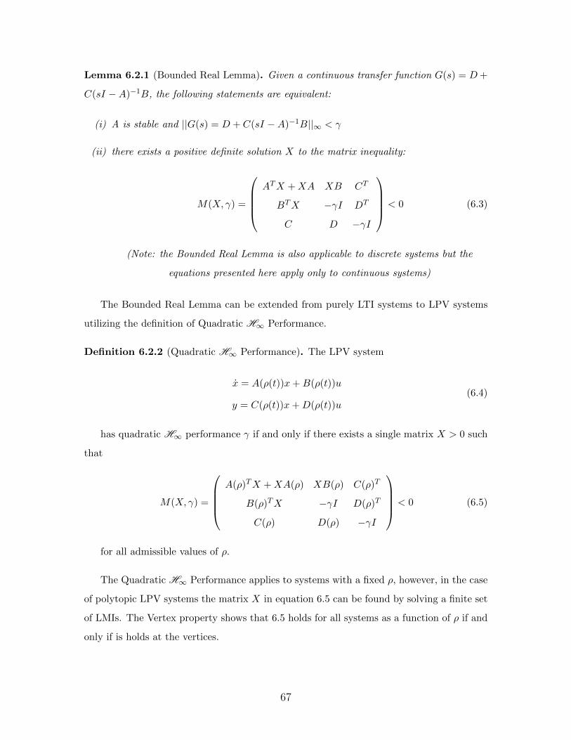
Lemma 6.2.1 (Bounded Real Lemma). Given a continuous transfer function G(s) = D+
C(sI −A)−1B, the following statements are equivalent:
(i) A is stable and ||G(s) = D + C(sI −A)−1B||∞ < γ
(ii) there exists a positive definite solution X to the matrix inequality:
M(X, γ) =
ATX +XA XB CT
BTX −γI DT
C D −γI
< 0 (6.3)
(Note: the Bounded Real Lemma is also applicable to discrete systems but the
equations presented here apply only to continuous systems)
The Bounded Real Lemma can be extended from purely LTI systems to LPV systems
utilizing the definition of Quadratic H∞ Performance.
Definition 6.2.2 (Quadratic H∞ Performance). The LPV system
x = A(ρ(t))x+B(ρ(t))u
y = C(ρ(t))x+D(ρ(t))u(6.4)
has quadratic H∞ performance γ if and only if there exists a single matrix X > 0 such
that
M(X, γ) =
A(ρ)TX +XA(ρ) XB(ρ) C(ρ)T
B(ρ)TX −γI D(ρ)T
C(ρ) D(ρ) −γI
< 0 (6.5)
for all admissible values of ρ.
The Quadratic H∞ Performance applies to systems with a fixed ρ, however, in the case
of polytopic LPV systems the matrix X in equation 6.5 can be found by solving a finite set
of LMIs. The Vertex property shows that 6.5 holds for all systems as a function of ρ if and
only if is holds at the vertices.
67
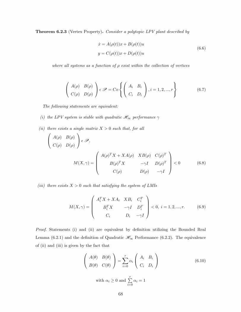
Theorem 6.2.3 (Vertex Property). Consider a polytopic LPV plant described by
x = A(ρ(t))x+B(ρ(t))u
y = C(ρ(t))x+D(ρ(t))u(6.6)
where all systems as a function of ρ exist within the collection of vertices
A(ρ) B(ρ)
C(ρ) D(ρ)
ε P = Co
Ai Bi
Ci Di
, i = 1, 2, ..., r
(6.7)
The following statements are equivalent:
(i) the LPV system is stable with quadratic H∞ performance γ
(ii) there exists a single matrix X > 0 such that, for all A(ρ) B(ρ)
C(ρ) D(ρ)
ε P,
M(X, γ) =
A(ρ)TX +XA(ρ) XB(ρ) C(ρ)T
B(ρ)TX −γI D(ρ)T
C(ρ) D(ρ) −γI
< 0 (6.8)
(iii) there exists X > 0 such that satisfying the system of LMIs
M(X, γ) =
AT
i X +XAi XBi CTi
BTi X −γI DT
i
Ci Di −γI
< 0, i = 1, 2, ..., r. (6.9)
Proof. Statements (i) and (ii) are equivalent by definition utilizing the Bounded Real
Lemma (6.2.1) and the definition of Quadratic H∞ Performance (6.2.2). The equivalence
of (ii) and (iii) is given by the fact that A(θ) B(θ)
B(θ) C(θ)
=
r∑i=0
αi
Ai Bi
Ci Di
(6.10)
with αi ≥ 0 andr∑
i=0αi = 1
68
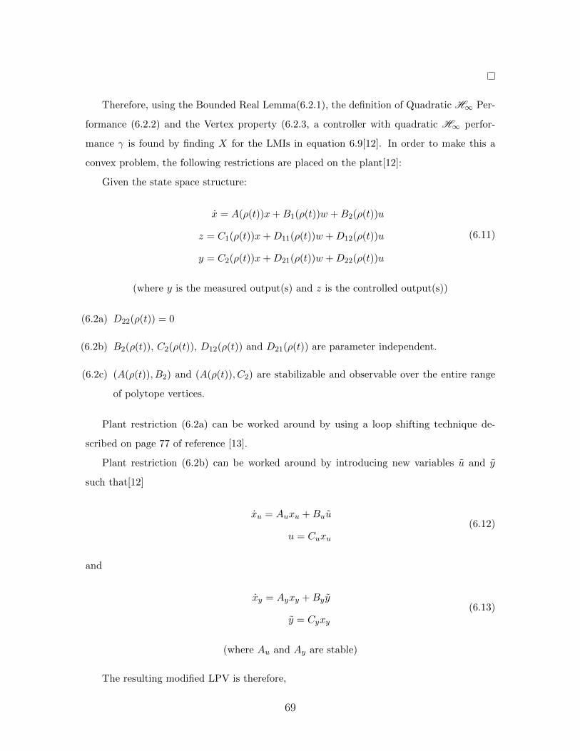
Therefore, using the Bounded Real Lemma(6.2.1), the definition of Quadratic H∞ Per-
formance (6.2.2) and the Vertex property (6.2.3, a controller with quadratic H∞ perfor-
mance γ is found by finding X for the LMIs in equation 6.9[12]. In order to make this a
convex problem, the following restrictions are placed on the plant[12]:
Given the state space structure:
x = A(ρ(t))x+B1(ρ(t))w +B2(ρ(t))u
z = C1(ρ(t))x+D11(ρ(t))w +D12(ρ(t))u
y = C2(ρ(t))x+D21(ρ(t))w +D22(ρ(t))u
(6.11)
(where y is the measured output(s) and z is the controlled output(s))
(6.2a) D22(ρ(t)) = 0
(6.2b) B2(ρ(t)), C2(ρ(t)), D12(ρ(t)) and D21(ρ(t)) are parameter independent.
(6.2c) (A(ρ(t)), B2) and (A(ρ(t)), C2) are stabilizable and observable over the entire range
of polytope vertices.
Plant restriction (6.2a) can be worked around by using a loop shifting technique de-
scribed on page 77 of reference [13].
Plant restriction (6.2b) can be worked around by introducing new variables u and y
such that[12]
xu = Auxu +Buu
u = Cuxu
(6.12)
and
xy = Ayxy +Byy
y = Cyxy
(6.13)
(where Au and Ay are stable)
The resulting modified LPV is therefore,
69
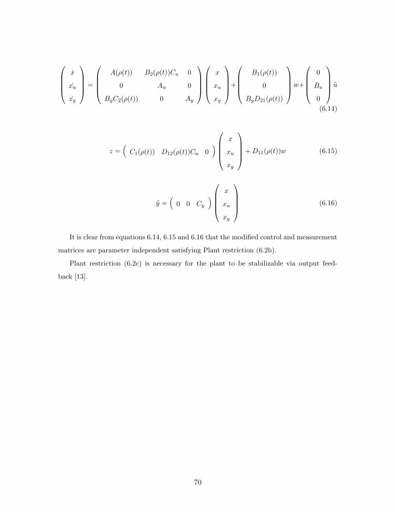
x
xu
xy
=
A(ρ(t)) B2(ρ(t))Cu 0
0 Au 0
ByC2(ρ(t)) 0 Ay
x
xu
xy
+
B1(ρ(t))
0
ByD21(ρ(t))
w+
0
Bu
0
u
(6.14)
z =(C1(ρ(t)) D12(ρ(t))Cu 0
)x
xu
xy
+D11(ρ(t))w (6.15)
y =(
0 0 Cy
)x
xu
xy
(6.16)
It is clear from equations 6.14, 6.15 and 6.16 that the modified control and measurement
matrices are parameter independent satisfying Plant restriction (6.2b).
Plant restriction (6.2c) is necessary for the plant to be stabilizable via output feed-
back [13].
70
Chapter 7
LPV Controller Design
7.1 LPV Controller Assumptions
The following are the LPV controller assumptions:
� The plant must satisfy the assumptions detailed in section 6.2. Since the B matrix is
parameter dependent, the methods described in [12] must be utilized.
� It is assumed that the baseline controller provided in reference [1] was sufficiently
tuned for this application.
� It is assumed that there is no model uncertainty. In practice, this must be included
for robustness.
7.2 LPV Controller Tools
The LPV controller design described in this chapter is accomplished using the Matlab�LMI
control toolbox developed by Pascal Gahinet, Arkadi Nemirovski, Alan J. Laub and Mahout
Chilli [2]. There are several commands that were critical in the development of the LPV
controller for this research: “ltisys”, “psys”, “sconnect” and “hinfgs”. Descriptions of these
commands are provided in appendix G.1. The “ltisys” command packs the state-space
matrices A, B, C, D, and E into a single system matrix readable by the LMI toolbox. The
“psys” command takes the packed system matrices created by the “ltisys” command and
produces a polytopic model that can be referenced by “hinfgs”. The “sconnect” command
71
sets up the structure for the “hinfgs” command such that the inputs and outputs of the
controller are appropriately indicated. The “hinfgs” command takes the polytopic system
model and produces a gain scheduled H∞ controller.
In addition to the tools used to create the controller, the pdsimul command is used to
simulate the controller along parameter trajectories. The description for this command is
also provided in appendix G.1.
7.2.1 Changes to LMI toolset to deal with polytopic model
The pdsimul command was used to validate the controller against the linear plant. However,
as stated in the command description in appendix G.1 it was only designed for affine systems.
However, with a slight modification the code for pdsimul and the dependent function polsim,
it is possible to utilize these commands for the polytopic system in this research. The code
changes are provided in appendix G.3. To avoid confusion, the functions were renamed
from pdsimul and polsim to t700pdsimul and t700polsim respectively.
7.3 LPV Controller Architecture
The linearized plants obtained in section 3.5 have the following state space equation form:
x =
˙NP
˙P45
˙Ps3
˙P41
˙NG
= A
NP
P45
Ps3
P41
NG
︸ ︷︷ ︸
x
+B
Wf
Qref
︸ ︷︷ ︸
u
y =
Qpt
NP
NG%
˙NG
= C
NP
P45
Ps3
P41
NG
︸ ︷︷ ︸
x
+D
Wf
Qref
︸ ︷︷ ︸
u
(7.1)
72
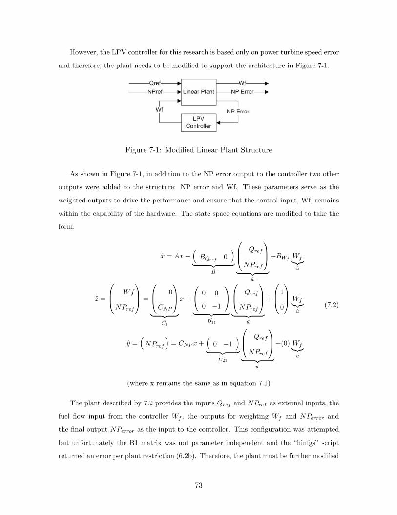
However, the LPV controller for this research is based only on power turbine speed error
and therefore, the plant needs to be modified to support the architecture in Figure 7-1.
Figure 7-1: Modified Linear Plant Structure
As shown in Figure 7-1, in addition to the NP error output to the controller two other
outputs were added to the structure: NP error and Wf. These parameters serve as the
weighted outputs to drive the performance and ensure that the control input, Wf, remains
within the capability of the hardware. The state space equations are modified to take the
form:
x = Ax+(BQref 0
)︸ ︷︷ ︸
B
Qref
NPref
︸ ︷︷ ︸
w
+BWfWf︸︷︷︸u
z =
Wf
NPref
=
0
CNP
︸ ︷︷ ︸
C1
x+
0 0
0 −1
︸ ︷︷ ︸
D11
Qref
NPref
︸ ︷︷ ︸
w
+
1
0
Wf︸︷︷︸u
y =(NPref
)= CNPx+
(0 −1
)︸ ︷︷ ︸
D21
Qref
NPref
︸ ︷︷ ︸
w
+(0) Wf︸︷︷︸u
(7.2)
(where x remains the same as in equation 7.1)
The plant described by 7.2 provides the inputs Qref and NPref as external inputs, the
fuel flow input from the controller Wf , the outputs for weighting Wf and NPerror and
the final output NPerror as the input to the controller. This configuration was attempted
but unfortunately the B1 matrix was not parameter independent and the “hinfgs” script
returned an error per plant restriction (6.2b). Therefore, the plant must be further modified
73
as described in section 6.2. The state-space equations are further modified to produce a
pseudo-parameter independent B matrix as shown in equation 7.3. x
˙u
=
A BWf
0 −a
︸ ︷︷ ︸
A
x
u
+
BQref 0
0 0
︸ ︷︷ ︸
B
Qref
NPref
︸ ︷︷ ︸
w
+
0
1
Wf︸︷︷︸u
z =
Wf
NPref
=
0 0
CNP 0
︸ ︷︷ ︸
C1
x
u
+
0 0
0 −1
︸ ︷︷ ︸
D11
Qref
NPref
︸ ︷︷ ︸
w
+
1
0
Wf︸︷︷︸u
y =(NPref
)=(CNP 0
)x
u
+(
0 −1)
︸ ︷︷ ︸D21
Qref
NPref
︸ ︷︷ ︸
w
+(0) Wf︸︷︷︸u
(7.3)
(where x remains the same as in equation 7.1)
The state space equation 7.3 parameter dependent vector BWfis now part of the mod-
ified A matrix satisfying plant restriction (6.2b). The consequence is that a new parameter
is introduced u with the dynamics of a low pass filter with a corner at a.
˙u = u− au (7.4)
or
us = u− au (7.5)
which when rearranged provides the transfer function from u to u:
u
u=
1
s+ a(7.6)
The input point for the linear plant obtained in section 3.5 is the output WF shown in
Figure 5-19. The dynamics of the fuel flow actuator is a low pass filter of the form:
u
u=
1
CLMV ∗ s+ 1(7.7)
(where CLMV is defined in Table E)
74
Therefore, to include the fuel flow actuator dynamics as part of the modified plant the
structure in equation 7.3 is changed to:
x
˙u
=
A BWf
0 −1
︸ ︷︷ ︸
A
x
u
+
BQref 0
0 0
︸ ︷︷ ︸
B
Qref
NPref
︸ ︷︷ ︸
w
+
0
CLMV
Wf︸︷︷︸u
z =
Wf
NPref
=
0 0
CNP 0
︸ ︷︷ ︸
C1
x
u
+
0 0
0 −1
︸ ︷︷ ︸
D11
Qref
NPref
︸ ︷︷ ︸
w
+
1
0
Wf︸︷︷︸u
y =(NPref
)=(CNP 0
)x
u
+(
0 −1)
︸ ︷︷ ︸D21
Qref
NPref
︸ ︷︷ ︸
w
+(0) Wf︸︷︷︸u
(7.8)
(where x remains the same as in equation 7.1)
At this point, the modified plant is ready for the application of the weighting functions
which will determine the performance of the controller. In this case, the desired performance
is good disturbance rejection, fuel flow actuator commands appropriate for the hardware,
and zero steady state error. Therefore, the weighting function on the error signal should
be a low pass filter to achieve good steady state performance. The controller weighting
function on the other hand should be a high pass filter to penalize high frequencies and
keep the bandwidth of the control signal within the capabilities of the hardware.
We(s) =(10−3s+ 1)
(10−1s+ 1)(7.9)
(where We is the NP error weighting function)
Wc(s) =(10−2s+ 1)
(10−4s+ 1)(7.10)
(where Wc is the control input weighting function)
Once the weighting functions have been added to the modified plant, the LPV controller
must be setup using the sconnect command which indicates to the hinfgs command the plant
75
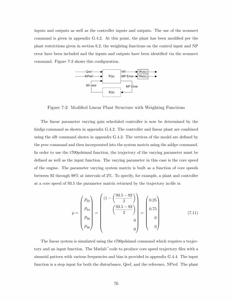
inputs and outputs as well as the controller inputs and outputs. The use of the sconnect
command is given in appendix G.4.2. At this point, the plant has been modified per the
plant restrictions given in section 6.2, the weighting functions on the control input and NP
error have been included and the inputs and outputs have been identified via the sconnect
command. Figure 7-2 shows this configuration.
Figure 7-2: Modified Linear Plant Structure with Weighting Functions
The linear parameter varying gain scheduled controller is now be determined by the
hinfgs command as shown in appendix G.4.2. The controller and linear plant are combined
using the slft command shown in appendix G.4.3. The vertices of the model are defined by
the pvec command and then incorporated into the system matrix using the addpv command.
In order to use the t700pdsimul function, the trajectory of the varying parameter must be
defined as well as the input function. The varying parameter in this case is the core speed
of the engine. The parameter varying system matrix is built as a function of core speeds
between 92 through 98% at intervals of 2%. To specify, for example, a plant and controller
at a core speed of 93.5 the parameter matrix returned by the trajectory m-file is:
p =
P92
P94
P96
P98
=
(1−(
93.5− 92
2
)(
93.5− 92
2
)0
0
=
0.25
0.75
0
0
(7.11)
The linear system is simulated using the t700pdsimul command which requires a trajec-
tory and an input function. The Matlab�code to produce core speed trajectory files with a
sinusoid pattern with various frequencies and bias is provided in appendix G.4.4. The input
function is a step input for both the disturbance, Qref, and the reference, NPref. The plant
76
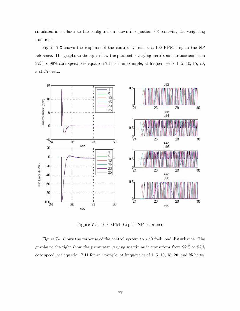
simulated is set back to the configuration shown in equation 7.3 removing the weighting
functions.
Figure 7-3 shows the response of the control system to a 100 RPM step in the NP
reference. The graphs to the right show the parameter varying matrix as it transitions from
92% to 98% core speed, see equation 7.11 for an example, at frequencies of 1, 5, 10, 15, 20,
and 25 hertz.
Figure 7-3: 100 RPM Step in NP reference
Figure 7-4 shows the response of the control system to a 40 ft-lb load disturbance. The
graphs to the right show the parameter varying matrix as it transitions from 92% to 98%
core speed, see equation 7.11 for an example, at frequencies of 1, 5, 10, 15, 20, and 25 hertz.
77
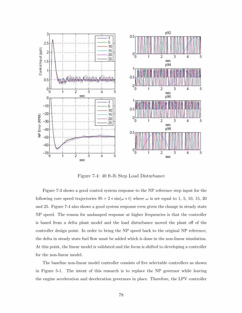
Figure 7-4: 40 ft-lb Step Load Disturbance
Figure 7-3 shows a good control system response to the NP reference step input for the
following core speed trajectories 95 + 2 ∗ sin(ω ∗ t) where ω is set equal to 1, 5, 10, 15, 20
and 25. Figure 7-4 also shows a good system response even given the change in steady state
NP speed. The reason for undamped response at higher frequencies is that the controller
is based from a delta plant model and the load disturbance moved the plant off of the
controller design point. In order to bring the NP speed back to the original NP reference,
the delta in steady state fuel flow must be added which is done in the non-linear simulation.
At this point, the linear model is validated and the focus is shifted to developing a controller
for the non-linear model.
The baseline non-linear model controller consists of five selectable controllers as shown
in Figure 5-1. The intent of this research is to replace the NP governor while leaving
the engine acceleration and deceleration governors in place. Therefore, the LPV controller
78
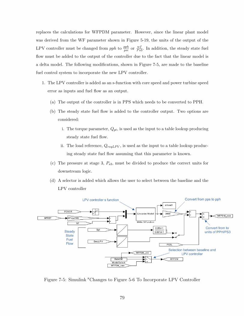
replaces the calculations for WFPDM parameter. However, since the linear plant model
was derived from the WF parameter shown in Figure 5-19, the units of the output of the
LPV controller must be changed from pph to pphpsi or wf
Ps3 . In addition, the steady state fuel
flow must be added to the output of the controller due to the fact that the linear model is
a delta model. The following modifications, shown in Figure 7-5, are made to the baseline
fuel control system to incorporate the new LPV controller.
1. The LPV controller is added as an s-function with core speed and power turbine speed
error as inputs and fuel flow as an output.
(a) The output of the controller is in PPS which needs to be converted to PPH.
(b) The steady state fuel flow is added to the controller output. Two options are
considered:
i. The torque parameter, Qpt, is used as the input to a table lookup producing
steady state fuel flow.
ii. The load reference, QreqLPV , is used as the input to a table lookup produc-
ing steady state fuel flow assuming that this parameter is known.
(c) The pressure at stage 3, Ps3, must be divided to produce the correct units for
downstream logic.
(d) A selector is added which allows the user to select between the baseline and the
LPV controller
Figure 7-5: Simulink�Changes to Figure 5-6 To Incorporate LPV Controller
79
The controller s-function is required due to the fact that there are no native Simulink�parts
that implement the LPV controller structure. However, the s-function is relatively straight
forward and is based from the Limited Integrator Level 1 M-File structure provided in the
basic Matlab�installation at "matlabroot\toolbox\Simulink\texttrademark\blocks\limintm.m".
The LPV controller, pdK, obtained via an m-file similar to the one provided in appendix G.4.2
except that the NG range is expanded to 76 to 100% is provided as an s-function parameter.
The following modifications are made to the base s-function:
1. The state space matrices are defined as global variables. This is due to the fact that
they are calculated during the derivative case.
2. The function “GetModel” is added which pulls the state space matrices from pdK.
3. The function “NGInputConversion” is added to produce the input necessary obtain
the model at the specified point.
4. The model is initialized with:
(a) The “GetModel” function is called at 92% NG.
(b) 2 inputs: NG and NP speed error
(c) 1 output: fuel flow
(d) The number of continuous states is set equal to the rows in the A matrix
(e) X0 is set to a vector of zeros the size of number of states
5. In the derivative case the “GetModel” function is called prior to calculating the
derivative.
6. The output case uses the state space matrices obtained in the derivative case to
calculate the output.
The LPV controller s-function is provided in appendix G.4.6.
7.4 LPV Controller Validation
The initial tuning of the LPV controller was performed during the linear controller design
analysis described in section 7.3. However, it was determined that additional tuning was
desired to achieve the following:
80
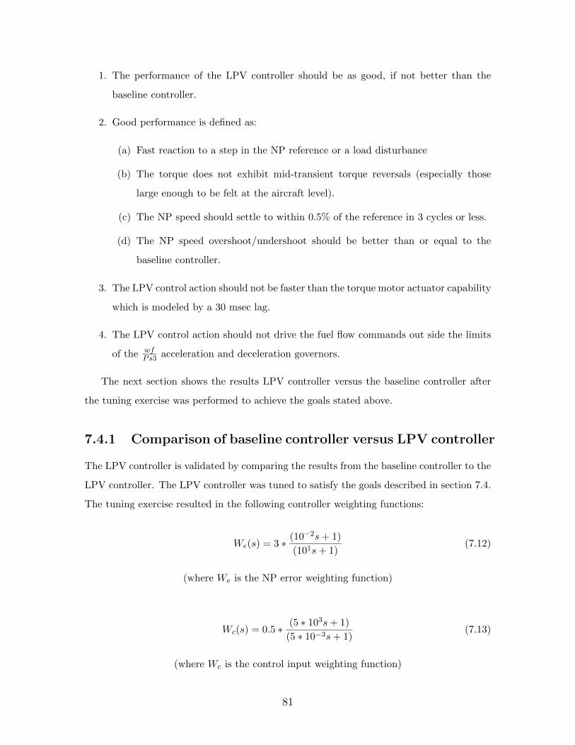
1. The performance of the LPV controller should be as good, if not better than the
baseline controller.
2. Good performance is defined as:
(a) Fast reaction to a step in the NP reference or a load disturbance
(b) The torque does not exhibit mid-transient torque reversals (especially those
large enough to be felt at the aircraft level).
(c) The NP speed should settle to within 0.5% of the reference in 3 cycles or less.
(d) The NP speed overshoot/undershoot should be better than or equal to the
baseline controller.
3. The LPV control action should not be faster than the torque motor actuator capability
which is modeled by a 30 msec lag.
4. The LPV control action should not drive the fuel flow commands out side the limits
of the wfPs3 acceleration and deceleration governors.
The next section shows the results LPV controller versus the baseline controller after
the tuning exercise was performed to achieve the goals stated above.
7.4.1 Comparison of baseline controller versus LPV controller
The LPV controller is validated by comparing the results from the baseline controller to the
LPV controller. The LPV controller was tuned to satisfy the goals described in section 7.4.
The tuning exercise resulted in the following controller weighting functions:
We(s) = 3 ∗ (10−2s+ 1)
(101s+ 1)(7.12)
(where We is the NP error weighting function)
Wc(s) = 0.5 ∗ (5 ∗ 103s+ 1)
(5 ∗ 10−3s+ 1)(7.13)
(where Wc is the control input weighting function)
81
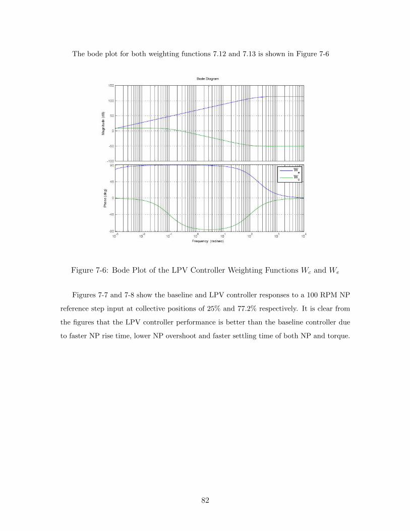
The bode plot for both weighting functions 7.12 and 7.13 is shown in Figure 7-6
Figure 7-6: Bode Plot of the LPV Controller Weighting Functions Wc and We
Figures 7-7 and 7-8 show the baseline and LPV controller responses to a 100 RPM NP
reference step input at collective positions of 25% and 77.2% respectively. It is clear from
the figures that the LPV controller performance is better than the baseline controller due
to faster NP rise time, lower NP overshoot and faster settling time of both NP and torque.
82
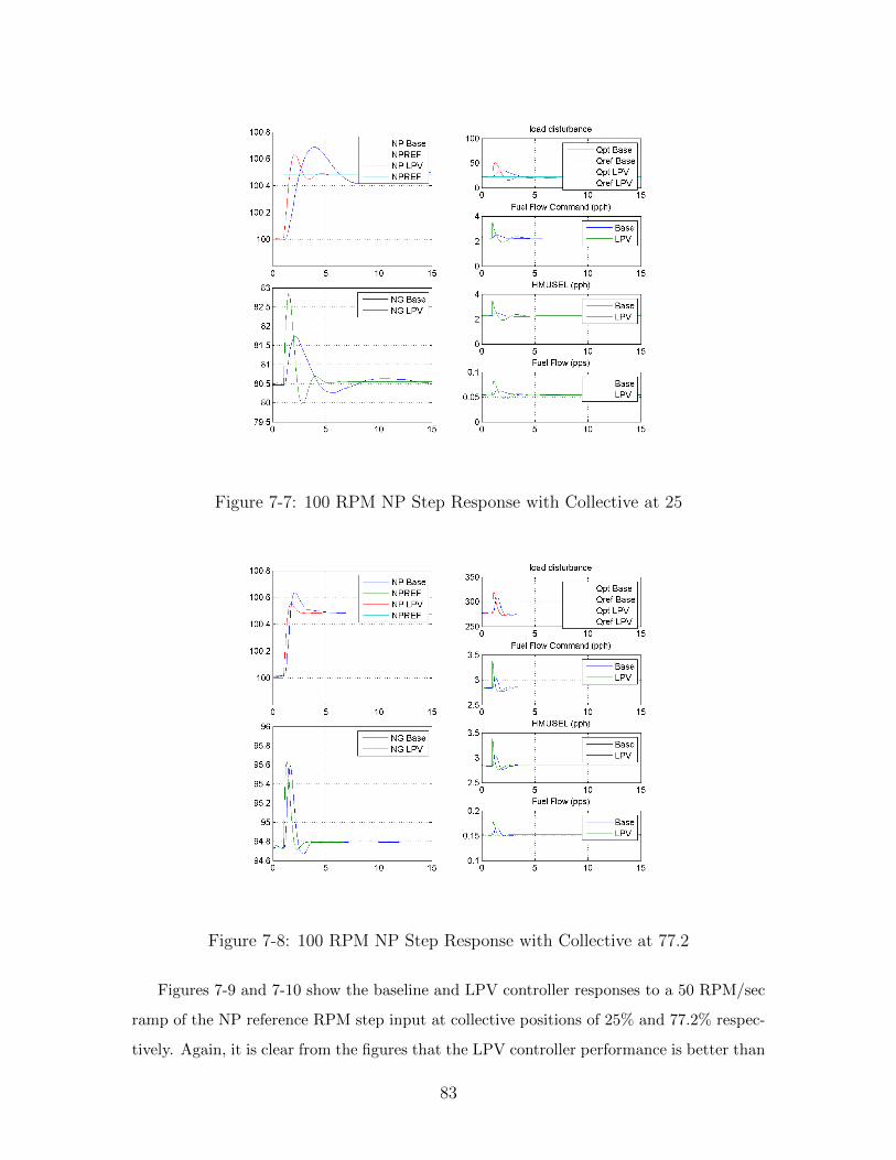
Figure 7-7: 100 RPM NP Step Response with Collective at 25
Figure 7-8: 100 RPM NP Step Response with Collective at 77.2
Figures 7-9 and 7-10 show the baseline and LPV controller responses to a 50 RPM/sec
ramp of the NP reference RPM step input at collective positions of 25% and 77.2% respec-
tively. Again, it is clear from the figures that the LPV controller performance is better than
83
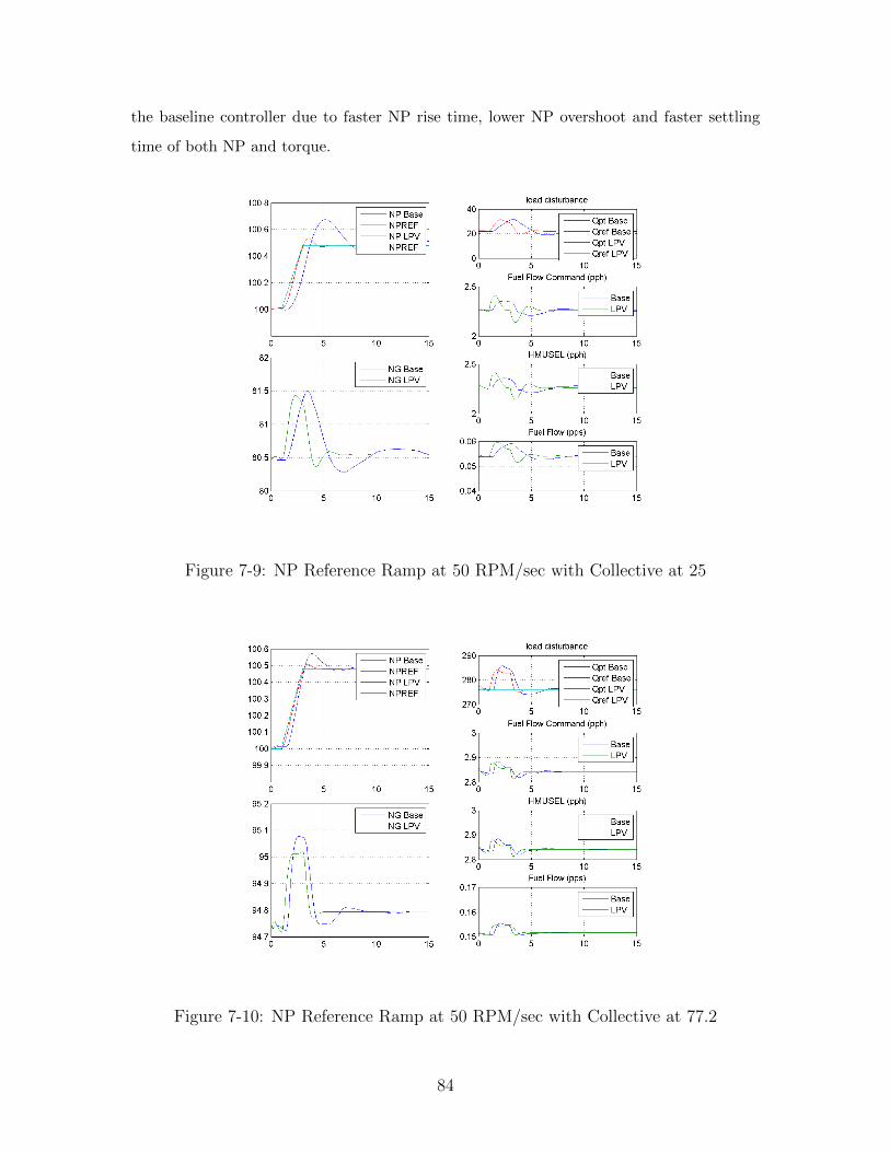
the baseline controller due to faster NP rise time, lower NP overshoot and faster settling
time of both NP and torque.
Figure 7-9: NP Reference Ramp at 50 RPM/sec with Collective at 25
Figure 7-10: NP Reference Ramp at 50 RPM/sec with Collective at 77.2
84
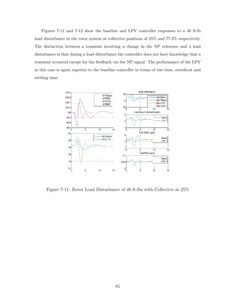
Figures 7-11 and 7-12 show the baseline and LPV controller responses to a 40 ft-lb
load disturbance in the rotor system at collective positions of 25% and 77.2% respectively.
The distinction between a transient involving a change in the NP reference and a load
disturbance is that during a load disturbance the controller does not have knowledge that a
transient occurred except for the feedback via the NP signal. The performance of the LPV
in this case is again superior to the baseline controller in terms of rise time, overshoot and
settling time.
Figure 7-11: Rotor Load Disturbance of 40 ft-lbs with Collective at 25%
85
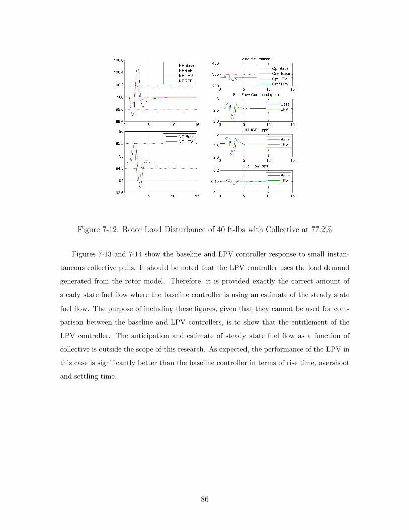
Figure 7-12: Rotor Load Disturbance of 40 ft-lbs with Collective at 77.2%
Figures 7-13 and 7-14 show the baseline and LPV controller response to small instan-
taneous collective pulls. It should be noted that the LPV controller uses the load demand
generated from the rotor model. Therefore, it is provided exactly the correct amount of
steady state fuel flow where the baseline controller is using an estimate of the steady state
fuel flow. The purpose of including these figures, given that they cannot be used for com-
parison between the baseline and LPV controllers, is to show that the entitlement of the
LPV controller. The anticipation and estimate of steady state fuel flow as a function of
collective is outside the scope of this research. As expected, the performance of the LPV in
this case is significantly better than the baseline controller in terms of rise time, overshoot
and settling time.
86
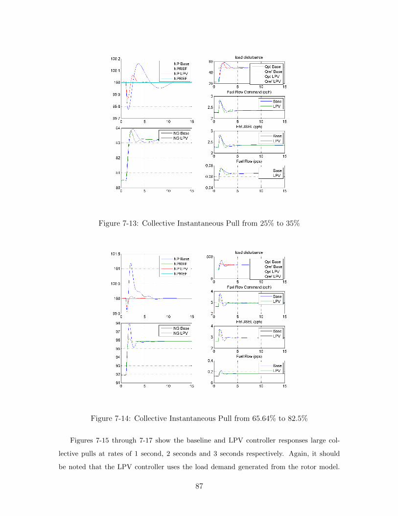
Figure 7-13: Collective Instantaneous Pull from 25% to 35%
Figure 7-14: Collective Instantaneous Pull from 65.64% to 82.5%
Figures 7-15 through 7-17 show the baseline and LPV controller responses large col-
lective pulls at rates of 1 second, 2 seconds and 3 seconds respectively. Again, it should
be noted that the LPV controller uses the load demand generated from the rotor model.
87
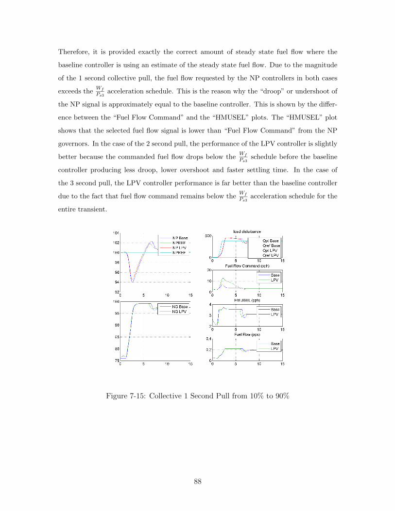
Therefore, it is provided exactly the correct amount of steady state fuel flow where the
baseline controller is using an estimate of the steady state fuel flow. Due to the magnitude
of the 1 second collective pull, the fuel flow requested by the NP controllers in both cases
exceeds theWf
Ps3acceleration schedule. This is the reason why the “droop” or undershoot of
the NP signal is approximately equal to the baseline controller. This is shown by the differ-
ence between the “Fuel Flow Command” and the “HMUSEL” plots. The “HMUSEL” plot
shows that the selected fuel flow signal is lower than “Fuel Flow Command” from the NP
governors. In the case of the 2 second pull, the performance of the LPV controller is slightly
better because the commanded fuel flow drops below theWf
Ps3schedule before the baseline
controller producing less droop, lower overshoot and faster settling time. In the case of
the 3 second pull, the LPV controller performance is far better than the baseline controller
due to the fact that fuel flow command remains below theWf
Ps3acceleration schedule for the
entire transient.
Figure 7-15: Collective 1 Second Pull from 10% to 90%
88
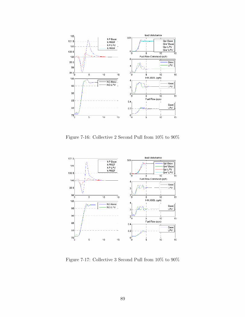
Figure 7-16: Collective 2 Second Pull from 10% to 90%
Figure 7-17: Collective 3 Second Pull from 10% to 90%
89
Chapter 8
Conclusions
The results in chapter 7 show that a LPV control system can be effectively applied to an
engine control system with positive results. In the cases of the NP step, NP ramp and load
disturbances the performance of the LPV controller is significantly better than the baseline
controller. With further tuning of the baseline controller, it is most likely possible to obtain
the same performance as the LPV controller. However, it would most like require a more
significant tuning effort to cover the same range of engine torque conditions.
In retrospect, the linear tuning effort produces controller weighting functions that were
not very effective in the non-linear model. This was due mainly to the fact that the goals,
described in section 7.4 could not be tested using the linear model since it did not contain
the other fuel flow governors. However, the effort was not wasted since it did provide
validation of the LPV controller against the engine itself.
The LPV controller that produced the best results was the one where the linear plant
was simplified to contain only the rotor system pole. This pole is a lumped state that
includes the power turbine, gear box, main rotor and tail rotor. This pole is also the closest
to the jω axis. Without question, the P41 and P45 can be excluded since these poles are
very fast compared to the rotor system pole. There could be an argument to include the
NG and Ps3 parameters since they are close to the range of the rotor system pole and they
are measured parameters. The inclusion of these additional parameters would have to be
weighed against the increase complexity of the controller. The smaller the linear plant the
less complex the resulting controller which makes a production implementation easier. This
research did not show an improvement in controller performance with these states included
90
in the linear plant.
The fact that the rotor system is modeled by a single lumped state also impacts the
complexity of the controller. In a practical application, the rotor system should be modeled
to a much higher fidelity to include the natural frequencies and damping of both the main
and tail rotors. However, the methods used to create the LPV controller can easily be
applied to a more complex plant without changes to the algorithm.
8.1 Future Work
This research does not attempt to address the anticipation and estimate of the steady state
fuel flow based on helicopter load demands signals. In a practical application, the exact
load demand of the rotor system is not known and must be estimated using these signals
mainly the collective signal. However, in practice the linear analysis and tuning of the NP
governor is performed outside of the tuning of the anticipation logic and therefore, it was
valid to neglect this for the scope of this research.
This research assumes no model uncertainty and therefore, in a practical application
this would have to be addressed. In addition, the concept of stability for the baseline con-
troller is based on gain margin and phase margin which the aerospace industry is familiar
and comfortable with. It may be necessary to produce equivalent gain and phase margin
assessments to obtain acceptance from the certification authorities.
The LPV controller did not attempt to limit the output when the acceleration or de-
celeration governors are selected. Therefore, as shown in 7-15 there is the potential for
the controller to windup. The performance of the governor could be improved if additional
”anti-windup” logic is incorporated.
91
Appendix A
Engine Model Diagrams
92
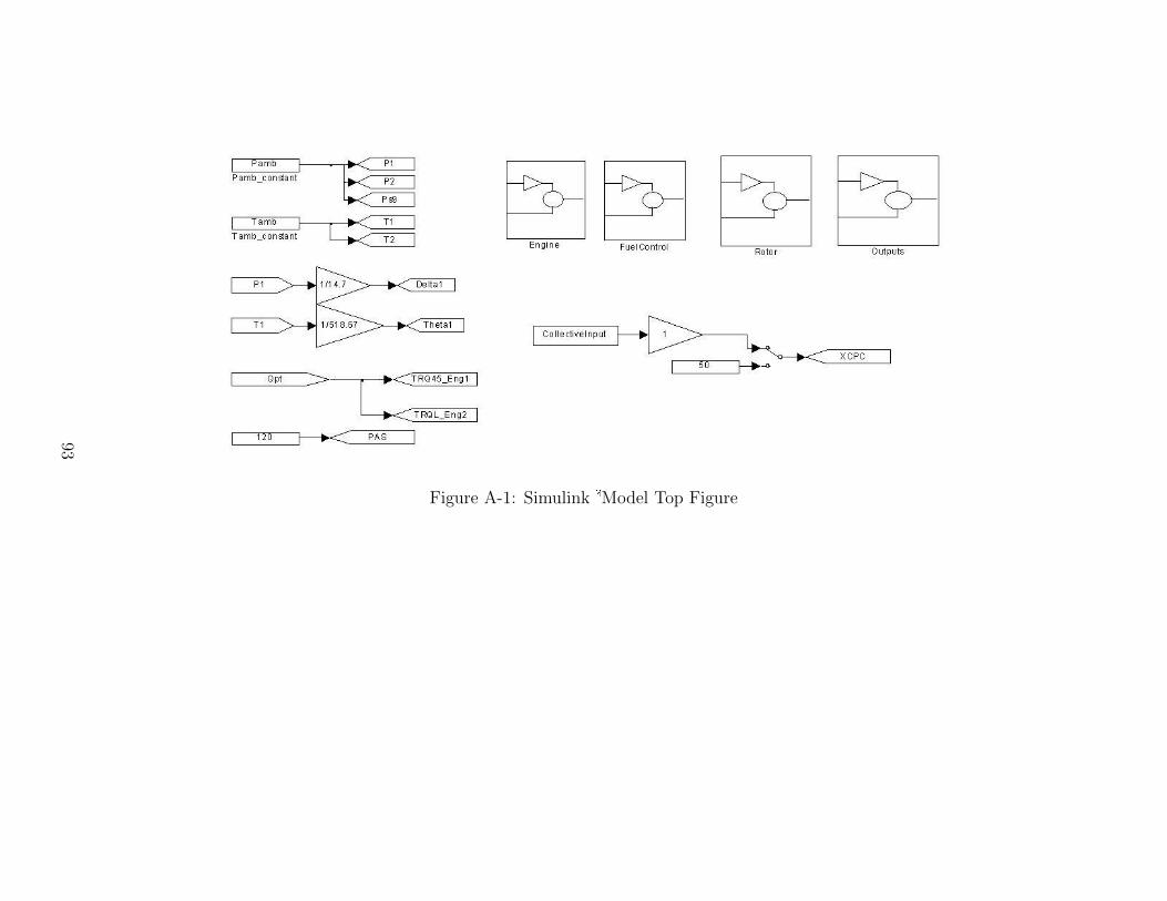
Figure A-1: Simulink�Model Top Figure
93
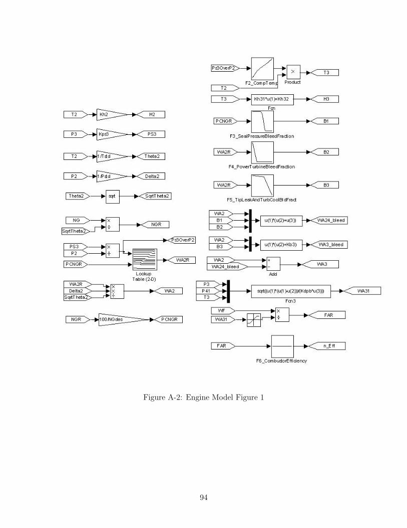
Figure A-2: Engine Model Figure 1
94
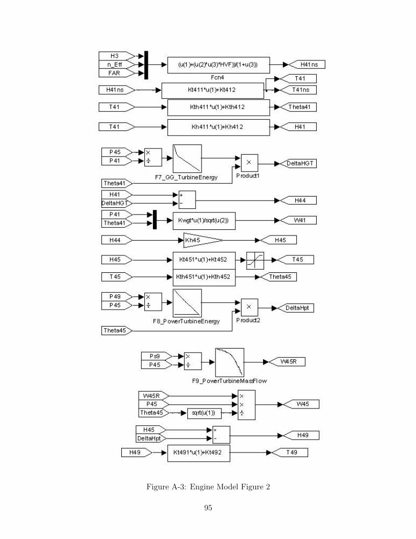
Figure A-3: Engine Model Figure 2
95
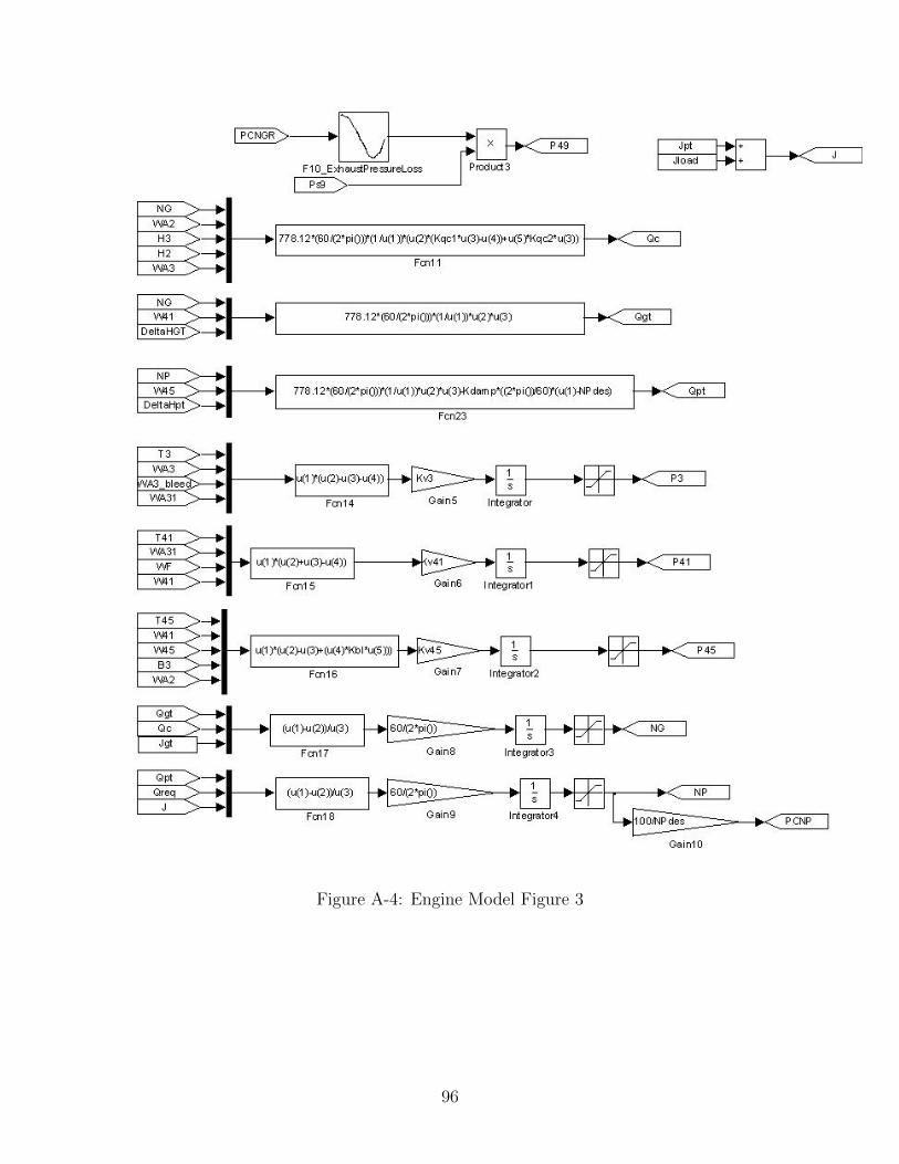
Figure A-4: Engine Model Figure 3
96
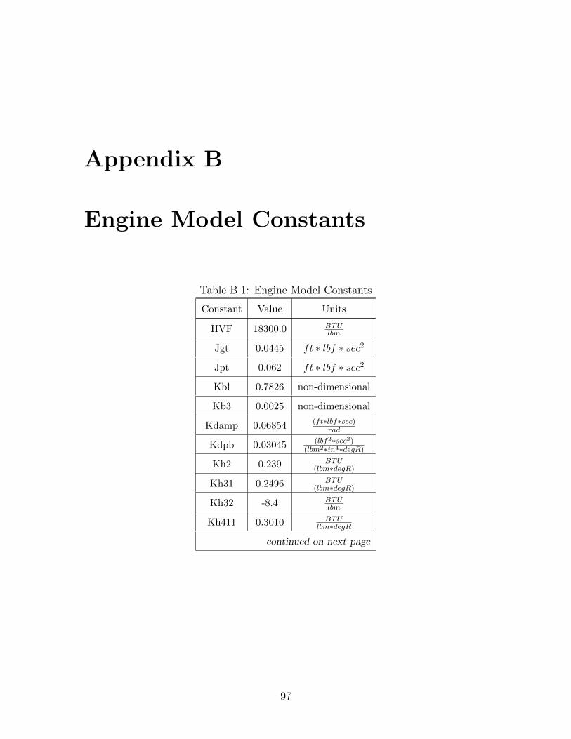
Appendix B
Engine Model Constants
Table B.1: Engine Model Constants
Constant Value Units
HVF 18300.0 BTUlbm
Jgt 0.0445 ft ∗ lbf ∗ sec2
Jpt 0.062 ft ∗ lbf ∗ sec2
Kbl 0.7826 non-dimensional
Kb3 0.0025 non-dimensional
Kdamp 0.06854 (ft∗lbf∗sec)rad
Kdpb 0.03045 (lbf2∗sec2)(lbm2∗in4∗degR)
Kh2 0.239 BTU(lbm∗degR)
Kh31 0.2496 BTU(lbm∗degR)
Kh32 -8.4 BTUlbm
Kh411 0.3010 BTUlbm∗degR
continued on next page
97
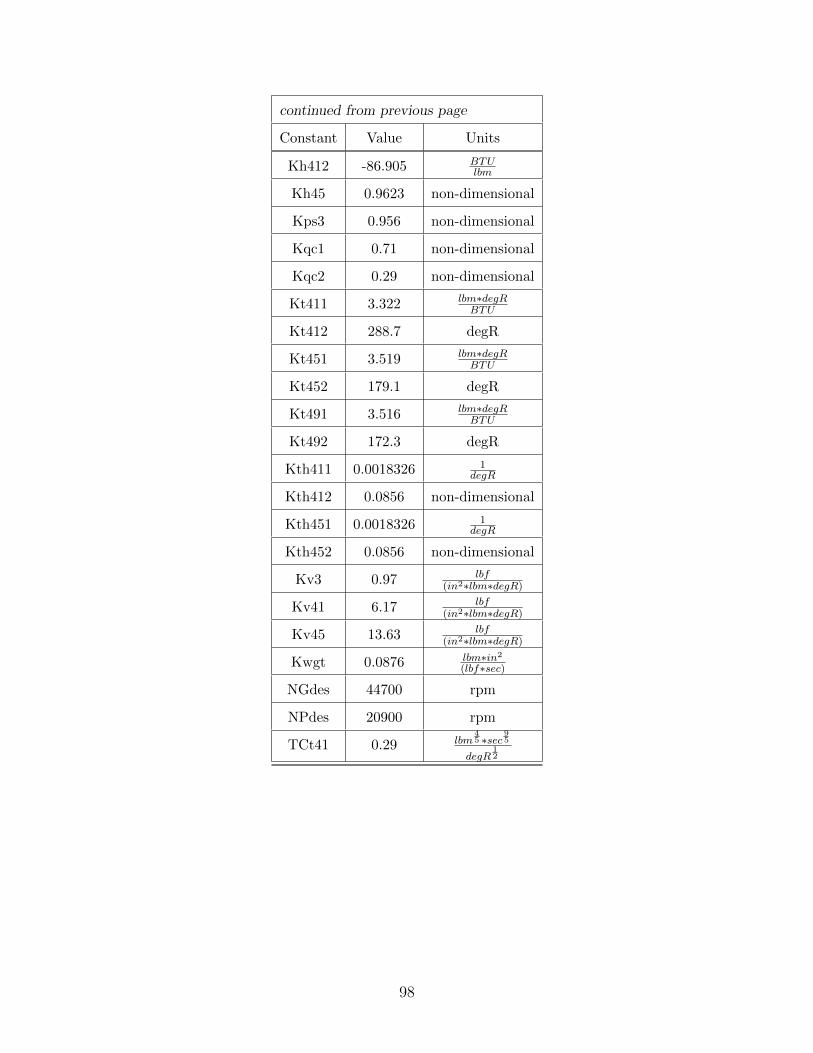
continued from previous page
Constant Value Units
Kh412 -86.905 BTUlbm
Kh45 0.9623 non-dimensional
Kps3 0.956 non-dimensional
Kqc1 0.71 non-dimensional
Kqc2 0.29 non-dimensional
Kt411 3.322 lbm∗degRBTU
Kt412 288.7 degR
Kt451 3.519 lbm∗degRBTU
Kt452 179.1 degR
Kt491 3.516 lbm∗degRBTU
Kt492 172.3 degR
Kth411 0.0018326 1degR
Kth412 0.0856 non-dimensional
Kth451 0.0018326 1degR
Kth452 0.0856 non-dimensional
Kv3 0.97 lbf(in2∗lbm∗degR)
Kv41 6.17 lbf(in2∗lbm∗degR)
Kv45 13.63 lbf(in2∗lbm∗degR)
Kwgt 0.0876 lbm∗in2
(lbf∗sec)
NGdes 44700 rpm
NPdes 20900 rpm
TCt41 0.29 lbm45 ∗sec
95
degR12
98

Appendix C
Engine Model Schedules
99
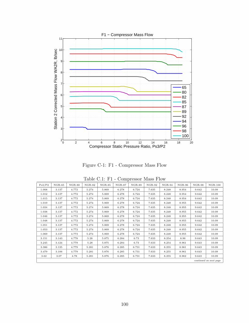
0 2 4 6 8 10 12 14 16 18 202
3
4
5
6
7
8
9
10
11
Compressor Static Pressure Ratio, Ps3/P2
Sta
tion
2 C
orre
cted
Mas
s F
low
WA
2R, l
b/se
c
F1 − Compressor Mass Flow
65808285878992949698100
Figure C-1: F1 - Compressor Mass Flow
Table C.1: F1 - Compressor Mass FlowPs3/P2 NGR-65 NGR-80 NGR-82 NGR-85 NGR-87 NGR-89 NGR-92 NGR-94 NGR-96 NGR-98 NGR-100
1.008 3.137 4.772 5.274 5.869 6.278 6.724 7.635 8.248 8.954 9.642 10.09
1.012 3.137 4.772 5.274 5.869 6.278 6.724 7.635 8.248 8.954 9.642 10.09
1.015 3.137 4.772 5.274 5.869 6.278 6.724 7.635 8.248 8.954 9.642 10.09
1.019 3.137 4.772 5.274 5.869 6.278 6.724 7.635 8.248 8.955 9.642 10.09
1.024 3.137 4.772 5.274 5.869 6.278 6.724 7.635 8.248 8.955 9.642 10.09
1.038 3.137 4.772 5.274 5.869 6.278 6.724 7.635 8.248 8.955 9.642 10.09
1.046 3.137 4.772 5.274 5.869 6.278 6.724 7.635 8.248 8.955 9.642 10.09
1.048 3.137 4.772 5.274 5.869 6.278 6.724 7.635 8.248 8.955 9.642 10.09
1.051 3.137 4.772 5.274 5.869 6.278 6.724 7.635 8.248 8.955 9.642 10.09
1.053 3.137 4.772 5.274 5.869 6.278 6.724 7.635 8.248 8.955 9.642 10.09
1.069 3.137 4.773 5.274 5.869 6.278 6.724 7.635 8.248 8.955 9.642 10.09
3.151 3.143 4.778 5.28 5.875 6.284 6.73 7.633 8.254 8.96 9.643 10.09
3.245 3.124 4.779 5.28 5.875 6.284 6.73 7.633 8.254 8.961 9.643 10.09
3.386 3.125 4.779 5.281 5.876 6.285 6.731 7.633 8.255 8.961 9.643 10.09
3.479 3.106 4.779 5.281 5.876 6.285 6.731 7.633 8.255 8.961 9.643 10.09
3.62 3.07 4.78 5.281 5.876 6.285 6.731 7.633 8.255 8.962 9.643 10.09
continued on next page
100
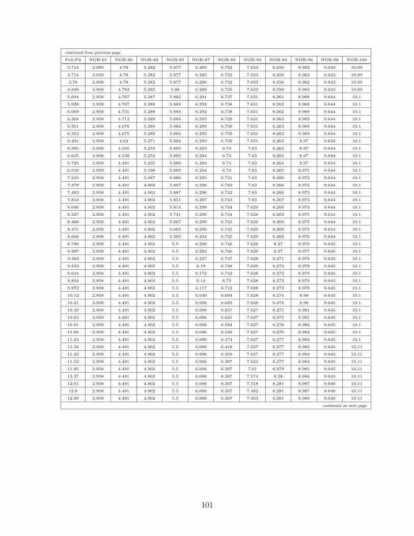
continued from previous page
Ps3/P2 NGR-65 NGR-80 NGR-82 NGR-85 NGR-87 NGR-89 NGR-92 NGR-94 NGR-96 NGR-98 NGR-100
3.714 2.995 4.78 5.282 5.877 6.285 6.732 7.633 8.256 8.962 9.643 10.09
3.714 3.033 4.78 5.282 5.877 6.285 6.732 7.633 8.256 8.962 9.643 10.09
3.76 2.958 4.78 5.282 5.877 6.286 6.732 7.633 8.256 8.962 9.643 10.09
4.849 2.958 4.783 5.285 5.88 6.289 6.735 7.632 8.259 8.965 9.643 10.09
5.694 2.958 4.767 5.287 5.882 6.291 6.737 7.631 8.261 8.968 9.644 10.1
5.928 2.958 4.767 5.288 5.883 6.292 6.738 7.631 8.262 8.968 9.644 10.1
6.069 2.958 4.731 5.288 5.883 6.292 6.738 7.631 8.262 8.969 9.644 10.1
6.304 2.958 4.713 5.289 5.884 6.293 6.739 7.631 8.263 8.969 9.644 10.1
6.351 2.958 4.676 5.289 5.884 6.293 6.739 7.631 8.263 8.969 9.644 10.1
6.353 2.958 4.675 5.289 5.884 6.293 6.739 7.631 8.263 8.969 9.644 10.1
6.491 2.958 4.62 5.271 5.884 6.293 6.739 7.631 8.263 8.97 9.644 10.1
6.585 2.958 4.565 5.259 5.885 6.293 6.74 7.63 8.264 8.97 9.644 10.1
6.635 2.958 4.538 5.253 5.885 6.294 6.74 7.63 8.264 8.97 9.644 10.1
6.725 2.958 4.491 5.235 5.885 6.294 6.74 7.63 8.264 8.97 9.644 10.1
6.916 2.958 4.491 5.198 5.885 6.294 6.74 7.63 8.265 8.971 9.644 10.1
7.245 2.958 4.491 5.087 5.886 6.295 6.741 7.63 8.266 8.972 9.644 10.1
7.478 2.958 4.491 4.902 5.887 6.296 6.742 7.63 8.266 8.973 9.644 10.1
7.483 2.958 4.491 4.902 5.887 6.296 6.742 7.63 8.266 8.973 9.644 10.1
7.812 2.958 4.491 4.902 5.851 6.297 6.743 7.63 8.267 8.973 9.644 10.1
8.046 2.958 4.491 4.902 5.814 6.298 6.744 7.629 8.268 8.974 9.644 10.1
8.327 2.958 4.491 4.902 5.741 6.298 6.744 7.629 8.269 8.975 9.644 10.1
8.468 2.958 4.491 4.902 5.667 6.299 6.745 7.629 8.269 8.975 9.644 10.1
8.471 2.958 4.491 4.902 5.665 6.299 6.745 7.629 8.269 8.975 9.644 10.1
8.608 2.958 4.491 4.902 5.593 6.294 6.745 7.629 8.269 8.976 9.644 10.1
8.796 2.958 4.491 4.902 5.5 6.288 6.746 7.629 8.27 8.976 9.645 10.1
8.987 2.958 4.491 4.902 5.5 6.282 6.746 7.629 8.27 8.977 9.645 10.1
9.363 2.958 4.491 4.902 5.5 6.227 6.747 7.628 8.271 8.978 9.645 10.1
9.553 2.958 4.491 4.902 5.5 6.19 6.748 7.628 8.272 8.978 9.645 10.1
9.644 2.958 4.491 4.902 5.5 6.172 6.742 7.628 8.272 8.979 9.645 10.1
9.834 2.958 4.491 4.902 5.5 6.14 6.73 7.628 8.273 8.979 9.645 10.1
9.972 2.958 4.491 4.902 5.5 6.117 6.712 7.628 8.273 8.979 9.645 10.1
10.12 2.958 4.491 4.902 5.5 6.049 6.694 7.628 8.274 8.98 9.645 10.1
10.21 2.958 4.491 4.902 5.5 6.006 6.685 7.628 8.274 8.98 9.645 10.1
10.49 2.958 4.491 4.902 5.5 6.006 6.657 7.627 8.275 8.981 9.645 10.1
10.63 2.958 4.491 4.902 5.5 6.006 6.621 7.627 8.275 8.981 9.645 10.1
10.91 2.958 4.491 4.902 5.5 6.006 6.584 7.627 8.276 8.982 9.645 10.1
11.05 2.958 4.491 4.902 5.5 6.006 6.548 7.627 8.276 8.982 9.645 10.1
11.24 2.958 4.491 4.902 5.5 6.006 6.474 7.627 8.277 8.983 9.645 10.1
11.34 2.958 4.491 4.902 5.5 6.006 6.418 7.627 8.277 8.983 9.645 10.11
11.43 2.958 4.491 4.902 5.5 6.006 6.359 7.627 8.277 8.984 9.645 10.11
11.52 2.958 4.491 4.902 5.5 6.006 6.307 7.624 8.277 8.984 9.645 10.11
11.95 2.958 4.491 4.902 5.5 6.006 6.307 7.61 8.279 8.985 9.645 10.11
12.37 2.958 4.491 4.902 5.5 6.006 6.307 7.574 8.28 8.986 9.645 10.11
12.61 2.958 4.491 4.902 5.5 6.006 6.307 7.518 8.281 8.987 9.646 10.11
12.8 2.958 4.491 4.902 5.5 6.006 6.307 7.482 8.281 8.987 9.646 10.11
12.89 2.958 4.491 4.902 5.5 6.006 6.307 7.453 8.281 8.988 9.646 10.11
continued on next page
101
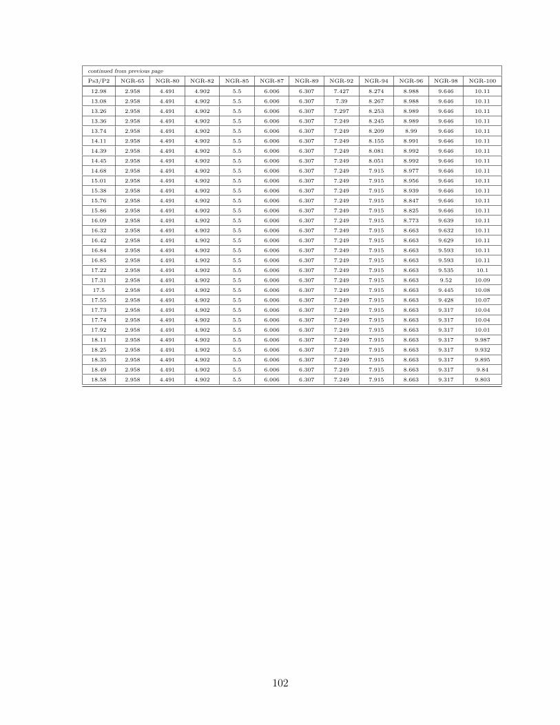
continued from previous page
Ps3/P2 NGR-65 NGR-80 NGR-82 NGR-85 NGR-87 NGR-89 NGR-92 NGR-94 NGR-96 NGR-98 NGR-100
12.98 2.958 4.491 4.902 5.5 6.006 6.307 7.427 8.274 8.988 9.646 10.11
13.08 2.958 4.491 4.902 5.5 6.006 6.307 7.39 8.267 8.988 9.646 10.11
13.26 2.958 4.491 4.902 5.5 6.006 6.307 7.297 8.253 8.989 9.646 10.11
13.36 2.958 4.491 4.902 5.5 6.006 6.307 7.249 8.245 8.989 9.646 10.11
13.74 2.958 4.491 4.902 5.5 6.006 6.307 7.249 8.209 8.99 9.646 10.11
14.11 2.958 4.491 4.902 5.5 6.006 6.307 7.249 8.155 8.991 9.646 10.11
14.39 2.958 4.491 4.902 5.5 6.006 6.307 7.249 8.081 8.992 9.646 10.11
14.45 2.958 4.491 4.902 5.5 6.006 6.307 7.249 8.051 8.992 9.646 10.11
14.68 2.958 4.491 4.902 5.5 6.006 6.307 7.249 7.915 8.977 9.646 10.11
15.01 2.958 4.491 4.902 5.5 6.006 6.307 7.249 7.915 8.956 9.646 10.11
15.38 2.958 4.491 4.902 5.5 6.006 6.307 7.249 7.915 8.939 9.646 10.11
15.76 2.958 4.491 4.902 5.5 6.006 6.307 7.249 7.915 8.847 9.646 10.11
15.86 2.958 4.491 4.902 5.5 6.006 6.307 7.249 7.915 8.825 9.646 10.11
16.09 2.958 4.491 4.902 5.5 6.006 6.307 7.249 7.915 8.773 9.639 10.11
16.32 2.958 4.491 4.902 5.5 6.006 6.307 7.249 7.915 8.663 9.632 10.11
16.42 2.958 4.491 4.902 5.5 6.006 6.307 7.249 7.915 8.663 9.629 10.11
16.84 2.958 4.491 4.902 5.5 6.006 6.307 7.249 7.915 8.663 9.593 10.11
16.85 2.958 4.491 4.902 5.5 6.006 6.307 7.249 7.915 8.663 9.593 10.11
17.22 2.958 4.491 4.902 5.5 6.006 6.307 7.249 7.915 8.663 9.535 10.1
17.31 2.958 4.491 4.902 5.5 6.006 6.307 7.249 7.915 8.663 9.52 10.09
17.5 2.958 4.491 4.902 5.5 6.006 6.307 7.249 7.915 8.663 9.445 10.08
17.55 2.958 4.491 4.902 5.5 6.006 6.307 7.249 7.915 8.663 9.428 10.07
17.73 2.958 4.491 4.902 5.5 6.006 6.307 7.249 7.915 8.663 9.317 10.04
17.74 2.958 4.491 4.902 5.5 6.006 6.307 7.249 7.915 8.663 9.317 10.04
17.92 2.958 4.491 4.902 5.5 6.006 6.307 7.249 7.915 8.663 9.317 10.01
18.11 2.958 4.491 4.902 5.5 6.006 6.307 7.249 7.915 8.663 9.317 9.987
18.25 2.958 4.491 4.902 5.5 6.006 6.307 7.249 7.915 8.663 9.317 9.932
18.35 2.958 4.491 4.902 5.5 6.006 6.307 7.249 7.915 8.663 9.317 9.895
18.49 2.958 4.491 4.902 5.5 6.006 6.307 7.249 7.915 8.663 9.317 9.84
18.58 2.958 4.491 4.902 5.5 6.006 6.307 7.249 7.915 8.663 9.317 9.803
102
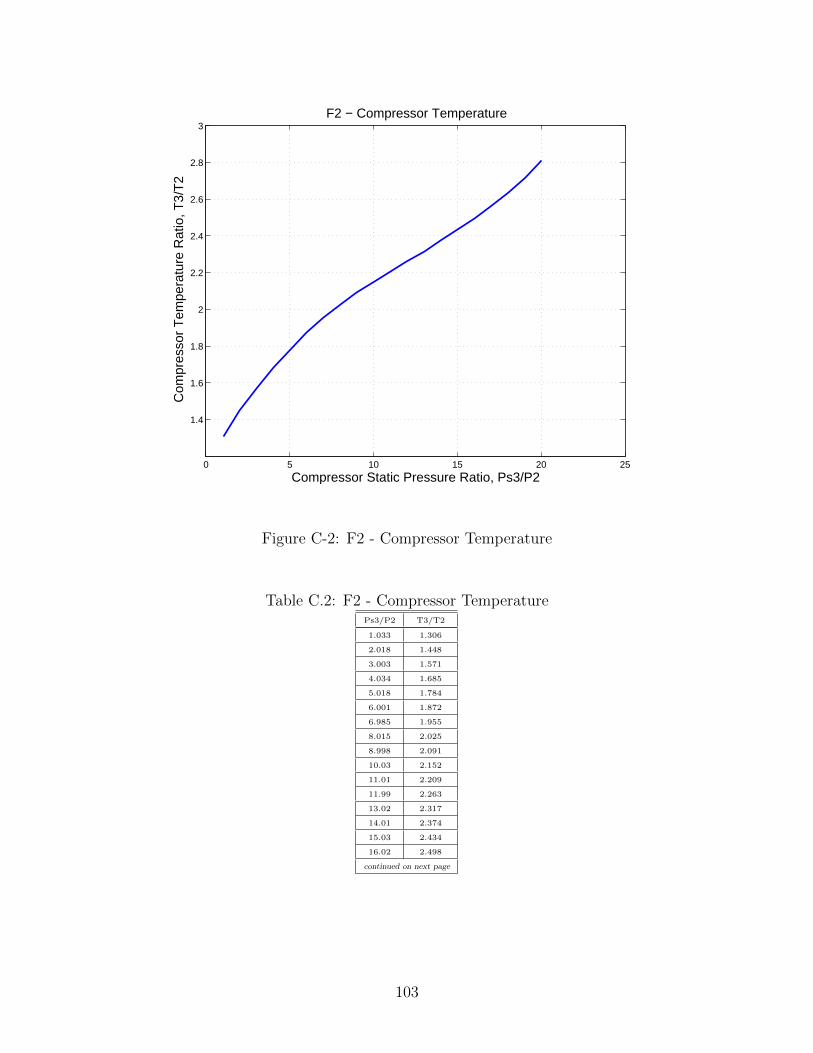
0 5 10 15 20 25
1.4
1.6
1.8
2
2.2
2.4
2.6
2.8
3
Compressor Static Pressure Ratio, Ps3/P2
Com
pres
sor
Tem
pera
ture
Rat
io, T
3/T
2
F2 − Compressor Temperature
Figure C-2: F2 - Compressor Temperature
Table C.2: F2 - Compressor TemperaturePs3/P2 T3/T2
1.033 1.306
2.018 1.448
3.003 1.571
4.034 1.685
5.018 1.784
6.001 1.872
6.985 1.955
8.015 2.025
8.998 2.091
10.03 2.152
11.01 2.209
11.99 2.263
13.02 2.317
14.01 2.374
15.03 2.434
16.02 2.498
continued on next page
103

continued from previous page
Ps3/P2 T3/T2
17 2.561
18.03 2.637
19.06 2.72
20.04 2.808
104
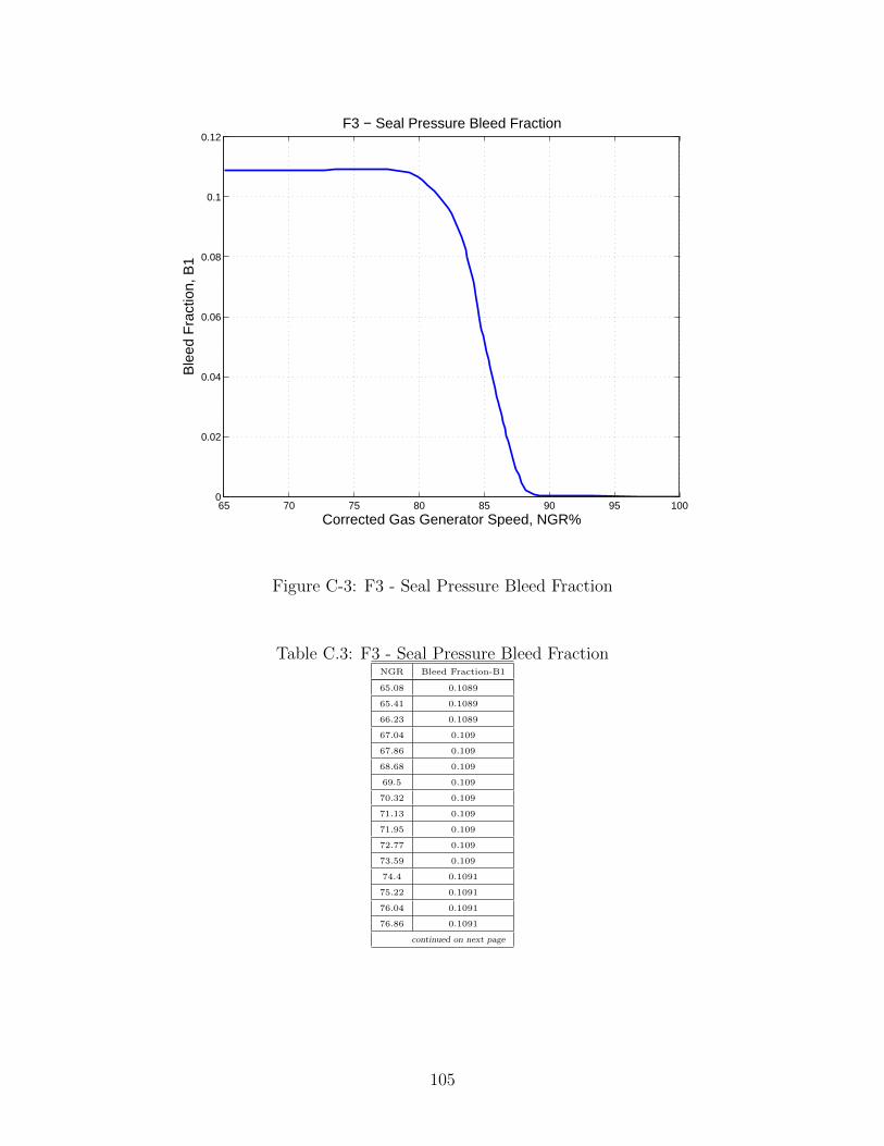
65 70 75 80 85 90 95 1000
0.02
0.04
0.06
0.08
0.1
0.12
Corrected Gas Generator Speed, NGR%
Ble
ed F
ract
ion,
B1
F3 − Seal Pressure Bleed Fraction
Figure C-3: F3 - Seal Pressure Bleed Fraction
Table C.3: F3 - Seal Pressure Bleed FractionNGR Bleed Fraction-B1
65.08 0.1089
65.41 0.1089
66.23 0.1089
67.04 0.109
67.86 0.109
68.68 0.109
69.5 0.109
70.32 0.109
71.13 0.109
71.95 0.109
72.77 0.109
73.59 0.109
74.4 0.1091
75.22 0.1091
76.04 0.1091
76.86 0.1091
continued on next page
105
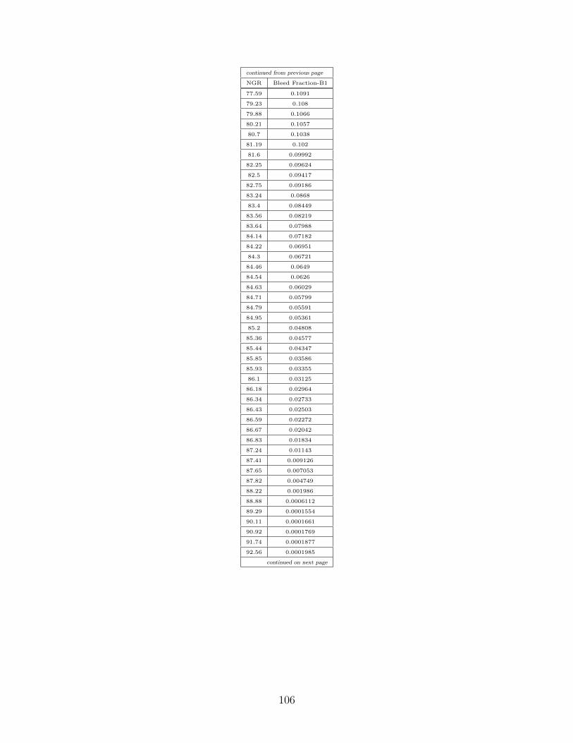
continued from previous page
NGR Bleed Fraction-B1
77.59 0.1091
79.23 0.108
79.88 0.1066
80.21 0.1057
80.7 0.1038
81.19 0.102
81.6 0.09992
82.25 0.09624
82.5 0.09417
82.75 0.09186
83.24 0.0868
83.4 0.08449
83.56 0.08219
83.64 0.07988
84.14 0.07182
84.22 0.06951
84.3 0.06721
84.46 0.0649
84.54 0.0626
84.63 0.06029
84.71 0.05799
84.79 0.05591
84.95 0.05361
85.2 0.04808
85.36 0.04577
85.44 0.04347
85.85 0.03586
85.93 0.03355
86.1 0.03125
86.18 0.02964
86.34 0.02733
86.43 0.02503
86.59 0.02272
86.67 0.02042
86.83 0.01834
87.24 0.01143
87.41 0.009126
87.65 0.007053
87.82 0.004749
88.22 0.001986
88.88 0.0006112
89.29 0.0001554
90.11 0.0001661
90.92 0.0001769
91.74 0.0001877
92.56 0.0001985
continued on next page
106

continued from previous page
NGR Bleed Fraction-B1
93.38 0.0002092
97.06 2.71e-005
97.87 3.79e-005
98.69 4.87e-005
100 6.59e-005
107
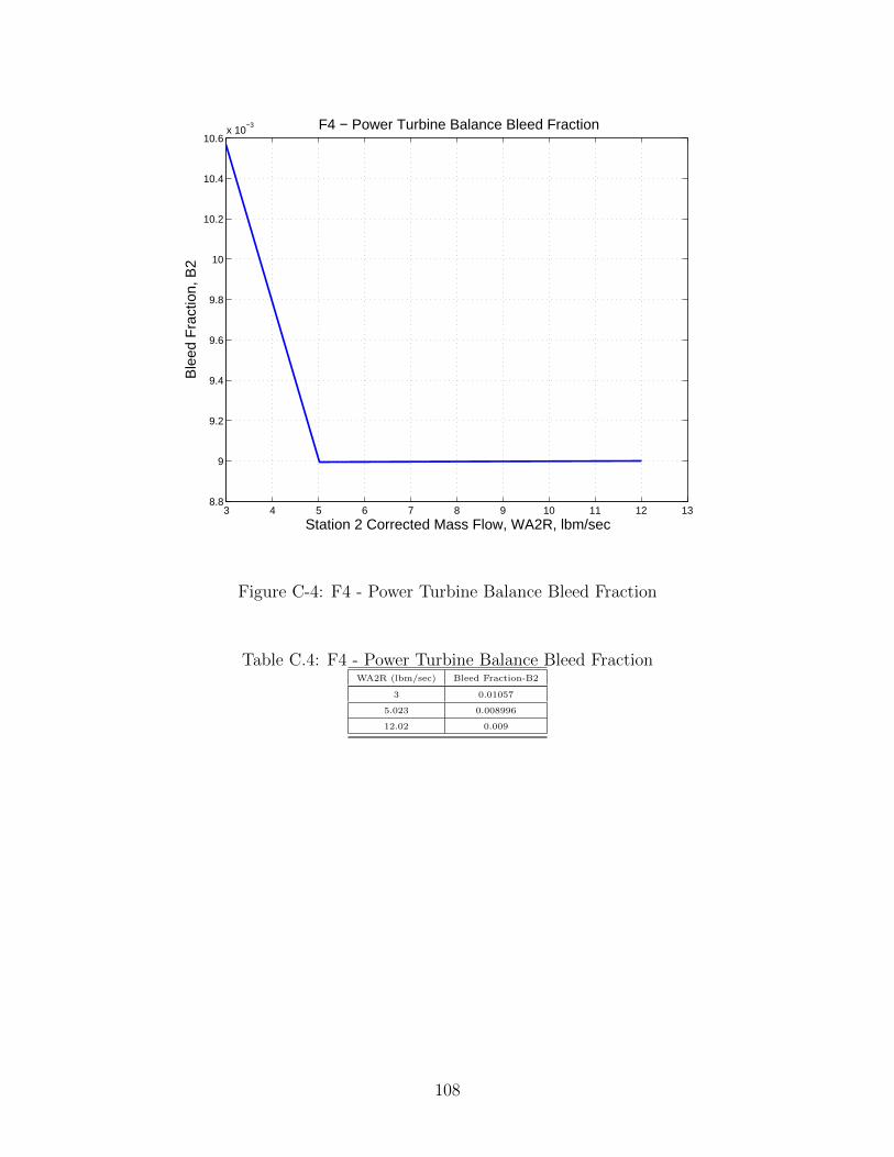
3 4 5 6 7 8 9 10 11 12 138.8
9
9.2
9.4
9.6
9.8
10
10.2
10.4
10.6x 10
−3
Station 2 Corrected Mass Flow, WA2R, lbm/sec
Ble
ed F
ract
ion,
B2
F4 − Power Turbine Balance Bleed Fraction
Figure C-4: F4 - Power Turbine Balance Bleed Fraction
Table C.4: F4 - Power Turbine Balance Bleed FractionWA2R (lbm/sec) Bleed Fraction-B2
3 0.01057
5.023 0.008996
12.02 0.009
108
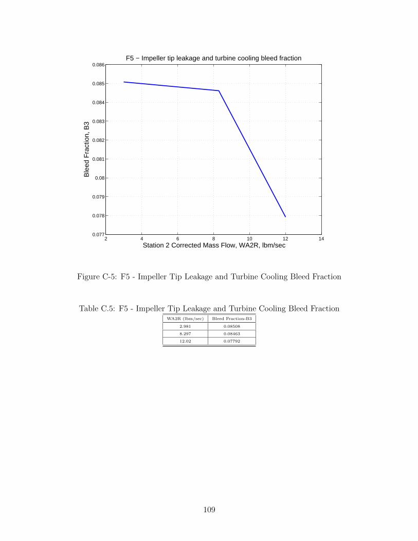
2 4 6 8 10 12 140.077
0.078
0.079
0.08
0.081
0.082
0.083
0.084
0.085
0.086
Station 2 Corrected Mass Flow, WA2R, lbm/sec
Ble
ed F
ract
ion,
B3
F5 − Impeller tip leakage and turbine cooling bleed fraction
Figure C-5: F5 - Impeller Tip Leakage and Turbine Cooling Bleed Fraction
Table C.5: F5 - Impeller Tip Leakage and Turbine Cooling Bleed FractionWA2R (lbm/sec) Bleed Fraction-B3
2.981 0.08508
8.297 0.08463
12.02 0.07792
109
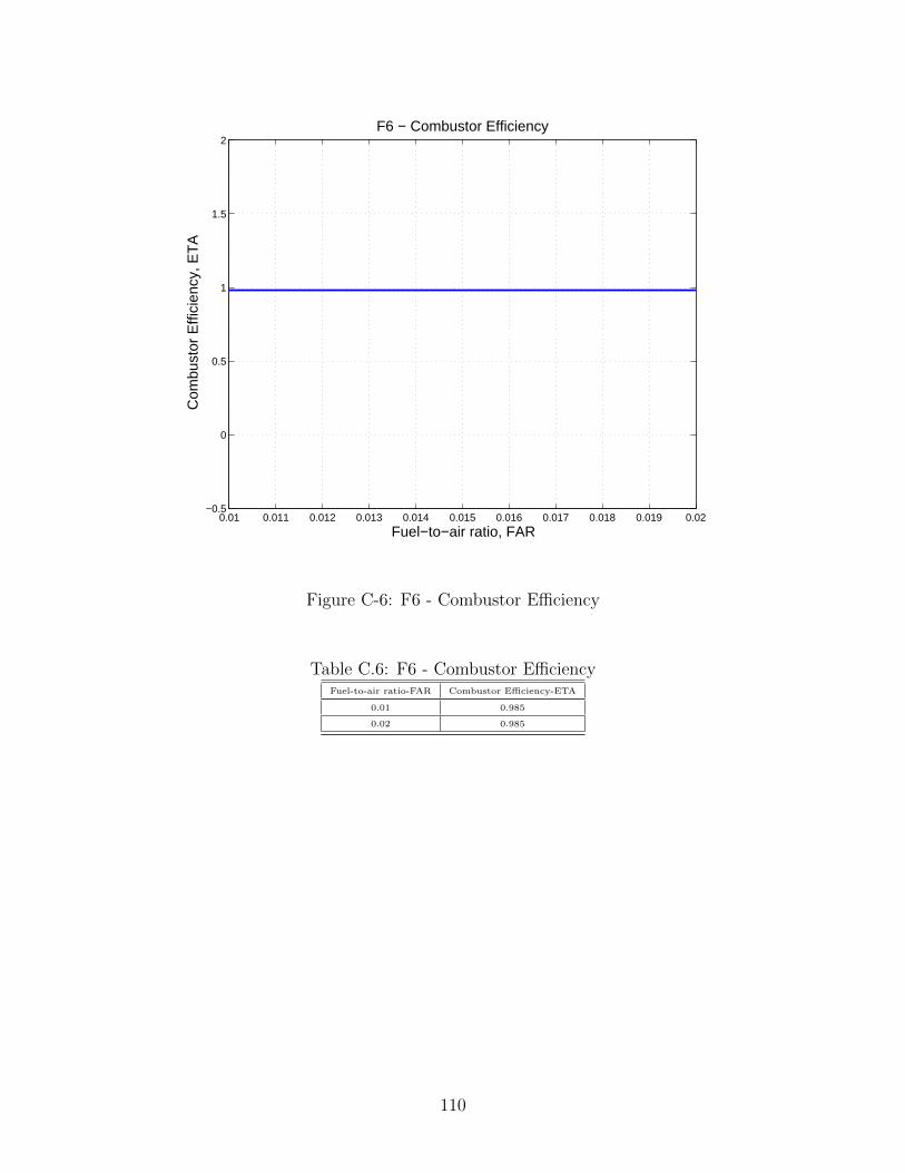
0.01 0.011 0.012 0.013 0.014 0.015 0.016 0.017 0.018 0.019 0.02−0.5
0
0.5
1
1.5
2
Fuel−to−air ratio, FAR
Com
bust
or E
ffici
ency
, ET
A
F6 − Combustor Efficiency
Figure C-6: F6 - Combustor Efficiency
Table C.6: F6 - Combustor EfficiencyFuel-to-air ratio-FAR Combustor Efficiency-ETA
0.01 0.985
0.02 0.985
110
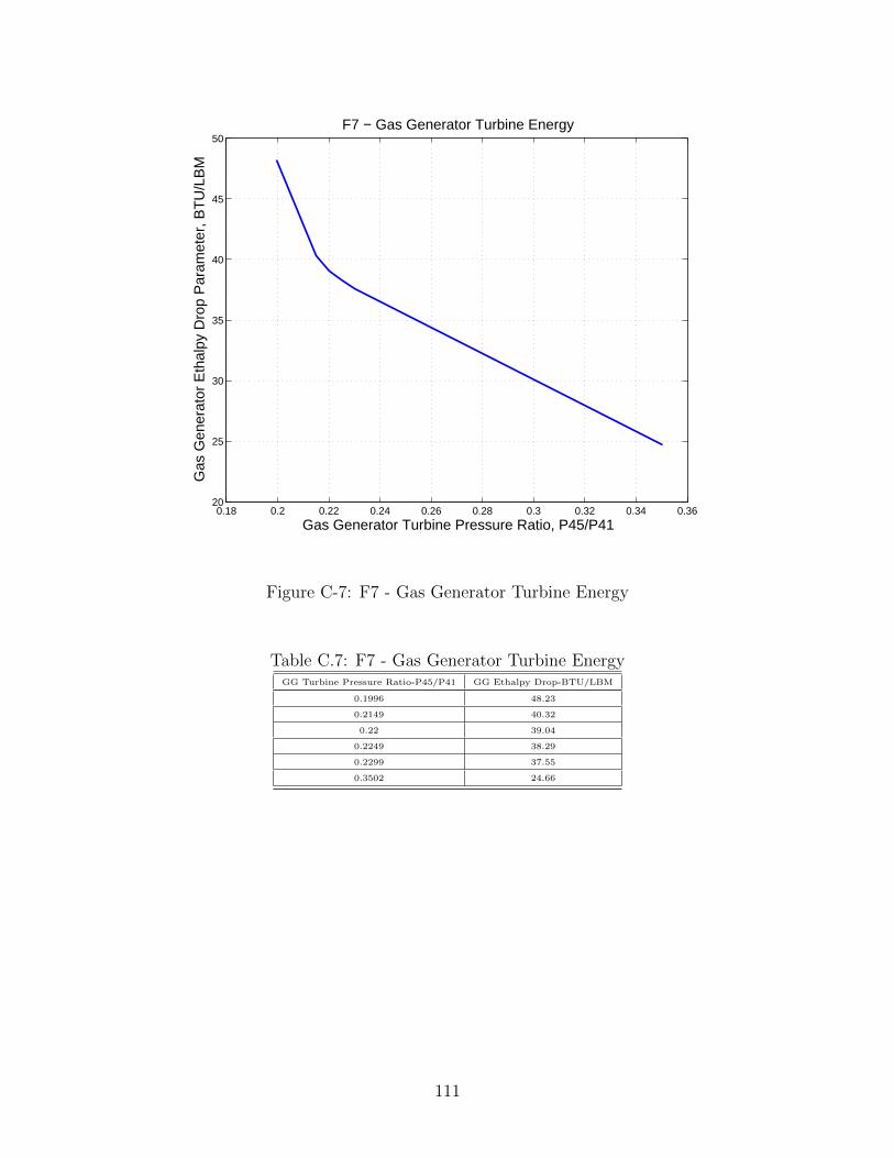
0.18 0.2 0.22 0.24 0.26 0.28 0.3 0.32 0.34 0.3620
25
30
35
40
45
50
Gas Generator Turbine Pressure Ratio, P45/P41
Gas
Gen
erat
or E
thal
py D
rop
Par
amet
er, B
TU
/LB
M
F7 − Gas Generator Turbine Energy
Figure C-7: F7 - Gas Generator Turbine Energy
Table C.7: F7 - Gas Generator Turbine EnergyGG Turbine Pressure Ratio-P45/P41 GG Ethalpy Drop-BTU/LBM
0.1996 48.23
0.2149 40.32
0.22 39.04
0.2249 38.29
0.2299 37.55
0.3502 24.66
111
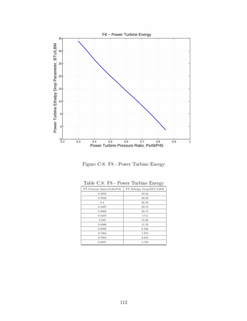
0.2 0.3 0.4 0.5 0.6 0.7 0.8 0.9 1−5
0
5
10
15
20
25
30
35
Power Turbine Pressure Ratio, Ps49/P45
Pow
er T
urbi
ne E
thal
py D
rop
Par
amet
er, B
TU
/LB
M
F8 − Power Turbine Energy
Figure C-8: F8 - Power Turbine Energy
Table C.8: F8 - Power Turbine EnergyPT Pressure Ratio-Ps49/P45 PT Ethalpy Drop-BTU/LBM
0.2993 33.94
0.3503 30.33
0.4 26.58
0.4497 23.13
0.4982 20.13
0.5493 17.2
0.599 14.28
0.6488 11.35
0.6999 8.348
0.7484 5.272
0.7994 2.045
0.8491 -1.331
112
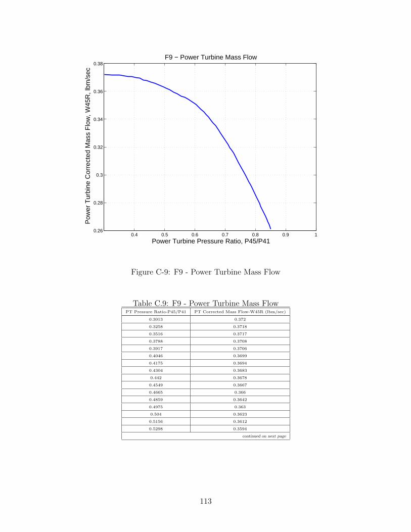
0.4 0.5 0.6 0.7 0.8 0.9 10.26
0.28
0.3
0.32
0.34
0.36
0.38
Power Turbine Pressure Ratio, P45/P41
Pow
er T
urbi
ne C
orre
cted
Mas
s F
low
, W45
R, l
bm/s
ec
F9 − Power Turbine Mass Flow
Figure C-9: F9 - Power Turbine Mass Flow
Table C.9: F9 - Power Turbine Mass FlowPT Pressure Ratio-P45/P41 PT Corrected Mass Flow-W45R (lbm/sec)
0.3013 0.372
0.3258 0.3718
0.3516 0.3717
0.3788 0.3708
0.3917 0.3706
0.4046 0.3699
0.4175 0.3694
0.4304 0.3683
0.442 0.3678
0.4549 0.3667
0.4665 0.366
0.4859 0.3642
0.4975 0.363
0.504 0.3623
0.5156 0.3612
0.5298 0.3594
continued on next page
113
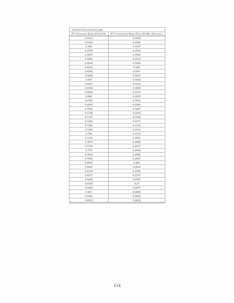
continued from previous page
PT Pressure Ratio-P45/P41 PT Corrected Mass Flow-W45R (lbm/sec)
0.5414 0.3582
0.5543 0.3566
0.566 0.3557
0.5789 0.3543
0.5879 0.3529
0.5982 0.3513
0.6034 0.3506
0.6124 0.349
0.6202 0.3471
0.6292 0.3453
0.637 0.3434
0.6447 0.3416
0.6538 0.3393
0.6602 0.3374
0.668 0.3353
0.6783 0.3323
0.6835 0.3302
0.7041 0.3237
0.7106 0.3216
0.7157 0.3195
0.7222 0.3177
0.7286 0.3154
0.7338 0.3133
0.739 0.3112
0.7441 0.3091
0.7674 0.2998
0.7725 0.2977
0.779 0.2949
0.7842 0.2928
0.7893 0.2907
0.8035 0.284
0.8087 0.2819
0.8138 0.2796
0.8177 0.2775
0.8293 0.2721
0.8345 0.27
0.8384 0.2677
0.841 0.2666
0.8461 0.2645
0.8513 0.2612
114
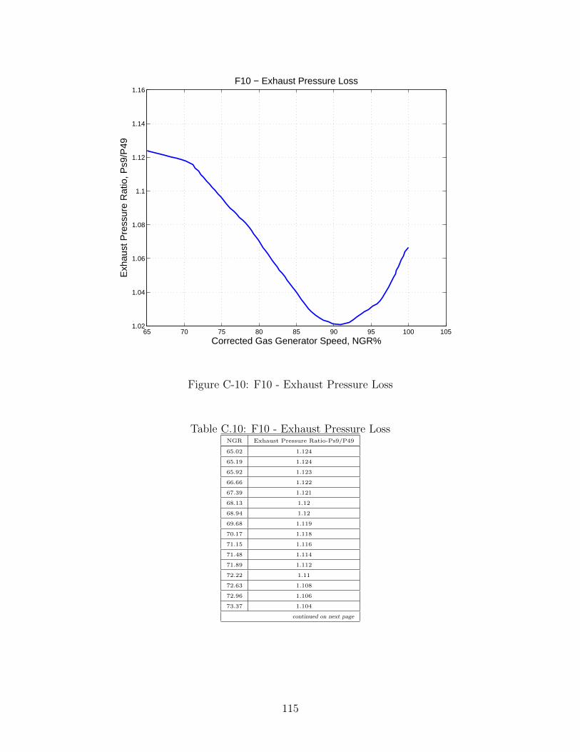
65 70 75 80 85 90 95 100 1051.02
1.04
1.06
1.08
1.1
1.12
1.14
1.16
Corrected Gas Generator Speed, NGR%
Exh
aust
Pre
ssur
e R
atio
, Ps9
/P49
F10 − Exhaust Pressure Loss
Figure C-10: F10 - Exhaust Pressure Loss
Table C.10: F10 - Exhaust Pressure LossNGR Exhaust Pressure Ratio-Ps9/P49
65.02 1.124
65.19 1.124
65.92 1.123
66.66 1.122
67.39 1.121
68.13 1.12
68.94 1.12
69.68 1.119
70.17 1.118
71.15 1.116
71.48 1.114
71.89 1.112
72.22 1.11
72.63 1.108
72.96 1.106
73.37 1.104
continued on next page
115
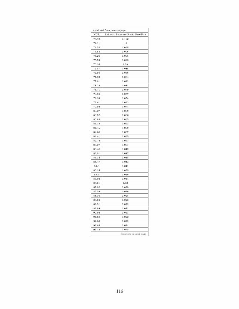
continued from previous page
NGR Exhaust Pressure Ratio-Ps9/P49
73.78 1.102
74.11 1.1
74.52 1.098
74.85 1.096
75.26 1.095
75.59 1.093
76.16 1.09
76.57 1.088
76.98 1.086
77.39 1.084
77.81 1.082
78.22 1.081
78.71 1.079
78.96 1.077
79.28 1.074
79.61 1.073
79.94 1.071
80.27 1.069
80.52 1.066
80.85 1.065
81.18 1.063
81.75 1.059
82.08 1.057
82.41 1.055
82.74 1.053
83.07 1.051
83.48 1.049
83.81 1.047
84.14 1.045
84.47 1.043
84.8 1.041
85.13 1.039
85.7 1.036
86.03 1.034
86.61 1.03
87.02 1.028
87.59 1.026
88.16 1.025
88.66 1.023
89.31 1.022
89.88 1.021
90.94 1.021
91.68 1.022
92.08 1.022
92.65 1.024
93.14 1.025
continued on next page
116
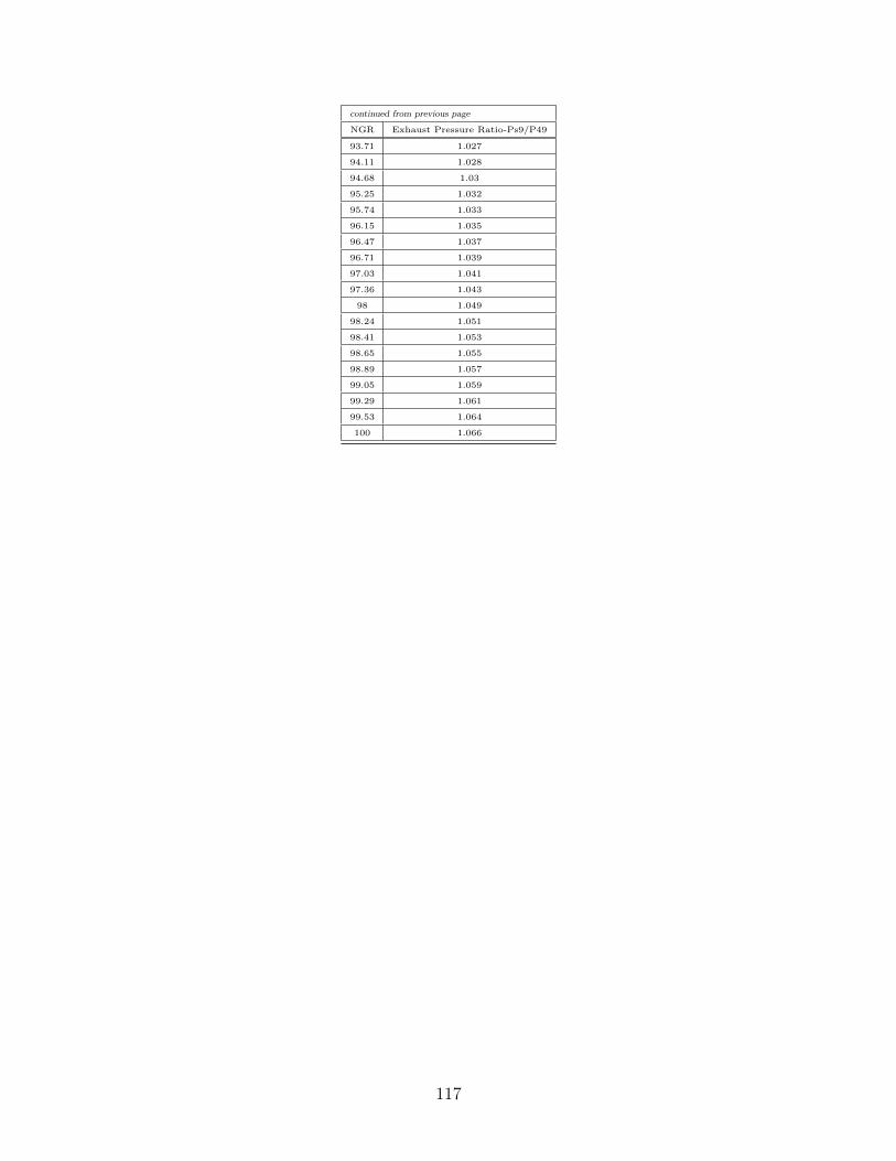
continued from previous page
NGR Exhaust Pressure Ratio-Ps9/P49
93.71 1.027
94.11 1.028
94.68 1.03
95.25 1.032
95.74 1.033
96.15 1.035
96.47 1.037
96.71 1.039
97.03 1.041
97.36 1.043
98 1.049
98.24 1.051
98.41 1.053
98.65 1.055
98.89 1.057
99.05 1.059
99.29 1.061
99.53 1.064
100 1.066
117
Appendix D
Fuel Control Model Diagrams
118
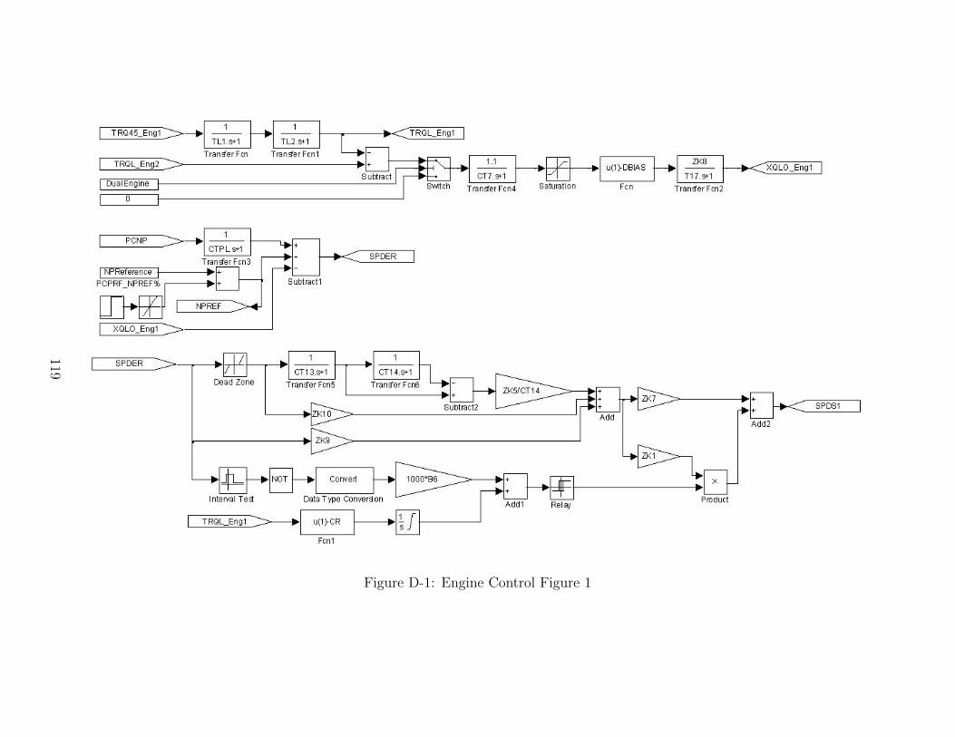
Figure D-1: Engine Control Figure 1
119
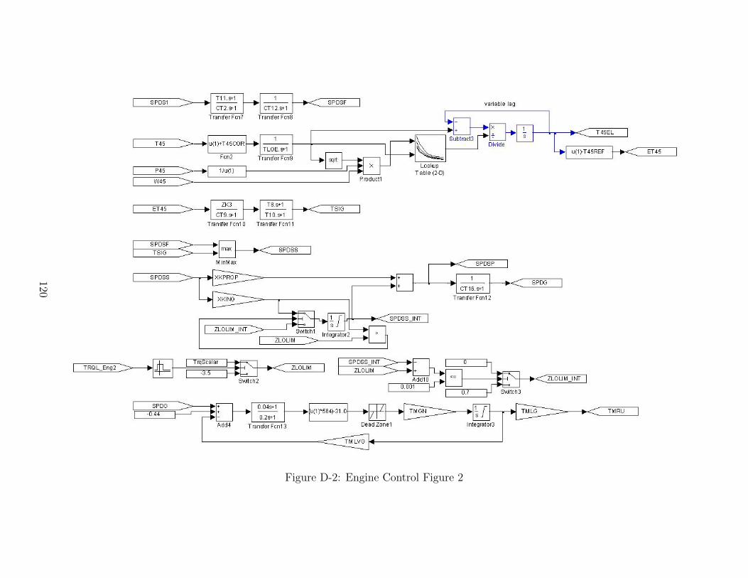
Figure D-2: Engine Control Figure 2
120
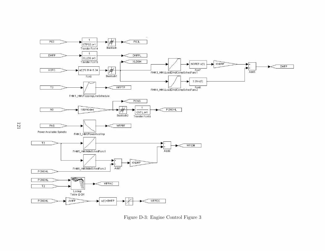
Figure D-3: Engine Control Figure 3
121
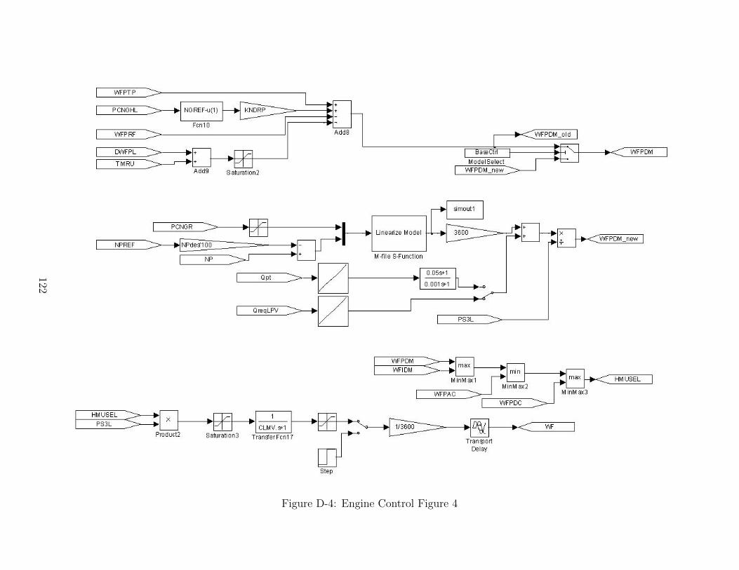
Figure D-4: Engine Control Figure 4
122
Appendix E
Fuel Control Constants
See the Model Variable Table 1 in the nomenclature section.
123
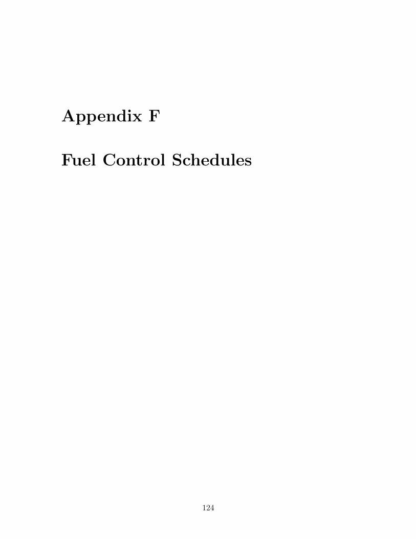
Appendix F
Fuel Control Schedules
124
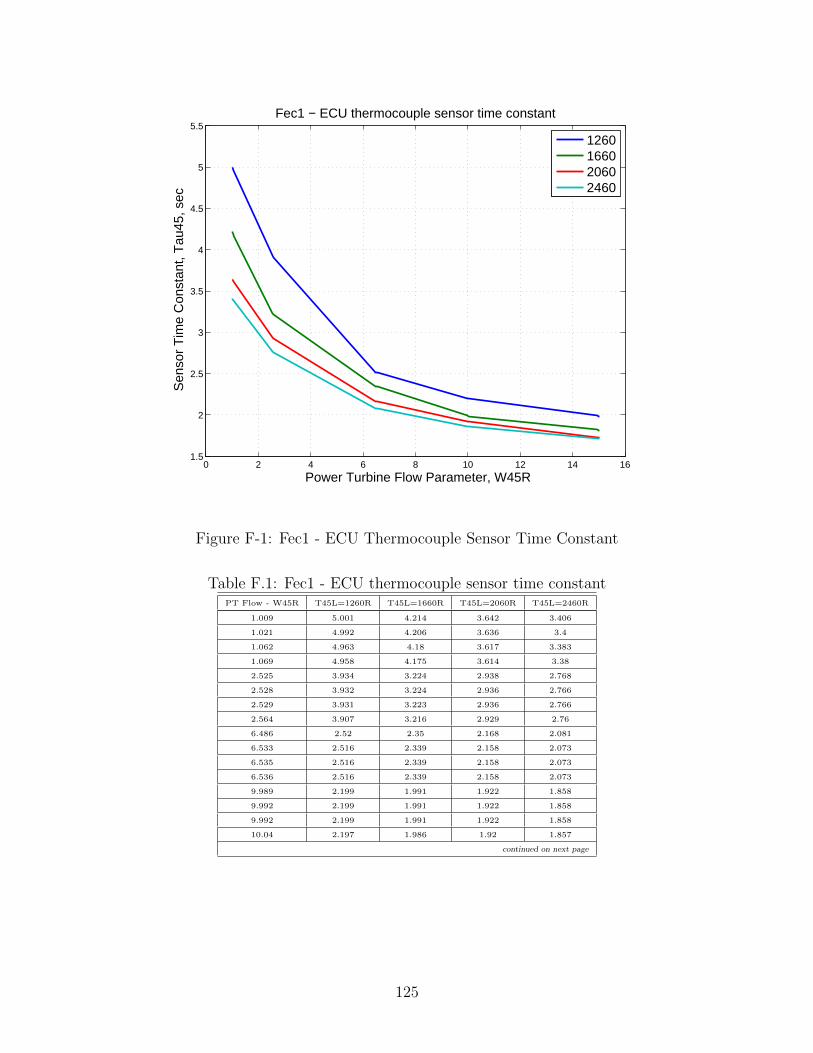
0 2 4 6 8 10 12 14 161.5
2
2.5
3
3.5
4
4.5
5
5.5
Power Turbine Flow Parameter, W45R
Sen
sor
Tim
e C
onst
ant,
Tau
45, s
ec
Fec1 − ECU thermocouple sensor time constant
1260166020602460
Figure F-1: Fec1 - ECU Thermocouple Sensor Time Constant
Table F.1: Fec1 - ECU thermocouple sensor time constantPT Flow - W45R T45L=1260R T45L=1660R T45L=2060R T45L=2460R
1.009 5.001 4.214 3.642 3.406
1.021 4.992 4.206 3.636 3.4
1.062 4.963 4.18 3.617 3.383
1.069 4.958 4.175 3.614 3.38
2.525 3.934 3.224 2.938 2.768
2.528 3.932 3.224 2.936 2.766
2.529 3.931 3.223 2.936 2.766
2.564 3.907 3.216 2.929 2.76
6.486 2.52 2.35 2.168 2.081
6.533 2.516 2.339 2.158 2.073
6.535 2.516 2.339 2.158 2.073
6.536 2.516 2.339 2.158 2.073
9.989 2.199 1.991 1.922 1.858
9.992 2.199 1.991 1.922 1.858
9.992 2.199 1.991 1.922 1.858
10.04 2.197 1.986 1.92 1.857
continued on next page
125

continued from previous page
PT Flow - W45R T45L=1260R T45L=1660R T45L=2060R T45L=2460R
14.95 1.989 1.82 1.726 1.714
14.99 1.987 1.818 1.724 1.713
15.04 1.985 1.817 1.722 1.712
15.04 1.985 1.817 1.722 1.712
126
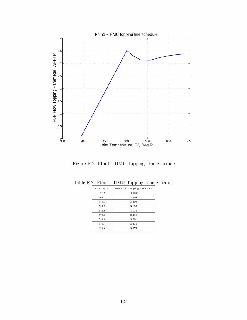
350 400 450 500 550 600 6500
0.5
1
1.5
2
2.5
3
3.5
4
Inlet Temperature, T2, Deg R
Fue
l Flo
w T
oppi
ng P
aram
eter
, WF
PT
P
Fhm1 − HMU topping line schedule
Figure F-2: Fhm1 - HMU Topping Line Schedule
Table F.2: Fhm1 - HMU Topping Line ScheduleT2 (Deg R) Fuel Flow Topping - WFPTP
393.9 0.09091
501.2 3.509
515.3 3.309
534.3 3.136
554.9 3.118
575.6 3.218
594.8 3.291
615.4 3.336
634.6 3.373
127
20 30 40 50 60 70 80 90 100 110 1200
2
4
6
8
10
12
Power Available Spindle Angle, deg
Fue
l Flo
w P
ower
Ava
ilabl
e P
aram
eter
, WF
PR
F
Fhm2 − HMU Power Available input schedule
Figure F-3: Fhm2 - HMU Power Available Input Schedule
Table F.3: Fhm2 - HMU Power Available Input SchedulePower Available Spindle Fuel Flow Reference - WFPRF
28.62 10.4
30.07 9.836
39.91 7.022
50.21 5.736
59.92 4.844
70.21 3.812
79.93 2.808
89.65 1.945
99.92 1.224
109.9 0.7857
119.9 0.03619
128
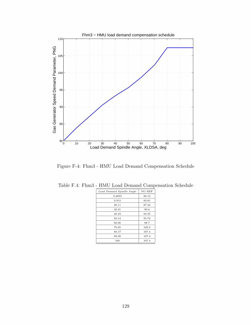
0 10 20 30 40 50 60 70 80 90 10080
85
90
95
100
105
110
Load Demand Spindle Angle, XLDSA, deg
Gas
Gen
erat
or S
peed
Dem
and
Par
amet
er, P
NG
Fhm3 − HMU load demand compensation schedule
Figure F-4: Fhm3 - HMU Load Demand Compensation Schedule
Table F.4: Fhm3 - HMU Load Demand Compensation ScheduleLoad Demand Spindle Angle NG REF
0.2833 80.15
9.915 83.81
20.11 87.24
30.31 90.6
40.23 93.35
50.14 95.72
60.06 98.7
70.25 102.3
80.17 107.4
90.08 107.4
100 107.4
129
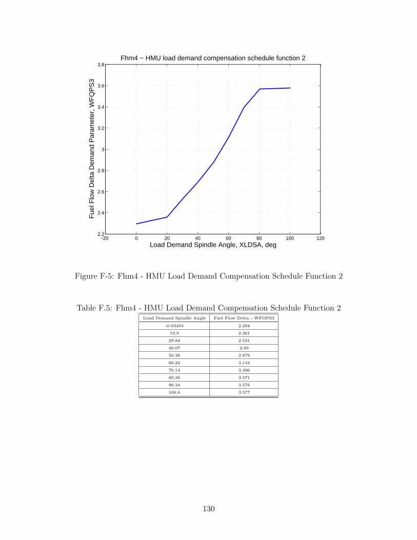
−20 0 20 40 60 80 100 1202.2
2.4
2.6
2.8
3
3.2
3.4
3.6
3.8
Load Demand Spindle Angle, XLDSA, deg
Fue
l Flo
w D
elta
Dem
and
Par
amet
er, W
FQ
PS
3
Fhm4 − HMU load demand compensation schedule function 2
Figure F-5: Fhm4 - HMU Load Demand Compensation Schedule Function 2
Table F.5: Fhm4 - HMU Load Demand Compensation Schedule Function 2Load Demand Spindle Angle Fuel Flow Delta - WFOPS3
-0.03453 2.294
19.9 2.361
29.84 2.531
40.07 2.69
50.29 2.879
60.22 3.119
70.14 3.396
80.36 3.571
90.34 3.576
100.6 3.577
130
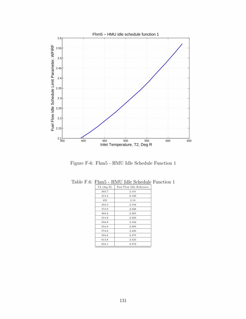
350 400 450 500 550 600 6502.1
2.15
2.2
2.25
2.3
2.35
2.4
2.45
2.5
2.55
2.6
Inlet Temperature, T2, Deg R
Fue
l Flo
w Id
le S
ched
ule
Lim
it P
aram
eter
, WF
IRF
Fhm5 − HMU idle schedule function 1
Figure F-6: Fhm5 - HMU Idle Schedule Function 1
Table F.6: Fhm5 - HMU Idle Schedule Function 1T2 (deg R) Fuel Flow Idle Reference
393.7 2.101
414.4 2.129
435 2.16
454.3 2.194
474.9 2.228
494.2 2.265
514.8 2.303
534.8 2.342
554.8 2.385
574.8 2.429
594.8 2.475
614.8 2.523
634.1 2.572
131
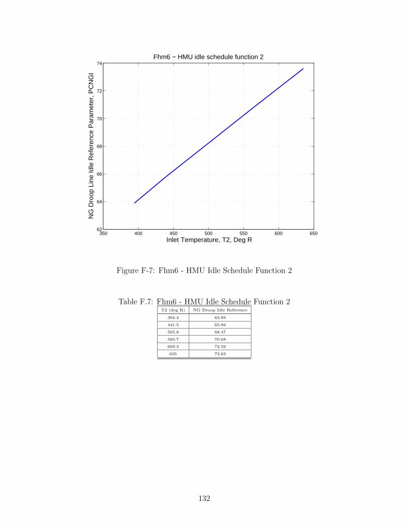
350 400 450 500 550 600 65062
64
66
68
70
72
74
Inlet Temperature, T2, Deg R
NG
Dro
op L
ine
Idle
Ref
eren
ce P
aram
eter
, PC
NG
I
Fhm6 − HMU idle schedule function 2
Figure F-7: Fhm6 - HMU Idle Schedule Function 2
Table F.7: Fhm6 - HMU Idle Schedule Function 2T2 (deg R) NG Droop Idle Reference
394.4 63.89
441.5 65.89
505.8 68.47
560.7 70.68
609.3 72.59
635 73.63
132
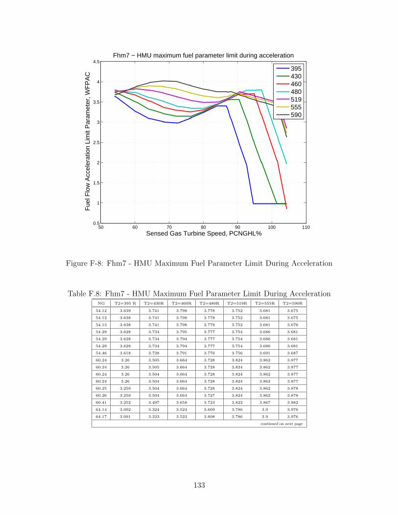
50 60 70 80 90 100 1100.5
1
1.5
2
2.5
3
3.5
4
4.5
Sensed Gas Turbine Speed, PCNGHL%
Fue
l Flo
w A
ccel
erat
ion
Lim
it P
aram
eter
, WF
PA
C
Fhm7 − HMU maximum fuel parameter limit during acceleration
395430460480519555590
Figure F-8: Fhm7 - HMU Maximum Fuel Parameter Limit During Acceleration
Table F.8: Fhm7 - HMU Maximum Fuel Parameter Limit During AccelerationNG T2=395 R T2=430R T2=460R T2=480R T2=519R T2=555R T2=590R
54.12 3.639 3.741 3.798 3.778 3.752 3.681 3.675
54.12 3.638 3.741 3.798 3.778 3.752 3.681 3.675
54.13 3.638 3.741 3.798 3.778 3.752 3.681 3.676
54.29 3.628 3.734 3.795 3.777 3.754 3.686 3.681
54.29 3.628 3.734 3.794 3.777 3.754 3.686 3.681
54.29 3.628 3.734 3.794 3.777 3.754 3.686 3.681
54.46 3.618 3.728 3.791 3.776 3.756 3.691 3.687
60.24 3.26 3.505 3.664 3.728 3.824 3.862 3.877
60.24 3.26 3.505 3.664 3.728 3.824 3.862 3.877
60.24 3.26 3.504 3.664 3.728 3.824 3.862 3.877
60.24 3.26 3.504 3.664 3.728 3.824 3.862 3.877
60.25 3.259 3.504 3.664 3.728 3.824 3.862 3.878
60.26 3.259 3.504 3.664 3.727 3.824 3.862 3.878
60.41 3.252 3.497 3.658 3.723 3.822 3.867 3.882
64.14 3.092 3.324 3.524 3.609 3.786 3.9 3.976
64.17 3.091 3.323 3.523 3.608 3.786 3.9 3.976
continued on next page
133
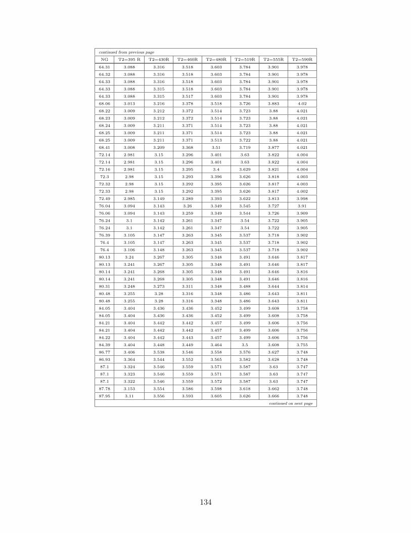
continued from previous page
NG T2=395 R T2=430R T2=460R T2=480R T2=519R T2=555R T2=590R
64.31 3.088 3.316 3.518 3.603 3.784 3.901 3.978
64.32 3.088 3.316 3.518 3.603 3.784 3.901 3.978
64.33 3.088 3.316 3.518 3.603 3.784 3.901 3.978
64.33 3.088 3.315 3.518 3.603 3.784 3.901 3.978
64.33 3.088 3.315 3.517 3.603 3.784 3.901 3.978
68.06 3.013 3.216 3.378 3.518 3.726 3.883 4.02
68.22 3.009 3.212 3.372 3.514 3.723 3.88 4.021
68.23 3.009 3.212 3.372 3.514 3.723 3.88 4.021
68.24 3.009 3.211 3.371 3.514 3.723 3.88 4.021
68.25 3.009 3.211 3.371 3.514 3.723 3.88 4.021
68.25 3.009 3.211 3.371 3.513 3.722 3.88 4.021
68.41 3.008 3.209 3.368 3.51 3.719 3.877 4.021
72.14 2.981 3.15 3.296 3.401 3.63 3.822 4.004
72.14 2.981 3.15 3.296 3.401 3.63 3.822 4.004
72.16 2.981 3.15 3.295 3.4 3.629 3.821 4.004
72.3 2.98 3.15 3.293 3.396 3.626 3.818 4.003
72.32 2.98 3.15 3.292 3.395 3.626 3.817 4.003
72.33 2.98 3.15 3.292 3.395 3.626 3.817 4.002
72.49 2.985 3.149 3.289 3.393 3.622 3.813 3.998
76.04 3.094 3.143 3.26 3.349 3.545 3.727 3.91
76.06 3.094 3.143 3.259 3.349 3.544 3.726 3.909
76.24 3.1 3.142 3.261 3.347 3.54 3.722 3.905
76.24 3.1 3.142 3.261 3.347 3.54 3.722 3.905
76.39 3.105 3.147 3.263 3.345 3.537 3.718 3.902
76.4 3.105 3.147 3.263 3.345 3.537 3.718 3.902
76.4 3.106 3.148 3.263 3.345 3.537 3.718 3.902
80.13 3.24 3.267 3.305 3.348 3.491 3.646 3.817
80.13 3.241 3.267 3.305 3.348 3.491 3.646 3.817
80.14 3.241 3.268 3.305 3.348 3.491 3.646 3.816
80.14 3.241 3.268 3.305 3.348 3.491 3.646 3.816
80.31 3.248 3.273 3.311 3.348 3.488 3.644 3.814
80.48 3.255 3.28 3.316 3.348 3.486 3.643 3.811
80.48 3.255 3.28 3.316 3.348 3.486 3.643 3.811
84.05 3.404 3.436 3.436 3.452 3.499 3.608 3.758
84.05 3.404 3.436 3.436 3.452 3.499 3.608 3.758
84.21 3.404 3.442 3.442 3.457 3.499 3.606 3.756
84.21 3.404 3.442 3.442 3.457 3.499 3.606 3.756
84.22 3.404 3.442 3.443 3.457 3.499 3.606 3.756
84.39 3.404 3.448 3.449 3.464 3.5 3.608 3.755
86.77 3.406 3.538 3.546 3.558 3.576 3.627 3.748
86.93 3.364 3.544 3.552 3.565 3.582 3.628 3.748
87.1 3.324 3.546 3.559 3.571 3.587 3.63 3.747
87.1 3.323 3.546 3.559 3.571 3.587 3.63 3.747
87.1 3.322 3.546 3.559 3.572 3.587 3.63 3.747
87.78 3.153 3.554 3.586 3.598 3.618 3.662 3.748
87.95 3.11 3.556 3.593 3.605 3.626 3.666 3.748
continued on next page
134
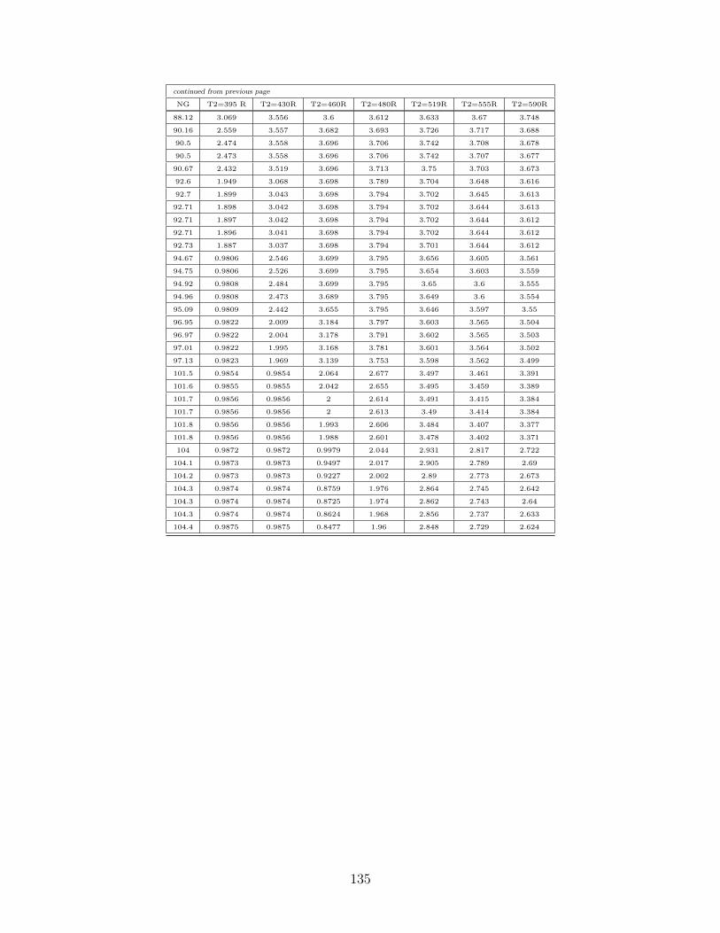
continued from previous page
NG T2=395 R T2=430R T2=460R T2=480R T2=519R T2=555R T2=590R
88.12 3.069 3.556 3.6 3.612 3.633 3.67 3.748
90.16 2.559 3.557 3.682 3.693 3.726 3.717 3.688
90.5 2.474 3.558 3.696 3.706 3.742 3.708 3.678
90.5 2.473 3.558 3.696 3.706 3.742 3.707 3.677
90.67 2.432 3.519 3.696 3.713 3.75 3.703 3.673
92.6 1.949 3.068 3.698 3.789 3.704 3.648 3.616
92.7 1.899 3.043 3.698 3.794 3.702 3.645 3.613
92.71 1.898 3.042 3.698 3.794 3.702 3.644 3.613
92.71 1.897 3.042 3.698 3.794 3.702 3.644 3.612
92.71 1.896 3.041 3.698 3.794 3.702 3.644 3.612
92.73 1.887 3.037 3.698 3.794 3.701 3.644 3.612
94.67 0.9806 2.546 3.699 3.795 3.656 3.605 3.561
94.75 0.9806 2.526 3.699 3.795 3.654 3.603 3.559
94.92 0.9808 2.484 3.699 3.795 3.65 3.6 3.555
94.96 0.9808 2.473 3.689 3.795 3.649 3.6 3.554
95.09 0.9809 2.442 3.655 3.795 3.646 3.597 3.55
96.95 0.9822 2.009 3.184 3.797 3.603 3.565 3.504
96.97 0.9822 2.004 3.178 3.791 3.602 3.565 3.503
97.01 0.9822 1.995 3.168 3.781 3.601 3.564 3.502
97.13 0.9823 1.969 3.139 3.753 3.598 3.562 3.499
101.5 0.9854 0.9854 2.064 2.677 3.497 3.461 3.391
101.6 0.9855 0.9855 2.042 2.655 3.495 3.459 3.389
101.7 0.9856 0.9856 2 2.614 3.491 3.415 3.384
101.7 0.9856 0.9856 2 2.613 3.49 3.414 3.384
101.8 0.9856 0.9856 1.993 2.606 3.484 3.407 3.377
101.8 0.9856 0.9856 1.988 2.601 3.478 3.402 3.371
104 0.9872 0.9872 0.9979 2.044 2.931 2.817 2.722
104.1 0.9873 0.9873 0.9497 2.017 2.905 2.789 2.69
104.2 0.9873 0.9873 0.9227 2.002 2.89 2.773 2.673
104.3 0.9874 0.9874 0.8759 1.976 2.864 2.745 2.642
104.3 0.9874 0.9874 0.8725 1.974 2.862 2.743 2.64
104.3 0.9874 0.9874 0.8624 1.968 2.856 2.737 2.633
104.4 0.9875 0.9875 0.8477 1.96 2.848 2.729 2.624
135
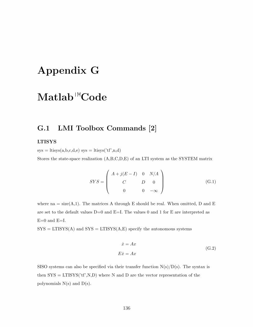
Appendix G
Matlab�Code
G.1 LMI Toolbox Commands [2]
LTISYS
sys = ltisys(a,b,c,d,e) sys = ltisys(’tf’,n,d)
Stores the state-space realization (A,B,C,D,E) of an LTI system as the SYSTEM matrix
SY S =
A+ j(E − I) 0 N/A
C D 0
0 0 −∞
(G.1)
where na = size(A,1). The matrices A through E should be real. When omitted, D and E
are set to the default values D=0 and E=I. The values 0 and 1 for E are interpreted as
E=0 and E=I.
SYS = LTISYS(A) and SYS = LTISYS(A,E) specify the autonomous systems
x = Ax
Ex = Ax(G.2)
SISO systems can also be specified via their transfer function N(s)/D(s). The syntax is
then SYS = LTISYS(’tf’,N,D) where N and D are the vector representation of the
polynomials N(s) and D(s).
136
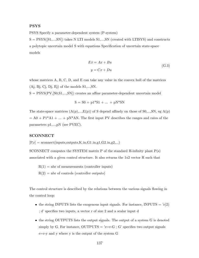
PSYS
PSYS Specify a parameter-dependent system (P-system)
S = PSYS([S1,...,SN]) takes N LTI models S1,...,SN (created with LTISYS) and constructs
a polytopic uncertain model S with equations Specification of uncertain state-space
models
Ex = Ax+Bu
y = Cx+Du(G.3)
whose matrices A, B, C, D, and E can take any value in the convex hull of the matrices
(Aj, Bj, Cj, Dj, Ej) of the models S1,...,SN.
S = PSYS(PV,[S0,S1,...,SN]) creates an affine parameter-dependent uncertain model
S = S0 + p1*S1 + ... + pN*SN
The state-space matrices (A(p),...,E(p)) of S depend affinely on those of S0,...,SN, eg A(p)
= A0 + P1*A1 + ... + pN*AN. The first input PV describes the ranges and rates of the
parameters p1,...,pN (see PVEC).
SCONNECT
[P,r] = sconnect(inputs,outputs,K in,G1 in,g1,G2 in,g2,...)
SCONNECT computes the SYSTEM matrix P of the standard H-infinity plant P(s)
associated with a given control structure. It also returns the 1x2 vector R such that
R(1) = nbr of measurements (controller inputs)
R(2) = nbr of controls (controller outputs)
The control structure is described by the relations between the various signals flowing in
the control loop:
� the string INPUTS lists the exogenous input signals. For instance, INPUTS = ’r(2)
; d’ specifies two inputs, a vector r of size 2 and a scalar input d
� the string OUTPUTS lists the output signals. The output of a system G is denoted
simply by G. For instance, OUTPUTS = ’e=r-G ; G’ specifies two output signals
e=r-y and y where y is the output of the system G
137
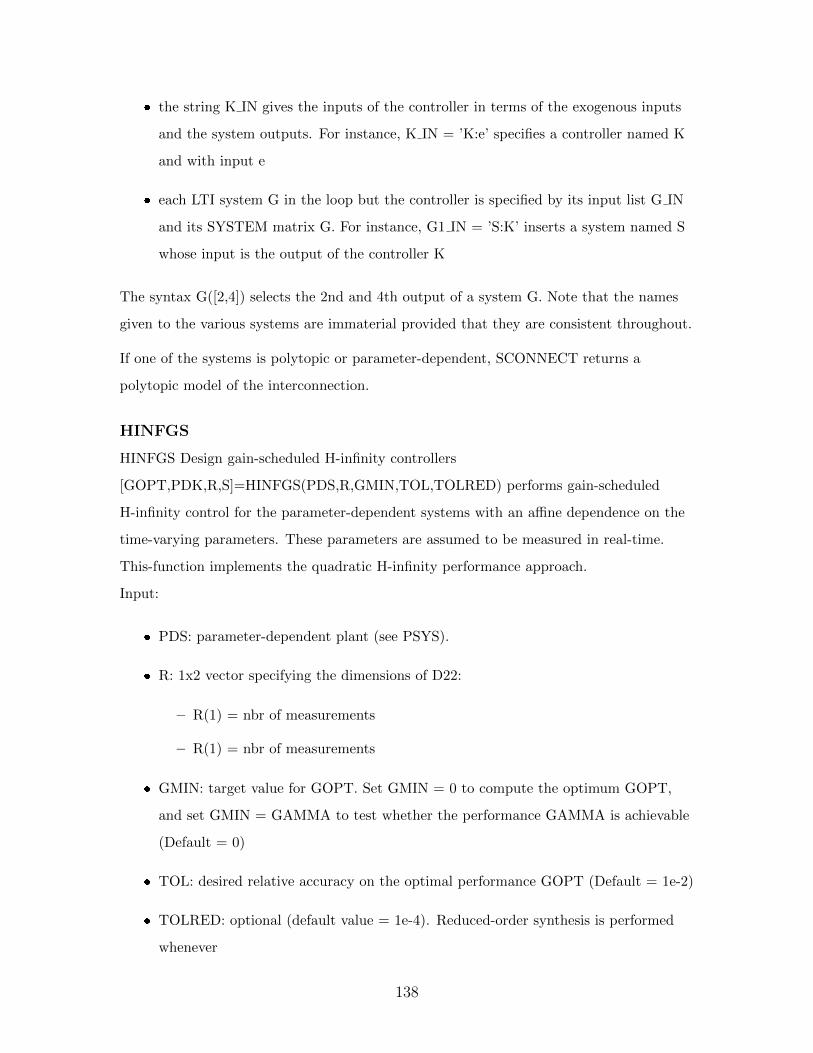
� the string K IN gives the inputs of the controller in terms of the exogenous inputs
and the system outputs. For instance, K IN = ’K:e’ specifies a controller named K
and with input e
� each LTI system G in the loop but the controller is specified by its input list G IN
and its SYSTEM matrix G. For instance, G1 IN = ’S:K’ inserts a system named S
whose input is the output of the controller K
The syntax G([2,4]) selects the 2nd and 4th output of a system G. Note that the names
given to the various systems are immaterial provided that they are consistent throughout.
If one of the systems is polytopic or parameter-dependent, SCONNECT returns a
polytopic model of the interconnection.
HINFGS
HINFGS Design gain-scheduled H-infinity controllers
[GOPT,PDK,R,S]=HINFGS(PDS,R,GMIN,TOL,TOLRED) performs gain-scheduled
H-infinity control for the parameter-dependent systems with an affine dependence on the
time-varying parameters. These parameters are assumed to be measured in real-time.
This-function implements the quadratic H-infinity performance approach.
Input:
� PDS: parameter-dependent plant (see PSYS).
� R: 1x2 vector specifying the dimensions of D22:
– R(1) = nbr of measurements
– R(1) = nbr of measurements
� GMIN: target value for GOPT. Set GMIN = 0 to compute the optimum GOPT,
and set GMIN = GAMMA to test whether the performance GAMMA is achievable
(Default = 0)
� TOL: desired relative accuracy on the optimal performance GOPT (Default = 1e-2)
� TOLRED: optional (default value = 1e-4). Reduced-order synthesis is performed
whenever
138
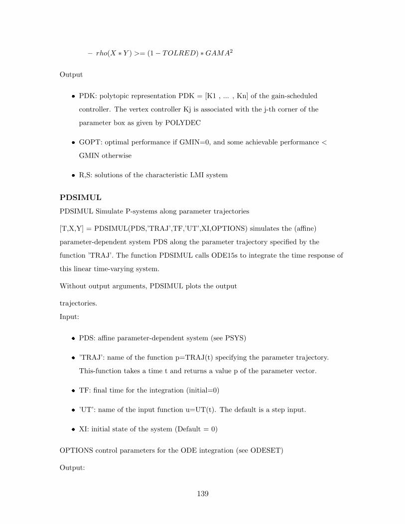
– rho(X ∗ Y ) >= (1− TOLRED) ∗GAMA2
Output
� PDK: polytopic representation PDK = [K1 , ... , Kn] of the gain-scheduled
controller. The vertex controller Kj is associated with the j-th corner of the
parameter box as given by POLYDEC
� GOPT: optimal performance if GMIN=0, and some achievable performance <
GMIN otherwise
� R,S: solutions of the characteristic LMI system
PDSIMUL
PDSIMUL Simulate P-systems along parameter trajectories
[T,X,Y] = PDSIMUL(PDS,’TRAJ’,TF,’UT’,XI,OPTIONS) simulates the (affine)
parameter-dependent system PDS along the parameter trajectory specified by the
function ’TRAJ’. The function PDSIMUL calls ODE15s to integrate the time response of
this linear time-varying system.
Without output arguments, PDSIMUL plots the output
trajectories.
Input:
� PDS: affine parameter-dependent system (see PSYS)
� ’TRAJ’: name of the function p=TRAJ(t) specifying the parameter trajectory.
This-function takes a time t and returns a value p of the parameter vector.
� TF: final time for the integration (initial=0)
� ’UT’: name of the input function u=UT(t). The default is a step input.
� XI: initial state of the system (Default = 0)
OPTIONS control parameters for the ODE integration (see ODESET)
Output:
139
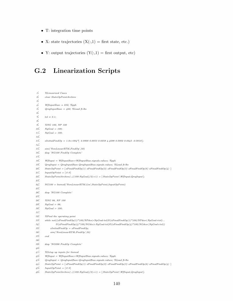
� T: integration time points
� X: state trajectories (X(:,1) = first state, etc.)
� Y: output trajectories (Y(:,1) = first output, etc)
G.2 Linearization Scripts
1: %Linearized Cases
2: clear StateOpPointArchive
3:4: WfInputBase = 832; %pph
5: QreqInputBase = 460; %Load ft-lbs
6:7: tol = 0.1;
8:9: %NG 100, NP 100
10: NgGoal = 100;
11: NpGoal = 100;
12:13: xInitialFindOp = 1.0e+004*[ 2.0900 0.0053 0.0258 4.4698 0.0002 0.0245 -0.0010 ];
14:15: sim(’NonLinearRTM FindOp’,50)
16: disp ’NG100 FindOp Complete’
17:18: WfInput = WfInputBase+WfInputBias.signals.values; %pph
19: QreqInput = QreqInputBase-QreqInputBias.signals.values; %Load ft-lbs
20: StateOpPoint = [ xFinalFindOp(1) xFinalFindOp(2) xFinalFindOp(3) xFinalFindOp(6) xFinalFindOp(4) ]
21: InputOpPoint = [ 0 0 ]
22: StateOpPointArchive(:,((100-NgGoal)/2)+1) = [ StateOpPoint’;WfInput;QreqInput ];
23:24: NG100 = linmod(’NonLinearRTM Lin’,StateOpPoint,InputOpPoint)
25:26: disp ’NG100 Complete’
27:28: %NG 98, NP 100
29: NgGoal = 98;
30: NpGoal = 100;
31:32: %Find the operating point
33: while not((xFinalFindOp(1)*100/NPdes>NpGoal-tol)&(xFinalFindOp(1)*100/NPdes<NpGoal+tol)...
34: &(xFinalFindOp(4)*100/NGdes>NgGoal-tol)&(xFinalFindOp(4)*100/NGdes<NgGoal+tol))
35: xInitialFindOp = xFinalFindOp;
36: sim(’NonLinearRTM FindOp’,50)
37: end
38:39: disp ’NG098 FindOp Complete’
40:41: %Setup up inputs for linmod
42: WfInput = WfInputBase+WfInputBias.signals.values; %pph
43: QreqInput = QreqInputBase-QreqInputBias.signals.values; %Load ft-lbs
44: StateOpPoint = [ xFinalFindOp(1) xFinalFindOp(2) xFinalFindOp(3) xFinalFindOp(6) xFinalFindOp(4) ]
45: InputOpPoint = [ 0 0 ]
46: StateOpPointArchive(:,((100-NgGoal)/2)+1) = [ StateOpPoint’;WfInput;QreqInput ];
140
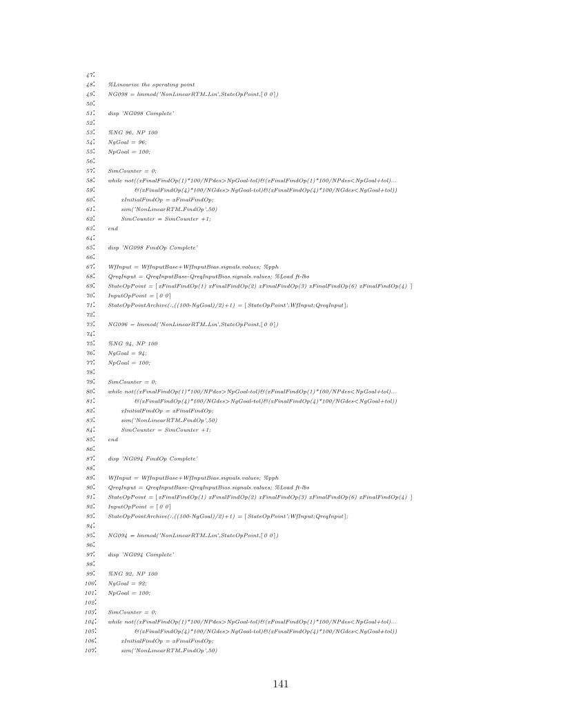
47:48: %Linearize the operating point
49: NG098 = linmod(’NonLinearRTM Lin’,StateOpPoint,[ 0 0 ])
50:51: disp ’NG098 Complete’
52:53: %NG 96, NP 100
54: NgGoal = 96;
55: NpGoal = 100;
56:57: SimCounter = 0;
58: while not((xFinalFindOp(1)*100/NPdes>NpGoal-tol)&(xFinalFindOp(1)*100/NPdes<NpGoal+tol)...
59: &(xFinalFindOp(4)*100/NGdes>NgGoal-tol)&(xFinalFindOp(4)*100/NGdes<NgGoal+tol))
60: xInitialFindOp = xFinalFindOp;
61: sim(’NonLinearRTM FindOp’,50)
62: SimCounter = SimCounter +1;
63: end
64:65: disp ’NG098 FindOp Complete’
66:67: WfInput = WfInputBase+WfInputBias.signals.values; %pph
68: QreqInput = QreqInputBase-QreqInputBias.signals.values; %Load ft-lbs
69: StateOpPoint = [ xFinalFindOp(1) xFinalFindOp(2) xFinalFindOp(3) xFinalFindOp(6) xFinalFindOp(4) ]
70: InputOpPoint = [ 0 0 ]
71: StateOpPointArchive(:,((100-NgGoal)/2)+1) = [ StateOpPoint’;WfInput;QreqInput ];
72:73: NG096 = linmod(’NonLinearRTM Lin’,StateOpPoint,[ 0 0 ])
74:75: %NG 94, NP 100
76: NgGoal = 94;
77: NpGoal = 100;
78:79: SimCounter = 0;
80: while not((xFinalFindOp(1)*100/NPdes>NpGoal-tol)&(xFinalFindOp(1)*100/NPdes<NpGoal+tol)...
81: &(xFinalFindOp(4)*100/NGdes>NgGoal-tol)&(xFinalFindOp(4)*100/NGdes<NgGoal+tol))
82: xInitialFindOp = xFinalFindOp;
83: sim(’NonLinearRTM FindOp’,50)
84: SimCounter = SimCounter +1;
85: end
86:87: disp ’NG094 FindOp Complete’
88:89: WfInput = WfInputBase+WfInputBias.signals.values; %pph
90: QreqInput = QreqInputBase-QreqInputBias.signals.values; %Load ft-lbs
91: StateOpPoint = [ xFinalFindOp(1) xFinalFindOp(2) xFinalFindOp(3) xFinalFindOp(6) xFinalFindOp(4) ]
92: InputOpPoint = [ 0 0 ]
93: StateOpPointArchive(:,((100-NgGoal)/2)+1) = [ StateOpPoint’;WfInput;QreqInput ];
94:95: NG094 = linmod(’NonLinearRTM Lin’,StateOpPoint,[ 0 0 ])
96:97: disp ’NG094 Complete’
98:99: %NG 92, NP 100
100: NgGoal = 92;
101: NpGoal = 100;
102:103: SimCounter = 0;
104: while not((xFinalFindOp(1)*100/NPdes>NpGoal-tol)&(xFinalFindOp(1)*100/NPdes<NpGoal+tol)...
105: &(xFinalFindOp(4)*100/NGdes>NgGoal-tol)&(xFinalFindOp(4)*100/NGdes<NgGoal+tol))
106: xInitialFindOp = xFinalFindOp;
107: sim(’NonLinearRTM FindOp’,50)
141
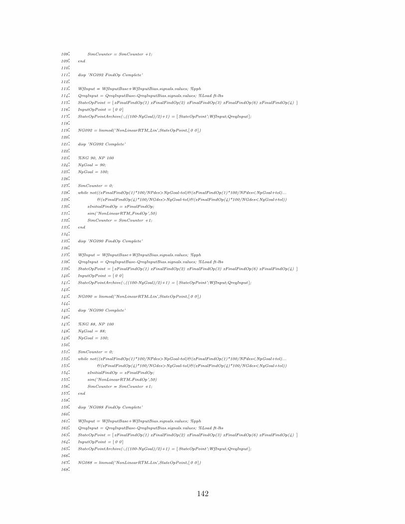
108: SimCounter = SimCounter +1;
109: end
110:111: disp ’NG092 FindOp Complete’
112:113: WfInput = WfInputBase+WfInputBias.signals.values; %pph
114: QreqInput = QreqInputBase-QreqInputBias.signals.values; %Load ft-lbs
115: StateOpPoint = [ xFinalFindOp(1) xFinalFindOp(2) xFinalFindOp(3) xFinalFindOp(6) xFinalFindOp(4) ]
116: InputOpPoint = [ 0 0 ]
117: StateOpPointArchive(:,((100-NgGoal)/2)+1) = [ StateOpPoint’;WfInput;QreqInput ];
118:119: NG092 = linmod(’NonLinearRTM Lin’,StateOpPoint,[ 0 0 ])
120:121: disp ’NG092 Complete’
122:123: %NG 90, NP 100
124: NgGoal = 90;
125: NpGoal = 100;
126:127: SimCounter = 0;
128: while not((xFinalFindOp(1)*100/NPdes>NpGoal-tol)&(xFinalFindOp(1)*100/NPdes<NpGoal+tol)...
129: &(xFinalFindOp(4)*100/NGdes>NgGoal-tol)&(xFinalFindOp(4)*100/NGdes<NgGoal+tol))
130: xInitialFindOp = xFinalFindOp;
131: sim(’NonLinearRTM FindOp’,50)
132: SimCounter = SimCounter +1;
133: end
134:135: disp ’NG090 FindOp Complete’
136:137: WfInput = WfInputBase+WfInputBias.signals.values; %pph
138: QreqInput = QreqInputBase-QreqInputBias.signals.values; %Load ft-lbs
139: StateOpPoint = [ xFinalFindOp(1) xFinalFindOp(2) xFinalFindOp(3) xFinalFindOp(6) xFinalFindOp(4) ]
140: InputOpPoint = [ 0 0 ]
141: StateOpPointArchive(:,((100-NgGoal)/2)+1) = [ StateOpPoint’;WfInput;QreqInput ];
142:143: NG090 = linmod(’NonLinearRTM Lin’,StateOpPoint,[ 0 0 ])
144:145: disp ’NG090 Complete’
146:147: %NG 88, NP 100
148: NgGoal = 88;
149: NpGoal = 100;
150:151: SimCounter = 0;
152: while not((xFinalFindOp(1)*100/NPdes>NpGoal-tol)&(xFinalFindOp(1)*100/NPdes<NpGoal+tol)...
153: &(xFinalFindOp(4)*100/NGdes>NgGoal-tol)&(xFinalFindOp(4)*100/NGdes<NgGoal+tol))
154: xInitialFindOp = xFinalFindOp;
155: sim(’NonLinearRTM FindOp’,50)
156: SimCounter = SimCounter +1;
157: end
158:159: disp ’NG088 FindOp Complete’
160:161: WfInput = WfInputBase+WfInputBias.signals.values; %pph
162: QreqInput = QreqInputBase-QreqInputBias.signals.values; %Load ft-lbs
163: StateOpPoint = [ xFinalFindOp(1) xFinalFindOp(2) xFinalFindOp(3) xFinalFindOp(6) xFinalFindOp(4) ]
164: InputOpPoint = [ 0 0 ]
165: StateOpPointArchive(:,((100-NgGoal)/2)+1) = [ StateOpPoint’;WfInput;QreqInput ];
166:167: NG088 = linmod(’NonLinearRTM Lin’,StateOpPoint,[ 0 0 ])
168:
142
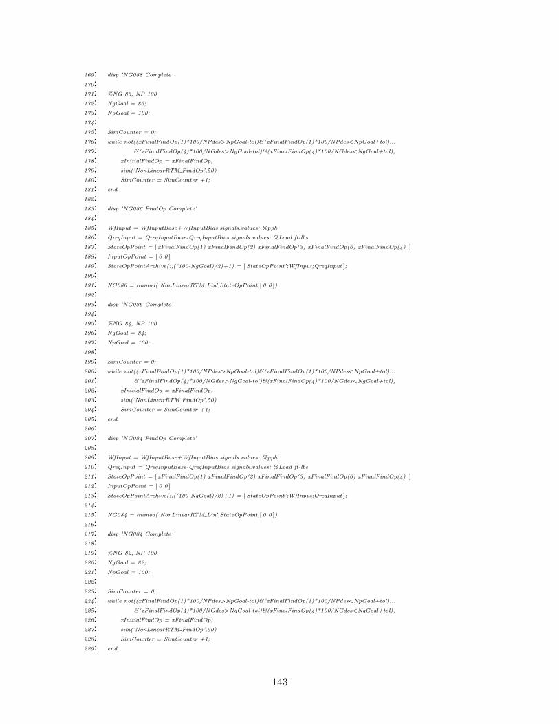
169: disp ’NG088 Complete’
170:171: %NG 86, NP 100
172: NgGoal = 86;
173: NpGoal = 100;
174:175: SimCounter = 0;
176: while not((xFinalFindOp(1)*100/NPdes>NpGoal-tol)&(xFinalFindOp(1)*100/NPdes<NpGoal+tol)...
177: &(xFinalFindOp(4)*100/NGdes>NgGoal-tol)&(xFinalFindOp(4)*100/NGdes<NgGoal+tol))
178: xInitialFindOp = xFinalFindOp;
179: sim(’NonLinearRTM FindOp’,50)
180: SimCounter = SimCounter +1;
181: end
182:183: disp ’NG086 FindOp Complete’
184:185: WfInput = WfInputBase+WfInputBias.signals.values; %pph
186: QreqInput = QreqInputBase-QreqInputBias.signals.values; %Load ft-lbs
187: StateOpPoint = [ xFinalFindOp(1) xFinalFindOp(2) xFinalFindOp(3) xFinalFindOp(6) xFinalFindOp(4) ]
188: InputOpPoint = [ 0 0 ]
189: StateOpPointArchive(:,((100-NgGoal)/2)+1) = [ StateOpPoint’;WfInput;QreqInput ];
190:191: NG086 = linmod(’NonLinearRTM Lin’,StateOpPoint,[ 0 0 ])
192:193: disp ’NG086 Complete’
194:195: %NG 84, NP 100
196: NgGoal = 84;
197: NpGoal = 100;
198:199: SimCounter = 0;
200: while not((xFinalFindOp(1)*100/NPdes>NpGoal-tol)&(xFinalFindOp(1)*100/NPdes<NpGoal+tol)...
201: &(xFinalFindOp(4)*100/NGdes>NgGoal-tol)&(xFinalFindOp(4)*100/NGdes<NgGoal+tol))
202: xInitialFindOp = xFinalFindOp;
203: sim(’NonLinearRTM FindOp’,50)
204: SimCounter = SimCounter +1;
205: end
206:207: disp ’NG084 FindOp Complete’
208:209: WfInput = WfInputBase+WfInputBias.signals.values; %pph
210: QreqInput = QreqInputBase-QreqInputBias.signals.values; %Load ft-lbs
211: StateOpPoint = [ xFinalFindOp(1) xFinalFindOp(2) xFinalFindOp(3) xFinalFindOp(6) xFinalFindOp(4) ]
212: InputOpPoint = [ 0 0 ]
213: StateOpPointArchive(:,((100-NgGoal)/2)+1) = [ StateOpPoint’;WfInput;QreqInput ];
214:215: NG084 = linmod(’NonLinearRTM Lin’,StateOpPoint,[ 0 0 ])
216:217: disp ’NG084 Complete’
218:219: %NG 82, NP 100
220: NgGoal = 82;
221: NpGoal = 100;
222:223: SimCounter = 0;
224: while not((xFinalFindOp(1)*100/NPdes>NpGoal-tol)&(xFinalFindOp(1)*100/NPdes<NpGoal+tol)...
225: &(xFinalFindOp(4)*100/NGdes>NgGoal-tol)&(xFinalFindOp(4)*100/NGdes<NgGoal+tol))
226: xInitialFindOp = xFinalFindOp;
227: sim(’NonLinearRTM FindOp’,50)
228: SimCounter = SimCounter +1;
229: end
143
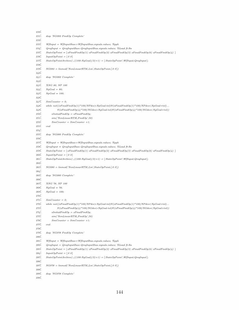
230:231: disp ’NG082 FindOp Complete’
232:233: WfInput = WfInputBase+WfInputBias.signals.values; %pph
234: QreqInput = QreqInputBase-QreqInputBias.signals.values; %Load ft-lbs
235: StateOpPoint = [ xFinalFindOp(1) xFinalFindOp(2) xFinalFindOp(3) xFinalFindOp(6) xFinalFindOp(4) ]
236: InputOpPoint = [ 0 0 ]
237: StateOpPointArchive(:,((100-NgGoal)/2)+1) = [ StateOpPoint’;WfInput;QreqInput ];
238:239: NG082 = linmod(’NonLinearRTM Lin’,StateOpPoint,[ 0 0 ])
240:241: disp ’NG082 Complete’
242:243: %NG 80, NP 100
244: NgGoal = 80;
245: NpGoal = 100;
246:247: SimCounter = 0;
248: while not((xFinalFindOp(1)*100/NPdes>NpGoal-tol)&(xFinalFindOp(1)*100/NPdes<NpGoal+tol)...
249: &(xFinalFindOp(4)*100/NGdes>NgGoal-tol)&(xFinalFindOp(4)*100/NGdes<NgGoal+tol))
250: xInitialFindOp = xFinalFindOp;
251: sim(’NonLinearRTM FindOp’,50)
252: SimCounter = SimCounter +1;
253: end
254:255: disp ’NG080 FindOp Complete’
256:257: WfInput = WfInputBase+WfInputBias.signals.values; %pph
258: QreqInput = QreqInputBase-QreqInputBias.signals.values; %Load ft-lbs
259: StateOpPoint = [ xFinalFindOp(1) xFinalFindOp(2) xFinalFindOp(3) xFinalFindOp(6) xFinalFindOp(4) ]
260: InputOpPoint = [ 0 0 ]
261: StateOpPointArchive(:,((100-NgGoal)/2)+1) = [ StateOpPoint’;WfInput;QreqInput ];
262:263: NG080 = linmod(’NonLinearRTM Lin’,StateOpPoint,[ 0 0 ])
264:265: disp ’NG080 Complete’
266:267: %NG 78, NP 100
268: NgGoal = 78;
269: NpGoal = 100;
270:271: SimCounter = 0;
272: while not((xFinalFindOp(1)*100/NPdes>NpGoal-tol)&(xFinalFindOp(1)*100/NPdes<NpGoal+tol)...
273: &(xFinalFindOp(4)*100/NGdes>NgGoal-tol)&(xFinalFindOp(4)*100/NGdes<NgGoal+tol))
274: xInitialFindOp = xFinalFindOp;
275: sim(’NonLinearRTM FindOp’,50)
276: SimCounter = SimCounter +1;
277: end
278:279: disp ’NG078 FindOp Complete’
280:281: WfInput = WfInputBase+WfInputBias.signals.values; %pph
282: QreqInput = QreqInputBase-QreqInputBias.signals.values; %Load ft-lbs
283: StateOpPoint = [ xFinalFindOp(1) xFinalFindOp(2) xFinalFindOp(3) xFinalFindOp(6) xFinalFindOp(4) ]
284: InputOpPoint = [ 0 0 ]
285: StateOpPointArchive(:,((100-NgGoal)/2)+1) = [ StateOpPoint’;WfInput;QreqInput ];
286:287: NG078 = linmod(’NonLinearRTM Lin’,StateOpPoint,[ 0 0 ])
288:289: disp ’NG078 Complete’
290:
144
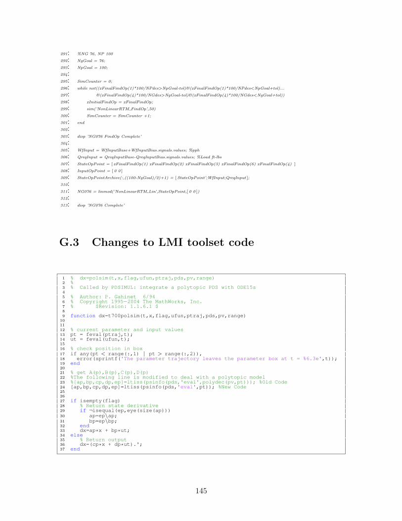
291: %NG 76, NP 100
292: NgGoal = 76;
293: NpGoal = 100;
294:295: SimCounter = 0;
296: while not((xFinalFindOp(1)*100/NPdes>NpGoal-tol)&(xFinalFindOp(1)*100/NPdes<NpGoal+tol)...
297: &(xFinalFindOp(4)*100/NGdes>NgGoal-tol)&(xFinalFindOp(4)*100/NGdes<NgGoal+tol))
298: xInitialFindOp = xFinalFindOp;
299: sim(’NonLinearRTM FindOp’,50)
300: SimCounter = SimCounter +1;
301: end
302:303: disp ’NG076 FindOp Complete’
304:305: WfInput = WfInputBase+WfInputBias.signals.values; %pph
306: QreqInput = QreqInputBase-QreqInputBias.signals.values; %Load ft-lbs
307: StateOpPoint = [ xFinalFindOp(1) xFinalFindOp(2) xFinalFindOp(3) xFinalFindOp(6) xFinalFindOp(4) ]
308: InputOpPoint = [ 0 0 ]
309: StateOpPointArchive(:,((100-NgGoal)/2)+1) = [ StateOpPoint’;WfInput;QreqInput ];
310:311: NG076 = linmod(’NonLinearRTM Lin’,StateOpPoint,[ 0 0 ])
312:313: disp ’NG076 Complete’
G.3 Changes to LMI toolset code
1 % dx=polsim(t,x,flag,ufun,ptraj,pds,pv,range)2 %3 % Called by PDSIMUL: integrate a polytopic PDS with ODE15s45 % Author: P. Gahinet 6/946 % Copyright 1995−2004 The MathWorks, Inc.7 % $Revision: 1.1.6.1 $89 function dx=t700polsim(t,x,flag,ufun,ptraj,pds,pv,range)
101112 % current parameter and input values13 pt = feval(ptraj,t);14 ut = feval(ufun,t);1516 % check position in box17 if any(pt < range(:,1) | pt > range(:,2)),18 error(sprintf('The parameter trajectory leaves the parameter box at t = %6.3e',t));19 end2021 % get A(p),B(p),C(p),D(p)22 %The following line is modified to deal with a polytopic model23 %[ap,bp,cp,dp,ep]=ltiss(psinfo(pds,'eval',polydec(pv,pt))); %Old Code24 [ap,bp,cp,dp,ep]=ltiss(psinfo(pds,'eval',pt)); %New Code252627 if isempty(flag)28 % Return state derivative29 if ¬isequal(ep,eye(size(ap)))30 ap=ep\ap;31 bp=ep\bp;32 end33 dx=ap*x + bp*ut;34 else35 % Return output36 dx=(cp*x + dp*ut).';37 end
145
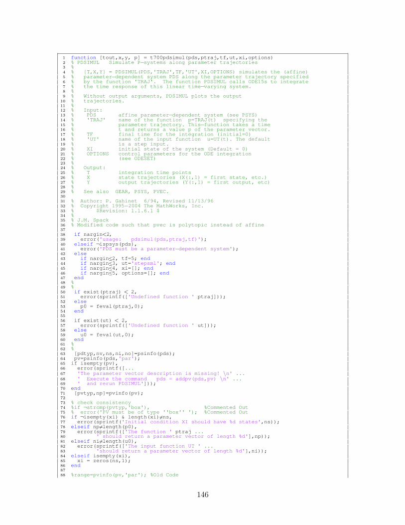
1 function [tout,x,y, p] = t700pdsimul(pds,ptraj,tf,ut,xi,options)2 % PDSIMUL Simulate P−systems along parameter trajectories3 %4 % [T,X,Y] = PDSIMUL(PDS,'TRAJ',TF,'UT',XI,OPTIONS) simulates the (affine)5 % parameter−dependent system PDS along the parameter trajectory specified6 % by the function 'TRAJ'. The function PDSIMUL calls ODE15s to integrate7 % the time response of this linear time−varying system.8 %9 % Without output arguments, PDSIMUL plots the output
10 % trajectories.11 %12 % Input:13 % PDS affine parameter−dependent system (see PSYS)14 % 'TRAJ' name of the function p=TRAJ(t) specifying the15 % parameter trajectory. This−function takes a time16 % t and returns a value p of the parameter vector.17 % TF final time for the integration (initial=0)18 % 'UT' name of the input function u=UT(t). The default19 % is a step input.20 % XI initial state of the system (Default = 0)21 % OPTIONS control parameters for the ODE integration22 % (see ODESET)23 %24 % Output:25 % T integration time points26 % X state trajectories (X(:,1) = first state, etc.)27 % Y output trajectories (Y(:,1) = first output, etc)28 %29 % See also GEAR, PSYS, PVEC.3031 % Author: P. Gahinet 6/94, Revised 11/13/9632 % Copyright 1995−2004 The MathWorks, Inc.33 % $Revision: 1.1.6.1 $34 %35 % J.M. Spack36 % Modified code such that pvec is polytopic instead of affine3738 if nargin<2,39 error('usage: pdsimul(pds,ptraj,tf)');40 elseif ¬ispsys(pds),41 error('PDS must be a parameter−dependent system');42 else43 if nargin≤2, tf=5; end44 if nargin≤3, ut='stepsml'; end45 if nargin≤4, xi=[]; end46 if nargin≤5, options=[]; end47 end48 %49 %50 if exist(ptraj) < 2,51 error(sprintf(['Undefined function ' ptraj]));52 else53 p0 = feval(ptraj,0);54 end5556 if exist(ut) < 2,57 error(sprintf(['Undefined function ' ut]));58 else59 u0 = feval(ut,0);60 end61 %62 %63 [pdtyp,nv,ns,ni,no]=psinfo(pds);64 pv=psinfo(pds,'par');65 if isempty(pv),66 error(sprintf([...67 'The parameter vector description is missing! \n' ...68 ' Execute the command pds = addpv(pds,pv) \n' ...69 ' and rerun PDSIMUL']));70 end71 [pvtyp,np]=pvinfo(pv);7273 % check consistency74 %if ¬strcmp(pvtyp,'box'), %Commented Out75 % error('PV must be of type ''box'' '); %Commented Out76 if ¬isempty(xi) & length(xi)6=ns,77 error(sprintf('Initial condition XI should have %d states',ns));78 elseif np6=length(p0),79 error(sprintf(['The function ' ptraj ...80 ' should return a parameter vector of length %d'],np));81 elseif ni6=length(u0),82 error(sprintf(['The input function UT ' ...83 'should return a parameter vector of length %d'],ni));84 elseif isempty(xi),85 xi = zeros(ns,1);86 end8788 %range=pvinfo(pv,'par'); %Old Code
146
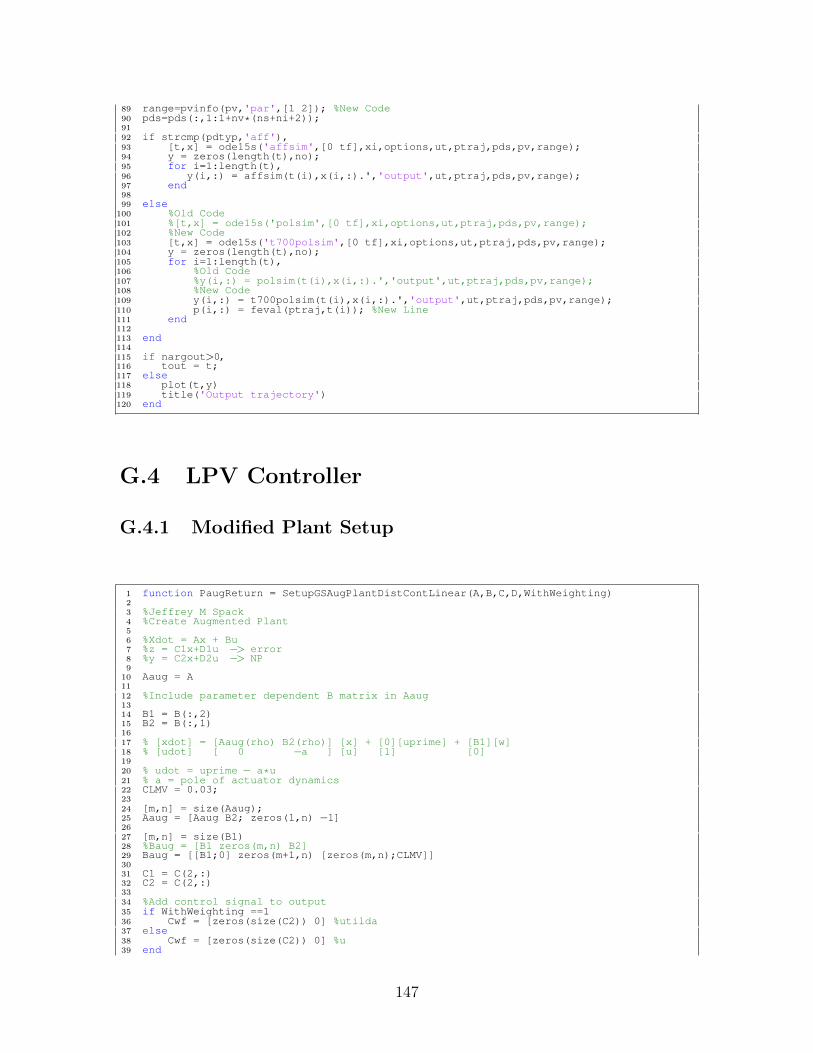
89 range=pvinfo(pv,'par',[1 2]); %New Code90 pds=pds(:,1:1+nv*(ns+ni+2));9192 if strcmp(pdtyp,'aff'),93 [t,x] = ode15s('affsim',[0 tf],xi,options,ut,ptraj,pds,pv,range);94 y = zeros(length(t),no);95 for i=1:length(t),96 y(i,:) = affsim(t(i),x(i,:).','output',ut,ptraj,pds,pv,range);97 end9899 else
100 %Old Code101 %[t,x] = ode15s('polsim',[0 tf],xi,options,ut,ptraj,pds,pv,range);102 %New Code103 [t,x] = ode15s('t700polsim',[0 tf],xi,options,ut,ptraj,pds,pv,range);104 y = zeros(length(t),no);105 for i=1:length(t),106 %Old Code107 %y(i,:) = polsim(t(i),x(i,:).','output',ut,ptraj,pds,pv,range);108 %New Code109 y(i,:) = t700polsim(t(i),x(i,:).','output',ut,ptraj,pds,pv,range);110 p(i,:) = feval(ptraj,t(i)); %New Line111 end112113 end114115 if nargout>0,116 tout = t;117 else118 plot(t,y)119 title('Output trajectory')120 end
G.4 LPV Controller
G.4.1 Modified Plant Setup
1 function PaugReturn = SetupGSAugPlantDistContLinear(A,B,C,D,WithWeighting)23 %Jeffrey M Spack4 %Create Augmented Plant56 %Xdot = Ax + Bu7 %z = C1x+D1u −> error8 %y = C2x+D2u −> NP9
10 Aaug = A1112 %Include parameter dependent B matrix in Aaug1314 B1 = B(:,2)15 B2 = B(:,1)1617 % [xdot] = [Aaug(rho) B2(rho)] [x] + [0][uprime] + [B1][w]18 % [udot] [ 0 −a ] [u] [1] [0]1920 % udot = uprime − a*u21 % a = pole of actuator dynamics22 CLMV = 0.03;2324 [m,n] = size(Aaug);25 Aaug = [Aaug B2; zeros(1,n) −1]2627 [m,n] = size(B1)28 %Baug = [B1 zeros(m,n) B2]29 Baug = [[B1;0] zeros(m+1,n) [zeros(m,n);CLMV]]3031 C1 = C(2,:)32 C2 = C(2,:)3334 %Add control signal to output35 if WithWeighting ==136 Cwf = [zeros(size(C2)) 0] %utilda37 else38 Cwf = [zeros(size(C2)) 0] %u39 end
147
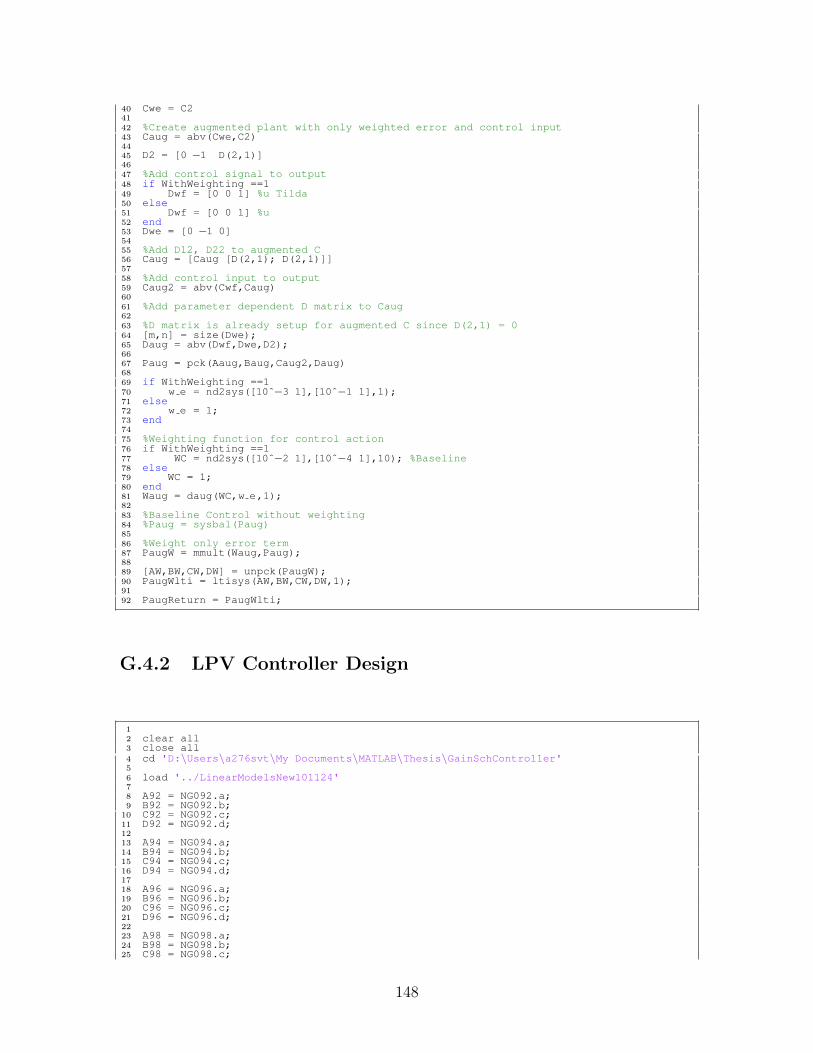
40 Cwe = C24142 %Create augmented plant with only weighted error and control input43 Caug = abv(Cwe,C2)4445 D2 = [0 −1 D(2,1)]4647 %Add control signal to output48 if WithWeighting ==149 Dwf = [0 0 1] %u Tilda50 else51 Dwf = [0 0 1] %u52 end53 Dwe = [0 −1 0]5455 %Add D12, D22 to augmented C56 Caug = [Caug [D(2,1); D(2,1)]]5758 %Add control input to output59 Caug2 = abv(Cwf,Caug)6061 %Add parameter dependent D matrix to Caug6263 %D matrix is already setup for augmented C since D(2,1) = 064 [m,n] = size(Dwe);65 Daug = abv(Dwf,Dwe,D2);6667 Paug = pck(Aaug,Baug,Caug2,Daug)6869 if WithWeighting ==170 w e = nd2sys([10ˆ−3 1],[10ˆ−1 1],1);71 else72 w e = 1;73 end7475 %Weighting function for control action76 if WithWeighting ==177 WC = nd2sys([10ˆ−2 1],[10ˆ−4 1],10); %Baseline78 else79 WC = 1;80 end81 Waug = daug(WC,w e,1);8283 %Baseline Control without weighting84 %Paug = sysbal(Paug)8586 %Weight only error term87 PaugW = mmult(Waug,Paug);8889 [AW,BW,CW,DW] = unpck(PaugW);90 PaugWlti = ltisys(AW,BW,CW,DW,1);9192 PaugReturn = PaugWlti;
G.4.2 LPV Controller Design
12 clear all3 close all4 cd 'D:\Users\a276svt\My Documents\MATLAB\Thesis\GainSchController'56 load '../LinearModelsNew101124'78 A92 = NG092.a;9 B92 = NG092.b;
10 C92 = NG092.c;11 D92 = NG092.d;1213 A94 = NG094.a;14 B94 = NG094.b;15 C94 = NG094.c;16 D94 = NG094.d;1718 A96 = NG096.a;19 B96 = NG096.b;20 C96 = NG096.c;21 D96 = NG096.d;2223 A98 = NG098.a;24 B98 = NG098.b;25 C98 = NG098.c;
148
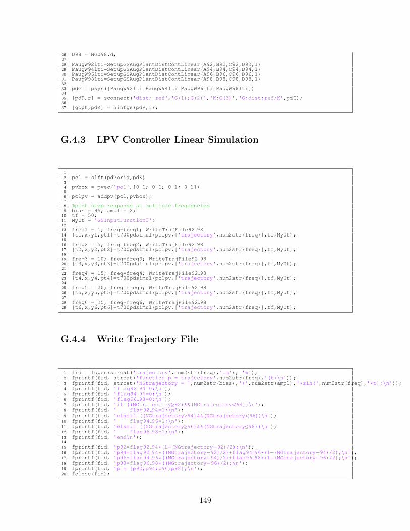
26 D98 = NG098.d;2728 PaugW92lti=SetupGSAugPlantDistContLinear(A92,B92,C92,D92,1)29 PaugW94lti=SetupGSAugPlantDistContLinear(A94,B94,C94,D94,1)30 PaugW96lti=SetupGSAugPlantDistContLinear(A96,B96,C96,D96,1)31 PaugW98lti=SetupGSAugPlantDistContLinear(A98,B98,C98,D98,1)3233 pdG = psys([PaugW92lti PaugW94lti PaugW96lti PaugW98lti])3435 [pdP,r] = sconnect('dist; ref','G(1);G(2)','K:G(3)','G:dist;ref;K',pdG);3637 [gopt,pdK] = hinfgs(pdP,r);
G.4.3 LPV Controller Linear Simulation
12 pcl = slft(pdPorig,pdK)34 pvbox = pvec('pol',[0 1; 0 1; 0 1; 0 1])56 pclpv = addpv(pcl,pvbox);78 %plot step response at multiple frequencies9 bias = 95; ampl = 2;
10 tf = 50;11 MyUt = 'GSInputFunction2';1213 freq1 = 1; freq=freq1; WriteTrajFile92 9814 [t1,x,y1,pt1]=t700pdsimul(pclpv,['trajectory',num2str(freq)],tf,MyUt);1516 freq2 = 5; freq=freq2; WriteTrajFile92 9817 [t2,x,y2,pt2]=t700pdsimul(pclpv,['trajectory',num2str(freq)],tf,MyUt);1819 freq3 = 10; freq=freq3; WriteTrajFile92 9820 [t3,x,y3,pt3]=t700pdsimul(pclpv,['trajectory',num2str(freq)],tf,MyUt);2122 freq4 = 15; freq=freq4; WriteTrajFile92 9823 [t4,x,y4,pt4]=t700pdsimul(pclpv,['trajectory',num2str(freq)],tf,MyUt);2425 freq5 = 20; freq=freq5; WriteTrajFile92 9826 [t5,x,y5,pt5]=t700pdsimul(pclpv,['trajectory',num2str(freq)],tf,MyUt);2728 freq6 = 25; freq=freq6; WriteTrajFile92 9829 [t6,x,y6,pt6]=t700pdsimul(pclpv,['trajectory',num2str(freq)],tf,MyUt);
G.4.4 Write Trajectory File
1 fid = fopen(strcat('trajectory',num2str(freq),'.m'), 'w');2 fprintf(fid, strcat('function p = trajectory',num2str(freq),'(t)\n'));3 fprintf(fid, strcat('NGtrajectory = ',num2str(bias),'+',num2str(ampl),'*sin(',num2str(freq),'*t);\n'));4 fprintf(fid, 'flag92 94=0;\n');5 fprintf(fid, 'flag94 96=0;\n');6 fprintf(fid, 'flag96 98=0;\n');7 fprintf(fid, 'if ((NGtrajectory≥92)&&(NGtrajectory<94))\n');8 fprintf(fid, ' flag92 94=1;\n');9 fprintf(fid, 'elseif ((NGtrajectory≥94)&&(NGtrajectory<96))\n');
10 fprintf(fid, ' flag94 96=1;\n');11 fprintf(fid, 'elseif ((NGtrajectory≥96)&&(NGtrajectory≤98))\n');12 fprintf(fid, ' flag96 98=1;\n');13 fprintf(fid, 'end\n');14
15 fprintf(fid, 'p92=flag92 94*(1−(NGtrajectory−92)/2);\n');16 fprintf(fid, 'p94=flag92 94*((NGtrajectory−92)/2)+flag94 96*(1−(NGtrajectory−94)/2);\n');17 fprintf(fid, 'p96=flag94 96*((NGtrajectory−94)/2)+flag96 98*(1−(NGtrajectory−96)/2);\n');18 fprintf(fid, 'p98=flag96 98*((NGtrajectory−96)/2);\n');19 fprintf(fid, 'p = [p92;p94;p96;p98];\n');20 fclose(fid);
149
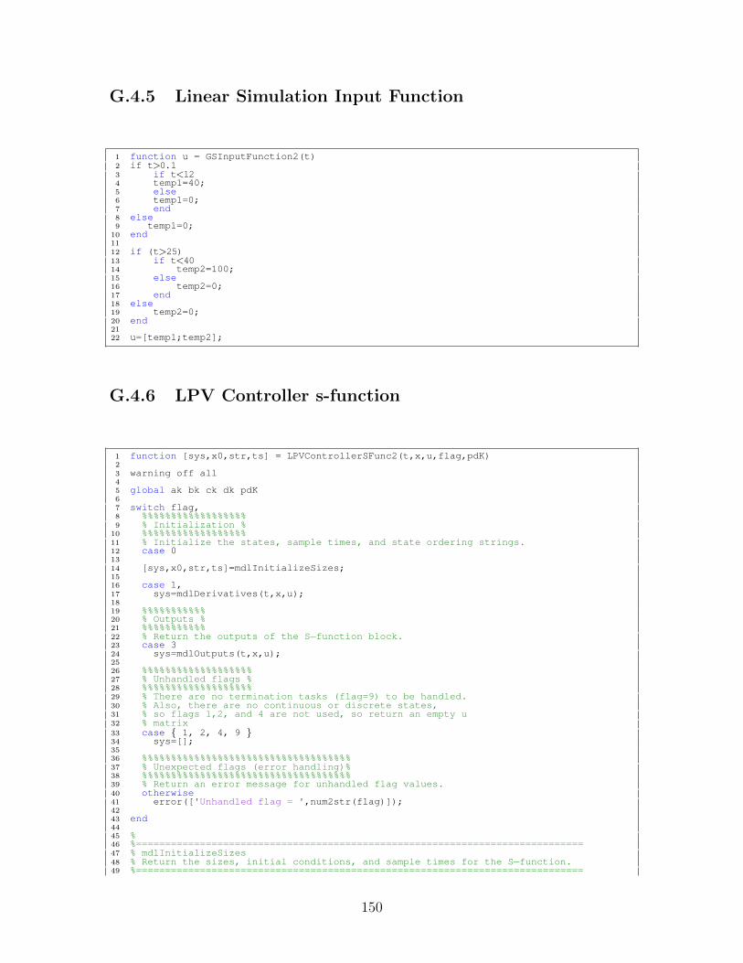
G.4.5 Linear Simulation Input Function
1 function u = GSInputFunction2(t)2 if t>0.13 if t<124 temp1=40;5 else6 temp1=0;7 end8 else9 temp1=0;
10 end1112 if (t>25)13 if t<4014 temp2=100;15 else16 temp2=0;17 end18 else19 temp2=0;20 end2122 u=[temp1;temp2];
G.4.6 LPV Controller s-function
1 function [sys,x0,str,ts] = LPVControllerSFunc2(t,x,u,flag,pdK)23 warning off all45 global ak bk ck dk pdK67 switch flag,8 %%%%%%%%%%%%%%%%%%9 % Initialization %
10 %%%%%%%%%%%%%%%%%%11 % Initialize the states, sample times, and state ordering strings.12 case 01314 [sys,x0,str,ts]=mdlInitializeSizes;1516 case 1,17 sys=mdlDerivatives(t,x,u);1819 %%%%%%%%%%%20 % Outputs %21 %%%%%%%%%%%22 % Return the outputs of the S−function block.23 case 324 sys=mdlOutputs(t,x,u);2526 %%%%%%%%%%%%%%%%%%%27 % Unhandled flags %28 %%%%%%%%%%%%%%%%%%%29 % There are no termination tasks (flag=9) to be handled.30 % Also, there are no continuous or discrete states,31 % so flags 1,2, and 4 are not used, so return an empty u32 % matrix33 case { 1, 2, 4, 9 }34 sys=[];3536 %%%%%%%%%%%%%%%%%%%%%%%%%%%%%%%%%%%%37 % Unexpected flags (error handling)%38 %%%%%%%%%%%%%%%%%%%%%%%%%%%%%%%%%%%%39 % Return an error message for unhandled flag values.40 otherwise41 error(['Unhandled flag = ',num2str(flag)]);4243 end4445 %46 %=============================================================================47 % mdlInitializeSizes48 % Return the sizes, initial conditions, and sample times for the S−function.49 %=============================================================================
150
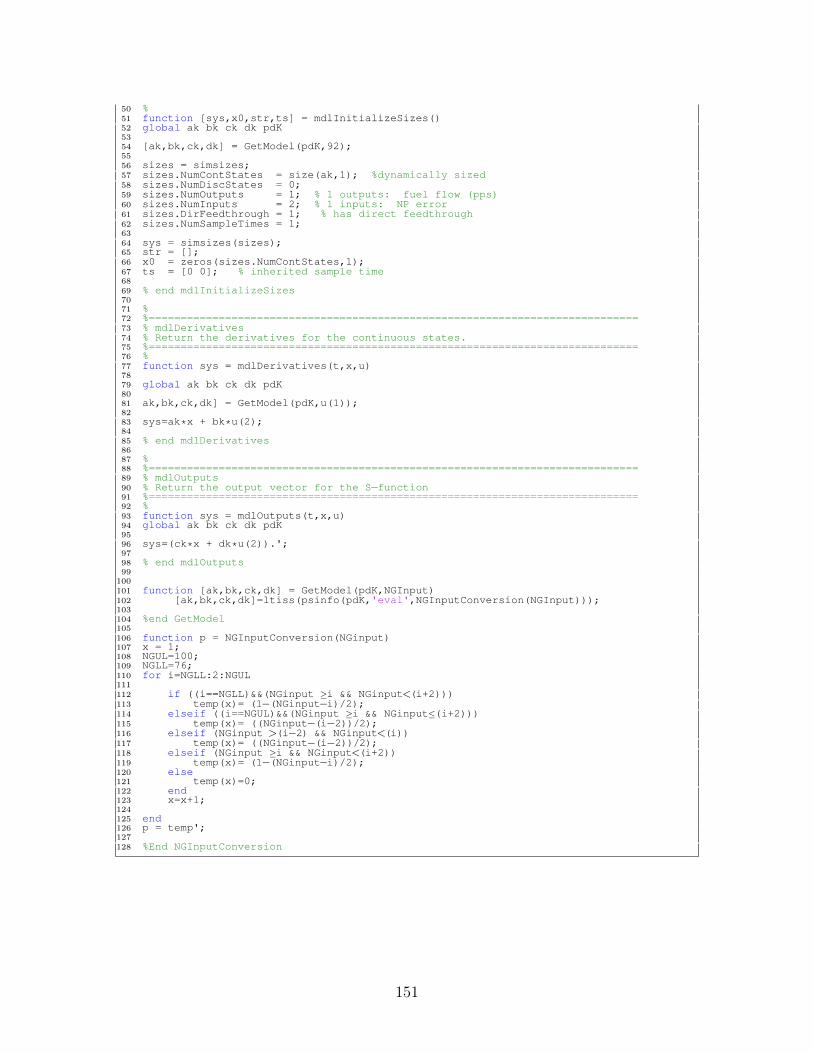
50 %51 function [sys,x0,str,ts] = mdlInitializeSizes()52 global ak bk ck dk pdK5354 [ak,bk,ck,dk] = GetModel(pdK,92);5556 sizes = simsizes;57 sizes.NumContStates = size(ak,1); %dynamically sized58 sizes.NumDiscStates = 0;59 sizes.NumOutputs = 1; % 1 outputs: fuel flow (pps)60 sizes.NumInputs = 2; % 1 inputs: NP error61 sizes.DirFeedthrough = 1; % has direct feedthrough62 sizes.NumSampleTimes = 1;6364 sys = simsizes(sizes);65 str = [];66 x0 = zeros(sizes.NumContStates,1);67 ts = [0 0]; % inherited sample time6869 % end mdlInitializeSizes7071 %72 %=============================================================================73 % mdlDerivatives74 % Return the derivatives for the continuous states.75 %=============================================================================76 %77 function sys = mdlDerivatives(t,x,u)7879 global ak bk ck dk pdK8081 ak,bk,ck,dk] = GetModel(pdK,u(1));8283 sys=ak*x + bk*u(2);8485 % end mdlDerivatives8687 %88 %=============================================================================89 % mdlOutputs90 % Return the output vector for the S−function91 %=============================================================================92 %93 function sys = mdlOutputs(t,x,u)94 global ak bk ck dk pdK9596 sys=(ck*x + dk*u(2)).';9798 % end mdlOutputs99
100101 function [ak,bk,ck,dk] = GetModel(pdK,NGInput)102 [ak,bk,ck,dk]=ltiss(psinfo(pdK,'eval',NGInputConversion(NGInput)));103104 %end GetModel105106 function p = NGInputConversion(NGinput)107 x = 1;108 NGUL=100;109 NGLL=76;110 for i=NGLL:2:NGUL111112 if ((i==NGLL)&&(NGinput ≥i && NGinput<(i+2)))113 temp(x)= (1−(NGinput−i)/2);114 elseif ((i==NGUL)&&(NGinput ≥i && NGinput≤(i+2)))115 temp(x)= ((NGinput−(i−2))/2);116 elseif (NGinput >(i−2) && NGinput<(i))117 temp(x)= ((NGinput−(i−2))/2);118 elseif (NGinput ≥i && NGinput<(i+2))119 temp(x)= (1−(NGinput−i)/2);120 else121 temp(x)=0;122 end123 x=x+1;124125 end126 p = temp';127128 %End NGInputConversion
151
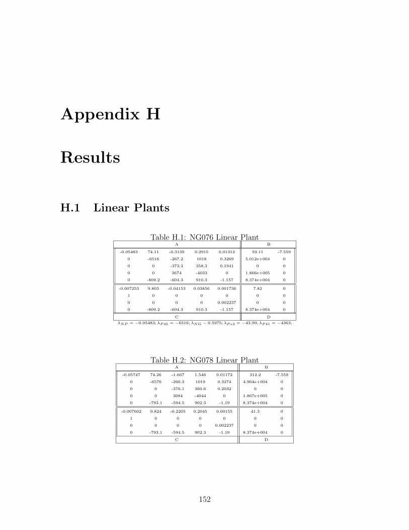
Appendix H
Results
H.1 Linear Plants
Table H.1: NG076 Linear PlantA B
-0.05483 74.11 -0.3139 0.2915 0.01312 59.11 -7.559
0 -6516 -267.2 1018 0.3269 5.012e+004 0
0 0 -373.3 358.3 0.1941 0 0
0 0 3674 -4033 0 1.866e+005 0
0 -809.2 -604.3 910.3 -1.157 8.374e+004 0
-0.007253 9.803 -0.04153 0.03856 0.001736 7.82 0
1 0 0 0 0 0 0
0 0 0 0 0.002237 0 0
0 -809.2 -604.3 910.3 -1.157 8.374e+004 0
C D
λNP = −0.05483;λP45 = −6516;λNG − 0.5975;λPs3 = −43.99;λP41 = −4363;
Table H.2: NG078 Linear PlantA B
-0.05747 74.26 -1.667 1.546 0.01172 312.2 -7.559
0 -6576 -266.3 1019 0.3274 4.964e+004 0
0 0 -376.1 360.6 0.2032 0 0
0 0 3684 -4044 0 1.867e+005 0
0 -793.1 -594.5 902.3 -1.19 8.374e+004 0
-0.007602 9.824 -0.2205 0.2045 0.00155 41.3 0
1 0 0 0 0 0 0
0 0 0 0 0.002237 0 0
0 -793.1 -594.5 902.3 -1.19 8.374e+004 0
C D
152
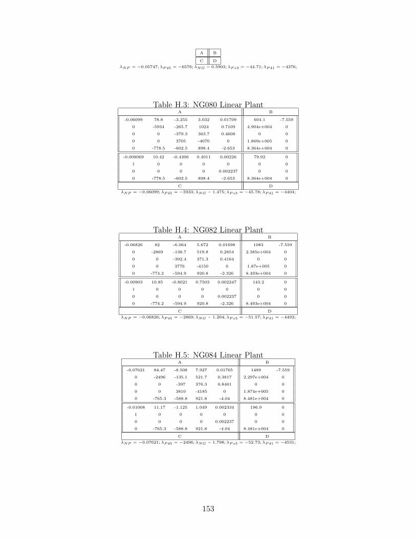
A B
C D
λNP = −0.05747;λP45 = −6576;λNG − 0.5903;λPs3 = −44.71;λP41 = −4376;
Table H.3: NG080 Linear PlantA B
-0.06099 78.8 -3.255 3.032 0.01709 604.1 -7.559
0 -5934 -265.7 1024 0.7109 4.904e+004 0
0 0 -379.3 363.7 0.4608 0 0
0 0 3705 -4070 0 1.869e+005 0
0 -778.5 -602.5 898.4 -2.653 8.364e+004 0
-0.008069 10.42 -0.4306 0.4011 0.00226 79.92 0
1 0 0 0 0 0 0
0 0 0 0 0.002237 0 0
0 -778.5 -602.5 898.4 -2.653 8.364e+004 0
C D
λNP = −0.06099;λP45 = −5933;λNG − 1.475;λPs3 = −45.78;λP41 = −4404;
Table H.4: NG082 Linear PlantA B
-0.06826 82 -6.064 5.672 0.01698 1083 -7.559
0 -2869 -138.7 519.8 0.2854 2.385e+004 0
0 0 -392.4 371.3 0.4164 0 0
0 0 3776 -4150 0 1.87e+005 0
0 -774.2 -594.9 920.8 -2.326 8.493e+004 0
-0.00903 10.85 -0.8021 0.7503 0.002247 143.2 0
1 0 0 0 0 0 0
0 0 0 0 0.002237 0 0
0 -774.2 -594.9 920.8 -2.326 8.493e+004 0
C D
λNP = −0.06826;λP45 = −2869;λNG − 1.204;λPs3 = −51.57;λP41 = −4492;
Table H.5: NG084 Linear PlantA B
-0.07621 84.47 -8.508 7.927 0.01765 1489 -7.559
0 -2496 -135.1 521.7 0.3817 2.297e+004 0
0 0 -397 376.3 0.8461 0 0
0 0 3810 -4185 0 1.874e+005 0
0 -765.3 -588.8 921.8 -4.04 8.481e+004 0
-0.01008 11.17 -1.125 1.049 0.002334 196.9 0
1 0 0 0 0 0 0
0 0 0 0 0.002237 0 0
0 -765.3 -588.8 921.8 -4.04 8.481e+004 0
C D
λNP = −0.07621;λP45 = −2496;λNG − 1.798;λPs3 = −52.73;λP41 = −4531;
153
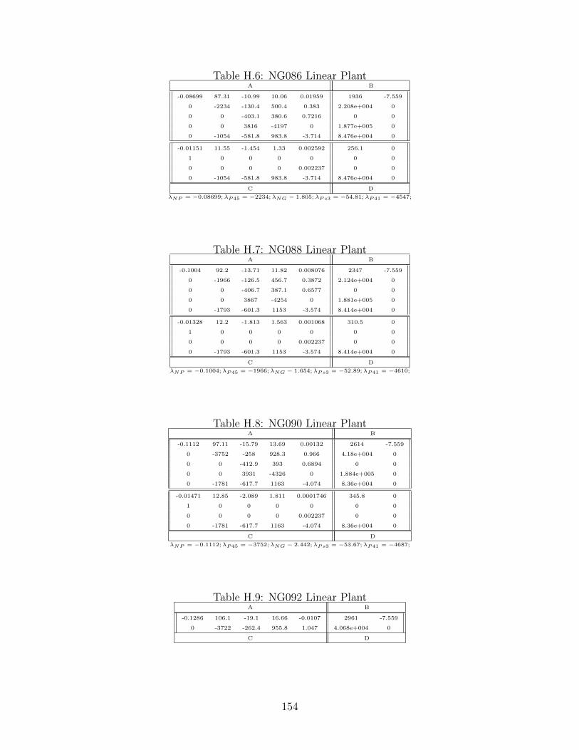
Table H.6: NG086 Linear PlantA B
-0.08699 87.31 -10.99 10.06 0.01959 1936 -7.559
0 -2234 -130.4 500.4 0.383 2.208e+004 0
0 0 -403.1 380.6 0.7216 0 0
0 0 3816 -4197 0 1.877e+005 0
0 -1054 -581.8 983.8 -3.714 8.476e+004 0
-0.01151 11.55 -1.454 1.33 0.002592 256.1 0
1 0 0 0 0 0 0
0 0 0 0 0.002237 0 0
0 -1054 -581.8 983.8 -3.714 8.476e+004 0
C D
λNP = −0.08699;λP45 = −2234;λNG − 1.805;λPs3 = −54.81;λP41 = −4547;
Table H.7: NG088 Linear PlantA B
-0.1004 92.2 -13.71 11.82 0.008076 2347 -7.559
0 -1966 -126.5 456.7 0.3872 2.124e+004 0
0 0 -406.7 387.1 0.6577 0 0
0 0 3867 -4254 0 1.881e+005 0
0 -1793 -601.3 1153 -3.574 8.414e+004 0
-0.01328 12.2 -1.813 1.563 0.001068 310.5 0
1 0 0 0 0 0 0
0 0 0 0 0.002237 0 0
0 -1793 -601.3 1153 -3.574 8.414e+004 0
C D
λNP = −0.1004;λP45 = −1966;λNG − 1.654;λPs3 = −52.89;λP41 = −4610;
Table H.8: NG090 Linear PlantA B
-0.1112 97.11 -15.79 13.69 0.00132 2614 -7.559
0 -3752 -258 928.3 0.966 4.18e+004 0
0 0 -412.9 393 0.6894 0 0
0 0 3931 -4326 0 1.884e+005 0
0 -1781 -617.7 1163 -4.074 8.36e+004 0
-0.01471 12.85 -2.089 1.811 0.0001746 345.8 0
1 0 0 0 0 0 0
0 0 0 0 0.002237 0 0
0 -1781 -617.7 1163 -4.074 8.36e+004 0
C D
λNP = −0.1112;λP45 = −3752;λNG − 2.442;λPs3 = −53.67;λP41 = −4687;
Table H.9: NG092 Linear PlantA B
-0.1286 106.1 -19.1 16.66 -0.0107 2961 -7.559
0 -3722 -262.4 955.8 1.047 4.068e+004 0
C D
154
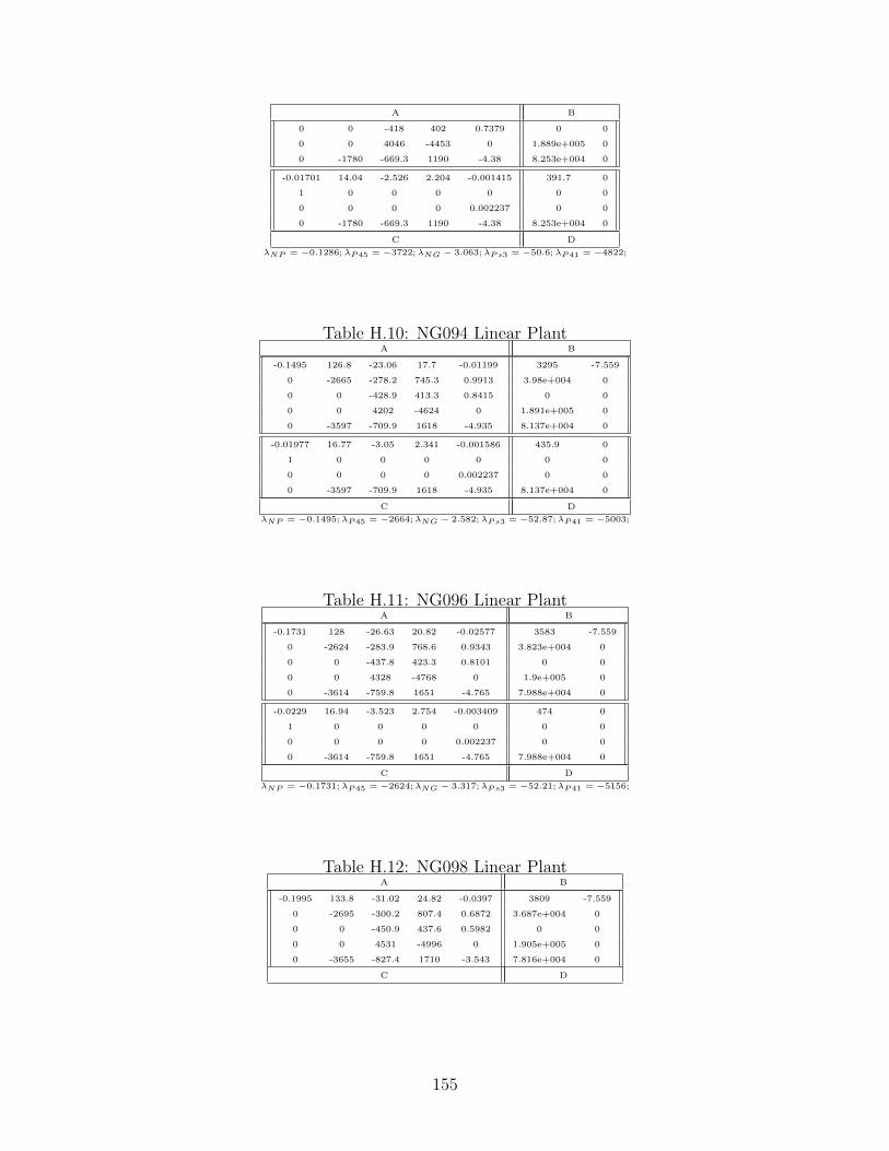
A B
0 0 -418 402 0.7379 0 0
0 0 4046 -4453 0 1.889e+005 0
0 -1780 -669.3 1190 -4.38 8.253e+004 0
-0.01701 14.04 -2.526 2.204 -0.001415 391.7 0
1 0 0 0 0 0 0
0 0 0 0 0.002237 0 0
0 -1780 -669.3 1190 -4.38 8.253e+004 0
C D
λNP = −0.1286;λP45 = −3722;λNG − 3.063;λPs3 = −50.6;λP41 = −4822;
Table H.10: NG094 Linear PlantA B
-0.1495 126.8 -23.06 17.7 -0.01199 3295 -7.559
0 -2665 -278.2 745.3 0.9913 3.98e+004 0
0 0 -428.9 413.3 0.8415 0 0
0 0 4202 -4624 0 1.891e+005 0
0 -3597 -709.9 1618 -4.935 8.137e+004 0
-0.01977 16.77 -3.05 2.341 -0.001586 435.9 0
1 0 0 0 0 0 0
0 0 0 0 0.002237 0 0
0 -3597 -709.9 1618 -4.935 8.137e+004 0
C D
λNP = −0.1495;λP45 = −2664;λNG − 2.582;λPs3 = −52.87;λP41 = −5003;
Table H.11: NG096 Linear PlantA B
-0.1731 128 -26.63 20.82 -0.02577 3583 -7.559
0 -2624 -283.9 768.6 0.9343 3.823e+004 0
0 0 -437.8 423.3 0.8101 0 0
0 0 4328 -4768 0 1.9e+005 0
0 -3614 -759.8 1651 -4.765 7.988e+004 0
-0.0229 16.94 -3.523 2.754 -0.003409 474 0
1 0 0 0 0 0 0
0 0 0 0 0.002237 0 0
0 -3614 -759.8 1651 -4.765 7.988e+004 0
C D
λNP = −0.1731;λP45 = −2624;λNG − 3.317;λPs3 = −52.21;λP41 = −5156;
Table H.12: NG098 Linear PlantA B
-0.1995 133.8 -31.02 24.82 -0.0397 3809 -7.559
0 -2695 -300.2 807.4 0.6872 3.687e+004 0
0 0 -450.9 437.6 0.5982 0 0
0 0 4531 -4996 0 1.905e+005 0
0 -3655 -827.4 1710 -3.543 7.816e+004 0
C D
155
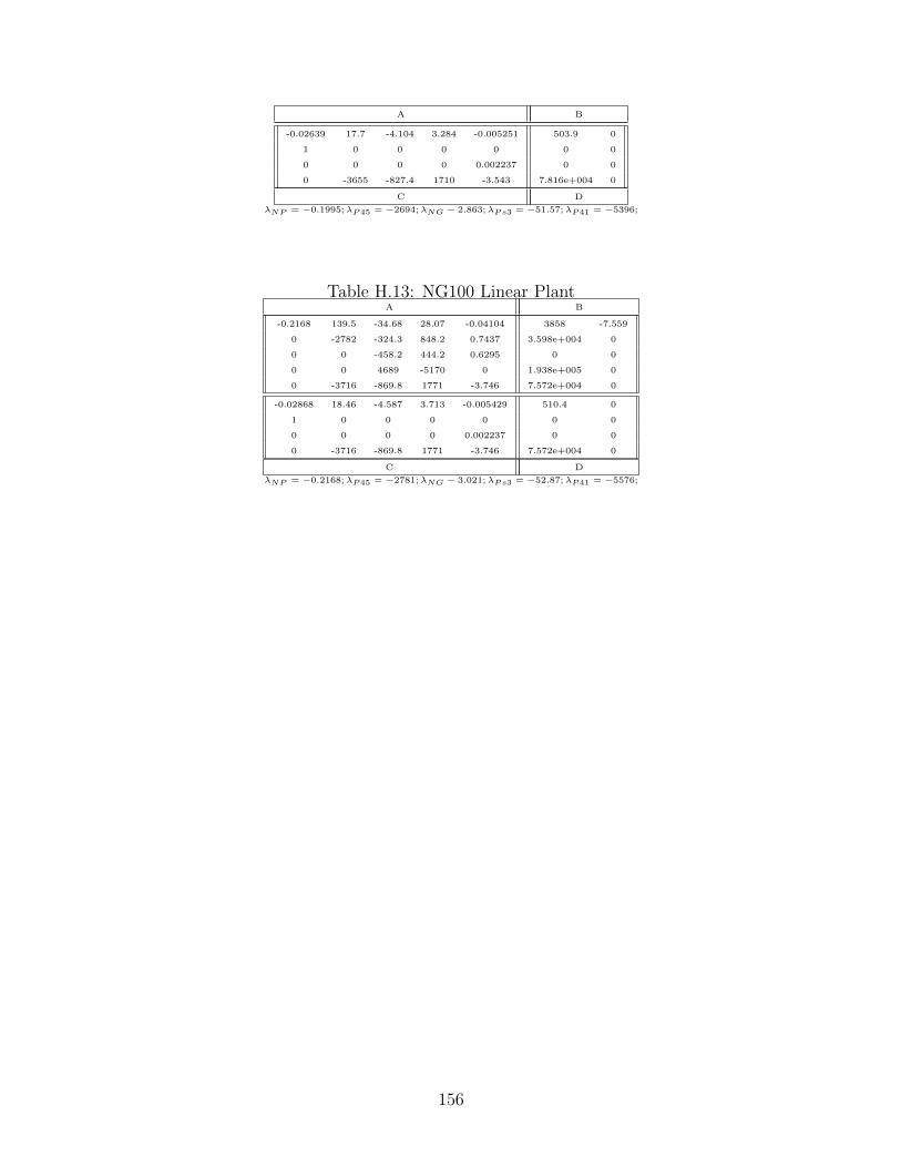
A B
-0.02639 17.7 -4.104 3.284 -0.005251 503.9 0
1 0 0 0 0 0 0
0 0 0 0 0.002237 0 0
0 -3655 -827.4 1710 -3.543 7.816e+004 0
C D
λNP = −0.1995;λP45 = −2694;λNG − 2.863;λPs3 = −51.57;λP41 = −5396;
Table H.13: NG100 Linear PlantA B
-0.2168 139.5 -34.68 28.07 -0.04104 3858 -7.559
0 -2782 -324.3 848.2 0.7437 3.598e+004 0
0 0 -458.2 444.2 0.6295 0 0
0 0 4689 -5170 0 1.938e+005 0
0 -3716 -869.8 1771 -3.746 7.572e+004 0
-0.02868 18.46 -4.587 3.713 -0.005429 510.4 0
1 0 0 0 0 0 0
0 0 0 0 0.002237 0 0
0 -3716 -869.8 1771 -3.746 7.572e+004 0
C D
λNP = −0.2168;λP45 = −2781;λNG − 3.021;λPs3 = −52.87;λP41 = −5576;
156
Bibliography
[1] M. G. Ballin, “A high fidelity real-time simulation of a small turboshaft engine,” NASAAmes Research Center, Moffett Field, CA 94035, July 1998, nASA TM-100991.
[2] P. Gahinet, A. Nemirovski, A. Laub, and M. Chilli, “Manual of LMI control toolbox,”The MathWorks Inc., 1995.
[3] pilotfriend.com. (2010) helicopters: their main components and controls. Copyright:Used with permission. [Online]. Available: http://www.pilotfriend.com/training/flight training/rotary/helis.htm
[4] aerospaceweb.org. (2010) ”turboshaft and turboprop”.Copyright: Used with permission. [Online]. Available: http://www.aerospaceweb.org/question/propulsion/q0209.shtml
[5] Wikipedia:User:Duk. (2006, Mar.) ”file:brayton cycle.svg”. Copyright: Used withpermission under the Creative Commons Attribution ShareAlike 3.0 License. http://creativecommons.org/licenses/by-sa/3.0/. [Online]. Available: http://commons.wikimedia.org/wiki/File:Brayton cycle.svg
[6] W. H. Pfiel, “Multivariable control for the ge t700 engine using the lqr/ltr designmethodology,” Master’s thesis, Department of Mechanical Engineering, Cambridge,July 1984.
[7] M. P. Boyce, Gas Turbine Engineering Handbook - 3rd edition. 30 Corporate Drive,Suite 400, Burlington, MA 01803, USA: Gulf Professional Publishing, 2006.
[8] D. Quattrochi. (2006, Jun.) Brayton cycle. [Online]. Available: http://web.mit.edu/16.unified/www/SPRING/propulsion/notes/node27.html
[9] J. Shamma and M. Athans, “Guaranteed properties of gain scheduled control for linearparameter-varying plants,” Automatica, vol. 27, no. 3, pp. 559–564, 1991.
[10] M. Athans and J. Shamma, “Gain scheduling: Potential hazards and possible reme-dies,” IEEE Control Systems Magazine, vol. 12, pp. 101–107, 1992.
[11] G. Becker and A. Packard, “Robust performance of linear parametrically varyingsystems using parametrically-dependent linear feedback,” Systems & Control Letters,vol. 23, no. 3, pp. 205–215, 1994.
[12] P. Apkarian, P. Gahinet, and G. Becker, “Self-scheduled H∞ control of linearparameter-varying systems: a design example,” Automatica, vol. 31, no. 9, pp. 1251–1261, 1995.
157

[13] R. Sanchez-Pena and M. Sznaier, Robust systems theory and applications, ser. Adaptiveand learning systems for signal processing, communications, and control. John Wiley,1998.
158


