Linear Cosmological Perturbations and Cosmic Microwave...
85
Linear Cosmological Perturbations and Cosmic Microwave Background Anisotropies Carlo Baccigalupi January 21, 2015
Transcript of Linear Cosmological Perturbations and Cosmic Microwave...

Linear Cosmological Perturbations
and
Cosmic Microwave Background Anisotropies
Carlo Baccigalupi
January 21, 2015

2
Contents
1 introduction 7
1.1 things to know for attending the course . . . . . . . . . . . . . . 8
1.2 plan of the lectures . . . . . . . . . . . . . . . . . . . . . . . . . . 9
1.3 notation and micro-elements of general relativity . . . . . . . . . 10
2 Homogeneous and isotropic cosmology 13
2.1 comoving coordinates and conformal time . . . . . . . . . . . . . 14
2.2 stress energy tensor . . . . . . . . . . . . . . . . . . . . . . . . . . 16
2.3 expansion and conservation . . . . . . . . . . . . . . . . . . . . . 16
2.4 relativistic and non-relativistic matter, dark energy . . . . . . . . 17
2.5 brief cosmological thermal history . . . . . . . . . . . . . . . . . . 18
2.6 excercises . . . . . . . . . . . . . . . . . . . . . . . . . . . . . . . 20
2.6.1 question about the dynamics of cosmological abundances 20
2.6.2 question about cosmic acceleration . . . . . . . . . . . . . 20
3 Classification of linear cosmological perturbations 21
3.1 background and perturbation dynamics . . . . . . . . . . . . . . 22
3.2 decomposition of cosmological perturbations in general relativity 23
3.3 Fourier expansion of cosmological perturbations . . . . . . . . . . 25
3.4 perturbations in the metric tensor . . . . . . . . . . . . . . . . . 27
3.4.1 scalar-type components . . . . . . . . . . . . . . . . . . . 27
3.4.2 vector-type components . . . . . . . . . . . . . . . . . . . 28
3.4.3 tensor-type components . . . . . . . . . . . . . . . . . . . 28
3.5 perturbations in the stress energy tensor . . . . . . . . . . . . . . 28
3.5.1 scalar-type perturbations . . . . . . . . . . . . . . . . . . 28
3.5.2 vector-type perturbations . . . . . . . . . . . . . . . . . . 29
3.5.3 tensor-type perturbations . . . . . . . . . . . . . . . . . . 29
3.6 gauge transformations . . . . . . . . . . . . . . . . . . . . . . . . 30
3.6.1 metric tensor transformation . . . . . . . . . . . . . . . . 31
3.6.2 stress energy tensor transformation . . . . . . . . . . . . . 33
3.6.3 gauge dependence, independence, invariance and spuriosity 34
3.7 excercises . . . . . . . . . . . . . . . . . . . . . . . . . . . . . . . 38
3.7.1 question about the cosmological perturbations algebra andmetric tensor fluctuations . . . . . . . . . . . . . . . . . . 38
3.7.2 question about the cosmological perturbations algebra andstress energy tensor fluctuations . . . . . . . . . . . . . . 39
3.7.3 question about gauge invariant formalism . . . . . . . . . 39
3
4 CONTENTS
4 Linear cosmological perturbation dynamics 414.1 analysis of the perturbed einstein and conservation equations . . 42
4.1.1 effective horizon . . . . . . . . . . . . . . . . . . . . . . . 424.1.2 sub-horizon and super-horizon scales . . . . . . . . . . . . 424.1.3 equations for scalar-type perturbations . . . . . . . . . . . 434.1.4 equations for vector-type perturbations . . . . . . . . . . 444.1.5 equations for tensor-type perturbations . . . . . . . . . . 454.1.6 super-horizon evolution . . . . . . . . . . . . . . . . . . . 454.1.7 sub-horizon evolution . . . . . . . . . . . . . . . . . . . . 47
4.2 the Harrison Zel’dovich spectrum . . . . . . . . . . . . . . . . . . 484.3 the power spectrum of matter perturbations today . . . . . . . . 504.4 excercises . . . . . . . . . . . . . . . . . . . . . . . . . . . . . . . 52
4.4.1 question about effective horizon and cosmological scales . 524.4.2 question about density perturbations in a cosmological
constant dominated cosmology . . . . . . . . . . . . . . . 534.4.3 question about the super-horizon scalar-type peculiar ve-
locity . . . . . . . . . . . . . . . . . . . . . . . . . . . . . 534.4.4 question about the Harrison Zel’dovich power spectrum
for gravitational waves . . . . . . . . . . . . . . . . . . . . 534.4.5 question about structure formation in a cosmology which
looks open . . . . . . . . . . . . . . . . . . . . . . . . . . . 54
5 Physics of the cosmic microwave background 555.1 CMB phenomenology . . . . . . . . . . . . . . . . . . . . . . . . 565.2 background and perturbations of a cosmological black body dis-
tribution . . . . . . . . . . . . . . . . . . . . . . . . . . . . . . . . 575.3 polarization . . . . . . . . . . . . . . . . . . . . . . . . . . . . . . 605.4 harmonic decomposition, angular power spectra, and Gaussian
statistics . . . . . . . . . . . . . . . . . . . . . . . . . . . . . . . . 615.4.1 lab−frame . . . . . . . . . . . . . . . . . . . . . . . . . . . 625.4.2 k−frame . . . . . . . . . . . . . . . . . . . . . . . . . . . . 63
5.5 Boltzmann equation . . . . . . . . . . . . . . . . . . . . . . . . . 645.6 gravitational scattering . . . . . . . . . . . . . . . . . . . . . . . . 655.7 Thomson scattering . . . . . . . . . . . . . . . . . . . . . . . . . 675.8 harmonic expansion . . . . . . . . . . . . . . . . . . . . . . . . . 715.9 excercises . . . . . . . . . . . . . . . . . . . . . . . . . . . . . . . 72
5.9.1 question about the dipole Thomson scattering . . . . . . . 72
6 Cosmic microwave background anisotropies 736.1 Solving the Boltzmann equation . . . . . . . . . . . . . . . . . . 746.2 Tight coupling . . . . . . . . . . . . . . . . . . . . . . . . . . . . 776.3 The CMB angular power spectrum . . . . . . . . . . . . . . . . . 78
6.3.1 total intensity . . . . . . . . . . . . . . . . . . . . . . . . . 786.3.2 polarization . . . . . . . . . . . . . . . . . . . . . . . . . . 80
6.4 Relation with cosmological observables . . . . . . . . . . . . . . . 806.5 Status of CMB observation and future expectations . . . . . . . . 806.6 excercises . . . . . . . . . . . . . . . . . . . . . . . . . . . . . . . 80
6.6.1 question about cosmological distances for decoupling . . . 806.6.2 question about angles and scales for the acoustic peaks . 806.6.3 question about the CMB angular power spectrum . . . . 80
CONTENTS 5
6.6.4 question about the role of baryons in acoustic oscillations 816.6.5 question about projection effects for CMB anisotropies . . 826.6.6 question about an integral solution to CMB anisotropies . 826.6.7 question about Silk damping . . . . . . . . . . . . . . . . 83

6 CONTENTS
Chapter 1
introduction
7

8 CHAPTER 1. INTRODUCTION
These are the lecture notes for the course of linear cosmological perturbationsand cosmic microwave background anisotropies for PhD students at SISSA. Overthe years, several students contributed to improve the quality of these notes,with suggestions and corrections. For this, i am thankful to Viviana Acquaviva,Enrico Barausse, Guido D’Amico, Alessandro Lovato, Federico Stivoli.
The aim of these lectures is to describe the physics of the relic radiation incosmology, the Cosmic Microwave Background (CMB), in the framework of thetheory of relativistic linear cosmological perturbations. At the end of the course,a student should be able to understand most of the modern scientific papers onthis matter, ranging from the theoretical details of the CMB anisotropies, downto the physical content and implications of the current experimental data.In this chapter, we give an overview of the course, specifying the most importantliterature to look at, as well as reviewing the plan of the lectures. In the end,we also fix the notation we adopt, and introduce very basic elements of generalrelativity.
1.1 things to know for attending the course
From the point of view of the description of the current cosmological picture,these lectures aim at being self consistent, altough who’s attending might bene-fit from having familiarity with the physics of the Friedmann Robertson Walker(FRW) background cosmology, as well as any knowledge of cosmological per-turbations. Moreover, the physics of the CMB is well known, as at the epochin which it decouples from the other cosmological components, the system wasclose to thermal equilibrium characterized by a temperature of about 3000 K,for instance the same as the external region of a star, and interactions are wellunderstood once the physical constituents are specified.On the other hand, some knowledge of general relativity is necessary in order toapproach these lectures properly. Indeed, the whole cosmology is deeply rootedin general relativity, and with the level of precision of cosmological measure-ments nowadays, getting to the percent or better, it is no longer possible totake Newtonian shortcuts. This is relevant in particular for the whole scheme oflinear cosmological perturbations, which is a most important part of the presentwork.
The main text where studying while attending the course should be repre-sented by these notes. Moreover, the students are welcome to consult the booksand papers which represent the basis of this text. They are:
• textbook by Scott Dodelson, Modern Cosmology, Elsevier Science, 2003,
• review paper by Hideo Kodama and Misao Sasaki, Progresses of Theoret-ical Physics Supplement 78, 1, 1984,
• papers by Wayne Hu and Martin White 1997, Phys. Rev. D 56, 596,Baccigalupi 1999, Phys. Rev. D 59, 123004.
The
• textbook by Andrew R. Liddle and David H. Lyth, Cosmological Inflationand Large Scale Structure, Cambridge Press 2000,
may be also relevant.
1.2. PLAN OF THE LECTURES 9
1.2 plan of the lectures
The first part of the course is dedicated to a summary of the FRW cosmologicalbackground, setting the notation and estabilishing also a continuity with pos-sible previous courses that the students may have attended. The lectures thencover the following topics:
• linear cosmological perturbation theory,
• CMB radiation in cosmology,
• Boltzmann equation for black body radiation in cosmology,
• CMB decoupling and anisotropies, harmonic expansion,
• phenomenology of CMB anisotropies,
• status of CMB observations and the knowledge we have from those up tonow.
The course consists of 14 lectures for the PhD students of the astrophysics andastroparticle courses. The program is the following:
• 1th lecture: introduction and background cosmology (1-2.5),
• 2nd lecture: classification and Fourier expansion of linear cosmologicalperturbations in general relativity (3.1,3.3),
• 3rd lecture: perturbations to the metric and stress energy tensors, gauges(3.4-3.6),
• 4th lecture: gauge transformations and effects (3.6.1-3.6.3),
• 5th lecture: perturbed Einstein and conservation equations (4.1.3-4.1.5),
• 6th lecture: super-horizon evolution (4.1.6),
• 7th lecture: sub-horizon evolution (4.1.7),
• 8th lecture: Harrizon Zel’dovich spectrum (4.2-4.3),
• 9th lecture: CMB physics (5-5.4.2),
• 10th lecture: Boltzmann equation, gravitational and Thomson scattering(5.5-5.8),
• 11th lecture: phenomenology of CMB anisotropies (6-6.2)
• 12th lecture: the obserbed CMB angular power spectrum (6.3-6.3.2),
• 13th lecture: relation with cosmological observables (6.4),
• 14th lecture: status of CMB observations and future expectations (6.5).
The schedule above may undergo variations which will be notified in advance.

10 CHAPTER 1. INTRODUCTION
1.3 notation and micro-elements of general rel-ativity
Spacetime is described by three spatial coordinates plus time. Greek indeces runfrom 0 to 3, while latin indeces are used for spatial dimensions, from 1 to 3. Weuse x to indicate a generic spacetime point, ~x and x for its spatial componentand versor, respectively. The fundamental constants we use are the Boltzmannand Gravitational ones, indicated with kB and G, respectively. We work withunitary velocity of light, c = 1, and Planck constant, ~ = 1.
In general relativity, the infinitesimal distance from two spacetime points isdefined as
ds2 = gµνdxµdxν , (1.1)
where gµν(x) is the metric tensor. By an appropriate change of reference frame,at any given position x it is always possible to reduce the metric tensor to theMinkowski one, meaning that the system changes to the one which is in free falllocally in x. The signature of the metric tensor we adopt is the following:
(−,+,+,+) . (1.2)
Tensors with indeces down are covariant, while the ones with indeces up arecontrovariant. The inverse of the metric tensor is in the controvariant form,and is defined by
gµρgρν = δνµ , (1.3)
where δνµ is the Kronecker delta. We shall use the Kronecker delta in arbitraryindex configuration:
δνµ = δµν = δµν = 1 if µ = ν, 0 otherwise. (1.4)
The Christoffel symbols are defined as usual as
Γαβγ =1
2
(∂gβγ∂xα
+∂gαγ∂xβ
− ∂gαβ∂xγ
),
Γαβγ =1
2gαα
′(∂gα′β∂xγ
+∂gα′γ∂xβ
− ∂gβγ∂xα′
), (1.5)
where the repeated indeces are summed everywhere, unless specified otherwise.The Riemann, Ricci and Einstein tensors are given by
Rαβµν =∂Γαβν∂xµ
−∂Γαβµ∂xν
+ ΓαλµΓλβν − ΓαλνΓλβµ , (1.6)
Rµν = Rααµν , (1.7)
and
Gµν = Rµν −1
2gµνR , (1.8)
where R = Rµµ is the Ricci scalar.To simplify the notation, let us introduce the following conventions for derivationin general relativity:
• ;µ ≡ ∇µ means covariant derivative with respect to xµ,
1.3. NOTATION AND MICRO-ELEMENTS OF GENERAL RELATIVITY11
• |a ≡ γij∇a means covariant derivative with respect to the unperturbedspatial metric in cosmology, γij , defined in (2.4).
• ,µ means ordinary derivative with respect to xµ .
A uni-dimensional tensor, or vector, vµ can be obtained via covariant derivationof a scalar quantity s as
vµ = s;µ = s,µ , (1.9)
where the last equality holds for scalars only. A tensor can be obtained viacovariant derivation of a vector as
tµν = vµ;ν = vµ,ν − vαΓαµν ,
tνµ = vν;µ = vν,µ + vαΓναµ ,
(1.10)
Further covariant derivatives raise the rank of tensors:
uµνρ = tµν;ρ = tµν,ρ − tανΓαµρ − tµαΓαρν
uνµρ = tνµ;ρ = tνµ,ρ − tναΓαµρ + tαµΓνρα . (1.11)
In this way the rank of tensors may be increased at will, keeping the signconventions associated with covariant and controvariant indeces.

12 CHAPTER 1. INTRODUCTION
Chapter 2
Homogeneous and isotropiccosmology
13
14 CHAPTER 2. HOMOGENEOUS AND ISOTROPIC COSMOLOGY
The FRW metric is built upon the hypothesis that there exists a global spa-tial hypersurface orthogonal to the time coordinate at all times, and that spaceis homogeneous and isotropic as seen from any location. Homogeneity meansthat at a given time, the physical properties, e.g. particle number density, veloc-ity, spacetime curvature etc., are the same everywhere in space; isotropy meansthat in addition physical quantities do not depend on the observation direction.These assumptions simplify dramatically the structure of the metric tensor gµν .For orthoginal coordinates, no off-diagonal term is allowed. Moreover, the sys-tem remains with two degrees of freedom only; the first one is a global scalefactor, fixing at each time the value of physical lengths; the second one is relatedto the spacetime curvature, as an homogeneous metric can be globally more orless curved. The form of the fundamental length element may be expressed as
ds2 = −dt2 + a(t)2
(1
1−Kr2dr2 + r2dθ2 + r2 sin2 θdφ2
), (2.1)
where a(t) and K represent the global scale factor and the curvature, respec-tively; r, θ and φ are the usual spherical coordinates for radius, polar angle andangle on the plane orthogonal to the polar direction, respectively.The physical meaning of the scale factor can be read straightforwardly fromthe metric, and the only point to discuss concerns its dimensions. One mayassign physical dimensions to the scale factor a or to the radial coordinate r;in this lectures, we choose the second option. Concerning the curvature, somemore discussion is needed. The first point is about dimensions again; if r isdimensionless, K is also dimensionless. If r is a length, then K is the inverseof the square of a length. Moreover, if K = 0, then the spatial part of thelength (2.1) is Minkowskian, and in this case the FRW metric is defined to beflat. If K > 0, there is a coordinate point in which the metric is singular, givenby rH = ±1/
√K; this means that an infinite physical distance corresponds to
those coordinates, regardless of the value of the scale factor a, and the FRWmetric is defined to be closed; note that this is in agreement with the assump-tion of homogeneity, as this property is the same as seen from all spacetimelocations. If K < 0, the opposite happens, as there is no divergence, and thedistance between two space points vanishes at infinity; in this case the FRWmetric is defined to be open. Finally, note that one may always change theoverall normalization of a or r in (2.1), and therefore, as a pure convention, wecan restrict our attention to three relevant cases for K: for example, if K ischosen to be dimensionless, which is not the case here, K may be chosen to be−1, 0, 1, representing an open, flat and closed FRW cosmology, respectively.
2.1 comoving coordinates and conformal time
Of course one might apply any change of coordinate to the FRW metric, giving itdifferent looks. On the other hand the form (2.1) is the one that is most commonfor cosmological purposes. The reason is that the expansion, represented by thescale factor a, has been factored out of the spatial dependence. This leads us tothe concept of comoving coordinates, i.e. at rest with respect to the cosmologicalexpansion, or in other words defined by the spacetime points for which
r = constant , θ = constant , φ = constant , (2.2)
2.1. COMOVING COORDINATES AND CONFORMAL TIME 15
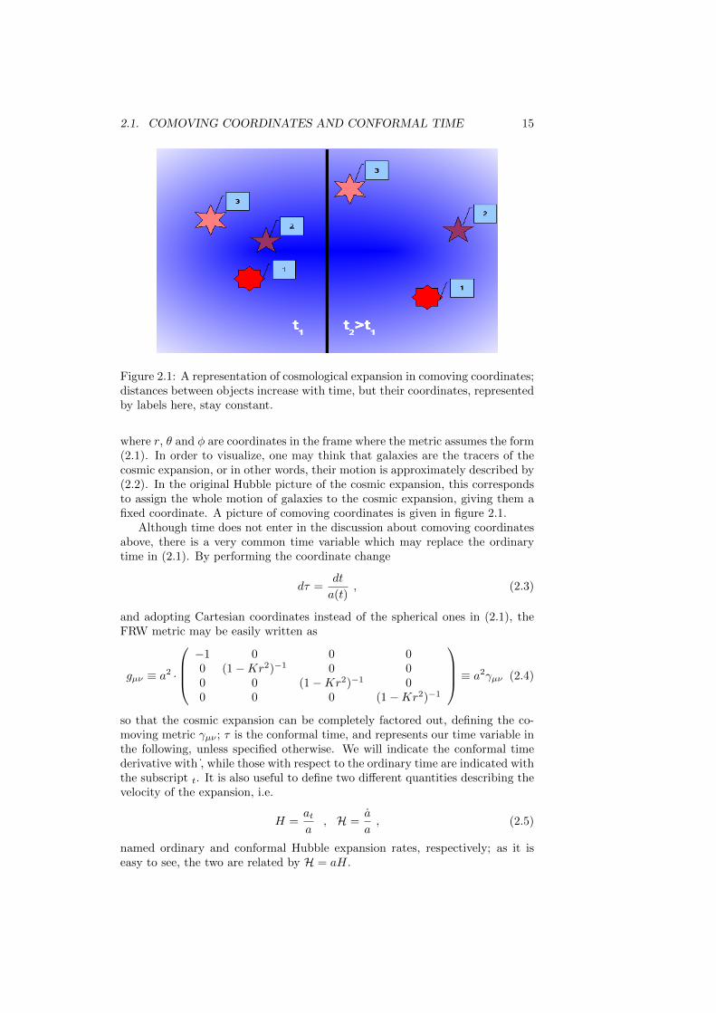
Figure 2.1: A representation of cosmological expansion in comoving coordinates;distances between objects increase with time, but their coordinates, representedby labels here, stay constant.
where r, θ and φ are coordinates in the frame where the metric assumes the form(2.1). In order to visualize, one may think that galaxies are the tracers of thecosmic expansion, or in other words, their motion is approximately described by(2.2). In the original Hubble picture of the cosmic expansion, this correspondsto assign the whole motion of galaxies to the cosmic expansion, giving them afixed coordinate. A picture of comoving coordinates is given in figure 2.1.
Although time does not enter in the discussion about comoving coordinatesabove, there is a very common time variable which may replace the ordinarytime in (2.1). By performing the coordinate change
dτ =dt
a(t), (2.3)
and adopting Cartesian coordinates instead of the spherical ones in (2.1), theFRW metric may be easily written as
gµν ≡ a2 ·
−1 0 0 00 (1−Kr2)−1 0 00 0 (1−Kr2)−1 00 0 0 (1−Kr2)−1
≡ a2γµν (2.4)
so that the cosmic expansion can be completely factored out, defining the co-moving metric γµν ; τ is the conformal time, and represents our time variable inthe following, unless specified otherwise. We will indicate the conformal timederivative with , while those with respect to the ordinary time are indicated withthe subscript t. It is also useful to define two different quantities describing thevelocity of the expansion, i.e.
H =ata
, H =a
a, (2.5)
named ordinary and conformal Hubble expansion rates, respectively; as it iseasy to see, the two are related by H = aH.
16 CHAPTER 2. HOMOGENEOUS AND ISOTROPIC COSMOLOGY
2.2 stress energy tensor
The stress energy tensor specifies the content of spacetime, in terms of physicalentities, i.e. particles and their properties. Here we describe only a perfect rela-tivistic fluid, homogeneous and isotropic. As for the metric, these assumptionsreduce substantially the complexity of the general expression for a stress energytensor. The relevant quantities are just the energy density, ρ, and the pressurep, which need to depend on time only in the FRW background. The stressenergy tensor in the mixed form with covariant and controvariant indeces is indirect relation with ρ and p: the (0, 0) component represent the energy density,while p is isotropically assigned to all directions as
T νµ ≡
−ρ 0 0 00 p 0 00 0 p 00 0 0 p
, (2.6)
where the minus to the energy density is due to the choice of our signature (1.2).The stress energy tensor may also be written as
Tµν = (ρ+ p)uµuν + pgµν , (2.7)
where uµ represents the quadri-velocity of a fluid element with respect to a givenobserver, with an affine parameter which for convenience may be taken as theconformal time itself:
uµ =dxµ
dτ. (2.8)
In analogy with the normalization of the quadri-impulse of a particle with massm, pµp
µ = −m2, the quadri-velocities are the momentum of a unitary massparticle, normalized as uµu
µ = −1. In comoving coordinates, where the ua = 0,this condition implies
uµ ≡(
1
a, 0, 0, 0
). (2.9)
2.3 expansion and conservation
The Einstein and conservation equations
Gµν = 8πGTµν , T;νµν = 0 (2.10)
reduce to two differential equations only, where the independent variable is thetime τ ; they determine the dynamics of the expansion, plus the conservation ofenergy, respectively. The first one is the Friedmann equation
H2 =8πG
3a2ρ−K , (2.11)
which is equivalent to the Ray Choudhury equation describing the accelerationof the expansion:
3H = −4πGa2(ρ+ 3p) . (2.12)
The conservation equation becomes
ρ+ 3H(ρ+ p) = 0 . (2.13)

2.4. RELATIVISTIC ANDNON-RELATIVISTICMATTER, DARK ENERGY17
As it is evident, it is impossible to solve this system if some relation betweenpressure and energy density is given, p(ρ). For interesting cases, as those weshall see in the next Section, pressure is proportional to the energy density:
p = wρ , (2.14)
where w is defined to be the equation of state of the fluid.
2.4 relativistic and non-relativistic matter, darkenergy
So far we did not consider the case in which the stress energy tensor is made bymore than one component, although in realistic conditions, several of those arepresent at the same time. In this case, the stress energy tensor we treated sofar corresponds to the total one, i.e. the sum over those corresponding to eachof the components, labeled by s, as follows:
Tµν =∑s
sTµν . (2.15)
The single stress energy tensors may not be conserved as a result of mutualinteractions between the different species. Therefore, the conservation equationfor each component may be written as
sT;νµν = sQµ , (2.16)
where sQµ represents the non-conservation. Since the total stress energy tensormust be conserved, the interactions between the different components mustsatisfy the condition ∑
s
sQµ = 0 . (2.17)
The simplest example of cosmological component is represented by the non-relativistic (nr) matter. The usual example is that of particles characterized bya temperature giving rise to a thermal agitation which is negligible with respectto the mass m, so that their momentum satisfies the approximation
pµpµ = −m2 ' g00(p0)2 . (2.18)
Whatever the interaction is, in this regime collisions are negligible. No collisionsmeans no pressure, and therefore for this species the equation of state is simplyzero. A most important cosmological component of this kind is commonly knownas Cold Dark Matter (CDM). As it is easy to verify from the conservationequation, the time dependence of this component, assuming that it is decoupledfrom the others, may be expressed as a function of the scale factor as
ρnr ∝ a−3 . (2.19)
The next example is opposite in many respects. Relativistic (r) particles atthermal equilibrium are characterized by an energy which is dominated by ther-mal agitation rather than mass. The condition of thermal equilibrium impliesthat
pr =1
3ρr . (2.20)
18 CHAPTER 2. HOMOGENEOUS AND ISOTROPIC COSMOLOGY
As it is easy to verify from the conservation equation, assuming again that theradiation is not coupled with other species, this implies
ρr ∝ a−4 , (2.21)
which has a direct intuitive meaning. Indeed, taking photons as an example,each of those carries an energy ~ω where ω is the photon frequency, redshiftingwith time as the inverse of the scale factor as a result of the stretching of alllengths. This is responsible for the extra 1/a power in (2.21) with respect to(2.19), which contains only the contribution from the dilution as a result of theexpansion of the volume.A third case, most interesting and dense of theoretical implications, is the casein which the energy density is conserved, i.e.
pde = −ρde , (2.22)
where the subscript means dark energy, which is the class of cosmological specieswhich produces an equation of state close or equal to −1. A constant vacuumenergy density appeared for the first time in the form of a cosmological constantΛ, introduced by Einstein himself in the Einstein equations as a pure geometricalterm:
Gµν + Λgµν = 8πGTµν . (2.23)
Indeed, bringing it to the right hand side, and passing to the mixed form forindeces, one gets
Gνµ = 8πG
(T νµ −
Λ
8πGδνµ
), (2.24)
which shows how a Λ term into the Einstein equation may be interpreted as acomponent of the stress energy tensor. Looking at (2.7) it is straightforward toverify that such component is characterized by pΛ = −ρΛ = −Λ/8πG.
2.5 brief cosmological thermal history
Starting from the Friedmann equation (2.11), it is straightforward to define thecosmological critical density
ρc =3H2
8πG, (2.25)
which allows to write the same equation as
1 =∑s
Ωs , (2.26)
where the cosmological abundance for a given species s is given by
Ωs =ρsρc
, (2.27)
and for consistency the curvature contribution is be also defined as
ΩK = − K
H2. (2.28)
2.5. BRIEF COSMOLOGICAL THERMAL HISTORY 19
Observations in cosmology measure the different abundances. According to themost recent ones (Komatsu et al., 2006), one has
Ωde ' 73% , ΩK ' 0 , Ωnr ' 27% , Ωr ' 10−5 . (2.29)
Since the different components have a different time behavior, as describedin the previous Section, the numbers above change with time. In particular, atearly times, or sufficiently small values of the scale factor, Ωr was larger than theothers, approaching 1 when going indefinitely back in time. The latter conditiondefines the radiation dominated era (RDE); that is followed by one in which thenon-relativistic component dominates, which is called matter dominated era(MDE). At recent times, the expansion is getting dominated by the effect ofthe dark energy. We can give at this point a very brief chronology of the mostrelevant physical processes occurred during these epochs. Given the availableobservations, it is convenient but also reasonable to assume that in the beginningthe universe was mainly characterized by relativistic components only, in mutualthermal equilibrium. This allows to assign a temperature T to the system,corresponding to the temperature of photons, equivalent to an energy scaleE = kBT . The different cosmological species are maintained at equilibrium bytheir physical interactions. The cosmological expansion clearly works againstthe persistence of thermal equilibrium, as it dilutes the density of interactingobjects. One by one, each component decouples from the rest of the system asexpansion proceeds. The last one to decouple is represented by photons, andforms the CMB. Let us review the most important steps in the thermal cosmichistory, going backward in time, up in temperature and energy:
• E ' 10−3 eV, the present epoch of star and galaxy formation and evolution(MDE),
• E ' 10−1 eV, photons decouple from baryons and leptons, origin of theCMB (MDE),
• E ' 100 eV, matter radiation equality,
• E ' 10−1 MeV, nucleosynthesis through deuterium formation from neu-tron proton scattering (RDE),
• E ' 100 MeV, neutrino decoupling from neutrino antineutrino annihila-tion in electron positron pairs, electron positron annihilation in two pho-tons (RDE),
• E ' 102 GeV, symmetry breaking between electromagnetic and weakinteraction (RDE),
• ...?
At higher energies, or earlier cosmological epochs, the electromagnetic and weakinteractions should be described by a single one, named electroweak. Similarmodels exist for the unification of the strong interaction with the others, whichshould occur at earlier cosmological epochs. It is conceivable that also thegravitational interaction unifies with the other forces; although there is nota consensus model for that, one may guess that such epoch corresponds to
20 CHAPTER 2. HOMOGENEOUS AND ISOTROPIC COSMOLOGY
the energy scale which may be formed combining the fundamental constantincluding the gravitational one:
EPlanck =
√~c5G' 1019 GeV . (2.30)
In the above expression, we have momentarily re-introduced the use of the speedof light and Planck constants. If this is indeed the scale at which gravity unifieswith other forces, then a large gap seperates this scale from the highest onewhich may be probed directly in laboratories on the Earth, which is of theorder of the TeV. Cosmology may provide access to relics of early stages in thecosmological history, where typical energy scales were much higher than that.As we will see later in these lectures, the CMB is a typical example, as it carriestraces of the initial cosmological perturbations.
2.6 excercises
2.6.1 question about the dynamics of cosmological abun-dances
The cosmological critical energy density is
ρc =3H2
8πG. (2.31)
Today the ratio between non-relativistic matter energy density and the criticalenergy density, Ωnr 0 = ρnr 0/ρc 0, is about 27%. The same ratio for the darkenergy density is Ωde 0 = ρde 0/ρc 0 = 73%. By describing the dark energy asa Cosmological Constant, pde = −ρde and the non-relativistic matter energydensity as a pressureless component, pnr = 0, find the scale factor ratio of a/a0
for which ρde/ρnr = 103, where a0 is the value of the scale factor today.
2.6.2 question about cosmic acceleration
Assuming that the universe today is described by a flat FRW with dark energyand matter characterized by
Ωde = 73% , Ωnr = 27% , (2.32)
compute the value aa or za = 1/aa−1 at which the acceleration starts, i.e. whena > 0; assume that the dark energy is described as a cosmological constant.In the hypothesis that the universe is completely matter dominated before thatepoch1, compute the cosmological time ta from a = 0 to aa, knowing that theHubble expansion rate today is H0 = 70 km/s/Mpc. Compare the result withthe age of the universe t0 obtained integrating from a = 0 and a = 1, still inthe hypothesis of matter domination.
1Taking into account the radiation dominated era does not lead to substantial changes.
Chapter 3
Classification of linearcosmological perturbations
21
22CHAPTER 3. CLASSIFICATION OF LINEAR COSMOLOGICAL PERTURBATIONS
The whole task we have is to define and understand small perturbationsaround the FRW metric, in a general relativistic framework. The perturbedFRW metric tensor may be defined as
gµν = gµν + δgµν = a2(γµν + hµν) , (3.1)
where the bar means background plus perturbations, i.e. the complete system;hµν(x) represents entirely the perturbation to the metric, and breaks the FRWassumptions completely. We limit our analysis to the linear regime, which maybe simply expressed as
hµν γµν , (3.2)
in any spacetime point x. Note that in a flat FRW background this correspondsto hµν 1. At the same time, the stress energy tensor is perturbed as
T νµ = T νµ + δT νµ , (3.3)
and in this case linearity may be expressed in terms of the non-zero quantitiesin the background tensor, Tµν :
δT νµ ρ, p . (3.4)
One may question what is the motivation for dealing with linear perturbationsonly in cosmology. Indeed, structures we see around us are markedly non-linearin the density distribution, like galaxies or clusters of galaxies. The underlyingassumption is that most of the cosmological evolution occurs in linear regime,while non-linearity is confined to very small scales, reaching the typical sizeof a galaxy or a cluster of galaxies only in cosmologically recent epochs. Agreat support for this assumption comes from the CMB itself. As it is wellknown the CMB temperature anisotropies are at the 10−5 level relatively tothe average temperature over the whole sky, down to an angular resolution ofa few arcminutes. This remarkable level of isotropy suggests that the densityfluctuations, and cosmological perturbations in general, were in a linear regimeat the epoch in which the CMB radiation decoupled from the rest of the system.Then, the linear approximation should be valid to describe the bulk of physicalcosmology on a large interval of time and physical scales, before and after theCMB origin, breaking down only recently and on scales smaller than those ofgalaxy clusters.
3.1 background and perturbation dynamics
Linearity allows to neglect the terms of second or higher orders, i.e. involvingproducts of fluctuations. A direct consequence of this concerns the relativisticalgebra of cosmological perturbations. Of course, in a perturbed FRW environ-ment, tensor indeces are raised and lowered using the complete metric, gµν . Onthe other hand, linearity allows to neglect the second or higher order terms. Thisimplies non-trivial relations between fluctuations with different configurationsof indeces. By using the usual general relativistic relation gµν = gµµ
′gνν
′gµ′ν′
one gets
δgµν = −gµµ′gνν
′δgµ′ν′ , (3.5)
3.2. DECOMPOSITION OF COSMOLOGICAL PERTURBATIONS IN GENERAL RELATIVITY23
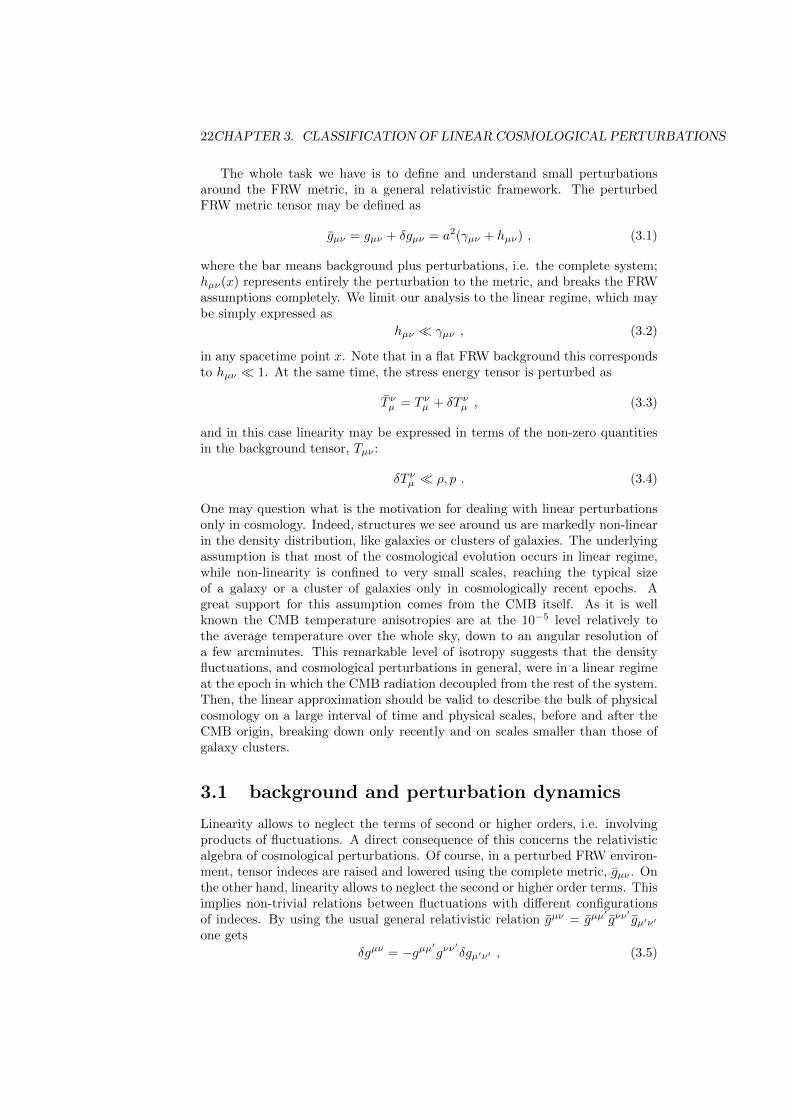
Figure 3.1: A representation of scalar-type (left) and vector-type (right) vectorfields.
where we used the fact that the background metric is diagonal. Another, mostimportant consequence of the linear scheme is that the background dynamicsis not influenced by perturbations:the prescription is no longer valid wheneverhµν approaches unity or δT νµ gets close to the background energy density orpressure. Therefore, any equation in cosmology splits in two, concerning thebackground and perturbation dynamics, respectively:
Gµν = 8πGTµν ≡
Gµν = 8πGTµνδGµν = 8πGδTµν
, (3.6)
T ;νµν = 0 ≡
T ;νµν = 0
δ(T ;νµν) = 0
. (3.7)
Note that, on the contrary, perturbations are affected by the background dy-namics. The scale factor evolution, as well as the dynamics of energy densityand pressure, do appear explicitely in the perturbation equations, as we shallsee in the following.
3.2 decomposition of cosmological perturbationsin general relativity
We now carry out a general discussion concerning the different components ofthe cosmological perturbations, hµν and δTµν . This is done on the basis oftheir physical properties in a general relativistic framework, yielding a simplebut general classification, which is one of the basis of modern cosmology. Thefluctuations depend on the spacetime point x ≡ (τ, ~x). The decompositionis made considering the spatial part only, while the perturbed Einstein andconservation equations (3.6, 3.7) give the time dependence of each species.Let us consider in general the space dependence of functions in general relativity,but restricting ourselves to the spatial metric at a fixed time, γij . Under spatialrotations, a function of the space may behave as a scalar, vector or tensor:
s(~x) , vi(~x) , tij(~x) . (3.8)
While the physical nature of scalars is unique, the classification gets non-trivialalready for vectors. Indeed, each vector function may be divided in full general-ity in a part which may be obtained via derivation of a scalar, and the rest. The
24CHAPTER 3. CLASSIFICATION OF LINEAR COSMOLOGICAL PERTURBATIONS
first component is called scalar-type component of the vector, while the secondone is called vector-type component of the vector. In a similar way, tensorsmay be divided in three components. The first one, called scalar-type compo-nent, comes from double derivation of a scalar function. The second one, calledvector-type component, comes from derivation of a vector-type component ofa vector. The remaining part is called tensor-type component. Technically, byderivation here we mean the covariant one with respect to the γij metric, as weare still in a general relativistic framework, even if the FRW assumptions areallowing us to restrict ourselves to space. Let us see all that in formulas now.For vectors, one has
vi = s|i + vi∗ , (3.9)
indicating scalar-type and vector-type components, respectively; mathemati-cally, the relation above is also known as the Helmholtz equation. Still main-tining full generality, s may be chosen is such in order to be responsible for thedivergence of the whole vector function:
γijs ≡ s|i|i = vi|i = v . (3.10)
This implies that the vector-type component is divergenceless:
vi∗|i = 0 . (3.11)
As we will see in a moment, this has a direct and intuitive physical meaning.For tensors, the decomposition may be written as
tij = s|ij + vi|j∗ + tij∗ . (3.12)
In analogy with what has been done for vectors, in general the scalar-typecomponent is responsible for the trace of the tensor, obeying the equation
γijs = tii ≡ t , (3.13)
while the vector-type is divergenless and obeys the same condition as in (3.11).This implies that the tensor-type component is traceless:
ti∗i = 0 . (3.14)
We may further restrict the properties of tij∗ . The divergence of tij is given by
tij|j = s|ij|j + v
i|j∗|j + tij∗|j . (3.15)
Within the constraint on s given by (3.13), we may require in full generalitythat the vector-type component satisfies
vi|j∗|j = tij|j − s
|ij|j , (3.16)
which implies
t|j∗ij = 0 . (3.17)
The relations (3.17,3.14), together with the one above, are known as the trans-verse traceless conditions, respectively.The physical interpretation of this decomposition is rather simple. Consider for
3.3. FOURIER EXPANSION OF COSMOLOGICAL PERTURBATIONS 25
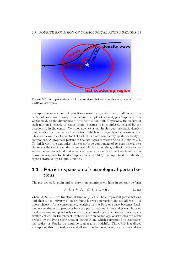
Figure 3.2: A representation of the relation between angles and scales in theCMB anisotropies.
example the vector field of velocities caused by gravitational infall toward thecenter of some overdensity. That is an example of scalar-type component of avector field, as the divergence of this field is non-null. Physically, the nature ofsuch motion is clearly of scalar origin, because it is completely caused by theoverdensity in the center. Consider now a vortex. In this case, no static densityperturbation can cause such a motion, which is divergenless by construction.This is an example of a vector field which is made completely by its vector-typecomponent. A graphical picture of the two types of vector fields is in figure 3.1.To finish with the examples, the tensor-type component of tensors describe tothe tensor fluctuation modes in general relativity, i.e. the gravitational waves, aswe see below. As a final mathematical remark, we notice that the classificationabove corresponds to the decomposition of the SO(3) group into its irreduciblerepresentations, up to spin 2 modes.
3.3 Fourier expansion of cosmological perturba-tions
The perturbed Einstein and conservation equations will have in general the form
A · δ1 +B · δ2 + C · δ3 + ... = 0 , (3.18)
where A,B,C, ... are function of time only, while the δi represent perturbationsand their time derivatives; no products between perturbations are allowed in alinear theory. As a consequence, working in the Fourier space becomes feasi-ble, as the absence of products between perturbed quantities makes each Fouriermode evolving independently on the others. Working in the Fourier space is par-ticularly useful in the present context, since in cosmology observables are oftenprobed by studying their angular distribution, which correspond to cosmolog-ical scales, or Fourier wavenumbers, at a given redshift. The CMB is a directexample of this. Indeed, as we shall see, the last scattering is a rather sudden
26CHAPTER 3. CLASSIFICATION OF LINEAR COSMOLOGICAL PERTURBATIONS
event in cosmology, and the thickness of the last scattering surface would corre-spond today to a distance of about 10 Mpc, compared with almost 10000 Mpcfrom us. The angular distribution of CMB anisotropies directly corresponds toits Fourier expansion, expecially on small angular scales. This is graphicallyrepresented in figure 3.2. In this Section, therefore, we lay down the formalismnecessary to study cosmological perturbations in the Fourier space, and thatwill be our framework in the following.
We expand perturbations into a complete set of functions which are theeigenfunctions of the Laplace Beltrami operator γijf = γijf|ij . For scalarfunctions, those eigenfunctions Y~k(~x) are the solutions of the differential equa-tion
(γij + k2)Y = 0 . (3.19)
where k = |~k| and we drop the explicit arguments of Y~k(~x) in the following. Notethat in flat cosmology γij is just the Laplacian operator, and the solutions ofthe equation above are just plane waves:
Y ∝ ei~k·~x in flat FRW . (3.20)
The scalar-type components of vectors is expanded in Fourier modes exploitingthe simple derivation of the functions above, expressed as
Yi = −1
kY|i , (3.21)
where the factor and sign in front are purely conventional. Similarily, the scalar-type component of tensors may be expanded in the following Fourier modes:
Yij =1
k2Y|ij +
1
3γijY . (3.22)
From (3.19) note that the expression above is traceless; indeed it will be conve-nient to express the trace of tensors separately.The vector-type component of vectors may be expanded into the vector solutionsof the Laplace Beltrami operator, i.e. obeying
(γij + k2)Y(±1)i = 0 , (3.23)
with the divergenceless constraint
γijY(±1)i|j = 0 , (3.24)
and the ±1 symbol indicates that there exist two independent solutions satis-fying the divergenceless constraint. The vector-type component of tensors maybe expanded into
Y(±1)ij = − 1
2k
(Y
(±1)i|j + Y
(±1)j|i
), (3.25)
where the sum is made in order to describe symmetric quantities like elementsin the metric tensor are.Finally, the tensor-type component of tensors may be expanded into the tensorsolutions of the Laplace Beltrami operator
(γij + k2)Y(±2)ij = 0 , (3.26)
3.4. PERTURBATIONS IN THE METRIC TENSOR 27
with the transverse traceless constraint
Y(±2)|jij = 0 = Y
(±2)ii , (3.27)
and as above the ±2 symbol indicates that there exist two independent solutionssatisfying the transverse traceless constraint. From now on, we adopt the Fourierspace as our default framework, working out the analysis for one generic mode;as already mentioned, unless otherwise specified, we drop the label ~k.
3.4 perturbations in the metric tensor
We have now all the necessary tools to define and classify the different speciesof cosmological perturbations in general relativity. The classification is entirelydone in terms of the properties under spatial rotations of the perturbation com-ponents, defined in section 3.2, and we consider those of the metric tensor first,δgµν ; with the addition of the background component, they represent the to-tal metric tensor (3.1), gµν = gµν + δgµν . We choose to work in Cartesiancoordinates, where from (2.4) the background non-zero terms are g00 = −a2,g11 = a2/(1−Kr2) = g22 = g33. We consider δgµν and define scalar and scalar-type components, vector and vector-type components, tensor and tensor-typecomponents, respectively.
3.4.1 scalar-type components
The δg00 quantity is clearly a scalar, since it does not contain any spatial index.In the Fourier space, it may be defined as
δg00 = −2a2AY , (3.28)
where A and Y represent the Fourier amplitude and Laplace Beltrami operatoreigenfunction at wavenumber ~k, respectively. As we already mentioned, unlessspecified otherwise we do not indicate the arguments τ in a, τ and ~k in A, ~k and~x in Y , as in the following those dependences remain the same for all backgroundterms, perturbations and Fourier eigenfunctions, respectively. Obviously, at anytime the real space expression of the perturbations in the Fourier space may begot as follows:
δg00(τ, ~x) =
∫d3k
(2π)3A(τ,~k)Y (~k, ~x) . (3.29)
The quantity δg0i is a vector, and since the background term for that is zero,it coincides with the component of the total metric tensor, g0i. Just like anyvector in our scheme, it contains scalar-type and vector-type components. Itsscalar-type component may be defined as
δg0i = −a2BYi . (3.30)
The quantity δgij contains scalar-type components on the diagonal, also yieldinga perturbation in its trace, plus vector-type and tensor-type traceless contribu-tions. The scalar-type component may be written as
δgij = 2a2(HLY γij +HTYij) , (3.31)
28CHAPTER 3. CLASSIFICATION OF LINEAR COSMOLOGICAL PERTURBATIONS
where HL and HT represent the amplitude at the Fourier mode ~k of the diagonal(L stays for longitudinal) and non-diagonal (T stays for transverse) componentsof the perturbations to the metric tensor. Indeed, in the mixed form the secondterm in the right hand side appears simply as 2HLY δ
ji , and Yij is traceless as
it is evident from (3.22). The transverse component, which as we see now hasvector and tensor-type components as well, is also known as shear in the metric.
3.4.2 vector-type components
In analogy with (3.30), we may define the vector-type contribution to the metrictensor fluctuation as
δg(±1)0i = −a2B(±1)Y
(±1)i . (3.32)
The vector-type contribution to δgij does not possess the trace part, reducingto the shear component only, which we may write as
δg(±1)ij = 2a2H
(±1)T Y
(±1)ij , (3.33)
representing the vector-type component of the metric shear.
3.4.3 tensor-type components
The tensor-type fluctuations in the metric has only a shear component, and maybe written as
δg(±2)ij = 2a2H
(±2)T Y
(±2)ij . (3.34)
This term represents the Fourier amplitude of cosmological gravitational waves,corresponding to the transverse traceless perturbation component.
3.5 perturbations in the stress energy tensor
It is convenient to work with the indeces in the mixed form, as they have a directphysical meaning, e.g. represent energy density, pressure, momentum densityetc.. As for the metric tensor, the total stress energy tensor may be written asin (3.3), where the background non-zero contributions are T 0
0 = −ρ, T 11 = T 2
2 =T 3
3 = p. If different components are present in the stress energy tensor, theirperturbations are still characterized by the quantities defined below, each onelabeled with a species index s.
3.5.1 scalar-type perturbations
The perturbation component of T 00 concerns the energy density distribution.
We may write it as
δT 00 = −ρδY , (3.35)
introducing the Fourier amplitude of the spatial fluctuations in the density con-trast, δ(τ,~k) ≡ δρ(τ,~k)/ρ(τ). Similarily, the perturbed momentum concideswith the corresponding component of the total stress energy tensor T i0 and isexpressed as
δT i0 = (ρ+ p)vY i , (3.36)
3.5. PERTURBATIONS IN THE STRESS ENERGY TENSOR 29
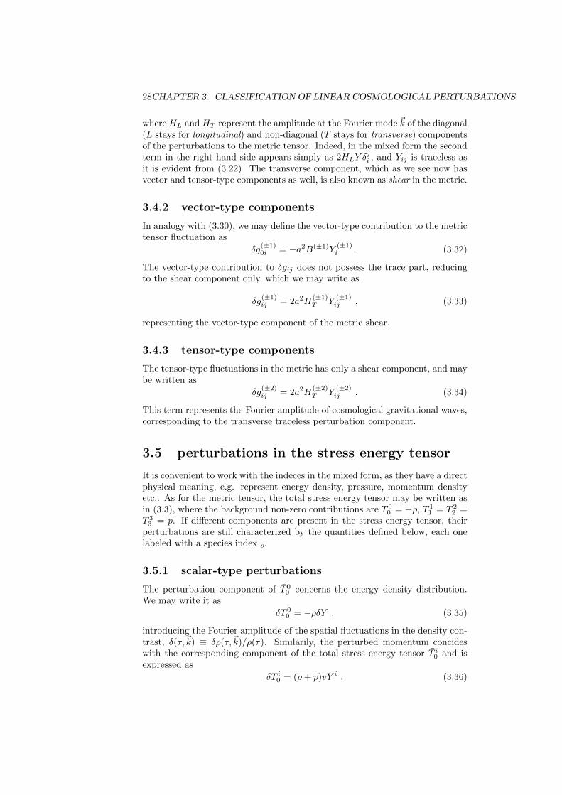
Figure 3.3: A representation of rotation and boost gauge transformations, inthe left and right panel, respectively; in the two frames, both linearly close tothe FRW one, the cosmological perturbations represented as the ball appearsto have different coordinate location and peculiar velocity, respectively.
where v represents the peculiar velocity, i.e. the velocity component with whichthe perturbed fluid drifts away from the Hubble flow, and ρ+p gives the effectivemomentum mass. Finally, the scalar-type stress energy perturbations are madeby an isotropic or trace part, plus the traceless component, commonly knownas shear, given by
δT ji = p(πLY δji + πTY
ji ) , (3.37)
where the first component, πL (as for the metric L means longitudinal) maybe seen as the Fourier amplitude of the perturbation to the pressure contrast,πL(τ,~k) ≡ δp(τ,~k)/p(τ), in analogy with what has been done for the energydensity. The other component, πT (where again T means transverse), representsthe stress energy shear component, as we see now has vector and tensor-typecomponents as well.
3.5.2 vector-type perturbations
In analogy with the definitions (3.36) and (3.37), but dealing with the vector-type components, we may write
δTi(±1)0 = (ρ+ p)v(±1)Y i(±1) , (3.38)
δTj(±1)i = pπ
(±1)T Y
j(±1)i , (3.39)
which represent the vector-type contributions to the perturbed stress energy
tensor; v(±1) may be seen as the Fourier amplitude of vorticity, while π(±1)T is
the shear of vector-type origin.
3.5.3 tensor-type perturbations
Finally, tensor-type perturbations affect the shear component only, and we maywrite those as
δTj(±2)i = pπ
(±2)T Y
j(±2)i , (3.40)
which represent the stress energy counterpart of the gravitational waves H(±2)T
defined in (3.34).
30CHAPTER 3. CLASSIFICATION OF LINEAR COSMOLOGICAL PERTURBATIONS
3.6 gauge transformations
As we have seen so far, the linearization of general relativity yields a quite sim-ple decomposition of the different contributions on the basis of their geometricalproperties. Linearity implies that in the Einstein equations no terms involvingthe product of two or more perturbations are considered, and that the equationsthemselves split in two sub-sets, one evolving the cosmological background, andone dealing with the perturbation evolution. In other words, linearization cre-ates a new set of dynamical variables, the small perturbations around the FRWbackground, which are obviously not built-in general relativity. Of course, lin-ear perturbations are different in different frames, and in particular on thosediffering by small amounts from the Hubble frame where the background metricis given by (2.4), yielding effects comparable to the perturbations themselves.Those frames are called gauges. The coordinate transformations between dif-ferent gauges, involving coordinate shifts of the same order of the perturbationsthemselves, determine how the perturbed quantities in different gauges are re-lated. We indicate gauge transformations as
xµ = xµ + δxµ(x) , (3.41)
where δxµ, function of the spacetime point x, represents the coordinate shiftbetween the new frame labeled with f , and the original one, f .Cosmological perturbations appear different in different gauges, as shown infigure 3.3 for a small rotation and boost, making a perturbation representedas a ball having different coordinate locations and velocity, respectively. Atypical example of the second case is represented by the cosmological dipole,i.e. the dipole term in the angular expansion of the CMB temperature which isattributed to a Doppler shift due to the local motion, represented by a peculiarvelocity ~v of our group of galaxies; the perturbation to the CMB temperature,and consequently our velocity, is measured to be rather small in units of thelight velocity, so that the arguments of linear cosmological perturbation theorymay be applied: (
δT
T
)dipole
= v ' 10−3 . (3.42)
Indeed, in a frame moving with velocity −~v with respect to our local group ofgalaxies, no dipole would be seen. That is an example of gauge transformation,as the velocity shift is small as in (3.42). This example tells us two importantaspects. First, cosmological perturbations, represented here by the CMB tem-perature, do depend on the chosen gauge. Second, perturbations may be zero insome gauges, and non-zero in others. We now treat more formally these issues.The coordinate shifts δxµ are functions of the spacetime point x and obey thesame classification as we did in section 3.2:
δx0 is a scalar function, (3.43)
δxi is a vector function, (3.44)
composed by scalar-type and a vector-type components. We will express thegauge transformation laws in the Fourier space, therefore it is convenient to
3.6. GAUGE TRANSFORMATIONS 31
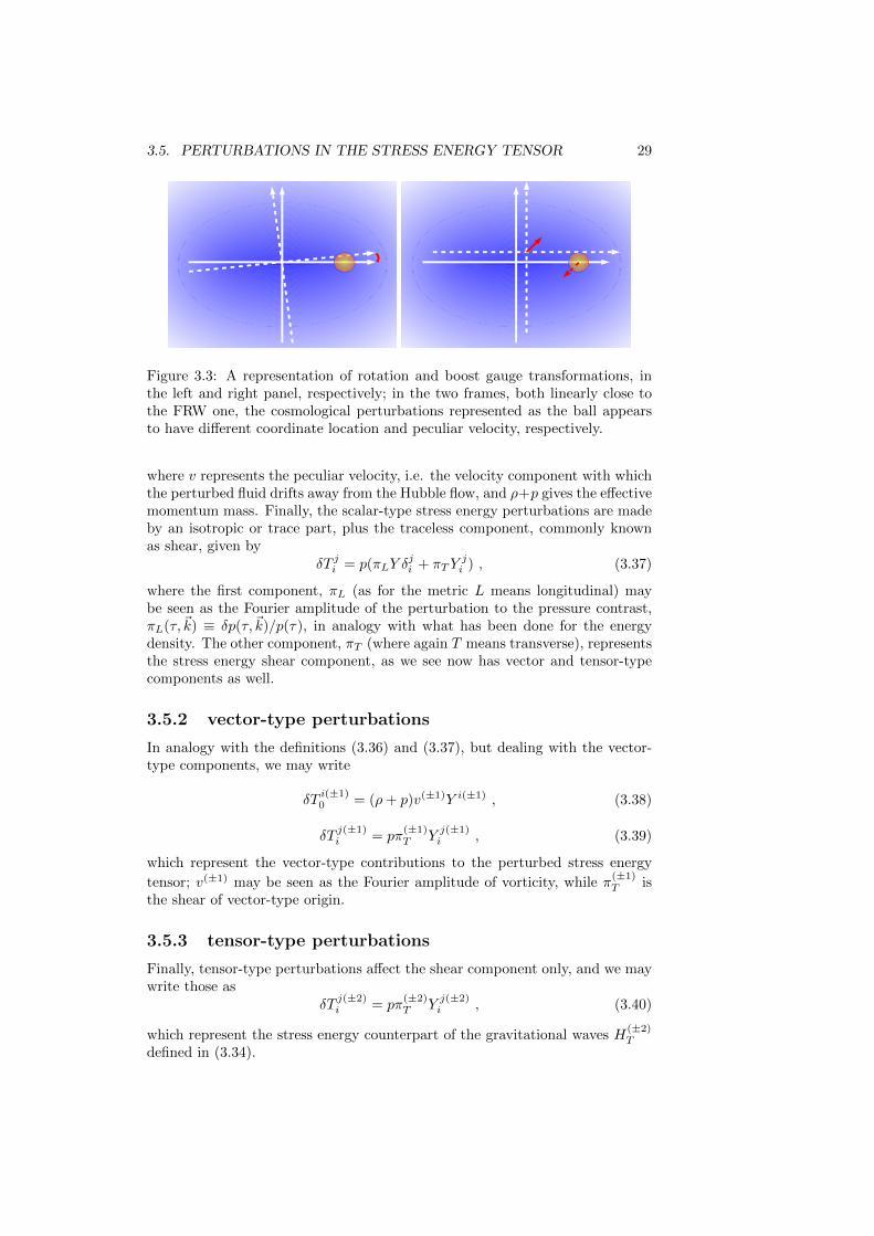
Figure 3.4: A representation of the Doppler shift on CMB photons, representedas γs, caused by our own peculiar motion with respect to the one where theCMB dipole is absent.
define the Fourier amplitudes of δxµ:
δx0(τ, ~x) =
∫d3k
(2π)3T (τ,~k)Y (~k, ~x)
δxi(τ, ~x) =
∫d3k
(2π)3[L(τ,~k)Y i(~k, ~x) + L(±1)(τ,~k)Y i(±1)(~k, ~x)] . (3.45)
Again we do not indicate explicitely the arguments of the functions T , L, L(±1)
in the following. To find how perturbed quantities transform under gauge trans-formations it is enough to use the transformation laws of tensors in general rel-ativity, keeping the linear order both in the perturbations and in the coordinateshifts as well, as we show now.
3.6.1 metric tensor transformation
The general transformation of gµν between f and f is
gµν(x) =∂xµ
′
∂xµ∂xν
′
∂xν˜gµ′ν′(x) , (3.46)
where as usual the bar means background plus perturbations. It is easy toexpress the partial derivatives above as a function of the shifts δxµ:
∂xµ′
∂xµ= δµ
′
µ + δxµ′
,µ ,∂xν
′
∂xν= δν
′
ν + δxν′
,ν . (3.47)
By keeping only the first order terms in the shifts, from (3.46) one obtains
gµν(x) = ˜gµν(x) + ˜gµ′ν(x)δxµ′
,µ + ˜gµν′(x)δxν′
,ν . (3.48)
To solve the relation above and find the transformation laws between pertur-bations, we need to express all quantities above in the same coordinate point.
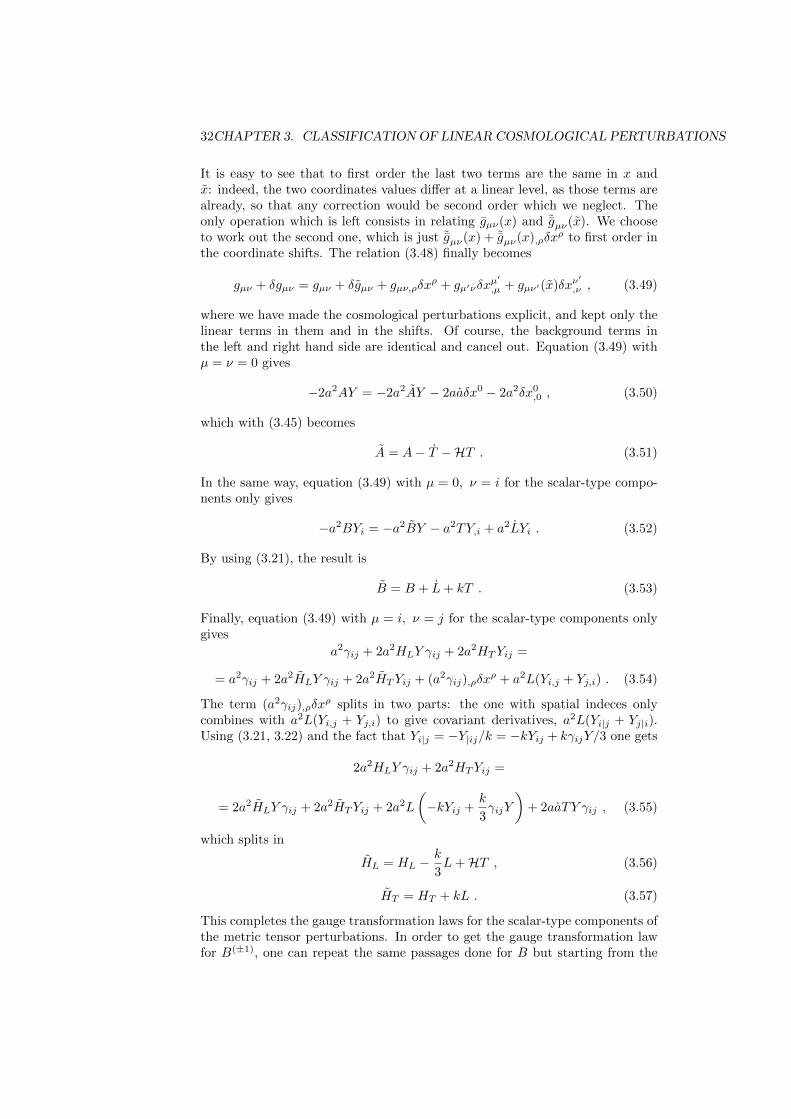
32CHAPTER 3. CLASSIFICATION OF LINEAR COSMOLOGICAL PERTURBATIONS
It is easy to see that to first order the last two terms are the same in x andx: indeed, the two coordinates values differ at a linear level, as those terms arealready, so that any correction would be second order which we neglect. Theonly operation which is left consists in relating gµν(x) and ˜gµν(x). We chooseto work out the second one, which is just ˜gµν(x) + ˜gµν(x),ρδx
ρ to first order inthe coordinate shifts. The relation (3.48) finally becomes
gµν + δgµν = gµν + δgµν + gµν,ρδxρ + gµ′νδx
µ′
,µ + gµν′(x)δxν′
,ν , (3.49)
where we have made the cosmological perturbations explicit, and kept only thelinear terms in them and in the shifts. Of course, the background terms inthe left and right hand side are identical and cancel out. Equation (3.49) withµ = ν = 0 gives
−2a2AY = −2a2AY − 2aaδx0 − 2a2δx0,0 , (3.50)
which with (3.45) becomes
A = A− T −HT . (3.51)
In the same way, equation (3.49) with µ = 0, ν = i for the scalar-type compo-nents only gives
−a2BYi = −a2BY − a2TY,i + a2LYi . (3.52)
By using (3.21), the result is
B = B + L+ kT . (3.53)
Finally, equation (3.49) with µ = i, ν = j for the scalar-type components onlygives
a2γij + 2a2HLY γij + 2a2HTYij =
= a2γij + 2a2HLY γij + 2a2HTYij + (a2γij),ρδxρ + a2L(Yi,j + Yj,i) . (3.54)
The term (a2γij),ρδxρ splits in two parts: the one with spatial indeces only
combines with a2L(Yi,j + Yj,i) to give covariant derivatives, a2L(Yi|j + Yj|i).Using (3.21, 3.22) and the fact that Yi|j = −Y|ij/k = −kYij + kγijY/3 one gets
2a2HLY γij + 2a2HTYij =
= 2a2HLY γij + 2a2HTYij + 2a2L
(−kYij +
k
3γijY
)+ 2aaTY γij , (3.55)
which splits in
HL = HL −k
3L+HT , (3.56)
HT = HT + kL . (3.57)
This completes the gauge transformation laws for the scalar-type components ofthe metric tensor perturbations. In order to get the gauge transformation lawfor B(±1), one can repeat the same passages done for B but starting from the
3.6. GAUGE TRANSFORMATIONS 33
vector-type component of equation (3.49) with µ = 0, ν = i, not consideringthe term involving T as that is a scalar-type quantity:
B(±1) = B(±1) + L(±1) . (3.58)
In the same way, the gauge transformation laws for H(±1)L and H
(±1)T can be
obtained repeating the same passages done for HL and HT but starting fromthe vector-type component of equation (3.49) with µ = i, ν = j, not consideringthe term involving T as that is a scalar-type quantity:
H(±1)L = H
(±1)L − k
3L(±1) , (3.59)
H(±1)T = H
(±1)T + kL(±1) . (3.60)
Finally, a most important consideration is that since gauge transformations maybe scalar-type or vector-type only, any tensor-type cosmological perturbation isgauge invariant.
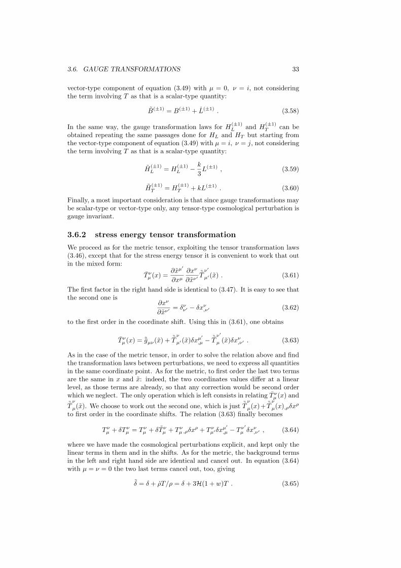
3.6.2 stress energy tensor transformation
We proceed as for the metric tensor, exploiting the tensor transformation laws(3.46), except that for the stress energy tensor it is convenient to work that outin the mixed form:
T νµ (x) =∂xµ
′
∂xµ∂xν
∂xν′˜Tν′
µ′(x) . (3.61)
The first factor in the right hand side is identical to (3.47). It is easy to see thatthe second one is
∂xν
∂xν′= δνν′ − δxν,ν′ (3.62)
to the first order in the coordinate shift. Using this in (3.61), one obtains
T νµ (x) = ˜gµν(x) + ˜Tν
µ′(x)δxµ′
,µ − ˜Tν′
µ (x)δxν,ν′ . (3.63)
As in the case of the metric tensor, in order to solve the relation above and findthe transformation laws between perturbations, we need to express all quantitiesin the same coordinate point. As for the metric, to first order the last two termsare the same in x and x: indeed, the two coordinates values differ at a linearlevel, as those terms are already, so that any correction would be second orderwhich we neglect. The only operation which is left consists in relating T νµ (x) and˜Tν
µ(x). We choose to work out the second one, which is just ˜Tν
µ(x)+ ˜Tν
µ(x),ρδxρ
to first order in the coordinate shifts. The relation (3.63) finally becomes
T νµ + δT νµ = T νµ + δT νµ + T νµ ,ρδxρ + T νµ′δx
µ′
,µ − T ν′
µ δxν,ν′ , (3.64)
where we have made the cosmological perturbations explicit, and kept only thelinear terms in them and in the shifts. As for the metric, the background termsin the left and right hand side are identical and cancel out. In equation (3.64)with µ = ν = 0 the two last terms cancel out, too, giving
δ = δ + ρT/ρ = δ + 3H(1 + w)T . (3.65)
34CHAPTER 3. CLASSIFICATION OF LINEAR COSMOLOGICAL PERTURBATIONS
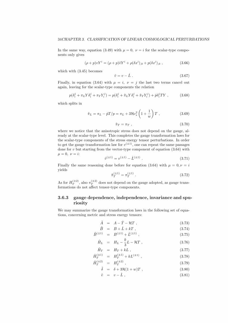
In the same way, equation (3.49) with µ = 0, ν = i for the scalar-type compo-nents only gives
(ρ+ p)vY i = (ρ+ p)vY i + ρ(δxi),0 + p(δxi),0 , (3.66)
which with (3.45) becomesv = v − L . (3.67)
Finally, in equation (3.64) with µ = i, ν = j the last two terms cancel outagain, leaving for the scalar-type components the relation
p(δji + πLY δji + πTY
ji ) = p(δji + πLY δ
ji + πTY
ji ) + pδji TY , (3.68)
which splits in
πL = πL − pT/p = πL + 3Hc2s(
1 +1
w
)T , (3.69)
πT = πT , (3.70)
where we notice that the anisotropic stress does not depend on the gauge, al-ready at the scalar-type level. This completes the gauge transformation laws forthe scalar-type components of the stress energy tensor perturbations. In orderto get the gauge transformation law for v(±1), one can repeat the same passagesdone for v but starting from the vector-type component of equation (3.64) withµ = 0, ν = i:
v(±1) = v(±1) − L(±1) . (3.71)
Finally the same reasoning done before for equation (3.64) with µ = 0, ν = iyields
π(±1)T = π
(±1)T . (3.72)
As for H(±2)T , also π
(±2)T does not depend on the gauge adopted, as gauge trans-
formations do not affect tensor-type components.
3.6.3 gauge dependence, independence, invariance and spu-riosity
We may summarize the gauge transformation laws in the following set of equa-tions, concerning metric and stress energy tensors:
A = A− T −HT , (3.73)
B = B + L+ kT , (3.74)
B(±1) = B(±1) + L(±1) , (3.75)
HL = HL −k
3L−HT , (3.76)
HT = HT + kL , (3.77)
H(±1)T = H
(±1)T + kL(±1) , (3.78)
H(±2)T = H
(±2)T , (3.79)
δ = δ + 3H(1 + w)T , (3.80)
v = v − L , (3.81)
3.6. GAUGE TRANSFORMATIONS 35
v(±1) = v(±1) − L(±1) , (3.82)
πL = πL + 3Hc2s(
1 +1
w
)T , (3.83)
πT = πT , (3.84)
π(±1)T = π
(±1)T , (3.85)
π(±2)T = π
(±2)T . (3.86)
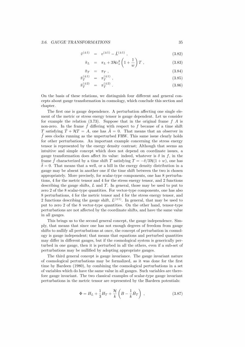
On the basis of these relations, we distinguish four different and general con-cepts about gauge transformation in cosmology, which conclude this section andchapter.
The first one is gauge dependence. A perturbation affecting one single ele-ment of the metric or stress energy tensor is gauge dependent. Let us considerfor example the relation (3.73). Suppose that in the original frame f A isnon-zero. In the frame f differing with respect to f because of a time shiftT satisfying T + HT = A, one has A = 0. That means that an observer inf sees clocks running as the unperturbed FRW. This same issue clearly holdsfor other perturbations. An important example concerning the stress energytensor is represented by the energy density contrast; Although that seems anintuitive and simple concept which does not depend on coordinate issues, agauge transformation does affect its value: indeed, whatever is δ in f , in theframe f characterized by a time shift T satisfying T = −δ/3H(1 + w), one hasδ = 0. That means that a well, or a hill in the energy density distribution in agauge may be absent in another one if the time shift between the two is chosenappropriately. More precisely, for scalar-type components, one has 8 perturba-tions, 4 for the metric tensor and 4 for the stress energy tensor, and 2 functionsdescribing the gauge shifts, L and T . In general, those may be used to put tozero 2 of the 8 scalar-type quantities. For vector-type components, one has also8 perturbations, 4 for the metric tensor and 4 for the stress energy tensor, and2 functions describing the gauge shift, L(±1). In general, that may be used toput to zero 2 of the 8 vector-type quantities. On the other hand, tensor-typeperturbations are not affected by the coordinate shifts, and have the same valuein all gauges.
This brings us to the second general concept, the gauge independence. Sim-ply, that means that since one has not enough degrees of freedom from gaugeshifts to nullify all perturbations at once, the concept of perturbation in cosmol-ogy is gauge independent; that means that equations and perturbed quantitiesmay differ in different gauges, but if the cosmological system is generically per-turbed in one gauge, then it is perturbed in all the others, even if a sub-set ofperturbations may be nullified by adopting appropriate gauges.
The third general concept is gauge invariance. The gauge invariant natureof cosmological perturbations may be formalized, as it was done for the firsttime by Bardeen (1980), by combining the cosmological perturbations in a setof variables which do have the same value in all gauges. Such variables are there-fore gauge invariant. The two classical examples of scalar-type gauge invariantperturbations in the metric tensor are represented by the Bardeen potentials:
Φ = HL +1
3HT +
Hk
(B − 1
kHT
), (3.87)
36CHAPTER 3. CLASSIFICATION OF LINEAR COSMOLOGICAL PERTURBATIONS
Ψ = A+Hk
(B − 1
kHT
)+
1
k
(B − 1
kHT
). (3.88)
By exploiting the relations (3.73,3.74,3.76,3.76), it is easy to verify that Φ = Φ,Ψ = Ψ. Any linear combination of them involving factors made by constantsor background quantities is gauge invariant as well. On the other hand, forvector-type perturbations, the gauge invariant metric perturbation is unique:
σ(±1)g = B(±1) − 1
kH
(±1)T . (3.89)
Note that also the scalar-type version of (3.89), B − HT /k is gauge invariant.Two conventient choices of gauge invariant quantities involving quantities re-lated to the stress energy tensor are
∆ = δ +3H(1 + w)
k(v −B) , (3.90)
V = v − 1
kHT , (3.91)
which generalize density contrast and peculiar velocity, respectively. As for themetric tensor, such choice is not unique as any combination of the quantitiesabove is gauge invariant as well. It is interesting to build up two gauge invariantquantities involving the stress energy tensor only:
Γ = πL −c2swδ , (3.92)
πT . (3.93)
Γ has a direct physical meaning in terms of thermal equilibrium of the compo-nents in the cosmic fluid. Indeed, the condition Γ = 0 implies
πL ≡δp
p=c2swδ ≡ c2s
w
δρ
ρ, (3.94)
which is equivalent toδp
δρ=p
ρ. (3.95)
The condition above is known as adiabaticity. As we see now, the reason is thatit is satisfied when a given cosmological system characterized by thermal equi-librium possesses perturbations which do not break it. Let’s suppose to have aradiation component at thermal equilibrium, characterized by p = wρ = ρ/3.Γ is zero when also δp = δρ/3, which means that pressure fluctuations followadiabatically those of the energy density, keeping thermal equilibrium for radi-ation, specified by the condition w = 1/3, valid everywhere. Note that this isnot true in general: δp = (δw)ρ+ w(δρ). That is, if w fluctuates, then thermalequilibrium is also perturbed, and this is expressed by the fact that the adia-baticity condition (3.95) is violated.Finally, let us define two relevant vector-type stress energy tensor gauge invari-ant quantities, which are merely a generalization of (3.91) and (3.93):
V (±1) = v(±1) − 1
kH
(±1)T , (3.96)
3.6. GAUGE TRANSFORMATIONS 37
π(±1)T . (3.97)
Again the tensor-type stress energy tensor perturbation, π(±2)T , is gauge invari-
ant as no gauge coordinate shift is tensor-type.We now come to the last point, the gauge spuriosity. In extreme synthe-
sis, the issue is that different observers, belonging to different gauges, may seethe same numerical value of cosmological perturbations; the coordinate shiftsamong those observers are not to be confused with cosmological perturbations,representing spurious gauge modes. The best way to see this point is to considertwo most popular example of gauges.The synchronous gauge is defined by using T , L and L(±1) in such a way toconfine the perturbations in the metric tensor to the spatial area only:
A = B = B(±1) = 0 . (3.98)
As we have already seen, the first condition above means that the time shiftbetween f and f must satisfy the condition
T +HT = A . (3.99)
The solution to this equation is not unique. Actually, there are infinite solutions,made by the sum of a particular one, plus all the solutions of the homogeneousequation, T +HT = 0, which is satisfied by Tg ∝ 1/a. This means that thereare an infinite number of frames which are in the synchronous gauge. The gaugemode Tg is spurious in the sense that it is not a cosmological perturbation, butjust the time shift between all frames seeing the same value of A. Spuriousgauge modes usually affect several quantities: for example, the energy densityfluctuation picks up a spurious gauge mode given by
δg = 3H(1 + w)Tg . (3.100)
Moreover, the second condition in (3.98), which is written as
L+ kT = −B , (3.101)
does not determine L uniquely; indeed, all frames differing by a shift given by
Lg = −k∫Tgdτ + constant (3.102)
are in the synchronous gauge. This also produces a gauge spurious mode in thevelocity:
vg = −Lg . (3.103)
Finally, also the third condition in (3.98) leaves a constant spurious vector-type
gauge mode, L(±1)g = constant. In principle, one may track the spurious gauge
modes in the computations, or adopt a specific synchronous gauge by fixing allconstants. In practice however, it is much better to perform those in a gaugewithout spuriosity. We see now an example of gauge where that is absent.The Newtonian gauge is specified by
B = HT = H(±1)T = 0 , (3.104)
38CHAPTER 3. CLASSIFICATION OF LINEAR COSMOLOGICAL PERTURBATIONS
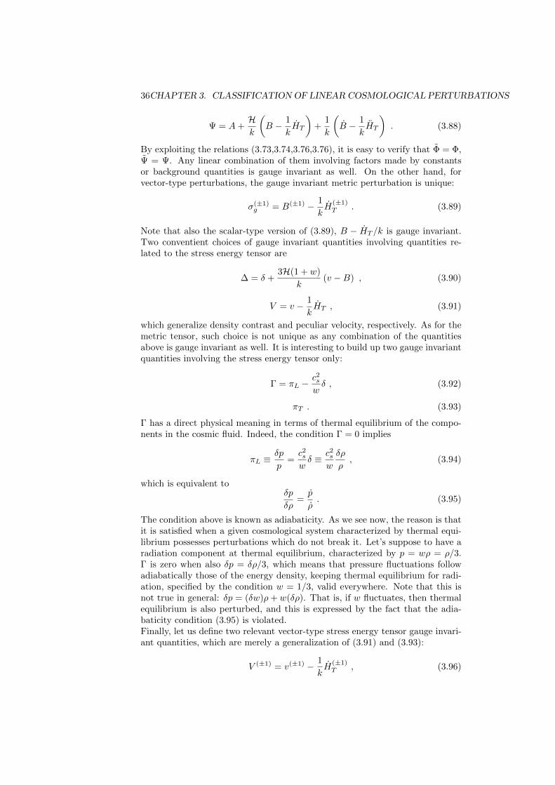
Figure 3.5: The behavior of physical distances versus the one of the effectivehorizon in the MDE and RDE.
thus allowing the perturbed metric tensor to be non-null on the diagonal onlyin the scalar-type component. It is easy to see that the second condition issatisfied performing a coordinate change between f and f such that
L = −1
kHT , (3.105)
which is uniquely fixed. The second condition also fixes uniquely T :
T = −1
k
(B + L
). (3.106)
Similarly, at the vector-type level the coordinate transformation needed to goin the Newtonian gauge is
L(±1) = −1
kH
(±1)T , (3.107)
which completes the set of coordinate shifts necessary to go in the Newtoniangauge. This is therefore an example where gauge spuriosity is absent. In con-clusion, spurious gauge modes may activate or even accidentally put to zerocosmological perturbation modes in energy density, velocity, or metric fluctua-tions. By working in a gauge free of spuriosity, one is sure that all the solutionsof the cosmological perturbation evolution equations are physical, unaffected bygauge modes.
3.7 excercises
3.7.1 question about the cosmological perturbations alge-bra and metric tensor fluctuations
Consider the perturbed metric in cosmology with the two combinations of in-deces:
gµν = gµν + δgµν , gµν = gµν + δgµν . (3.108)
3.7. EXCERCISES 39
By exploiting the usual relation gµ′ν′ = gµ
′µgν′ν gµν in the linear approximation,
find the general relation between δgµν and δgµν . By knowing that in the Fourierspace the scalar-type components of the spatial metric perturbation are
δg00 = a2h00 = −2a2AY , δg0i = a2h0i = −a2BYi ,
δgij = a2hij = 2a2(HLY γij +HTYij) , (3.109)
find the expression of the Fourier amplitude for δg00, δg0i, δgij . Assume spatialflatness, K = 0, so that the background metric tensor may be expressed asgµν = a2ηµν , gµν = a−2ηµν where ηµν is the Minkowski metric.
3.7.2 question about the cosmological perturbations alge-bra and stress energy tensor fluctuations
Consider the perturbed metric and stress energy tensors in cosmology:
gµν = gµν + δgµν , T νµ = T νµ + δT νµ , (3.110)
where gµν = a2γµν and T νµ are the background metric and stress energy tensor,respectively. By exploiting the rules for rising indeces in general relativity, onehas δgµν = −gµµ′gνν′δgµ′ν′ . Find the corresponding relation for δTµν as afunction of δT νµ . Considering scalar-type perturbations only, and defining theFourier space amplitudes
δg00 = −2a2AY , δT ji = p(πLY δji + πTY
ji ) , (3.111)
find the expression of δg00, δT ij , using the fact that the indeces for Yij areraised and lowered with the spatial metric γij .
3.7.3 question about gauge invariant formalism
By exploiting the gauge transformation laws, demonstrate that the metric fluc-tuation quantities
A = A− 1
a
d
dτ
[(a2
a
)(HL +
1
3HT
)],
B = B +k
H
(HL +
1
3HT
)− 1
kHT (3.112)
are gauge invariant.

40CHAPTER 3. CLASSIFICATION OF LINEAR COSMOLOGICAL PERTURBATIONS

Chapter 4
Linear cosmologicalperturbation dynamics
41
42CHAPTER 4. LINEAR COSMOLOGICAL PERTURBATION DYNAMICS
4.1 analysis of the perturbed einstein and con-servation equations
In this section we write the evolution equations for cosmological perturbations,and we perform a phenomenological study of their solutions. Most of that isreflected in the properties of CMB anisotropies, as we shall see in the followingchapters.
4.1.1 effective horizon
The first thing to do when studying the dynamics of cosmological perturbationson a given scale λ is to compare it with a suitable definition of the horizon,i.e. a physical length expressing the maximum scale reached by physical inter-actions at a given time. On scales larger than the horizon, which are namedsuper-horizon, no dynamics is allowed from those physical interactions. On sub-horizon scales, the dynamics is active. In general relativity the causal horizonis the distance traveled by photons in a given time interval t1, t2 for a givenobserver. In a FRW metric, by posing ds2 = 0 one sees immediately that
causal horizon =
∫ t2
t1
dt
a= τ2 − τ1 , (4.1)
where τ as usual represents the conformal time. On the other hand, this turnsout not to be a suitable definition of cosmological horizon, since it does nottake into account the specific interactions present into the system, other thanlight propagation. For this reason, in cosmology an effective horizon is defined,different from the causal one, but suitably affecting all the relevant dynamics ofcosmological perturbations: that is simply the inverse of the Hubble expansionrate:
effective horizon = H−1 = aH−1 . (4.2)
In the following, we will refer to the quantity above as effective horizon, Hubblehorizon, or simply horizon, giving an order of magnitude estimate of the distancewithin physical interactions can occur. Despite of the fact that acting effectivelyas a causal horizon is a most important property, there is no rigorous demon-stration showing that H−1 possesses it. Empirically, however, that is the alwaysthe case: in any problem in cosmology concerning the dynamics of cosmologicalperturbations, H−1 separates the sub-horizon and super-horizon regimes, i.e.scales where the physical interactions can or cannot occur, respectively. Anhint that this is the case may be seen from the background conservation equa-tion, ρ + 3H(ρ + p). H−1 sets the physical time scale for the fluid dynamics.On time scales much smaller, ρ is frozen; on much larger scales, ρ may varysignificantly. The same happens for distances when looking at the perturbationequations.
4.1.2 sub-horizon and super-horizon scales
The dynamics of cosmological perturbations is markedly different if a givenscale at a give time is smaller or larger than the horizon. For this reason,the dynamical description is given separately for the sub-horizon and super-horizon regimes, meaning for scales which are smaller or larger than the horizon,
4.1. ANALYSIS OF THE PERTURBED EINSTEIN AND CONSERVATION EQUATIONS43
respectively. In this respect, the first thing to do is studying the time dependenceof horizon and a given physical scale, in order to determine the sequences of sub-horizon and super-horizon epochs. It is convenient to compare the dependenceof the effective horizon and scales on a rather than on time. While physicalscales λp depend linearly on it, from the Friedmann equation in a flat FRW it iseasy to see that in cosmologies where a ∝ tp, the Hubble horizon is H−1 ∝ a1/p.Therefore, in the RDE and MDE, the behavior of λp versusH−1 may be sketchedas
RDE :λp = λa , H−1 = H−10 a3/2
eq a2 ,
MDE :λp = λa , H−1 = H−10 a3/2 , (4.3)
where λ and H−10 are evaluated at a given time, corresponding for example to
the present where we set a = 1, and the combination H−10 a
3/2eq gives the value
of H−1 at equivalence approximating the passage between MDE and RDE asinstantaneous. As shown in figure 3.5, in the MDE and RDE the growth of H−1
is always stronger than the one of λp. That means that in this cosmologicalscenario, for each physical distance there is only one time when that is equal tothe horizon. This means that regions separated by that scale can never interactwith each other before that time. On the other hand, after that they are alwayswithin the horizon and mutual interactions are allowed.
4.1.3 equations for scalar-type perturbations
We exploit tge gauge invariant language in terms of ∆, V , Γ, πT defined previ-ously. The Einstein equations give(
k2
a2−K
)Φ = 4πGρ∆ , (4.4)
k2
a2(Φ + Ψ) = −8πGpπT . (4.5)
The first equation is analogous to the Poisson one in the Newtonian theory ofgravity. The second equation is purely general relativistic, determining the ex-istence of two independent scalar gravitational potentials. Note that in absenceof anisotropic stress, the scalar-type fluctuations become essentially Newtonian,as Φ = −Ψ, and the only relevant equation is the Poisson one.The conservation of the stress energy tensor gives the general relativistic ex-pression for the continuity and Euler equations, respectively:
∆− 3wH∆ =
(3K
k2− 1
)(1 + w) kV + 2
(3K
k2− 1
)HwπT , (4.6)
V +HV = k
(4πGa2ρ
k2 − 3K− c2s
1 + w
)∆ + k
w
1 + wΓ−
−[
8πGa2ρ
k2+
(1
3− K
k2
)]kwπT . (4.7)
Notice the friction caused by the cosmological expansion in the Euler equation,second term in the left hand side. The anti-friction in the left hand side ofthe continuity equation is only apparent, as the combination with the term
44CHAPTER 4. LINEAR COSMOLOGICAL PERTURBATION DYNAMICS
containinig V in general yields a friction term again, as we see in the followingin some relevant examples. The continuity equation may be derived once in theconformal time. The consequent term in V may be expressed in terms of V , ∆,Γ and πT using the Euler equation. Moreover, the terms proportional to V maybe expressed in terms of ∆, ∆, πT using the continuity equation again. Theresult is a second order equation in ∆, which will be useful in the following. Itsexpression is
∆−[3(2w − c2s
)− 1]H∆+
+
[(3
2w2 − 4w + 3c2s −
1
2
)H2 +
3w2 − 1
2K +
k2 − 3K
3c2s
]3∆ = S , (4.8)
where the source term is represented by
S = −(k2 − 3K)wΓ− 2
(1− 3K
k2
)HwπT +
(1− 3K
k2
)2πT ·
·[
3(w2 + c2s
)− 2w
]H2 + w (3w + 2)K +
k2 −K3
c2s
. (4.9)
Despite of its cumbersome look, this is the equation that we shall exploit for aphenomenological analysis of the dynamics of cosmological perturbations. Notethat the four independent equations above account for the evolution of fourcorresponding unknowns, the two gravitational potentials and only two of thefour variables concerning the fluid. Independent conditions, usually relatedto the nature of the fluid, are needed in order to specify the extra-degrees offreedom. of the system. In practical applications, this means specifying howthe isotropic and anisotropic pressure perturbations represented by Γ and πTare linked to the other variables, e.g. density ∆ and velocity V , in analogy towhat is done for the background, where the pressure p is expressed in terms ofρ.
4.1.4 equations for vector-type perturbations
We exploit the three gauge invariant quantities σ(±1)g , V (±1) and π
(±1)T , account-
ing for metric and stress energy tensor perturbations associated to vorticity. TheEinstein equations give
8πG(ρ+ p)V (±1) =2K − k2
2a2σ(±1)g , (4.10)
σ(±1)g + 2Hσ(±1)
g = 8πGa2
k2pπ
(±1)T , (4.11)
which may be combined into
V (±1) + (1− 3c2s)HV (±1) =2K − k2
2k
w
1 + wπ
(±1)T . (4.12)
Notice that again, one degree of freedom, for example the anisotropic pressureperturbation represented by πT , has to be expressed in terms of the others inorder to achieve a solution of the system.
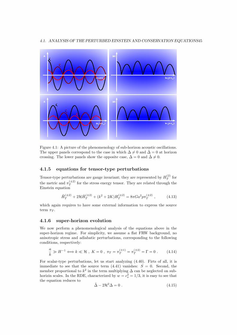
4.1. ANALYSIS OF THE PERTURBED EINSTEIN AND CONSERVATION EQUATIONS45
Figure 4.1: A picture of the phenomenology of sub-horizon acoustic oscillations.The upper panels correspond to the case in which ∆ 6= 0 and ∆ = 0 at horizoncrossing. The lower panels show the opposite case, ∆ = 0 and ∆ 6= 0.
4.1.5 equations for tensor-type perturbations
Tensor-type perturbations are gauge invariant; they are represented by H(2)T for
the metric and π(±2)T for the stress energy tensor. They are related through the
Einstein equation
H(±2)T + 2HH(±2)
T + (k2 + 2K)H(±2)T = 8πGa2pπ
(±2)T , (4.13)
which again requires to have some external information to express the sourceterm πT .
4.1.6 super-horizon evolution
We now perform a phenomenological analysis of the equations above in thesuper-horizon regime. For simplicity, we assume a flat FRW background, noanisotropic stress and adiabatic perturbations, corresponding to the followingconditions, respectively:
a
k H−1 ⇐⇒ k H , K = 0 , πT = π
(±1)T = π
(±2)T = Γ = 0 . (4.14)
For scalar-type perturbations, let us start analyzing (4.40). Firts of all, it isimmediate to see that the source term (4.41) vanishes: S = 0. Second, themember proportional to k2 in the term multiplying ∆ can be neglected on sub-horizin scales. In the RDE, characterized by w = c2s = 1/3, it is easy to see thatthe equation reduces to
∆− 2H2∆ = 0 . (4.15)
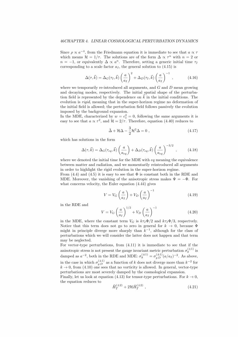
46CHAPTER 4. LINEAR COSMOLOGICAL PERTURBATION DYNAMICS
Since ρ ∝ a−4, from the Friedmann equation it is immediate to see that a ∝ τwhich means H = 1/τ . The solutions are of the form ∆ ∝ τn with n = 2 orn = −1, or equivalently ∆ ∝ an. Therefore, setting a generic initial time τIcorresponding to a scale factor aI , the general solution to (4.15) is
∆(τ,~k) = ∆G(τI ,~k)
(a
aI
)2
+ ∆D(τI ,~k)
(a
aI
)−1
, (4.16)
where we temporarily re-introduced all arguments, and G and D mean growingand decaying modes, respectively. The initial spatial shape of the perturba-tion field is represented by the dependence on ~k in the initial conditions. Theevolution is rigid, meaning that in the super-horizon regime no deformation ofthe initial field is allowed; the perturbation field follows passively the evolutionimposed by the background expansion.In the MDE, characterized by w = c2s = 0, following the same arguments it iseasy to see that a ∝ τ2, and H = 2/τ . Therefore, equation (4.40) reduces to
∆ +H∆− 3
2H2∆ = 0 , (4.17)
which has solutions in the form
∆(τ,~k) = ∆G(τeq,~k)
(a
aeq
)+ ∆D(τeq,~k)
(a
aeq
)−3/2
, (4.18)
where we denoted the initial time for the MDE with eq meaning the equivalencebetween matter and radiation, and we momentarily reintroduced all argumentsin order to highlight the rigid evolution in the super-horizon regime.From (4.4) and (4.5) it is easy to see that Φ is constant both in the RDE andMDE. Moreover, the vanishing of the anisotropic stress makes Ψ = −Φ. Forwhat concerns velocity, the Euler equation (4.44) gives
V = VG
(a
aI
)+ VD
(a
aI
)−1
(4.19)
in the RDE and
V = VG
(a
aI
)1/2
+ VD
(a
aI
)−1
(4.20)
in the MDE, where the constant term VG is kτIΦ/2 and kτIΦ/3, respectvely.Notice that this term does not go to zero in general for k → 0, because Φmight in principle diverge more sharply than k−1, although for the class ofperturbations which we will consider the latter does not happen and that termmay be neglected.For vector-type perturbations, from (4.11) it is immediate to see that if the
anisotropic stress is not present the gauge invariant metric perturbation σ(±1)g is
damped as a−2, both in the RDE and MDE: σ(±1)g = σ
(±1)g D (a/aI)
−2. As above,
in the case in which σ(±1)g D as a function of k does not diverge more than k−2 for
k → 0, from (4.10) one sees that no vorticity is allowed. In general, vector-typeperturbations are most severely damped by the cosmological expansion.Finally, let us look at equation (4.13) for tensor-type perturbations. For k → 0,the equation reduces to
H(±2)T + 2HH(±2)
T , (4.21)

4.1. ANALYSIS OF THE PERTURBED EINSTEIN AND CONSERVATION EQUATIONS47
Figure 4.2: A picture of the phenomenology of sub-horizon dynamics in thecase in which both ∆ and ∆ are active at horizon crossing, destroying the phasecoherence.
which has solutions both in the RDE and MDE in the form
H(±2)T = H
(±2)T C +H
(±2)T D
(a
aI
)−2
. (4.22)
The above equation means that on super-horizon scales, cosmological gravita-tional waves admit a constant solution, a most important feature in order to beable to detect them in modern experiments.
4.1.7 sub-horizon evolution
We now discuss the phenomenology occurring on sub-horizon scales. The re-maining hypotheses are unchanged with respect to (4.14):
K = 0 , πT = π(±1)T = π
(±2)T = Γ = 0 . (4.23)
In the RDE the equation of state is c2s = 1/3, so that in the limit of infintehorizon, or H → 0, in the left hand side of equation (4.40) the first and the lastterms are the only ones which survive, while the source term (4.41) vanishesagain. The left hand side of (4.40) simplifies drastically:
∆ + k2c2s∆ = 0 . (4.24)
The general solution is
∆(τ,~k) = ∆0(τHC ,~k) cos[kcs(τ −τHC)]+∆1(τHC ,~k) sin[kcs(τ −τHC)] , (4.25)
where we have momentarily reintroduced all arguments, and by HC we meanthe horizon crossing, i.e. roughly the initial time from which we can considerthat the solution is well represented by (4.25). It is immediate to see that thereare two distinct types of initial conditions. If ∆0 6= 0 at τHC , ∆ 6= 0 as well,with zero velocity and peaks in kcs(τ − τHC) = nπ and zeros at kcs(τ − τHC) =(n + 1/2)π, for integer n. If ∆1 6= 0 at τHC , ∆ = 0 while ∆ 6= 0, with peaksin kcs(τ − τHC) = (n + 1/2)π and zeros at kcs(τ − τHC) = nπ, for integern. It is important to point out that, if the solution is characterized by either∆0 6= 0, ∆1 = 0 or ∆0 = 0, ∆1 6= 0 at τHC all Fourier modes ~k such that |~k| = khave peaks and zeros in the same locations, and so their superposition, although
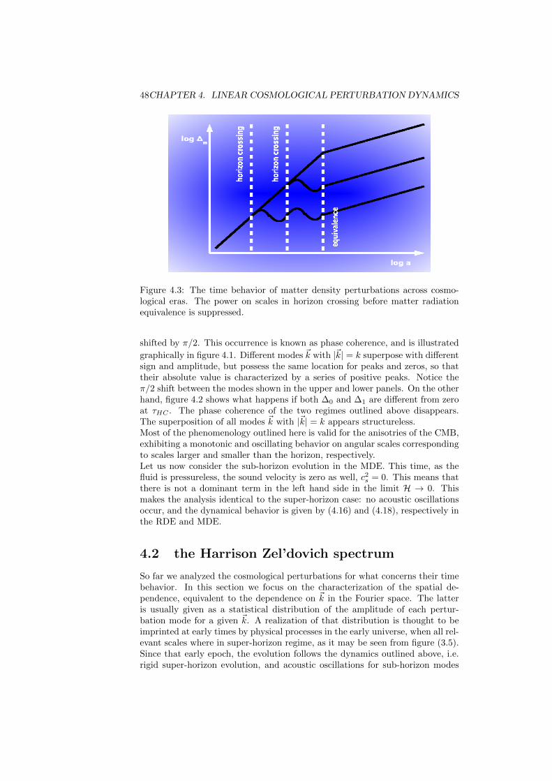
48CHAPTER 4. LINEAR COSMOLOGICAL PERTURBATION DYNAMICS
Figure 4.3: The time behavior of matter density perturbations across cosmo-logical eras. The power on scales in horizon crossing before matter radiationequivalence is suppressed.
shifted by π/2. This occurrence is known as phase coherence, and is illustrated
graphically in figure 4.1. Different modes ~k with |~k| = k superpose with differentsign and amplitude, but possess the same location for peaks and zeros, so thattheir absolute value is characterized by a series of positive peaks. Notice theπ/2 shift between the modes shown in the upper and lower panels. On the otherhand, figure 4.2 shows what happens if both ∆0 and ∆1 are different from zeroat τHC . The phase coherence of the two regimes outlined above disappears.The superposition of all modes ~k with |~k| = k appears structureless.Most of the phenomenology outlined here is valid for the anisotries of the CMB,exhibiting a monotonic and oscillating behavior on angular scales correspondingto scales larger and smaller than the horizon, respectively.Let us now consider the sub-horizon evolution in the MDE. This time, as thefluid is pressureless, the sound velocity is zero as well, c2s = 0. This means thatthere is not a dominant term in the left hand side in the limit H → 0. Thismakes the analysis identical to the super-horizon case: no acoustic oscillationsoccur, and the dynamical behavior is given by (4.16) and (4.18), respectively inthe RDE and MDE.
4.2 the Harrison Zel’dovich spectrum
So far we analyzed the cosmological perturbations for what concerns their timebehavior. In this section we focus on the characterization of the spatial de-pendence, equivalent to the dependence on ~k in the Fourier space. The latteris usually given as a statistical distribution of the amplitude of each pertur-bation mode for a given ~k. A realization of that distribution is thought to beimprinted at early times by physical processes in the early universe, when all rel-evant scales where in super-horizon regime, as it may be seen from figure (3.5).Since that early epoch, the evolution follows the dynamics outlined above, i.e.rigid super-horizon evolution, and acoustic oscillations for sub-horizon modes
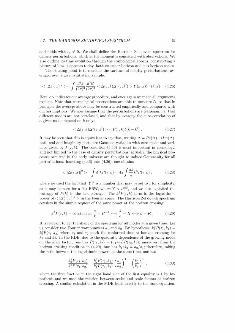
4.2. THE HARRISON ZEL’DOVICH SPECTRUM 49
and fluids with cs 6= 0. We shall define the Harrizon Zel’dovich spectrum fordensity perturbations, which at the moment is consistent with observations. Wealso outline its time evolution through the cosmological epochs, constructing apicture of how it appears today, both on super-horizon and sub-horizon scales.
The starting point is to consider the variance of density perturbations, av-eraged over a given statistical sample:
< |∆(τ, ~x)|2 >=
∫d3k
(2π)3
d3k′
(2π)3< ∆(τ,~k)∆∗(τ,~k′) > Y (~k, ~x)Y ∗(~k, ~x) . (4.26)
Here <> indicates our average procedure, and once again we made all argumentsexplicit. Note that cosmological observations are able to measure ∆, so that inprinciple the average above may be constructed empirically and compared withour assumptions. We now assume that the perturbations are Gaussian, i.e. thatdifferent modes are not correlated, and that by isotropy the auto-correlation ofa given mode depend on k only:
< ∆(τ,~k)∆∗(τ,~k′) >= P (τ, k)δ(~k − ~k′) . (4.27)
It may be seen that this is equivalent to say that, writing ∆ = Re(∆)+ iIm(∆),both real and imaginary parts are Gaussian variables with zero mean and vari-ance given by P (τ, k). The condition (4.46) is most important in cosmology,and not limited to the case of density perturbations; actually, the physical pro-cesses occurred in the early universe are thought to induce Gaussianity for allperturbations. Inserting (4.46) into (4.26), one obtains
< |∆(τ, ~x)|2 >=
∫d3kP (τ, k) = 4π
∫dk
kk3P (τ, k) , (4.28)
where we used the fact that |Y |2 is a number that may be set to 1 for simplicity,
as it may be seen for a flat FRW, where Y ∝ ei~k~x, and we also exploited the
isotropy of P (k) in the last passage. The k3P (τ, k) term is the logarithmicpower of < |∆(τ, ~x)|2 > in the Fourier space. The Harrison Zel’dovich spectrumconsists in the simple request of the same power at the horizon crossing:
k3P (τ, k) = constant ata
k= H−1 ⇐⇒ k
a= H ⇐⇒ k = H . (4.29)
It is relevant to get the shape of the spectrum for all modes at a given time. Letus consider two Fourier wavenumvers k1 and k2. By hypothesis, k3
1P (τ1, k1) =k3
2P (τ1, k2) where τ1 and τ2 mark the conformal time at horizon crossing fork1 and k2. In the RDE, due to the quadratic dependence of the growing modeon the scale factor, one has P (τ1, k2) = (a1/a2)P (τ2, k2); moreover, from thehorizon crossing condition in (4.29), one has k1/k2 = a2/a1; therefore, takingthe ratio between the logarithmic powers at the same time, one has
k32P (τ1, k2)
k31P (τ1, k2)
=k3
2P (τ2, k2)
k31P (τ1, k2)
(a1
a2
)4
=
(k2
k1
)4
, (4.30)
where the first fraction in the right hand side of the first equality is 1 by hy-pothesis and we used the relation between scales and scale factors at horizoncrossing. A similar calculation in the MDE leads exactly to the same equation,

50CHAPTER 4. LINEAR COSMOLOGICAL PERTURBATION DYNAMICS
Figure 4.4: A picture of the matter power spectrum today. The suppression ofpower on scales smaller than the horizon at equivalence creates a characteristicpeak at the comoving wavenumber corresponding to the Horizon at equivalencein comoving coordinates, keq.
minding that perturbations now grow as a and modifying suitably the relationbetween scales and scale factors at the horizon crossing. Since the choice of ksis purely conventionally, we conclude that the Harrison Zel’dovich spectrum asseen at a given time as a function of k is
P (τ, k) ∝ k . (4.31)
The spectrum is known as scale invariant, because of the property of yieldingthe same Fourier logarithmic power in < |∆(τ,~k)| > at the horizon crossing.Deviations from scale invariance are parametrized through the introduction ofthe scalar spectral index for perturbations, ns, such that
P (τ, k) ∝ kns , (4.32)
where ns = 1 reduces to the pure scale invariance.
4.3 the power spectrum of matter perturbationstoday
As it was seen in the previous sections, all relevant scales in cosmology, saybetween 1 and a few thousands Mpc, were on super-horizon regime at the initialtime in the RDE. Therefore (4.32) describe statistically the initial conditionof cosmological density fluctuations. We now outline the phenomenology ofthe time evolution of P (k) through the cosmological epochs, using the resultsobtained in the previous sections. In particular, we describe the appearence of(4.32) at present.First, let us extend our formalism to represent a two component system, madeby relativistic (r) and non-relativistic matter (m); the treatment developed inthis chapter may be easily extended to a multi-component system (Kodama &
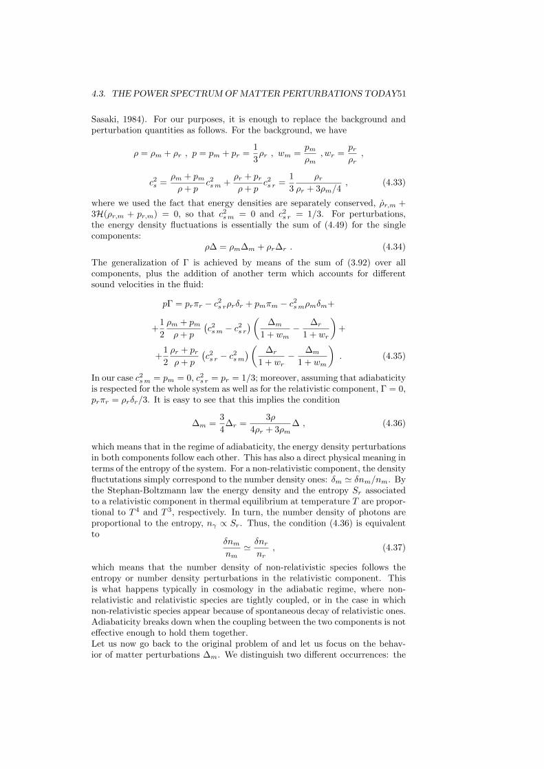
4.3. THE POWER SPECTRUMOFMATTER PERTURBATIONS TODAY51
Sasaki, 1984). For our purposes, it is enough to replace the background andperturbation quantities as follows. For the background, we have
ρ = ρm + ρr , p = pm + pr =1
3ρr , wm =
pmρm
, wr =prρr
,
c2s =ρm + pmρ+ p
c2sm +ρr + prρ+ p
c2s r =1
3
ρrρr + 3ρm/4
, (4.33)
where we used the fact that energy densities are separately conserved, ρr,m +3H(ρr,m + pr,m) = 0, so that c2sm = 0 and c2s r = 1/3. For perturbations,the energy density fluctuations is essentially the sum of (4.49) for the singlecomponents:
ρ∆ = ρm∆m + ρr∆r . (4.34)
The generalization of Γ is achieved by means of the sum of (3.92) over allcomponents, plus the addition of another term which accounts for differentsound velocities in the fluid:
pΓ = prπr − c2s rρrδr + pmπm − c2smρmδm+
+1
2
ρm + pmρ+ p
(c2sm − c2s r
)( ∆m
1 + wm− ∆r
1 + wr
)+
+1
2
ρr + prρ+ p
(c2s r − c2sm
)( ∆r
1 + wr− ∆m
1 + wm
). (4.35)
In our case c2sm = pm = 0, c2s r = pr = 1/3; moreover, assuming that adiabaticityis respected for the whole system as well as for the relativistic component, Γ = 0,prπr = ρrδr/3. It is easy to see that this implies the condition
∆m =3
4∆r =
3ρ
4ρr + 3ρm∆ , (4.36)
which means that in the regime of adiabaticity, the energy density perturbationsin both components follow each other. This has also a direct physical meaning interms of the entropy of the system. For a non-relativistic component, the densityfluctutations simply correspond to the number density ones: δm ' δnm/nm. Bythe Stephan-Boltzmann law the energy density and the entropy Sr associatedto a relativistic component in thermal equilibrium at temperature T are propor-tional to T 4 and T 3, respectively. In turn, the number density of photons areproportional to the entropy, nγ ∝ Sr. Thus, the condition (4.36) is equivalentto
δnmnm' δnr
nr, (4.37)
which means that the number density of non-relativistic species follows theentropy or number density perturbations in the relativistic component. Thisis what happens typically in cosmology in the adiabatic regime, where non-relativistic and relativistic species are tightly coupled, or in the case in whichnon-relativistic species appear because of spontaneous decay of relativistic ones.Adiabaticity breaks down when the coupling between the two components is noteffective enough to hold them together.Let us now go back to the original problem of and let us focus on the behav-ior of matter perturbations ∆m. We distinguish two different occurrences: the
52CHAPTER 4. LINEAR COSMOLOGICAL PERTURBATION DYNAMICS
perturbations gets in horizon crossing before matter radiation equality, or after.In the super-horizon regime, by virtue of (4.36) ∆m grows as a2 before matterradiation equality and as ∆ ∝ a later. In the sub-horizon regime, ∆m osclil-lates before matter radiation equality, because by adiabaticity it’s dragged bythe acoustic oscillations in ∆r; but later, in the MDE, it starts to grow againas a, because the sound velocity (4.33) vanishes in the MDE. Summarizing,∆m always grows if the horizon crossing occurs later than the matter radiationequality. Viceversa, it stays constant between the horizon crossing and matterradiation equality. This means that on wavenumbers corresponding to scaleswhich had the horizon crossing before matter radiation equality, the power issuppressed with respect to the others. The smaller the scale, the larger is thetime interval between horizon crossing and matter radiation equality, the largeris the suppression. Therefore, at present, scales larger than the horizon at equiv-alence still exhibit the primordial power represented by (4.2) for an HarrisonZel’dovich spectrum; scales smaller than that are suppressed. The time behav-ior of ∆m on different scales is shown in figure (4.3), for simplicity assuming thesame power at the beginning for all scales. The appearence of the matter powerspectrum today is shown in figure (4.4), assuming an initial Harrizon Zel’dovichspectrum. The primordial power, proportional to k, is visible at wavenumberscorresponding to scales larger than the one which crosses the horizon at equiva-lence. On larger wavelengths, the suppression occurs because of the mechanismoutlined above.
4.4 excercises
4.4.1 question about effective horizon and cosmologicalscales
The behavior of the Hubble effective horizon as a function of the scale factor isapproximately
H−1 ∝ a3/2 in the matter dominated era, (4.38)
H−1 ∝ a2 in the radiation dominatedera. (4.39)
Its value today is H−10 ' 10000 Mpc. The matter energy density today is
ρc ' 10−29 g/cm3, while the radiation one is about 105 times smaller. Find theproportionality constants in (4.38,4.39) assuming continuity at the equivalencebetween matter and radiation; for simplicity, you may set to unity the value ofthe scale factor today, a0 = 1.By assuming that the radiation dominated era begins when its energy densitycorresponds to the Planck energy scale, ρP ' 10123 · ρc, calculate the value ofthe scale factor at that epoch, aR.By assuming that at earlier times the universe was inflationary, i.e. constant H,calculate the ratio aR/aHC , where aHC is the value of the scale factor when thecosmological scale corresponding to the effective horizon today was in horizoncrossing during inflation.
4.4. EXCERCISES 53
4.4.2 question about density perturbations in a cosmolog-ical constant dominated cosmology
Consider the second order evolution equation for the gauge invariant densitycontrast ∆:
∆−[3(2w − c2s
)− 1]H∆+
+
[(3
2w2 − 4w + 3c2s −
1
2
)H2 +
3w2 − 1
2K +
k2 − 3K
3c2s
]3∆ = S , (4.40)
where the source term is represented by
S = −(k2 − 3K)wΓ− 2
(1− 3K
k2
)HwπT +
(1− 3K
k2
)2πT ·
·[
3(w2 + c2s
)− 2w
]H2 + w (3w + 2)K +
k2 −K3
c2s
. (4.41)
Assume no anisotropic stress, spatial flatness, adiabaticity, super-horizon scales,k → 0. Also assume that the cosmological expansion is dominated by a cosmo-logical constant Λ, yielding a constant Hubble expansion rate given by
H2 =Λ
3= constant , (4.42)
and mimicking a fluid with w = c2s = −11. Solve equation (4.40) in thesehypotheses, and show that ∆ is exponentially damped as a function of theordinary time t.
4.4.3 question about the super-horizon scalar-type pecu-liar velocity
Consider the Fourier space amplitudes ∆ and V of the scalar-type gauge invari-ant density contrast and peculiar velocity. Their evolution equation, derivedfrom δ(T νi;ν) = 0, in a flat Friedmann Robertson Walker (FRW) metric withadiabatic perturbations and no anisotropic stress, are
∆− 3wH∆ = − (1 + w) kV , (4.43)
V +HV = kΦ− c2s1 + w
∆ . (4.44)
where Φ is the generalized Bardeen potential. Determine the solutions for V onsuper-horizon scales, in the matter and radiation dominated eras.
4.4.4 question about the Harrison Zel’dovich power spec-trum for gravitational waves
Consider tensor-type perturbations in the FRW metric:
h(±2)ij (τ, ~x) = 2
∫d3k
(2π)3H
(±2)T (τ,~k)Y
(±2)ij (~x,~k) . (4.45)
1Notice that the sound velocity, c2s = p/ρ is ill defined, as time derivatives vanish for acosmological constant; however it may be seen that c2s → −1 for physical models of darkenergy, e.g. a scalar field φ in the limit of stationarity, φ→ 0.
54CHAPTER 4. LINEAR COSMOLOGICAL PERTURBATION DYNAMICS
Assuming a Gaussian and isotropic distribution for those which are on super-horizon regime, where the only non-zero correlations are represented by
< H(±2)T (τ,~k)H
(±2)∗T (τ,~k′) >= (2π)3P
H(±2)T
(τ, k)δ(~k − ~k′) , (4.46)
determonstrate that the Fourier logarithmic power of the variance
< h(±2)ij (τ, ~x)hij(±2)∗(τ, ~x) > (4.47)
is given by 2k3PH
(±2)T
/π2, using the normalization of the tensor Fourier ex-
pansion mode Y(±2)ij Y ij(±2)∗ = 1. Suppose that the spectrum is Harrizon Zel-
dovich, i.e. that at the horizon crossing, the logarithmic power above is a con-stant for all scales. Determine the shape of the spectrum P
H(±2)T
as a function
of k on super-horizon scales at a given time τ .
4.4.5 question about structure formation in a cosmologywhich looks open
Consider the evolution equations for the scale factor and the gauge invariantdensity contrast in a flat FRW cosmology, no anisotropic stress and adiabaticregime, Fourier space:
H2 =8πG
3a2ρ , (4.48)
∆− [3(2w − c22)− 1]H∆+
+3[(3w2/2− 4w − 1/2 + 3c2s)H2 + k2c2s/2] = 0 . (4.49)
Assume that the equation of state w and the sound speed c2s satisfy the identityw = c2s = −1/3.Find the solution for the cosmological expansion, and show that it has thesame behavior as in an empty, open universe. Find what makes them different,without considering perturbations. Derive the relation between conformal andordinary time in this scenario.Find the general solution for (4.49); show that the system is exponentially un-stable under cosmological perturbations and that the instability comes from thesub-horizon regime.
Chapter 5
Physics of the cosmicmicrowave background
55
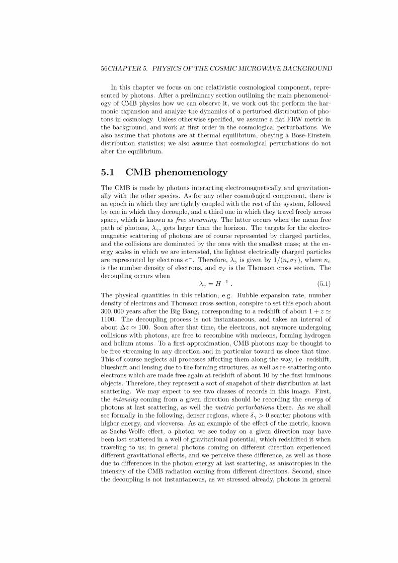
56CHAPTER 5. PHYSICS OF THE COSMICMICROWAVE BACKGROUND
In this chapter we focus on one relativistic cosmological component, repre-sented by photons. After a preliminary section outlining the main phenomenol-ogy of CMB physics how we can observe it, we work out the perform the har-monic expansion and analyze the dynamics of a perturbed distribution of pho-tons in cosmology. Unless otherwise specified, we assume a flat FRW metric inthe background, and work at first order in the cosmological perturbations. Wealso assume that photons are at thermal equilibrium, obeying a Bose-Einsteindistribution statistics; we also assume that cosmological perturbations do notalter the equilibrium.
5.1 CMB phenomenology
The CMB is made by photons interacting electromagnetically and gravitation-ally with the other species. As for any other cosmological component, there isan epoch in which they are tightly coupled with the rest of the system, followedby one in which they decouple, and a third one in which they travel freely acrossspace, which is known as free streaming. The latter occurs when the mean freepath of photons, λγ , gets larger than the horizon. The targets for the electro-magnetic scattering of photons are of course represented by charged particles,and the collisions are dominated by the ones with the smallest mass; at the en-ergy scales in which we are interested, the lightest electrically charged particlesare represented by electrons e−. Therefore, λγ is given by 1/(neσT ), where neis the number density of electrons, and σT is the Thomson cross section. Thedecoupling occurs when
λγ = H−1 . (5.1)
The physical quantities in this relation, e.g. Hubble expansion rate, numberdensity of electrons and Thomson cross section, conspire to set this epoch about300, 000 years after the Big Bang, corresponding to a redshift of about 1 + z '1100. The decoupling process is not instantaneous, and takes an interval ofabout ∆z ' 100. Soon after that time, the electrons, not anymore undergoingcollisions with photons, are free to recombine with nucleons, forming hydrogenand helium atoms. To a first approximation, CMB photons may be thought tobe free streaming in any direction and in particular toward us since that time.This of course neglects all processes affecting them along the way, i.e. redshift,blueshuft and lensing due to the forming structures, as well as re-scattering ontoelectrons which are made free again at redshift of about 10 by the first luminousobjects. Therefore, they represent a sort of snapshot of their distribution at lastscattering. We may expect to see two classes of records in this image. First,the intensity coming from a given direction should be recording the energy ofphotons at last scattering, as well the metric perturbations there. As we shallsee formally in the following, denser regions, where δγ > 0 scatter photons withhigher energy, and viceversa. As an example of the effect of the metric, knownas Sachs-Wolfe effect, a photon we see today on a given direction may havebeen last scattered in a well of gravitational potential, which redshifted it whentraveling to us; in general photons coming on different direction experienceddifferent gravitational effects, and we perceive these difference, as well as thosedue to differences in the photon energy at last scattering, as anisotropies in theintensity of the CMB radiation coming from different directions. Second, sincethe decoupling is not instantaneous, as we stressed already, photons in general
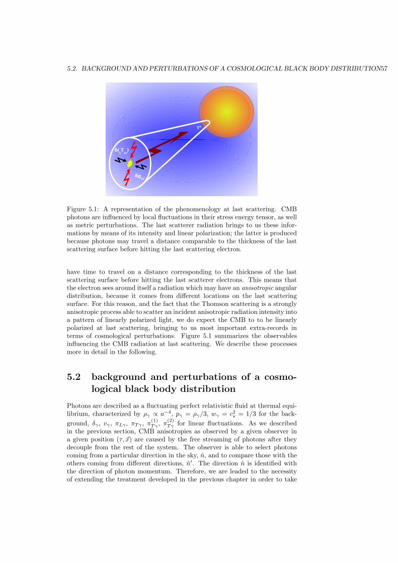
5.2. BACKGROUNDAND PERTURBATIONS OF A COSMOLOGICAL BLACK BODYDISTRIBUTION57
Figure 5.1: A representation of the phenomenology at last scattering. CMBphotons are influenced by local fluctuations in their stress energy tensor, as wellas metric perturbations. The last scatterer radiation brings to us these infor-mations by means of its intensity and linear polarization; the latter is producedbecause photons may travel a distance comparable to the thickness of the lastscattering surface before hitting the last scattering electron.
have time to travel on a distance corresponding to the thickness of the lastscattering surface before hitting the last scatterer electrons. This means thatthe electron sees around itself a radiation which may have an anisotropic angulardistribution, because it comes from different locations on the last scatteringsurface. For this reason, and the fact that the Thomson scattering is a stronglyanisotropic process able to scatter an incident anisotropic radiation intensity intoa pattern of linearly polarized light, we do expect the CMB to to be linearlypolarized at last scattering, bringing to us most important extra-records interms of cosmological perturbations. Figure 5.1 summarizes the observablesinfluencing the CMB radiation at last scattering. We describe these processesmore in detail in the following.
5.2 background and perturbations of a cosmo-logical black body distribution
Photons are described as a fluctuating perfect relativistic fluid at thermal equi-librium, characterized by ργ ∝ a−4, pγ = ργ/3, wγ = c2s = 1/3 for the back-
ground, δγ , vγ , πLγ , πTγ , π(1)Tγ , π
(2)Tγ for linear fluctuations. As we described
in the previous section, CMB anisotropies as observed by a given observer ina given position (τ, ~x) are caused by the free streaming of photons after theydecouple from the rest of the system. The observer is able to select photonscoming from a particular direction in the sky, n, and to compare those with theothers coming from different directions, n′. The direction n is identified withthe direction of photon momentum. Therefore, we are leaded to the necessityof extending the treatment developed in the previous chapter in order to take
58CHAPTER 5. PHYSICS OF THE COSMICMICROWAVE BACKGROUND
into account the momentum of particles. As we see now, this is easily doneexploiting the assumption thermal equilibrium.
In Minkowski spacetime, photons are characterized by a momentum obeyingthe massless condition
0 = pµpµ = −(p0)2 + |~p|2 , (5.2)
where their energy E is identified as the time component of the quadri-momentum,p0. Thus, at thermal equilibrium and temperature T , the number density dnγof photons with energy E and momentum ~p is that of a black body obeying theBose-Einstein distribution d with gγ = 2 degrees of freedom:
dnγ = d(E, T )d3p =gγ
exp(E/kBT )− 1d3p . (5.3)
It may be verified that in our units, ~ = c = 1, this has indeed the dimen-sions of the inverse of a volume. As usual, the number density of photons whenall momenta are counted is simply the integral of (5.3). When multiplied bythe energy and momentum, (5.3) gives the energy density ργ and the pressurepγ = ργ/3, respectively.We now need to bring this into the framework of the general relativistic cosmo-logical perturbation theory. The first step consists in choosing an appropriatequantity representing the energy E above. Due to the symmetry of the FRWmetric, yielding 0 = a2(−(p0)2 + |~p|2), one may safely define the backgroundenergy of photons in cosmology as
E(τ) =√gii(pi)2 =
√a2|~p|2 =
√−g00(p0)2 = a2(p0)2 , (5.4)
where we emphasize that E depends on time as any background quantity incosmology. Let us now consider perturbations. From (5.4), δE is activatedboth by δgµν and δpµ; it is important to realize that they are not independentbecause of the massless constraint. Imposing δ(pµp
µ) = 0 yields
2p0δp0 − h00(p0)2 = −2h0ip0pi + 2piδpi + hijp
ipj , (5.5)
which represents a relation between the perturbed photon momentum and themetric fluctuations δgµν = a2hµν defined in the previous chapter, expressedin a gauge independent formalism. It is now convenient to adopt a specificgauge, which is not the gauge invariant one, simplifying the treatment whichfollows. That is the Newtonian one defined in (3.104). The off diagonal terms
in (5.5) disappear. For vector-type perturbations, only the h(±1)0i elements are
non-zero. Of course, h(±2)ij is generally non-zero as it represents the amplitude of
gravitational waves and is unaffected by gauge transformations. Both left andright hand sides represent the fluctuations δE which may be obtained perturbing(5.4). This leads us to a perturbed expression for the black body dustributionfunction in (5.3): by replacing E with E + δE one obtains
gγ
exp(E+δEkBT
)− 1
=gγ
exp[
EkBT
(1−Θ)]− 1
, (5.6)
where Θ = −δE/E has been defined and may be interpreted as the first ordercorrection to the temperature T which would lead to an equivalent perturbation
5.2. BACKGROUNDAND PERTURBATIONS OF A COSMOLOGICAL BLACK BODYDISTRIBUTION59
to the black body spectrum if E is unperturbed. At first order, one obtains
δd = −ΘE
kBT
d
d(E/kBT )
[gγ
exp(E/kBT )− 1
]=
= ΘE
kBT
gγ exp(E/kBT )
[exp(E/kBT )− 1]2. (5.7)
From the relations above, it is easy to see that δE or Θ depend on a genericspacetime point (τ, ~x) through δgµν , as well as on the photon momenta pµ. Aswe anticipated at the beginning of this chapter, we do not allow Θ to dependon E , as that would represent a distortion of the black body spectrum, i.e. thebreaking of thermal equilibrium. Within this assumption, the perturbed spec-trum is still black blackbody for any spacetime position and photon propagationdirection. Defining ~p = En, one has
−δEE
(τ, ~x, n) = Θ(τ, ~x, n) . (5.8)
It is important at this point to estabilish a connection with the perturbativeanalysis developed in the previous chapter. The perturbed energy density isgiven by
ργ = ργ + δργ =
∫E(d+ δd)d3p . (5.9)
By exploiting (5.7) it is easy to see that
ργ(τ)− ργ(τ, ~x)
ργ(τ)= δγ(τ, ~x) = 4
∫Θ(τ, ~x, n)
4πdΩn = 4Θ0 , (5.10)
where all arguments have been made explicit. This means that the perturbationto the energy density of photons is four times the monopole of the temperaturefluctuations, represented by Θ0 above, consistenltly with the Stephan Boltz-mann law. The photon momentum density δγT
i0, including both scalar-type
and vector-type components, (ργ + pγ)(viγ + vi(±1)γ ) is given by
(ργ + pγ)(viγ + vi(±1)γ )(τ, ~x) =
ργπ
∫Θ(τ, ~x, n) cos θndΩn , (5.11)
where θn is the angle between n and the polar axis, which may be chosen tocoincide with the direction i; using wγ = 1/3 one gets
(viγ + vi(1)γ )(τ, ~x) =
3
4π
∫Θ(τ, ~x, n) cos θndΩn = Θ1(τ, ~x) , (5.12)
where the last equality defines the dipole of Θ The scalar-type and vector-typecomponents may be obtained by expanding the expression above in the Fourierspace, using the appropriate expansion set, Y (~k, ~x) and Y ±1(~k, ~x), respectively.In the same way, using the black body definition of pressure, it is easy to verifythat
πLγ =1
3δγ , (5.13)
still because Θ does not depend on E. Finally, the anisotropic stress is given by
pγ(πTγ + π(±1)Tγ + π
(±2)Tγ )(τ, ~x) =
∫E5
kBT
dE
[exp(E/kBT )− 1]2·
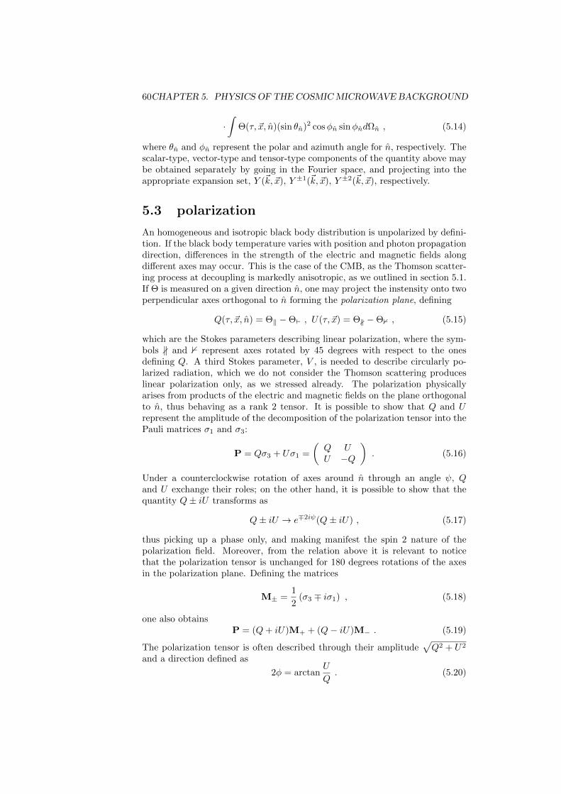
60CHAPTER 5. PHYSICS OF THE COSMICMICROWAVE BACKGROUND
·∫
Θ(τ, ~x, n)(sin θn)2 cosφn sinφndΩn , (5.14)
where θn and φn represent the polar and azimuth angle for n, respectively. Thescalar-type, vector-type and tensor-type components of the quantity above maybe obtained separately by going in the Fourier space, and projecting into theappropriate expansion set, Y (~k, ~x), Y ±1(~k, ~x), Y ±2(~k, ~x), respectively.
5.3 polarization
An homogeneous and isotropic black body distribution is unpolarized by defini-tion. If the black body temperature varies with position and photon propagationdirection, differences in the strength of the electric and magnetic fields alongdifferent axes may occur. This is the case of the CMB, as the Thomson scatter-ing process at decoupling is markedly anisotropic, as we outlined in section 5.1.If Θ is measured on a given direction n, one may project the instensity onto twoperpendicular axes orthogonal to n forming the polarization plane, defining
Q(τ, ~x, n) = Θ‖ −Θ` , U(τ, ~x) = Θ∦ −Θ0 , (5.15)
which are the Stokes parameters describing linear polarization, where the sym-bols ∦ and 0 represent axes rotated by 45 degrees with respect to the onesdefining Q. A third Stokes parameter, V , is needed to describe circularly po-larized radiation, which we do not consider the Thomson scattering produceslinear polarization only, as we stressed already. The polarization physicallyarises from products of the electric and magnetic fields on the plane orthogonalto n, thus behaving as a rank 2 tensor. It is possible to show that Q and Urepresent the amplitude of the decomposition of the polarization tensor into thePauli matrices σ1 and σ3:
P = Qσ3 + Uσ1 =
(Q UU −Q
). (5.16)
Under a counterclockwise rotation of axes around n through an angle ψ, Qand U exchange their roles; on the other hand, it is possible to show that thequantity Q± iU transforms as
Q± iU → e∓2iψ(Q± iU) , (5.17)
thus picking up a phase only, and making manifest the spin 2 nature of thepolarization field. Moreover, from the relation above it is relevant to noticethat the polarization tensor is unchanged for 180 degrees rotations of the axesin the polarization plane. Defining the matrices
M± =1
2(σ3 ∓ iσ1) , (5.18)
one also obtainsP = (Q+ iU)M+ + (Q− iU)M− . (5.19)
The polarization tensor is often described through their amplitude√Q2 + U2
and a direction defined as
2φ = arctanU
Q. (5.20)
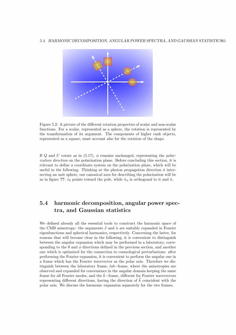
5.4. HARMONIC DECOMPOSITION, ANGULAR POWER SPECTRA, ANDGAUSSIAN STATISTICS61
Figure 5.2: A picture of the different rotation properties of scalar and non-scalarfunctions. For a scalar, represented as a sphere, the rotation is represented bythe transformation of its argument. The components of higher rank objects,represented as a square, must account also for the rotation of the shape.
If Q and U rotate as in (5.17), φ remains unchanged, representing the polar-ization direction on the polarization plane. Before concluding this section, it isrelevant to define a coordinate system on the polarization plane, which will beuseful in the following. Thinking at the photon propagation direction n inter-secting an unit sphere, our canonical axes for describing the polarization will beas in figure ??: eθ points toward the pole, while nφ is orthogonal to it and n.
5.4 harmonic decomposition, angular power spec-tra, and Gaussian statistics
We defined already all the essential tools to construct the harmonic space ofthe CMB anisotropy: the arguments ~x and n are suitably expanded in Fouriereigenfunctions and spherical harmonics, respectively. Concerning the latter, forreasons that will become clear in the following, it is convenient to distinguishbetween the angular expansion which may be performed in a laboratory, corre-sponding to the θ and φ directions defined in the previous section, and anotherone which is optimized for the connection to cosmological perturbations: afterperforming the Fourier expansion, it is convenient to perform the angular one ina frame which has the Fourier wavevector as the polar axis. Therefore we dis-tinguish between the laboratory frame, lab−frame, where the anisotropies areobserved and expanded for convenience in the angular domain keeping the sameframe for all Fourier modes, and the k−frame, different for Fourier wavevectorsrepresenting different directions, having the direction of ~k coincident with thepolar axis. We discuss the harmonic expansion separately for the two frames.
62CHAPTER 5. PHYSICS OF THE COSMICMICROWAVE BACKGROUND
5.4.1 lab−frame
Spacetime dependence and harmonic expansion are completely independent.Therefore, for any given position x, the angular expansion of Θ, Q± iU is
Θ(τ, ~x, n) =∑lm
Θlm(τ, ~x)Ylm(n) ,
(Q± iU)(τ, ~x, n)M± =∑lm
(Q± iU)lm(τ, ~x)±2Ylm(n)M± , (5.21)
where we notice that Q± iU has been expanded in tensor spherical harmonics,indicated as ±2Ylm(n), being the components of a rank 2 tensor; figure 5.2 rep-resents the difference in the angular pattern when scalar and non-scalar objectsare rotated, represented as a ball and a square, respectively: for the ball, thecoordinate transformation is enough; for the square, its shape rotates as well sothat a set of spherical harmonics corresponding to higher rank objects is neces-sary.The expansion coefficients in (5.21) fully describe the CMB observables; how-ever, for polarization, a simple but most important step for their connectionwith cosmological perturbations has to be made. Indeed, the combinations
Y ElmME =1
2
(2Ylm bfM+ + 2Ylm bfM−
),
Y BlmMB =1
2
(2Ylm bfM+ − 2Ylm bfM−
)(5.22)
pick up a (−1)l and (−1)l+1, respectively, under transformations n → −n.The notation has been chosen because it is possible to show that these are theappropriate parity relations for the angular distribution of the electric ~E andmagnetic ~B fields, generated by the gradient of a scalar potential, and the curlof a vector one, respectively. The polarization tensor is described through
P = (Q+ iU)M+ + (Q− iU)M− =∑lm
(ElmYElmME +BlmY
BlmMB) , (5.23)
where
Elm =1
2[(Q+ iU)lm + (Q− iU)lm] ,
Blm =1
2i[(Q+ iU)lm − (Q− iU)lm] . (5.24)
As we see in the next sub-section, the E modes are excited by all kinds of cos-mological perturbations, while the B modes are activated by non-scalar ones,only.It is now straightforward to define the angular power spectrum of CMB anisotropies:at any spacetime location x, the angular power spectra of CMB anisotropies aredefined as
CΘΘl (τ, ~x) =
1
2l + 1
∑m
|Θlm(τ, ~x)|2 ,
CΘEl (τ, ~x) =
1
2l + 1
∑m
Θlm(τ, ~x)E∗lm(τ, ~x) ,
5.4. HARMONIC DECOMPOSITION, ANGULAR POWER SPECTRA, ANDGAUSSIAN STATISTICS63
CΘBl (τ, ~x) =
1
2l + 1
∑m
Θlm(τ, ~x)B∗lm(τ, ~x) ,
CEEl =1
2l + 1
∑m
|Elm(τ, ~x)|2 ,
CBBl =1
2l + 1
∑m
|Blm(τ, ~x)|2 .,
CEBl =1
2l + 1
∑m
Elm(τ, ~x)B∗lm(τ, ~x) . (5.25)
Although this represents a lossy compression of the CMB observables, as forexample the phases of the aΘ
lm coefficients are lost, it is convenient from thepoint of view of a statistical description of those. If each lm coefficient is aGaussian variable with known variance, no physical information is coded intothe phases of CMB anisotropies, so that the compression (5.25) is lossless:
< ΘlmΘl′m′ >= CΘΘl δll′δmm′ , < ΘlmEl′m′ >= CΘE
l δll′δmm′ ,
< ElmE∗l′m′ >= CEEl δll′δmm′ , < BlmBl′m′ >= CBBl δll′δmm′ ,
< ΘlmBl′m′ >= 0 , < ElmB∗l′m′ >= 0 , (5.26)
The vanishing spectra above are due to the absence of parity violations in theinteractions of the CMB with other particles. It is important to distinguishbetween the angular power spectra (5.25), defined on the sky, i.e. on a givenrealization of the system, and those in (5.26), which are supposed to describe theaveraged variance of the anisotropy power over the whole Gaussian statistics.
5.4.2 k−frame
We first provide a basis of expansion for total intensity anisotropies, representedby the temperature fluctuation Θ(τ, ~x, n). We already formalized the Fourier
harmonic modes Y (~k, ~x), which are simply plane waves, ei~k·~x, in our hypothesis
of flat FRW. They may be used to describe the Fourier decomposition:
Θ(τ, ~x, n) =
∫Θ(τ,~k, n)Y (~k, ~x)d3k . (5.27)
Being in the k−frame means performing the angular expansion taking the kdirection as the polar axis. Therefore, our expansion set for (5.8) is
Glm(~x,~k, n) = (−i)lY (~k, ~x)
√4π
2l + 1Ylm(nk) (5.28)
where Ylm(nk) are the usual spherical harmonics, the subscript indicates that n
is expressed in the k−frame, and the constants in front are purely conventional.The harmonic coefficients of Θ along the basis (5.28) are given by
Θlm(τ,~k) =
∫d3x
∫dΩknΘ(τ, ~x, n)Glm(~k, ~x, n) , (5.29)
64CHAPTER 5. PHYSICS OF THE COSMICMICROWAVE BACKGROUND
and the full expansion of Θ is
Θ(τ, ~x, n) =
∫ ∑lm
Θlm(τ,~k)Glm(~x,~k, n)d3k . (5.30)
In the following, we explicitate the arguments of the various functions only ifnecessary.For polarization, the expansion proceeds conceptually as outlined in the previ-ous sub-section; the E and B modes in the k−frame are formally identical to(5.22,5.24), the only difference being the polar axis aligned with k; their par-
ity properties are of course respected in the k−frame as well. Therefore, theexpansion set for polarization is given by
±2Glm(~x,~k, n) = (−i)lY (~k, ~x)
√4π
2l + 1±2Ylm(nk)Mk
± , (5.31)
where again the the subscript indicates that n and the Pauli matrices are ex-pressed in the k−frame. At this point it is straightforward to define the expan-sion set for the E and B modes; following (5.22), they are given by
GElm =1
2(2Glm + −2Glm) , GBlm =
1
2(2Glm − −2Glm) , (5.32)
so that the polarization tensor is given by
P(τ, ~x, n) = (Q+ iU)(τ, ~x, n)M+ + (Q− iU)(τ, ~x, n)M− =
=
∫d3k
∑lm
[Elm(τ,~k)GElm(nk)M
~kE +Blm(τ,~k)GBlm(nk)M
~kB
], (5.33)
where all arguments have been made explicit. It is now convenient to anticipatean aspect that would become clear from the following discussion, but has adirect relevance for the harmonic modes in the k−frame, which are discussedhere. In the Boltzmann equation to be discussed next, the metric perturbationsin the Fourier space, i.e. expressed by their amplitude multiplied by Y , Yi, Yij
for scalar-type components, Y(±1)i , Y
(±1)ij for vector-type components, Y
(±2)ij for
tensor-type components, appear contracted with ni or ninj , where the latter arethe components of n. In the k−frame, the latter contraction have an immediateexpression in terms of spherical harmonics, thus making an explicit and one toone connection with the harmonic modes Glm. For scalar-type perturbations,Y ∝ G00, niYi ∝ G10, ninjYij ∝ G20. This means that scalar-type fluctuations
excite only modes with m = 0 in the k−frame, and with l ≤ 2. For vector-type
perturbations, niY(±1)i ∝ G1±1, ninjY
(±1)ij ∝ G2±1. This means that vector-
type fluctuations excite only modes with m = ±1 in the k−frame, and with
l ≤ 2. Finally, For tensor-type perturbations, ninjY(±2)ij ∝ G2±2, i.e. they
excite only modes with m = ±2 in the k−frame, and with l ≤ 2.
5.5 Boltzmann equation
The Boltzmann equation describes the dynamics of distribution functions, rep-resented by the perturbed black body spectrum in our case, d. The latter is
5.6. GRAVITATIONAL SCATTERING 65
affected by two processes, namely gravity and Thomson scattering. Therefore,by propagating the total time derivative in all arguments, the Boltzmann equa-tion for the CMB may be written as
dd
dτ= ˙d+
∂d
∂xidxi
dτ+∂d
∂E
dE
dτ+
∂d
∂nidni
dτ= G+ C , (5.34)
where the two terms on the right hand side represent the gravitational andThomson scattering, respectively, and as usual the bar indicates backgroundplus perturbations. A first simplification concerns the first term: since thedistribution does not depend explicitely on time, that is absent. As we shallsee later, there is no scattering process at the background level; in other words,the strength of the Thomson scattering is not high enough to undermine theexistence of a cosmological homogeneous and isotropic background, C = 0.Therefore, since the unperturbed Bose Einstein statistics depends only on E,the background component of (5.34) reduces to
E = G , (5.35)
where the term describing the gravitational effect at the background level hasbeen re-defined appropriately. At the perturbation level, equation (5.34) deter-mines the evolution of Θ(τ, ~x, n). Since the Bose Einstein statistics depends onthe position only at the perturbation level, the second term in (5.34) is firstorder. Moreover, the term dxi/dτ may be directly related to the photon propa-gation direction: if as we see in the nect section η is the affine parameter alongthe photon geodesic, dxi/dτ = (dxi/dη) · (dη/dτ) = pi/p0 = ni. Moreover, in aflat FRW background the last term in (5.34) contributes only to second orderand we neglect it. Note that if the background were not flat, then ni 6= 0 atthe background level, and the last term in (5.34) would definitely contribute atfirst order. Therefore, exploiting the perturbed expression (5.7) the perturbedBoltzmann equation may be written as
Θ + n · ~∇Θ = δG+ δCΘ , (5.36)
where again the gravitational and Thomson scattering terms have been re-defined appropriately, and shall be evaluated in the following.
5.6 gravitational scattering
The time derivative of E in (5.34) is determined by the the geodesics propagationof photons in a linearly perturbed FRW metric. As we have seen in chapter ??,the latter may be written as
gµν = a2(γµν + hµν) , (5.37)
where hµν represents the perturbation. In the following, we shall choose theNewtonian gauge, where the non-null terms in the Fourier space are
h00 = 2AY , h0i = B±1Y(±1)i , hij = 2HLY δij + 2H±2
T Y(±2)ij , (5.38)
and were defined in the previous chapter. Moreover, in this section we workout the geodesic propagation for a diagonal perturbation, h0i = hi6=j = 0, as
66CHAPTER 5. PHYSICS OF THE COSMICMICROWAVE BACKGROUND
appropriate in the case of scalar-type perturbations. In the end we quote thecomplete result. The quadrimomentum pµ = dxµ/dτ of photons obeys therelation pµpµ = 0, which holds both for the background and perturbations:
(p0)2 = (~p)2 , δgµνpµpν + 2gµνp
µδpν = 0 . (5.39)
The geodesic equation is
d2xµ
dξ2+ Γµνρ
dxν
dξ
dxρ
dξ= 0 , (5.40)
where ξ represents the affine parameter along the path. The latter may bechosen such that
p0 =dx0
dξ, ~p =
d~x
dξ= p0 d~x
dτ, (5.41)
where we used the fact that x0 is the conformal time. The Christoffel symbolsare
Γµνρ =1
2gµµ
′(gµ′ν,ρ + gµ′ρ,ν − gνρ,µ′) , (5.42)
where the perturbed part is
δΓµνρ =1
2δgµµ
′(gµ′ν,ρ + gµ′ρ,ν − gνρ,µ′)+
+1
2gµµ
′(δgµ′ν,ρ + δgµ′ρ,ν − δgνρ,µ′) . (5.43)
Let us concentrate now on the behavior of the µ = 0 component, consideringthe background first. From (5.42) it may be seen that the only non-zero com-ponents of the Christoffel symbols in a flat FRW are Γ0
00 = Γ0ii = H. Therefore,
(5.40,5.41,5.47) givedp0
dτ+ 2Hp0 = 0 , (5.44)
which implies p0 ∝ a−2, and therefore E =√−g00(p0)2 =
√gii(pi)2 ∝ a−1;
this is the well known redshift of the photon energy in an expansing background.Let us focus on perturbations now. Using (5.41, )the perturbed component of(5.40) with µ = 0 is
δp0 dp0
dτ+ p0 dδp
0
dτ+ δΓ0
νρpνpρ + 2Γ0
νρδpνpρ . (5.45)
Using the background components of the Christoffel symbols and (5.44), theexpression above simplifies:
p0 dδp0
dτ+ δΓ0
νρpνpρ + 2H~p · δ~p . (5.46)
Moreover, from (5.47) and using our hypothesis of diagonal hµν , we obtain
~p · δ~p = −1
2h00(p0)2 +
1
2hii(p
i)2 + p0δp0 . (5.47)
Moreover, from (5.43) it is easy to see that if hµν is diagonal, the only non-vanishing terms of the perturbed Christoffel symbols are δΓ0
00 , δΓ0ii, δΓ
00i. Using
5.7. THOMSON SCATTERING 67
the relation δg00 = −δg00/a4 which may be obtained from g00 = g0µg0ν gµν ,
their expressions are
δΓ000 = −1
2h00,0 ,
δΓ0ii = H(h00 + hii) +
1
2hii,0 , δΓ
00i = −1
2h00,i . (5.48)
Using (5.47,5.48), the perturbed geodesic equation becomes
dδp0
dτ+ 2Hp0δp0 − 1
2h00,0p
0 +1
2hii,0p
0(ni)2 − h00,ip0ni = 0 , (5.49)
where we used the fact that ni = dxi/dτ = pi/p0. Finally, the variation ofE2 = −g00(p0)2 gives 2EδE = −a2h00(p0)2 + 2a2p0δp0 = −E2(h00 − 2δp0/p0)which implies
δE
E= −1
2h00 +
δp0
p0. (5.50)
Therefore, from (5.49) and noticing that (1/p0)dδp0/dτ+2Hp0δp0 = d(δp0/p0)/dτ ,one has
d(δE/E)
dτ= −1
2hii,0(ni)2 +
1
2h00,in
i . (5.51)
The result for arbitrary hµν , involving non-diagonal scalar-type, vector-type andtensor-type perturbations, is
−dΘ
dτ=d(δE/E)
dτ= −1
2hij,0n
inj +1
2h00,in
i − h0i,0ni . (5.52)
These relations determine the δG term in (5.36).
5.7 Thomson scattering
The CMB temperature today is T ' 3K which corresponds to about 1/4000 eVin energy units. At decoupling, this corresponds to the eV. At these energies,the relevant cosmological species are represented by photons γ, free electronse− in non-relativistic regime because me ' 900 MeV, hydrogen and heliumatoms and nuclei, plus many other particles, interacting at most weakly with theformer classes, e.g. neutrinos ν, dark matter. The most relevant interaction forphotons and these energies and lower is Compton scattering onto non-relativisticelectrons, indicated by the following relation
e−(qµ) + γ(pµ)→ e−(qµ′) + γ(pµ′) , (5.53)
where qµ, pµ, qµ′, pµ′ are the electron and photon incoming and outcomingquadri-momenta, respectively.We are interested in the change in the photon distribution d from Comptonscattering; it will be necessary for a while to consider the electron distributionfunction, de. In the spacetime point x, in the time interval dt, a number of elec-tron and photon states given by the product between de(x, q
µ′) and d(x, pµ′),respectively, determine an outgoing photon with quadri-momentum pµ corre-sponding to our variables E and n, and therefore an increase in d. At thesame time, a number of states given by the product between de(x, q
µ) and
68CHAPTER 5. PHYSICS OF THE COSMICMICROWAVE BACKGROUND
d(x, pµ) determines an outgoing photon with momentum pµ′ and a decrease in
d. Schematically, the term C in the Boltzmann equation (5.34) may be writtenas
C =∑
qµ,qµ′,pµ′
T [de(x, qµ′)d(x, pµ′)− de(x, qµ)d(x, pµ)] , (5.54)
where T is a constant and indicates the strength of the interaction. Let usnow make some consideration on the expression above, which simplify the cal-culations below. First of all, as we anticipated above, due to the magnitude ofthe Thomson scattering cross section, there is no background term in (5.54),C = 0. Moreover, at energies comparable or lower than the eV, the energytransfer between photons as well as the electrom momentum are small quan-tities with respect to the mass of electrons. Therefore the photon energy ex-change p0′ − p0 = E′ − E in (5.54) as well as the electron kinetic energy maybe treated perturbatively; in the present analysis, we only keep terms whichare at first order in cosmological perturbations or photon energy exchange orelectron momentum. Moreover, due to the small spacetime scales involved bythe interaction, we approximate the metric as Minkowskian, and the energy ofphotons is simply given by E = |~p|, while that of electrons by Ee =
√m2e + |~q|2.
More simplifications may be found by looking at first order in (5.53); makingthe background and fluctiation terms in the electron energy distribution explicit,one gets
δC =∑
qµ,qµ′,pµ′
T [δde(x, qµ′)d(x, pµ′) + de(x, qµ′)d(x, pµ′)]−
−[δde(x, qµ)]d(x, pµ)− de(x, qµ)d(x, pµ)] . (5.55)
The background photon distribution depends on the photon energy only. There-fore, the difference between the first and third term is first order in the photonenergy exchange as well as in cosmological perturbations, and may be neglectedin our approximations. This allows us to use the background electron densitydistribution only. Writing the sum in (5.55) appropriately for electromagnetism,one gets
δC =
∫d3q
2Ee
∫d3q′
2E′e
∫d3p′
2E′· TE·
·δ(E + Ee − E′ − E′e)δ3(~p+ ~q − ~p′ − ~q′)[d′ed(x, pµ′)− ded(x, pµ)] , (5.56)
where we simplified the notation indicating with a ′ the quantities dependingon pµ′, qµ′. In our approximation of small energy exchange and electron mo-mentum, the electron energy in the denominator of (5.56) may be replaced byme. With that we may perform the integration over ~q′, which gives
δC =1
4m2e
∫d3q
∫d3p′
2E′TEδ(E + Ee − E′ − E′e)·
·[d′ed(x, pµ′)− ded(x, pµ)] . (5.57)
The argument of the Dirac delta above may be treated as follows. In the non-relativistic regime, the energy of electrons is given by me + |~q|2/2me; theirdifference in (5.57) is given by
|~q|2
2me− |~q + ~p− ~p′|2
2me' ~q(~p′ − ~p)
me, (5.58)
5.7. THOMSON SCATTERING 69
so that the Dirac delta becomes
δ
[E − E′ + ~q(~p′ − ~p)
me
]. (5.59)
The next simplification concerns the last term in (5.57). Indeed, the differenceis first order in E′ −E or Θ; therefore, the background electron distribution d′emay be actually computed on q0 and factored out of the integral:
δC =1
4m2e
∫d3qde·
·∫d3p′
2E′TEδ
[E − E′ + ~q(~p′ − ~p)
me
][d(x, pµ′)− d(x, pµ)] . (5.60)
In order to proceed we need to explicitate T . The Thomson scattering isanisotropic, in the sense that the intensity of the emitted light depends on theangular distribution of the incident radiation. Moreover, an unpolarized butanisotropic incoming radiation is linearly polarized during scattering, due tothe motion of the electron, following the direction of the incoming electric field.As we stressed in section 5.1, at decoupling the photons hit the last scattererelectron with an anisotropic intensity, and therefore we do expect a linear polar-ization in the CMB radiation. We do not take into account the polarization inthe present calculation, and we consider only the isotropic scattered component;at the end of this section, though, we give the complete result. The term in Twhich is responsible for the isotropic part of the scattered radiation is given by
T = (2/π)aσTm2e , (5.61)
where with all constants made explicit, the Thomson cross section σT is givenby 8πe4/3c4m2
e, and the factor a is simply due to the use of the conformal timein the time derivative of the photon distribution function, which is otherwisederived with respect to the ordinary time, dt = adτ . We expand the photondistributions d(x, pµ) and d(x, pµ′) to first order in Θ, and the second one tofirst order in E′ − E, too:
d(x, pµ) ' d(E)− E ∂d
∂EΘ , (5.62)
d(x, pµ′) ' d(E) +∂d
∂E(E′ − E)− E ∂d
∂EΘ′ . (5.63)
Any other term is second order in the photon momentum difference, or Θ, ortheir product, and we neglect it. Therefore, the term in between parenthesis in(5.60) becomes
d(x, pµ′)− d(x, pµ) ' ∂d
∂E(E′ − E)− E ∂d
∂E(Θ′ −Θ) . (5.64)
Note that the prime for Θ means that it is calculated on the incoming scatteringdirection, n′. Let us go back to the integral (5.60). First we pass to sphericalcoordinates for ~p′: d3p = E2′dE′dΩn′ . In the first integral, done with the firstterm in (5.64), the Dirac delta makes E′ −E calculated in ~q(~p′ − ~p)/me; in ourapproximations, keeping only first order terms in cosmological perturbations

70CHAPTER 5. PHYSICS OF THE COSMICMICROWAVE BACKGROUND
or photon energy transfer or electrum momentum, the latter term is simply~q(n′− n)E/me; the term in n′ gives zero when integrated over the directions onthe spheres, dΩn′ . The integral in d3q merely represents the definition of theaverage peculiar velocity of electrons:∫
d3qde~q
me= ne~ve . (5.65)
The second integral, done with the second term in (5.64), is already first orderin Θ, and may be calculated in E = E′. The integration in dΩ′ on the termdependent on Θ simply produces 4πΘ, as the latter is evaluated along n. Thesame integral applied on Θ′ produces the monopole term
4πΘ0 =
∫Θ′dΩn′ , (5.66)
which represents the monopole of the CMB temperature fluctuations, i.e. thedisplacement that the temperature has locally, in the spacetime point x, from itsaverage value. In this case, the integral in d3q simply produces the backgrounddensity of electrons, ne. Combining all these calculations together, the finalresult for the collision term from Compton scattering, in our approximations, is
δC = aneσTE∂d
∂E(Θ−Θ0 − n · ~ve) . (5.67)
This represents the Thomson scattering term in (5.34).We now give the complete result, including the polarization; it is a generalizationof (4.30), including mixing terms between Θ and Q ± iU . It is convenient todefine the differential optical depth
τ = aneσT , (5.68)
also equivalent to the inverse of the mean free path of photons via Thomsonscattering; again, the a factor in front is due to the fact that our time coordinateis dτ = dt/a. Moreover, it can be shown that the Coulomb interaction betweenelectron and protons is tight, so that the Let us first define the tensor C givenby
Cm =
Y2mY′2m −
√3/22Y
′2mY2m −
√3/2−2Y
′2mY2m
−√
6Y2m2Y′2m 32Y
′2m2Y2m 3−2Y
′2m2Y2m
−√
6Y ′2m−2Y2m 32Y′2m2Y2m 3−2Y
′2m−2Y2m
, (5.69)
where the prime indicates that a given quantity is evaluated on the incidentdirection n′; the Thomson scattering term for the Boltzmann equation expressedas in (5.36) is
δCΘ = −τ(Θ−Θ0 − n · ~vb)+
+τ
10
∫dΩn′
m=2∑m=−2
[Cm11Θ′ + Cm
12(Q+ iU)′ + Cm13(Q− iU)′] , (5.70)
where Θ0 is given by (5.10), and ~vb is the peculiar velocity of electrons. TheStokes parameters also undergo a dynamics due to the scattering process. Theresult is
˙(Q+ iU) + n · ~∇(Q+ iU) = δC(Q+iU) = −τ(Q+ iU)+
5.8. HARMONIC EXPANSION 71
+τ
10
∫dΩn′
m=2∑m=−2
[Cm21Θ′ + Cm
22(Q+ iU)′ + Cm23(Q− iU)′] ,
˙(Q− iU) + n · ~∇(Q− iU) = δCQ−iU = −τ(Q− iU)+
+τ
10
∫dΩn′
m=2∑m=−2
[Cm31Θ′ + Cm
32(Q+ iU)′ + Cm33(Q− iU)′] . (5.71)
where the friction caused by the scattering onto the Stokes parameters at eachspacetime location, as well as the amplification due to the incident anisotropicradiation are on the left and right hand side, respectively.
5.8 harmonic expansion
We now expand in spherical harmonics the perturbed Boltzmann equation, us-ing (5.52,5.82,5.71) and the k−frame decomposition in normal modes given by
(5.28,5.31). The first thing to notice is that the gradient term n · ~∇ becomes adipole term given by
in · ~k = i
√4π
3kY 0
1 . (5.72)
The l = 1, m = 0 spherical harmonic function above multiplies the ones in(5.28, 5.31), coupling different angular terms between each other. As we see now,this is actually the term which describes the free streaming, i.e. the projectionsof local anisotropies on larger and larger angular scales as time goes. Indeed,using the Clebsh-Gordan decomposition√
4π
3Y 0
1 sYml =
sκml√
(2l + 1)(2l − 1)sY
ml−1−
− ms
l(l + 1)sY
ml +
sκml+1√
(2l + 1)(2l + 3)sY
ml+1 , (5.73)
where
sκml =
√(l2 −m2)(l2 − s2)/l2 . (5.74)
Obviously the relations above hold for l ≥ m as for normal spherical harmonics;further conditions are l ≥ 1 if s = 0, for l ≥ 2 if s = 1 and for l ≥ 3 if s = 2. Inthe harmonic expression for the Boltzmann equation this means in particularthat the power is transferred dynamically from l to l + 1, i.e. during the freestreaming the anisotropy power at higher multipoles is populated. As we willsee in the next chapter, the anisotropy pattern we see today in the sky on allangular scales is essentially given by the monopole and dipole of the radiationfield at decoupling.With (5.73), the expansion of the Boltzmann equation (5.36) proceeds straight-forward with spherical harmonic algebra, becoming an infinite set of evolutionequations for the harmonic multipoles in Θ, Q± iU . Its expression for Θm
l is
Θml + τΘm
l − k(
0κml
2l − 1Θml−1 −
0κml+1
2l + 3Θml+1
)= Sml , (5.75)

72CHAPTER 5. PHYSICS OF THE COSMICMICROWAVE BACKGROUND
where the second term on the right hand side represents the friction due toThomson scattering, causing a damping of anisotropies because of the scat-tering itself, while the third one is the free streaming; source Sml collects allthe remaining anisotropic contributions from Thomson scattering, and all thosefrom the metric perturbations:
S00 = τΘ0
0 − HL , S01 = τ v0
b + kA , S02 = τP 0 , (5.76)
S±11 = τ v±1
b + B±1 , S±12 = τP±1 (5.77)
S±22 = τP±2 − H±2
T , (5.78)
Pm = Θm2
1
10−√
6
10Em2 . (5.79)
An analogous computation gives the evolution equations for the E and B modes:
Eml + τEml − k(
2κml
2l − 1Eml−1 −
2m
l(l + 1)Bml −
2κml+1
2l + 3Eml+1
)=
= −τ√
6Pmδl2 , (5.80)
Bml + τBml − k(
2κml
2l − 1Bml−1 +
2m
l(l + 1)Eml −
2κml+1
2l + 3Bml+1
)= 0 , (5.81)
In the next chapter, we shall analyse these equations outlining the main physicalphenomenology. On the other hand, several interesting features may be noticedbefore concluding. First, it is evident how the B modes may exist only fornon-scalar perturbations: the anisotropy power activates B only if m 6= 0 in(5.81). Second, the free streaming mixes E and B dynamically for each givenpair of l and m values, as it is represented by the presence of Bml in (5.80) andEml in (5.81). Third, the power transfer from total intensity to polarizationand back is represented by the Pm term defined in (5.79). As we shall see inthe next chapter, the anisotropy power is sourced by the metric perturbationsas well as the monopole and dipole in the Θ function; by free streaming, thepower is transferred to the quadrupole and the higher moments, activating thepolarization and projecting the whole anisotropy spectrum at higher and highermultipoles, as outlined above.
5.9 excercises
5.9.1 question about the dipole Thomson scattering
Consider the Thomson scattering contribution to the Boltzmann equation:
δC = aneσT [−(Θ−Θ0) + n · ~ve] . (5.82)
Write it explicitely for a temperature anisotropy term Θ possessing only amonopole and dipole. In the same hypotheses, find the relations between theΘ1m coefficients and ~ve such that the scattering amplitude vanishes, giving aphysical interpretation of the result. Show that if Θ possesses a quadrupole orhigher multipoles, then δC is always different from zero.
Chapter 6
Cosmic microwavebackground anisotropies
73
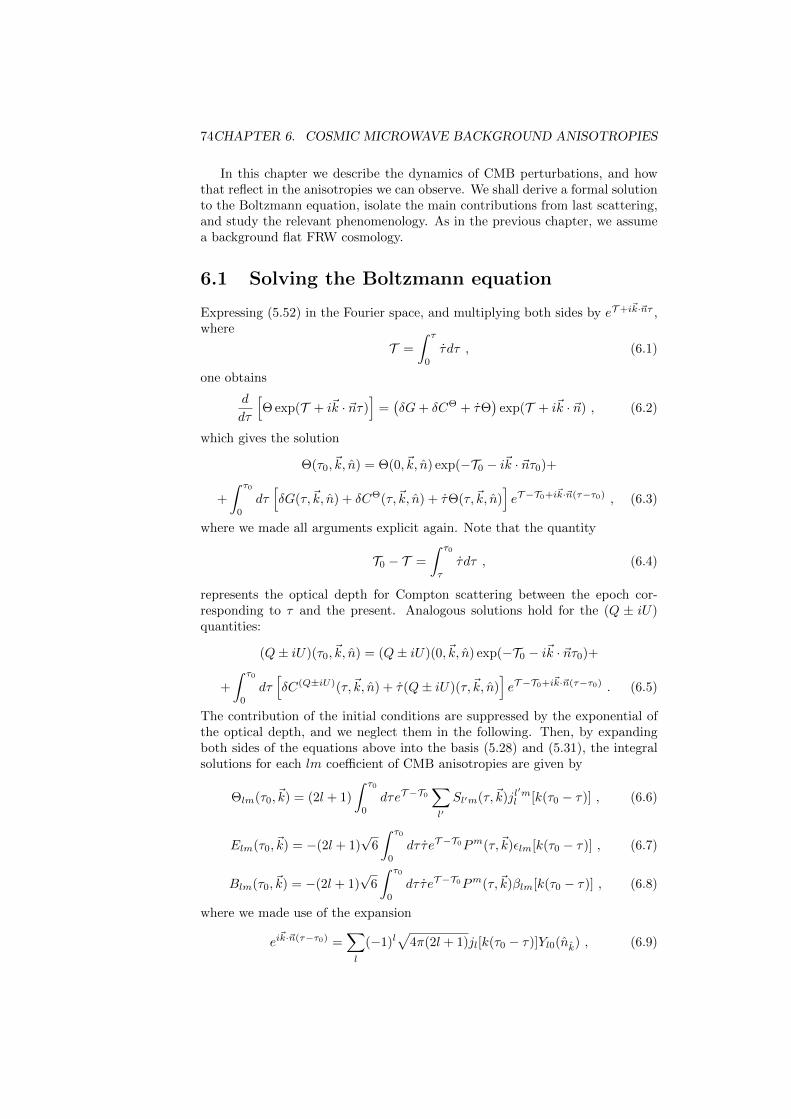
74CHAPTER 6. COSMIC MICROWAVE BACKGROUND ANISOTROPIES
In this chapter we describe the dynamics of CMB perturbations, and howthat reflect in the anisotropies we can observe. We shall derive a formal solutionto the Boltzmann equation, isolate the main contributions from last scattering,and study the relevant phenomenology. As in the previous chapter, we assumea background flat FRW cosmology.
6.1 Solving the Boltzmann equation
Expressing (5.52) in the Fourier space, and multiplying both sides by eT +i~k·~nτ ,where
T =
∫ τ
0
τ dτ , (6.1)
one obtains
d
dτ
[Θ exp(T + i~k · ~nτ)
]=(δG+ δCΘ + τΘ
)exp(T + i~k · ~n) , (6.2)
which gives the solution
Θ(τ0,~k, n) = Θ(0,~k, n) exp(−T0 − i~k · ~nτ0)+
+
∫ τ0
0
dτ[δG(τ,~k, n) + δCΘ(τ,~k, n) + τΘ(τ,~k, n)
]eT −T0+i~k·~n(τ−τ0) , (6.3)
where we made all arguments explicit again. Note that the quantity
T0 − T =
∫ τ0
τ
τ dτ , (6.4)
represents the optical depth for Compton scattering between the epoch cor-responding to τ and the present. Analogous solutions hold for the (Q ± iU)quantities:
(Q± iU)(τ0,~k, n) = (Q± iU)(0,~k, n) exp(−T0 − i~k · ~nτ0)+
+
∫ τ0
0
dτ[δC(Q±iU)(τ,~k, n) + τ(Q± iU)(τ,~k, n)
]eT −T0+i~k·~n(τ−τ0) . (6.5)
The contribution of the initial conditions are suppressed by the exponential ofthe optical depth, and we neglect them in the following. Then, by expandingboth sides of the equations above into the basis (5.28) and (5.31), the integralsolutions for each lm coefficient of CMB anisotropies are given by
Θlm(τ0,~k) = (2l + 1)
∫ τ0
0
dτeT −T0∑l′
Sl′m(τ,~k)jl′ml [k(τ0 − τ)] , (6.6)
Elm(τ0,~k) = −(2l + 1)√
6
∫ τ0
0
dτ τeT −T0Pm(τ,~k)εlm[k(τ0 − τ)] , (6.7)
Blm(τ0,~k) = −(2l + 1)√
6
∫ τ0
0
dτ τeT −T0Pm(τ,~k)βlm[k(τ0 − τ)] , (6.8)
where we made use of the expansion
ei~k·~n(τ−τ0) =
∑l
(−1)l√
4π(2l + 1)jl[k(τ0 − τ)]Yl0(nk) , (6.9)
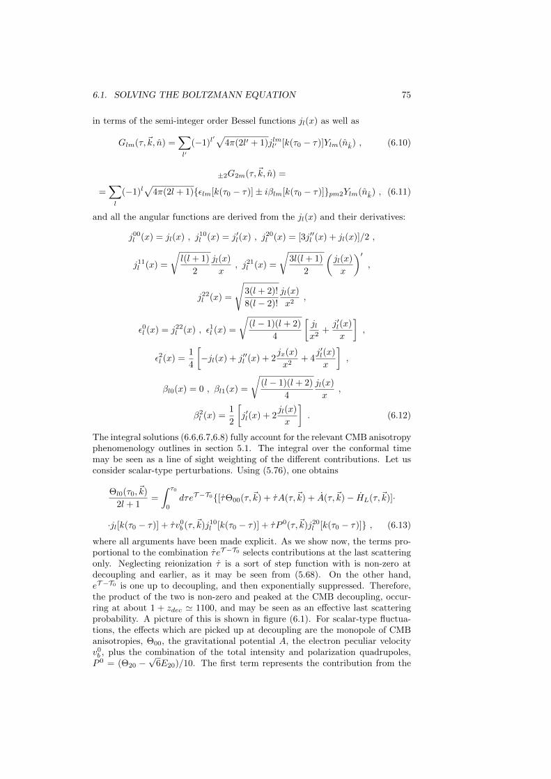
6.1. SOLVING THE BOLTZMANN EQUATION 75
in terms of the semi-integer order Bessel functions jl(x) as well as
Glm(τ,~k, n) =∑l′
(−1)l′√
4π(2l′ + 1)jlml′ [k(τ0 − τ)]Ylm(nk) , (6.10)
±2G2m(τ,~k, n) =
=∑l
(−1)l√
4π(2l + 1)εlm[k(τ0 − τ)]± iβlm[k(τ0 − τ)]pm2Ylm(nk) , (6.11)
and all the angular functions are derived from the jl(x) and their derivatives:
j00l (x) = jl(x) , j10
l (x) = j′l(x) , j20l (x) = [3j′′l (x) + jl(x)]/2 ,
j11l (x) =
√l(l + 1)
2
jl(x)
x, j21
l (x) =
√3l(l + 1)
2
(jl(x)
x
)′,
j22l (x) =
√3(l + 2)!
8(l − 2)!
jl(x)
x2,
ε0l (x) = j22l (x) , ε1l (x) =
√(l − 1)(l + 2)
4
[jlx2
+j′l(x)
x
],
ε2l (x) =1
4
[−jl(x) + j′′l (x) + 2
jx(x)
x2+ 4
j′l(x)
x
],
βl0(x) = 0 , βl1(x) =
√(l − 1)(l + 2)
4
jl(x)
x,
β2l (x) =
1
2
[j′l(x) + 2
jl(x)
x
]. (6.12)
The integral solutions (6.6,6.7,6.8) fully account for the relevant CMB anisotropyphenomenology outlines in section 5.1. The integral over the conformal timemay be seen as a line of sight weighting of the different contributions. Let usconsider scalar-type perturbations. Using (5.76), one obtains
Θl0(τ0,~k)
2l + 1=
∫ τ0
0
dτeT −T0[τΘ00(τ,~k) + τA(τ,~k) + A(τ,~k)− HL(τ,~k)]·
·jl[k(τ0 − τ)] + τ v0b (τ,~k)j10
l [k(τ0 − τ)] + τP 0(τ,~k)j20l [k(τ0 − τ)] , (6.13)
where all arguments have been made explicit. As we show now, the terms pro-portional to the combination τ eT −T0 selects contributions at the last scatteringonly. Neglecting reionization τ is a sort of step function with is non-zero atdecoupling and earlier, as it may be seen from (5.68). On the other hand,eT −T0 is one up to decoupling, and then exponentially suppressed. Therefore,the product of the two is non-zero and peaked at the CMB decoupling, occur-ring at about 1 + zdec ' 1100, and may be seen as an effective last scatteringprobability. A picture of this is shown in figure (6.1). For scalar-type fluctua-tions, the effects which are picked up at decoupling are the monopole of CMBanisotropies, Θ00, the gravitational potential A, the electron peculiar velocityv0b , plus the combination of the total intensity and polarization quadrupoles,P 0 = (Θ20 −
√6E20)/10. The first term represents the contribution from the
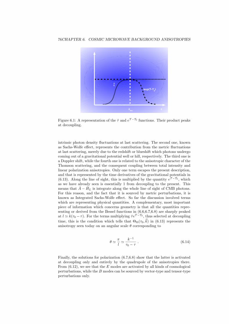
76CHAPTER 6. COSMIC MICROWAVE BACKGROUND ANISOTROPIES
Figure 6.1: A representation of the τ and eT −T0 functions. Their product peaksat decoupling.
intrinsic photon density fluctuations at last scattering. The second one, knownas Sachs-Wolfe effect, represents the contribution from the metric fluctuationsat last scattering, merely due to the redshift or blueshift which photons undergocoming out of a gravitational potential well or hill, respectively. The third one isa Doppler shift, while the fourth one is related to the anisotropic character of theThomson scattering, and the consequent coupling between total intensity andlinear polarization anisotropies. Only one term escapes the present description,and that is represented by the time derivatives of the gravitational potentials in(6.13). Along the line of sight, this is multiplied by the quantity eT −T0 , whichas we have already seen is essentially 1 from decoupling to the present. Thismeans that A− HL is integrate along the whole line of sight of CMB photons.For this reason, and the fact that it is sourced by metric perturbations, it isknown as Integrated Sachs-Wolfe effect. So far the discussion involved termswhich are representing physical quantities. A complementary, most importantpiece of information which concerns geometry is that all the quantities repre-senting or derived from the Bessel functions in (6.6,6.7,6.8) are sharply peakedat l ' k(τ0− τ). For the terms multiplying τ eT −T0 , thus selected at decoupling
time, this is the condition which tells that Θl0(τ0,~k) in (6.13) represents theanisotropy seen today on an angular scale θ corresponding to
θ ' π
l' k−1
τ0 − τ. (6.14)
Finally, the solutions for polarization (6.7,6.8) show that the latter is activatedat decoupling only and entirely by the quadrupole of the anisotropies there.From (6.12), we see that the E modes are activated by all kinds of cosmologicalperturbations, while the B modes can be sourced by vector-type and tensor-typeperturbations only.
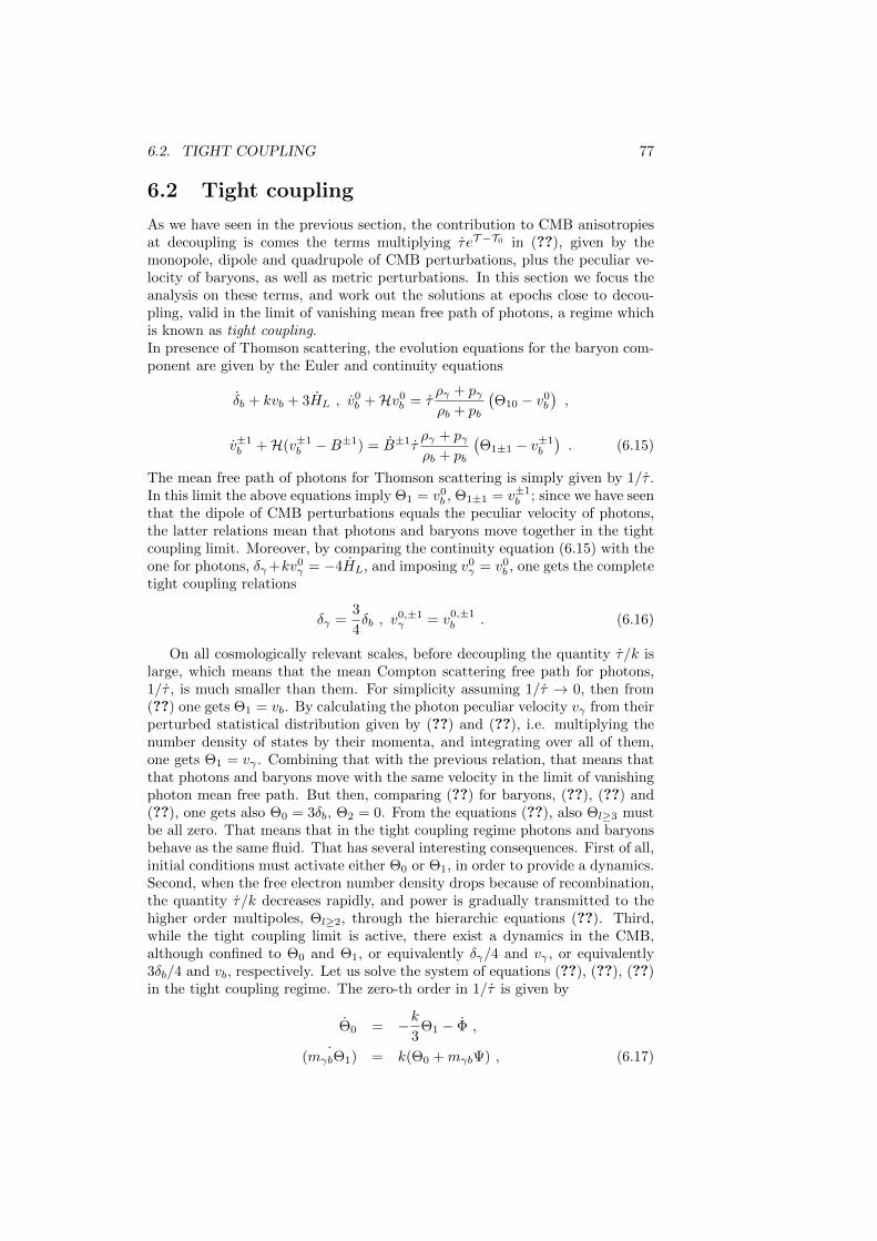
6.2. TIGHT COUPLING 77
6.2 Tight coupling
As we have seen in the previous section, the contribution to CMB anisotropiesat decoupling is comes the terms multiplying τ eT −T0 in (??), given by themonopole, dipole and quadrupole of CMB perturbations, plus the peculiar ve-locity of baryons, as well as metric perturbations. In this section we focus theanalysis on these terms, and work out the solutions at epochs close to decou-pling, valid in the limit of vanishing mean free path of photons, a regime whichis known as tight coupling.In presence of Thomson scattering, the evolution equations for the baryon com-ponent are given by the Euler and continuity equations
δb + kvb + 3HL , v0b +Hv0
b = τργ + pγρb + pb
(Θ10 − v0
b
),
v±1b +H(v±1
b −B±1) = B±1τ
ργ + pγρb + pb
(Θ1±1 − v±1
b
). (6.15)
The mean free path of photons for Thomson scattering is simply given by 1/τ .In this limit the above equations imply Θ1 = v0
b , Θ1±1 = v±1b ; since we have seen
that the dipole of CMB perturbations equals the peculiar velocity of photons,the latter relations mean that photons and baryons move together in the tightcoupling limit. Moreover, by comparing the continuity equation (6.15) with theone for photons, δγ+kv0
γ = −4HL, and imposing v0γ = v0
b , one gets the completetight coupling relations
δγ =3
4δb , v
0,±1γ = v0,±1
b . (6.16)
On all cosmologically relevant scales, before decoupling the quantity τ /k islarge, which means that the mean Compton scattering free path for photons,1/τ , is much smaller than them. For simplicity assuming 1/τ → 0, then from(??) one gets Θ1 = vb. By calculating the photon peculiar velocity vγ from theirperturbed statistical distribution given by (??) and (??), i.e. multiplying thenumber density of states by their momenta, and integrating over all of them,one gets Θ1 = vγ . Combining that with the previous relation, that means thatthat photons and baryons move with the same velocity in the limit of vanishingphoton mean free path. But then, comparing (??) for baryons, (??), (??) and(??), one gets also Θ0 = 3δb, Θ2 = 0. From the equations (??), also Θl≥3 mustbe all zero. That means that in the tight coupling regime photons and baryonsbehave as the same fluid. That has several interesting consequences. First of all,initial conditions must activate either Θ0 or Θ1, in order to provide a dynamics.Second, when the free electron number density drops because of recombination,the quantity τ /k decreases rapidly, and power is gradually transmitted to thehigher order multipoles, Θl≥2, through the hierarchic equations (??). Third,while the tight coupling limit is active, there exist a dynamics in the CMB,although confined to Θ0 and Θ1, or equivalently δγ/4 and vγ , or equivalently3δb/4 and vb, respectively. Let us solve the system of equations (??), (??), (??)in the tight coupling regime. The zero-th order in 1/τ is given by
Θ0 = −k3
Θ1 − Φ ,
˙(mγbΘ1) = k(Θ0 +mγbΨ) , (6.17)
78CHAPTER 6. COSMIC MICROWAVE BACKGROUND ANISOTROPIES
where mγb = 1+3ρb/4ργ . They combine in the following second order equationfor Θ:
˙(mγbΘ0) +k3
3Θ0 = −k
3
3mγbΨ− ˙(mγbΦ) . (6.18)
In absence of metric perturbations, the equation above has exact solutions:
Θ0 =1
m1/4γb
[A cos(ks) +B sin(ks)] , (6.19)
where A and B are constants, and
s =
∫ τ
0
dτ ′√3mγb
, (6.20)
represents the sound horizon for the fluid made by the tightly coupled baryonsand photons. Θ1 may be easily obtained from (6.17). The solution (6.19) may befurther simplified by neglecting the presence of baryons at decoupling. Indeed,at decoupling dark matter is about one order of magnitude more abundant thanradiation; baryons density is a few percent of the dark matter one and thereforeit makes sense to neglect them in order to clearify the phenomenology. In thislimit mγb = 1, s = τ/
√3, therefore
Θ0 = A cos
(kτ√
3
)+B sin
(kτ√
3
). (6.21)
The phenomenology does not change much if the metric fluctuations in the righthand side of equation (6.18) are taken into account. In the limit in which thegravitational potentials are constant in time, the solution (6.21) holds for Θ+Ψ,which means that the gravitational potential simply changes the zero level ofthe oscillations in (6.21).Let us now consider the evolution of the Θl≥3 coefficients in the tight couplingregime. As we have already seen, at the zero-th order in 1/τ they are simplyzero. The power transfers from Θ0 and Θ1 gradually to higher multipoles, withincreasing powers in k
τ . It is easy to see that an approximate solution for thatis given by
Θl = −kτ
0‖l−1
2l − 1Θl−1 , (6.22)
since in this way, Θl is always of order higher than Θl−1, and the terms involvingΘl and Θl+1 may be ignored in (??) because they are of order higher than Θl.
6.3 The CMB angular power spectrum
6.3.1 total intensity
We are now ready to compute the angular power spectrum of CMB anisotropesin the lab−frame. We start from the angular expansion of temperature anisotropy
Θ(τ, ~x, n) =∑lm
almYml , alm =
∫dΩYlm(n)Θ(τ, ~x, n) . (6.23)

6.3. THE CMB ANGULAR POWER SPECTRUM 79
Note that now the angular expansion is global and not depending on any Fourierwavevector, which does not even appear in (6.23). The coefficients of the angularpower spectrum are defined as
Cl =1
2l + 1
∑m
|alm|2 , (6.24)
and they correspond to the coefficients of the expansion of the correlation func-tion in Legendre polynomials:∫
dΩdΩ′[Θ(τ, ~x, n)Θ(τ, ~x, n′)]nn′=cos θ =∑l
(2l + 1)ClPl(cos θ) . (6.25)
The definitions above may be applied to any given sky signal. Usually the-ory predicts the average of the realizations of possible universes, with a givenvariance. For the angular power spectrum of the CMB, that means that the-ory predicts the average of the Cl over all possible realizations, which may bewritten as
Cl =< |alm|2 > , (6.26)
where the average is done over an assumed statistics.In our case
|alm|2 =
∫d3kd3k′dΩdΩ′
∑l′l′′
Y ml (n)Y m∗l (n′)Θl′(τ,~k)Gl′(~x,~knk)Θl′′(τ,~k′)∗Gl′′(~x,~k
′n′k)∗ .
(6.27)
The average in (6.26) operates in the product Θl′(τ,~k)Θl′(τ,~k′). The current
pictures of the early universe assume an initial Gaussianity in fluctuations. Thatmeans that the correlation between different wavevectors in null, and that thecoefficients depend on k only:
< Θl′(τ,~k)Θl′′(τ,~k′) >= δ(~k − ~k′)Θl′(τ, k)Θl′′(τ, k) > . (6.28)
This first eliminates one of the two Fourier integrals in (6.27). The angular com-
ponent of the harmonic functions Gl depends on n · k only, which is essentiallygiven by the Legendre polynomial Pl(n · k). A useful relation between Legendrepolynomials and spherical harmonics allows us to write
Pl′(n · k) =4π
2l + 1
∑m′
Y m′
l (n)Y m′∗
l (k) . (6.29)
and of course the same expression for Pl′′(n′ · k). This makes it possible to
perform the integral in n and n′ above, which selects l = l′ = l′′, m = m′ =m′′. Moreover, the fact that Θl(τ,~k) does not depend on the direction of the
wavevector makes the integrals of |Ylm(k)|2 over all the directions of ~k triviallyequal to 1. Working out the normalization factors, the result is
Cl =2
π
∫k2dk|Θl(τ, k)|2 , (6.30)
which makes explicit the connection between an observed quantity in the lab−frameon the left hand side with the angular expansion coefficients of the temperatureanisotropy on the right hand one, evaluated in the k−frame.
80CHAPTER 6. COSMIC MICROWAVE BACKGROUND ANISOTROPIES
6.3.2 polarization
6.4 Relation with cosmological observables
6.5 Status of CMB observation and future ex-pectations
6.6 excercises
6.6.1 question about cosmological distances for decoupling
Approximate the universe as completely radiation dominated from the Big Bangto time teq = 3 · 103 years, and completely matter dominated afterwards. Im-posing continuity for the scale factor a at equivalence, and neglecting the roleof baryons in the sound speed of the photon baryon fluid in the tight couplingregime, calculate the CMB sound horizon at decoupling, approximated as
rs =τdec√
3, (6.31)
where τ =∫ t
0dt/a(t) is the conformal time or comoving distance traveled by
a photon from the Big Bang to the time t; assume that decoupling occurs ata redshift tdec = 3 · 105 years. Evaluate the comoving distance from todayt0 = 15 · 109 years to the time of decoupling. Say qualitatively how such adistance is modified by the introduction of a cosmological constant which isrelevant in the recent cosmological expansion history.
6.6.2 question about angles and scales for the acousticpeaks
Evaluate the angles subtended in the sky by the acoustic peaks at decoupling inthe cosine and sine modes of the integral solution of CMB anisotropies, specifiedby
cos krs , sin krs . (6.32)
What is the difference in angle in the sky between the ones for the two modesoccurring at the largest angle in the sky? By using the approximate relationθ ' π/l linking the angle at which a given spherical harmonics or Legendre poly-nomials differs from zero to the actual multipole of the expansion, determine thelocations in l of the peaks for the two modes. Finally, determine the comovingwavenumbers and cosmological scales associated to these acoustic oscillations.
6.6.3 question about the CMB angular power spectrum
Consider the angular expansion of the CMB temperature perturbation in thek−frame:
Θ(τ0, ~x, n) =
∫d3k
(2π)3
∑lm
Θlm(τ0,~k)Glm(~k, ~x) . (6.33)
6.6. EXCERCISES 81
For flat cosmology the expansion set is given byGlm = (−i)l√
4π/(2l + 1)Ylm(nk)ei~k·~x.
Assume scalar-type perturbations only, setting m = 0. The angular expansionin the lab−frame is
alm =
∫dΩnΘ(τ0, ~x, n)Ylm(n) (6.34)
where Θ(τ0,~k, n) is given by (6.33). Show that
Cl =< |alm|2 >=
(4π
2l + 1
)2 ∫k2dk
2π2|Θl(τ0, k)|2 , (6.35)
exploiting the Gaussianity and isotropy assumption
< Θl0(τ,~k)Θl′0(τ,~k′) >= (2π)3δ(~k − ~k′)Θl(τ, k)Θ∗l′(τ, k) , (6.36)
and the relation
Yl0(n · k) =
√4π
2l + 1
∑m
Ylm(n)Y ∗lm(k) (6.37)
where the frame in which n and ~k are expressed is arbitrary, and may be chosento coincide with the lab−frame.
6.6.4 question about the role of baryons in acoustic oscil-lations
When baryons are considered, the equation for the monopole of CMB temper-ature perturbation is
˙(mbγΘ00) +k2
3Θ00 = −k
2
3mbγA− ˙(mbγHL) , (6.38)
where mbγ = 1 + 3ρb/4ργ . Assuming that the solution of the homogeneousequation may be written as
Θ00(τ,~k) = mpbγΘ00(0,~k) cos(ks) , (6.39)
where
s =
∫ τ
0
1√3mbγ
dτ ′ , (6.40)
determine p. Assuming a pure cosine solution, determine the ratio of the ampli-tudes of the n = 1 and n = 2 acoustic peaks occurring at ks = π and ks = 2π,respectively, as a function of ρb/ργ . Is this quantity increasing or decreasing ifρb/ργ is increased? Show that for fixed τ the peaks in the cosine and sine occurat larger wavenumbers with respect to the case in which ρb = 0. Note that thisdoes not imply that those oscillations are observed on smaller angular angles inthe CMB anisotropies, as if ρb/ργ is increased, the decoupling is also delayed.
82CHAPTER 6. COSMIC MICROWAVE BACKGROUND ANISOTROPIES
6.6.5 question about projection effects for CMB anisotropies
The monopole solution for CMB total intensity anisotropies, in flat cosmologies,Newtonian gauge, and Fourier space is given by
Θ00 +A = ΘA cos
(kτ√
3
)+ ΘI sin
(kτ√
3
)(6.41)
where A represents the gravitational potential and ΘA, ΘI are integration con-stants. Assume that the conformal time at decoupling (z = 1100) is aboutτdec = 200 Mpc comoving, and that decoupling itself is instantaneous. In the hy-pothesis that the Universe is matter dominated from decoupling to the present,calculate the angle subtended in the sky by the scales kn corresponding to thepeaks of the solution above, for the cosine (of course ignoring the n = 0 peak)and sine modes, separately. Assume that the Hubble constant today is H0 = 72km/s/Mpc. Discuss the effects of a non-zero Cosmological Constant, or non-zero curvature on those angles, saying if they get bigger or smaller with respectto a matter dominated Universe, and in which cases.
6.6.6 question about an integral solution to CMB anisotropies
The Boltzmann equation for the temperature CMB perturbations Θ(η, ~x, n) inthe Fourier space is
Θ + ik cos θΘ + Φ + ik cos θΨ = τ(Θ0 −Θ− i cos θve) , (6.42)
where η is the conformal time, k = |~k| is the Fourier wavevector amplitude, θis the angle between the photon propagation direction n and the wavevector, Φand Ψ are the scalar-type perturbations to the metric in the Newtonian gauge,Θ0 =
∫dnΘ is the monopole of the CMB temperature perturbations, ve = |~ve|
is the amplitude of the electron peculiar the metric, τ = aneσT is the differentialThomson optical depth as a function of the scale factor a, the electron numberdensity ne and the Thomson cross section σT .Verify that the above equation is equivalent to
d
dη[Θ exp (ikη cos θ + τ)] =
= [−Φ− ik cos θΨ + τ(Θ0 − i cos θve)] exp (ikη cos θ + τ) . (6.43)
where τ =∫ η
0τ dη. Integrating the equation above between η = 0 and the
present, η = η0, obtain the solution for Θ expressed as an integral in the con-formal time plus a quantity containing the initial condition, Θ(0). By writing
τ =
∫ η
0
τ dη =
∫ η0
0
τ dη −∫ η0
η
τ dη = τ0 − τtod(η) , (6.44)
where the last equality defines the Thomson scattering optical depth τtod(η),show that the initial condition in the solution above is suppressed by a factorexp (−τ0) with respect to the integral part.Thus, neglecting the initial condition on Θ, focus on the integral solution. Itcan be divided in a block of terms proportional to exp (−τtod), and another oneproportional to τ exp (−τtod). By using the expression τ = aneσT , and knowing

6.6. EXCERCISES 83
that the electron density is different from zero at early times and abrubtly shutsoff at decoupling, 1 + zdec = 1/adec ' 1100, show qualitatively that the firstblock of terms defined above contributes to the CMB perturbations up to thepresent, while the second one is active at decopuling only, being negligible beforeand after that epoch.Perform the expansion of Θ in spherical harmonics, obtaining an expression for
Θl =
∫dnΘY 0
l (n) , (6.45)
by using the k−frame, in which ~k is the polar axis, and the known expansion
exp (i~k · ~r) =∑l
(−i)l√
4π(2l + 1)jl(kr)Y0l (r) , (6.46)
with ~r = (η − η0)n.
6.6.7 question about Silk damping
The solution (6.41) presents an infinite series of peaks, in time or alternativelyin wavenumbers, with constant amplitude. On the other hand, we know thatCMB anisotropies vanish on angular scales smaller than about 10 arcminutes.By considering the integral solution to the Boltzmann equation, for scalar per-turbations only, no Doppler, polarization or integrated effects,
Θl0 = (2l + 1)
∫ τ0
0
dτ(Θ00 +A)τ e−∫ τ0τ
τoddτ′jl[k(τ0 − τ)] , (6.47)
where τod is the differential optical depth, give a physical reason of such damp-ing. Use the fact that the anisotropy starts vanishing at 10 arcminute scale inorder to make your answer more quantitative and get an rough estimate of theduration of the decoupling process.

84CHAPTER 6. COSMIC MICROWAVE BACKGROUND ANISOTROPIES
Bibliography
Bardeen, 1980, ...
...
Komatsu E., et al., 2009, Astrophys. J. Supp. 180, 330
85