Linear Analysis

Lectured by B. J. Green (and B. Schlein)

Michaelmas Term 2010 (and 2008)

1 Normed Spaces 1

2 The Hahn-Banach Theorem 11

3 The Baire Category Theorem 16

4 The Space C(X) 23

5 Weak Topologies on Normed Spaces 33

6 Hilbert Space 39

7 Spectral Theory 48

Hahn-Banach handout (2011)Examples Sheets

These notes combine the material lectured in 2008 and 2010.

Chapters 1, 3, 4, 6, 7 were lectured in 2010.

Chapters 2, 5 were lectured in 2008.

Last updated: Wed 29th May, 2019

These have not really been proof-read yet, and typing up analysis

is prone to mistakes. So please do let me know of any corrections:

glt1000@cam.ac.uk

LINEAR ANALYSIS (D) 24 lectures, Michaelmas term

Part IB Linear Algebra, Analysis II and Metric and Topological Spaces are essential.

Normed and Banach spaces. Linear mappings, continuity, boundedness, and norms. Finite-dimensional normed spaces. [4]

The Baire category theorem. The principle of uniform boundedness, the closed graph theoremand the inversion theorem; other applications. [5]

The normality of compact Hausdorff spaces. Urysohn’s lemma and Tiezte’s extension the-orem. Spaces of continuous functions. The Stone-Weierstrass theorem and applications.Equicontinuity: the Ascoli-Arzela theorem. [5]

Inner product spaces and Hilbert spaces; examples and elementary properties. Orthonormalsystems, and the orthogonalization process. Bessel’s inequality, the Parseval equation, andthe Riesz-Fischer theorem. Duality; the self duality of Hilbert space. [5]

Bounded linear operations, invariant subspaces, eigenvectors; the spectrum and resolvent set.Compact operators on Hilbert space; discreteness of spectrum. Spectral theorem for compactHermitian operators. [5]

Appropriate books

B. Bollobas Linear Analysis. 2nd Edition, Cambridge University Press 1999 (£22.99 paper-back).C. Goffman and G. Pedrick A First Course in Functional Analysis. 2nd Edition, OxfordUniversity Press 1999 (£21.00 Hardback)W. Rudin Real and Complex Analysis. McGraw-Hill International Editions: MathematicsSeries (£31.00 Paperback)

1. Normed Spaces

In this course all vector spaces V will be over R or C. Usually it doesn’t matter which. Theywon’t always (or even usually) be finite dimensional. Our vector spaces will have additionalanalytic structure; this makes the theory much more interesting.

By a norm on V we mean a map ‖ ‖ : V → R>0 satisfying the following:

(i) ‖x‖ = 0 ⇐⇒ x = 0

(ii) ‖λx‖ = |λ| ‖x‖ for all λ ∈ R or C

(iii) ‖x+ y‖ 6 ‖x‖+ ‖y‖ (‘subadditive’)

Think of ‖x‖ as the ‘length’ of x, but don’t rely on geometric intuition too much!

Examples

1. V = R, and ‖x‖ = |x| is absolute value.

2. V = Rn, with the Euclidean norm: ‖x‖2 =√|x1|2 + . . .+ |xn|2, where x = (x1, . . ., xn).

Or with the ℓ1-norm: ‖x‖1 = |x1|+ . . .+ |xn|Or with the ℓ∞-norm: ‖x‖∞ = max

i=1,...,n|xi|

3. S = any set, V = B(S) = vector space of bounded real-valued functions on S.

‘sup norm’: ‖f‖∞ = sups∈S

|f(s)|

4. V = C[0, 1] = continuous functions on [0, 1].

Possible norm: ‖f‖∞ = supt∈[0,1]

|f(t)|. (Actually max since f attains its bounds.)

Also works in any metric (topological) space X in place of C[0, 1].

‖f‖1 =∫ 1

0 |f(t)| dt‖f‖2 =

(∫ 1

0|f(t)|2 dt

)1/2

proof that these are norms – exercise

5. V = Ck[a, b] = space of k-times continuously differentiable functions on [a, b].

‖f‖ = supt∈[a,b]

(|f(t)|+ |f ′(t)|+ . . .+ |fk(t)|

)

6. V = Riemann-integrable integrable functions on [0, 1].

‖f‖1 =∫ 1

0 |f(t)| dt – only a seminorm, since one can have ‖f‖1 = 0 with f 6= 0.

E.g., f(x) =

{0 x ∈ (0, 1]1 x = 0

.

Make it a normed space by quotienting these out: f ∼ g if∫ 1

0 |f(t)− g(t)| dt = 0.

7. ℓ1 = {(x1, x2, . . .) :∑∞

i=1 |xi| <∞}ℓ2 = {(x1, x2, . . .) :

∑∞i=1 |xi|2 <∞} – Hilbert space

ℓ∞ = {(x1, x2, . . .) : supi |xi| <∞}8. ℓp-spaces. Let 1 6 p <∞, V = Rn.

‖x‖p = (∑n

i=1 |xi|p)1/p

– this is called ℓnp . (Proof of triangle inequality: see below.)

ℓp = {(x1, x2, x3, . . .) :∑∞

i=1 |xi|p <∞} with ‖x‖p = (∑∞

i=1 |xi|p)1/p

.

This generalises example 7.

1

ℓp-norms, Holder’s Inequality and Minkowski’s Inequality

Holder’s Inequality. Suppose 1 < p < ∞. Define the conjugate index q by 1p + 1

q = 1.

Let (ai)ni=1 and (bi)

ni=1 be two sequences of complex numbers. Then

n∑

i=1

|aibi| 6( n∑

i=1

|ai|p)1/p( n∑

i=1

|bi|q)1/q

.

Remarks. Fancier statement is that |〈x, y〉| 6 ‖x‖p‖y‖q if x, y ∈ Cn.

In the special case p = q = 2, one recovers Cauchy-Schwarz.

The fancier statement is also true and easy with p = 1, q = ∞. By convention, p = 1and q = ∞ are thought of as conjugate indices: ‘ 11 + 1

∞ = 1’.

We first need to prove:

The weighted AM-GM inequality. If a1, . . ., an > 0, and if λ1, . . ., λn ∈ [0, 1] satisfyλ1 + . . .+ λn = 1, then

aλ1

1 . . .aλnn 6 λ1a1 + . . .+ λnan.

This is a generalisation of the usual AM-GM, which is the case λi = 1/n.

Proof. We use the concavity of the function f(x) = log x, which follows from the fact thatf ′′(x) = −1/x2 6 0. (Exercise: this really implies concavity.)

We have f(λ1x1 + . . .+ λnxn) > λ1f(x1) + . . .+ λnf(xn) – Jensen’s Inequality.

In the specific case of f(x) = log x we get

λ1 log x1 + . . .+ λn log xn 6 log(λ1x1 + . . .+ λnxn).

Exponentiating both sides gives weighted AM > GM. 2

A particular example of this (in the case n = 2) is that ab 6ap

p+bq

q(∗), whenever

a, b ∈ [0,∞) and p, q are conjugate indices.

Proof of Holder’s Inequality. The inequality is homogeneous in the sense that if it is truefor ai, bi, then it is also true for λai and µbi for any λ, µ ∈ R \ {0}.

The inequality is manifestly true when either∑ |ai|p or

∑ |bi|q equals 0 (since theneither all ai or all bi are 0). Otherwise, by an appropriate choice of λ, µ we may assumethat

∑ni=1 |ai|p =

∑ni=1 |bi|q = 1.

But under these conditions, by (∗) we do indeed have∑n

i=1 |aibi| 6 1p

∑ni=1 |ai|p +

1q

∑ni=1 |bi|q = 1. 2

Minkowski’s Inequality. Suppose ai, bi ∈ C and that 1 < p <∞. Then

( n∑

i=1

|ai + bi|p)1/p

6

( n∑

i=1

|ai|p)1/p

+

( n∑

i=1

|bi|p)1/p

.

2

In other words, the ℓp-norm on Rn (or Cn) is indeed a norm, since we have the triangleinequality.

Proof.

n∑

i=1

|ai + bi|p =

n∑

i=1

|ai + bi|p−1|ai + bi| 6

n∑

i=1

|ai + bi|p−1|ai|+n∑

i=1

|ai + bi|p−1|bi|.

By Holder, this is at most

( n∑

i=1

|ai + bi|(p−1)q

)1/q( n∑

i=1

|ai|p)1/p

+

( n∑

i=1

|ai + bi|(p−1)q

)1/q( n∑

i=1

|bi|p)1/p

Now, (p− 1)q = p, since 1p + 1

q = 1. Therefore this is

( n∑

i=1

|ai + bi|p)1/q

(( n∑

i=1

|ai|p)1/p

+

( n∑

i=1

|bi|p)1/p

)

Divide though by(∑ |ai + bi|p

)1/q.

( n∑

i=1

|ai + bi|p)1− 1

q

6

( n∑

i=1

|ai|p)1/p

+

( n∑

i=1

|bi|p)1/p

.

But 1− 1q = 1

p , so done. 2

Banach Spaces

If V is a normed space with norm ‖ ‖ then it can be regarded as a metric space by definingd(x, y) = ‖x− y‖. (Easy exercise to see that this is a metric space.)

Definition. V is a Banach space if it is complete with respect to this metric. (I.e., Cauchysequences converge.)

Examples

• R is a Banach space.

• Rn with ℓ1-norm: ‖x‖1 = |x1|+ . . .+ |xn|.The metric induced on Rn is exactly the product metric on Rn, viewed as a product ofn copies of R.

Recall from Met&Top that if X,Y are metric spaces then we can define a metric onX × Y by d

((x1, y1), (x2, y2)

)= dX(x1, x2) + dY (y1, y2).

If X and Y are complete then so is X×Y . (Proof: exercise.) If((xn, yn)

)∞n=1

is Cauchyin X × Y then (needs justifying) (xn) is Cauchy in X and (yn) is Cauchy in Y . Letxn → x∗, yn → y∗, then (xn, yn) → (x∗, y∗).

Proposition. ‘Any two norms on a finite-dimensional space are equivalent.’

Suppose ‖ ‖ and ‖ ‖′ are two norms on Rn (or Cn). Then they are equivalent in thesense that there are c1, c2 > 0 such that c1‖x‖ 6 ‖x‖′ 6 c2‖x‖ for all x ∈ V .

(Exercise: this defines an equivalence relation.)

Proof. Since ‘equivalence’ is indeed an equivalence relation, it suffices to show that a givennorm ‖ ‖ is equivalent to the ℓ1-norm, ‖ ‖1.

3

We claim that x 7→ ‖x‖ is continuous in the metric induced by the ℓ1-norm. To seethis, suppose that ‖v − w‖1 6 δ, that is to say

∑ni=1 |vi − wi| 6 δ. Then

‖v − w‖ =

∣∣∣∣∣∣∣∣

n∑

i=1

(vi − wi)ei

∣∣∣∣∣∣∣∣ with e1, . . ., en the standard basis

6

n∑

i=1

|vi − wi| ‖ei‖ using scalar multn and triangle ineq. for ‖ ‖

6 M

n∑

i=1

|vi − wi| where M = supi

‖ei‖

6 Mδ

So if ‖v−w‖1 6 δ then ‖v−w‖ 6Mδ. By the triangle inequality,∣∣‖v‖−‖w‖

∣∣ 6 ‖v−w‖.So, in the ε-δ definition of continuity, we may take δ = ε/M . This establishes the claim.

Now, the unit sphere {x : ‖x‖1 = 1} ⊂ Rn is closed and bounded, hence compact. Sothe function x 7→ ‖x‖, being continuous, is bounded and attains its bounds.

In particular, inf‖x‖1=1

‖x‖ = min‖x‖1=1

‖x‖ 6= 0, since the only vector with norm zero is 0.

So there are c1, c2 > 0 such that c1 6 ‖x‖ 6 c2 for all x with ‖x‖1 = 1. This impliesc1‖x‖1 6 ‖v‖ 6 c2‖v‖1, for all v (take x = v/‖v‖1). 2

Corollary. Any finite-dimensional normed space is a Banach space.

Proof. Equivalent norms give rise to equivalent metrics: c1d1(x, y) 6 d2(x, y) 6 c2d1(x, y).And Cauchy sequences and convergence in one metric means the same as in the other.(Exercise: check details.)

Norms and convex bodies

There is a correspondence between norms on Rn and closed, bounded, centrally symmetric(i.e. x ∈ K ⇔ −x ∈ K) convex bodies K containing a ball Bε(0) about the origin.

For (⇒), it is easy to show that the triangle inequality for ‖ ‖ implies that {x : ‖x‖ 6 1} isa convex body.

For (⇐), suppose K is such a convex body. We can define ‖x‖ to be the dilation factor of Krequired to ‘hit‘ x, that is ‖x‖ = min

λ{x ∈ λK}.

Why is it a norm? First check it’s well-defined (using non-empty interior). The triangleinequality follows since λK + µK ⊂ (λ + µ)K – a consequence of convexity.

ℓ∞ ℓ2

✫✪✬✩

��

❅❅

❅❅

��

ℓ1

4

Back to examples of Banach spaces

• C[0, 1] = continuous functions on [0, 1] with ‖f‖ = ‖f‖∞ = supt |f(t)| is a Banachspace The completeness follows as a consequence of the fact that a uniformly convergentsequence (fn)

∞n=1 of continuous functions converges to a continuous function f . (See

Analysis II.)

Note. (fn)∞n=1 being uniformly convergent is the same thing as (fn)

∞n=1 being a Cauchy

sequence in ‖ ‖ (or rather, in the metric space induced by this norm).

• L1 = C[0, 1] = continuous functions on [0, 1], with ‖f‖ = ‖f‖1 =∫ 1

0 |f(t)| dt. This isnot a Banach space. We can have a Cauchy sequence of functions fn:

❅❅12

1

❆❆12

1

‘−→’

12

1

E.g., fn(x) =

0 if x >12 + 1

n

1 if x 612 − 1

n12 − n

2 (x− 12 ) if 1

2 − 1n 6 x 6 1

2 + 1n

This is Cauchy in L1, since ‖fm − fn‖ 6 max(

2m ,

2n

)→ 0 as m,n→ ∞.

However, fn does not converge to any continuous function f . What would f(12

)be?

Wlog, f(12

)6 1

2 . Since f is continuous, f(x) 6 34 for

∣∣x− 12

∣∣ 6 δ, for some δ.

By contrast, fn(x) = 1 if 12 − δ 6 x 6

12 − δ

2 for n sufficiently large.

Hence, if n is big enough, ‖f − fn‖1 >14

δ2 = δ

8 . So fn 6→ f in L1.

Exercise. On C[0, 1], the norms ‖ ‖∞ and ‖ ‖1 are inequivalent. (Easy.)

Remark. For essentially the same reason, C[0, 1] is not a Banach space in any Lp-norm,1 6 p 6 ∞.

More examples

• ℓp = {(x1, x2, x3, . . .) ∈ CN :∑∞

i=1 |xi|p <∞}, with the ℓp-norm, ‖x‖p = (∑ |xi|p)1/p.

(This is a norm by Minkowski’s inequality – let n→ ∞.)

This is complete and hence a Banach space.

Proof. Let (xn)∞n=1 be a Cauchy sequence in ℓp. Each xn is a sequence; write them as

x1 = (x11, x12, x13, . . .), x2 = (x21, x22, x23, . . .), . . .

We must prove that there exists x∗ ∈ ℓp such that ‖xn − x∗‖p → 0.

Observe that for any fixed i, |xni − xmi| 6 ‖xn − xm‖p, and therefore (xni)∞n=1 is

a Cauchy sequence. Since C is complete, there exists x∗i such that xni → x∗i .

Define x∗ = (x∗1, x∗2, . . .). Claim that xn → x∗ in ℓp.

Claim. Let m be such that ‖xm−xn‖p 6 ε for all n > m. Then ‖xm−x∗‖p 6 ε.

Then we can conclude that ‖xm−x∗‖p → 0. And x∗ ∈ ℓp, since ‖x∗‖p 6 ‖xm‖p+‖x∗ − xm‖p 6 ‖xm0

‖p + 1 (if m0 is large enough) <∞.

It remains to prove the claim.

5

Proof of claim. Suppose ‖xm − xn‖p 6 ε for all n > m. Let R be arbitrary.

Then∑R

i=1 |xmi − xni|p 6 εp. Let n→ ∞, we get∑R

i=1 |xmi − x∗i |p 6 εp.

Let R → ∞, we get∑∞

i=1 |xmi − x∗i |p 6 εp.

That is ‖xm − x∗‖p 6 ε, as required. 2

Note. In particular, ℓ2 = Hilbert space is complete.

Completion of Normed Spaces

This section is from the 2008 notes.

Let (V, ‖ ‖) be a normed space. The construction of the completion of V is as follows. LetCV be the set of all Cauchy sequences in V . This is a vector space: if x = (xn) and y = (yn),then λx+ µy = (λxn + µyn).

Let NV = {(xn) : xn → 0} be the subset of CV consisting of null sequences. This is in fact asubspace of CV , and so V = CV /NV is a vector space.

We define a norm on V . For x ∈ CV , let p(x) = limn→∞ ‖xn‖, which is well-defined as ‖xn‖is Cauchy in R. We have

(i) p(x) = 0 iff x ∈ NV

(ii) p(λx) = |λ| p(x)(iii) p(x+ y) 6 p(x) + p(y) for all x, y ∈ CV .

and p induces p on V , by p : V → R+, [x] 7→ p(x).

This is well-defined, as x ∼ y ⇒ x − y ∈ NV ⇒ xn − yn → 0 ⇒ ‖xn‖ − ‖yn‖ → 0 ⇒limn→∞ ‖xn‖ = limn→∞ ‖yn‖ ⇒ p(x) = p(y).

And p is a norm on V as p([x]) = 0 ⇔ p(x) = 0 ⇔ x ∈ NV ⇔ [x] = 0.

So (V , p) is a normed space.

We can regard (V, ‖ ‖) as a dense subset of (V , p). Define ϕ : V → V , x 7→ [(x, x, . . .)]. Thenϕ is linear and p(ϕ(x)) = ‖x‖, so ϕ is isometric, and in particular injective.

Claim. ϕ(V ) = V , where ϕ(V ) is the closure of ϕ(V ) in V .

Proof. Let [x] ∈ V and ε > 0. Then x = (xn) is Cauchy, so ‖xm − xn‖ 6 ε for m,n > n0.Then p

(ϕ(xn0

)− [x])= p(xn0

− x1, xn0− x2, . . .) 6 ε. 2

If V is complete then V ∼= V , with ϕ(V ) = V . For if [x] ∈ V , write x = (xn) ∈ CV andx∞ = limn→∞ xn. Then x∞ ∈ V by the completeness of V we have ϕ(x∞) = [x].

Claim. (V , p) is always complete.

Proof. Let ([xn]) be a Cauchy sequence in V , so that (xn) is Cauchy in V for all n. Sinceϕ(V ) = V , there exists zn ∈ V such that p(ϕ(zn)− [xn]) 6 1

2n , for each n ∈ N.

6

‖zn − zm‖ = p(ϕ(zn)− ϕ(zm)

)

6 p(ϕ(zn)− [xn]

)+ p([xn]− [xm]

)+ p([xm]− ϕ(zm)

)

61

2n+ p([xn]− [xm]

)+

1

2m→ 0 as n,m→ ∞

So z = (zn) is Cauchy in V .

p([z]− [xn]

)= lim

m→∞‖zm − xnm‖

6 lim supm→∞

‖zm − zn‖+ lim supm→∞

‖zn − xnm‖

61

2n→ 0 as n→ ∞

So [xn] → [z] as n→ ∞ and thus (V , p) is complete. 2

Definition. Let V be a normed space. A completion of V is a triple (V , p, ϕ) such that(V , p) is a complete normed space, and ϕ : V → V is linear, isometric, and ϕ(V ) = V .

Theorem. The completion of a normed space V exists and is uniquely determined up to anisometric isomorphism.

Proof. Exercise.

Proposition. A normed space V is complete iff every absolutely convergent series converges.

Proof. Suppose V is complete and∑∞

n=1 ‖xn‖ <∞. Then forM > N , we have∥∥∑M

n=N xn∥∥

6∑M

n=N ‖xn‖ → 0, as N → ∞. So the series is Cauchy, hence converges.

Conversely, suppose that every absolutely convergent series is convergent, and let (xn)be a Cauchy sequence. It is sufficient to show that there exists subsequence xni

con-verges to some x ∈ V , as then: ‖xm − x‖ 6 ‖xm − xni

‖+ ‖xni− x‖ → 0 as m, i→ ∞.

To prove there is a convergent subsequence, choose n1 ∈ N such that ‖xn1− xm‖ 6

12

for all m > n1. Then choose n2 > n1 such that ‖xn2− xm‖ 6 1

22 for all m > n2. Andso on. Then xnk+1

= xn1+ (xn2

− xn1) + . . .+ (xnk+1

− xnk).

But∑∞

i=1 ‖xni+1− xni

‖ 6∑∞

i=112i = 1. So xni

→ x, for some x ∈ V . 2

Linear operators

Let X,Y be two normed spaces. A linear map T : X → Y is said to be continuous if T isa continuous map in the metric spaces induced by the norms on X and Y .

That is, T must be continuous at every point x0 ∈ X , which means that for all ε > 0 thereexists δ > 0 such that ‖x− x0‖X 6 δ implies ‖Tx− Tx0‖Y 6 ε.

Lemma. Let T : X → Y be a linear map between normed spaces. The following areequivalent.

(1) T is continuous

(2) T is continuous at some x0

(3) T is bounded, meaning that T (BX(1)) ⊂ BY (R) for some R (where BX(r) ={x ∈ X : ‖x‖ < r}). Equivalently, ‖Tx‖Y 6 R‖x‖X .

7

As a result of this we always speak of bounded operators and never continuous ones.

Proof. (1) ⇒ (2). Trivial.

(2) ⇒ (3). If T is continuous at x0 then there exists δ > 0 such that ‖x − x0‖X < δimplies ‖Tx− Tx0‖Y 6 1. I.e., ‖T (x− x0)‖ 6 1, by linearity of T .

Hence T (BX(δ)) ⊂ BY (1). By linearity of T again, this implies T (BX(1)) ⊂ BY (1/δ).

(3) ⇒ (1). Note (3) implies that ‖Tx‖Y 6 R‖x‖X . Hence if ε > 0, take δ = ε/R. Thenif ‖x− x0‖ 6 δ we have ‖Tx− Tx0‖Y = ‖T (x− x0)‖Y 6 R‖x− x0‖X 6 ε.

So T is continuous at x0. 2

The infimum of all possible values of R for which ‖Tx‖Y 6 R‖x‖X is called the operatornorm of T , written ‖T ‖. Equivalently, ‖T ‖ = sup

‖x‖X=1

‖Tx‖Y .

Examples

1. Linear maps between finite-dimensional spaces. These are always bounded.

Indeed, suppose X = Rm, Y = Rn, and that T : X → Y is given by a matrix A = (aij).

Let x =∑

j λjej , then Tx =∑

j λjTej =∑

j λj (∑

i aijei) =∑

i(∑

j λjaij)ei. Hence

‖Tx‖∞ = maxi |∑

j λjaij | 6 maxi∑

j |λjaij | 6 maxj |λj | ·maxi∑

j |aij | = ‖x‖∞ ·M ,

where M = maxi∑

j |aij |, since ‖x‖∞ = maxj |λj |.

Since any two norms on Rn are equivalent, T is bounded by any norm.

More simply. Let M = maxi ‖Tei‖∞. Then T is bounded as a map ℓm1 → ℓn∞, since

‖Tx‖∞ = ‖∑j λjTej‖∞ 6∑

j |λj | ‖Tej‖∞ 6M(∑

j |λj |) =M‖x‖1.

So done since any two norms on a finite-dimensional vector space are equivalent.

2. Shift map. Let X = ℓ1 = {(x1, x2, . . .) :∑ |xi| <∞}.

Define T : X → X by T (x1, x2, . . .) = (0, x1, x2, . . .),S : X → X by S(x1, x2, . . .) = (x2, x3, . . .).

Both are linear and ‖S‖ = ‖T ‖ = 1. Note that S ◦T = id, T ◦ S 6= id. (So existence ofa left inverse does not imply existence of a right inverse.)

3. Suppose X = C(1)[0, 1], the continuously differentiable functions on [0, 1]. We previ-ously mentioned the norm ‖f‖ = supt

(|f(t)|+ |f ′(t)|

).

We also have the sup norm, ‖f‖∞ = supt |f(t)|. Let Y = C[0, 1] with the sup norm,and define T : X → Y by T (f) = f ′. This is certainly linear.

T is bounded if X is given the first norm, but not if X has the sup norm. (Take abounded function with unbounded derivative.)

8

Suppose X,Y are normed spaces. We write B(X,Y ) = {T : X → Y : ‖T ‖ <∞}.

When Y = R (or C) we write X∗ = B(X,R) (or B(X,C)). This is the dual space of X .Elements of X∗ are called functionals.

B(X,Y ) is a vector space and in fact a normed space with the operator norm:

• If S, T ∈ B(X,Y ) we define (S + T )(x) = Sx+ Tx.

Then sup‖x‖=1

‖(S + T )(x)‖ 6 sup‖x‖=1

‖Sx‖+ sup‖x‖=1

‖Tx‖ = ‖S‖+ ‖T ‖.

• Same with scalar multiplication: (λT )(x) = λTx. Exercise: ‖λT ‖ = |λ| ‖T ‖.

The following is the most important fact about B(X,Y ).

Lemma. If Y is a Banach space (i.e. Y is complete) then so is B(X,Y ).

In particular, X∗ is a Banach space for every X .

Proof. Suppose that (Tn)∞n=1 is a Cauchy sequence in B(X,Y ), i.e. ‖Tm − Tn‖ → 0 as

m,n→ ∞. We need to find T ∈ B(X,Y ) such that Tn → T in the operator norm.

Let x ∈ X . The sequence (Tnx)∞n=1 is Cauchy, because ‖Tmx−Tnx‖Y 6 ‖Tm−Tn‖ ‖x‖,

which → 0 as m,n→ ∞. But Y is a Banach space and so Tnx→ x∗.

Define Tx = x∗. It’s easy to check that T is linear: Tn(x+ y) = Tnx+ Tny → x∗ + y∗,so (x+ y)∗ = x∗ + y∗.

Also, Tn → T in the operator norm, as follows.

Let ε > 0 and suppose ‖Tm − Tn‖ 6 ε for all n > m. Then ‖Tmx − Tnx‖Y 6 ε‖x‖X .Letting n→ ∞, we get ‖Tmx−Tx‖Y 6 ε‖x‖X . For such an m, we have ‖Tm−T ‖ 6 ε.Hence Tm → T in the operator norm.

Note ‖T ‖ is bounded, since ‖T ‖ 6 ‖Tn‖+ ‖T − Tn‖ 6 ‖Tn‖+ 1 for a suitable n. 2

(Compare the proof that ℓp is complete.)

Lemma. Suppose 1 < p <∞. Let 1p + 1

q = 1. Then ℓ∗p∼= ℓq (‘isometrically isomorphic’).

Notes. 1. (X, ‖ ‖X) and (Y, ‖ ‖Y ) are isometrically isomorphic if there is a linearisomorphism θ : X → Y such that ‖θx‖Y = ‖x‖X .

2. This gives us ‘another’ proof that ℓp is complete.

Proof. Let e1 = (1, 0, 0, . . .), e2 = (0, 1, 0, . . .), e3 = (0, 0, 1, 0, . . .), . . . in ℓp. (Exercise: thisis not a basis for ℓp as a vector space.)

Suppose that ϕ ∈ ℓ∗p. Let ϕ(ei) = yi.

Clearly ϕ((x1, . . ., xn, 0, 0, . . .)

)= ϕ(x1e1 + . . .+ xnen) = x1y1 + . . .+ xnyn.

However, if x = (x1, x2, . . .) ∈ ℓp then we have (x1, . . ., xn, 0, 0, . . .) → x in ℓp, because

‖x− (x1, . . ., xn, 0, 0, . . .)‖p =(∑

i>n |xi|p)1/p → 0. (Note: this is false in ℓ∞.)

9

It follows that ϕ(x) = ϕ((x1, x2, . . .)

)=∑∞

i=1 xiyi = limn→∞ ϕ((x1, . . ., xn, 0, 0, . . .)

).

However, the yi are not arbitrary.

Claim. ϕ ∈ ℓ∗p ⇐⇒ (y1, y2, . . .) ∈ ℓq. (This provides the isomorphism ℓ∗p∼= ℓq.)

Proof of claim. (⇐) is an immediate consequence of Holder’s inequality. Indeed, if(y1, y2, . . .) ∈ ℓq then |ϕ(x)| = |∑xiyi| 6 ‖x‖p‖y‖q.

So ϕ is a bounded linear functional with ‖ϕ‖ 6 ‖y‖q. (In fact, equality occurs.)

(⇒). Suppose conversely that∣∣∑∞

i=1 xiyi∣∣ 6M

(∑∞i=1 |xi|p

)1/pfor all (xi) ∈ ℓp.

Let xi =

{|yi|qy−1

i if i 6 N0 if i > N

, for fixed N .

Then (xi) ∈ ℓp, and so∑N

i=1 |yi|q 6M(∑N

i=1 |yi|(q−1)p)1/p

.

Hence, since (q − 1)p = q and 1/p = 1− 1/q, we have(∑N

i=1 |yi|q)1/q

6M .

But N was arbitrary, so we are done. 2

Corollary. ℓp is complete for 1 < p <∞.

Proof. ℓp = ℓ∗q and every dual space is complete. 2

Note. Note. This doesn’t work for ℓ1, because ℓ1 is much smaller than ℓ∗∞. (In fact, ℓ∞ isa pretty exotic object.)

ℓ∞ is the dual of ℓ1. However, ℓ1 is the dual of c0, the space of bounded sequences(x1, x2, . . .) with xi → 0 as i → ∞. The proof is the same as for the above norm,because the ‘convergence of the approximations’ now holds.

Adjoints

Suppose X,Y are normed spaces and T ∈ B(X,Y ).

Define the adjoint map T ∗ : Y ∗ → X∗ by (T ∗g)(x) = g(Tx) for all g ∈ Y ∗, x ∈ X .

Easy to show T ∗ is linear and bounded. Indeed: ‖T ∗g(x)‖ = ‖g(Tx)‖ 6 ‖g‖ ‖Tx‖ 6

‖g‖ ‖T ‖ ‖x‖, all g ∈ Y ∗, x ∈ X .

Therefore, ‖T ∗g‖ 6 ‖g‖ ‖T ‖, and therefore ‖T ∗‖ 6 ‖T ‖.

(In fact, equality occurs: requires the Hahn-Banach theorem.)

10

2. The Hahn-Banach Theorem

Throughout this section, X∗ is always a Banach space. But could X∗ = {0}?

Definition. Let X be a real vector space. A function p : X → R is said be a convexfunctional if:

(i) p(αx) = αp(x) for all α > 0, x ∈ X

(ii) p(tx+ (1− t)y) 6 tp(x) + (1 − t)p(y) for all t ∈ [0, 1], and all x, y ∈ X .

Note convexity follows from subadditivity, p(x+ y) 6 p(x) + p(y), and positive homogeneity.

Lemma. Let X be a real vector space, p : X → R a convex functional on X , M ⊂ X alinear subspace, and f :M → R a linear functional on M such that f(x) 6 p(x) for allx ∈M . Let x0 ∈ X \M and write M ′ =M + 〈x0〉.

Then there exists F :M ′ → R such that F |M = f , and F (x) 6 p(x) for all x ∈M ′

Proof. Any z ∈ M ′ can be written as z = y + tx0, with y ∈ M , t ∈ R. We wish to defineF (x0) = c such that F (y + tx0) 6 p(y + tx0) for all y ∈M , t ∈ R.

Now F (y + tx0) = F (y) + tF (x0) = f(y) + tc.

For t > 0, we require f(y)+ tc 6 p(y+ tx0), which is true iff c 6 1t

(p(y+ tx0)−f(y)

)=

p(y′ + x0)− f(y′), where y′ = y/t.

For t < 0, let t = −s, then we require f(y) − sc 6 p(y − sx0), which is true iffc > 1

s

(f(y)− p(y − sx0)

)= f(y′′)− p(y′′ − x0), where y

′′ = y/s.

Such a c exists if f(y′′)− p(y′′ − x0) 6 p(y′ + x0)− f(y′) for all y′, y′′ ∈M .

And indeed, f(y′) + f(y′′) = f(y′ + y′′) 6 p(y′ + y′′) 6 p(y′ − x0) + p(y′′ + x0). 2

The proof of Hahn-Banach will require Zorn’s Lemma.

Definitions. Let P be a set.

1. A partial ordering on P is a relation 6 such that, for all a, b, c ∈ P :

(i) a 6 a

(ii) if a 6 b and b 6 a, then a = b

(iii) if a 6 b and b 6 c, then a 6 c.

Then (P,6) is a partially ordered set.

2. C ⊂ P is a total ordering if a 6 b or b 6 a for all a, b ∈ C.

3. m ∈ P is a maximal element if m 6 a implies m = a.

4. b ∈ P is an upper bound for S ⊂ P if a 6 b for all a ∈ S.

Zorn’s Lemma. Suppose that every totally ordered subset S of a non-empty, partiallyordered set P has an upper bound. Then P has a maximal element.

Proof. It can be proved that this is equivalent to the Axiom of Choice. 2

Theorem (Hahn-Banach theorem for real vector spaces). Let X be a real vectorspace, p : X → R a convex functional on X , M ⊂ X a linear subspace and f :M → R

a linear functional on M such that f(x) 6 p(x) for all x ∈M .

11

Then there exists F : X → R, linear, such that F |M = f , and F (x) 6 p(x) for allx ∈ X .

Proof. Let F =

{(M, f) :

M ⊂ X is a linear subspace such that M ⊃M, and

f : M → R linear, f |M = f, f(x) 6 p(x) for all x ∈ X

}.

Define a partial ordering by (M, f) 6 (N , g) if M ⊂ N and g|M

= f .

F is non-empty since (M, f) ∈ F . And if {(Mi, gi) : i ∈ I} is a totally ordered subset,

then it has an upper bound, given by M =⋃

i∈I Mi and g(x) = gi(x) if x ∈Mi.

By Zorn, F has a maximal element (N,F ). We must have N = X , as otherwise wecan pick some x0 ∈ X \N and extend F to N + 〈x0〉, contradicting maximality. 2

Definition. Let X be a vector space over K = R or C. A map q : X → R is called aseminorm if:

1. q(αx) = |α|q(x) for all α ∈ K, x ∈ X

2. q(x+ y) 6 q(x) + q(y).

Theorem (Hahn-Banach, general case). Let X be a vector space over K = R or C,q : X → R a seminorm on X , M ⊂ X a linear subspace and f : M → K such that|f(x)| 6 q(x) for all x ∈M .

Then there exists F : X → K, linear, with F |M = f , and |F (x)| 6 q(x) for all x ∈ X .

Proof. For K = R, apply Hahn-Banach for real vector spaces. Then there exists F : X → R

such that F |M = f , F (x) 6 q(x) and −F (x) = F (−x) 6 q(−x) = q(x) for all x ∈ X .So |F (x)| 6 q(x) for all x ∈ X .

For K = C, considerM and X as real vector spaces. Then Re f : M → R is linear withrespect to R, and |Re f(x)| 6 |f(x)| 6 q(x) for all x ∈ M . So there exists g : X → R,linear with respect to R, and g|M = Re f and |g(x)| 6 q(x) for all x ∈ X .

Let F (x) = g(x)− ig(ix). Then F (ix) = g(ix)− ig(−x) = g(ix) + ig(x) = iF (x), so Fis C-linear.

Then for all x ∈ M , we have ReF (x) = g(x) = Re f(x), and ImF (x) = −g(ix) =−Re f(ix) = −Re if(x) = Im f(x).

So F (x) = f(x) for all x ∈M and F |M = f .

Lastly, |F (x)| = | eiθF (x)︸ ︷︷ ︸real

| = |F (eiθx)| = |g(eiθx)| 6 q(eiθx) = q(x) for all x ∈ X . 2

Consequences of Hahn-Banach

Throughout, K = R or C, and X is a normed space over K.

1. LetM be a linear subspace of X , and f ∈M∗. Then there exists F ∈ X∗ with F |M = fand ‖F‖ = ‖f‖.Indeed if q(x) = ‖f‖ ‖x‖, then q is a seminorm and by Hahn-Banach, there exists

12

F : X → K linear with F |M = f and |F (x)| 6 ‖f‖ ‖x‖ for all x ∈ X . So ‖F‖ 6 ‖f‖.But since F |M = f , we have ‖F‖ = ‖f‖.

2. Let x0 ∈ X \ {0}. Then there exists f ∈ X∗ such that ‖f‖ = 1 and f(x0) = ‖x0‖.Indeed, let M = 〈x0〉. Then the function f(λx0) = λ‖x‖ for λ ∈ K has ‖f‖ = 1. By

Hahn-Banach, there is f ∈ X∗ with ‖f‖ = 1 and f |M = f . So f(x0) = f(x0) = ‖x0‖.

3. Let Z be a linear subspace of X , and y ∈ X \Z, and let d = dist(y, z) = infz∈Z ‖y−z‖.Note d > 0. Then there exists F ∈ X∗ such that ‖F‖ = 1, F |Z = 0, F (y) = d.

Indeed, let M = Z + 〈y〉, and f : M → K be defined by f(z + ty) = td. So f is linearand:

‖f‖ = supz∈Z,t∈K

|f(z + ty)|‖z + ty‖ = sup

z∈Z,t∈K

|t|d|t| ‖ z

t + y‖ 6d

d= 1

So ‖f‖ = 1. By Hahn-Banach, there exists F : X → R such that ‖F‖ = 1 and F |M = f .So F (z) = f(z) = 0 for all z ∈ Z, and F (y) = f(y) = d.

4. X∗ separates the points of X . In other words, for all x, y ∈ X with x 6= y, there existsf ∈ X∗ such that f(x) 6= f(y).

Indeed if x 6= y, then w = x − y 6= 0. So by Hahn-Banach, there exists F ∈ X∗ suchthat ‖F‖ = 1 and F (x) − F (y) = F (x− y) = ‖x− y‖ > 0. So F (x) 6= F (y).

5. For all x ∈ X , ‖x‖ = supf∈X∗,‖f‖61

|f(x)|.

Indeed, |f(x)| 6 ‖f‖ ‖x‖ 6 ‖x‖ for all f ∈ X∗ with ‖f‖ 6 1. On the other hand, ifx ∈ X \ {0}, by Hahn-Banach there exists f ∈ X∗ such that ‖f‖ = 1 and f(x) = ‖x‖.So |f(x)| = ‖x‖ and sup

‖f‖61

|f(x)| > ‖x‖.

6. Let T ∈ B(X,Y ), so that T ∗ : Y ∗ → X∗, f 7→ (T ∗(f)), where (T ∗(f))(x) = f(T (x)).Then T ∗ ∈ B(Y ∗, X∗) and ‖T ∗‖ = ‖T ‖.We already know ‖T ∗‖ 6 ‖T ‖, and we want ‖T ∗‖ > ‖T ‖.So, given ε > 0, find x0 ∈ X with ‖x0‖ 6 1 and ‖T ‖ 6 ‖T (x0)‖+ ε. By Hahn-Banach,there exists f ∈ Y ∗ such that ‖f‖ = 1 and f(T (x0)) = ‖T (x0)‖.Then ‖T ‖ − ε 6 ‖Tx0‖ = f(Tx0) = (T ∗f)(x0), so ‖T ∗f‖ > ‖T ‖ − ε, and thus ‖T ∗‖ >

‖T ‖ − ε. This is true for all ε, and so ‖T ∗‖ > ‖T ‖.

Definition. A normed space X is called separable if it has a countable dense subset.

Example. ℓp(K) is separable for all 1 6 p <∞, but ℓ∞(K) is not separable.

Theorem. Let X be a normed space. If X∗ is separable then X is separable.

Proof. Let {fk}k∈N be a dense subset of X∗. Then for all k ∈ N, there exists xk ∈ X with‖xk‖ = 1 such that |fk(xk)| > 1

2‖fk‖. Let A be the set of finite linear combinations ofthe {xk} with rational coefficients. Then A is countable.

Suppose that A 6= X . Then, by Hahn-Banach, there exists f ∈ X∗ such that f 6= 0and f |A = 0. So there is a subsequence kj → ∞ as j → ∞ such that fkj

→ f in X∗.

Then ‖fkj− f‖ → 0. But ‖fkj

− f‖ > |fkj(xkj

)− f(xkj)| = |fkj

(xkj)| > 1

2‖fkj‖.

So fkj→ 0 as j → ∞, which implies f = 0. //\\ Therefore A = X . 2

13

Definition. Let X be a normed space. Define X∗∗ = (X∗)∗ to be the second dual of X .Then X∗∗ is always a Banach space. Also define ϕX : X → X∗∗ by x 7→ ϕX(x) whereϕX(x) : X∗ → K, f 7→ ϕX(x)(f) = f(x).

Proposition. ϕX is linear and isometric.

Proof. Linearity is clear.

|ϕX(x)(f)| = |f(x)| 6 ‖f‖ ‖x‖, so supf 6=0

|ϕX(x)(f)|‖f‖ 6 ‖x‖, and so ‖ϕX(x)‖ 6 ‖x‖.

On the other hand, if x 6= 0 then by Hahn-Banach there exists f ∈ X∗ such that‖f‖ = 1 and ‖f(x)‖ = ‖x‖.

So |ϕX(x)(f )| = |f(x)| = ‖x‖. So |ϕX(x)(f )|‖f‖

= ‖x‖, and thus ‖ϕX(x)‖ > ‖x‖. 2

Definition. A normed space X is called reflexive if ϕX is surjective and thus defines anisometric isomorphism between X and X∗∗.

Remark. Every reflexive space is complete. However, there are Banach spaces which arenot reflexive.

Theorem. Let X be a reflexive Banach space and M ⊂ X a closed linear subspace. ThenM is reflexive.

Proof. We have ϕX : X → X∗∗ and ϕM : M → M∗∗, a map j : M → X such thatj(m) = m, and also j∗ :M∗ → X∗ such that j∗(f)(m) = f(j(m)) = f(m).

In other words, for f ∈M∗, we have j∗(f) = f |M .

We also have j∗∗ : M∗∗ → X∗∗ such that j∗∗(m∗∗)(f) = m∗∗(j∗(f)) = m∗∗(f |M ).

Let m∗∗ ∈M∗∗. We want x ∈M such that ϕM (x) = m∗∗.

Since X is reflexive, there exists x ∈ X such that ϕX(x) = j∗∗(m∗∗). If x /∈ M thenby Hahn-Banach, there exists x∗ ∈ X∗ such that x∗|M = 0 and x∗(x) = 1. (Note werequire here that M is closed.)

So 1 = x∗(x) = ϕX(x)(x∗) = j∗∗(m∗∗)(x∗) = m∗∗(j∗(x∗)) = m∗∗(x∗|M ) = 0. //\\

Thus x ∈ M . We now need to show ϕM (x) = m∗∗. To prove this, note that thefollowing diagram is commutative:

XϕX−→ X∗∗

j ↑ ↑ j∗∗M

ϕM−→ M∗∗

For example, ϕX ◦ j = j∗∗ ◦ ϕM .

For arbitrary m∗ ∈ M∗, let x∗ ∈ X∗ be such that x∗|M = m∗. Then ϕM (x)(m∗) =m∗(x) = x∗(x) = ϕX(x)(x∗) = j∗∗(m∗∗)(x∗) = m∗∗(j∗(x∗)) = m∗∗(x∗|M ) = m∗∗(m∗).

So ϕM (x) = m∗∗. 2

14

Theorem. Let X be a Banach space. Then X is reflexive iff X∗ is reflexive.

Proof. Suppose that X is reflexive. We must show that ϕX∗ : X∗ → X∗∗∗ is surjective.

Let x∗∗∗ ∈ X∗∗∗, and define x∗ = x∗∗∗ ◦ ϕX . This is linear and continuous, so in X∗.

For any x∗∗ ∈ X∗∗, we have x∗∗ = ϕX(x) for some x ∈ X , since X is reflexive. Then:

ϕX∗(x∗)(x∗∗) = x∗∗(x∗) = ϕX(x)(x∗) = x∗(x) = x∗∗∗(ϕX(x)) = x∗∗∗(x∗∗).

In other words, ϕX∗(x∗) = x∗∗∗. Thus ϕX∗ is surjective, as required.

Exercise: if X∗ is reflexive then X is reflexive. 2

Examples. ℓp is reflexive if 1 < p <∞. Note ℓ∗p = ℓq, so ℓ∗∗p = ℓ∗q = ℓp for 1 < p <∞.

But ℓ1 and ℓ∞ are not reflexive. Indeed, if ℓ1 were reflexive, then ℓ1 ∼= ℓ∗∗1 implies ℓ∗∗1is separable and then ℓ∗1

∼= ℓ∞ is separable. //\\ Thus ℓ∞ is also not reflexive.

15

3. Baire Category Theorem

Suppose X is a metric space. A subset A ⊂ X is said to be dense if it intersects every openset U ⊂ X . Equivalently, A intersects every open ball Br(x0) = {x ∈ X : d(x, xo) < r}.

E.g., Q is dense in R, since every open interval in R contains a point in Q.

Theorem (Baire Category Theorem). Suppose (Gn)∞n=1 is a sequence of open dense

subsets of a complete metric space. Then⋂∞

n=1Gn is dense.

The proof requires the following fairly standard lemma.

Lemma. Let X be a complete metric space and suppose F1 ⊃ F2 ⊃ F3 ⊃ . . . are nested,closed, non-empty subsets of X with diam(Fn) → 0. Then

⋂∞n=1 Fn 6= ∅.

Recall diam(S) = supx,y∈S

d(x, y).

Proof of lemma. Pick xn ∈ Fn for each i. Since d(xn, xm) 6 diam(Fm) → 0 as n > m →∞, this is a Cauchy sequence.

Suppose xn → x∗. Then, for each m, the sequence xm, xm+1, xm+2, . . . lies entirely inFm (as the sets are nested) and tends to x∗.

Since Fm is closed, we have x∗ ∈ Fm, and so x∗ ∈ ⋂∞n=1 Fn. 2

Proof of BCT. Consider some ball Br0(x0). We want a point of⋂∞

n=1Gn inside here.

Since G1 is open and dense, Br0(x0) meets G1 in an open set, and hence Br0(x0)contains an open ball. In fact, it contains some closed ball Br1(x1) with r1 > 0.(Indeed, Bε/2(t) ⊂ Bε(t) – that is, every open ball contains a non-empty closed ball.)

Now, Br1(x1) meets G2, so find a closed ball Br2(x2) ⊂ Br1(x1)∩G2. Continue in thisfashion, finding ever smaller balls Br3(x3) ⊂ Br2(x2) ∩ G3, etc. Do this in such a waythat rn → 0.

The closed balls Brn(xn) are nested, and hence by the lemma have some x∗ in theirintersection. By construction, x∗ ∈ ⋂∞

n=1Gn. But also, x∗ ∈ Br0(x0).

Since x0 and r0 are arbitrary, we have that⋂∞

n=1Gn is dense. 2

An easy corollary of this is the following.

Theorem (Baire Category Theorem II). Suppose X is a complete metric space, andthat (Fn)

∞n=1 is a sequence of closed sets such that X =

⋃∞n=1 Fn.

Then at least one Fn has non-empty interior. That is, some Bε(x0), ε > 0, is in it.

Proof. Take Gn = X \Fn. Apply Baire Category: since⋂∞

n=1Gn = ∅, at least one of Gn isnot dense.

Thus some ball Bε(x0) doesn’t meet Gn, whence Bε(x0) ⊂ Fn. 2

Standard terminology: a set is meagre, or of first category, if it is a countable union of

16

closed sets with empty interior; it is of second category otherwise.

So Baire Category could be stated as: a complete metric space is of second category.

We will see various applications of the Baire Category Theorem.

Application: continuous, nowhere differentiable functions

Theorem. They exist. More precisely, there is a function f ∈ C[0, 1] (say) that is notdifferentiable at any point x ∈ (0, 1).

Idea of the proof. Suppose not, i.e. every continuous function is differentiable somewhere.Then write C[0, 1] =

⋃∞n=1 Sn as a union of countably many closed sets. Here, C[0, 1]

has the supremum norm – note this is a Banach space. Baire Category ⇒ one of theSn has non-empty interior. We’ll get a contradiction.

Proof. Define Sn to be the set of all f ∈ C[0, 1] such that there exists some x ∈ (0, 1) such

that ‘the slope of f is bounded near x by n’. That is to say |f(x)−f(y)||x−y| 6 n for all y

with 0 < |x− y| 6 1n .

If f is differentiable at x then (Mean Value Theorem) f lies in Sn for n big enough. Ifthe theorem is false, then

⋃∞n=1 Sn = C[0, 1]. So it is sufficient to show that each Sn is

(a) closed and (b) has empty interior.

(a) Suppose (fi)∞i=1 is a sequence in Sn such that fi → f for some f ∈ C[0, 1]. We

aim to show that f ∈ Sn.

For each i, there is xi such that |fi(xi)−fi(y)||xi−y| 6 n whenever 0 < |xi − y| 6 1

n .

Since [0, 1] is compact, by Bolzano-Weierstrass there is a convergent subsequenceof the xi. To ease notation, wlog the sequence xi itself converges to some x.

Suppose that |x− y| < 1n . Then |xi − y| 6 1

n for i large enough. So, by continuityand the fact that fi → f , we have

|f(x)− f(y)||x− y| = lim

i→∞

|fi(xi)− fi(y)||xi − y| 6 n.

(Exercise: show that fi(xi) → f(x).)

Since f is continuous, the same holds for |x− y| = 1n too. Hence f ∈ Sn.

(b) We need to show Sn contains no ball Bε(f0). In other words, for any continuousf0 ∈ C[0, 1] we want some f ∈ C[0, 1] with ‖f − f0‖∞ < ε but whose slope is notbounded (in the sense of belonging to Sn).

We’ll do this in two stages.

First, we’ll find a piecewise linear function f1 with ‖f1 − f0‖ < ε2 . In fact, f1 will

be linear on each segment [ iM , i+1

M ] for i = 0, 1, . . .,M − 1.

So define f1(iM ) = f0(

iM ) and interpolate linearly elsewhere.

Since f0 is uniformly continuous, if M is sufficiently large then |f0(x)− f0(y)| < ε4

whenever |x−y| 6 1M . It is an easy exercise to show that this implies ‖f1−f0‖ < ε

2 .

17

We now define f = f1+ε2g, where g is a suitable function bounded by 1 everywhere,

so that ‖f − f0‖ < ε.

Let M ′ ≫ M . For i = 0, . . .,M ′ − 1, define g( iM ′ ) = (−1)i, and interpolate

linearly.

The slope of g at every point is at least 2M ′, hence the slope of f at every pointis at least εM ′− slope(f1). By takingM ′ large enough in terms of ε and slope(f1)(which is bounded since f1 is piecewise linear), we can make this > n. Thusf /∈ Sn, as required. 2

Application: uniform boundedness principle

Theorem. Suppose thatX is a complete metric space and that F is a collection of continuousreal-valued functions on X . Suppose that for each x ∈ X , sup

f∈F|f(x)| <∞.

Then there is a ball Bε(x0), ε > 0, such that supf∈F

supx∈Bε(x0)

|f(x)| <∞.

Proof. Define Sn =⋂

f∈F{x ∈ X : |f(x)| 6 n}. Then Sn is an intersection of closed sets,so is closed.

And⋃∞

n=1 Sn = X – indeed, x ∈ Sn whenever n > supf∈F

|f(x)|.

Since X is complete, by Baire Category, one of the Sn has non-empty interior. 2

Theorem (Banach-Steinhaus uniform boundedness principle). Suppose X is a Ba-nach space and T is a family of bounded linear operators from X to some other normedspace Y . Suppose sup

T∈T‖Tx‖ <∞ for all x ∈ X .

Then supT∈T

‖T ‖ <∞.

Proof. Apply the previous theorem to the functions x 7→ ‖Tx‖, for T ∈ T . This is a familyof continuous functions on a complete metric space X . Hence there is a ball Bε(x0),ε > 0, such that sup

T∈Tsup

x∈Bε(x0)

‖Tx‖ <∞. Call this M .

In particular, if z ∈ X has ‖z‖ < ε2 then ‖T (x0 + z)‖ 6M and ‖T (x0 − z)‖ 6M .

Hence ‖Tz‖ = ‖ 12T (x0 + z)− 1

2T (x0 − z)‖ 6M .

Scaling up, we see that ‖Ty‖ 6 2M

εfor all y with ‖y‖ 6 1 and for all T .

Hence supT∈T

‖T ‖ 62M

ε. 2

Application: divergence of Fourier series

Suppose f is a 2π-periodic continuous function – i.e. f(x) = f(x+ 2π) for all x.

We would like to say that f can be expanded as a Fourier series: f(x) =∑

k∈Zake

ikx.

18

Heuristic computation: assume f(x) =∑ake

ikx, and then

∫ 2π

0

f(x)e−imxdx =

∫ 2π

0

∑

k

akei(k−m)xdx ∼

∑

k

ak

∫ 2π

0

ei(k−m)xdx ∼ 2πam,

as∫ 2π

0einxdx =

{2π if n = 00 if n 6= 0

Thus (we are tempted to say), ak = 12π

∫ 2π

0 f(x)e−ikxdx = f(k).

Question. How rigorous is this? Is f(x) =∑

k f(k)eikx in any meaningful way?

Theorem (Kolmogorov). There exists a continuous function f , 2π-periodic, whose Fourierseries diverges at x = 0.

Proof. Let’s look at the partial sums of the Fourier series for f at 0, SNf(0) =∑

|k|6N f(k).

Note that f 7→ SNf(0) is a linear operator, which we’ll call ϕN . It is defined on thespace X of 2π-periodic continuous functions, which we’ll identify with {f ∈ C[0, 2π] :f(0) = f(2π)}. Obviously, with the sup norm ‖ ‖∞ this is a closed subspace of C[0, 2π],and hence it is a Banach space.

We’ll show that each ϕN is bounded but that ‖ϕN‖ → ∞ as N → ∞. The resultthen follows from uniform boundedness: if supN ‖ϕNf‖ < ∞ for all f ∈ X thensupN ‖ϕN‖ <∞, contradiction.

ϕNf = SNf(0) =∑

|k|6N

f(k) =1

2π

∑

|k|6N

∫ 2π

0

f(x)e−ikxdx =1

2π

∫ 2π

0

f(x)DN (x)dx,

where DN (x) = Dirichlet kernel =∑

|k|6N eikx.

This makes it clear that ϕN is bounded: ‖ϕNf‖ 6 supx

|f(x)| · 1

2π

∫ 2π

0

|DN (x)|dx︸ ︷︷ ︸this is certainly finite

.

Actually, ‖ϕN‖ =1

2π

∫ 2π

0

|DN (x)|dx.

To see this, take f(x) = e−i argDN (x), then ‖f‖∞ = 1 and ϕNf =1

2π

∫ 2π

0

|DN (x)|dx.

All we have to show is that∫ 2π

0|DN (x)|dx → ∞. We estimate DN (x) as follows.

DN (x) = e−iNx(1 + eix + . . .+ e2Nix) =e−iNx(e(2N+1)ix − 1)

eix − 1

=e(N+ 1

2)ix − e−(N+ 1

2)ix

eix/2 − e−ix/2=

sin(N + 12 )x

sin 12x

This has peaks around x =π(r+ 1

2)

N+ 12

, say of width 110N .

Around such a peak, | sin(N + 12 )x| > 1

2 , but sin12x 6

12x 6

π(r+ 12)

2(N+ 12)6

10rN .

19

Hence the contribution to the integral from the rth peak is at least 110N · N

10r = 1100r .

But the harmonic series diverges, and

∫ 2π

0

|DN (x)|dx >

N∑

r=1

1

100r> c logN .

(In fact,∫ 2π

0|DN(x)|dx ∼ C logN .) 2

Remarks (non-examinable). What went wrong? We looked at SNf =∑

|k|6N f(k)eikx,

and the cut-off at |k| = N is too sharp.

Look instead at SNf =∑

|k|6N (1− |k|N )f(k)eikx.

Here, SNf(0) =∫ 2π

0f(x)KN (x)dx, where KN(x) is called the Fejer kernel.

KN (x) ∼(sin(N − 1

2 )x

sin 12x

)2

, and∫ 2π

0|KN(x)|dx <∞ uniformly in N .

The theory of SN is rather nice.

Application: open mapping theorem

Theorem (Open Mapping Theorem). Suppose T : X → Y is a surjective bounded lin-ear operator between two Banach spaces X,Y . Then T maps open sets to open sets.

Proof. It suffices to show (by scaling and linearity properties of T ) that T (BX(1)) is open,where BX(1) is the open unit ball {x ∈ X : ‖x‖X < 1}. It then follows easily thatT (BX(x0, ε)) is open for any x0 ∈ X and any ε > 0.

Plan. (1) Apply the Baire Category Theorem to conclude that T (BX(1)) contains anopen ball BY (δ), δ > 0. Here we use the completeness of Y .

(2) Mess around a bit to show that in fact T (BX(1)) in fact contains BY (δ). Herewe use the completeness of X .

(1) T surjective implies that Y =⋃∞

n=1 T (BX(n)). But T (BX(n)) = nT (BX(1)) and

so Y =⋃∞

n=1 nT (BX(1)), and thus trivially Y =⋃∞

n=1 nT (BX(1)).

Applying Baire Category (2nd form), it follows that one of these sets nT (BX(1))has non-empty interior. Hence T (BX(1)) has non-empty interior – say it containsBY (y0, δ) = {y ∈ Y : ‖y − y0‖Y < δ}.

Note that T (BX(1)) is symmetric about the origin (i.e. if it contains y then itcontains −y) and is convex since BX(1) is.

If ‖z‖ < δ then T (BX(1)) contains both y0 + z and −y0 + z, and hence contains12 (y0 + z) + 1

2 (−y0 + z) = z.

Thus T (BX(1)) ⊃ BY (δ), as required.

(2) For notational simplicity, assume δ = 1. (We can always replace T by T = 1δT ,

which doesn’t affect the open mapping property.)

20

Assume, then, that T (BX(1)) ⊃ BY (1) (∗). We wish to conclude from this thatT (BX(1)) ⊃ BY (1).

Observe that (∗) implies that for any y ∈ Y and ε > 0 there is an x such that‖x‖X 6 ‖y‖Y and y = Tx+ y′ with ‖y′‖Y 6 ε.

(Let r = ‖y‖Y . By scaling BY (r) ⊂ T (BX(r)), so BY (r) ⊂ T (BX(r)), so y ∈T (BX(r)), so given any ε > 0 there exists y ∈ T (BX(r)) with ‖y − y‖Y < ε, sothere exists x ∈ BX(r) with ‖y − Tx‖Y < ε, and such an x has ‖x‖X < r.)

Apply this repeatedly. Let y ∈ BY (1), and set y1 = y. Let ε1, ε2, . . . be a rapidlydecreasing sequence of positive reals to be chosen later.

Find x1 with ‖x1‖ 6 ‖y1‖ such that y1 = Tx1 + y2 with ‖y2‖ 6 ε1.

Find x2 with ‖x2‖ 6 ‖y2‖ such that y2 = Tx2 + y3 with ‖y3‖ 6 ε2. And so on.

Define x = x1 + x2 + x3 + . . .. If the εi are sufficiently rapidly decaying (e.g.εi = 2−i), this sum converges, so this makes sense. (Here, we have used thecompleteness of X .)

Since T is bounded (and hence continuous), Tx = limn→∞ T (x1 + . . . + xn) =limn→∞(y − yn+1) = y (by construction).

Furthermore, ‖x‖ 6 ‖x1‖+‖x2‖+ . . . 6 ‖y1‖+‖y2‖+ . . . 6 ‖y‖+ε1+ε2+ . . . < 1,if the εi are chosen sufficiently small (since y ∈ BY (1) means ‖y‖ < 1).

(Explicitly, if you like, if ‖y‖ = 1− η, we can take εi = ηi+1.)

We have found x ∈ BX(1) such that Tx = y. Since y was arbitrary, this impliesthat T (BX(1)) ⊃ BY (1). 2

Corollary (Identity/Inversion Principle). Suppose X and Y are Banach spaces andT : X → Y is bounded, linear and bijective. Then T−1, which manifestly exists as afunction, is a bounded linear operator.

Proof. Only the boundedness requires proof. But if U ⊂ X is open then (T−1)−1U = TUis open, by the open mapping theorem. 2

Theorem (Closed Graph Theorem). Suppose X,Y are Banach spaces, and T : X → Ya linear operator.

Then T is bounded if and only if the graph Γ = {(x, Tx) : x ∈ X} is closed in theproduct topology on X × Y .

Remark. One direction is easy. If you have f : X → Y as a continuous function betweenmetric spaces X,Y then the graph Γ is closed. Indeed, if xn → x then f(xn) → f(x).(Hausdorff is okay too.)

The converse is not true in general.

Proof. X × Y is a normed space with norm ‖(x, y)‖X×Y = ‖x‖X + ‖y‖Y . (Easy exercise:the topology induced on X × Y is the product topology.)

21

So X × Y is a Banach space and Γ is a closed linear subspace of it. Hence Γ is also aBanach space (with the same norm). Indeed, Γ is certainly a normed space. If (γn)

∞n=1

is a Cauchy sequence in Γ then it is certainly Cauchy in X ×Y and hence converges tosome γ. But Γ closed ⇒ γ ∈ Γ.

Consider the map π : Γ → X defined by projection, namely π(x, y) = x. This isobviously linear, bounded and bijective. Hence by the identity/inversion principle, theinverse π−1 : X → Γ is a bounded linear operator. Thus for some constant C,

‖x‖X + ‖Tx‖Y = ‖(x, Tx)‖X×Y = ‖π−1(x)‖X×Y 6 C‖x‖X .

Hence ‖Tx‖Y 6 (C − 1)‖x‖X . 2

22

4. The Space C(X)

Let X be a topological space. We’ll study the space C(X) of continuous R-valued functionsin some generality. (Much of the theory is easier when X is a metric space.)

Our spaces will be compact (aside: for much of the theory, locally compact will do – see, e.g.,Rudin’s red book), and, importantly, Hausdorff.

Recall. X is Hausdorff if for every pair a, b of distinct points in X there are disjoint opensets U, V with a ∈ U , b ∈ V .

Lemma. (Recall Met&Top.) Suppose X is a compact Hausdorff space and A ⊂ X . Then Ais compact iff A is closed.

Proof. A closed ⇒ A compact: easy. The converse is slightly trickier. Suppose A is compactand that x /∈ A. For each a ∈ A, the Hausdorff property gives open sets Ua ∋ a andVa ∋ x which are disjoint. Since A is compact and the Uas cover A, there is a finitesubcover: Ua1

∪ . . . ∪ Uan, say.

But then⋂n

i=1 Vaiis open, contains x and is disjoint from

⋃ni=1 Uai

and hence from A.Since x was arbitrary, X \A is open. 2

Definition. A topological spaceX is said to be normal if for every pair A,B ⊂ X of disjointclosed sets, one can find disjoint open sets U, V with A ⊂ U and B ⊂ V .

Proposition. Suppose X is a compact Hausdorff space. Then X is normal.

Proof. Suppose A,B ⊂ X are disjoint closed sets. For any pair a ∈ A, b ∈ B, there aredisjoint open sets Ua,b and Va,b with a ∈ Ua,b and b ∈ Va,b.

Fix a. The sets Va,b, b ∈ B, form an open cover of B, and since B is compact (by thelemma above), there is a finite subcover Va,b1 ∪ . . . ∪ Va,bn . Write Va for this set, andwrite Ua for Ua,b1 ∩ . . . ∩ Ua,bn .

Then Ua, Va are open and disjoint, and a ∈ Ua whilst B ⊂ Va. But now the Ua forman open cover of A, and since A is compact (again by the lemma), there is a finitesubcover Ua1

∪ . . . ∪ Uam. Take U to be this set, and let V = Va1

∩ . . . ∩ Vam.

Then U, V are open and disjoint, and A ⊂ U whilst B ⊂ V . 2

Lemma. Let X be a topological space. Then X is normal iff it has the ‘sandwiching prop-erty’. This is: if A is closed, W is open, and A ⊂W , then there is an open set U withA ⊂ U ⊂ U ⊂W .

Proof (sketch). Suppose X has SP. We want X to be normal. Let A,B ⊂ X be disjointclosed sets. Take W = X \ B. Then W is open and A ⊂ W . Find the U guaranteedby SP, and set V = X \ U . Then B ⊂ V .

The converse is essentially identical. 2

Theorem (Urysohn’s Lemma). Let X be a compact Hausdorff space, and let A,B ⊂ Xbe disjoint closed sets. Then there is a continuous function f : X → [0, 1] with f |A = 0and f |B = 1.

23

Remark. If X is a metric space, take f(x) =dist(x,A)

dist(x,A) + dist(x,B).

Proof. We make an ‘onion decomposition’: f is constructed iteratively.

Set W = X \B. This is an open set containing A. At the first step use the sandwichingproperty twice to find open sets U0, U1 such that

A ⊂ U0 ⊂ U0 ⊂ U1 ⊂ U1 ⊂W.

Next, find an open set U 12such that

A ⊂ U0 ⊂ U0 ⊂ U 12⊂ U 1

2⊂ U1 ⊂ U1 ⊂W.

Next find open sets U 14and U 3

4such that

A ⊂ U0 ⊂ U0 ⊂ U 14⊂ U 1

4⊂ U 1

2⊂ U 1

2⊂ U 3

4⊂ U 3

4⊂ U1 ⊂ U1 ⊂W.

Carry on doing this for all dyadic rationals (rationals with denominator a power of 2.)We end up with open sets Ur for each dyadic rational r, with the crucial property thatif r < s then Ur ⊂ Us.

For x ∈ U1, define f(x) = inf{r : x ∈ Ur}, and define f(x) = 1 otherwise. Certainlyf(x) = 0 on A (since A ⊂ Ur for all r) and f(x) = 1 on B (since B ⊂ X \ U1). Weneed to show that f is continuous.

Claim. Suppose α ∈ (0, 1). Then f−1([0, α]) and f−1([α, 1]) are closed.

Proof. First, we show that f−1([0, α]) =⋂

r>αUr.

If x ∈ LHS, then f(x) 6 α, so x ∈ Ur for all r > α, and thus x ∈ ⋂r>α Ur ⊂ RHS.

If x ∈ RHS, then x ∈ Ur for all r > α, and so x ∈ Us for all s > r > α, and hence,since r was arbitrary, for all s > α. Therefore f(x) 6 α, and so x ∈ LHS.

Second, we show f−1([α, 1]) = X \⋃r<α Ur. Equivalently, f−1([0, α)) =

⋃r<α Ur.

For: x ∈ f−1([0, α)) ⇔ f(x) < α ⇔ x ∈ Ur for some r < α ⇔ x ∈ ⋃r<αUr.

This implies that f−1(open interval) is open, whence f−1(any open set) is open. So fis continuous, as required. 2

Theorem (Tietze Extension Theorem). Suppose X is a compact Hausdorff space. Sup-pose that S ⊂ X is closed and that f : S → [−1, 1] is a continuous function. Then

there is a continuous function f : X → [−1, 1] such that f |S = f .

Proof. We’ll apply Urysohn’s Lemma repeatedly to find continuous function on X whichapproximate f better and better on S.

First (zeroth) step: let A0 = {x ∈ S : f(x) 6 − 13} and B0 = {x ∈ S : f(x) > 1

3}. ThenA0 and B0 are disjoint closed sets. Set f0 = f .

By (a rescaled version of) Urysohn’s Lemma, there is a continuous function g0 : X →[− 1

3 ,13 ] such that g0|A0

= − 13 and g0|B0

= 13 .

Define f1 = f0 − g0. Note that |f1(x)| 6 23 for all x – i.e., f1 : S → [− 2

3 ,23 ].

24

Now define A1 = {x ∈ S : f1(x) 6 − 13 · 23} and B1 = {x ∈ S : f1(x) >

13 · 23}.

As before, find a continuous function g1 : X → [− 13 · 23 , 13 · 23 ] such that g1|A1

= − 13 · 23

and g1|B1= 1

3 · 23 .

Continue in this way, obtaining functions fn with |fn(x)| 6(23

)nfor all x ∈ S, and

An = {x ∈ S : fn(x) 6 − 13 ·(23

)n} and Bn = {x ∈ S : fn(x) >13 ·(23

)n}, and functions

gn : X → [− 13·(23

)n, 13·(23

)n], continuous and with gn|An

= − 13·(23

)nand gn|Bn

= 13·(23

)n.

Define f(x) = g0(x)+g1(x)+ . . .. This converges uniformly on X , since ‖gn‖ 6 13·(23

)n.

In fact, ‖f‖∞ 6∑∞

n=0 ‖gn‖∞ 6 13

(1 + 2

3 +(23

)n+ . . .

)= 1.

By construction, f |S = f0 = f . 2

Stone-Weierstrass Theorem

We’ll prove a significant generalisation of the ‘well-known’ fact that any continuous functionon [a, b] can be uniformly approximated by polynomials.

Definition. Let X be a topological space. C(X) denotes real-valued continuous functionson X together with the sup norm. Let A ⊂ C(X) be a set of functions. Then we saythat A is an algebra if whenever f, g ∈ A, we have f + g ∈ A, fg ∈ A, and λf ∈ Afor all λ ∈ R.

Examples. (a) X = [a, b] and A ⊂ C(X) is the set of real-coefficient polynomials p(x) =c0 + c1x+ . . .+ cnx

n.

(b) X = [a1, b1] × [a2, b2] ⊂ R2, with A the collection of all finite sums g1(x)h1(y) +. . .+ gn(x)hn(y), where gi : [a1, b1] → R and hj : [a2, b2] → R are continuous 1-variablefunctions.

Theorem (Stone-Weierstrass). Let X be a compact Hausdorff topological space. LetA ⊂ C(X) be an algebra of functions with the following separation-of-points prop-erty: if x, y ∈ X are distinct and if s, t ∈ R, then there is some f ∈ A with f(x) = sand f(y) = t.

Then A, the closure of A in C(X), is all of C(X). (I.e., A is dense in C(X).)

In other words, any continuous function on X can be uniformly approximated by functionsin A.

Remarks. The separation-of-points property is trivially satisfied in Examples 1 and 2. Thusevery continuous real-valued function f : [a, b] → R can be uniformly approximated bypolynomials.

Idea. The proof has two main steps, rather orthogonal to one another.

(1) Show that A is a lattice. That is, if f, g ∈ A then max(f, g) and min(f, g) ∈ A.

(2) Use the lattice property, compactness of X and separation-of-points property toshow A = C(X).

Proof. (1) It suffices to show that if f ∈ A then |f | ∈ A. For max(f, 0) = 12 (f + |f |) ∈ A,

25

and so max(f, g) = max(f − g, 0) + g ∈ A, and similarly for min(f, g).

Rescaling if necessary, assume |f(x)| 6 1 for all x.

Claim. There is a sequence (Pn)∞n=1 of polynomials with zero constant term such

that Pn(t) → |t| uniformly on [−1, 1] as n→ ∞.

Then, Pn(f) lies in A because A is an algebra. (If A is an algebra then so is A,because if fn → f and gn → g, then fn + gn → f + g and fngn → fg, so limitsare preserved.) But Pn(f) → |f | uniformly, so since A is closed on C(X) (withthe sup norm, of course), we have |f | ∈ A.

Proof of claim. It suffices to show that there are polynomials Qn such thatQn(t) →

√t uniformly on [0, 1], since we may then take Pn(s) = Qn(s

2).

Let δ > 0 be small. There is an analytic branch of√z + δ in the ball B 1+δ

2

(12 ),

and hence there is a Taylor series:√z + δ = c0 + c1(z− 1

2 ) + c2(z − 12 )

2 + . . .,uniformly convergent for |z − 1

2 | 6 12 , say.

Truncating this series at the ith term, and restricting to real values of z (whichcertainly includes [0, 1]), we get a sequence of polynomials Ri,δ(t) such that

limi→∞

supt∈[0,1]

|Ri,δ(t)−√t+ δ| = 0.

Note that the constant term of Ri,δ(t) tends to√δ as i→ ∞ (put t = 0). So

let Ri,δ(t) = Ri,δ(t)−Ri,δ(0), then limi→∞

supt∈[0,1]

|Ri,δ(t)−√t+ δ +

√δ| = 0.

Now define Qn(t) = Ri(n), 1n(t), where i(n) is chosen large enough that

supt∈[0,1]

∣∣∣Ri(n), 1n(t)−

√t+ 1

n +√

1n

∣∣∣ 6 1n .

Then supt∈[0,1]

|Qn(t)−√t| 6 1

n+ supt∈[0,1]

∣∣∣√t+√

1n −

√t+ 1

n

∣∣∣→ 0 as n→ ∞.

(Exercise.)

This concludes the proof of (1).

(2) Consider any closed lattice A ⊂ C(X) with the separation-of-points property. Letf ∈ C(X) be arbitrary. We need to show that f can be approximated arbitrarilyclosely by functions from A. Let ε > 0 be arbitrary.

Given any x, y ∈ X , by separation-of-points, there is a function fx,y ∈ A such thatfx,y(x) = f(x) and fx,y(y) = f(y). Define Ux,y = {z ∈ X : fx,y(z) < f(z) + ε}.These sets Ux,y are open, and by construction x, y ∈ Ux,y.

Fix x. Then the sets Ux,y form an open cover of X and so by compactness of Xthere is a finite subcover Ux,y1

∪ . . . ∪ Ux,yn. Define fx = min{fx,y1

, . . ., fx,yn}.

This fx ∈ A and fx(x) = f(x) and fx(z) < f(z) + ε for all z ∈ X , since z is in atleast one Ux,yi

.

For each x, define Vx = {z ∈ X : fx(z) > f(z) − ε}. By construction, x ∈ Vx.Hence the sets Vx form an open cover of X . By compactness we may pass to a

26

finite subcover Vx1∪ . . . ∪ Vxn

.

Define f = max{fx1, . . ., fxn

}. Then by construction f ∈ A and f(z)−ε < f(z) <f(z) + ε for all z ∈ X . Since ε was arbitrary, A is indeed dense in C(X), andhence, since A is closed, A = C(X). 2

Corollary (Stone-Weierstrass, complex form). Let X be a compact Hausdorff space.Suppose A is an algebra of complex-valued functions which satisfies the separation-of-points property and the property that if f ∈ A then f ∈ A.

Then A = CC(X), the space of complex-valued continuous functions on X , with thesup norm.

Proof. For every f ∈ A, the functions Re(f) = 12 (f + f) and Im(f) = 1

2i (f − f) both liein A. If follows that the real algebra A∩CR(X) has the separation-of-points property.Thus, by the real version of Stone-Weierstrass, A is dense in CR(X).

Since CC(X) = CR(X) + iCR(X), the result follows. 2

Corollary. Every continuous complex-valued 2π-periodic function can be uniformly approx-imated by finite sums of exponentials: g(θ) =

∑Nn=−N ane

inθ.

(Compare with the example of a function with a divergent Fourier series.)

Proof. Apply the complex-valued Stone-Weierstrass theorem to R/2πZ = [0, 2π]/(0 ∼ 2π).

Easy to check that separation-of-points holds: consider functions ae−iθ + b+ ceiθ. 2

Note. The an need not be the Fourier coefficients of f (if one is trying to approximate f).

Next, a slightly more precise version of Stone-Weierstrass – more like the ‘standard’ version.

Theorem. Let X be a compact Hausdorff space. Then any proper closed subalgebra ofC(X) is contained in:

(i) the subalgebras Ax,y = {f ∈ C(X) : f(x) = f(y)}, x 6= y

(ii) the subalgebras Ax = {f ∈ C(X) : f(x) = 0}.

Proof. Fix x and y. Let A be an algebra and suppose A is proper. Define Vx,y ={(f(x), f(y)) : f ∈ A} ⊂ R2.

Assume that A is not contained in any Ax,y or Ax or Ay. Then the vector space Vx,ycontains points (a1, b1), (a2, b2), (a3, b3) with a1 6= b1, a2 6= 0, b3 6= 0.

The only way Vx,y could be a proper subspace of R2 yet still contain these three pointswould be if Vx,y = 〈(t, u)〉 with t 6= u, t 6= 0, u 6= 0.

But Vx,y also contains (t2, u2), and since (t, u) and (t2, u2) span R2, this is a contradic-tion.

Hence Vx,y = R2. That is to say, A has the separation-of-points property at x, y. Sincex, y were arbitrary, it follows from Stone-Weierstrass that A = C(X). 2

27

Corollary (typical formulation of Stone-Weierstrass). Let X be a compact Hausdorffspace, and A ⊂ C(X) a subalgebra which separates the points in the sense that for allx, y ∈ X with x 6= y, there is f ∈ A with f(x) 6= f(y).

Then either A is dense in C(X), or there is x0 ∈ X such that f(x0) = 0 for all f ∈ A.

Proof. The assumption is that A 6⊂ Ax,y for any x, y. Hence A is everything, or else isproper, and hence contained in Ax for some x. 2

What if we drop the assumption of compactness (e.g. X = R)?

There are certainly closed subalgebras of C(R) with the separation-of-points property whichare not dense in C(R). For example, C0(R) = {f ∈ C(R) : f(x) → 0 as |x| → ∞}.

Similar examples exist in any locally compact space. (Recall a space is locally compactif every x ∈ X lies in some neighbourhood with compact closure.) Indeed, define C0(X) ={f ∈ C(X) : {x : |f(x)| > ε} is compact for all ε > 0

}. This coincides with what we wrote

before when X = R. It is always a closed subalgebra of C(X). (Exercise: by Urysohn’sLemma, C0(X) separates the points.)

Theorem (Stone-Weierstrass for locally compact spaces). Suppose X is a locallycompact Hausdorff space (e.g. R), and suppose A ⊂ C0(X) is an algebra with theseparation-of-points property. Then A = C0(X).

Proof. Consider the ‘one-point compactification’ X of X . The underlying space is X∪{∞},where ∞ is some extra element. The open sets in X are the open sets in X , togetherwith sets of the form (X \K) ∪ {∞} for compact sets K ⊂ X . (E.g., if X = R then{x > a} ∪ {∞} ∪ {x < −a} is an open set.)

One may check that X becomes a compact Hausdorff space. ‘All of this is very easy’,except note that the local compactness of X is required to check the Hausdorff propertyfor X . Indeed, if x ∈ X then there is an open set U with compact closure. LetV = (X \ U) ∪ {∞}. Then V is open, disjoint from U and contains ∞.

Another easy check: C0(X) may be identified with the space {f ∈ C(X) : f(∞) = 0},where f ∈ C0(X) is identified with the function f : X → R which equals f on X andis 0 at ∞. It remains to check that this is continuous.

Under this identification, A is identified with an algebra A ⊂ C(X). Let B be the

subalgebra of C(X) generated by A and the constant functions (to make sure that not

all functions vanish at ∞). Then B has the separation-of-points property in C(X).Hence, by ordinary Stone-Weierstrass, B is dense.

Now suppose f ∈ C0(X). Then for every ε > 0 there is some g ∈ A and a constant c

such that f = g + c︸ ︷︷ ︸∈B

+η, where ‖η‖∞ < ε2 .

Evaluating at ∞ we get (since f(∞) = g(∞) = 0) that |c| < ε2 .

Thus ‖f − g‖∞ < ε, and hence ‖f − g‖∞ < ε, where g ∈ A. 2

Example. Suppose f : [0,∞) → R has f(x) → 0 as x → ∞. Then f can be uniformlyapproximated using e−x.

28

** Non-examinable section **

A simpler proof of the Weierstrass approximation theorem

Theorem (Weierstass). Suppose f : [0, 1] → R is continuous. Then for all ε > 0 there isa polynomial p ∈ R[x] with ‖f − p‖∞ < ε on [0, 1].

Remark. Of course, this follows trivially from Stone-Weierstass. However, we need thespecial case f(t) =

√t in the proof of that theorem.

Proof (Bernstein). Let n be an integer (to be chosen later), and define

pn(x) =

n∑

i=0

bi,n(x)f(i/n), where bi,n(x) =

(n

i

)xi(1− x)n−i.

We’ll show limn→∞ ‖pn − f‖∞ = 0.

Of course, bi,n(x) is P(X1 + . . . + Xn = i), where the Xj are independent randomvariables with mean x.

This implies∑n

i=0 bi,n(x) = 1. Also bi,n(x) is largest when i ∼ nx.

Thus it does at least look as if pn(x) ≈ f(x).

To prove this rigorously. . . Let M be a quantity (to be specified later) in terms of n.Then

|pn(x) − f(x)| =

∣∣∣∣∣

n∑

i=0

bi,n(x)f(i/n)− f(x)

∣∣∣∣∣

6

n∑

i=0

bi,n(x) |f(i/n)− f(x)|

=∑

i:|i−nx|6M

. . .

︸ ︷︷ ︸S1

+∑

i:|i−nx|>M

. . .

︸ ︷︷ ︸S2

Now |S1| 6 sup|i−nx|6M

|f(i/n)− f(x)|.

Since f is uniformly continuous, this → 0 as long as mn → 0 (∗)

Also, |S2| 6 2‖f‖∞∑

i:|i−nx|>M

bi,n(x) = 2‖f‖∞P(|X1 + . . .+Xn − nx| > M).

However, the mean of X1 + . . . + Xn − nx is 0 and its variance is 6 n, because it’sthe sum of n independent random variables Xi − x, each with variance 6 1. HenceChebyshev’s inequality gives

P(|X1 + . . .+Xn − nx| > M) 6n

M2→ 0 if

n

M2→ 0 (∗∗)

Choose M = n2/3, and both (∗) and (∗∗) are satisfied. 2

** End of non-examinable section **

29

Arzela-Ascoli Theorem

Suppose F ⊂ C(X). Say that F is precompact if its closure F is compact.

When is F precompact?

Exercise. {f ∈ C[0, 1] : ‖f‖∞ 6 1} is not compact.

Say that F is uniformly bounded if supf∈F

‖f‖∞ <∞.

Say that F is equicontinuous if for each x ∈ X and for all ε > 0 there is an open setUx ∋ x such that y ∈ Ux implies |f(y)− f(x)| < ε for all f ∈ F simultaneously. (I.e., in thedefinition of continuity, the same open set works for all f ∈ F .)

Theorem (Arzela-Ascoli). Let X be a compact Hausdorff topological space, and F ⊂C(X). Then F is precompact iff F is uniformly bounded and equicontinuous.

Example. Lipschitz functions on [0, 1]. The set F of all f ∈ C[0, 1] with |f(x)| < c1and |f(x) − f(y)| < c2|x − y| (Lipschitz condition). Arzela-Ascoli says that this is aprecompact set of functions. To see equicontinuity, note that |f(x)−f(y)| < ε whenevery ∈ Bδ(x) with δ = ε

c2. Actually, we could replace (x − y) with ψ(x − y) as long as

ψ(t) → 0 as t→ 0. When ψ(t) = tα we talk of the ‘Holder condition’ with exponent α.

Say that F is totally bounded if for every ε > 0 we can cover F by finitely many balls ofradius ε, say B(fi, ε) with fi ∈ F .

Note. Total boundedness of F and F are equivalent.

Proof. Suppose first that F has been covered by balls B(fi,ε2 ). If g ∈ F then there is a

sequence of functions in F with limit g. By the pigeonhole principle we can assumethese all lie in the same B(fi,

ε2 ). Hence g ∈ B(fi,

ε2 ) ⊂ B(fi, ε).

Conversely, suppose that F has been covered by balls B(fi,ε2 ). For each i, choose

gi ∈ F with d(fi, gi) <ε2 . Then the balls B(gi, ε) cover F . 2

Proof of Arzela-Ascoli. Recall that a metric space is compact iff it is complete and totallybounded. Note that F is automatically complete, because it is a closed subset of thecomplete metric space C(X) (with the sup norm). So all we need show is that:

Total Boundedness (TB) ⇐⇒ Uniform Boundedness (UB) + Equicontinuity (EQ).

TB ⇒ UB. For any ε > 0 there is some finite collection {f1, . . ., fn} of functions suchthat for all f ∈ F , there is i ∈ {1, . . ., n} such that ‖f − fi‖∞ 6 ε.

In particular, supf∈F

‖f‖∞ 6 maxi=1,...,n

‖fi‖∞ + ε. That is, F satisfies UB.

TB ⇒ EQ. Note that each fi is continuous at x, and so there is an open set U con-taining x such that if y ∈ U then |fi(x)− fi(y)| 6 ε

3 for i = 1, . . ., n. Now if f ∈ Fis arbitrary, let y ∈ U . Choose i such that ‖f − fi‖∞ 6 ε

3 . Then:

|f(y)− f(x)| 6 |f(y)− fi(y)|+ |fi(y)− fi(x)|+ |fi(x) − f(x)| 6 ε3 + ε

3 + ε3 = ε.

Thus F is EQ.

30

UB + EQ ⇒ TB. Let ε > 0. For each x ∈ X , EQ implies that there is a set Ux ∋ xsuch that |f(y)− f(x)| 6 ε

3 whenever f ∈ F and y ∈ Ux. Since X is compact, wemay pass to a finite subcover Ux1

∪ . . . ∪ Uxn.

Look at the vectors {(f(x1), . . ., f(xn)) : f ∈ F} ∈ Rn. Since F is UB these all liein some box [−m,m]n.

This means we can choose an ε3 -net from this set of vectors. I.e., there is a

collection of functions f1, . . ., fk such that for each f ∈ F there is some i such that|f(xj)− fi(xj)| 6 ε

3 for j = 1, . . ., n.

We claim that ‖f − fi‖∞ < ε. Indeed, if y ∈ Ux, then

|f(y)− fi(y)| 6 |f(y)− f(xj)|+ |f(xj)− fi(xj)|+ |fi(xj)− fi(y)|6 ε

3 + ε3 + ε

3 = ε.

Since the Uxjcover X , this is true for all y ∈ X .

We have shown that the balls of radius ε about f1, . . ., fk in the sup norm coverF . Since ε was arbitrary, the family F is indeed totally bounded. 2

Application: Peano’s existence theorem for ODEs

Theorem. Suppose Ψ : R2 → R is a continuous function. Then the ODE f ′(x) = Ψ(x, f(x))(or y′ = Ψ(x, y)) has a solution f : (−η, η) → R for some η > 0, with f(0) = 0.

Proof. The idea is to construct approximate solutions to the equation in a suitable space offunctions V . We’ll ensure that V is compact, hence sequentially compact, and so oursequence of approximate solutions will have a limit, which is a genuine solution.

Let M = max(

maxx,y∈[−1,1]

Ψ(x, y), 1), and let η = 1

M .

Take V to be the subset of C[−η, η] with f(0) = 0 and Lipschitz |f(x) − f(x′)| 6M |x− x′| for all x, x′ ∈ [−η, η].

By Arzela-Ascoli, this V is compact.

Lemma. For each δ > 0 there is a δ-approximate solution to our ODE in V . Thatmeans a function f ∈ V , differentiable except possibly at finitely many points,and such that |f ′(x)−Ψ(x, f(x))| 6 δ for x ∈ [−η, η] if f ′(x) is defined.

Proof of lemma. Let n be a large positive integer, and xj =2jn for j = −n,−(n− 1),

. . ., (n− 1), n. So −η = x−n < · · · < x−1 < x0 < x1 < · · · < xn = η.

Define f(0) = 0. Suppose that f has already been defined up to xi. Define f to bepiecewise linear on [xi, xi+1] with slope Ψ(xi, f(xi)). By induction on i, |f(x)| 6 1for x ∈ [xi−1, xi] and it has slope 6 M on this interval. If this is known, thenby construction the slope on [xi, xi+1], namely Ψ(xi, f(xi)) is also at most M .(Recall the definition of M .)

From this it follows that |f(x)| 6M |x| 6Mη 6 1 for all x ∈ (xi, xi+1). It followsthat f ∈ V .

31

Let us show that (if n is big enough), then f is a δ-approximate solution to theODE.

Suppose x ∈ (xi, xi+1). Then |f ′(x)−Ψ(x, f(x))| = |Ψ(xi, f(xi))−Ψ(x, f(x))|.

However, |xi − x| 6 ηn and |f(xi)− f(x)| 6 2M

n .

So by uniform continuity of Ψ, this will be < δ, for n sufficiently large. 2

Now V is compact by Arzela-Ascoli. Take a sequence of δ-approximate solutions withδ → 0. Then there is a convergent subsequence. By passing to a further subsequence ifnecessary, we get a convergent subsequence (fn)

∞n=1 with fn a 1

n -approximate solution,that is |f ′

n(x)−Ψ(x, fn(x))| 6 1n for x ∈ (−η, η).

Suppose that fn → f in V . We claim that f is differentiable everywhere and thatf ′(x) = Ψ(x, f(x)). Consider

∫ x

0

Ψ(t, f(t)) dt = limn→∞

∫ x

0

Ψ(t, fn(t)) dt(since Ψ uniformly continuousand fn → f uniformly)

= limn→∞

∫ x

0

f ′n(t) dt

(makes sense even though f ′

nis

undefined at finitely many points)

= limn→∞

fn(x) = f(x)

Thus f(x) =

∫ x

0

Ψ(t, f(t)) dt, so f is differentiable and f ′(x) = Ψ(x, f(x)). 2

32

5. Weak Topologies on Normed Spaces

On X , we always have the norm topology τ‖ ‖, defined by: A ∈ τ‖ ‖ iff for all x ∈ A, thereexists ε > 0 such that Bε(x) ⊂ A. Alternatively, given a family F of functions f : X → Yffor some topological spaces Yf , we can also define a topology as follows:

S = {f−1(U) : U ∈ τYf, f ∈ F}

τF =⋂τ, over topologies τ on X with τ ⊃ S

Then τF is the smallest topology on X such that every f ∈ F is continuous. We can showthat τF is the set of arbitrary unions of finite intersections of sets of the form f−1(U), whereU ∈ τYf

, f ∈ F .

Proposition. Let F be a family of maps f : X → Yf such that Yf is Hausdorff for all f ∈ F ,and such that F separates the points of X . Then (X, τF) is Hausdorff.

Proof. Let x, y ∈ X , x 6= y. Then there exists f ∈ F such that f(x) 6= f(y). So there areW1,W2 ∈ τYf

such that f(x) ∈ W1, f(y) ∈ W2 with W1 ∩W2 = ∅.

Then x ∈ f−1(W1) ∈ F , y ∈ f−1(W2) ∈ F , and f−1(W1) ∩ f−1(W2) = ∅. 2

Lemma. Let f1, . . ., fn be linear functionals on X and N = {x ∈ X : fi(x) = 0 for all i}.Then f(x) = 0 for all x ∈ N iff there exist α1, . . ., αn such that f =

∑αifi.

Proof. Exercise. 2

Recall that a locally convex space is a topological vector space with a basis consisting ofconvex sets.

Theorem. Let X be a vector space and F a vector space of linear functionals on X , sepa-rating the points of X . Then (X, τF ) is a locally convex space, and (X, τF )

∗ = F .

Proof. Since F separates points of X , we know (X, τF) is Hausdorff. We first check for theexistence of a neighbourhood basis consisting of convex sets. Indeed, there is a basis ofthe neighbourhood of 0 consisting of the sets of the form V = {x ∈ X : |fi(x)| < εi forall i = 1, . . ., n} =

⋂f−1i (Bε(0)) for some fi ∈ F and εi > 0.

V is convex, as if x, y ∈ V and α ∈ [0, 1] then |fi(αx+(1−α)y)| = |αfi(x)+(1−α)fi(y)|< α|fi(x)|+ (1 − α)|fi(y)| < εi. So αx + (1− α)y ∈ V .

Next we check the continuity of the sum and scalar multiplication. Note that if V is a0-neighbourhood as before, then 1

2V + 12V = V and (x+ 1

2V ) + (y+ 12V ) = x+ y+ V .

So + : X ×X → X . If z = x+ y and z ∈ U ∈ τF , then there is a V as above such thatz + V ⊂ U , and so +−1(x+ y + V ) ⊃ (x+ 1

2V )× (y + 12V ), and thus + is continuous,

as preimages of open sets are open.

Multiplication is similar. Therefore (X, τF ) is a locally convex space.

(X, τF )∗ ⊃ F is clear. To show (X, τF )

∗ ⊂ F , take f ∈ (X, τF)∗. Then f−1({α :

|α| < 1}) ⊃ V , where V = {x ∈ X : |fi(x)| < 1 for all i = 1, . . ., n} for appropiatef1, . . ., fn ∈ F .

Suppose x0 ∈ X such that fi(x0) = 0 for all i. Then x0 ∈ V and moreover αx0 ∈ Vfor all α. So |f(αx0)| < 1 for all α, and thus f(x0) = 0. By the previous lemma,f =

∑αifi ∈ F . 2

33

Definition. Let X be a normed space, and X∗ be the dual space. The topology on Xgenerated by F = X∗ is known as the weak topology on X and is denoted by τw.

Thus U ⊂ X is open in the weak topology (‘w-open’) iff for every x ∈ U there aref1, . . ., fn ∈ X∗ and ε1, . . ., εn > 0 such that {y ∈ X : |fi(x) − fi(y)| < εi ∀ i} ⊂ U .(By replacing fi by

1εifi, we may assume each εi = 1.)

On X∗, we may define the topology generated by F = {ϕX(x) : x ∈ X} ⊂ X∗∗, knownas the weak-star topology and denoted by τ∗w, where ϕX is the natural map from Xto X∗∗, given by ϕX(x)(f) = f(x).

Thus F ⊂ X∗ is open in the weak-star topology (‘w∗-open’) iff for every f ∈ F thereare x1, . . ., xn ∈ X and ε1, . . ., εn > 0 such that {g ∈ X∗ : |ϕX(xi)(f) − ϕX(xi)(g)| <εi ∀ i} = {g ∈ X∗ : |f(xi) − g(xi)| < εi ∀ i} ⊂ F . (As before, we may assume eachεi = 1.)

Note that on X , τw ⊂ τ‖ ‖ but (X, τw)∗ = (X, τ‖ ‖)

∗. And on X∗, τ∗w ⊂ τw ⊂ τ‖ ‖.

Remark. If X is reflexive, then τ∗w = τw on X∗.

Lemma. Let X be a normed space. Then τw = τ‖ ‖ iff dimX <∞.

Proof. (⇐). Wlog, X = Rn or Cn with norm ‖x‖ = maxi |xi|, where x = (x1, . . ., xn)t. Let

fi(x) = xi. Then fi ∈ X∗ for all i = 1, . . ., n. For every ε > 0, Bε(0) = {x ∈ X :|fi(x)| < ε for all i} ∈ τw. So τ‖ ‖ ⊂ τw, and therefore τ‖ ‖ = τw.

(⇒). Suppose W is a w-open neighbourhood of 0. Then there exist f1, . . ., fn ∈ X∗

such that W ⊃ {x ∈ X : |fi(x)| < 1 ∀ i}. So N = {x ∈ X : fi(x) = 0 ∀ i} ⊂ W . IfdimX = ∞ then dimN = ∞. So every w-open neighbourhood of 0 contains an infinitedimensional linear space. Then Bε(0) = {x ∈ X : ‖x‖ < ε} /∈ τw. //\\ 2

Definition. Let X be a normed space. A sequence (xn) in X is said to converge weakly(‘w-convergent’) to x ∈ X , written xn ⇀ x as n→ ∞, if for all w-open neighbourhoodsV of 0, there exists n0 > 0 such that xn ∈ x+ V for all n > n0.

Lemma. Let (xn) be a sequence in a normed space X . Then xn ⇀ x ⇐⇒ f(xn) → f(x)for all f ∈ X∗.

Proof. (⇒). Assume xn ⇀ x, f ∈ X∗. Then for all ε > 0, V = {x ∈ X : |f(x)| < ε} ∈ τw.So there exists n0 > 0 such that xn ∈ x + V for all n > n0. Then |f(xn − x)| < ε forall n > n0 and |f(xn)− f(x)| < ε for all n > n0.

(⇐). It is enough to show that xn ∈ x + V for all n sufficiently large, where V ={x ∈ X : |fi(x)| < 1 for i = 1, . . ., k} for some f1, . . ., fk ∈ X∗. Then for every i, thereexists n0(i) such that |fi(xn) − fi(x)| < 1 for all n > n0(i). If n > maxn0(i) then|fi(xn − x)| < 1 for all i, and so xn ∈ x+ V for all n > maxn0(i). 2

Remark. We proved that for f ∈ X∗, xn ⇀ x implies f(xn) → f(x). This is not thedefinition of continuity. Only in metric spaces is continuity equivalent to sequentialcontinuity. In general, continuity implies sequential continuity.

Lemma. Let xn ⇀ x. Then xn is bounded and ‖x‖ 6 lim infn→∞ ‖xn‖.

Proof. For each f ∈ X∗, f(xn) → f(x), and so there exists cf such that cf > |f(xn)| =

34

|ϕX(xn)(f)| for all n > 1. Let F = {ϕX(xn) : n > 1} be a family of linear functionalson X∗ such that for all f ∈ X∗, there exists cf > 0 with |T (f)| 6 cf for all T ∈ F . ByBanach-Steinhaus, there exists c > 0 such that ‖T ‖ < c for all T ∈ F .

So ‖xn‖ = ‖ϕX(xn)‖ 6 c for all n > 1 and so xn is bounded. By Hahn-Banach, thereexists f ∈ X∗ such that ‖f‖ = 1 and f(x) = ‖x‖. Then ‖x‖ = f(x) = limn→∞ f(xn) 6lim infn→∞ ‖f‖ ‖xn‖ = lim infn→∞ ‖xn‖. 2

Definition. A subset S ⊂ X∗ is a fundamental subset of X∗ if the closure of the span ofS is X∗. In other words, 〈S〉 = X∗.

Lemma. Let (xn) be a bounded sequence in X , and S ⊂ X∗ a fundamental subset. Thenxn ⇀ x iff f(xn) → f(x) for all f ∈ S.

Proof. As S ⊂ X∗, that xn ⇀ x implies f(xn) → f(x) for all f ∈ S follows by a previouslemma.

Let f ∈ X∗ and ε > 0. Then there are f1, . . ., fm ∈ S and scalars α1, . . ., αm such that‖f −∑αifi‖ < ε. Then

|f(xn)− f(x)| 6 |f(xn)−∑αifi(xn)|+ |∑αifi(xn)−

∑αifi(x)|

+ |∑αifi(x) − f(x)|6 ‖f −∑αifi‖ · (‖xn‖+ ‖x‖) +∑ |αi| |fi(xn)− fi(x)|6 cε for all n sufficiently large, for some c. 2

Example. Let X = ℓp, 1 < p < ∞, so that X∗ = ℓq, where1p + 1

q = 1. Then xn ⇀ x iff xn

is bounded and x(i)n → x(i) for each i ∈ N.

For example, xn = (0, . . ., 0, 1, 0, . . .)⇀ 0 as n→ ∞, but ‖xn‖ = 1 so xn 6→ 0.

Indeed, take S = {fi = (0, . . ., 0, 1, 0, , , , ) : i ∈ N}, a fundamental subset of ℓq. Then

xn ⇀ x iff xn is bounded and fi(xn) → fi(x) for all i > 1. But fi(xn) = x(i)n , so

fi(x) = x(i).

For X = ℓ1, we have xn ⇀ x iff xn → x. Although in ℓ1, strong and weak convergenceare equivalent, τw ( τ‖ ‖, as ‖ ‖ is continuous with respect to τ‖ ‖ but only sequentiallycontinuous with respect to τw.

Definition. A system F of subsets of a set S is said to be of finite character if for A ⊂ S,A ∈ F iff every finite subset of A is in F .

Lemma (Tukey’s Lemma). Let F be a set system of finite character and F ∈ F . ThenF has a maximal element containing F .

Proof. Let F0 = {A ∈ F : F ⊂ A}. If C ⊂ F0 is totally ordered with respect to inclusion,then D =

⋃C∈C C ∈ F , because its finite subsets are in F . Also D ⊃ F , so D ∈ F0

and D is an upper bound for C. By Zorn’s Lemma, F0 has a maximal element. This isalso a maximal element for F and contains F .

Definition. A system F of subsets of a given set has the finite intersection property iffor all F1, . . ., Fn ∈ F , we have

⋂ni=1 Fi 6= ∅.

Proposition. Let X be a topological space. Then X compact iff for every system F of

35

closed subsets of X with the finite intersection property we have⋂

A∈F A 6= ∅.

Proof. X compact ⇐⇒ for all collections of open sets (Uα)α∈Λ with X =⋃Uα,

there exist α1, . . ., αn such that X =⋃Uαi

⇐⇒ for all collections of closed sets (Vα)α∈Λ with ∅ =⋂V α,

there exist α1, . . ., αn such that ∅ =⋂Vαi

, by taking Vα = U cα

⇐⇒ if F = (Vα)α∈Λ is a system of closed sets with the finiteintersection property then

⋂Vα 6= ∅. 2

It follows easily that X is compact iff every collection F of subsets of X with the finiteintersection property has

⋂A∈F A 6= ∅.

Theorem (Tychonoff’s Theorem). The product of a collection of compact spaces is com-pact with respect to the product topology.

Proof. Let {Xγ : γ ∈ Γ} be a collection of compact spaces and let X =∏Xγ . Let A

be a system of subsets of X with the finite intersection property. To show that X iscompact, we want to show that

⋂A∈AA 6= ∅.

Let F be the collections of all systems of subsets of X which have the finite intersectionproperty. By definition, F is of finite character, so by Tukey’s Lemma there exists amaximal system B of subsets of X having the finite intersection property such thatB ⊃ A. Since

⋂B∈B B ⊂ ⋂A∈AA, it is enough to show that

⋂B∈B B 6= ∅.

Because B is maximal, we know that if B1, . . ., Bn ∈ B then B1 ∩ . . . ∩ Bn ∈ B. (∗)Similarly, if C ⊂ X such is that C ∩B 6= ∅ for all B ∈ B, then C ∈ B. (∗∗)

We may write x ∈ X as (xγ)γ∈Γ with xγ ∈ Xγ . For each γ ∈ Γ, let pγ : X → Xγ

be the projection (xγ′)γ′∈Γ 7→ xγ . Then the system {pγ(B) : B ∈ B} of subsets of Xγ

has the finite intersection property: for if B1, . . ., Bn ∈ B then pγ(B1)∩ . . .∩ pγ(Bn) ⊃pγ(B1 ∩ . . . ∩Bn) 6= ∅, by (∗).

Then Xγ being compact implies⋂

B∈B pγ(B) 6= ∅. So there exists xγ ∈ Xγ such that

xγ ∈ ⋂B∈B pγ(B). This means that for each open neighbourhood Uγ of xγ and allB ∈ B, we have Uγ ∩pγ(B) 6= ∅, and hence p−1

γ (Uγ)∩B 6= ∅. So, by (∗∗), p−1γ (Uγ) ∈ B.

Let x = (xγ)γ∈Γ, and let U be an open neighbourhood of x. By definition of theproduct topology on X , there exist γ1, . . .γn ∈ Γ and Uγi

an open neighbourhood ofxγi

, 1 6 i 6 n, such that U ⊃ ⋂ni=1 p

−1γi

(Uγi).

However, each p−1(Uγi) ∈ B, and so

⋂ni=1 p

−1γi

(Uγi) ∈ B, so ⋂n

i=1 p−1γi

(Uγi) ∩B 6= ∅.

So, for all B ∈ B, we have U ∩B 6= ∅, so x ∈ B, and thus x ∈ ⋂B∈B B, as required. 2

Theorem (Banach-Alaoglu Theorem). Let X be a normed space. Then the closed unitball B(X∗) = {f ∈ X∗ : ‖f‖ 6 1} is compact in the τ∗w topology (‘w∗-compact’).

(Note this is sometimes just called Alaoglu’s Theorem.)

Proof. For x ∈ X , let Dx = {ξ ∈ K : |ξ| 6 ‖x‖} ⊂ K. Let D =∏

x∈X Dx, equipped with theproduct topology. Each Dx is compact, so D is compact with respect to the producttopology, by Tychonoff’s theorem. Note that we may write ξ ∈ D as (ξx)x∈X .

36

Define ϕ : B(X∗) → D, f 7→ (f(x))x∈X .

ϕ is well-defined: |f(x)| 6 ‖f‖ ‖x‖ 6 ‖x‖, so f(x) ∈ Dx for all x, so (f(x))x∈X ∈ D.

ϕ is injective: if ϕ(f) = ϕ(g) then f(x) = g(x) for all x ∈ X , so f = g.

ϕ is a homeomorphism. We show ϕ is continuous – the proof for ϕ−1 is similar.

Suppose U ⊂ D is an open neighbourhood of ϕ(f0) = (f0(x))x∈X . Then there existx1, . . ., xn ∈ X and ε1, . . ., εn > 0 such that U ⊃ {ξ ∈ D : |ξxi

−f0(xi)| < εi ∀ i}. Then:

ϕ−1({ξ ∈ D : |ξxi

− f0(xi)| < εi ∀ i})= {f ∈ B(X∗) : |f(xi)− f0(xi)| < εi ∀ i} ∈ τ∗w

I.e., ϕ is continuous.

To prove ϕ(B(X∗)) is compact, it is enough to show that it is closed, sinceD is compact.

Suppose ξ = (ξx)x∈X ∈ ϕ(B(X∗)). Define f : X → K, x 7→ ξx. We claim that f islinear, i.e. that f ∈ X∗.

Let x, y ∈ X and α, β ∈ K. Since ξ ∈ ϕ(B(X∗)), there exists a sequence fn ∈ B(X∗)such that ϕ(fn) → ξ, i.e. fn → f , as n→ ∞, for all x ∈ X fixed. Then:

|f(αx + βy)− αf(x)− βf(y)| 6 |f(αx + βy)− fn(αx + βy)|+ |fn(αx+ βy)− αfn(x) − βfn(y)|+ |αfn(x) − αf(x)|+ |βfn(y)− βf(y)|

→ 0 as n→ ∞

So f is linear. And since |f(x)| = |ξx| 6 ‖x‖ for all x ∈ X , f is continuous and ‖f‖ 6 1,i.e. f ∈ B(X∗). And by definition of f , we have ξ = ϕ(f) ∈ ϕ(B(X∗)), which is thusclosed. 2

Theorem. Let X be a Banach space. Then ϕX(B(X)) is w∗-dense in B(X∗∗), where ϕX isthe usual map X → X∗∗, ϕX(x)(f) = f(x), and B(X) = {x ∈ X : ‖x‖ 6 1}.

Proof. Let U be w∗-open in B(X∗∗) and let θ ∈ U . Recall that this means there aref1, . . ., fn ∈ X∗ and ε1, . . ., εn > 0 such that {ψ ∈ X∗∗ : |θ(fi)− ψ(fi)| < εi ∀ i} ⊂ U .

To show that ϕX(B(X)) is dense, we want to show that U contains a ψ of the formϕX(x) for some x ∈ B(X). So it is enough to show that for every f1, . . ., fn and ε > 0,there exists x ∈ B(X) such that ε >

∑ |θ(fi)− ϕX(x)(fi)| =∑ |θ(fi)− fi(x)|.

Wlog, the fi are linearly independent. Define J : X → Kn by x 7→ (f1(x), . . ., fn(x)).Then J is linear, continuous and surjective but in general not injective. So define anequivalence relation x ∼ y iff Jx = Jy. Let [x] = {y ∈ X : x ∼ y}, and define the

quotient X = X/ kerJ = {[x] : x ∈ X}, with ‖[x]‖ = infy∼x ‖y‖.

Now define J : X → Kn by J([x]) = J(x). Then J is a linear bijection so there exists

a unique [z] ∈ X such that J([z]) = (θ(f1), . . ., θ(fn)). By definition of J , this equalsJ(z) = (f1(z), . . ., fn(z)).

By Hahn-Banach, there exists f ∈ X∗ such that ‖f‖ = 1 and f([z]) = ‖[z]‖.

37

Let b = f ◦ J−1 ∈ (Kn)∗, say b = (b1, . . ., bn). Then

θ(b ◦ J) = θ (∑bifi) =

∑biθ(fi) = (b ◦ J)([z]) = f([z]) = ‖[z]‖

Since |(b ◦ J)(x)| = |(b ◦ J)([x])| = |f([x])| 6 ‖f‖ ‖[x]‖ = ‖[x]‖ 6 ‖x‖, we know‖b ◦ J‖ 6 1 and thus ‖[z]‖ 6 ‖θ‖ ‖b ◦ J‖ 6 ‖θ‖ 6 1.

So, since ‖[z]‖ = infx∼z ‖x‖, there exists x ∈ X such that x ∼ z and ‖x‖ 6 1+ ε. Then∑ |θ(fi)−fi(x)| = 0, and taking x0 = x1+ε we have ‖x0‖ 6 1 and

∑ |θ(fi)−fi(x0)| 6 cε,for some c. 2

Corollary. Let X be a Banach space. Then X is reflexive iff B(X) is w-compact.

Proof. Use the fact that ϕX : (X, τW ) → (X∗∗, τ∗W ) is continuous, and if X is reflexive thenϕ−1X : (X∗∗, τ∗W ) → (X, τW ) is also continuous.

So if X is reflexive, then X∗ is reflexive, and so on X∗∗, τW = τ∗W . By Banach-Alaoglu,B(X∗∗) is w-compact and B(X) = ϕ−1

X (B(X∗∗)) is also w-compact.

Conversely, suppose B(X) is w-compact. Then ϕX(B(X)) is w∗-compact and thusw∗-closed in B(X∗∗). By the previous result, ϕX(B(X)) is w∗-dense in B(X∗∗). HenceϕX(B(X)) = B(X∗∗), and by linearity ϕX(X) = X∗∗.

Definition. A sequence (xn) in X is said to be weakly Cauchy (w-Cauchy), if for everyw-open neighbourhood V of 0, we have xn − xm ∈ V for all m,n large enough.

Theorem. A reflexive Banach space is w-complete, i.e. every w-Cauchy sequence in X isw-convergent.

Proof. Let (xn) be a w-Cauchy sequence in X , and f ∈ X∗. Then f(xn) is Cauchy in K

and thus f(xn) converges in K. So f(xn) is bounded in K and |ϕX(xn)(f)| 6 cf for alln. By Banach-Steinhaus, there exists c > 0 such that ‖xn‖ = ‖ϕX(xn)‖ 6 c for all n.

Define T : X∗ → K, f 7→ limn→∞ ϕX(xn)(f). Then T is linear and bounded, since|T (f)| 6 lim supn→∞ ‖xn‖ ‖f‖ 6 c‖f‖. So T ∈ X∗∗. As X is reflexive, T = ϕX(x) forsome x ∈ X , and f(xn) → f(x) for all f ∈ X∗. Then xn ⇀ x. 2

Theorem. Let X be a reflexive Banach space. Then B(X) is sequentially compact.

Proof. Let (xn) be a sequence in B(X). Define X1 = 〈(xn)〉. Then X1 is separable andreflexive. So X∗

1 is separable. Let (fn) be a dense sequence in X∗1 .

(f1(xn)) is a bounded sequence in K, so there exists a subsequence x1,j of xn such thatf1(x1,j) converges.

(f2(xn)) is a bounded sequence in K, so there exists a subsequence x2,j of xn such thatf2(x2,j) converges.

Continue to find sequences xj,k for all j, k ∈ N. Let vk = xk,k. It follows that fn(vk)converges for all n. So f(vk) converges for all f ∈ X∗

1 , so (vk) is a w-Cauchy sequenceand therefore w-convergent. 2

Corollary. Let X be a reflexive Banach space. Then every bounded sequence in X has aw-convergent subsequence.

38

6. Hilbert Spaces

Let V be a vector space over R. Then an inner product on V is a map 〈 , 〉 : V × V → R

satisfying:

(i) 〈 , 〉 is bilinear, that is: 〈x, y + z〉 = 〈x, y〉+ 〈x, z〉〈x+ y, z〉 = 〈x, z〉+ 〈y, z〉 (redundant, given (ii))〈x, λy〉 = λ〈x, y〉

(ii) 〈 , 〉 is symmetric, that is: 〈x, y〉 = 〈y, x〉

(iii) positive definiteness: 〈x, x〉 > 0 with equality iff x = 0

Now let V be a vector space over C. Then a Hermitian inner product on V is a map〈 , 〉 : V × V → R satisfying:

(i) 〈 , 〉 is sesquilinear (‘one-and-a-half’), we have: 〈x, y + z〉 = 〈x, y〉 + 〈x, z〉〈x + y, z〉 = 〈x, z〉+ 〈y, z〉〈λx, y〉 = λ〈x, y〉〈x, λy〉 = λ〈x, y〉

(ii) 〈 , 〉 is Hermitian, that is: 〈x, y〉 = 〈y, x〉

(iii) positive definiteness: 〈x, x〉 > 0 with equality iff x = 0

(Note 〈x, x〉 is automatically real.)

Examples

1. V = Cn and 〈x, y〉 = xTAy, where A is a positive definite Hermitian matrix (i.e.AT = A), in the standard basis.

The most basic example is 〈x, y〉 = x1y1+ . . .+xnyn, the standard inner product (withA = I).

2. V = ℓx = {(x1, x2, . . .) ∈ CN :∑∞

i=1 |xi|2 <∞}.Take 〈x, y〉 =∑∞

i=1 xiyi. (This does converge, since xiyi 612 (|xi|2 + |yi|2).

3. V = CC[a, b] and define 〈f, g〉 =∫ b

a f(x)g(x)dx.

(Note, 〈f, f〉 = 0 iff f = 0, since f is continuous.)

Inner products (over R or C) may be used to define norms: define ‖x‖ =√〈x, x〉.

Why is this a norm? The triangle inequality needs proof, using:

Proposition (Cauchy-Schwarz). Suppose x, y ∈ V , a vector space over C, and that 〈 , 〉is a Hermitian inner product on V . Then |〈x, y〉| 6 ‖x‖ ‖y‖.

Proof. It suffices to prove it with y replaced by y′ = λy, where |λ| = 1, since |〈x, y′〉| =|〈x, y〉| and ‖y′‖ = ‖y‖. By choosing λ appropriately, we may assume that 〈x, y〉 ∈ R.

Now let t ∈ R and note that 〈x+ ty, x+ ty〉 > 0, i.e. ‖x‖2+2t〈x, y〉+ t2‖y‖2 > 0. (Note〈x, y〉 = 〈y, x〉 = 〈y, x〉.) As a quadratic in t, this has a non-positive discriminant, thatis 4〈x, y〉2 − 4‖x‖2‖y‖2 6 0. Rearranging gives the result. 2

39

It follows that ‖ ‖ satisfies the triangle inequality:

‖x+ y‖2 = 〈x + y, x+ y〉 = ‖x‖2 + ‖y‖2 + 〈y, x〉 + 〈x, y〉 6 (‖x‖+ ‖y‖)2.

Definition. If V with the norm ‖ ‖ induced from a (Hermitian) inner product is complete(i.e. if V is a Banach space), then V is called a Hilbert space.

Examples 1 and 2 above are Hilbert spaces: 1 because every finite-dimensional normed spaceis a Banach space, and 2 because we proved that ℓp is complete for all p > 1.

But 3 is not complete. We showed before (see page 5) that C[a, b] is not complete with the

L1-norm ‖f‖ =∫ b

a |f(t)|dt. Here our norm is the L2-norm ‖f‖ = (∫ b

a |f(t)|2dt)1/2, but thesame example (functions converging to a step function) works.

Completeness

Given any metric spaceX , one can define its completion X. This is constructed as equivalenceclasses of Cauchy sequences (xn)

∞n=1 where (xn) ∼ (yn) if xn − yn → 0 as n→ ∞. (Think of

making R out of Q.)

Can turn X into a complete metric space – it is the unique (up to isomorphism) smallestcomplete metric space containing X .

This construction works well with respect to inner products and norms. In particular ifV comes equipped a Hermitian inner product 〈 , 〉 (which induces a norm ‖ ‖) then the

completion V of V as a metric space is a Hilbert space (i.e. can be given the structure of aHilbert space).

The completion of CC[a, b] with respect to the L2-norm is a very important space, calledL2[a, b]. Remarkable fact: there is a reasonably explicit description of L2[a, b] as the space

of Lebesgue measurable functions with∫ b

a |f |2 <∞.

A few facts about inner product norms, ‖x‖ =√〈x, x〉.

Polarisation identity

• Over R, 〈x, y〉 = 12 (‖x+ y‖2 − ‖x‖2 − ‖y‖2). (Trivial proof.)

So knowing the norm tells us the inner product (if there is one).

• Over C, 〈x, y〉 = 1

2π

∫ 2π

0

‖x+ eiθy‖2eiθdθ.

Expanding out, gives:1

2π

∫ 2π

0

‖x‖2eiθ + 〈y, x〉e2iθ + ‖y‖2eiθ + 〈x, y〉 dθ.

But

∫ 2π

0

einθdθ =

{2π if n = 00 if n ∈ Z \ {0}

So this will give 〈x, y〉.

• Alternatively, use fourth roots of unity:

〈x, y〉 = 14

(‖x+ y‖2 + i‖x+ iy‖2 − ‖x− y‖2 − i‖x− iy‖2

).

40

Parallelogram identity. ‖x− y‖2 + ‖x+ y‖2 = 2‖x‖2 +2‖y‖2. (This is not satisfied by allnorms, only inner product norms.)

Pythagoras’ theorem. Suppose x1, . . ., xn are mutually orthogonal, i.e. 〈xi, xj〉 = 0 ifi 6= j. Then ‖x1 + . . .+ xn‖2 = ‖x1‖2 + . . .+ ‖xn‖2. (Proof is trivial.)

Another name for a (Hermitian) inner product space is a Euclidean space. So a Hilbertspace is a complete Euclidean space.

Suppose X is some Euclidean space and x ∈ X . Define the orthogonal complement to bex⊥ = {y ∈ X : 〈x, y〉 = 0}.

This is a closed linear subspace (and hence a Hilbert space), as follows. Obviously, x⊥

is closed under addition and scalar multiplication. It is closed because if yn → y then|〈x, y− yn〉| 6 ‖x‖ ‖y− yn‖ → 0 as n→ ∞. So |〈x, y〉 − 〈x, yn〉| → 0. But yn ∈ X⊥ and thus〈x, y〉 = 0.

More generally, if S ⊂ X is any set at all, then we define S⊥ =⋂

x∈S x⊥. This is also a

closed linear subspace (as indeed is any intersection of closed linear subspaces).

Suppose that V = linS = closed linear space of S, the closure of all linear combinations ofelements of S. Then S⊥ = V ⊥. It’s clear that V ⊥ ⊂ S⊥. (In fact, if A ⊂ B then B⊥ ⊂ A⊥.)

Conversely, if x ∈ S⊥ then x is orthogonal to all linear combinations of elements of S andhence to the closure of this set by the same argument as before. Finally note that (S⊥)⊥ ⊃ S.In fact (S⊥)⊥ = (V ⊥)⊥ ⊂ V = linS.

Theorem. Let X be a Euclidean space and suppose that Y ⊂ X is a complete subspace.Then every x ∈ X can be written as y + y∗ where y ∈ Y and y∗ ∈ Y ⊥.

This decomposition is unique and in fact it gives a direct sum decomposition X =Y ⊕ Y ⊥. Finally, the projection operators PY , PY ⊥ are bounded, self-adjoint linearoperators with norm 6 1.

Proof. Idea is to take y to be the ‘nearest’ point to x. Need: (1) to understand what thismeans, and (2) check that x− y ⊥ Y .

(1) Let d = infy∈Y ‖x− y‖. Take a sequence (yn)∞n=1 ⊂ Y with ‖x− yn‖2 6 d2 + 1

n .

We claim that this is a Cauchy sequence. Recall the parallelogram law, ‖v+w‖2+‖v − w‖2 = 2‖v‖2 + 2‖w‖2. Apply this with v = x− yn, w = x− ym. We obtain

‖yn − ym‖2 = 2‖x− yn‖2 + 2‖x− ym‖2 − ‖2x− yn − ym‖2

6 2(d2 + 1

n

)+ 2(d2 + 1

m

)− 4d2 (∗)

= 2(1n + 1

m

)→ 0 as m,n→ ∞

(For (∗), note that 12 (yn+ym) ∈ Y , hence ‖x− 1

2 (yn+ym)‖ > infy∈Y ‖x−y‖ = d.)

It follows that yn tends to some limit y. We obviously have ‖x−y‖ = limn→∞ ‖x−yn‖ = d.

(2) We need to show that x − y ⊥ Y . Suppose not. Let x − y = y∗. Then there issome z ∈ Y such that 〈y∗, z〉 6= 0. Multiplying z through by an appropriate scalar

41

λ ∈ C, we can assume that 〈y∗, z〉 ∈ R and is > 0.

Consider vectors y′ = y + εz for small postive ε ∈ R. Clearly y′ ∈ Y . Also,

‖x− y′‖2 = 〈x− (y + εz), x− (y + εz)〉= 〈y∗ − εz, y∗ − εz〉= ‖y∗‖2 − 2ε〈y∗, z〉+ ε2‖z‖2= ‖x− y‖2 − 2ε〈y∗, z〉+ ε2‖z‖2

Taking ε sufficiently small, we see that ‖x − y′‖ < ‖x − y‖, contrary to theminimality of ‖x− y‖.

Uniqueness. Suppose x = y1 + y∗1 = y2 + y∗2 . Then 0 = y + y∗ with y = y1 − y2and y∗ = y∗1 − y∗2 . Taking inner products with y, we obtain ‖y‖2 = 〈y, y〉 = 0, andso y = 0. Thus y1 = y2 and y∗1 = y∗2 .

The fact that PY : x 7→ y is linear is straightforward. Indeed, if x1 = y1 + y∗1and x2 = y2 + y∗2 , then x1 + x2 = (y1 + y2) + (y∗1 + y∗2) and this is the uniquedecomposition of x1 + x2 in Y ⊕ Y ⊥.

Note PY ⊥ = id− PY , so this is also a linear operator.

The boundedness of PY and PY ⊥ is immediate from Pythagoras’ theorem: ‖x‖2 =‖PY x‖2 + ‖PY⊥x‖2 and so ‖PY x‖, ‖PY⊥x‖ 6 ‖x‖.

To see self-adjointness, note 〈x, PY x′〉 = 〈PY x, PY x

′〉 = 〈PY x, x′〉.

Again, since PY ⊥ = id− PY , this is self-adjoint as well. 2

Remark. The theorem is most often applied when X is a Hilbert space, in which case itsuffices that Y be a closed subspace (as it’s then automatically complete).

Corollary. Suppose X is a Hilbert space and Y ⊂ X . Then (Y ⊥)⊥ = Y .

Proof. Apply the theorem twice to get X = Y ⊕ Y ⊥ and X = (Y ⊥)⊥ ⊕ Y ⊥. Since Y ⊂(Y ⊥)⊥, it follows that indeed Y = Y ⊥⊥. 2

Corollary/theorem (Riesz representation theorem). Suppose X is a Hilbert spaceand that ϕ : X → C is a bounded linear functional. Then there is some x0 ∈ Xsuch that ϕ(x) = 〈x, x0〉.

Furthermore, anything of this type is a bounded linear functional and the identificationf : x0 → ϕ gives a bijection X → X∗. This is an anti-isometry, in that f(λx+µx′) =λf(x) + µf(x′). Furthermore, ‖ϕ‖ = ‖x0‖, where ‖ϕ‖ means the norm of ϕ consideredas an operator, i.e. sup‖x‖=1 |ϕ(x)|.

This gives X∗ with the dual norm the structure of a Hilbert space.

Proof. Let Y = ker(ϕ). This is a closed linear subspace of X . Hence X = Y ⊕ Y ⊥ by theresult from last time.

It’s easy to see that dimY ⊥ 6 1, since ϕ|Y ⊥ has trivial kernel. If ϕ = 0 then we’redone, otherwise dim Y ⊥ = 1.

42

Suppose Y ⊥ = 〈z〉 for some z ∈ X . Let x = y+λz be an arbitrary element of X . Thenϕ(x) = λϕ(z). Also, 〈x, z〉 = 〈λz, z〉 = λ‖z‖2.

Hence, defining x0 =z

‖z‖2 ϕ(z), we get 〈x, x0〉 =ϕ(z)

‖z‖2 〈x, z〉 = λϕ(z) = ϕ(x).

The rest of the proof is straightforward.

We have ‖ϕ‖ = sup‖x‖=1

|ϕ(x)| = sup‖x‖=1

〈x, x0〉 6 sup‖x‖=1

‖x‖ ‖x0‖ = ‖x0‖.

On the other hand,

∣∣∣∣ϕ(

x0‖x0‖

)∣∣∣∣ =〈x0, x0〉‖x0‖

= ‖x0‖, so ‖ϕ‖ > ‖x0‖ as well. 2

A remark on adjoints

Recall that if T : X → Y is a map between two normed spaces then we defined T ∗ : Y ∗ → X∗

by (T ∗f)(x) = f(Tx). Suppose now that X = Y = Hilbert space, and that X and X∗ havebeen identified using the Riesz representation theorem.

Then 〈Tx, x0〉 = (T ∗x0)(x) = 〈x, T ∗x0〉. That is, 〈Tx, y〉 = 〈x, T ∗y〉, as expected.

Note that T ∗∗ = T . We showed before, for general normed spaces, that ‖T ∗‖ 6 ‖T ‖. Hence‖T ‖ = ‖T ∗∗‖ 6 ‖T ∗‖, thus ‖T ‖ = ‖T ∗‖.

** Non-examinable section **

Von Neumann’s L2-ergodic theorem

What is an ergodic theorem? Let X be a nice space and suppose Ψ : X → X is a nice map.Take a point x0 ∈ X and look at iterates x0, Ψ(x0), Ψ

2(x0), . . .

‘Typically’, we’d expect this ‘orbit’ to become equidistributed on X . Ergodic theory studiesthis phenomenon. When are time averages and space averages the same?

Von Neumann’s ergodic theorem. Let H be a Hilbert space, and suppose that T : H →H has norm at most 1. Let Y be the closed subspace of H consisting of T -invariantvectors, i.e. Ty = y. Let π : H → Y be the orthogonal projection.

Write SNx = 1N (x+ Tx+ . . .+ TN−1x) – ‘time average’. Then SN : x 7→ π(x).

Suppose X is a compact metric space, and take H = L2(X), the completion of the spaceC(X) of continuous functions on X . E.g., X = [0, 1], C(X) has L2-norm. Let Ψ : X → Xbe a map.

This will induce a map T : H → H by defining Tf(x) = f(Ψ(x)). Von Neumann’s ergodictheorem, in this context, say that either

(i) time averages converge to space averages:

SNf = 1N

(f(x) + f(Ψ(x)) + . . .+ f(Ψn−1(x))

)→ constant (=

∫Xf)

(ii) there is an invariant vector, i.e. Tf = f , or in other words, f(x) = f(Ψ(x)) for all x.

Taking level sets of f , i.e. sets of the form {x : f(x) > t}, one gets a set A withΨ(A) = A.

43

Proof. First of all note that ‖T ∗‖ 6 1 as well. Next suppose that x is T -invariant, i.e.Tx = x. Claim that T ∗x = x as well.

To see this, write ‖x− T ∗x‖2 = 〈x− Tx, x〉+ 〈x, x− Tx〉 − ‖x‖2 + ‖T ∗x‖2 = −‖x‖2 +‖T ∗x‖2 6 0.

Hence indeed x = T ∗x.

Main idea. Identify Y ⊥ as the closed subspace M spanned by cocycles ∂g = g − Tg.

Proof of idea. First of all, suppose f ∈ Y . Claim 〈f, ∂g〉 = 0 for all g ∈ H . Indeed,〈f, ∂g〉 = 〈f, g − Tg〉 = 〈f, g〉 − 〈T ∗f, g〉 = 0, since f is T -invariant. Hence iff ∈ Y then f is orthogonal to M . Conversely suppose f is orthogonal to M , then〈f, ∂f〉 = 0.

But ‖f − Tf‖2 = 〈f − Tf〉+ 〈f − Tf, f〉 − ‖f‖2 + ‖Tf‖2 6 0. Therefore f = Tfand hence f ∈ Y .

So Y ⊥ is the closed subspace spanned by cocycles g − Tg = ∂g.

Let x ∈ X and ε > 0. Since X = Y + Y ⊥, we can decompose x = π(x) + ∂g+h, where‖h‖ 6 ε

2 . Look at each part separately.

π(x) is T -invariant, so SN (π(x)) = π(x).

Furthermore, SN (∂g) = 1N

((g−Tg)+(Tg−T 2g)+. . .+(TN−1g−TNg)

)= 1

N (g−TNg),

and hence ‖SN (∂g)‖ 62N ‖g‖ 6

ε2 for N sufficiently large.

Finally, ‖SNh‖ 6 ‖h‖ 6 ε2 .

It follows that if N is big enough then ‖SNx− π(x)‖ 6ε2 + ε

2 = ε.

** End of non-examinable section **

Orthonormal systems

Let X be a Euclidean space. A collection of elements (ϕi)i∈I is said to be orthonormal if‖ϕi‖ = 1 for all i, and if 〈ϕi, ϕj〉 = 0 when i 6= j.

Let X be a Hilbert space, and let (ϕi)i∈I be an orthonormal space. We say that the systemis complete if we can’t add another element ϕ and still have an orthonormal system.

Lemma. An orthonormal system (ϕi)i∈I is complete iff its closed linear span is X .

Proof. Suppose (ϕi)i∈I has closed linear span X . Then ((ϕi)i∈I)⊥ = X⊥ = {0}.

Conversely, suppose (ϕI)i∈I is complete, and let Y be its closed linear span. ThenY ⊥ = {0}. But X = Y ⊕ Y ⊥ and so X = Y . 2

Gram-Schmidt orthonormalisation. Suppose x1, . . ., xn ∈ X are linearly independent.Then there are orthonormal vectors y1, . . ., yn with the linear spans 〈x1, . . ., xi〉 =〈y1, . . ., yi〉 for 1 6 i 6 n.

44

Proof. Proceed by induction on i. Suppose y1, . . ., yi are defined.

Then define yi+1 = xi+1 − Pixi+1, where Pi is the orthogonal projection on to theclosed subspace 〈x1, . . ., xi〉 = 〈y1, . . ., yi〉.

Set yi+1 =yi+1

‖yi+1‖. (Note, ‖yi+1‖ 6= 0 since xi+1 /∈ 〈x1, . . ., xi〉.)

Clearly yi+1 and hence yi+1 are orthogonal to 〈x1, . . ., xi〉 = 〈y1, . . ., yi〉. Also clearly,〈y1, . . ., yi+1〉 = 〈y1, . . ., yi, yi+1〉 = 〈x1, . . ., xi+1〉. 2

Explicitly, the orthogonal projection of X onto 〈y1, . . ., yi〉 is π(x) = 〈x, y1〉y1+ . . .+ 〈x, yi〉yi.

For π(x) ∈ 〈y1, . . ., yi〉 and 〈x−π(x), yj〉 = 〈x, yj〉−∑i

k=1〈x, yk〉〈yk, yi〉 = 〈x, yj〉−〈x, yj〉 = 0.

Corollary. Let X be a separable Hilbert space (i.e. X has a countable subset with denselinear span).

Equivalently, X has a countable dense subset (taking rational linear combinations ofthe above countable subset).

Then X has a complete orthonormal system (ϕn)∞n=1 (possibly finite).

Proof. Take a countable spanning set (xn)∞n=1, that is a countable set with 〈(xn)∞n=1〉 −X .

Thin it out if necessary so that the xi are linearly independent. Then apply Gram-Schmidt. 2

Examples

(1) ℓ2 is a separable Hilbert space, and the orthonormal system ei = (0, . . ., 0, 1, 0, 0, . . .) iscomplete.

(2∗) L2(π) = L2([0, 2π]/(0 ∼ 2π)) = completion of L2-norm of continuous 2π-periodicfunctions on the circle.

The system (ϕn)n∈Z defined by ϕn(x) = einx is orthonormal.

Recall 〈f, g〉 = 12π

∫ 2π

0f(x)g(x)dx. Easy check that 〈ϕn, ϕm〉 =

{1 if m = n0 if m 6= n

Much less obviously, (ϕn) is complete. We saw, using Stone-Weierstrass, that everycontinuous periodic function can be uniformly approximated (in L∞ or sup) by finitesums

∑anϕn.

However, ‖f − g‖2 =(

12π

∫ 2π

0|f(t)− g(t)|2dt

)1/26 ‖f − g‖∞, and so the same is true

in L2. That is, 〈(ϕn)∞n=1〉 ⊃ C[0, 2π] and hence, since C[0, 2π] = L2[0, 2π], we have

〈(ϕn)∞n=1〉 = L2[0, 2π] = X .

Note that the map en ↔ ϕn gives an isomorphism ℓ2 ↔ L2[0, 2π]. We’ll see soon thatthere is only one separable Hilbert space up to isomorphism, namely ℓ2.

Reisz-Fischer theorem. Suppose (ϕn)∞n=1 is an orthonormal system in a Hilbert space X .

Let (an)∞n=1 be a sequence of complex numbers.

Then∑∞

n=1 anϕn ∈ X iff∑ |an|2 <∞ and ‖∑ anϕn‖ =

(∑ |an|2)1/2

.

45

Proof. Write xN =∑N

n=1 anϕn. Then ‖xN−xM‖2 forN > M is∑N

n=M+1 |an|2 by Pythago-ras. So indeed xN converges iff

∑ |an|2 does.

Note (Pythagoras) that ‖xN‖2 =∑N

n=1 |an|2. 2

Further remarks. If x =∑∞

n=1 cnϕn then the cn are called the Fourier coefficients of xwith respect to (ϕn)

∞n=1.

We have cn = 〈x, ϕn〉. To see this, write xm =∑m

i=1 ciϕi. Then xm → x.

Also, 〈xm, ϕn〉 =∑m

i=1 ci〈ϕi, ϕn〉 = cn if m > n. So limm→∞〈xm, ϕn〉 = cn = 〈x, ϕn〉.

Bessel’s inequality and Parseval’s identity (Proposition). Let X be a Hilbert space,and let (ϕn)

∞n=1 be an orthonormal system. Let V be the closed subspace spanned by

the ϕ. (Thus if (ϕn) is complete, V = X .)

Then∑∞

n=1〈x, ϕn〉ϕn = ρV x, where ρV is orthogonal projection onto V . (∗).

In particular:

∞∑

n=1

|〈x, ϕn〉|2 = ‖ρV x‖2 6 ‖x‖2 – Bessel’s inequality.

If x, y ∈ X , then∑∞

n=1〈x, ϕn〉〈y, ϕn〉 = 〈ρV x, ρV y〉 = 〈ρV x, y〉 = 〈x, ρV y〉, by self-adjointness. (∗∗)

So if (ϕn)∞n=1 is complete then ρV = I and so:

∞∑

n=1

|〈x, ϕn〉|2 = ‖x‖2 and

∞∑

n=1

〈x, ϕn〉〈y, ϕn〉 = 〈x, y〉 – Parseval’s identities.

Consequently, if X admits a complete orthogonal system (ϕn), then X is isometric toℓ2, the isometry being given by the Fourier transform: x 7→ (〈x, ϕn〉)∞n=1.

(Recall, isometric means isomorphic, with the isomorphism preserving the inner product.)

The statements (∗) and (∗∗) require proof.

Proof of (∗). Let’s first note that∑∞

n=1〈x, ϕn〉ϕn exists.

To see this, write xm =∑m

n=1〈x, ϕn〉ϕn. It’s easy to check that x−xm is orthogonal toϕ1, . . ., ϕm. Hence x = xm + (x− xm) is a decomposition of x into orthogonal vectors,and so by Pythagoras ‖xm‖ 6 ‖x‖.

But ‖xm‖2 =∑m

n=1 |〈x, ϕn〉|2. Hence∑∞

n=1 |〈x, ϕn〉|2 < ∞, and so∑∞

n=1〈x, ϕn〉ϕn

exists.

We’ve essentially shown that x−∑∞n=1〈x, ϕn〉ϕn = limm→∞(x− xm).

Since x−xm is orthogonal to ϕ1, . . ., ϕm, we have that x−∑∞n=1〈x, ϕn〉ϕn is orthogonal

to all of the ϕn

Since∑∞

n=1〈x, ϕn〉ϕn is in the closed linear span of (ϕn)∞n=1, we have

∑∞n=1〈x, ϕn〉ϕn =

ρV x, as claimed. 2

46

Proof of (∗∗). This is straightforward.

〈ρV x, ρV y〉 = limm→∞〈xm, ym〉, where xm =∑m

n=1〈x, ϕn〉ϕn and similarly for ym.

So 〈ρV x, ρV y〉 = limm→∞

∑mn=1〈x, ϕn〉〈y, ϕn〉 =

∑∞n=1〈x, ϕn〉〈y, ϕn〉.

This is also 〈x, ρV y〉 = 〈ρV x, y〉 by the self-adjointness of ρV . 2

** Non-examinable section **

It follows from this that Fourier series converge in L2. Indeed, if f is a continuous 2π-periodicfunction and SNf =

∑|n|6N f(n)einx, then ‖SNf − f‖2 → 0.

Proof. Work in L2[0, 2π], the Hilbert space obtained by completing the continuous functionsC[0, 2π] in the L2-norm. The exponentials ϕn(x) = einx, n ∈ Z, are a completeorthonormal system (by Stone-Weierstrass).

f(n) =1

2π

∫ 2π

0

f(x)e−inxdx = 〈f, ϕn〉.

Thus ‖SNf − f‖2 =∑

|n|>N

|〈f, ϕn〉|2 → 0 as N → ∞.

Easier proof: approximate f by trig. polynomials using Stone-Weierstass. If p is a trig.polynomial (i.e.

∑|n|6N ana

inx) then SN ′p = 0 for N ′ > N . 2

This doesn’t contradict the earlier counterexample, because ‖SNf − f‖2 → 0 does not implySNf(x) → f(x) pointwise.

Famous (hard) theorem by Carleson: if f ∈ L2 then SNf → f pointwise for almost all x.

** End of non-examinable section **

47

7. Spectral Theory

Let T : X → X be a bounded linear operator on a Banach space.

Can we talk about eigenvectors and eigenvalues? Can we diagonalise?

Definition. If Tx = λx, x 6= 0, then x is an eigenvector of eigenvalue λ.

Examples. Let X = ℓ2.

1. Right shift: T((x1, x2, . . .)

)= (0, x1, x2, . . .).

This has no eigenvalues. Suppose (0, x1, x2, . . .) = λ(x1, x2, . . .). Then λ 6= 0 we haveinductively that x1 = x2 = . . . = 0. And if λ = 0 then we also have x1 = x2 = . . . = 0.

2. Left shift: T((x1, x2, . . .)

)= (x2, x3, . . .).

Every λ ∈ C with |λ| < 1 is an eigenvalue, with eigenvector (1, λ, λ2, λ3, . . .).

It is no longer the case that λ is an eigenvalue ⇐⇒ T − λI is not invertible.

(⇒) is still true, since if Tx = λx then x ∈ ker(T − λI).

(⇐) is not true: for the right shift, T itself is not invertible, but 0 is not an eigenvalue.

Definition. The spectrum of T is σ(T ) = {λ ∈ C : T − λI is not invertible}.

If λ is an eigenvalue (i.e. there exists x 6= 0 for which Tx = λx) then we say that λ lies inthe point spectrum, σp(T ).

Clearly, σp(T ) ⊂ σ(T ), because if T − λI is invertible then (T − λI)x = 0 ⇒ x = 0, and soλ /∈ σP (T ). However, we can have σp(T ) 6= σ(T ), as with the right shift.

Remark. If X is finite dimensional then σp(T ) = σ(T ), since a linear map T : X → X is anisomorphism iff kerT = {0}.

General properties of the spectrum

Proposition. σ(T ) is a compact subset of {z ∈ C : |z| 6 ‖T ‖}.

Proof. All of this is a consequence of a simple observation of Neumann:

Claim. If ‖T ‖ < 1, then I − T is invertible, with inverse I + T + T 2 + T 3 + . . .

Proof of claim. Indeed, the operator on the right hand side is well-defined since

‖Tm+1 + . . .+ T n‖ 6 ‖Tm+1‖+ . . .+ ‖T n‖ 6 ‖T ‖m+1 + . . .+ ‖T ‖n,

since ‖AB‖ 6 ‖A‖ ‖B‖.

And this → 0 as m,n→ ∞ since 1 + x+ x2 + . . . converges with |x| < 1.

Thus (1 + T + . . . + T n)∞n=1 is a Cauchy sequence in the operator norm, and soI + T + T 2 + . . . is well-defined since the space B(X) of bounded linear operatorsis a Banach space..

48

Also,

(I − T )(I + T + T 2 + . . .) = limn→∞

(I − T )(I + T + . . .+ T n)

= limn→∞

I − T n+1

= I

where, of course, limits are in the operator norm.

The same works on the left, so I +T +T 2+ . . . is an inverse for I −T , as claimed.

It follows immediately that σ(T ) ⊂ {z ∈ C : |z| 6 ‖T ‖}. Indeed, if λ > ‖T ‖ thenI − 1

λT is invertible as above, and hence so is T − λI.

To show that σ(T ) is compact, it suffices to show it’s closed, for which is suffices toshow that the invertible operators are an open subset of B(X).

So let T ∈ B(X) be invertible. If S is another operator, write S = T(I + T−1(S − T )

).

But if ‖S − T ‖ < ‖T−1‖−1 then ‖T−1(S − T )‖ 6 ‖T−1‖ ‖S − T ‖ < 1, and so by Neu-mann’s observation, S is the product of two invertible operators and hence is invertibleitself. 2

Proposition. Suppose T : X → X is a bounded linear operator from a Banach space X toitself, and suppose λ ∈ σ(T ).

Then either T −λI fails to have dense image, or else λ is an approximate eigenvalueof T , meaning there is a sequence (xn)

∞n=1 of unit vectors in X with (T − λI)xn → 0.

Proof. Replacing T with T − λI, we may assume λ = 0. Suppose 0 is not an approximateeigenvalue for T , so we can’t choose unit vectors xn with Txn → 0. Thus T is boundedbelow, i.e. ‖Tx‖ > ε‖x‖, some ε > 0 (∗).

In particular, T is injective (as kerT = {0}). Assume also that Y = imT is dense.Take an arbitrary z ∈ X , and let y1, y2, . . . be a sequence of elements in Y with yn → z.

Since T is bounded below, T−1|Y is bounded, with norm at most 1ε , by (∗).

Hence T−1yn converges to some x. But then Tx = limn→∞

T (T−1yn) = limn→∞

yn = z.

It follows that imT = X , so therefore T is invertible and ‖T−1‖ < 1ε .

Hence 0 /∈ σ(T ), and the result follows. 2

Remark. Conversely, it’s clear that if T − λI doesn’t have dense image, or if λ is an ap-proximate eigenvalue of T , then λ ∈ σ(T ).

From now on, we start specialising, considering in turn the following classes of operators:

• X is a Hilbert space, T : X → X is compact and self-adjoint

• X is a Banach space, T is compact

• X is a Banach space, T is bounded

49

Compact Operators

Let X,Y be Banach spaces, and T : X → Y a bounded linear operator.

Definition. T is compact if T (BX(1)) is a (pre)compact subset of Y (that is to say, it hascompact closure) where here BX(1) = {x ∈ X : ‖x‖ 6 1}.

(Actually, if follows from the open mapping theorem that T (BX(1)) is automaticallyclosed, so the ‘pre’ is superfluous.)

Note. BX(1) will always, if X is infinite dimensional, be non-compact. So this is a strongcondition on T .

Example 1. Finite-rank operators: imT is finite dimensional.

Example 2. Interval operators.

Let X = C[0, 1], say, and let K : [0, 1]2 → C be a continuous function ‘kernel’. Define

T : X → X by Tf(x) =∫ 1

0 f(y)K(x, y)dy.

Claim. T is a compact operator on X .

Proof. We need to show that the set {Tf : ‖f‖∞ 6 1} is precompact in X . By the Arzela-Ascoli theorem, it suffices to show that it’s uniformly bounded and equicontinuous.

UB. ‖Tf‖∞ 6 ‖f‖∞ supx

∫ 1

0

|K(x, y)|dy 6 C for all f with ‖f‖∞ 6 1,

where C = supx

∫ 1

0

|K(x, y)|dy 6 ‖K‖∞, which is finite since [0, 1]2 is compact.

EQ. |Tf(x1)− Tf(x2)| =

∣∣∣∣∫ 1

0

f(y) (K(x1, y)−K(x2, y)) dy

∣∣∣∣

6 ‖f‖∞∫ 1

0

|K(x1, y)−K(x2, y)| dy

But K is uniformly continuous, so in particular if δ is small enough, then we have|K(x1, y)−K(x2, y)| 6 ε

‖f‖∞

whenever |x1 − x2| 6 δ and for all y.

So if |x1 − x2| 6 δ then |Tf(x1)− Tf(x2)| 6 ε for all f with ‖f‖∞ 6 1. 2

Example 3. Hilbert-Schmidt operators.

Here, let X = Y = ℓ2.

Suppose (ei)∞i=1 is an orthonormal basis (i.e. a complete orthonormal system). If T : X → X

is a bounded linear operator then define ‖T ‖HS =∑∞

i=1 ‖Tei‖2, if this is finite – in whichcase we say that T is Hilbert-Schmidt.

We note first of all that ‖T ‖HS doesn’t depend on the (ei)∞i=1.

Proof. Let (e′i)∞i=1 be another orthonormal basis.

Then by Parseval’s identity, ‖Tei‖2 =∑

j |〈Tei, e′j〉|2 =∑

j |〈ei, T ∗e′j〉|2.

50

Hence∑

i ‖Tei‖2 =∑

j

∑i |〈ei, T ∗e′j〉|2 =

∑j ‖T ∗e′j‖2, by Parseval again.

Similarly, if (ei)∞i=1 is another orthonormal system then

∑i ‖T ei‖2 =

∑j ‖T ∗e′j‖2.

Hence∑ ‖Tei‖2 =

∑ ‖T ei‖2, as required. 2

We claim that Hilbert-Schmidt operators are compact. Fix a basis (ei)∞i=1. Define the matrix

coefficients aij = 〈Tej, ei〉, just like in finite dimensions.

Then Tx =∑

i

(∑j aijxj

)ei, just like in finite dimensions.

(To prove this rigorously, consider x(n) = (x1, . . ., xn, 0, . . .), note Tx(n) =

∑i

∑j6n aijxjei,

and let n→ ∞.)

Hence if x ∈ BX(1), that is if ‖x‖ 6 1, then (Tx)i =∑

j aijxj , and so by Cauchy-Schwarz

|(Tx)i| 6(∑

j |aij |2)1/2

= bi.

But if T is Hilbert-Schmidt then∑

i

|bi|2 =∑

i

∑

j

|aij |2 =∑

i

∑

j

|〈Tej, ei〉|2 =∑

j

‖Tej‖2 = ‖T ‖HS <∞.

So in fact T is Hilbert-Schmidt if and only if∑

i,j |aij |2 <∞.

It follows that T (BX(1)) is contained in the Hilbert cube, {y = (y1, y2, . . .) ∈ ℓ2 : |yi| 6 bi},where (bi) is a fixed sequence of reals with

∑ |bi|2 <∞.

(Note, ‘the’ Hilbert cube is the special case bi =1i , that is the set

∏∞i=1[− 1

i ,1i ] ⊂ ℓ2.)

We’ll show that any Hilbert cube is compact.

∗∗ Proof 1 (non-examinable). The Hilbert cube is homeomorphic to a countably infinitedirect product of closed intervals, with the product topology. And Tychonoff’s theorem(equivalent to the Axiom of Choice) states that any product of compact spaces iscompact. 2∗∗

Proof 2. Diagonalisation argument. Given a sequence (x(i))∞i=1 in the Hilbert cube, one canpass to a convergent subsequence as follows.

Look at the first coordinate x(i)1 , i = 1, 2, . . .. Since these live in a closed interval, pass

to a convergent subsequence. With this new sequence, take a subsequence for whichthe second coordinates converge, and so on.

Now take the sequence consisting of the nth element of the nth sequence, and then allcoordinates converge. But any such sequence in a Hilbert cube converges. 2

Some general facts about compact operators

Proposition. Let X,Y be Banach spaces. Then B0(X,Y ), the space of compact operatorsfrom X to Y , is a closed linear subspace of B(X,Y ), the space of all bounded linearoperators from X to Y .

51

Proof. A compact operator is bounded, since T (BX(1)) is bounded.

We need that if S, T ∈ B0(X,Y ) then S + T, λT ∈ B0(X,Y ) for λ ∈ C. Let (xn)∞n=1 be

a sequence of unit vectors in X . We’ll show that there is a subsequence of the xn suchthat (S + T )xn converges. Then (S + T )(BX(1)) is sequentially compact.

To do this, first use compactness of S to pass to a subsequence x′n for which Sx′nconverges. Now use compactness of T to pass to a further subsequence x′′n for whichTx′′n also converges. Then (S + T )x′′n converges.

The fact that T ∈ B0(X,Y ) implies λT ∈ B0(X,Y ) is clear.

Now let (Tn)∞n=1 be a sequence of compact operators with Tn → T in the operator

norm. We must show that T is compact. We’ll show that T (BX(1)) is totally bounded.

Let ε > 0 and let n be such that ‖Tn − T ‖ 6ε2 . Since Tn is compact, Tn(BX(1)) is

totally bounded and so there are y1, . . ., ym ∈ Y such that for all x ∈ BX(1) there is isuch that ‖Tnx− yi‖ 6

ε2 .

But then ‖Tx− yi‖ 6 ‖Tx− Tnx‖+ ‖Tnx− yi‖ 6 ‖T − Tn‖ ‖x‖+ ε2 6

ε2 + ε

2 = ε.

Since ε > 0 was arbitrary, T (BX(1)) is totally bounded. 2

Example 4 (of compact operators). Multiplication operators on Hilbert space.

Let (αi)∞i=1 be a sequence of complex numbers tending to 0. Define T : ℓ2 → ℓ2 by

T((x1, x2, . . .)

)= (α1x1, α2x2, . . .). Fairly clearly, T is bounded and linear, with ‖T | =

max |αi|.

Furthermore, T is compact, being the limit in the operator norm of the finite-rank operatorsTn defined by Tn

((x1, x2, . . .)

)= (α1x1, . . ., αnxn, 0, 0, . . .). Each Tn is compact, as are all

finite-rank operators. And

‖(T − Tn)((x1, x2, . . .)

)‖ = ‖(0, . . ., 0, αn+1xn+1, αn+2xn+2, . . .)‖

6 supm>n

|αm| ‖(0, . . ., 0, xn+1, xn+2, . . .)‖

6 supm>n

|αm| ‖x‖.

Thus ‖T − Tn‖ 6 supm>n |αm| → 0 as m→ ∞.

It is extremely difficult to find a compact operator T : X → Y between Banach spaces whichis not a limit of finite-rank operators. The first example was found by Per Enfio in 1973.

However, there is no such example in Hilbert space.

Proposition. Every compact operator on Hilbert space is a limit of finite-rank operators.

Proof. Let T : X → X be compact, and let ε > 0. Since T (BX(1)) is totally bounded,there are points y1, . . ., ym ∈ X such that for each x ∈ BX(1) there is i such that‖Tx− yi‖ 6

ε2 .

Let Y = 〈y1, . . ., ym〉 be the linear span of y1, . . ., ym, and consider π : X → Y , the

orthogonal projection. Set T = π ◦ T . Since Y is finite dimensional, T is finite rank.

52

We’ll show ‖T − T‖ 6 ε. Let x ∈ BX(1) and choose yi so that ‖Tx− yi‖ 6ε2 .

Then ‖Tx− T x‖ 6 ‖Tx− yi‖+ ‖T x− yi‖ 6 ‖Tx− yi‖+ ‖Tx− yi‖ 6ε2 + ε

2 = ε.

(In fact, ‖z − yi‖ > ‖π(z)− yi‖ for any z, by Pythagoras.)

So ‖T − T‖ 6 ε. Since ε was arbitrary, T is indeed a limit of finite-rank operators. 2

Proposition. Let X be any Banach space, and suppose λ 6= 0 is an approximate eigenvaluefor some compact operators T : X → X . (Recall this means that there is a sequenceof unit vectors (xn)

∞n=1 with (T − λI)xn → 0.)

Then λ is actually an eigenvalue of T .

Proof. Since T (BX(1)) is compact, there is a convergent subsequence of the (xn). Assume,relabelling if necessary, that Txn → z. But then, xn → 1

λz. Let z∗ = 1

λz.

But then (T − λI)z∗ = limn→∞(T − λI)xn = 0, and ‖z∗‖ = 1.

Hence z∗ is an eigenvector of T with eigenvalue λ. 2

Spectral theorem for compact, self-adjoint operators on Hilbert space

Revision (from Linear Algebra). If T : Cn → Cn is a self-adjoint (Hermitian) linearmap, i.e. 〈Tx, y〉 = 〈x, T y〉 where 〈x, y〉 =∑n

i=1 xiyi.

Then the eigenvalues of T are all real, eigenvectors corresponding to distint eigenvaluesare orthogonal, and T is diagonalisable, meaning that there is an orthonormal basis forCn consisting of eigenvectors of T . (Apply Gram-Schmidt within each eigenspace.)

Aim. To prove an analogous result in Hilbert space.

Theorem (Spectral theorem). Let T : X → X be such an operator. Then all eigenvaluesare real, and eigenspaces corresponding to distinct eigenvalues are orthogonal.

Furthermore, these eigenspaces are finite-dimensional, and there are only finitely manyeigenvalues λ with |λ| > ε for any ε > 0.

There is an orthonormal basis for X consisting of eigenvectors of T . More precisely,we may write T =

∑λ ρV λ, where ρV is the orthogonal projection onto the (finite-

dimensional) eigenspace Eλ corresponding to λ.

Conversely, any operator of this form is compact and self-adjoint.

We start with an observation about the spectrum of bounded (not necessarily compact)self-adjoint operators on Hilbert space.

Lemma. Let T : X → X be such an operator. Then if λ ∈ σ(T ), then λ is an approxi-mate eigenvalue for T . That is, σ(T ) = σap(T ), the approximate point spectrum, i.e.approximate eigenvalues of T .

Proof. We saw before that if λ ∈ σ(T ) then either λ is an approximate eigenvalue orim (T − λI) is not dense in X . Wlog take λ = 0, else replace T with T − λI.

53

Suppose then that 0 is not an approximate eigenvalue. Then T is bounded below, say‖Tx‖ > ε‖x‖.

But then (im T )⊥ = kerT because T is self-adjoint: if 〈x, T y〉 = 0 for all y, then〈Tx, y〉 = 0 for all y, so Tx = 0.

Since T is bounded below, kerT = {0}, so (im T )⊥ = {0}, so imT is dense in X . //\\ 2

Corollary. Suppose now that T is compact and self-adjoint. Then σ(T )\{0} = σp(T )\{0}.

That is, for λ ∈ σ(T ), if λ 6= 0 then λ is an eigenvalue of T .

Proof. Combine the preceding lemma with the result from earlier – that non-zero approxi-mate eigenvalues are actual eigenvalues (for compact operators).

Proposition. Suppose T is compact and self-adjoint. Then T has at least one eigenvalue.More specifically, either ‖T ‖ or −‖T ‖ is an eigenvalue.

In particular, a non-zero compact self-adjoint operator has a non-zero eigenvalue.

Proof. We’ll show that T 2 − ‖T ‖2I is not invertible. Then it follows that at least one ofT − ‖T ‖I and T + ‖T ‖I is not invertible. That is, σ(T ) contains one of ±‖T ‖, andfrom the corollary above it then follows that one of ±‖T ‖ lies in σp(T ). (The proof istrivial if T = 0, so we may assume not.)

We’ll show that T 2−‖T ‖2I is not invertible by exhibiting an approximate eigenvector.Take a sequence (xn)

∞n=1 of unit vectors with ‖Txn‖ → ‖T ‖. Then

∥∥T 2xn − ‖T ‖2xn∥∥2 = ‖T 2xn‖2 + ‖T ‖4 − ‖T ‖2〈xn, T 2xn〉 − ‖T ‖2〈T 2xn, xn〉

= ‖T 2xn‖2 + ‖T ‖4 − 2‖T ‖2‖Txn‖26 2‖T ‖4 − 2‖T ‖2‖Txn‖2 since ‖T 2xn‖ 6 ‖T 2‖ 6 ‖T ‖2→ 0 by the choice of the xn

That is, (T 2 − ‖T ‖2I)xn → 0, which is exactly what we wanted. 2

Proof of the spectral theorem. We now prove the theorem.

• That all eigenvalues are real is true in exactly the same way as in the finite-dimensional case. That is, λ‖x‖2 = 〈Tx, x〉 = 〈x, Tx〉 = λ‖x‖2, whence λ = λ.

• Ditto the fact that eigenvectors corresponding to distinct eigenvalues are orthog-onal: if Tx = λx and Ty = µy, then λ〈x, y〉 = 〈Tx, y〉 = 〈x, T y〉 = µ〈x, y〉, so ifλ 6= µ then 〈x, y〉 = 0.

• We turn now to the finite dimensionality of the eigenspaces Eλ, λ 6= 0, as well asthe finiteness of the set {λ : λ an eigenvalue of T, |λ| > ε} for every ε > 0.

If either of these statements fails, then there is some ε > 0, together with aninfinite orthonormal sequence (xn)

∞n=1 with Txn = λnxn, |λn| > ε for all n.

(If the first statement fails, use Gram-Schmidt on an eigenspace Eλ with dimEλ =∞. If the second fails, simply pick one unit vector from each eigenspace.)

54

But then ‖Txn − Txm‖2 = ‖λnxn − λmxm‖2 = λ2n + λ2m > 2ε2.

So then (Txn)∞n=1 does not have a convergent subsequence, contrary to the com-

pactness of T .

• Finally, let V be the closed linear span of the eigenspaces Eλ, λ 6= 0. We maywrite X = V ⊕ V ⊥.

We claim that T preserves V ⊥. Indeed, if x ⊥ Eλ then 〈x, y〉 = 0 for all y ∈ Eλ,and therefore 〈Tx, y〉 = 〈x, T y〉 = λ〈x, y〉 = 0. Thus Tx ⊥ Eλ as well.

Note that T |V ⊥ cannot have any non-zero eigenvalues, since V ⊥ is orthogonal toall eigenspaces of T . It follows from the proposition that T |V ⊥ = 0.

To get an orthonormal basis forX consisting of eigenvectors of T , pick orthonormalbases for the Eλs, together with any orthonormal basis for V ⊥.

Suppose this basis consists of eigenvectors e1, e2, . . . with Tei = λiei, togetherwith a basis (fi)

∞i=1 for V ⊥.

Then T (x1e1+ . . .+xnen+ . . .+y1f1+ . . .) = λ1x1+ . . .+λnxn+ . . .+0+0+ . . ..

This completes the proof of the spectral theorem. 2

55

The Hahn-Banach Theorem BJG October 2011

Conspicuous by its absence from this course (Cambridge Mathematical Tripos Part

II, Linear Analysis) is the Hahn-Banach theorem. A simple version of it is as follows.

Theorem 1 (Hahn-Banach). Let V, V be normed spaces with V ⊆ V . Let φ : V → Rbe a bounded linear functional. Then there is a bounded linear functional φ : V → Rwhich extends φ in the sense that φ|V = φ, and for which ‖φ‖ = ‖φ‖.

Proof. Roughly speaking, the idea is to extend φ to φ “one dimension at a time”.

Suppose, then, that V = V + 〈w〉, where w /∈ V . By rescaling we may assume, without

loss of generality, that ‖φ‖ = 1. We are forced to define

φ(v + w) = φ(v) + tλ

for all v ∈ V and t ∈ R, where λ must not depend on v or on t. A map φ defined in this

way will always be a linear functional, but our task is to show that by judicious choice

of λ we may ensure that ‖φ‖ 6 1. For this we require that

|φ(v) + tλ| 6 ‖v + tw‖

for all v ∈ V and t ∈ R. By replacing v by v/t and using linearity of φ, it suffices to

establish this in the case t = 1; that is to say, we must show that there is λ ∈ R such

that

|φ(v) + λ| 6 ‖v + w‖

for all v ∈ V . Equivalently,

−‖v + w‖ − φ(v) 6 λ 6 ‖v + w‖ − φ(v).

There will be such a λ if, and only if,

−‖v + w‖ − φ(v) 6 ‖v′ + w‖ − φ(v′)

for all v, v′ ∈ V . Indeed, we could then take any λ ∈ [m,M ] with

m := supv∈V

−‖v + w‖ − φ(v), M := infv′∈V

‖v′ + w‖ − φ(v′).

Rearranging, the inequality we are required to prove is

φ(v′)− φ(v) 6 ‖v′ + w‖+ ‖v + w‖

for all v, v′ ∈ V . However the left-hand side is φ(v′ − v) which, since ‖φ‖ = 1, has

magnitude at most ‖v′− v‖. The result is now a consequence of the triangle inequality.

We have proved the Hahn-Banach theorem when V is obtained from V by the addition

of one vector. This is already enough to prove the whole theorem when V is finite-

dimensional (by incrementing the dimension of V one step at a time). Essentially the1

2

same argument works in the infinite-dimensional case, too, although Zorn’s lemma is

needed to make this rigorous.

Consider the set of all extensions of φ, that is to say pairs (V ′, φ′) where V ⊆ V ′ ⊆ V ,

φ′|V = φ, and ‖φ′‖ 6 ‖φ‖. There is an obvious partial order on this set: namely, say

that (V1, φ1) � (V2, φ2) if and only if V1 ⊆ V2 and φ2|V1 = φ1. Every chain in this partial

order has an upper bound. Indeed if (Vi, φi)i∈I is a chain, then an upper bound for it is

(V ′, φ′), where V ′ =⋃

i∈I Vi and φ′ equals φi on Vi, for all i. By Zorn’s lemma, there is

a maximal element (V0, φ0). However by the special case of the theorem proved above,

we could extend φ0 to V0 + 〈w〉 for any w /∈ V0. The only possible conclusion is that

there is no w /∈ V0, or in other words V0 = V and φ0 is defined on all of V .

Remark. Zorn’s lemma is equivalent to the axiom of choice, and so we have used

the axiom of choice in proving Hahn-Banach. It is known that Hahn-Banach is strictly

weaker than the axiom of choice, but cannot be proven in ZF.

Let us derive some consequences of the theorem. The main point is that, without it,

we are essentially powerless to construct a good supply of bounded linear functionals

on a typical normed space X. With it, however, we immediately see that X∗ is quite

rich; indeed for any x ∈ X there is some φ ∈ X∗ such that φ(x) 6= 0. More specifically,

there is some φ ∈ X∗ with ‖φ‖ = 1 such that φ(x) = ‖x‖. To see these facts, simply

take V to be the subspace spanned by 〈x〉 and V := X, and extend the linear functional

φ0 : V → R defined by φ0(tx) = t‖x‖.One may think of this geometrically in terms of convex bodies admitting supporting

hyperplanes. Consider the unit ball B := {x ∈ X : ‖x‖ 6 1} (which is the most

general form of a convex set) and let x0 ∈ B have norm 1. As just remarked, there is

a linear functional φ : X → R with φ(x0) = 1 and ‖φ‖ 6 1. Consider the hyperplane

H := {x ∈ X : φ(x) = 1}. Then H meets B at x0 (and possibly at other points).

However if x ∈ B then φ(x) 6 ‖φ‖‖x‖ 6 1, and so all of B lies in the half-space

{x ∈ X : φ(x) 6 1}. H is called a supporting hyperplane for B.

The following interesting fact is little more than a rephrasing of the above.

Theorem 2. Let X be a normed space. Then the natural map from X to X∗∗ is an

isometry.

Proof. The natural map in question associates to x ∈ X the functional x on X∗ defined

by x(φ) := φ(x). It is easy to see that ‖x‖ 6 ‖x‖. To get an inequality in the other

direction, choose φ as described above. Then |x(φ)| = |φ(x)| = ‖x‖ = ‖x‖‖φ‖, and so

indeed ‖x‖ > ‖x‖.

A slightly more complicated observation in the same vein is the following.

3

Theorem 3. Let X, Y be normed spaces, and suppose that T : X → Y is a bounded

linear map. Let T ∗ : Y ∗ → X∗ be its dual. Then ‖T ∗‖ = ‖T‖.

Proof. We remark that it is very easy to see that ‖T ∗‖ 6 ‖T‖; indeed we already

remarked on this in the main part of the course. Let ε > 0 be arbitrary. By definition

of ‖T‖, there is some x ∈ X, x 6= 0, with ‖Tx‖ > (‖T‖ − ε)‖x‖. Using the remark

above, choose a linear functional φ ∈ X∗ with ‖φ‖ = 1 and φ(Tx) = ‖Tx‖. Then

T ∗φ(x) = φ(Tx) = ‖Tx‖ > (‖T‖ − ε)‖x‖,

which certainly means that

‖T ∗φ‖ > ‖T‖ − ε = (‖T‖ − ε)‖φ‖.

It follows that

‖T ∗‖ > ‖T‖ − ε.

Since ε > 0 was arbitrary, the result follows.

Here is another fact we were unable to establish in the course proper.

Theorem 4. The dual of `∞ is strictly bigger than `1.

Proof. Certainly the dual (`∞)∗ contains `1, since if (bi)i∈N ∈ `1 then the map

(ai)i∈N 7→∑

i aibi is a bounded linear functional. Note that any functional of this

type is determined by its values on `∞0 , the closed subspace of `∞ consisting of se-

quences which tend to zero. This is obviously a proper subspace of `∞, and so the

quotient space `∞/`∞0 is a nontrivial normed space. By Hahn-Banach we may find a

nontrivial bounded linear functional ψ on it. This pulls back under the quotient map

π : `∞ → `∞/`∞0 to give a nontrivial functional φ ∈ (`∞)∗ defined by φ(x) := ψ(π(x)).

Since φ is trivial on `∞0 , it does not come from `1.

The applications we have given so far are perhaps not very “surprising”. The next

one is rather more so.

Theorem 5 (Finitely additive measure on Z). Write P(Z) for the set of all subsets of

Z. Then there is a “measure” µ : P(Z) → [0, 1] which is normalised so that µ(Z) = 1,

is shift-invariant in the sense that µ(A+1) = µ(A), and is finitely-additive in the sense

that µ(A1 ∪ · · · ∪Ak) = µ(A1) + µ(A2) + · · ·+ µ(Ak) whenever A1, . . . , Ak are disjoint.

Proof. For the purposes of this proof write `∞ for the Banach space of bounded

sequences (xn)n∈Z indexed by Z. We will in fact construct a linear functional φ ∈ (`∞)∗

which is shift-invariant in the sense that φ((xn)n∈Z) = φ((xn+1)n∈Z), positive in the

sense that φ((xn)n∈Z) > 0 whenever xn > 0 for all n, and normalised so that φ(1) = 1,

where 1 is the constant sequence of 1s.

4

Clearly such a φ gives rise to a finitely additive measure on Z by defining µ(A) :=

φ(xA), where (xA)n = 1 if n ∈ A and 0 otherwise.

Let V be the subspace of `∞ spanned by the constant sequence 1 and the space V0

of sequences of the form (xn+1 − xn)n∈Z. It is trivial to check that 1 is not in V0, so we

may unambiguously define

φ0((xn+1 − xn + c)n∈Z) := c

on V . For any ε > 0 there must be some n such that xn+1 − xn > −ε, and so if c > 0

we certainly have ‖(xn+1 − xn − c)n∈Z‖ = supn |xn+1 − xn + c| > |c| − ε. Since ε was

arbitrary, we actually have ‖(xn+1 − xn + c)n∈Z‖ > |c|. The same conclusion holds if

c 6 0, and therefore ‖φ0‖ 6 1. By the Hahn-Banach theorem there is an extension of

φ0 to a linear functional φ on all of `∞ such that ‖φ‖ 6 1. This is obviously normalised

so that φ(1) = 1, and φ is pretty clearly shift-invariant since (xn)n∈Z and the shifted

sequence (xn+1)n∈Z differ by an element of V0, on which φ0 is defined and equal to zero.

It remains to confirm that φ is positive, and for this we may suppose without loss of

generality that ‖x‖ = 1, so that 0 6 xn 6 1 for all n. Then ‖1− x‖ 6 1, and so

1− φ(x) = φ(1− x) 6 ‖1− x‖ 6 1,

which obviously means that φ(x) > 0 as required.

Linear Analysis Example Sheet 1 BJG, Michaelmas 2010

In this sheet all normed spaces are over R.

1. Prove that if V is a normed space then the addition map P : V ×V → Vdefined by P (v1, v2) = v1+v2 and the scalar multiplication map S : R×V →V defined by S(λ, v) = λv are both continuous.

2. When does equality occur in Holder’s inequality?

3. Let X, Y and Z be normed spaces and let T : Y → Z and S : X → Ybe bounded linear maps. Show that the composition TS is bounded andthat ‖TS‖ 6 ‖T‖‖S‖. Show, by providing an example, that equality neednot occur.

4. If x ∈ Rn, define |x|1/2 = (|x1|1/2 + · · ·+ |xn|1/2)2. Is this a norm?

5. Let X be the vector space of continuously differentiable functions on[0, 1]. Show that X is incomplete in the uniform norm ‖ · ‖∞, but completein the norm ‖f‖ = ‖f‖∞ + ‖f ′‖∞.

6. Find, in terms of n, the best constants C,C ′ such that

C‖x‖2 6 ‖x‖4 6 C ′‖x‖2

for all x ∈ Rn.

7*. Let X = R[0, 1]/ ∼ be the space of Riemann integrable functionsmodulo functions with Riemann integral zero. Is X complete in the L1-norm ‖f‖ :=

∫ 10 |f(t)| dt?

8. Suppose that V is a normed space. If x ∈ V \ {0} write π(x) = x/‖x‖.Is it true that ‖π(x)− π(y)‖ 6 ‖x− y‖ whenever ‖x‖, ‖y‖ > 1?

9. Suppose that Y and Z are dense subspaces of a normed space X. MustY ∩ Z be dense in X?

10. A Banach space X is said to be separable if it contains a countabledense set. Show that `1 is separable, but `∞ is not.

11. Does there exist a Banach space with countably infinite dimension?

12. Is it true that every linear operator on a Banach space is bounded?

13. Give an example of a normed space X and an unbounded linear mapT : X → R which vanishes on a dense subspace of X.

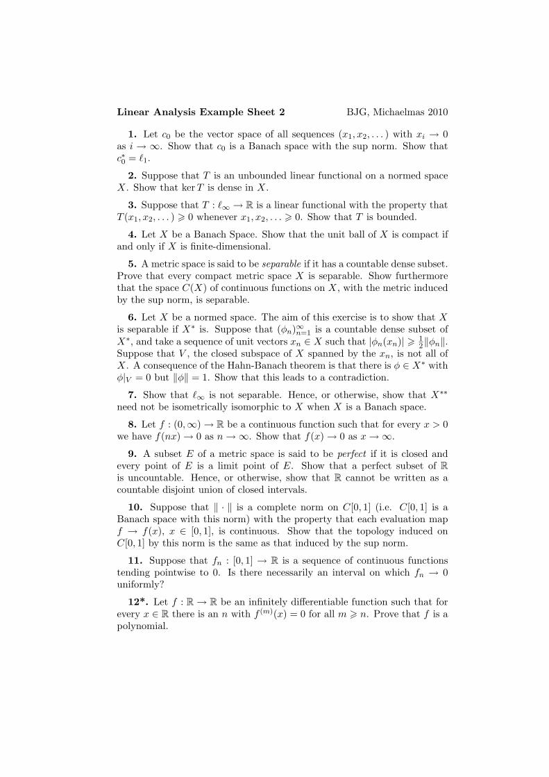
Linear Analysis Example Sheet 2 BJG, Michaelmas 2010

1. Let c0 be the vector space of all sequences (x1, x2, . . . ) with xi → 0as i → ∞. Show that c0 is a Banach space with the sup norm. Show thatc∗0 = `1.

2. Suppose that T is an unbounded linear functional on a normed spaceX. Show that ker T is dense in X.

3. Suppose that T : `∞ → R is a linear functional with the property thatT (x1, x2, . . . ) > 0 whenever x1, x2, . . . > 0. Show that T is bounded.

4. Let X be a Banach Space. Show that the unit ball of X is compact ifand only if X is finite-dimensional.

5. A metric space is said to be separable if it has a countable dense subset.Prove that every compact metric space X is separable. Show furthermorethat the space C(X) of continuous functions on X, with the metric inducedby the sup norm, is separable.

6. Let X be a normed space. The aim of this exercise is to show that Xis separable if X∗ is. Suppose that (φn)∞n=1 is a countable dense subset ofX∗, and take a sequence of unit vectors xn ∈ X such that |φn(xn)| > 1

2‖φn‖.Suppose that V , the closed subspace of X spanned by the xn, is not all ofX. A consequence of the Hahn-Banach theorem is that there is φ ∈ X∗ withφ|V = 0 but ‖φ‖ = 1. Show that this leads to a contradiction.

7. Show that `∞ is not separable. Hence, or otherwise, show that X∗∗

need not be isometrically isomorphic to X when X is a Banach space.

8. Let f : (0,∞) → R be a continuous function such that for every x > 0we have f(nx) → 0 as n →∞. Show that f(x) → 0 as x →∞.

9. A subset E of a metric space is said to be perfect if it is closed andevery point of E is a limit point of E. Show that a perfect subset of Ris uncountable. Hence, or otherwise, show that R cannot be written as acountable disjoint union of closed intervals.

10. Suppose that ‖ · ‖ is a complete norm on C[0, 1] (i.e. C[0, 1] is aBanach space with this norm) with the property that each evaluation mapf → f(x), x ∈ [0, 1], is continuous. Show that the topology induced onC[0, 1] by this norm is the same as that induced by the sup norm.

11. Suppose that fn : [0, 1] → R is a sequence of continuous functionstending pointwise to 0. Is there necessarily an interval on which fn → 0uniformly?

12*. Let f : R → R be an infinitely differentiable function such that forevery x ∈ R there is an n with f (m)(x) = 0 for all m > n. Prove that f is apolynomial.

Linear Analysis Example Sheet 3 BJG, Michaelmas 2010

1. Check carefully that if X is a locally compact Hausdorff space thenthe one-point compactification X is a compact Hausdorff space.

2. Show that if X is an infinite compact Hausdorff space then C(X) isnot compact.

3. Let f : [0, 2π] → R be a continuous function with f(0) = f(2π), andsuppose that f(n) = 0 for all n ∈ Z, where f(n) =

∫ 2π0 f(x)e−inxdx. Show

that f = 0.

4. Let X be a locally compact Hausdorff space. Show that Cc(X), thespace of continuous real-valued functions on X with compact support (thatis, {x : f(x) = 0} is compact) is dense in C0(X).

5. Let A be the collection of all functions f ∈ C([0, 1]) which are boundedpointwise by 1 and such that |f(x)−f(y)| 6 |x−y| for all x, y. Show directlythat A is sequentially compact (hint: given a sequence of functions (fi), firstpass to a subsequence which converges at every rational).

6. Show that the set of all x = (x1, x2, . . . ) ∈ `2 with |xn| 6 1/n for all nis compact.

7. Does there exist a real Hilbert space with countably infinite dimensionas a vector space over R?

8. Let {en : n ∈ Z} be an orthonormal basis for `2, and consider the set{fn : n ∈ Z}, where fn := en − en−1. Show that the linear span of {fn}is dense in `2. Is the same true if a single element is removed from {fn}?What if two elements are removed?

9. Suppose that S is a countably infinite subset of `2 with the propertythat the linear span of S′ is dense in `2 whenever S \ S′ is finite. Show thatthere is some S′ whose linear span is dense in `2 and for which S \ S′ isinfinite.

10. Show that there exists an infinite set S of unit vectors in `2 such that‖x − y‖ >

√2 whenever x, y are distinct elements of S. Can the constant√

2 be improved?

11. Show that the norm on `p is not induced from an inner product unlessp = 2.

12. Construct an inner produce space X and a proper closed subspaceY ( X for which Y ⊥ = {0}.

13 ++. By considering the function f(x) = 11+25x2 , or otherwise, demon-

strate the Runge phenomenon: there is a continuous function f : [0, 1] →R whose minimal degree polynomial interpolants at {0, 1/n, 2/n, . . . , (n −1)/n, 1} do not tend uniformly to f as n →∞.

Linear Analysis Example Sheet 4 BJG, Michaelmas 2010

1. Let p : C → C is a polynomial. Suppose that T : X → X is a boundedlinear operator on a Hilbert space. Show that the spectrum of p(T ) is{p(λ) : λ ∈ σ(T )}. Extend this result to rational functions (quotients of twopolynomials). How are the spectra of T and T ∗ related?

2. Suppose that U : X → X is a unitary map on a Hilbert space X: thatis to say, 〈Ux, Uy〉 = 〈x, y〉 for all x, y ∈ X. Show that σ(U) is contained inthe unit circle of the complex plane. By considering i(U + I)(U − I)−1, orotherwise, show that σ(U) 6= ∅.

3. Let T : X → X be a bounded linear operator on a Hilbert space.Show that if one of the maps T, T ∗, TT ∗, T ∗T is compact then they all are.

4. Let S, T : X → X be bounded linear operators on a Hilbert space.Show that if one of them is compact then ST is compact.

5. Let T : X → X be a compact self-adjoint operator on a Hilbert space.Show that there is a unique compact self-adjoint operator T+ : X → Xsuch that ‖T+x‖ = ‖Tx‖ for all x and T+ is positive in the sense that〈T+x, x〉 > 0 for all x ∈ X.

6. Let (en)n∈Z be a complete orthonormal system in a Hilbert space X,and consider the bounded linear map T : X → X which maps en to en+1.Describe σ(T ).

7. A bounded linear operator T : X → X on a Hilbert space is said tobe normal if T commutes with T ∗. Show that if T is normal then everyelement of σ(T ) is an approximate eigenvalue.

8. Is every compact operator on Hilbert space Hilbert-Schmidt?

9. Suppose that Tn are bounded operators on a Hilbert space X suchthat Tnx → 0 for all x ∈ X. Is it true that T ∗

nx → 0?

10. Is there a bounded self-adjoint operator on a Hilbert space with noeigenvalues?

11. Show that any compact set K ⊆ C is the spectrum of some boundedoperator on `2.

12. Construct a linear operator T on Hilbert space with empty spectrum.