Linear AlgebraMAT223 Course Notes - math.toronto.edu · 7 particular geometrical way of dividing up...
80
NICHOLAS HOELL LINEAR ALGEBRA MAT223 COURSE NOTES UNIVERSITY OF TORONTO
Transcript of Linear AlgebraMAT223 Course Notes - math.toronto.edu · 7 particular geometrical way of dividing up...

N I C H O L A S H O E L L
L I N E A R A L G E B R AM AT 2 2 3 C O U R S E N O T E S
U N I V E R S I T Y O F T O R O N T O

Copyright© 2017 Nicholas Hoell
published by university of toronto
www.math.toronto.edu/nhoell/mat223
Licensed under the Apache License, Version 2.0 (the “License”); you may not use this file except in compliance withthe License. You may obtain a copy of the License at http://www.apache.org/licenses/LICENSE-2.0. Unlessrequired by applicable law or agreed to in writing, software distributed under the License is distributed on an “as is”basis, without warranties or conditions of any kind, either express or implied. See the License for the specificlanguage governing permissions and limitations under the License.
First printing, September 2017

Contents
Introduction 5
What is this course about? 6
Vocabulary 9
Proofs 10
Sets 12
Expectations 14
Tips on Preparing 15
Crowdsourced Tips for Success 15
Exercises 17
Systems of Linear Equations 19
Linear Equations 20
Systems of Linear Equations 23
The Reduction Algorithm 28
Exercises 36
Geometry of Vectors 39
The Dot Product in R2 40
The Dot Product in Rn 42
Projections and Expansions 47
Exercises 49

4
The Rank Theorems 53Subspaces of Rn 54
Bases 55
Expansions and Orthogonalization 57
Rank Unification 60
Maximal Rank 66
Exercises 68
The Fundamental Theorem of Linear Algebra 71Prelude: Orthogonal Complements 72
The Fundamental Theorem of Linear Algebra 73
The Diagrams 75
Exercises 79

Introduction
Contents
What is this course about? 6
Where is this material used? 7
Examples 7
Vocabulary 9
Proofs 10
Sets 12
Expectations 14
Tips on Preparing 15
Crowdsourced Tips for Success 15
Exercises 17
This chapter provides an overview of what this course is about and theapplications in which you’ll make use of techniques encountered in thiscourse: solving systems of linear equations. As well, there’s a primer onmathematical topics and terms we expect you to know or to familiarizeyourself with as soon as possible. There are some tips from successfulstudents at the end which you may find helpful as well as advice I can offerfrom from years of experience in observing what works for students.

6
What is this course about?
This course is about one, and only one thing: solving systems of linearalgebraic equations. Of course, there’s a lot to unpack here since we’ll needto formally define the words system and linear but equally important, we’llneed to think clearly about the word solving. By that I mean it’s better todeeply understand what’s going on in trying to “solve" systems of linearequations than blindly applying algorithms, because the deep understandingallows a greater facility with modelling and, ironically, with applying knownalgorithms. Because of this fact, this course is going to involve trying tounderstand the general character of systems of linear equations throughabstracting out the more fundamental features and proving general statementsabout them rather than working through specific cases. This class is goingto force you to think differently than you may be used to thinking aboutmathematical objects since the emphasis is heaving tilted towards abstractionfor the purpose of clarity.
I should say, the goal of the course is for you to understand the followingpicture which incorporates all of the mathematical structures we’ll encounterover the course of the semester.
Figure 1: Understanding the objects in thispicture and how they relate to one another isthe ultimate aim for us this semester.
The picture above has a lot of moving parts and it will take quite awhileto reach the point where we can even precisely state what’s happening there.But in case you’re curious, the figure is a visual representation of a theorem,the fundamental theorem of linear algebra which helps us quantitativelyunderstand how linear systems, and their possible solutions, allow for a very

7
particular geometrical way of dividing up the world where “vectors" live. Ofcourse, if none of this makes sense right now - good! It’s meant only as flagfor us to point out where we’re headed as we get into some of the details insolving linear systems of algebraic equations.
Where is this material used?
Linear systems and the ideas of linearity are ubiquitous in science. As you’lldiscover in your futures in the your respective disciplines, linear algebrais the de facto lingua franca of the sciences. Why is that? I can offer twoobvious reasons.
1. Cases where Nature appears to actually be linear. I’m not sure howcommon this is but it certainly appears more as an exception than as therule. The most obvious (to me) example of this is in quantum mechanics,the branch of physics devoted to the very smallest bits of Nature. Big partsof the well-known strangeness of the picture of reality painted by quantummechanics is entirely due to the fact that Nature appears to be obeyinglinear rules.1 1 The weirdness has more to do with the
interpretations offered for the equations, theequations themselves being perfectly normal,linear differential equations. The other bigsource of weirdness is the coupling of thelinear equations with the so-called “Bornrule" for those who are interested.
2. Cases where Nature appears to not be linear. I think this is the standardsituation. When things deviate too far from linearity people tend to callthese cases “non-linear" which is a technical term meaning, basically,“hard".2 It may be surprising to you, but these are precisely the cases in
2 Strictly speaking, it often means “so hardit’s not really solvable".
which the tools of linear algebra are often the most useful. This is becauseoften a general technique of linearization is used wherein a hard, non-linear problem which cannot be solved directly gets approximated by aneasier, linear problem which can be solved. Provided the approximationsare done cleverly and carefully enough, the approximations can often giveenough of an answer as to satisfy our reasons for asking. A special case ofthis which should be familiar to you from high school calculus is the localapproximation of a function by it’s tangent line: tangent lines are “linearapproximations" to messy, complicated non-linear functions. Far morecomplicated examples abound in applications.
Examples
I want to give a few examples of places where linear algebra and the toolsfrom this course make an appearance in real-life. The list isn’t exhaustive, it’sjust places where I’ve used linear algebra, or I’ve seen linear algebra used,or I know that linear algebra happens to be used. In these examples, linearalgebra plays a big role.
1. Physics. I already mentioned quantum mechanics above. Beyond that,much of classical physics is described (or approximated) by linear laws,at various stages. Special relativity, for example, is basically a cleverapplication of tools from this class. Particle physics, the type of physics

8
making the news for the discovery of the Higgs particle for example, restson equations that can’t be understood without mastering the material inthis course.
2. Mathematics. Surprisingly, linear algebra is has applications withinmathematics itself. In fact, one enormous branch of mathematics “rep-resentation theory", is based on massively clever uses of linear algebra.The basic idea is that while the objects in linear algebra are abstract, theyhave the benefit of being very well-understood. So if one encounters amathematical object which is really abstract3 then we can study these 3 And you’d be shocked at quite how
abstract this can be!really abstract things by somehow moving them into the world of linearalgebra (at the cost of losing certain bits of informations along the way).By studying how abstract objects present themselves in linear form, youcan actually learn something about the original abstract objects. This ideais used in many foundational areas of modern mathematics.
3. Computer Science. How fast can the fastest possible algorithm reliablymultiply two arrays of numbers of increasingly large size? That question,as of this writing, remains an unsolved question in complexity theory, thediscipline of computer science dealing with optimal, idealized ways ofsolving abstract problems. How could such an easy operation, multiplyingtwo matrices, be so difficult to understand? Because every time peoplethink they’ve found the quickest way of doing it, some brilliant computerscientist notices some very clever method for shaving a little bit of workoff the total cost. Very small speedups in performance on matrix arithmetichave serious advantages since many algorithms require doing these thingson large sets of numbers repeatedly. Small gains in performance timematter, actually. A lot.
4. Google. Search engines are a type of “black box linear algebra device".The way they work rests on doing very fast matrix manipulations, some ofwhich are based on things we’ll do in this course.
5. Video Game Design. The representation of images and objects in videogames is often array-based and many of the tools we learn in this coursehave applications in the design of video games. People in this industry aremasters of this course.
6. Image Recognition. There is now software that can identify people (orcars, handwriting, whatever) in new photos based on prior images. Thisturns out to be a linear algebra problem actually.
7. Artificial Intelligence and Machine Learning. Much of what’s donenow in modern applications of artificial intelligence (self-driving cars,self-directed vacuums) and automated learning (there are computers thathave “learned" how to play perfect games of Breakout for instance) restson linear algebra. Things common to both fields, like neural networks, arebased on material we’ll do in this class.

9
8. Forecasting. I give you a list of closing prices for a tradable asset forthe past 2 weeks and I want you to estimate tomorrow’s. How do you dothis? There are many ways4 to attempt this. All the ones I know of involve 4 And, I hope this is obvious, no reliably
perfect ways.linear algebra.
9. Data Science. Any manipulations done on large data sets must meet goodperformance requirements. Keeping things linear is a good way to proceed.As well, big data is usually kept in formats where linear algebra is theobvious weapon of choice.
10. Statistics. The last four examples are, in some sense, applications ofstatistics. Then again, the entire scientific enterprise is kind of “just"statistics in the sense that statistics is the careful and quantitative analysisand inference of data, and science is simply the collection, organizationand interpretation of experimental data. You can not get anywhere instatistics without a mastery of linear algebra. Period. It is a disciplinedrenched in the language of linear algebra and probably the biggestmasters of matrices are found in Departments of Statistics.5 5 But don’t tell my colleagues in the
mathematics department I said so
Vocabulary
An enormous amount of difficulty students in this course run up against isthe correct and grammatical usage of precise terminology. The words havevery rigid usages in this course, unlike in natural languages like English. Thissimple, almost naive, observation will become fundamental as the conceptsencountered become more abstract. Moreover, misuse of very preciselydefined objects indicates a flaw in proper understanding of the underlyingconcepts. For this reason it is absolutely paramount that you are able toconvey, in written form, a clear, concise, rigorous, and correct argument usingmathematical definitions.
First off, there’s a bit of vocabulary invented by mathematicians to helpthem deal with parsing aspects of the mathematical theories they develop. Ifyou like music, there are various phrases (coda, cadenza, transition, resolu-tion, etc) which help the musicians/composers demarcate the control flowamong passages inside a single coherent composition. Here are some of theones used analogously in mathematics.
1. Theorem. This is used to indicate the big result, the ultimate goal ofintense mathematical labour. All of the deepest results in mathematicsare given this honorific.6 The general language in theorems is a statement 6 Gauss even has one which now bears the
name “Theorema Egregium" which means,roughly, “Remarkable Theorem", or “Reallybig theorem" depending on your tastes.
of assumptions (or “hypotheses") e.g. “Let A be an m × n matrix..." or“Suppose that x and y are vectors in Rn and..." followed by conclusionswhich are guaranteed true provided the hypotheses hold. The languageused in statements of theorems is famously precise and technical.
2. Lemma. A lemma is like a micro-theorem. It’s used to title results thatare somewhat interesting in and of themselves, but whose primary purpose

10
is to assist in proving theorems.
3. Proposition. This is something closer to theorem than to lemma but, well,we can’t all be theorems now can we?
4. Corollary. This is an important result which follows, using not too muchwork, from a Theorem or a Proposition.
5. Axiom. These are things we just have to take in without being able toprove. We like to keep the list of these as minimal as possible (both innumber and in cognitive complexity). Basically these are Propositions wecannot prove but simply assume. 7 7 An example of this would be the axiom
that for any two sets the collection of allthings in either of the two sets is itself a newset we can play with. Another, well-knownfrom Greek geometry, would be that all rightangles are equal. People spend entire careerstrying to see which axioms imply othersin any given system of axioms, in order topossibly reduce the “assumptive burden" ofthe system. Proving which things can or cannot be proven in any given list of axioms isan entire subfield of mathematics.
6. Proof. This is something which follows a lemma, proposition, theorem, orcorollary. It’s a formal argument designed to be incontrovertible evidenceagainst further scrutiny. If all that were known to someone were existingaxioms, and the lemmas, propositions, theorems and corollaries alreadyestablished using these axioms, then that person would be able to verify,based solely on your proof, that a given statement was true. The famedphysicist Richard Feynman once said (about science, not mathematics, butit holds here as well)
“The first principle is that you must not fool yourself – and you are theeasiest person to fool."
I encourage you to take that advice seriously. Proofs are arguments madeto safeguard against the kind of deception warned against in the quote.
Proofs
Each proof is unique since you’re proving a different statement, but thereare some common strategies you’ll encounter. For general guidelines, hereare a few thoughtlets.
(a) If the statement you’re asked to prove is something like “Prove suchand such exists." it suffices to simply exhibit an object meeting therequirements described in the statement. In other words, providing anexample constitutes a proof. Conversely, a counterexample is often usedto disprove an erroneous claim.
(b) In some cases (though not in this course) the above cannot be done,and existence is non-constructive, namely existence is establishedwithout being able to produce a single example of the object provento exist. Don’t worry about this case in this class since we won’t seethings like this, just be aware that this stuff can be subtle.
(c) Sometimes we argue by contradiction, which is to say, we assumethat the result we want to show isn’t true and use logic to arrive atsomething we know to be false. Suppose A and B are statements (calledpropositions but not to be confused with the word Proposition used

11
before as a kind of theorem!) and we are hoping to show that statementA implies statement B (written A =⇒ B symbolically). Well, since
(not B) =⇒ (not A) if and only if A =⇒ B
then if we can prove (not B) =⇒ (not A) then we can conclude theclaim we wanted to establish must be true. Make sure you understandwhy A =⇒ B is equivalent to (not B) =⇒ (not A). It may helpto think of examples “If I win the lottery, then I’ll be rich" must be thesame as “If I’m not rich, I did not win the lottery". But also notice thatthese are distinct from B =⇒ A. After all, not every rich person wonthe lottery.8 8 A little terminology here. If A =⇒ B
we say that A is “sufficient" for B and thatB is “necessary" for A. If A =⇒ B butB =⇒ A then we say “B is necessary butnot sufficient for A".
(d) Sometimes we may argue inductively. That is to say, if we want toprove a statement P(n) is true for all natural numbers n we need toshow
• P(0) is true. This establishes a “base case", i.e. the case for n = 0(or, often n = 1 or whatever).
• If P(k) is true for (k >base case) then P(k + 1) is true.
We won’t use this much but it’s there if we want it. The following is anexample of an inductive argument.
Example 1
Prove that 12 + 22 + · · ·+ n2 =n(n+1)(2n+1)
6 for n = 1, 2, 3, ...
Proof
Here P(n) is the claim that 12 + 22 + · · ·+ n2 =n(n+1)(2n+1)
6holds for positive natural numbers. Suppose n = 1. Then12 =
1(1+1)(2·1+1)6 . This gives the base case. Next, if it were
true that for k ≥ 1 we had that 1 + 22 + 32 + · · · + k2 =k(k+1)(2k+1)
6 then we would have
12 + 22 + · · ·+ k2 + (k + 1)2 =
=k(k+1)(2k+1)
6 by inductive hypothesis︷ ︸︸ ︷12 + 22 + · · ·+ k2
+ (k + 1)2
=k(k + 1)(2k + 1)
6+
6(k + 1)2
6
=k(k + 1)(2k + 1) + 6(k + 1)2
6
=(k + 1)[k(2k + 1) + 6(k + 1)]
6
=(k + 1)[2k2 + 7k + 6]
6
=(k + 1)(k + 2)(2k + 3)
6

12
which equals (k+1)((k+1)+1)(2(k+1)+1)6 , the result for k + 1.
Since P(k) =⇒ P(k + 1) we necessarily then have that P(n)holds for all n.
Caution!
A surprising number of students make serious errors when workingthrough proofs because of mixing up the hypotheses and the conclu-sion by mistakenly assuming what is to be proven! This can oftenhappen in sometimes subtle ways so let’s review.Let C be a claim we wish to prove. For instance the claim might besomething like “there are infinitely many prime numbers". We couldrestate this claim as “For every given prime number, there exists alarger prime number". Stated this way, it’s more obvious what thehypothesis and conclusion are, namely the hypothesis here is “If yougive me a prime number" and the conclusion is “There will always bea larger prime number". If I call the hypothesis P and the conclusionQ, we want to prove that P =⇒ Q and we would be wrong to assertQ without having begun at P.
Sets
A lot of the definitions and proofs in the course are phrased in the languageof sets. Sets are the primary foundational objects in mathematics. A set Sis simply a collection of elements. These elements are often indicated asan unordered list S = {s1, s2, ..., sm} say for the case of a finite set (a setwith a finite number of things in it). The real numbers R are an example ofa familiar (hopefully) set with an infinite number of elements9. So is the set 9 The real numbers are the continuum
of numbers on the number line used forgraphing functions in high school. This isthe set which contains all integers, fractions,and numbers like π, e and other numberswith non-repeating decimal expansion.
N = {0, 1, ....} of natural numbers.We use the notation #S to denote the number of elements10 in the set S .
10 Also called the cardinality of the set S .
For example #{2, 3, 5, 7, 11} = 5. By fiat we say that #S = ∞ for sets S withan infinite number of elements.
The primary relationship used to describe sets is membership, denotedby the symbol ∈ or its negation < read as “in" or “not in", respectively. Thissymbol is used to indicate that an element is in a given set: namely, s ∈ Smeans the element s is a member of the set S . These symbols can be orientedin a reversed way as 3 and = so that
s ∈ S ⇐⇒ S 3 s
In other words, the above are equivalent statements.Often, the sets we encounter in this course are described by listing condi-

13
tions inside the defining brackets of the set. For example
Q = {pq| p, q ∈N, q , 0}
describes the set of rational numbers. Notice, in the above, that the verticalline | (some people use colons instead of vertical lines) separates the lefthand side, which gives a description of the elements, from the right handside, which gives a restriction on the things appearing on the left hand side.Notice, in the above, p, q don’t really exist since they represent placeholdersfor numbers which meet some restrictive criteria: if I were to replace them inall occurrences, I would still have the same set description, namely
{pq| p, q ∈N, q , 0} = {
sr| s, r ∈N, r , 0}
are both perfectly valid descriptions of the set Q. This property of the vari-ables appearing in the sets above, that the variables can be replaced by anyother unused variable provided the replacement is done in all occurrencesof the variable, is termed binding and the variables are said to be boundvariables. A misunderstanding of the differences between free and boundvariables is a source of constant trouble for many MAT223 students. If youare confused - don’t wait to get unconfused because this issue is crucial inunderstanding the concepts throughout the semester.
As well, there are a few natural binary operations11 The first one is the 11 Operations which takes two operands, inthis case two sets.union operation, denoted ∪. Unioning two sets S 1, S 2 creates a new set
S 1 ∪ S 2 containing all elements which appear in either set S 1 or S 2 or both.The way we write this fact is
S 1 ∪ S 2 = {s | s ∈ S 1 or s ∈ S 2}
Another natural binary operation is the intersection operation ∩ which takestwo sets S 1, S 2 and creates a new set S 1 ∩ S 2 containing elements whichappear in both S 1 and S 2.
In addition to the above there are binary inclusion relationships. Forinstance S 1 ⊂ S 2 means that S 1 is a subset of set S 2. What that means is thateverything in S 1 must also be in S 2. Namely
s ∈ S 1 =⇒ s ∈ S 2, for all s ∈ S 1
Establishing that implication above, for an arbitrary element s ∈ S 1, is allthat’s required to show that S 1 ⊂ S 2. Here I want to make an importantpoint about notation: different people prefer different conventions, and someauthors prefer the notation S 1 ⊂ S 2 to generally indicate that S 1 is a propersubset of S 2, namely that S 1 is not actually equal to S 2. Those authorsmay use notation like S 1 ⊆ S 2 to indicate the neutral position, not makingassumptions about whether S 1 is a proper subset or not. But many authors(the majority) use the notation ⊂ and ⊆ interchangeably and will use the

14
notation S 1 ( S 2 to denote that S 1 is a subset contained in, but not equal to,set S 2. All of these notations have their reversed counterparts ⊃,⊇,) whichsimply reverse the inclusion relationship to be read from right to left.
When are two sets equal? Clearly, when they have the same elements. Inother words S 1 = S 2 must means that everything in set S 1 must appear in setS 2, i.e. S 1 ⊆ S 2 and everything in set S 2 must appear in set S 1 i.e. S 2 ⊆ S 1.In other words
S 1 = S 2 ⇐⇒ S 1 ⊆ S 2 and S 2 ⊆ S 1
This is a standard approach to showing two sets are equal which we’ll usethrough the semester so make sure you understand what it says and why it’svalid.
Two final comments about sets. First, there’s a (somewhat pathological)set that appears as a subset of every set - namely, the empty set. The emptyset, denoted ∅ (or {}) is what its name implies, it’s a set with no elements.Its utility is there for reasons of mathematical consistency well beyond thescope of what we will encounter in this course. Note well that ∅ is the onlyset satisfying #∅ = 0. Secondly, there’s an operation called complementing,which given a set S produces a set S c called the complement of S . S c is a setwhose elements are all elements not appearing12 in S . For instance, what is 12 A subtle point: the idea of taking
complements raises the question of towhich ambient set are we referring? Forinstance, is ∅c = N or R or something elsealtogether? For the most part, the contextis clear and so this isn’t an issue. Whencomplete clarity is needed, the notationS 2 \ S 1 will be used. S 2 \ S 1 means allelements in S 2 which are not in S 1. Thisindicates that S 2 is the ambient set for whichto take complements.
Qc? Well, it should be all numbers not expressible as ratios of integers. Inother words, it’s the set of irrational numbers. So we have π ∈ Qc,
√2 ∈ Qc,
etc.
Expectations
In general we expect complete facility with the logic of things like “A =⇒
B is equivalent to (notB) =⇒ (notA)" on tests and quizzes. In other words,basic logic and solid reasoning is what we expect of you.
That said, of course we don’t expect you to be able to prove super hardthings on quizzes or tests so you shouldn’t stress too much. Most of what wewill ask for in a conceptual or proof-style question on a test can be done inonly a few lines, just a short, rigorous explanation which correctly appliesdefinitions or known theorems. Often, amazingly, performing a rigorousargument isn’t a whole lot harder than being able to write down a definitionand think about what it actually means, and think through the consequencesof the assumptions you’ve been given.
As well, you may be asked to give definitions of things we’ve gone overin lecture or in homework. These should be easy, free points. All we ask isto restate a definition. It’s our way of checking that you are paying attentionand really internalizing the concepts. But, of course, the definition has to beprecise and correct!

15
Tips on Preparing
I haven’t discovered some new, super-fancy and stress-free way of masteringmathematics. All I can offer are a few, very general suggestions. They dowork, but you actually have to do them in order for them to work. Mostpeople end up trying to “yeah, yeah" and cut a few corners. What you do withmy well-meant suggestions is up to you.
1. Working with friends can help a lot. It can help because it gives you theopportunity to explain your reasoning, out loud, to another person. You’dbe surprised how helpful that can be.
2. Working all the suggested problems. Mathematics isn’t a spectatorsport. The only thing that makes you better is practice, practice, practice.
3. Not getting behind. The semester moves fast. It’s very easy to procrasti-nate and fall behind on homework. It’s a recipe for disaster in a course likethis because cramming won’t help much. Staying on schedule and beingdiligent with the homework requires discipline but it’s worth it.
4. Don’t miss tutorials. Exiting course grades are strongly correlated withattendance in tutorials and performance on quizzes. Not attending tutorialsis a very reliable predictor of poor final grades.
5. Use the class Piazza. It’s there for you to ask questions and learn fromeach other. I wish it had been around when I was a student.
6. Try to make time each day to work on MAT223 related things. Thiscould be as easy as reading the book for 20 minutes every other day anddoing problems in the days between. If you can find a routine whereyou reliably spend a portion of each day working problems, thinkingthrough concepts, reading material, etc. you’ll find your ability to retainthe information greatly enhanced.
7. Get enough sleep. You’d be amazed at the benefits of sleep. I tried veryhard as an undergrad to sleep a lot, especially before any tests. In general,the mental sharpness a good night’s sleep gave far outweighed any littlecramming I’d get by staying up too late.
8. Try reading ahead. If you read a few pages of the next lecture’s topic, itoften improves your ability to follow the lecture.
Crowdsourced Tips for Success
An excellent question was asked on Piazza in Fall, 2016. I’m sharing it and afew of the responses it received since I consider the advice therein to be veryhelpful. Here was the original posting.13 13 Forgive the small font, it happens to be
the only way to have a reasonable lookingimage but it’s admittedly hard to read.

16
And here’s the first answer posted, which indicates the diligence typical ofstudents who perform well on hard tests.
Then I chimed in with my two cents.
And there was another commenter with additional ideas.
And, lastly, a voice from one of the 3 students who earned a perfect scoreon midterm 2. As in my own thoughtlets before, there isn’t really a “royalroad" here. There’s just hard work and the ability to stay calm in a testenvironment. Being prepared is one of the best ways to remain calm.

17
I encourage you to study the success stories carefully and glean what youcan from them. The big takeaway is that doing well requires a lot of work,and a strong desire to succeed. Good luck in your studies!
Exercises
Do the following exercises offline.
1. Describe the sets {x ∈ R | x2 = k, k ∈N} and {x, y ∈ R | x
y = 2, y , 0}
2. Describe the set {x ∈N | x , kl, k, l ∈N, k < x, l < x, k , 1, l , 1}
3. Write down a definition of S 1 ∩ S 2 using set notation.
4. Show that (S 1 ∩ S 2)c = S c1 ∪ S c
2 holds for all sets S 1 and S 2.
5. Show that (S 1 ∪ S 2)c = S c1 ∩ S c
2 holds for all sets S 1 and S 2.
6. Prove that (S 1 ∩ S 2) ⊂ (S 1 ∪ S 2) holds for all sets S 1 and S 2.
7. Are the notations {s} ⊂ S and s ∈ S interchangeable? Why or why not?
8. Prove that for any subset T of set S , we have S = T ∪ T c
9. Here’s a claim: S = T ⇐⇒ #S = #T . If true prove it. If false, give acounterexample.
10. Use induction to prove that 1 + 2 + · · ·+ n =n(n+1)
2 for all positiveintegers n.
11. Use induction to prove that 2 + 22 + · · ·+ 2n = 2n+1 − 2 holds for alln > 0.
12. Use induction to prove that 7n < 8n+1 holds for n ≥ 0, n ∈N
13. Use induction to prove the following claim: Every nonempty subset ofN has a smallest element.

18
14. Consider a set S . We define a new set, P(S ) = {all subsets of S}.
• Write down P({0, 1}).
• Write down P({0}) and P(P({0}))
• Use induction to prove that #P(S ) = 2#S holds for all sets with#S < ∞
15. (Harder). Consider the set S = {s | s < s}. Is this set well-defined? Whyor why not?
16. (Harder). Use induction to prove that 8n − 3n is divisible by 5 for n > 0
17. (Harder). Consider a well-known incorrect use of induction used to“prove" the false claim that cars are all the same colour. The “proof" goeslike this:
The claim is that cars are all the same colour. This is equivalent to theclaim that any set of cars must contain cars of the same colour. The claim istrivially true for the base case of n = 1 cars since, after all, a car has onlyone colour.14 Next, we’ll assume that the claim is true for all sets of n cars 14 Though this isn’t true for real cars, we’ll
actually pretend this is true for cars here.In other words this line is not where themistake happens.
are we’ll now consider a set of n + 1 cars, {car 1, car 2, ..., car n, car n + 1}.We’ll consider two subsets of this set C1 = {car 1, car 2, ..., car n} andC2 = {car 2, ..., car n, car n + 1}, each of which is a set of n cars. Therefore,by our induction hypothesis, C1 and C2 only contain cars of a single colour.But then again, since there’s overlap in the entries of C1 and C2 the colourof each must be the same. Therefore {car 1, car 2, ..., car n, car n + 1} musthave only cars of a single colour. Thus, cars are all of the same colour.
What went wrong with the above “proof"?
18. (Harder). In a previous question you were asked to use induction to showthat every nonempty subset of N has a smallest element. Now show theconverse. Namely show that if the claim that every nonempty subset of N
has a smallest element is a true fact about set the N, then induction is avalid method of proof.

Systems of Linear Equations
Contents
Linear Equations 20
Parameterized Solutions 21
General Linear Equations 23
Systems of Linear Equations 23
Equivalence 25
The Reduction Algorithm 28
The Reduction Algorithm 32
Exercises 36
This chapter introduces you to the main subject of study in this course:systems of linear equations. We derive some elementary facts about suchsystems and develop a rigorous procedure for solving the solvable ones.

20
Linear Equations
This course is about solving systems of linear algebraic equations. We’llbe dealing with methods of abstracting the fundamental concepts which arecrucial in understanding such systems. In order for this to be comprehensible,we’ll need to have a completely thorough understanding of the concretespecifics on which the abstraction in based.
With that in mind, let’s first recall that a single linear algebraic equation, invariables x and y is an equation like
ax + by = c
In the above, x, y are variables while the numbers a, b, c are coefficients. Asthe coefficient c doesn’t appear as being multiplied by a variable, we give ita special name and refer to it as the constant term. Often we place constantterms on the right hand side of the equals sign. If the constant term c = 0 wecall the equation homogeneous.
In general, coefficients are givens, in the sense that we cannot changetheir explicit values whereas the variables are unknowns because they areplaceholders for numbers we’d like to determine. Therefore, we often refer tothe above as one equation in two unknowns. For example,
x − 2y = 5
has a = 1, b = −2 and c = 5. All this is just to remind you that theletters we’ll use to represent coefficients are fixed values whereas generallythe letters we use to represent variables are meant to be unknown but notnecessarily fixed values.
By a solution to a linear equation like the above we mean an assignmentof values to the variables resulting in a valid equality. For instance, theassignment of x = 3 and y = −1 in the above yields 3 − 2(−1) = 5. In thisexample the assignment x = 3, y = −1 works as well. In fact, this exampleactually has infinitely many solutions as we can see by rewriting it as
x = 5 + 2y
In this form notice that each value we assign to the variable y, by constructionmust result in a valid assignment of a value for x. In other words, you cannow immediately see that, for instance, if y = 17 then x = 5 + 2(17) = 39so x = 39, y = 17 must be a valid solution to the original equation. 15 15 Notice that writing it this way is equiv-
alent to writing x = f (y), viewing x as afunction of y.
By a solution set to a linear equation we mean the collection of all possiblesolutions. For instance, the solution set to the equation x − 2y = 5 is
{(x, y) | x = 5 + 2y, y ∈ R}
which is the set of all pairs of numbers satisfying the constraint that the firstnumber in the pair is always 5 plus twice the second number in the pair.

21
Phrasing things this (overly verbose) way should highlight that we may alsowrite the solution set above as
{(x, y) | x = 5 + 2t, y = t, t ∈ R} (0.0.1)
a point we focus on in the next section.A final remark. In high school, you’ll recall that the solution set for linear
equations like −mx+ y = b is visually represented as the graph of the functiony = f (x) = mx + b. While this visual reminder is helpful early one whenwe increase the number of variables it can become much harder to visualizesolution sets.
Parameterized Solutions
We can express the relationship between y and x implicitly expressed in theequation x = 5 + 2y by writing the solution in so-called parameterized formas x = 5 + 2t
y = t, t ∈ R
Where, in the above, we’ve introduced a parameter t ∈ R, which implicitlyvaries over an infinite range of values.16 Namely, t = 1, t = −3, t = π 16 Take a moment to compare the above with
(0.0.1) to verify that they are equivalent.give three different values of pairs (x, y) each of which solves the originallinear equation. We refer to the parameterized solution above as the generalsolution to the linear equation as every particular solution like x = 3, y =
−1 can easily be obtained from the general solution by using a particularchoice of parameter.
Definition 1
A parameterized solution to a linear equation is a solution written interms of one or more parameters. Parameters are variables presumedto vary over a given range of values, each of which gives a validsolution to the original linear equation.
As the definition indicates and the next example clarifies, parameterizedsolutions may well consist of multiple parameters.
Example 2
Find the general solution, in parametric form, to the linear equation inthree unknowns 2x − 3y + 6z = 19.Solution: We pick a variable (in this case x) to stay on the left handside of the equals sign and move all others to the right giving
2x = 19 + 3y − 6z
Diving by the coefficient on x gives us x = 192 + 3
2 y − 3z. Finally, wecan introduce two parameters t, s to write the parameterized solution

22
as x = 19
2 + 32 t − 3s
y = t
z = s
for s, t ∈ R
The utility of the above is that we can set t and s to be any numbers wewish and plugging them into the formula will immediately yield a validassignment of values to variables x, y, z. For instance, t = 2, s = 1 gives,x = 8, y = 2, z = 1 as one particular solution to the linear equation.
In the previous example there was nothing canonical about the choice of xas staying on the left hand side of the equals sign. We could just as well havewritten the parameterized solution as, say,
x = t
y = − 193 + 2
3 t + 2s
z = s
for t, s ∈ R. Another important remark is that the parameters are logicallybound variables17 which means that they may be replaced by different 17 Make sure you understand the discussion
about free versus bound variables in theIntroduction.
variables, provided the replacement is made in all occurrences, if you wish.For example, in the above example we’d obtained
x = 192 + 3
2 t − 3s
y = t, t ∈ R
z = s, s ∈ R
But we can use a new parameter t = 32 t and s = −3s to give an equivalent
general solution to the same problemx = 19
2 + t + s
y = 23 t, t ∈ R
z = − 13 s, s ∈ R
This is a subtle and important point which will recur throughout the course- if t, s are arbitrary numbers, then so must be t = c1t and s = c2s for anynonzero c1, c1so there cannot be a unique parametric form for the generalsolution to a linear equation.
In fact, having done such a change of parameters doesn’t warrant givingthe parameters new symbols! We often prefer to simply write
x = 192 + 3
2 t − 3s
y = t, t ∈ R
z = s, s ∈ R
describes the same solution set as
x = 19
2 + t + s
y = 23 t, t ∈ R
z = − 13 s, s ∈ R

23
Notice that we use the same symbols t, s in both parameterized forms ofthe general solution without any problems since, owing to the fact that theparameters are bound variables, they are simply placeholders for particularnumbers and therefore don’t have intrinsic values associated with them.Again, this is often a point of confusion for many students so please reviewthis example carefully.
General Linear Equations
We can generalize the simple examples described in the previous section byincreasing the number of variables and coefficients in a linear equations. Todo this we often write things like
a1x1 + a2x2 + · · ·+ anxn = b
for a linear equation in n variables x1, ..., xn. We also call this one equation inn unknowns. As we’ve done before we have the constant term b on the righthand side of the equals sign. If b = 0 we call this equation homogeneous.We use subscripts on coefficients and variables since otherwise for equationswith lots of variables we’d quickly run through the alphabet and not haveenough symbols. We say that the equation is consistent if it has at least onesolution and inconsistent otherwise. For example, the linear equation x − 2y =
5 is consistent since, as we already saw, it has infinitely many solutions(which we can describe using a parameterized form for the general solution).You might be wondering how a linear equation could be inconsistent. To seehow this could happen consider a simple equation of the form ax = b witha = 0 and b = 1. Clearly no value of x could solve such an equation sotherefore the equation must be inconsistent.
Systems of Linear Equations
A system of linear equations is precisely what its name implies - namely, acollection of linear equations in the same unknown variables. For example
x − 2y = 57x + 15y = 6
(0.0.2)
is a linear system of two equations in the two variables x, y.Generalizing this, we have a system of m linear equations in n unknowns,
generally takes the form
a11x1 + a12x2+ · · · +a1nxn = b1
a21x1 + a22x2+ · · · +a2nxn = b2...
......
am1x1 + am2x2+ · · · +amnxn = bm
(0.0.3)
In the above, we’re using double subscripts like ai j to denote the coefficientof variable x j appearing in the ith equation. In general of course, the order

24
matters - i.e. a31 , a13 etc. We can unambiguously reference the coefficientsin such a system by the notation ai j, 1 ≤ i ≤ m, 1 ≤ j ≤ n. We may referto the coefficient ai j as the (i, j)′th coefficient of the system. As well, thecoefficients appearing on the right, b1, ..., bm are the constant terms. If theconstant terms are all zero, then the linear system is homogeneous.
The important thing is that the variables x1, x2, ...xn are the same in allequations. Each equation in (0.0.3) can be seen as imposing an additionalconstraint on the allowed values for the variables x1,...,xn, since in generaladding new equations can never serve to increase the possible numbers ofsolutions to the system. As with linear equations, by a solution to a linearsystem of equations we simply mean a particular assignment of values tothe variables such that all equations in the system are valid. Of course, thecollection of all possible solutions to a given system of equations is called thesolution set of the system. Notice that this definition allows for the solutionset to be empty. If there is one, and only one, solution in the solution setfor a given linear system, then we say the solution is unique. These aresummarized below.
Definition 2
A linear system is said to be
• Consistent if there is at least one solution in the solution set
• Inconsistent if there are no solutions
Moreover, we say that the solution is unique if it is consistent andthere is one and only one solution solution in the solution set. If thesystem is consistent but there is more than one solution, we say that agiven solution is not unique.
The following is a fundamental result characterizing the nature of consis-tency of solutions to systems of linear equations.
Theorem 1
A linear system of equations
a11x1 + a12x2+ · · · +a1nxn = b1
a21x1 + a22x2+ · · · +a2nxn = b2...
......
am1x1 + am2x2+ · · · +amnxn = bm
can only have 0, 1 or infinitely many solutions.

25
Proof
If the system of equations is not solvable then it definitely has 0solutions and there’s nothing left to prove. So suppose that thesystem of equations is consistent and that the solution set is S . If#S = 1 then, yet again, there’s nothing left to prove. So let’sconsider the case of #S > 1. In other words, suppose that thereare two distinct elements s1, s2 ∈ S , where s1 , s2. Each so-lution, s1 say, is just a set of values for the variables in the lin-ear system, i.e. s1 = {x1 = c1, x2 = c2, ..., xn = cn} ands2 = {x1 = d1, x2 = d2, ..., xn = dn} where ci , di for at leastone i. But then now we can define
s3 = {x1 = k1c1 + k2d1, x2 = k1c2 + k2d2, ..., xn = k1cn + k2dn}
for any choice of nonzero numbers k1, k2 such that k1 + k2 = 1. Youcan easily verify that s3 ∈ S and s3 , s1, s3 , s2. Noticewe can select infinitely many choices of nonzero k1, k2 such that k1 +
k2 = 1 so therefore there are infinitely many more ways to select ele-ments like s3. Thus, #S = ∞ and the result is proved. �
Equivalence
Our strategy in solving systems of linear equations is to perform variousmanipulations on them in order to transform them into equivalent, but simplerto solve, systems. The following definition gives us the right manipulations toattempt.
Definition 2: Equivalent Systems
Two systems of linear equations are said to be equivalent if, and onlyif, they have the same solution set.
Making this concrete, let’s consider (0.0.2). We already saw that thefirst equation in (0.0.2), x − 2y = 5, has infinitely many solutions, whichwe were able to produce in a simple parameterized form. However, not allof those solutions will be solutions to the full system (0.0.2). For instancex = 1, y = −2 solves the first but not the second of the equations in thesystem. To try to solve a system like (0.0.2) we recall a few observationsabout manipulations of simultaneous algebraic equations from high school.

26
Definition 3: Elementary manipulations of systems
For a system of linear algebraic equations
a11x1 + a12x2+ · · · +a1nxn = b1
a21x1 + a22x2+ · · · +a2nxn = b2...
......
am1x1 + am2x2+ · · · +amnxn = bm
we can always
1. Swap the order of any two equations (called interchange)
2. Multiply both sides of any equation by a nonzero constant (calledscaling)
3. Replace an equation with the result of adding a multiple of it andanother equation (called replacement)
The set of solutions to the system of equations which results fromany of the above elementary manipulations is the same as the set ofsolutions to the original system (the systems are equivalent).
The way that we systematically solve systems of linear equations is bycareful and successive application of the allowed equation manipulationslisted above so that the system appears in a nicer for than it began. The nextexample illustrates this in detail.
Example 3
Solve system (0.0.2)x − 2y = 5
7x + 15y = 6
by use of elementary equation operations.Solution Let’s begin by replacing the current second equation with
new second equation = −7 × (first equation) + second equation
This results in the system
x − 2y = 50x + 29y = −29
Next we apply the scaling operation
new second equation =1
29(second equation)
to get the systemx − 2y = 5
y = −1

27
We’ll perform one last elementary manipulation of the rows by replac-ing the first row with the result of adding the first equation and twicethe second equation as in
new first equation = first equation + 2(second equation)
The result of which yields
x = 3
y = −1
which, as you can check, solves the original system of equations.
Make sure you heed the following caution about correct manipulations oflinear systems.
Caution!
You’ll notice that nowhere in the list of elementary equation manip-ulations is there a rule saying something like “put one variable interms of another and substitute that variable into another equationand..." Often, students learn to solve a simple system by means ofsuch substitution techniques. This is NOT how we solve systems oflinear equations in general.For instance, it would be wrong (and result in no points on an exam)to try to solve
x − 2y = 57x + 15y = 6
by saying
x − 2y = 57x + 15y = 6
=x = 2y + 5
7x + 15y = 6
=⇒ 7(2y + 5) + 15y = 6
=⇒ (14 + 15)y = 6 − 35
=⇒ y = −2929
= −1
=⇒ x = 2(−1) + 5 = 3
The above “method" for solving the linear system is not allowed inthe course. The reasons for why it’s not a reliable method will, hope-fully, become obvious as the course progresses. The only methodswe may use to solve systems of linear equations right now are thoseoutlined in the Elementary Manipulations of Systems.
Of course, just like with single equations we may encounter parameterizedsolutions when solving systems of equations as the next example illustrates.

28
Example 4
Solvex + y + 7z = 05x + y − z = 8
.
We begin with a replacement operation, subtracting 5 times the first
row from the second row resulting inx + y + 7z = 0−4y − 36z = 8
. We can
then perform a scaling operation on the second equation by dividing it
by −4 which givesx + y + 7z = 0y + 9z = −2
. Then we use a replacement
operation to subtract equation 2 from equation 1 yielding
x −2z = 0y + 9z = −2
At this point we can see that both x and y variables can be solvedfor in terms of the variable z so we can write the solution set in thefollowing parameterized form
x = 2t
y = −2 − 9t
z = t, t ∈ R
Since the system is solvable we say the system is consistent. Becausethe solution set is infinite, the solution is not unique.
The Reduction Algorithm
We’re going to systematize the method we introduced in the last section forattempting to solve systems of linear equations. Let’s begin by noting thatwhen give a system like
x − 2y − 4z = 57x + 15y + 2z = 6x + 3y − 12z = 0
we can concentrate on the coefficients by considering the array of numbersmaking up the system, namely,
1 −2 −4 57 15 2 61 3 −12 0
referred to as the augmented matrix of the linear system. Each row of theabove matrix18corresponds to an equation in the original system. The first 3 18 Matrix in this context simply means a
two-dimensional array of numbers.columns of the above matrix correspond to variables in the original system,whereas the 4th column corresponds to the constant terms. For the purposes

29
of trying to solve a linear system it’s enough to work with the associatedaugmented matrix. The array of numbers
1 −2 −47 15 21 3 −12
is the coefficient matrix for the system and
560
is the constant matrix for the
system. Thus, the augmented matrix is the coefficient matrix and the constantmatrix for a system separated by a vertical line.19 19 Many authors choose not to include the
vertical line since the constant matrix alwaysappears as the rightmost column of theaugmented matrix.
It’s easier to work with numbers rather than with equations. Since eachrow of the augmented matrix associated to a linear system is an equation ofthe system, our elementary manipulations of systems from last section cannow be restated in terms of operations on rows of matrices.20 20 The plural form of matrix is matrices.
Definition 4: Elementary Row Operations
The following are called elementary row operations on a matrix.
1. Swap the order of any two rows (called interchange)
2. Multiply a row by a nonzero constant (called scaling)
3. Add any multiple of one row to a different row (called replace-ment)
Performing any of the above elementary row operations to an aug-mented matrix for a linear system produces an augmented matrix foran equivalent system.
Any two augmented matrices whose linear systems have the same solutionset are said to be equivalent (or row equivalent). Clearly elementary rowoperations produce equivalent matrices. We indicate that two matrices, A andB are equivalent by the notation A ∼ B.
Let’s go back and revisit an earlier example from the point of view ofaugmented matrices.
Example 5
Solvex − 2y = 5
7x + 15y = 6
by use of elementary row operations on the associated augmentedmatrix.The corresponding augmented matrix is1 −2 5
7 15 6

30
We can apply a replacement operation by adding −7 times row 1 torow 2, which will give us the opportunity to use a nice notation aswell. 1 −2 5
7 15 6
R2−7R1−−−−−−→
1 −2 50 −29 −29
Then we perform a scaling operation, followed by another replace-ment operation.1 −2 5
0 29 −29
129 R2−−−−→
1 −2 50 1 −1
R1+2R2−−−−−−→
1 0 30 1 1
The system above corresponds to
x = 3y = 1
so we can simply read
off the solution.
In the last example we used a helpful bookkeeping system to indicatewhich elementary row operation we performed. Namely we used arrows
with row combinations above them. For instanceR4−5R2−−−−−−→ would indicate
replacing row 4 by row 4 minus five times row 2. Swapping two rows could
be indicated by, say,R2↔R5−−−−−−→ which would mean interchange rows two and
five.Caution!
Be careful when using elementary row operations to avoid combiningmultiple operations into a single step. Namely, when performing asequence of elementary row operations, get in the habit of doing themone at a time. Namely, instead of1 0
0 1
→ 0 57 0
The above should be indicated as being the following sequence1 0
0 1
R1↔R2−−−−−−→
0 11 0
5R1−−−→
0 51 0
7R2−−−→
0 57 0
Whether or not a matrix is considered an augmented matrix, we’re going
to look at an algorithm for solving a system by applying a sequence of rowoperations to a corresponding matrix. For this, we begin by characterizinga “nice" form for matrices. Namely, in the preceding example, we ended up
with the “nice" matrix1 0 30 1 1
which has a form allowing us to simply
read off the values of the associated variables. Our goal is to develop asystematic procedure for applying elementary row operations to matricesto get them into this kind of “nice" form so we can immediately read off
solutions, if they are solvable, or determine if the solution is inconsistent

31
otherwise.We say that a row is a zero row if every number in that row is zero. As
well, we call the first nonzero entry in a nonzero row the leading entry forthat row.
Definition 5: Row Echelon and Reduced Row Echelon Form
A matrix is said to be in row echelon form or REF if it satisfies
1. Any zero rows appear at the bottom of the matrix
2. The leading entry in a given nonzero row appears in a column tothe right of the leading entry in the row above it (if any).
3. All entries (if any) in a column below a leading entry are zero.
Furthermore, a matrix is said to be in reduced row echelon form orRREF if it’s in row echelon form and additionally satisfies
1. All (if any) leading entries are 1.
2. Each leading 1 (if any) is the only nonzero entry in its column.
The above is a lot to absorb so give it some thought. While being cumber-some to state it has the power of being very precise. So precise, in fact, that acomputer can readily verify whether a given matrix is in RREF.
Example 6
We use the convention that � is an arbitrary nonzero number (i.e.leading entry) and ∗ shall denote any number. Then, as you canverify,
� ∗ ∗ ∗
0 0 � ∗
0 0 0 0
and 0 � ∗
0 0 0
are both in REF.The matrices 0 1 ∗ 0
0 0 0 1
,
1 ∗ 0 ∗
0 0 1 ∗
0 0 0 00 0 0 0
are in RREF. These example illustrate the more general fact that REFand RREF matrices have a “staircase" like pattern to them.
It turns out (though we will not prove it) that every matrix is equivalentto a matrix in reduced echelon form. In other words, given any matrix, there

32
exists a sequence of elementary row operations you can apply to it whichwill, in the end, result in a matrix in RREF. Notice that this fact implies thatto each matrix, there are special positions, called pivot positions which arelocations of leading entries in the RREF of a given matrix. For example,the matrix
0 0 41 0 20 0 0
has pivot positions, indicated by �, in the locations
� 0 00 0 �
0 0 0
, namely in
the (1, 1) and (2, 3) spots. Similarly, pivot columns of a matrix are columnscontaining pivot positions. So, in the preceding example, columns 1 and 3are pivot columns. Notice that, in this example, 0 can occupy a pivot positionsince pivot position is defined by the equivalent reduced form of a givenmatrix, not necessarily by the current form of the matrix.
The Reduction Algorithm
We can now describe an algorithm which will be used to determine if a givenlinear system is consistent and, if so, what it’s solution set it. Namely, thealgorithm will find a matrix’s unique RREF form by using elementary rowoperations.
Definition 6: Reduction Algorithm
Apply the following to A in order to produce the unique RREF matrixequivalent to A.
1. Select the leftmost nonzero column, if one exists. This is a pivotcolumn. If none exists, the matrix is already in RREF, so stop.
2. Select (possibly using row interchanges) a nonzero entry from thispivot column to place into the pivot position. This entry is called apivot.
3. Use replacement operations to produce zeros in the pivot columnbelow the pivot.
4. Apply the above steps 1–3 on the submatrix of rows to which theabove has not already been applied.
After applying the above, the matrix will be in REF. Since, at eachpass through steps 1–3 a new leftmost column is selected, this iscalled the forward phase of the algorithm. Now to get it into RREFwe must apply the backwards phase to the output.
1. Select the rightmost pivot position, if one exists. If needed, use

33
a scaling operation to ensure that the pivot occupying the pivotposition is 1. If none exists, stop.
2. Use replacement operations with the pivot you’ve selected tocreate zeros above the pivot.
3. Apply the above two steps on the submatrix of rows for which theabove has not yet been applied.
The following demonstrates the algorithm.
Example 7
The algorithm can be applied to any matrix but for this example, we’ll
apply it to the augmented matrix
1 −2 0 57 −8 1 52 8 5 −53
. To begin, the
first column happens to be the leftmost nonzero column. It’s pivot po-sition already contains 1 as a pivot. We apply replacement operations,using that pivot to create zeros in the pivot column.1 −2 0 57 −8 1 52 8 5 −53
R2−7R1−−−−−−→
1 −2 0 50 6 1 −302 8 5 −53
R3−2R1−−−−−−→
1 −2 0 50 6 1 −300 12 5 −63
Next, we apply the algorithm to the submatrix
6 1 −3012 5 −63
, namely
we have 1 −2 0 50 6 1 −300 12 5 −63
R3−2R2−−−−−−→
1 −2 0 50 6 1 −300 0 3 −3
We next apply to algorithm to the submatrix
[3 | −3
]for which there’s
nothing to apply. So we have now completed the forward phase.
Notice that our resulting matrix,
1 −2 0 50 6 1 −300 0 3 −3
is in row echelon
form. We proceed to the backwards phase. The rightmost pivot is theelement 3 in the third column.1 −2 0 50 6 1 −300 0 3 −3
13 R3−−−→
1 −2 0 50 6 1 −300 0 1 −1
R2−R1−−−−−→
1 −2 0 50 6 0 −290 0 1 −1
Now we go through the steps again with the next most rightmost

34
pivot, which happens to be the 6. This gives1 −2 0 50 6 0 −290 0 1 −1
16 R2−−−→
1 −2 0 50 1 0 − 29
60 0 1 −1
R1+2R2−−−−−−→
1 0 0 5 − 29
30 1 0 − 29
60 0 1 −1
which equals
1 0 0 − 14
30 1 0 − 29
60 0 1 −1
. Applying the algorithm one last time
to the last remaining pivot we see that it’s already a 1 and we can stop.
Notice that the result
1 0 0 − 14
30 1 0 − 29
60 0 1 −1
is in RREF.
The prior example illustrates the utility of the reduction algorithm insolving linear systems. Namely, to solve the linear system
x −2y = 57x −8y +z = 52x +8y +5z = −53
we simply apply the reduction algorithm to the associated augmented matrix,1 −2 0 57 −8 1 52 8 5 −53
∼1 0 0 − 14
30 1 0 − 29
60 0 1 −1
which in this case corresponds to
x = − 143 , y = − 29
6 , z = −1.Suppose that we have applied the reduction algorithm to an augmented
matrix for a linear system and the result is, say,1 0 2 60 1 5 70 0 0 0
Which corresponds to the system of equations
x +2z = 6y +5z = 7
The variables, x and z which appear in the pivot columns are referred to asbasic variables (sometimes also called a leading variable) while the variablein the non-pivot column, y is a free variable. We’ve seen how to deal withcases like this before, namely we expressed the solutions in terms of aparameter by expressing the basic variables in terms of the free variables.Namely, the solution set is given by
x = 6 − 2t
y = 7 − 5t
z = t, t ∈ R

35
Definition 7: Solving Systems by Reduction Algorithm
Given a linear system
a11x1 + a12x2+ · · · +a1nxn = b1
a21x1 + a22x2+ · · · +a2nxn = b2...
......
am1x1 + am2x2+ · · · +amnxn = bm
construct the corresponding augmented matrix [A | b], where A is thecoefficient matrix of the system and b is the constant matrix of thesame system. To solve the system do the followiing:
1. Apply the reduction algorithm to the augmented matrix [A | b] toproduce an RREF matrix R
2. If the RREF matrix R has a row of the form[0 0 · · · 0 1
]the original system is inconsistent
3. Otherwise express all basic variables in terms of any free variableswhich may appear. If there are no free variables the solution isunique otherwise express your answer in a parameterized form(with free variables acting as parameters).
We remark that in the above we’ve observed that if the RREF of theaumented matrix corresponding to a linear system contains a row like[0 0 · · · 0 1
]then the original system must be inconsistent. After
all, such a row would correspond to an equation of the form 0x1 + 0x2 + · · ·+
0xn = 1, an impossibility. We can make this is a little more concrete in thefollowing theorem.
Theorem 8
A linear system is consistent if and only if the last column of theassociated augmented matrix is not a pivot column
Proof
First let’s assume that the given linear system is consistent and provethat the last column of the associated augmented matrix is not apivot column. This is logically equivalent to saying that we want toshow that if the last column of the associated augmented matrix is apivot column then the system must be inconsistent. Well, if the lastcolumn is a pivot column then the RREF of the augmented matrixhas a row that looks like
[0 0 · · · 0 1
], and we’ve seen above
that this corresponds to a nonsolvable equation, so the system must beinconsistent.

36
Next, if the last column of the associated augmented matrix is not apivot column there can never be a row like
[0 0 · · · 0 1
]in the
reduced form of the augmented matrix and we can proceed to step 3of the outline above for solving systems.
�
The reduced form of an augmented matrix allows us to determine someanswers to questions of the size of the solution set for a linear system. Thenext theorem makes this precise.
Theorem 9
Suppose that a linear system of m equations in n variables has anassociated augmented matrix which has p pivots positions. Then
1. If n = p the system has a unique solution
2. If p < n the system has infinitely many solutions
Proof
If p < n then there are 0 < n − p free variables, each of which mustappear as a parameter in the solution set. If there are any parametersin the solution set there must be infinitely many solutions. If p = nthen every variable is a basic variable and there can be no parameters,so the solution is unique. �
Phrasing the above slightly differently, the solution is unique when everyvariable is a basic variable.
Exercises
The following are exercises for you to practice offline for more practice. Notworking these homework questions is a recipe for disaster.
1. Give three examples of linear equations which have zero, one, and in-finitely many solutions respectively.
2. Solve x + 2y = 3, leaving your answer in parameterized form.
3. Solve x + 2y + 3z = 4 leaving your answer in parameterized form.
4. Prove that the Elementary Manipulations of Systems result in equivalentsystems.
5. Use Elementary Manipulations of Systems to solve the following, leavingyour answer in parameterized form where appropriate.
(a)4x + y = 0
16x + 4y = 0

37
(b)x + 2y = 3
2x + 5y = 6
(c)4x + y + 6z = 0
5x + y = 1
(d)4x + y + 6z = 0
2x + 2y + 2z = 95x + y = 1
6. Suppose I have a system of three equations in three unknowns. Can sucha system have exactly 3 distinct solutions? Can it have exactly 2 distinctsolutions? Explain why or why not.
7. Show that the elementary row operations each have an inverse row oper-ation of the same type. In other words, show that any of the elementaryrow operations can be undone by an elementary row operation of the sametype.


Geometry of Vectors
Contents
The Dot Product in R2 40
The Dot Product in Rn 42
Projections and Expansions 47
Exercises 49
In this chapter, we see how to “geometrize" the world in which vectorslive, even when we cannot directly visualize them. As the material becomesmore abstract, we are going to need to rely more and more on the intuitionswe develop in this simple setting which is a generalization of the geometrywe’ve done in high school.

40
The Dot Product in R2
To begin with, we recall that R2 ={(a1, a2) | a1, a2 ∈ R
}, namely ordered
pairs of real numbers. We often identify these ordered pairs of numbers with
column vectors, i.e. we can represent R2 as {a1
a2
| a1, a2 ∈ R}. In class and
in the text we’ve defined the dot product between two vectors u =
u1
u2
,v =
v1
v2
in R2 to be the number given by
u · v = u1v1 + u2v2
I’m going to show you that this dot product has a geometric interpretation.Let’s first recall the law of cosines from high school trigonometry, which is ageneralization of the law of Pythagoras21 21 Which says that for right triangles
with sides a, b and hypotenuse c thenc2 = a2 + b2.
Theorem 10: Law of Cosines
Consider a triangle with side lengths a, b, and c with angle θ oppositeto side with length c. Then
c2 = a2 + b2 − 2ab cos θ
Proof
To prove the law of cosines, we’ll consider only thecase of an obtuse angle θ only, the case where θ is acuteis proven similarly. Consider the following picture
Then, extend the above triangle to sit inside of a right triangle as inthe following image

41
Notice that α+ (π − θ) = π2 , since the sum of the interior angles must
add up to 180 degrees (π radians). This means that θ − π2 = α. Then,
by definition, we have sinα = ea i.e. e = a sinα = a sin(θ − π
2 ) =
−a cos θ. As well, cosα = da gives d = a cos(θ − π
2 ) = a sin θ. Then,since the larger triangle pictured above is a right triangle we have that
c2 = d2 + (e + b)2
= d2 + e2 + 2eb + b2
= (a sin θ)2 + (−a cos θ)2 + 2b(−a cos θ) + b2
= a2(cos2 θ+ sin2 θ) + b2 − 2ab cos θ
= a2 + b2 − 2ab cos θ
The last line followed from the fact that sin2 θ+ cos2 θ = 1. This is thedesired result. �
We also recall the length of a vector in R2 is defined as ||v|| =√
v · v.
Caution!
Don’t forget that when calculating ||v|| you must take a square root.
I.e. ||12
|| =√
12 + 22 =√
5. Many students forget to take the
square root when doing this calculation.
We can then obtain the following result helping to give the dot product ageometric interpretation.
Theorem 11
If v and w are two vectors in R2 then
v ·w = ||v|| ||w|| cos θ
where θ is the angle between the vectors v and w.

42
Proof
The law of cosines shows that ||v − w||2 = ||v||2 + ||w||2 −2||v|| ||w|| cos θ. But direct calculation reveals
||v −w||2 = (v −w) · (v −w)
= v · v + w ·w − v ·w −w · v
= ||v||2 + ||w||2 − 2v ·w
Comparing these two formulas gives the claimed identity. �
The above is a nice formula relating the dot product to geometricalinformation about the vectors in question. Namely the dot product encodesinformation about the lengths of the vectors being “dotted" along withinformation about the angle between them.
The above is a nice formula relating the dot product to gemetrical infor-mation about the vectors in question. Namely the dot product encodes thelengths of the vectors being “dotted" along with information about the anglebetween them. Provided that neither v , 0, w , 0 we have that the anglebetween v and w will satisfy
cos θ =v ·w||v|| ||w||
Therefore, if θ ∈ (0, π2 ) ∪ (3π2 , 2π) we’ll have v ·w > 0 and if θ ∈ ( π2 , 3π
2 ) we’llhave v ·w < 0. But also we have the fact that v ·w will be zero if and only ifthe angle between v and w is right. When v and w have a right angle betweenthem we say that they are orthogonal to each other. In other words we haveproven that
Theorem 12
Two vectors v, w ∈ R2 are orthogonal if and only if v ·w = 0.
Notice that this definition shows the zero vector 0 is trivially orthogonal toevery vector.
The Dot Product in Rn
In this section we’ll derive a few fundamental results for vectors living in thelarger geometrical space, Rn. To begin with, the space Rn is the collectionof ordered lists of n real numbers, Rn = {(a1, a2, ..., an) | a1, a2, ..., an ∈ R}
which we can represent as n × 1 column vectors, i.e. we think of Rn as being
the set {
a1
a2...
an
| a1, a2, ..., an ∈ R}. We extend the definition of dot product onto

43
the space Rn as follows: if v =
v1...
vn
, w =
w1...
wn
∈ Rn then
v ·w = v1w1 + · · · vnwn
An important point for you to keep in mind, which can help in variousproofs and/or calculations is that
xT y = yT x =[x · y
]On the LHS above we have matrix multiplication of 1 × n and n × 1 matricesresulting in a 1× 1 matrix on the right, whose sole entry is the dot product ofthe two n × 1 vectors. For this reason, par abus de langage, we often simplywrite
xT y = x · y
Caution!
We should keep in mind that, strictly speaking, the above cannot becorrect since the LHS is a 1 × 1 matrix whereas the RHS is a number.We will often use this (admittedly somewhat confusing) notation.
And, just as before we have that for all v, w ∈ Rn, v ·w = w · v holds. Forall scalars c ∈ R we have (cv) ·w = v · (cw) = c(v ·w). And v · v ≥ 0 alwaysholds with v · v = 0 if and only if v = 0. The last fact allows us to define thelength (or “norm") of a vector v ∈ Rn as
||v|| =√
v · v
You should convince yourself of the fact that ||cv|| = |c|||v|| holds for all c ∈ R
and all v ∈ Rn as a check on your understanding of the notations. In addition,we define the unit vector parallel to v , 0 as v = v
||v|| . You should verifythat, in fact, v has length 1. The procedure used to create v from v, namelytaking a nonzero vector and diving by its length to produce a new nonzerovector parallel to the original one, it called unitizing or normalizing the vectorand v is called the unit vector in direction v.
Example 8
We calculate
123
. Notice that ||
123
|| = √12 + 22 + 32 =
√14. Thus
123
=√
1414
2√
1414
3√
1414
Our first result is an extension of the law of cosines to Rn and is consid-
ered one of the most important inequalities in mathematics.22 22 The Cauchy-Schwarz inequality isfoundational in mathematics as it allows oneto derive many other important inequalitiesused in a host of areas.

44
Theorem 13: Cauchy-Schwarz inequality
For all vectors v, w ∈ Rn we have the following inequality holds
|v ·w| ≤ ||v|| ||w|| (0.0.4)
Equality holds when and only when v and w are scalar multiples ofeach other.
Proof
First of all, if either (or both) of v, w are equal to the zero vectorthen the result is immediate. Therefore, we can assume that bothv and w are not equal to 0. Then, since length of vectors is alwaysnon-negative, we have
0 ≤ || (w||v|| ± v||w||) ||2
= (w||v|| ± v||w||) · (w||v|| ± v||w||)
= (w||v||) · (w||v||) + (w||v||) · (±v||w||)
+ (±v||w||) · (w||v||) + (v||w||) · (v||w||)
= ||w||2||v||2 ±w · v||v|| ||w|| ± v ·w||w|| ||v||+ ||v||2||w||2
= 2||v||2||w||2 ± 2(v ·w)||v|| ||w||
Which gives the following two inequalities,
(v ·w)||v|| ||w|| ≤ ||v||2||w||2, −(v ·w)||v|| ||w|| ≤ ||v||2||w||2
Since we’ve assumed that neither v nor w is zero we can divide by theterms ||v|| ||w|| to get
v ·w ≤ ||v|| ||w||, −v ·w ≤ ||v|| ||w||
But that’s the same as saying −||v|| ||w|| ≤ v ·w ≤ ||v|| ||w||, i.e. |v ·w| ≤||v|| ||w||, as claimed.Next, the claim is the inequality is actually an equality when thevectors are scalar multiples of one another. In other words, if we firstassume that v = cw for some choice of c ∈ R then
|v ·w| = |(cw) ·w|
= |c(w ·w)|
= |c||w||2|
= |c|||w||2
= |c|||w|| ||w||
= ||cw|| ||w||
= ||v|| ||w||

45
which is the claimed result.If, on the other hand, if we knew that v , cw for all choices of c ∈ R,then in particular we would have that ||v − cw||2 , 0. Writing this outmeans that there is no c which solves the quadratic equation
||v||2 − c(2v ·w) + c2||w||2 = 0
The quadratic formula tells us the only way for this to happen is forthe discriminant of this quadratic polynomial 4(v ·w)2 − 4||v||2 ||w||2 tobe negative. Thus, (v ·w)2 < ||v||2 ||w||2 and taking square roots gives|v ·w| < ||v|| ||w|| so the inequality is strict. �
By analogy to R2, we now define two vectors v and w in Rn to be orthog-onal if v ·w = 0. It turns out (but we will not prove this) that this definition iswell-founded in the sense that vectors in Rn are at right angles to each otherif and only if v ·w = 0. We only proved this for n = 2 but it turns out to stillbe true in Rn generally.
We define the obvious extension of orthogonality and orthonormality tosets of vectors.
Definition 14: Orthogonal and Orthonormal Sets
S = {v1, ..., vk} ⊂ Rn is said to be an orthogonal set of vectors in Rn
if vi · v j = 0 whenever i , j. The set S is said to be an orthonormalset of vectors if it’s orthogonal and all vectors vi have length 1, i.e.||vi|| = 1.
We use the Cauchy-Schwarz inequality to prove the next geometric factabout Rn which is illustrated in the following figure
Figure 2: An illustration of one variant ofthe triangle inequality

46
Theorem 15: Triangle Inequality
For all v, w ∈ Rn we have that ||v + w|| ≤ ||v||+ ||w||
Proof
Consider
||v + w||2 = (v + w) · (v + w)
= v · v + v ·w + w · v + w ·w
= ||v||2 + 2(v ·w) + ||w||2
≤︸︷︷︸by Cauchy Schwarz
||v||2 + 2||v|| ||w||+ ||w||2
= (||v||+ ||w||)2
In other words, ||v + w||2 ≤ (||v||+ ||w||)2. The quantities which appearhere being squared are non-negative which means we can take thepositive square root to conclude that
||v + w|| ≤ ||v||+ ||w||
as advertised.
As we’ve already seen the parallelogram rule for vector addition in lecture,we can give this a geometric interpretation by introducing a distance betweentwo vectors v, w ∈ Rn as
d(v, w) = ||v −w||
You should verify that in R2 this does precisely correspond to the distancebetween the tips of two vectors connecting the geometric points describedby v, w to the origin. In other words, the definition of distance is very wellmotivated.
We then can use our work thus far to help conclude the following variationof the triangle inequality above, which is illustrated in the figure above.
Theorem 16: Triangle Inequality (Second Version)
For all vectors u, v, w in Rn we have that
d(v, w) ≤ d(v, u) + d(u, w)

47
Figure 3: An illustration of another variantof the triangle inequality
Proof
Consider
d(v, w) = ||v −w||
= ||(v − u) + (u −w)||
≤︸︷︷︸By Theorem 2.2
||v − u||+ ||u −w||
= d(v, u) + d(u, w)
as advertised. �
Projections and Expansions
In this section we explore an important use of the dot product which will helpus later when we deal with subspaces and bases. We see how the dot productallows us to tell how “similar" two vectors are to one another in a way we’llmake precise.
To begin, consider two vectors v and d , 0 in Rn. Let’s see if we canconstruct a new vector, projdv, the projection of vector v onto vector d insuch a way that
1. projdv will be a vector parallel to d
2. projdv will have a tip at the closest point to v along the line in direction d.
Notice, as in Figure 5, we can find where projdv ends by imagining a lineconnecting the tip of v to the line parallel to d in such a way that thesemeet at right angles. Rephrasing this symbolically, we can pose this as an

48
algebraic constraint on the vector projdv as demanding that
d · (v − projdv) = 0
Subject to
projdv = cd
for an, as yet unknown, constant c.23 23 After all, this is simply a precise restate-ment, in mathematical form, of the verbaldescription in the preceding paragraph, or infigure 5.Figure 4: An illustration of the vectorprojection of two vectors in R2.
We can substitute the second of the above into the first to get
0 = d · (v − projdv)
= d · (v − cd)
= d · v − c||d||2
Solving for c then gives that c = d·v||d||2 . Since projdv = cd this then gives a
formula for the projection in the following definition.
Definition 17: Vector Projection
Let v and d , 0 ∈ Rn. The projection of v onto d is given by
projdv =d · v||d||2
d
and is the unique vector parallel to d such that d and v − projdv are or-thogonal. We call the scalar c = d·v
||d||2 the component of v along d.
The next theorem verifies that our choice in the above actually doesminizime the distance from the line parallel to d to v.

49
Theorem 18
Let v and d , 0 ∈ Rn. The vector projection projdv minimizes thedistance from v to the line parallel to d in the sense that
||v − projdv||2 < ||v − cd||2
holds for all c , d·v||d||2 .
Proof
Consider ||v − cd||2 = ||v||2 − 2cv · d + c2||d||2. This is a polynomialexpression in variable c. Since
||d||2 > 0
the polynomial is an upwards opening parabola. The roots of thepolynomial are
c± =2d · v ±
√4(d · v)2 − 4||d||2||v||2
2||d||2
=d · v ±
√(d · v)2 − ||d||2||v||2
||d||2
The polynomial therefore is minimized at the value of c lying inbetween the polynomial’s two roots i.e. the value c which minimizesthe function f (t) = t2||d||2 − 2td · v + ||v||2 is
c =c+ + c−
2
=d · v||d||2
as claimed. �
Exercises
You should do the following problems offline.
1. Verify that ||v|| ≥ 0 with ||v|| = 0 if and only if v = 0.
2. Let ||v|| = 2 and ||w|| = 4 and w · v = 2. Compute ||2v + 17w||.
3. Let ||v|| = 2 and ||w|| = 3 and v ·w = 5. Compute ||12v − 7w||.
4. In introducing the Cauchy-Schwarz inequality, it was alleged to generalizethe dot product formula involving cosine which we found in R2. Explainhow.

50
5. Explain why the triangle inequality (Theorem 2.2) has its name.
6. Prove that d(cv, w) = |c|d(v, 1c w) holds for all 0 , c ∈ R and v, w ∈ Rn
7. Show that v ·w = 14 (||v + w||2 − ||v −w||2) for all v, w ∈ Rn.
8. Show that ||v||2 + ||w||2 = 12 (||v + w||2 + ||v −w||2) for all v, w ∈ Rn.
9. Pythagorean theorem in Rn. Namely, if v, w ∈ Rn then ||v + w||2 =
||v||2 + ||w||2 if and only if v and w are orthogonal.
10. True/False: v, w ∈ Rn are orthogonal if and only if ||v −w|| = ||v + w||
11. True/False: v+w and v−w ∈ Rn are orthogonal if and only if ||v|| = ||w||
12. Suppose S = {v1, ..., vk} ⊂ Rn is a collection of nonzero mutuallyorthogonal vectors, i.e. i , j =⇒ vi · v j = 0. Prove that the vectors in Sare linearly independent.
13. True/False: All linearly independent sets of vectors in Rn are orthogonal.
14. Let A be an m× n matrix. Prove that AT A = In if and only if the columnsof A are orthogonal.
15. Show that,24 for all non-negative numbers x, y ∈ R we have√
xy ≤ 24 The left hand side of the inequality iscalled the geometric mean of the numbersx, and y, whereas the right hand side is thearithmetic mean of the same numbers. Thisresult shows that the geometric mean isbounded by the arithmetic mean. Sometimesthis fact is called the “AM-GM inequality".
12 (x + y).
16. If a1, ..., an are real numbers then
|a1 + · · ·+ an|√
n≤
√a2
1 + · · ·+ a2n
17. Let a1, ..., an be real and b1, ..., bn be positive. Then prove that
a21
b1+
a22
b2+ · · ·+
a2n
bn≥
(a1 + · · ·+ an)2
b1 + · · ·+ bn
and that equality holds when and only when a1b1
= a2b2
= · · · = anbn
.
18. Let x, y, z be positive numbers. Prove that√x(3x + y) +
√y(3y + z) +
√z(3z + x) ≤ 2(x + y + z)
19. Find proj[1 2
]T
34
20. Find proj[2 1 2
]T
345
21. Find proj[
3 −1 2]T
−347

51
22. Let v, d ∈ Rn and d , 0. Show that projd(projdv) = projdv
23. Let 0 , d ∈ Rn. Prove that projdv = 0 if and only if v and d areorthogonal.
24. (Harder). Suppose S = {v1, ..., vk} ⊂ Rn is an orthogonal set. Let v ∈ Rn
be arbitrary and let ci be the component of vi along v i.e. ci =vi·v||vi ||2
fori = 1, ..., k. Show that
||v − (c1v1 + · · ·+ ckvk)|| ≤ ||v − (a1v1 + · · ·+ akvk)||
holds for all a1, ..., ak ∈ R
25. (Harder). Suppose S = {v1, ..., vk} ⊂ Rn is an orthonormal set. Letv ∈ Rn be arbitrary and let ci be the component of vi along v i.e. ci =
vi·v||vi ||2
for i = 1, ..., k. Show that
c21||v1||
2 + · · ·+ c2k ||vk ||
2 ≤ ||v||2


The Rank Theorems
In this chapter we’re going to see how a number, the rank of a matrix,can help characterize how “reliable" or “defective" a matrix is. To do thisthough, there’s a lot of technical background needed to make precise what weintuitively mean when we refer to “sizes" of spaces in Rn.

54
Subspaces of Rn
A subspace of Rn is a collection of vectors closed under the algebraic vectoroperations. Namely S ⊆ Rn is a subspace if and only if c1u + c2v ∈S holds for all numbers c1, c2 whenever u, v ∈ S . Spans of vectors arenatural examples of subspaces. Since Rn and {0} (called the zero subspace)are always subspaces of Rn they are “improper" subspaces and any othersubspace is said to be proper. A subset T ⊂ S of a subset S is a subspace ofsubspace S if it’s a subset of S and satisfies the subspace criteria.
Example 9
We prove that S = {tv | 0 , v ∈ Rn} is a subspace. Consider u, w ∈ S .Then u = av for some value of a ∈ R and w = bv for some b ∈ R.So c1u + c2w = (c1a + c2b)v = cv which must be in S . As c1, c2
were arbitrary this means that S is a subspace.
The above example is generalizable in the sense that spans of vectors arealways subspaces. The reader is encouraged to sit down and prove this claim,it’s time well spent.
In addition there are a few canonical subspaces that arise when workingwith matrices.
Example 10
Let A be an m × n matrix. The following are canonical subspaces.
1. col(A) = span{columns of A} is a subspace of Rm called the col-umn space of A.
2. row(A) = col(AT ) is a subspace of Rn called the row space of A.
3. Nul(A) = {x | Ax = 0} is a subspace of Rn called the null spaceof A. This is also denoted null(A) or ker(A).
4. Eλ(A) = ker(A − λI) for square matrices A is the eigenspace of Afor eigenvalue λ. The nonzero elements (if there are any) of Eλ(A)are called eigenvectors of A with eigenvalue λ.
Each of the above is left as an exercise to the reader to verify that theyare in fact subspaces.
Notice that, in the above definition of eigenspace Eλ(A) that certainlya priori one should expect there to be constraints on numbers λ for whichEλ(A) , {0}.
We begin with an extremely fundamental result.25 25 Although this looks innocuous enough,it will serve as the underpinning of all ofour future results on subspaces. Notice that,at its heart, the proof only uses facts abouthomogeneous systems of linear equations.

55
Theorem 19: Subspace Theorem
Let S be a subspace of Rn. If S is spanned by m vectors and containsk linearly independent vectors, then k ≤ m.
Proof
Suppose that {v1, ..., vm} is a spanning set and {w1, ..., wk} is a set oflinearly independent vectors. Since the first set is a spanning set wehave that w j = c1v1 + · · · cmvm holds for j = 1, ..., k where for each jwe have a new set of constants c1, ..., ck. We can write this as
wl = c1lv1 + c2lv2 + · · · cmlvm
for constants ci j where 1 ≤ i ≤ m, 1 ≤ j ≤ k. Viewing the ci j’s asentries of an m × k matrix C we have that the above is equivalent toW = VC for W = [w1 · · ·wk] and V = [v1 · · · vm]. If k > m then Chas more columns than rows so Cx = 0 has a nontrivial solution x.From this we have that Wx = 0 has a nontrivial solution which im-plies the columns of W are linearly dependent contrary to assumption.Thus k ≤ m. �
The above theorem tells us that for subspaces of Rn we have that
# (independent vectors in S ) ≤ # (spanning vectors in S )
In the above (and below) I’m using the notation that #U denotes the numberof elements in a finite set U (where #U = ∞ if the set has infinitely manyelements).
The above theorem is remarkably powerful. Notice that it is a countingresult: one number (number of independent vectors) is guaranteed to bebounded by some other number (number of spanning vectors). The abovealso tells us that if we could find a collection of linearly independent span-ning vectors in a subspace that we would “saturate" the above inequality, i.e.the inequality would be an equality. Bases are sets which have this property.
Bases
As mentioned, a basis B for a subspace S ⊆ Rn is a collection of linearlyindependent spanning vectors. So S = span{B} and all elements of B arelinearly independent. Our first result is to convince you that such things exist.If you’re not used to thinking this way it might be surprising that this needs tobe proven at all, but just because we can define something doesn’t mean thatthere’s anything guaranteed to meet the criteria in our definition.
Theorem 20
Let S , {0} be a subspace of Rn. Then there’s a basis for S .

56
Proof
Since S , {0} there’s a nonzero vector in S and therefore there aresets of linearly independent vectors within S . Suppose that {v1, ..., vk}
is a set of independent vectors in S chosen to be as large as possible.Set W = span{v1, ..., vk}. By the subspace property of S we have thatW ⊆ S . There are two options.Option 1. W = S . There’s nothing left to prove since then {v1, ..., vk}
is a basis for S .Option 2. W , S . In this case there’s a vector w ∈ S but not inW. Consider the equation c1v1 + · · · ckvk + ck+1w = 0. Eitherck+1 = 0 or not. If ck+1 = 0 then c1v1 + · · · ckvk = 0 which thengives c1 = · · · = ck = 0 since the set {v1, ..., vk} is linearly inde-pendent. But, in that case we see that {v1, ..., vl, w} is a larger linearlyindependent set than {v1, ..., vk} contrary to our assumptions on how{v1, ..., vk} was chosen. Therefore ck+1 , 0. But in that case, thenc1v1 + · · · ckvk + ck+1w = 0 gives w ∈ span{v1, ..., vk}, i.e. w ∈ W,which is contrary to assumption. So this option can never occur. �
Example 11
Consider ei the i’th columns of the n × n identity matrix In. Then,
since any x =
x1...
xn
∈ Rn satisfies x = Inx = x1e1 + · · ·+ xnen we
see that {e1, ..., en} spans Rn. Moreover, since the e j’s are mutuallyorthogonal, they form a linearly independent set. So {e1, ..., en} is abasis for Rn.
Our next result is that bases (plural of “basis") have a fixed size.
Theorem 21
A basis for a subspace S ⊆ Rn can only have one size.
Proof
Consider two bases for S ,A and B. SinceA is a basis and hencespanning we have S = span{A}. But since B is a basis its vectorsare linearly independent so we have, by the subspace theorem, that#B ≤ #A. Switching the roles in this argument ofA and B showsthat #A ≤ #B. Therefore #A = #B �
The above result then allows us to unambiguously define the dimension ofa subspace.

57
Definition 3
The dimension dim S of a nonzero subspace S ⊆ Rn is #B for anybasis B of S .
Since the zero subspace cannot admit any linearly independent vectors(see exercises), we simply declare that
dim{0} = 0
Notice that we have freedom in choosing whatever basis we like whencalculating the dimension of a given subspace since the amount of vectors inevery basis must necessarily be the same.
As another example, since, as we’ve seen, {e1, ..., en} is a basis for Rn wehave that
dim(Rn) = n
Example 12
Let S = {
s
t + st
| s, t ∈ R}. Prove that S is a subspace and find it’s
dimension.
Solution: Notice that S = {
ss0
+0tt
| s, t ∈ R} = {s
110
+ t
011
|s, t ∈ R so S = span{
110
,
011
}. Since spans of vectors are subspaces,
this means S is a subspace and {
110
,
011
} is a spanning set. Notice
that you can easily verify c1
110
+ c2
011
= 0 =⇒ c1 = c2 = 0
so {
110
,
011
} are linearly independent. Thus {
110
,
011
} is a basis
for the subspace S . Since there are 2 vectors in this basis we havedim S = 2.
Expansions and Orthogonalization
Given a basis B = {b1, ..., bk} for a subspace S ⊆ Rn how do we actuallyrepresent a given vector v ∈ S in terms of the vectors b1, ..., bk? Well, wecan make this problem much more easily tractable if we assume that the

58
vectors b1, ..., bk are mutually orthogonal. In that case, notice that sincev ∈ S = span{B} we must have that there are numbers b1, ..., bk such that
v = b1b1 + · · ·+ bkbk
It remains to determine the numbers b1, ..., bk. But that’s simple since we canjust use orthogonality of the vectors b j as in
b j · v = v j · (b1b1 + · · · bkbk)
= b1v · b1 + b2v · b2 + · · ·+ bkv · bk
= 0 + 0 + · · ·+ 0 + b jb j · b j + 0 + · · ·+ 0
= b j||b j||2
This means that the coefficient must be given by
b j =b j · v||b j||2
Therefore, given the basis vectors b1, ..., bk for a subspace S we can uniquelyexpress a vector v ∈ S in terms of these basis vectors as
v =b1 · v||b1||2
b1 +b2 · v||b2||2
b2 + · · ·+bk · v||bk ||2
bk
The above should look familiar. After all, we can rewrite it as
v = projb1v + projb2v + · · ·+ projbk v
where you’ll recall that projbj v =b j·v||b j ||2
b j defines the vector projection of vonto b j.
The above representations of v in terms of basis vectors are called expan-sion formulas since they “expand" the vector v in terms of the basis vectorsb j.
All of the above was predicated on the assumption of orthogonality ofthe basis vectors {b1, ..., bk}. The formula clearly26 won’t work if the basis 26 Try to verify why
vectors fail to be orthogonal. What should we do if this happens to be thecase? The approach we’ll take is the following: given any basis B1 for asubspace S ⊆ Rn we can produce, via an algorithm, another basis B2 for thesame subspace which has the property that its vectors are orthonormal. Thealgorithm which we use to produce an orthonormal basis from an arbitrarybasis is called the Gram-Schmidt orthonormalization procedure.

59
Theorem 22: Gram-Schmidt Orthonomalization Procedure
Let {b1, ..., bk} ⊆ Rn be a basis for a subspace S . Define
w1 = b1
w2 = x2, x2 � b2 − projw1b2
w3 = x3, x3 � b3 − projw2b3 − projw1b3
...
wk = xk, xk � bk − projwk−1bk − projwk−2bk − · · · − projw2 bk − projw1bk
The vectors {w1, ..., wk} produced as above are an orthonormal basisfor S .
Proof
To prove the claim requires showing two things: first, thatspan{w1, ..., wk} = span{b1, ..., bk} and second, that {w1, ..., wk}
is orthonormal.
1. Proof that span{w1, ..., wk} = S . For this we use induction.Obviously, span{w1} = span{b1} since w1 = b1. Suppose thenthat span{w1, ..., wl} = span{b1, ..., bl} for l < k. Then, first ofall, notice that span{w1, ..., wl, wl+1} = span{w1, ..., wl, bl+1 −
(projw1bl+1 + · · ·+ projwlbl+1)}. Thus, span{w1, ..., wl, wl+1} =
span{w1, ..., wl, bl+1 − (projw1bl+1 + · · · + projwlbl+1)} =
{c1w1 + · · · + clwl + · · · + cl+1bl+1 − cl+1(projw1bl+1 +
· · · + projwlbl+1 | c1, ..., cl+1 ∈ R)} which is equal to{c1w1 + · · · + clwl + cl+1bl+1 | c1, ..., cl, cl+1 ∈ R}. But since,by the inductive assumption, span{w1, ..., wl} = span{b1, ..., bl}
we have {c1w1 + · · · + clwl + cl+1bl+1 | c1, ..., cl, cl+1 ∈ R} =
{c1b1 + · · ·+ clbl + cl+1bl+1 | c1, ..., cl, cl+1 ∈ R}. In other wordsspan{w1, ..., wl+1} = span{b1, ..., bl+1}. Therefore, by induction,we have span{w1, ..., wk} = S .
2. Proof of orthonormality. The vectors wi are normalized by con-struction, so all that needs to be verified is that they are mutuallyorthogonal. For this, we can again apply induction. Notice that, asa base case, we have w1 · w2 = 0 since b1 · (b2 − projb1b2) = 0.To justify this we simply recall that it’s generically true thatd · (v − projdv) = 0. Assume that {w1, ..., wl} is an orthonormal setfor l < k. Then, for j ≤ l we have

60
w j ·wl+1 = w j · (bl+1 − projw1bl+1 − · · · − projwlbl+1)
= w j · (bl+1 −w1 · bl+1
||w1||2w1 − · · · −
wl · bl+1
||wl||2wl)
= w j · bl+1 −w1 · bl+1
||w1||2w1 ·w j −
w2 · bl+1
||w2||2w2 ·w j − · · ·
−wl · bl+1
||w1||2wl ·w j
as wi·w j=0︷︸︸︷= w j · bl+1 − 0 − 0 − · · · −
w j · bl+1
||w j||2w j ·w j − 0 − · · · − 0
= w j · bl+1 −w j · bl+1
= 0
Where we’ve used that wi · w j = 0 for i , j, i ≤ l, from theinductive hypothesis. The above calculation shows that wl+1 is or-thogonal to {w1, ..., wl}, so then {w1, ..., wl, wl+1} is an orthogonalset. Therefore, by induction, {w1, ..., wk} is an orthonormal set, asadvertised.
�
Rank Unification
We next define something which has been used many times throughout thecourse but, until now, wasn’t named.
Definition 4
The rank of a matrix A, denoted rank(A) is the number of pivots inA.
We’ve seen that, say, for an m × n matrix if rank(A) = m then thecolumns of A span Rm and if rank(A) = n then the columns of A are linearlyindependent. If you don’t see why please work it out on your own as anexercise. Rank is the glue that binds the row picture (number of equations)to the column picture (number of variables). It also is the link between thegeometrical point of view (spanning, independence, etc) and the algebraicpoint of view (consistency, unique solvability, etc).
The following theorem tidily expresses the connection between rank anddimension. As well, it provides a description of how to produce bases forcertain subspaces.

61
Theorem 23: Rank Theorem
Let A be an m × n matrix with rank r. Then
dim(col(A)) = dim(row(A)) = r
Moreover, if A ∼ R where R is in row-echelon form then
1. The r nonzero rows of R form a basis for row(A)
2. The r pivot columns of A form a basis for col(A)
Proof
First of all if A ∼ R then we must have row(A) = row(R) sincethe elementary row operations necessarily don’t alter the span of thecorresponding rows (see exercises). But the r nonzero rows of R arenecessarily linearly independent since each row has a leading entryappearing to the right of the row preceding it (if any). Therefore the rnonzero rows of R are a basis for row(R) = row(A). Notice this alsoshows that dim(row(A)) = r.Next, the pivot columns of R are obviously linearly independent(make sure you verify why!) and they span the subspace of Rm givenby
S = {
a1
a2...
ar
0...0
| a1, a2, ...ar ∈ R}
Notice the above is, essentially, Rr with m − r extra 0’s. SinceA ∼ R there’s an invertible matrix U such that UA = R, in otherwords R = [Ua1...Uan]. Denote the pivot columns of A by indicesj1, ..., jr. Since pivot columns of R are a basis for col(R) we have that{Ua jk }
rk=1 is a basis for col(R).
The theorem will be proved if we can show that {a jk }rk=1 is a basis for
col(A).
1. Proof that {a jk }rk=1 is independent. First of all, if 0 = c1a j1 +
c2a j2 + · · · + cra jr then multiplying by U gives 0 = c1Ua j1 +
· · ·+ crUa jr . But {Ua jk }rk=1 is a basis for col(R) so in particular is
linearly independent and thus c1 = c2 = · · · cr = 0. In otherwords the set {a jk }
rk=1 is linearly independent.
2. Proof that {a jk }rk=1 spans col(A). Pick any column of A, say

62
aq. Since {Ua jk }rk=1 is a basis for col(R) we have that there are
constants c1, ..., cr such that Uaq = c1Ua j1 + · · · + crUa jr .But U is invertible, so aq = c1a j1 + · · · cra jr . In other wordsaq ∈ span{a jk }
rk=1, i.e. any column of A may be expressed uniquely
as a linear combination of the r pivot columns of A.
This proves the theorem. �
NB: Note the asymmetry in the two statements above. For a basis ofrow(A) we can use the nonzero rows of the corresponding row-equivalentechelon matrix to A whereas for a basis of col(A) we must use the pivotcolumns of A itself! Study the following example very carefully.
Example 13
Consider A =
0 01 0
. Obviously, A ∼1 00 0
. The theorem above
tells us that {01
} must be a basis for col(A) and {10
} must be a basis
for row(A).
Notice we would be wrong to think that {10
} must be a basis for
col(A) and {00
} is a basis for row(A) which is what we would get
if we (incorrectly!) used the pivot column of the reduced matrix asthe basis vector of the column space and the pivot row of the originalmatrix as the basis vector of the row space.
The next example provides an illustration of the utility of the rank theo-rem.
Example 14
Find a basis for (and dimension of) the subspace S =
span{
123
,
456
,
789
}.Solution: We can view S as the row space of matrix A =
1 2 34 5 67 8 9
.Applying the reduction algorithm to matrix A yields A ∼ R =1 0 −10 1 20 0 0
. The rank theorem says that a basis for row(A), and
therefore of S , will be given by the nonzero rows of R. Therefore, a

63
basis for S is given by {
10−1
,
012
}. We can also conclude from this
that dim(S ) = 2.
In the preceding example, we could just as well have chosen to view S
as the column space of
1 4 72 5 83 6 9
. If we did, we would then find that A ∼
1 0 −10 1 20 0 0
so the first two columns of A are pivot columns and therefore
{
123
,
456
} is a basis for S . Notice that this produces a different basis than we
obtained previously, and that when using the column space, we must selectprivot columns from the original matrix rather than its reduced form.
Rank and Nullity
There are rank(A) pivot columns in a given m × n matrix A and the n − rnon-pivot columns correspond to free variables. Each such free variablecorresponds to a basis element for ker(A). This follows from the fact that thereduction algorithm will produce linearly independent vectors for the generalsolution to the homogeneous problem Ax = 0 (see exercises). This means wehave proven the following theorem.
Theorem 24: Rank-Nullity Theorem
Let A be an m × n matrix. Then
rank(A) + dim(ker(A)) = n
The above is called the rank-nullity theorem since dim(ker(A)) is alsocalled the nullity of A. If you think of the nullity (very loosely speaking)as characterizing how severe the “loss of information" is when multiplyingvectors by A then the rank-nullity theorem tells us that rank(A) and thenullity are tradeoffs where the rank(A) controls the information-preservationof the linear map induced by A.27 27 Again, these are metaphorical statements
because I haven’t actually defined “informa-tion" etc. To clarify slightly, the dimensionof a subspace, in measuring the numberof independent vectors allowed in a space,encodes the possible “information" availableto store in a subspace.
This class is about solving systems of linear equations. The rank-nullitytheorem is a way to quantitatively characterize how far a given matrix mightbe from having Ax = b be uniquely solvable. It’s one of the most importantresults in a first course on linear algebra and understanding it is a major taskfor you this term.

64
Example 15
Find a basis for (and dimension of) the null space of1 2 35 1 0
.Solution: We apply row reduction and find that
1 2 35 1 0
∼1 0 − 13
0 1 53
. Before going further, we notice that we can immedi-
ately deduce that rank(1 2 35 1 0
) = 2 so the rank-nullity theorem
allows us to know that dim(ker(1 2 35 1 0
)) = 1. To find a basis for
this space we write all basic variables in terms of free variables, i.e.
x1 = 13 x3, x2 = − 5
3 x3 so ker(1 2 35 1 0
) = span{
1−53
}. Thus {
1−53
}is a basis for ker(
1 2 35 1 0
).
Rank Inequalities
Throughout this section I also use the fact (which is left to you in the exer-cises) that if S ⊆ W where S , W are subspaces of Rn then dim S ≤ dim Wholds, with equality if and only if W = S . It’s not a simple exercise so youshould prove it slowly and carefully to be sure.
To begin with a simple result which we shall get a lot of mileage out of,notice that
rank(A) = dim(row(A))
= dim(col(AT ))
= rank(AT )
Therefore
rank(A) = rank(AT )
A fact which we’ll get to use shortly.Since col(A) ⊆ Rm is a subspace we have that rank(A) = dim(col(A)) ≤
dim(Rm) = m. By similar reasoning we have that rank(A) = rank(AT ) ≤ n.So then, we have that
rank(A) ≤ min(m, n)
must hold for all matrices. The case of maximal rank therefore occurs whenequality is met above, namely
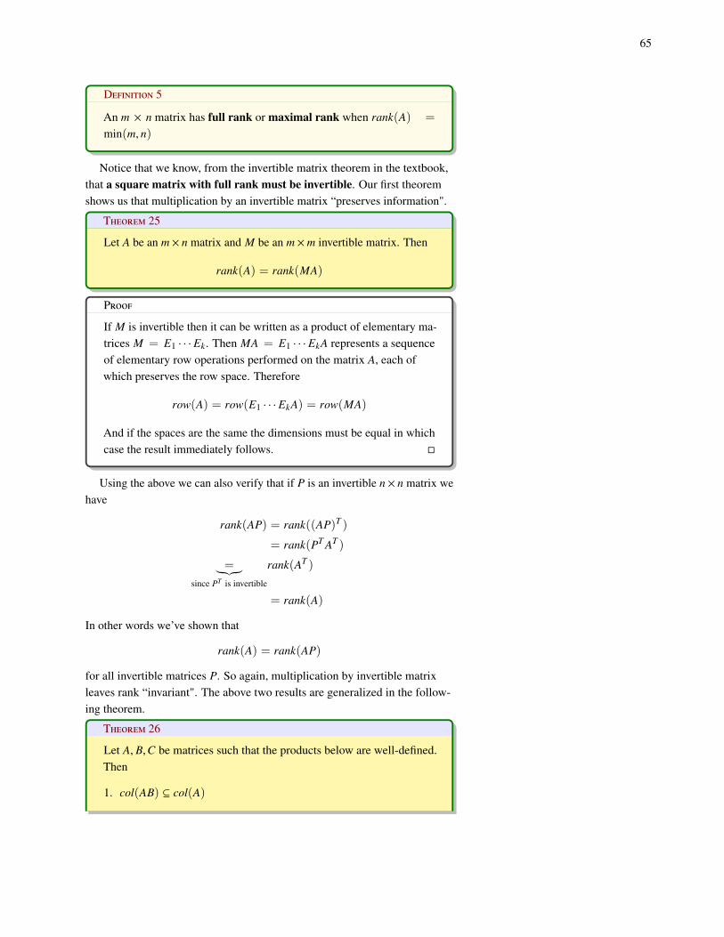
65
Definition 5
An m × n matrix has full rank or maximal rank when rank(A) =
min(m, n)
Notice that we know, from the invertible matrix theorem in the textbook,that a square matrix with full rank must be invertible. Our first theoremshows us that multiplication by an invertible matrix “preserves information".
Theorem 25
Let A be an m × n matrix and M be an m ×m invertible matrix. Then
rank(A) = rank(MA)
Proof
If M is invertible then it can be written as a product of elementary ma-trices M = E1 · · · Ek. Then MA = E1 · · · EkA represents a sequenceof elementary row operations performed on the matrix A, each ofwhich preserves the row space. Therefore
row(A) = row(E1 · · · EkA) = row(MA)
And if the spaces are the same the dimensions must be equal in whichcase the result immediately follows. �
Using the above we can also verify that if P is an invertible n × n matrix wehave
rank(AP) = rank((AP)T )
= rank(PT AT )
=︸︷︷︸since PT is invertible
rank(AT )
= rank(A)
In other words we’ve shown that
rank(A) = rank(AP)
for all invertible matrices P. So again, multiplication by invertible matrixleaves rank “invariant". The above two results are generalized in the follow-ing theorem.
Theorem 26
Let A, B, C be matrices such that the products below are well-defined.Then
1. col(AB) ⊆ col(A)

66
2. row(CA) ⊆ row(A)
In the above ⊆ will simply be = when B or C respectively is invert-ible.
Proof
We only prove the first statement since the proof of the other can beshown to follow by use of transposes. Let B have columns {b j}. Thenthe matrix AB has columns {Ab j}, each term Ab j is a linear combi-nation of the columns of A so therefore we have that the columns ofAB are in the column space of A. In other words col(AB) ⊆ col(A).To prove the case of equality we can appeal to the prior results we’vealready seen. Suppose B is invertible. Then, since col(AB) ⊆ col(A)and rank(AB) = rank(A) if B is invertible we see col(AB), a sub-space of col(A), has the same dimension as col(A). Therefore if B isinvertible then col(AB) = col(A). �
A sometimes useful result is the following inequality.
Theorem 27
If A and B are two matrices whose product is defined then
rank(AB) ≤ min(rank(A), rank(B))
Proof
Since the prior theorem showed us that col(AB) ⊆ col(A) we thenhave that rank(AB) = dim(col(AB)) ≤ dim(col(A)) = rank(A).Similarly we have row(AB) ⊆ row(B) gives that rank(AB) =
dim(row(AB)) ≤ dim(row(B)) = rank(B). The result follows. �
Maximal Rank
In this section, we’re going to look at the cases where the rank of an m × nmatrix A is as large as possible. We’ve already seen that the case of maximalrank occurs when rank(A) = min(m, n). If A were square, then A havingfull rank ensures that Ax = b is always uniquely solvable. Since the nullitycaptures the “size" of the subspace controlling the homogeneous solution itcontrols the “size" of the obstruction to uniqueness if the equation is solvablebut not uniquely solvable. The following theorems describe both possibilitiesfor maximal rank.

67
Theorem 28: Rank = # of Columns
Let A be m × n. The following are equivalent statements.
1. rank(A) = n
2. rows of A span Rn
3. columns of A are independent
4. AT A is invertible
5. There’s an n × m matrix C such that CA = In. (The matrix C iscalled a “left inverse" of A)
6. Ax = 0 has only the trivial solution
Proof
I only prove (3) =⇒ (4) =⇒ (5) leaving the cases(5) =⇒ (6) =⇒ (1) =⇒ (2) =⇒ (3) as an exercise.So, suppose that (3) holds and the columns of A are independent.Then that means that Ax = 0 =⇒ x = 0. So consider
AT Ax = 0 =⇒ xT AT Ax = 0
=⇒ (Ax)T Ax = 0
=⇒ [||Ax||2] = 0
=⇒ ||Ax||2 = 0
=⇒ Ax = 0
=⇒ x = 0
So the square matrix AT A admits only the trivial solution for itsassociated homogeneous problem. By the invertible matrix theoremwe have that AT A must be invertible. Thus (3) =⇒ (4).Next, if (4) holds then AT A is invertible. In that case, setC = (AT A)−1AT . Obviously this choice of C gives the desiredconclusion and so (4) =⇒ (5).
�
The other possibility of full rank is dealt with in the next theorem.
Theorem 29: Rank = # of rows
Let A be m × n. The following are equivalent statements.
1. rank(A) = m
2. columns of A span Rm
3. rows of A are independent

68
4. AAT is invertible
5. There’s an n ×m matrix C such that AC = Im
6. Ax = b is solvable for all b ∈ Rm
Proof
I only prove (3) =⇒ (4) =⇒ (5) =⇒ (6) leaving the cases(6) =⇒ (1) =⇒ (2) =⇒ (3) as an exercise. So, supposethat (3) holds and the rows of A are independent. Then that meansthat the m rows are a collection of m independent vectors inside ofRn. But that means that dim(row(A)) = rank(A) = m. From thiswe see that rank(A) = m, but also since rank(AT ) = rank(A) wehave that rank(AT ) = m as well. In other words, the matrix AT , hasrank equal to its amount of columns. Therefore, our prior theorem,applied to the matrix AT , says that (AT )T AT = AAT is invertible.Thus (3) =⇒ (4). Next, assuming (4) we can set C = AT (AAT )−1
and easily verify that AC = I. So (4) =⇒ (5).Finally, assuming (5) means that there’s a matrix C whose columnsc j, j = 1, ..., m solve Ac j = e j. Then, of course, for b ∈ Rm,b = b1e1 + · · · bmem we have
A(b1c1 + · · · bmcm) = b1Ac1 + · · · bmAcm
= b1e1 + · · · bmem
= b
which means that Ax = b is solvable by setting x = b1c1 + · · · bmcm
so (5) =⇒ (6).�
Exercises
You should be able to do the following.
1. Prove that spans of vectors are always subspaces.
2. True/False: If S 1 and S 2 are subspaces of Rn then so is S 1 ∪ S 2. If true,prove it, otherwise give a counterexample.
3. True/False: If S 1 and S 2 are subspaces of Rn then so is S 1 ∩ S 2. If true,prove it, otherwise give a counterexample.
4. Find E3(
1 14 1
) and E−1(
1 14 1
).5. Find Eλ(In) for all values of λ ∈ R.

69
6. Prove that invertible linear transformations map bases of Rn onto bases ofRn. In other words if A is an invertible n × n matrix, prove that {Av j}
nj=1 is
a basis whenever {v}nj=1 is.
7. Prove that if A ∼ B then row(A) = row(B).
8. Prove that the reduction algorithm applied to Ax = 0 will produce abasis for null(A) whenever null(A) , {0}. Hint: think about reducedrow-echelon form.
9. In the proof of Theorem 1.2, how do I know it’s possible to choose alargest set of linearly independent vectors {v1, ..., vk}?
10. It was claimed that the zero subspace admits no basis. Explain why.
11. Suppose that AB is invertible. Is A? If so prove it. If not, give a coun-terexample.
12. Suppose A, B are n× n matrices. Use rank inequalities to show that if A isnot invertible then AB must be non-invertible as well.
13. Prove that if U, V are subspaces of Rn then U ⊆ V implies dim U ≤dim V .
14. Use a theorem on maximal rank to prove that the polynomial p(x) =
1 + x2 has no real roots.
15. Let A =[2 2 3
]. Find a basis for ker(A) and a basis for ker(AT ).
16. Suppose that A, B are square matrices of the same size and that col(B) ⊆ker A. What can I say about AB?
17. Let A = [ai j] where ai j = i + j for 1 ≤ i, j ≤ n. Determine rank(A).
18. Suppose that A is m × n. Show that ker A = ker(UA) for all invertiblem ×m matrices U. Then also show that dim(ker(A)) = dim(ker(AB)) forall invertible n × n matrices B.
19. Let
A =
1 2 33 2 1
(a) Find a matrix B such that AB = I2 or show that such a B doesn’t exist.
(b) Find a matrix C such that CA = I3 or show that such a C doesn’texist.
20. Let
A =
a 1 a 0 0 00 b 1 b 0 00 0 c 1 c 00 0 0 d 1 d
where a, b, c, d are unspecified real numbers.

70
(a) Prove that rank(A) > 2.
(b) Prove that if a = d = 0 and bc = 1 then rank(A) = 3.
21. Let A be an n × n matrix.
(a) Show that A2 = 0 if and only if col(A) ⊆ ker(A).
(b) Show that A2 = 0 implies rank(A) ≤ n2
(c) Find a matrix A such that col(A) = null(A)
22. Let c , 0 be in Rm and r ∈ Rn and define A = crT
(a) Show that col(A) = span{c} and row(A) = span{r}.
(b) Find dim(ker(A))
(c) Show that ker A = null(r)
23. Prove that if dim S = m then any set of m linearly independent vectors inS must be a basis.
24. Prove that if dim S = m then any set of m spanning vectors in S must bea basis.
25. Prove that the only proper subspaces of R3 are lines through the originand planes through the origin.
26. Prove the remaining equivalent statements in the theorems on full rank(Theorems 9 & 10).
27. Let B be m × n and AB be k × n. Suppose that rank(AB) = rank(B).Show that ker B = ker(AB).
28. Show that, for every n ×m matrix A, the matrix Im + AT A is invertible.
29. Suppose that S ⊂ R8 where dim S = 5. Is there a subspace V ⊆ R8 suchthat dim V = 2 and V ∩ S = {0}. Justify your answer.

The Fundamental Theorem of Linear Algebra
We are going to present a striking result, fundamental to understandinghow the concepts we’ve seen all semester relate to one another. But, equallyimportant, we’re going to see a remarkable picture which illustrates thetheorem.
Contents
Prelude: Orthogonal Complements 72
The Fundamental Theorem of Linear Algebra 73
The Diagrams 75
Decomposition of Rn 75
Decomposition of Rm 76
An application 76
Exercises 79

72
Prelude: Orthogonal Complements
Before we get to the main theorem, a bit on the terminology it uses. We’llbegin with a natural definition.
Definition 6
Let S ⊆ Rn be a subspace. The set S⊥ ⊆ Rn is defined to be the col-lection of all vectors v ∈ Rn orthogonal to S and called the orthogo-nal complement of S in Rn. In other words,
S⊥ = {u ∈ Rn | u · v = 0, v ∈ S }
You should be able to prove that S⊥ is a subspace of Rn (see exercises)The purpose of these notes is to establish a version of the Fundamental
Theorem of Linear Algebra. The result can be thought of as a type ofrepresentation theorem, namely, it tells us something about how vectors areby describing the canonical subspaces of a matrix A in which they live. Tounderstand this we consider the following representation theorem.
Theorem 30
Let v ∈ Rn and let S ⊆ Rn be a subspace. Then there are vectors s ∈S , s⊥ ∈ S⊥ such that
v = s + s⊥
In other words, vectors can be expressed in terms of pieces living inorthogonal spaces.
The above theorem is sometimes expressed in the notation Rn = S ⊕ S⊥
where the notation is called the “direct sum" of S and S⊥.Proof
The proof needs a small fact we saw early in the section on Gram-Schmidt. Here’s the fact: not only does every subspace S of Rn
have a basis, it actually has an orthonormal basis, namely a basis Bconsisting of vectors s j where ||s j|| = 1 holds for all j and si · s j = 0when i , j. How do we know? We’ve already proven that subspacesall have bases. From there all that’s left is to use the Gram-Schmidtalgorithm to turn a given basis into one in which all the vectors aremade orthogonal and of unit length.So S has an orthonormal basis as described. Then set
s = (v · s1)s1 + · · ·+ (v · sdim S )sdim S
which must clearly be an element of S . Then define s⊥ = v − s. It’sobvious that v = s + s⊥ and you can verify that s⊥ ∈ S⊥ giving theresult. �

73
Example 16
Consider the subspace S = span{e1} ⊂ R4. Then S⊥ = {v ∈ R4 | v ·e1 = 0}. A basis for S⊥ is provided by {e2, e3, e4}. Clearly any vectorw ∈ R4 can be written as
w = c1e1 + c2e2 + c3e3 + c4e4 = s + s⊥
as claimed by the theorem.
Where this is going: We’ll soon see that for an m × n matrix A we have(ker A)⊥ = col(AT ). If this is true, then that means (using the notation above)that Rn = ker(A) ⊕ col(AT ). In this case a vector x ∈ Rn can be writtenas x = p + v where Av = 0 and p ∈ row(A) since row(A) = col(AT ).In other words if b ∈ col(A) we can solve Ax = b and since x ∈ Rn =
ker(A) ⊕ col(AT ) we can write x as
x = p + vh
In the above p ∈ row(A) since row(A) = col(AT ). The space of possiblevh’s is dim(ker(A))-dimensional, so the nullity describes the lack of uniquesolvability for the linear system Ax = b.
The Fundamental Theorem of Linear Algebra
We can now get on with proving the main theorem in this course, the cap-stone to our understanding what it means to solve systems of linear equations.
Proposition 1
Suppose A is an m × n matrix. Then
col(AT )⊥ = ker A
Proof
Suppose v ∈ ker A, then Av =
00...0
=
(row1(A)) · v(row2(A)) · v
...(rowm(A)) · v
so v is or-
thogonal to rowi(A) for i = 1, ..., m. Therefore v ∈ (row(A))⊥ =
(col(AT ))⊥, i.e. ker A ⊆ (col(AT ))⊥. As well, if v ∈ (col(AT ))⊥
then, in particular, we must have that v · (rowi(A)) = 0 for i = 1, ..., m.But in this case we’d again have v ∈ ker A. Thus (col(AT ))⊥ ⊆ ker A.Since the sets contain each other they must be equal and we’re done.
�

74
If v ∈ (S⊥)⊥ then clearly v · s⊥ = 0 for all s⊥ ∈ S⊥. If {s1, ..., sdim S } isan orthonormal basis for S and {s⊥1 , ..., s⊥dim S⊥ } is an orthonormal basis for S⊥
we can write out (from the expansion formula we saw earlier)
v = (v · s1)s1 + · · ·+ (v · sdim S )sdim S + (v · s⊥1 )s⊥1 + · · ·+ (v · s⊥dim S⊥)s
⊥dim S⊥
= (v · s1)s1 + · · ·+ (v · · · sdim S )sdim S ∈ S
So (S⊥)⊥ ⊆ S . As well, clearly for s ∈ S we have s ∈ (S⊥)⊥ since s · s⊥ = 0must be true for all s⊥ ∈ S⊥. Thus, S ⊆ (S⊥)⊥. From these facts it followsthat
S = (S⊥)⊥
must hold for all subspaces S ⊆ Rn. (Make sure you can verify this state-ment). Applying this general fact to the previous theorem we immediately getthe following.
Theorem 31: Fundamental Theorem of Linear Algebra
Suppose A is an m × n matrix. Then
col(AT ) = (ker A)⊥
So thatRn = ker(A) ⊕ col(AT )
gives an orthogonal decomposition of Rn into the null space andthe row space of matrix A. Therefore, for b ∈ col(A) we have thatAx = b is solved by
x = p + vh
for p ∈ row(A) a particular solution, Ap = b, and vh ∈ ker A ageneric vector in ker A.
Example 17
Consider the matrix A =
1 0 7 60 1 5 20 0 0 0
. The fundamental theorem,
applied to AT , tells us that Rm = ker(AT ) ⊕ col(A), which in this casegives R3 = ker(AT ) ⊕ col(A). Let’s see if this holds.Since the matrix is in reduced form, we know that a basis for col(A)
is given by the pivot columns, namely {
100
,
010
}. Next, look at
ker(AT ). Since AT =
1 0 00 1 07 5 06 2 0
we use row reduction to find a basis

75
for the null space. Namely, AT ∼
1 0 00 1 00 0 00 0 0
and therefore, a basis for
ker(AT ) is given by {
001
}. Notice that, indeed, ker(AT ) = (col(A))⊥
and that R3 = ker(AT ) ⊕ col(A) as the theorem dictates.
The Diagrams
The content of this theorem, the fundamental theorem of linear algebra, isencapsulated in the following figure. If a picture is worth a thousand words,these figures are worth at least several hours’ thought. The figures shouldbe thought of as a visualization of the effect of the linear transformation TA,induced by m × n matrix A with rank r.
Decomposition of Rn
Here we consider the orthogonal decomposition described by the fundamen-tal theorem of the domain of TA, namely Rn = ker A ⊕ col(AT ).
Figure 5: Solving Ax = b for an m × nmatrix with rank(A) = r. The subspaceson both sides meet at right angles. Noticethat the subspaces appearing on the leftcorrespond to their “dual subspaces" forcorresponding transpose of the matrix Aappearing on the right hand side.
Notice this picture has all the major players we’ve seen in this course:there are vectors, subspaces, dimensions, and they are all playing a role in the

76
way we conceptualize solving a linear system of equations. Moreover, notethe duality in the picture: the subspaces on the right-hand side, those living inRm, are the corresponding subspaces appearing on the left-hand side for thetranspose of A rather than A (e.g. col(A) appearing on the upper right is justrow(AT ) whereas we see row(A) on the upper left-hand side). The subspacesmeet at right angles because they’re orthogonal complements of each otherand the intersection of the spaces is the zero subspace of the respectiveambient space (Rn or Rm). Try to visualize how the picture changes as welook at limiting values of possible rank for A. Namely, how would this abovechange in the case where rank(A) = n say? Or m? Or if A is square andinvertible? If A is symmetric? Etc.
Decomposition of Rm
Next, we consider a nice application of the orthogonal decomposition of thecodomain of the transformation TA described by the fundamental theorem oflinear algebra, namely Rm = ker AT ⊕ col(A).
Figure 6: Finding the best x when Ax = bisn’t solvable since b < col(A) for an m × nmatrix with rank(A) = r. The subspaceson both sides meet at right angles. Sinceb < col(A) the equation Ax = b isn’tsolvable. But the orthogonal decompositionof Rm allows a natural approach to findingthe “best" x.
An application
We’re going to expand on the last picture a bit. Consider the followingsituation. We’ve collected m output numbers y1, ..., ym from a measuringdevice at various times labeled t1, t2, ..., tm. In other words, we have collecteddata of the form (ti, yi) for i = 1, ..., m. The values yi could be the reportedvaluation on a stock we are interested in purchasing, say, where the “device"is a computer ticker displaying the values. The values yi could be the medianselling price of a home in a given neighbourhood at a given time ti, say. The“device" in this instance, might again be an annual financial report or internal

77
publication. The point is, the situation I’ve described is quite general. Maybethe data we’ve collected looks something like the following
Figure 7: A plot of data points (ti, yi) forvarious t values.
It would be of obvious financial value to be able to use the data we’vegathered to be able to predict new data at times in the future. This would bedoable if, say, we had a model for how the data were produced, namely if wehad a function f : R→ R for which
yi = f (ti), i = 1, ..., m
Simplicity being preferable to complexity in modelling, the easiest thingto consider as a first approximation would be a linear model. Namely, weassume f takes the form f (w) = mw + b for fixed numbers m, b. In that casewe’re searching for a model to be able to use for predictive purposes whichtakes the form
yi = ati + b i = 1, ..., m (0.0.5)
The problem is that you can see from the figure above that the data pointsclearly cannot live on a line. On the other hand, they aren’t that far off somaybe it’s not hopeless either. Since, as modellers, we’re allowed to choosethe parameters a, b as we like, we can view them as unknowns in the problemand try to use the data set to determine the best possible choice.
We rewrite equation (0.0.5) as the matrix equation
1 t11 t21 t3...
...1 tm
A
ba
x
=
y1
y2
y3...
ym
b
(0.0.6)

78
Since we’ve already noticed that the points (ti, yi) don’t live on a line weknow that, in the above, we have b < col(A), so there’s no chance of actuallysolving the above matrix equation to actually determine the parameters a, b.But a glance at Figure 2, together with the discussion preceding it, indicatesthat we shouldn’t give up. Namely, instead of solving Ax = b which weknow we cannot, we find the vector y ∈ col(A) which is as close as possibleto b. As before, this vector must satisfy AT (y − b) = 0 which means we wantto solve
AT Ax = AT b
Then again, in this particular case, since t1 < t2 < · · · < tm we have thatrank(A) = 2. Our theorem on maximal rank guarantees then that AT A mustbe invertible. Therefore, we have found an optimal solution
x = (AT A)−1AT b
In other words, the parameters m, b which provide us with a “best linearfit" for the data set are
ba = (
1 1 · · · 1t1 t2 · · · tm
1 t11 t21 t3...
...1 tm
)−1
1 1 · · · 1t1 t2 · · · tm
y1
y2
y3...
ym
We can clean this up a little by defining 1 =
[1 1 · · · 1
]Tand t =[
t1 t2 · · · tm]T
. This allows us to rewrite the above as
ba = (
1 1 · · · 1t1 t2 · · · tm
1 t11 t21 t3...
...1 tm
)−1
1 1 · · · 1t1 t2 · · · tm
y1
y2
y3...
ym
=
m 1 · t1 · t ||t||2
−1 1 1 · · · 1t1 t2 · · · tm
y1
y2
y3...
ym
=
1m||t||2 − (1 · t)
||t||2 −1 · t−1 · t m
1 · bt · b
So that b = (
||t||21−(1·t)tm||t||2−(1·t) ) · b and a = (
mt−(1·t)1m||t||2−(1·t) ) · b give the best choice of
parameters for fitting the data to a line.

79
Figure 8: A plot of data points (ti, yi)together with the line y = ax + b where a, bare the best possible parameters. Notice thatwhile the points don’t fall on the line, theyare not far off.
Exercises
You should be able to do the following.
1. Calculate the orthogonal complements of the improper subspaces of Rn.
2. Let v ∈ R3 be a nonzero vector. Describe (span{v})⊥.
3. Prove that S⊥ is a subspace of Rn whenever S is.
4. Prove that for S ⊆ Rn a subspace we have dim S + dim S⊥ = n.
5. If S , W are subspaces of Rn show that S ⊆ W =⇒ W⊥ ⊆ S⊥
6. Let S = {x ∈ R4 | x1 + x2 + x3 + x4 = 0}. Prove that S is a subspace andfind a basis for S⊥.
7. Prove that every m × n matrix A defines a linear transformation fromrow(A) onto col(A), i.e.
TA : row(A)→ col(A)
8. Consider A, an m × n matrix and b ∈ Rm. Consider the following claim28: 28 A variation of this strange-sounding claimis very important in numerous applicationsincluding, very importantly, in differentialequations.
One and only one of the following systems is solvable
(a) Ax = b
(b) AT y = 0 with yT b , 0
Prove that the above options cannot BOTH hold. In other words, if one ofthe above holds the other one mustn’t.

80


![Introduction - math.toronto.edu · 2 VANYA TELPUKHOVSKIY from[28]thatalongthisTeichmüllergeodesictheboundarycurvesofsubsurfaces i(Y) definedinSection3.1willbe shrinking. Unlikethat,asourresultassures](https://static.fdocuments.net/doc/165x107/5d2da5dc88c99309368c6679/introduction-math-2-vanya-telpukhovskiy-from28thatalongthisteichmuellergeodesictheboundarycurvesofsubsurfaces.jpg)