LINEAR ALGEBRA—A GEOMETRIC

INTRODUCTION I

J. B. CooperJohannes Kepler Universitat Linz

Contents

1 LINEAR EQUATIONS AND MATRIX THEORY 41.1 Systems of linear equations, Gaußian elimination . . . . . . . 41.2 Matrices and their arithmetic . . . . . . . . . . . . . . . . . . 91.3 Matrix multiplication, Gaußian elimination

and hermitian forms . . . . . . . . . . . . . . . . . . . . . . . 291.4 The rank of a matrix . . . . . . . . . . . . . . . . . . . . . . . 391.5 Matrix equivalence . . . . . . . . . . . . . . . . . . . . . . . . 451.6 Block matrices . . . . . . . . . . . . . . . . . . . . . . . . . . 501.7 Generalised inverses . . . . . . . . . . . . . . . . . . . . . . . . 551.8 Circulants, Vandermonde matrices . . . . . . . . . . . . . . . . 58

2 ANALYTIC GEOMETRY IN 2 and 3 DIMENSIONS 612.1 Basic geometry in the plane . . . . . . . . . . . . . . . . . . . 612.2 Angle and length . . . . . . . . . . . . . . . . . . . . . . . . . 672.3 Three Propositions of Euclidean geometry . . . . . . . . . . . 712.4 Affine transformations . . . . . . . . . . . . . . . . . . . . . . 752.5 Isometries and their classification . . . . . . . . . . . . . . . . 782.6 Conic sections . . . . . . . . . . . . . . . . . . . . . . . . . . . 892.7 Three dimensional space . . . . . . . . . . . . . . . . . . . . . 942.8 Vector products, triple products, 3× 3 determinants . . . . . . 992.9 Covariant and contravariant vectors . . . . . . . . . . . . . . . 1042.10 Isometries of R3 . . . . . . . . . . . . . . . . . . . . . . . . . . 107

3 VECTOR SPACES 1133.1 The axiomatic definition, linear dependence

and linear combinations . . . . . . . . . . . . . . . . . . . . . 1133.2 Bases (Steinitz’ Lemma) . . . . . . . . . . . . . . . . . . . . . 117

1

3.3 Complementary subspaces . . . . . . . . . . . . . . . . . . . . 1223.4 Isomorphisms, transfer matrices . . . . . . . . . . . . . . . . . 1243.5 Affine spaces . . . . . . . . . . . . . . . . . . . . . . . . . . . . 127

4 LINEAR MAPPINGS 1324.1 Definitions and examples . . . . . . . . . . . . . . . . . . . . 1324.2 Linear mappings and matrices . . . . . . . . . . . . . . . . . 1344.3 Projections and splittings . . . . . . . . . . . . . . . . . . . . 1394.4 Generalised inverses of linear mappings . . . . . . . . . . . . . 1434.5 Norms and convergence in vector spaces . . . . . . . . . . . . 144

2

Preface In these notes we have tried to present the theory of matrices,vector spaces and linear operators in a form which preserves a balance be-tween an approach which is too abstract and one which is merely compu-tational. The typical linear algebra course in the early sixties tended to bevery computational in nature, with emphasis on the calculation of variouscanonical forms, culminating in a treatment of the Jordan form without men-tioning the geometrical background of the constructions. More recently, suchcourses have tended to be more conceptual in form beginning with abstractvector spaces (or even modules over rings!) and developing the theory inthe Bourbaki style. Of course, the advantage of such an approach is that itprovides easy access and a very efficient approach to a great body of classicalmathematics. Unfortunately, this was not exploited in many such courses,leaving the abstract theory a torso, deprived of any useful sense for manystudents. The present course is an attempt to combine the advantages ofboth approaches. It begins with the theory of linear equations. The methodof Gaußian elimination is explained and, with this material as motivation,matrices and their arithmetic are introduced. The method of solution and itsconsequences are re-interpreted in terms of this arithmetic. This is followedby a chapter on analytic geometry in two and three dimensions. Two bytwo matrices are interpreted as geometric transformations and it is shownhow the arithmetic of matrices can be used to obtain significant geometricalresults. The material of these first two chapters and this dual interpretationof matrices provides the basis for a meaningful transition to the axiomatictheory of vector spaces and linear mappings.

After this introductory material, I have felt free to use increasingly higherlevels of abstraction in the remainder of the book which deals with determi-nants, the eigenvalue problem, diagonalisation and the Jordan form, spectraltheory and multilinear algebra. I have also included a brief introduction tothe complex numbers. The book contains several topics which are not usu-ally covered in introductory text books—of which we mentioned generalisedinverses (including Moore-Penrose inverses), singular values and the classi-fication of the isometries in R2 and R3. It is also accompanied by threefurther volumes, one on elementary geometry (based on affine transforma-tions) one containing a further set of exercises and one an introduction toabstract algebra and number theory.

I have taken pains to include a large number of worked examples and ex-ercises in the text. The latter are of two types. Each set begins with routinecomputational exercises to allow the reader to familiarise himself with theconcepts and proofs just covered. These are followed by more theoretical ex-ercises which are intended to serve the dual purpose of providing the studentwith more challenging problems and of introducing him to the rich array of

3

mathematics which has been made accessible by the theory developed.

1 LINEAR EQUATIONS ANDMATRIX THE-

ORY

1.1 Systems of linear equations, Gaußian elimination

The subject of our first chapter is the classical theory of linear equations andmatrices. We begin with the elementary treatment of systems of linear equa-tions. Before attempting to derive a general theory, we consider a concreteexample:

Examples. Solve the system

3x − y = 6 (1)x + 3y − 2z = 1 (2)2x + 2y + 2z = 2. (3)

We use the familiar method of successively eliminating the variables: re-placing (2) by 3 · (2)− (1) and (3) by 3 · (3)− 2(1) we get the system:

3x − y = 6 (4)10y − 6z = −3 (5)8y + 6z = −6. (6)

We now proceed to eliminate y in the same manner and so reduce to thesystem:

3x − y = 6 (7)10y − 6z = −3 (8)

54z = −18 (9)

and this system can be solved “backwards” i.e. by first calculating z fromthe final equation, then y from (8) and finally x. This gives the solution

z = −1

3y = −1

2x =

11

6.

(Of course, it would have been more sensible to use (2) in the original systemto eliminate x from (1) and (3). We have deliberately chosen this more me-chanical course since the general method we shall proceed to develop cannottake such special features of a concrete system into account).

In order to treat general equations we introduce a more efficient notation:

a11x1 + . . . + a1nxn = y1...

...am1x1 + . . . + amnxn = ym

4

is the general system of m equations in n unknowns. The aij are the co-efficients and the problem is to determine the values of the x for giveny1, . . . , ym.

In this context we can describe the method of solution used above asfollows. (For simplicity, we assume that m = n). We begin by subtractingsuitable multiples of the first equation from the later ones in such a way thatthe coefficients of x1 in these equations vanish. We thus obtain a system ofthe form

b11x1 + b12x2 + . . . + b1nxn = z1b22x2 + . . . + b2nxn = z2

......

bn1x2 + . . . + bnnxn = zn.

(with new coefficients and a new right hand side). Ignoring the first equation,we now have a reduced system of (n−1) equations in (n−1) unknowns and,proceeding in the same way with this system, then with the resulting systemof (n− 2) equations and so on, we finally arrive at one of the form:

d11x1 + d12x2 + . . . + d1nxn = w1

d22x2 + . . . + d2nxn = w2...

...dnnxn = wn

which we can solve simply by calculating the value of xn from the last equa-tion, substituting this in the second last equation and so working backwardsto x1.

This all sounds very simple but, unfortunately, reality is rather morecomplicated. If we call the coefficient of xi in the i-th equation after (i− 1)steps in the above procedure the i-th pivot element, then the applicabilityof our method depends on the fact that the i-th pivot is non-zero. If it iszero, then two things can happen.Case 1: the coefficient of xi in a later equation (say the j-th one) is non-zero.Then we simply exchange the i-th and j-th equations and proceed as before.Case 2: the coefficients of xi in the i-th and all following equations vanish.In this case, it may happen that the system has no solution.

Examples. Consider the systems

x + y + 2z = −2 2x + 3y − z = 13x + 3y − 4z = 6 6x + y + z = 32x − y + 6z = −1 4x + 2y = −1.

5

If we apply the above method to the first system we get successively

x + y + 2z = −2−10z = 12

−3y + 2z = 3

i.e.x + y + 2z = −2

−3y + 2z = 3−10z = 12

and this is solvable.In the second case, we get:

2x + 3y − z = 1−8y + 4z = 0−4y + 2z = −3.

At this stage we see at a glance that the system is not solvable (the last twoequations are incompatible) and indeed the next step leads to the system

2x + 3y − z = 1−8y + 4z = 0

0 = 6

and the third pivot vanishes. Note that the vanishing of a pivot element doesnot automatically imply the non-solvability of the equation. For example, ifthe right hand side of our original equation had been

486

then it would indeed have been solvable as the reader can verify for himself.Hence we see that if a pivot element is zero in the non-trivial manner of

case 2 above, then we require a more subtle analysis to decide the solvabilityor non-solvability of the system. This will be the main concern of this Chapterwhereby the method and result will be repeatedly employed in later ones. Auseful tool will be the so-called matrix formalism which we introduce inthe next section.

Examples. Solve the following systems (if possible):

2x + 4y + z = 1 x + 5y + 2z = 93x + 5y = 1 x + y + 7z = 65x + 13y + 7z = 5 −3y + 4z = −2.

6

Solution: In the first case we subtract 7 times the first equation from thethird one and get

−9x− 15y = −2

which is incompatible with the second equation.In the second case, we subtract the 2nd one from the first one and get

4y − 5z = 3.

This, together with the third equation, gives y = 2, z = 1. Hence x = −3and this solution is unique.

Exercises: 1) Solve the following systems (if possible):

y1 + y2 = ay2 + y3 = b

y3 + y4 = cy1 + y4 = d.

2x + y + 2z − w = 06x + 8y + 12z − 13w = −2110x + 2y + 2z + 3w = 21−4x + z − 3w = −13.

2) Which of the following two systems of equations has a solution?

2x + 4y + z = 1 x + 5y + 2z = 93x + 5y = 1 x + y + 7z = 65x + 13y + 7z = 5 − 3y + 4z = −2.

3) For which values of a, b, c does the system

x + y + z = 1ax + by + cz = 1a2x + b2y + c2z = 1.

have a solution? In case it does, calculate it explicitly.4) For which values of a does the system

x + y − z = 12x + 3y + az = 3x + ay + 3z = 2

7

have a unique solution? 5) For which values of a, b, c and d is the equation

2x + y + 2z = ax + 2y + z = b−x − y = c

y = d

solvable?6) Show that the system

ax+ by = ecx+ dy = f

is solvable for every value of e and f if and only if ad− bc 6= 0. The solutionis then unique and is given by the formula

x =ed− bf

ad− bcy =

af − ce

ad− bc.

7) Find suitable constants a, b, c, . . . so that

• 1 + 2 + · · ·+ n = an2 + bn + c;

• 1 + 3 + · · ·+ (2n− 1) = an2 + bn + c;

• 12 + 22 + · · ·+ n2 = an3 + bn2 + cn+ d.

(Of course, the constants may be different in each case).

8

1.2 Matrices and their arithmetic

Consider again our original system

3x − y + 0.z = 6x + 3y − 2z = 12x + 2y + 2z = 2.

The information contained in these equations can be reduced to two schemesof numbers—the coefficients of the unknowns—which can be written thus:the coefficients of the left hand side

3 −1 01 3 −22 2 2

and the right hand side

012

.

For the general system

a11x1 + . . . + a1nxn = y1...

...am1x1 + . . . + amnxn = ym

the corresponding schemes are:

a11 . . . a1n...

...am1 . . . amn

resp.

y1...ym

.

We call such an array

a11 . . . a1n...

...am1 . . . amn

an m×nmatrix. m is the number of rows, n the number of columns of thematrix which can be written in shortened form as [aij ]

m,ni=1,j=1 or simply [aij ]

9

when it is not necessary to specify m and n. We use capital letters A,B,C,. . .to denote matrices: thus A = [aij ] means that the (i, j)-th element (i.e. theelement in the i-th row and j-th column) of A is aij .

Similarly,

y1...ym

is an m× 1 matrix. Such matrices are called column matrices for obviousreasons. Thus the j-th column of A = [aij ] is the m× 1 matrix

a1j...amj

.

Similarly, the i-th row is the 1× n row matrix

[

ai1 . . . ain]

.

If Ai (resp. Bj) is the i-th row (resp. j-th column) of A it is sometimesconvenient to write A in the forms:

A1...Am

or[

B1 . . . Bn

]

.

Examples.[

6 −3 71 1 −1

]

is a 2× 3 matrix. Its second row is

[

1 1 −1]

and its third column is[

7−1

]

.

The (2, 3)-rd element is −1.We list some important special matrices resp. types of matrices. Note

the systems of equations to which they correspond.

10

1) the m× n zero matrix

0 . . . 0...

...0 . . . 0

(i.e. the matrix with all entries zero). This corresponds to the system

0 · x1 + . . . + 0 · xn = y1...

...0 · x1 + . . . + 0 · xn = ym

which is solvable only when the right hand side vanishes. Then any n-tuple(x1, . . . , xn) is a solution. We denote this matrix by 0m,n or, less pedantically,by 0.2) the n× n matrix

1 0 . . . 00 1 . . . 0...

...0 . . . 1

which has one’s in the main diagonal and zeros elsewhere. This matrix iscalled the unit matrix, denoted by In or simply by I. It corresponds to thesystem

x1 + 0· x2 + . . . + 0 · xn = y1...

...xn = yn

which always has a unique solution (in fact, it is its own solution!).It is customary to introduce the so-calledKronecker δ-symbol δij where

δij = 1 if i = j, δij = 0 otherwise. Then we can describe I succinctly by theformula I = [δij ].3) diagonal matrices: these are square matrices (i.e. n×n matrices for somen) of the form

λ1 0 . . . 00 λ2 . . . 0...

...0 0 . . . λn

i.e. matrices whose only non-zero elements are in the main diagonal. We usethe shorthand diag (λ1, . . . , λn) to denote this matrix. It corresponds to the

11

system:

λ1 . . . = y1...

...λnxn = yn.

If all of the λi are non-zero, then this always has a unique solution. If any ofthem vanish, then it is solvable only for those right hand sides which vanishat each equation where the λi vanishes and the solution is not unique sincethe corresponding xi can be chosen arbitrarily.4) (upper) triangular matrices. These are square matrices A = [aij ] for whichaij = 0 if i > j i.e. they have the form

a11 a12 . . . a1n0 a22 . . . a2n...

...0 0 . . . ann

.

Lower triangular matrices are defined similarly, the condition being thataij = 0 if i < j.

Note that in the case of n equations in n unknowns, the elimination pro-cess described above is intended to replace a general system by one with atriangular matrix, for the very good reason that the solution of such an equa-tion (if it exists) can be read off directly, starting with the last equation. Onceagain it is precisely the condition that the diagonal elements a11, . . . , ann donot vanish which is required to ensure uniqueness and existence of solutionsfor systems with triangular matrices.

Returning to the topic of linear equations, we can now streamline ournotation by writing the general equation in the form

AX = Y

where A is the m× n matrix [aij ] and X is

x1...xn

and Y

y1...ym

12

. Up to this point, our introduction of the matrix formalism has broughtnothing more than a simplification of the notation. We shall now introducean “arithmetic” for matrices which is closely connected with properties ofthe corresponding systems of equations and which will provide the machinerythat we require for a theory of such systems. More precisely, we shall equipcertain sets of matrices with an addition and a multiplication as follows:

Addition: We add two m × n matrices A and B simply by adding theirrespective components. The result is denoted by A+B. In symbols:

[aij ] + [bij ] = [aij + bij ].

For example:

6 32 −11 −1

+

7 9−2 20 3

=

13 120 11 2

.

Note that we only add matrices of the same type (i.e. with the same numbersof rows and columns). Thus the sum of a 3 × 1 and a 1 × 2 matrix is notdefined.

Addition of matrices possesses many properties which are reminiscent ofthose of addition of real numbers e.g.

• A +B = B + A (commutativity);

• A + (B + C) = (A+B) + C (associativity);

• A = 0 = 0 + A = A;

• A + (−A) = 0 where −A is the matrix [−aij ].In future we shall write A−B for the matrix A+ (−B).

These properties are verified by noting that the corresponding equationshold element for element. For example, A+B = B + A since

A +B = [aij + bij ] = [bij + aij] = B + A.

Another operation which will be useful is that of scalar multiplicationi.e. the multiplication of each element of A by a given λ in R. The result isdenoted by λA (i.e. λA = [λaij ]).

For example:

3

[

1 6 1−1 2 −1

]

=

[

3 18 3−3 6 −3

]

.

This multiplication has the following properties:

13

• λ(A+B) = λA+ λB;

• (λµ)A = λ(µA);

• (λ+ µ)A = λA+ µA;

• 1 · A = A, (−1) · A = −A.We now consider multiplication of matrices. Here it is not quite so cleara priori how the product of two matrices should be defined and we beginwith some remarks which may help to motivate the formal definition. If wewrite our general system of equations in the form AX = Y as above, then itis natural to define the product of an m × n matrix A = [aij] and an n × 1matrix X as above to be the m× 1 matrix

a11x1+ · · ·+ a1nxn...

...am1x1+ · · ·+ amnxn

.

Then if B is the n× p matrix of the form

0 0 . . . 0 b1k 0 . . . 0...

......

0 0 . . . 0 bmk 0 . . . 0

(where the column of b’s is in the k-th column), it is natural to define AB tobe the m× p matrix

0 0 . . . 0 a11b1k + · · ·+ a1nbnk 0 . . . 0...

......

0 0 . . . 0 am1b1k + · · ·+ amnbnk 0 . . . 0

.

Now if we assume that multiplication obeys the usual rules of arithmeticwe can calculate the general product AB where B = [bjk] as follows: We writeB as a sum of p matrices of the above form i.e. each with one non-vanishingcolumn. We then multiply out as if the usual distributive law holds.

We illustrate this with the example:[

−1 6−2 1

] [

1 −1 21 1 3

]

.

We express the product as[

−1 6−2 1

]([

1 0 01 0 0

]

+

[

0 −1 00 1 0

]

+

[

0 0 20 0 3

])

.

14

If we multiply out each term using the above rule and simplify, we obtainthe matrix

[

5 7 16−1 3 −1

]

.

This leads naturally to the following definition: if A = [aij ] is an m × nmatrix and B = [bjk] an n× p matrix, then their product AB is defined tobe the m× p matrix C = [cik] where

cik =n∑

j=1

aijbjk.

That is, the (i, k)-th element of C is obtained by running along the i-th rowof A and the k-th column of B, multiplying successively the correspondingelements and then taking the sum. From this description it is clear that theproduct AB is only defined when the number of columns of A equals thenumber of rows of B. In particular, the expression A · A (which we shortento A2) is defined only when m = n i.e. when A is a square matrix. Then wecan define higher powers A3, A4, . . . , Ak, . . . of A in the obvious way.

Before discussing further properties of matrices, we illustrate the defini-tion of multiplication with a simple example:

Examples. Calculate the products

[

cos θ − sin θsin θ cos θ

]

[

cosφ − sin φsinφ cosφ

]

resp.[

cos θ sin θsin θ − cos θ

]

[

cosφ sin φsin φ − cosφ

]

.

The product of the first two matrices is

[

cos θ cosφ− sin θ sinφ − cos θ sinφ− sin θ cosφsin θ cosφ+ cos θ sinφ − sin θ sinφ+ cos θ cosφ

]

which is equal to

[

cos(θ + φ) − sin(θ + φ)sin(θ + φ) cos(θ + φ)

]

.

15

Similarly,[

cos θ sin θsin θ − cos θ

] [

cos φ sinφsinφ − cos φ

]

=

[

cos(θ − φ) − sin(θ − φ)sin(θ − φ) cos(θ − φ)

]

.

(We shall give a geometric interpretation of these formulae in the nextchapter).

This definition of multiplication can also be motivated by the followingconsiderations. Suppose that we have two systems:

BX = Y and AY = Z.

where the unknowns in the second equation are the right hand side of thefirst. Then eliminating Y from these equations leads to the equation CX = Zwhere C = AB is the product defined above as a little arithmetic shows.

Example Consider the systems

3x + 6y + 4z + 2w = ax + 7y + 8z + 9w = b

−4x − y + 2z + 3w = c

resp.

u = x2u + 4v = y6u − v = z2u + v = w.

Substituting we get the system

3u + 6(2u+ 4v) + 4(6u− v) + 2(2u+ v) = au + 7(2u+ 4v) + 8(6u− v) + 9(2u+ v) = b

−4u − (2u+ 4v) + 2(6u− v) + 3(2u+ v) = c.

with matrix

43 2281 2912 −3

=

3 6 4 21 7 8 9−4 −1 2 3

1 02 46 −12 1

.

We now collect some simple properties of matrix multiplication:1) matrix multiplication is associative i.e. (AB)C = A(BC). (Here, aselsewhere, we tacitly assume, when we write such a formula, that A, B andC satisfy the conditions necessary to ensure that all products which appearare defined. In this case, this means that A is of type m×n, B of type n× pand C of type p× r for suitable m,n, p and r).

Since the above equation is not quite so obvious as those encountered sofar, we bring the proof.

16

Proof. Put A = [aij ], B = [bjk] and C = [ckl]. Then

AB =

[

n∑

j=1

aijbjk

]

ik

and

(AB)C =

[

p∑

k=1

(

n∑

j=1

aijbjk

)

ckl

]

il

.

Similarly

A(BC) =

[

n∑

j=1

aij

(

p∑

k=1

bjkckl

)]

il

.

Hence we must show that

p∑

k=1

(

n∑

j=1

aijbjkckl

)

=

n∑

j=1

(

p∑

k=1

aijbjkckl

)

.

This follows from the general fact that if [djk] is an n× p matrix, then

p∑

k=1

(

n∑

j=1

djk

)

=

n∑

j=1

(

p∑

k=1

djk

)

.

The above relation is clear. We are simply summing all elements of thematrix in two ways—as the sum of the row sums respectively as the sum ofthe column sums. In our example, we put djk = aijbjkckl with i and l fixed.2) multiplication is distributive over addition i.e.

A(B + C) = AB + AC (A +B)C = AC +BC.

One negative property which has important repercussions is:3) multiplication is not commutative i.e. we do not have the equation AB =BA in general. For suppose that A is an m×n matrix and B an n×p matrix.Then if p 6= m, BA is not even defined. If p = m but m 6= n, then AB is anm×m matrix while BA is n×n so they are certainly not equal. This leavesthe only interesting case as the one where m = n = p i.e. where A and Bare square. Even in this case it can (and usually does) happen that AB andBA are distinct. Thus

[

1 10 0

] [

1 01 1

]

=

[

2 10 0

]

17

while[

1 01 1

] [

1 10 0

]

=

[

1 11 1

]

.

4) In is a unit for multiplication: more precisely, if A is an m × n matrix,then

A · In = A = Im · A.One question which plays a central role in the theory of matrices is that

of the invertibility of a matrix. We say that an n×n matrix A is invertibleif there is an n × n matrix B so that AB = BA = I. Note that if we canfind such a B we can reduce the question of solving the equation AX = Yto one of matrix multiplication since X = BY is then a solution. (ForAX = A(BY ) = (AB)Y = I · Y = Y ). We shall examine the relationshipbetween invertibility of A and solvability of the equation AX = Y in moredetail later. In the meantime we continue our remarks on inverses. We notethat there is at most one B with the property that AB = BA = I. For ifAC = CA = I, then

B = B · I = B(AC) = (BA)C = I · C = C.

Hence if A is invertible, we can refer to the inverse of A and denote it byA−1.

Of course, not every n × n matrix is invertible (otherwise every systemof equations would be solvable). The following are simple examples of non-invertible 2× 2 matrices:

[

0 00 0

] [

0 10 0

] [

1 11 1

]

as can easily be checked by direct calculation since the product of thesematrices by a typical 2× 2 matrix

[

b11 b12b21 b22

]

on the right produces the results:

[

0 00 0

] [

b21 b220 0

] [

b11 + b21 b12 + b22b11 + b21 b21 + b22

]

and no choice of the b’s will give the unit matrix.In general, it doesn’t make sense to talk of an inverse for a non-square

matrix A but the concept of a left inverse B i.e. an n × m matrix so

18

that BA = In is meaningful—as is that of a right inverse which is definedanalogously. Note that the argument used above to show that a matrix hasa unique inverse shows that if an n × n matrix A has a right inverse anda left one, then they are automatically equal and so provide an inverse forA. (Later we shall see that if a square matrix has a left or right inverse,then this is automatically an inverse). The same argument also shows thata non-square matrix cannot have both a left and a right inverse.

We now investigate in more detail the connection between the existenceof inverses and the solvability of systems of equations.

Proposition 1 Let A be an m × n matrix and suppose that the equationsAX = Ek are solvable for k = 1, . . . , m where Ek is the k-th column vectorof Im (i.e. the vector with 0’s everywhere except for a 1 in the k-th row).Then A has a right inverse.

Proof. We let the n×1 column vector Xk be a solution of AX = Ek. ThenB = [X1 . . .Xm] is a right inverse for A since

A[X1 . . .Xm] = [AX1 . . . AXm] = [E1 . . . Em].

Of course if A has a right inverse B then the equation AX = Y alwayshas a solution, namely the vector X = BY . We can summarise the situationas follows:

Proposition 2 A has a right inverse if and only if the system AX = Y issolvable for any choice of the right hand side Y .

We illustrate this result by considering some special matrices whose rightinverses (and hence inverses by the above remark since the matrices of ourexamples are square) can be calculated with relative ease:1) the diagonal matrix A = diag (λ1, . . . , λn). Clearly this matrix has a rightinverse if and only if each λi is non-zero and then its right inverse is thediagonal matrix diag (λ−1

1 , . . . , λ−1n ).

2) n× n matrices of the form

λ 1 0 . . . 00 λ 1 . . . 0...

...0 0 0 . . . λ

.

As we shall see later, these play an important role in matrix theory and so weshall denote the above matrix by Jn(λ). The k-th column of its right inverse

19

is the solution of the equation

λx1 + x2+ . . . = 0...

...λxk + xk+1+ . . . = 1

......

λxn = 0

and this is easily seen to be the vector

(−1)k−1λ−k

...1λ

0...0

(where the term1

λis in the k-th row) provided that λ is non-zero.

Hence the (right) inverse of Jn(λ) has the form

1λ

− 1λ2 . . . (−1)n−1

λn

0 1λ

. . ....

...0 0 0 . . . 1

λ

.

3) the above two examples are triangular matrices. By considering the cor-responding system of equations for the general triangular matrix

a11 a12 . . . a1n0 a22 . . . a2n...

...0 0 0 . . . ann

one sees that it has a (right) inverse if and only if the diagonal elements arenon-zero.

We now continue with our discussion of operations on matrices by con-sidering polynomial functions thereof. We have already mentioned the factthat for a square matrix A we can form its powers Ak in the obvious way. Itis then easy to see how to define polynomial functions of A. For example, if

p(t) = t2 + 3t+ 1

20

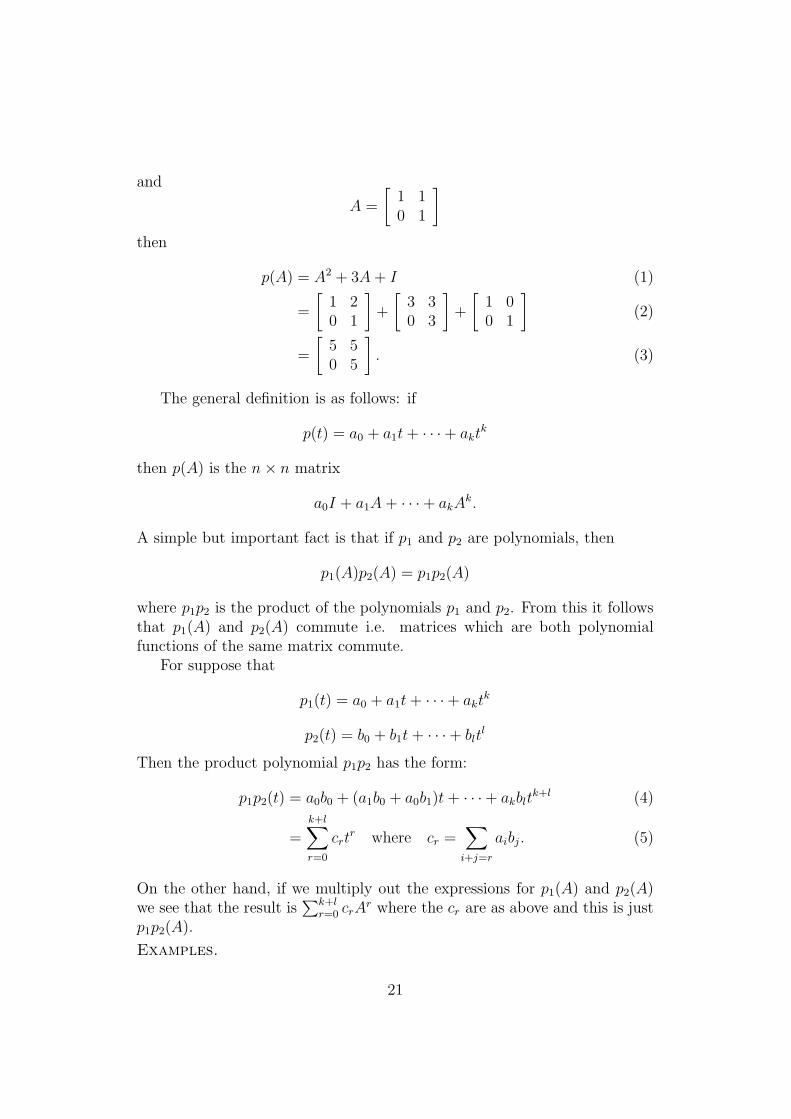
and

A =

[

1 10 1

]

then

p(A) = A2 + 3A+ I (1)

=

[

1 20 1

]

+

[

3 30 3

]

+

[

1 00 1

]

(2)

=

[

5 50 5

]

. (3)

The general definition is as follows: if

p(t) = a0 + a1t+ · · ·+ aktk

then p(A) is the n× n matrix

a0I + a1A + · · ·+ akAk.

A simple but important fact is that if p1 and p2 are polynomials, then

p1(A)p2(A) = p1p2(A)

where p1p2 is the product of the polynomials p1 and p2. From this it followsthat p1(A) and p2(A) commute i.e. matrices which are both polynomialfunctions of the same matrix commute.

For suppose that

p1(t) = a0 + a1t+ · · ·+ aktk

p2(t) = b0 + b1t + · · ·+ bltl

Then the product polynomial p1p2 has the form:

p1p2(t) = a0b0 + (a1b0 + a0b1)t + · · ·+ akbltk+l (4)

=

k+l∑

r=0

crtr where cr =

∑

i+j=r

aibj . (5)

On the other hand, if we multiply out the expressions for p1(A) and p2(A)we see that the result is

∑k+l

r=0 crAr where the cr are as above and this is just

p1p2(A).

Examples.

21

1) If A = diag (λ1, . . . , λn), then

p(A) = diag (p(λ1), . . . , p(λn)).

2) If p can be split into linear factors

(t− λ1) · · · (t− λk)

thenp(A) = (A− λ1I) · · · (A− λkI).

3) If A is the matrix Jn(λ) introduced above, then

p(A) =

p(λ) p′(λ) . . . p(n−1)(λ)(n−1)!

0 p(λ) . . . p(n−2)(λ(n−2)!

......

0 0 . . . p(λ)

.

Perhaps the easiest way to see this is to note first that it suffices to verifyit for the monomials tr (r = 0, 1, 2, . . . ) and this can be proved quite easilyusing induction on r. One interesting way to do it is as follows: Jn(λ) canbe expressed as the sum

λ 0 . . . 00 λ . . . 0...

...0 0 . . . λ

+

0 1 . . . 00 0 . . . 0...

...0 0 . . . 0

i.e. as λIn + Jn(0) where both matrices commute. This allows us to use thefollowing version of the binomial theorem to calculate the powers of Jn(λ).Let A and B be commuting n× n matrices. Then for r ∈ N,

(A+B)r =

r∑

k=0

(

r

k

)

AkBr−k.

This is proved by induction exactly as in the scalar case. We apply this tothe above representation of Jn(λ) and note that for r ≤ n, the r-th powerof Jn(0) is the matrix with zeros everywhere except for the diagonal whichbegins at the r-th element of the first row and which contains 1’s. If r ≥ n,then Jn(0)

r = 0.A final operation on matrices whose significance will become clear later is

that of transposition. If A = [aij] is an m× n matrix, then the transposed

22

matrix At is the n × m matrix [bij ] where bij = aji i.e. the rows of At arejust the columns of A. For example

1 1 0 0 00 1 2 0 00 0 1 3 00 0 0 1 40 0 0 0 1

t

=

1 0 0 0 01 1 0 0 00 2 1 0 00 0 3 1 00 0 0 4 1

.

The following simple properties can be easily checked:

• (A+B)t = At +Bt;

• (AB)t = BtAt.

• if A is invertible, then so is At and (At)−1 = (A−1)t (for (At)(A−1)t =(A−1 · A)t = I t = I);

• (At)t = A.

Examples. Calculate the inverse of the n× n matrix

0 1 1 . . . 11 0 1 . . . 1...

...1 1 1 . . . 0

.

This corresponds to the system

x2 + . . . + xn = y1x1 + x3 . . . + xn = y2

......

x1 + x2 . . . + xn−1 = yn.

Adding, we get the additional equation

x1 + · · ·+ xn =1

n− 1(y1 + · · ·+ yn)

and so

x1 =1

n− 1(y1 + · · ·+ yn)− y1 (6)

=1

n− 1(−(n− 2)y1 + y2 + . . . yn) (7)

23

etc. Hence the required inverse is the matrix

1

n− 1

−(n− 2) 1 . . . 11 −(n− 2) . . . 1...

...1 1 . . . −(n− 2)

.

Exercises :1) What are the matrices of the following systems

x+ y = 0 a1x1 + . . . + anxn = 0y + z = 0 a1x2 + . . . + anx1 = 0

z + u = 0...

u+ x = 0 a1xn + . . . + anxn−1 = 0?

2) Calculate AB and BA where

A =

cos θ − sin θ 0sin θ cos θ 00 0 1

B =

1 0 00 cosφ − sinφ0 sin φ cos φ

.

3) Give examples of matrices A, B, C, D, E, F , G, J and K so that

• A2 = −I;

• B2 = 0 but B 6= 0;

• CD = −DC but neither is zero;

• EF = 0 but each element of E resp. F is non-zero;

• G3 = 0 but G2 6= 0;

• J = J t, K = Kt but (JK)t 6= JK.

4) Let

C =

[

c11 c12c21 c22

]

be a matrix with c11 + c22 = 0. Show that there are 2× 2 matrices A and Bwith C = AB−BA. (Why have we insisted on the condition c11 + c22 = 0?)5) Determine all 2× 2 matrices

A =

[

a bc d

]

24

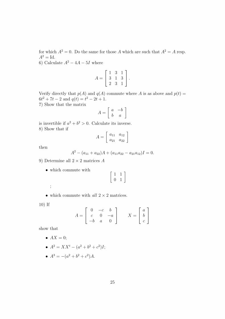
for which A2 = 0. Do the same for those A which are such that A2 = A resp.A2 = Id.6) Calculate A2 − 4A− 5I where

A =

1 3 13 1 32 3 1

.

Verify directly that p(A) and q(A) commute where A is as above and p(t) =6t2 + 7t− 2 and q(t) = t2 − 2t+ 1.7) Show that the matrix

A =

[

a −bb a

]

is invertible if a2 + b2 > 0. Calculate its inverse.8) Show that if

A =

[

a11 a12a21 a22

]

thenA2 − (a11 + a22)A+ (a11a22 − a21a12)I = 0.

9) Determine all 2× 2 matrices A

• which commute with[

1 10 1

]

;

• which commute with all 2× 2 matrices.

10) If

A =

0 −c bc 0 −a−b a 0

X =

abc

show that

• AX = 0;

• A2 = XX t − (a2 + b2 + c2)I;

• A3 = −(a2 + b2 + c2)A.

25

Calculate A921.11) Calculate p(C) where

p(t) = a0 + a1t + · · ·+ an−1tn−1

and C is the n× n matrix

0 1 0 . . . 00 0 1 . . . 0...

...1 0 0 . . . 0

.

12) If A and B are n×n matrices and we put [A,B] = AB−BA, show that

[A, [B,C]] + [B, [C,A]] + [C, [A,B]] = 0.

13) Show that if A is an n× n matrix with aij = 0 for i ≤ j, then An = 0.14) Show that if an m× n matrix A is such that AtA = 0, then A = 0.15) Let C denote the matrix of example 11) and let A be the typical n × nmatrix. Calculate CAC, CACt, CAC−1.

If Ap = Cp + C−p, show that

Ap = An−p (8)

ApAq = Ap+q + Ap−q (9)

Ap+1 = A1Ap −Ap−1. (10)

16) If A is a n× n matrix, we define As (s ∈ R) to be (sI − A)−1 wheneverthis inverse exists. Show that

(t− s)AtAs = As − At.

17) Sei T the n× n matrix

0 0 . . . 0 10 0 . . . 1 0... 00 1 . . . 0 01 0 . . . 0 0

.

If A is the general n × n matrix [aij ], calculate AT , TA, TAT , AtT , TAtT .

Describe those matrices B which commute with T .18) Show that the product of two triangular matrices is triangular. Showthat if the diagonal elements of a triangular matrix are all positive, then

26

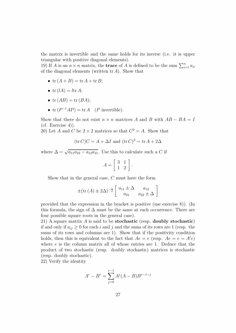
the matrix is invertible and the same holds for its inverse (i.e. it is uppertriangular with positive diagonal elements).19) If A is an n× n matrix, the trace of A is defined to be the sum

∑n

i=1 aiiof the diagonal elements (written trA). Show that

• tr (A+B) = trA+ trB;

• tr (lA) = ltrA;

• tr (AB) = tr (BA);

• tr (P−1AP ) = trA (P invertible).

Show that there do not exist n × n matrices A and B with AB − BA = I(cf. Exercise 4)).20) Let A and C be 2× 2 matrices so that C2 = A. Show that

(trC)C = A +∆I and (trC)2 = trA + 2∆

where ∆ =√a11a22 − a12a21. Use this to calculate such a C if

A =

[

3 11 2

]

.

Show that in the general case, C must have the form

±(tr (A)± 2∆)−12

[

a11 ±∆ a12a21 a22 ±∆

]

provided that the expression in the bracket is positive (use exercise 8)). (Inthis formula, the sign of ∆ must be the same at each occurrence. There arefour possible square roots in the general case).21) A square matrix A is said to be stochastic (resp. doubly stochastic)if and only if aij ≥ 0 for each i and j and the sums of its rows are 1 (resp. thesums of its rows and columns are 1). Show that if the positivity conditionholds, then this is equivalent to the fact that Ae = e (resp. Ae = e = Ate)where e is the column matrix all of whose entries are 1. Deduce that theproduct of two stochastic (resp. doubly stochastic) matrices is stochastic(resp. doubly stochastic).22) Verify the identity

Ar −Br =

r−1∑

j=0

Aj(A− B)Br−1−j

27

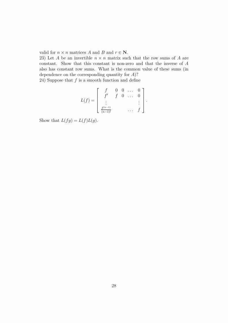
valid for n× n matrices A and B and r ∈ N.23) Let A be an invertible n × n matrix such that the row sums of A areconstant. Show that this constant is non-zero and that the inverse of Aalso has constant row sums. What is the common value of these sums (independence on the corresponding quantity for A)?24) Suppose that f is a smooth function and define

L(f) =

f 0 0 . . . 0f ′ f 0 . . . 0...

...f(n−1)

(n−1)!. . . f

.

Show that L(fg) = L(f)L(g).

28

1.3 Matrix multiplication, Gaußian eliminationand hermitian forms

We now turn to a more detailed study of the method used to solve thegeneral system AX = Y in the light of the arithmetical operations. Thisconsisted in the following procedure. At the i-th step, we examined the last(m − i + 1) equations and located that one which had the lowest indexednon-zero coefficient (in general there will be several of them). We exchangedone of these equations with the i-th one and arranged (by division) for itto have leading coefficient 1. By subtracting suitable multiples of the i-thequation from the later ones we ensured that their leading coefficients all layto the right of that of the i-th equation. The procedure stopped after thatstep r for which the last (m−r) equations were trivial (i.e. were such that allcoefficients were zero). The matrix of the new system then had the followingform

B1

B2...Br

0...0

where the i-th row Bi is

[

0 0 . . . 0 1 ai,ji+1 . . . ain]

for some strictly increasing sequence 1 ≤ j1 < j2 < · · · < jr ≤ n where thepivotal 1’s (which are in bold type) are in the columns j1, j2, . . . , jr. Amatrix with this structure is said to be in Hermitian form (or to be anechelon matrix).

Note that in carrying out the algorithm we apply at each step one of thefollowing three so-called elementary operations on the rows of A:I. Addition of λ times row i to row j for some scalar λ. In symbols:

A1...Ai

...Aj

...Am

7→

A1...Ai

...Aj + λAi

...Am

.

29

(This was used to eliminate unwanted coefficients).II. Exchanging row i with row j:

A1...Ai

...Aj

...Am

7→

A1...Aj

...Ai

...Am

.

(This was used to obtain a non-zero pivot by exchanging equations).III. Multiplying the i-th row by a non-zero scalar λ.

A1...Ai

...Am

7→

A1...

λAi

...Am

(in order to obtain 1 as the leading coefficient).We now make the simple observation that each of these operations can

be realised by left multiplication by a suitable m×m matrix:I. Left multiplication by the matrix P λ

ij where the latter is the matrix [akl]with akl = 1 if k = l, akl = λ if k = i and l = j and akl = 0 otherwise.II. Left multiplication by Uij where the latter is the matrix [akl] with akl = 1if k = l and k is neither i or j, akl = 1 if k = i, l = j or k = j, k = l andakl = 0 otherwise.III. Left multiplication byMλ

i where the latter is the matrix [akl] with akl = 1if k = l and both are distinct from i and akl = λ if k = l = i. Otherwiseakl = 0.

Note that the above matrices are those which one obtains from the unitmatrix Im by applying the appropriate row operations. Matrices of the aboveform are called elementary matrices. Each of them is invertible and wehave the relationships:

(P λij)

−1 = P−λij U−1

ij = Uij (Mλi )

−1 =M1λ

i .

Since each step in the reduction to Hermitian form is accomplished byleft multiplication by an invertible matrix, we have the following result:

Proposition 3 Let A be an m × n matrix. Then there exists an invertiblem×m matrix B so that A = BA has Hermitian form.

30

Proof. For suppose that the reduction employs k steps whereby the i-thstep involves left multiplication by the matrix Pi. Then we have

Pk . . . P2P1A = A

and so B = Pk . . . P1 is the required matrix. That B is invertible followsfrom the following simple result:

Proposition 4 Let P1, . . . ,, Pk be invertible m × m matrices. Then theirproduct

Pk . . . P1

is invertible and its inverse is P−11 . . . P−1

k .

Proof. We simply multiply the product on the left and on the right by theproposed inverse and cancel (notice the order of the factors in the inverse).

We remark that neither B or A are uniquely determined by A.We now examine the transformed equation AX = Z. Note that we

now have a new right hand side Z = BY i.e. Z is obtained from Y byapplying the same row operations. The equation is then solvable if and onlyif zr+1 = · · · = zm = 0 and we can then write down the solution explicitly asfollows

xjr+1, . . . , xn are arbitrary; (11)

xjr = zr − ar,jr+1xjr+1 − · · · − arnxn; (12)

xjr−1+1, . . . , xjr−1 are arbitrary; (13)

xjr−1 = zr−1 − ar−1,jr−1+1xjr−1 + 1− · · · − ar−1,nxn; (14)

... (15)

xj1 = z1 − a1,j1+1xj1+1 − · · · − a1nxn; (16)

x1, . . . , xj1−1 are arbitrary. (17)

(Note that the solutions then contain (n− r) free parameters—the xi whichcorrespond to those columns which do not contain a pivotal 1).

Since the general systemAX = Y

is equivalent toAX = Z where Z = BY

we see that it is solvable if and only if the transformed column matrix Zis such that zr+1 = · · · = zm = 0 and the solution can be written down asabove.

31

A useful consequence of this analysis is the following: The equation AX =Y has a solution for any right hand side Y if and only if no row of thehermitian form A vanishes. The equation AX = 0 has only the trivialsolution X = 0 if and only if each column of A has a pivotal 1. Then m ≥ nand the last n−m rows vanish.

Once again, the solution contains n− r free parameters. In particular, ifn > r the homogeneous equation AX = 0 (and hence AX = 0) has a nontrivial solution (i.e. a solution other than X = 0). Since this is automaticallythe case if m < n, we get the following result.

Proposition 5 Every homogeneous system AX = 0 of m equations in nunknowns has a non-trivial solution provided that m < n.

In some applications it is often useful to be able to calculate the matrixB which reduces A to Hermitian form. An economical way to do this isto keep track of the matrices inducing the row operations by extending Ato the m × (m + n) matrix [A Im]. If we apply to the whole matrix therow operations employed to bring A into Hermitian form, then the requiredmatrix B will be the right hand m×m block at the end of the process.

Examples. We calculate a Hermitian form for the matrix

2 3 −1 13 2 −2 25 0 −4 4

.

We get successively:

2 3 −1 13 2 −2 25 0 −4 4

1 32

−12

12

3 2 −2 25 0 −4 4

1 32

−12

12

0 −52

−12

12

0 −152

−32

32

1 32

−12

12

0 1 15

−15

0 5 1 −1

1 32

−12

12

0 1 15

−15

0 0 0 0

.

32

(In the second last step we multiplied the last row by2

3to simplify the

arithmetic).

Examples. For

A =

5 3 8 92 −1 2 31 0 1 03 4 5 6

we find an invertible 4 × 4 matrix B so that BA has Hermitian form. Weextend A as above and obtain successively the following matrices:

5 3 8 9 1 0 0 02 −1 2 3 0 1 0 01 0 1 0 0 0 1 03 4 5 6 0 0 0 1

1 0 1 0 0 0 1 05 3 8 9 1 0 0 02 −1 2 3 0 1 0 03 4 5 6 0 0 0 1

1 0 1 0 0 0 1 00 3 3 9 1 0 −5 00 −1 0 3 0 1 −2 00 4 2 6 0 0 −3 1

1 0 1 0 0 0 1 00 −1 0 3 0 1 −2 00 3 3 9 1 0 −5 00 4 2 6 0 0 −3 1

1 0 1 0 0 0 1 00 −1 0 3 0 1 −2 00 0 3 18 1 3 −11 00 0 2 18 0 4 −11 1

1 0 1 0 0 0 1 00 −1 0 3 0 1 −2 00 0 1 6 1

31 −11

30

0 0 1 9 0 2 −112

12

1 0 1 0 0 0 1 00 −1 0 3 0 1 −2 00 0 1 6 1

31 −11

30

0 0 0 3 −13

1 −116

12

.

33

Hence

BA =

1 0 1 00 1 0 −30 0 1 60 0 0 1

where

B =

0 0 1 00 −1 2 013

1 113

0−1

913

−1118

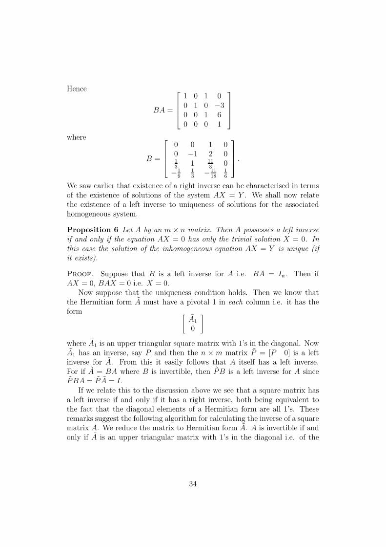
16

.

We saw earlier that existence of a right inverse can be characterised in termsof the existence of solutions of the system AX = Y . We shall now relatethe existence of a left inverse to uniqueness of solutions for the associatedhomogeneous system.

Proposition 6 Let A by an m× n matrix. Then A possesses a left inverseif and only if the equation AX = 0 has only the trivial solution X = 0. Inthis case the solution of the inhomogeneous equation AX = Y is unique (ifit exists).

Proof. Suppose that B is a left inverse for A i.e. BA = In. Then ifAX = 0, BAX = 0 i.e. X = 0.

Now suppose that the uniqueness condition holds. Then we know thatthe Hermitian form A must have a pivotal 1 in each column i.e. it has theform

[

A1

0

]

where A1 is an upper triangular square matrix with 1’s in the diagonal. NowA1 has an inverse, say P and then the n × m matrix P = [P 0] is a leftinverse for A. From this it easily follows that A itself has a left inverse.For if A = BA where B is invertible, then PB is a left inverse for A sincePBA = P A = I.

If we relate this to the discussion above we see that a square matrix hasa left inverse if and only if it has a right inverse, both being equivalent tothe fact that the diagonal elements of a Hermitian form are all 1’s. Theseremarks suggest the following algorithm for calculating the inverse of a squarematrix A. We reduce the matrix to Hermitian form A. A is invertible if andonly if A is an upper triangular matrix with 1’s in the diagonal i.e. of the

34

form

1 b12 b13 . . . b1n0 1 b23 . . . b2n...

...0 0 0 . . . 1

.

Now we can reduce this matrix to the unit matrix by further row operations.Thus by subtracting b12 times the first row from the second one we eliminatethe element above the diagonal one. Carrying on in the obvious way, we caneliminate all the non-diagonal elements. If we once more keep track of therow operations with the aid of an added right hand block, we end up with amatrix B which is invertible and such that BA = I. B is then the inverse ofA.

Examples. We calculate the inverse of

2 1 14 1 0−2 2 1

.

We expand the matrix as suggested above:

2 1 1 1 0 04 1 0 0 1 0−2 2 1 0 0 1

.

Successive row operations lead to the following sequence of matrices:

2 1 1 1 0 00 −1 −2 −2 1 00 3 2 1 0 1

2 1 1 1 0 00 −1 −2 −2 1 00 0 −4 −5 3 1

2 0 −1 −1 1 00 −1 −2 −2 1 00 0 −4 −5 3 1

2 0 0 14

14

14

0 −1 0 12

−12

−12

0 0 −4 −5 3 1

35

1 0 01

8

1

8−1

8

0 1 0 −1

2

1

2

1

2

0 0 15

4−3

4−1

4

.

Hence the inverse of A is

1

8

1

8−1

8

−1

2

1

2

1

25

4−3

4−1

4

.

We conclude this section with some general remarks on the method ofGaußian elimination.I. In carrying out the elimination, it was necessary to arrange for the pivotelements to be non-zero. In numerical calculations, it is advantageous toarrange for it to be as large as possible. This can be achieved by using aso-called column pivotal search which means that while choosing the pivotalelement in the k-th row, we replace the latter by that row which follows itand which has the largest initial element (in absolute value).

An even more efficient method is that of a complete pivot search. Hereone arranges for the largest element in the bottom right hand block to takeon the position of the pivotal element at the top left hand corner (of course,this involves exchanging rows and columns).II. If the pivot element at each stage is non-zero, in which case no row ex-changes are necessary, then the matrix B which transforms A into hermitianform A is lower triangular. In particular, if A is n × n (and so invertible),then A can be factorised as A = LU where L is lower triangular (it is theinverse of B) and U is upper triangular (it is the Hermitian form of A). Thisis call a lower-upper factorisation of A. Notice that then the equationAX = Y is equivalent to the two auxiliary ones

LZ = Y

andUX = Z

which can be solved immediately since their matrices are triangular.Not every invertible matrix has a lower-upper factorisation—for example

the 2× 2 matrix[

0 11 0

]

36

has no such factorisation. However, as we know from the method of elimi-nation, if A is invertible, then we can arrange, by permuting the rows of A,for the pivotal elements to be non-vanishing. This is achieved by left mul-tiplication by a so-called permutation matrix P i.e. the matrix which isobtained by permuting the rows of In in the same manner. Hence a generalinvertible matrix A has a factorisation A = QLU where Q is a permutationmatrix (the inverse of the P above), L is lower triangular and U is uppertriangular.

Exercises: 1) Calculate a Hermitian form for the matrices:

2 3 −1 13 2 −2 25 0 −4 4

1 −2 3 −12 −1 2 23 1 2 3

.

2) Find an invertible matrix B so that BA is in Hermitian form where

A =

5 3 8 92 −1 2 31 0 1 03 4 5 6

.

3) Calculate the general solutions of the systems:

2x + 3y − z + w = 33x + 2y − 2z + 2w = 05x − 4z + 4w = 6

resp.[

x + 2y + 3z + 4w = 102x + 3y + z + w = 3.

]

4) Calculate the inverses of the matrices

1 0 22 2 2−1 3 4

1 0 0 0 0a 1 0 0 00 b 1 0 00 0 c 1 00 0 0 d 1

.

5) Show that every invertible n × n matrix is a product of matrices of the

37

following forms:

0 0 0 . . . 11 0 0 . . . 00 1 0 . . . 0...

...0 0 0 . . . 00 0 . . . 1 0

0 1 0 . . . 01 0 0 . . . 00 0 1 . . . 0...

...0 0 0 . . . 1

1 k 0 . . . 00 1 0 . . . 0...

...0 0 0 . . . 1

λ 0 0 . . . 00 1 0 . . . 0... :

...0 0 0 . . . 1

(where k ∈ R and λ ∈ R \ {0}).6) We have seen that if the pivot elements of the matrix do not vanish,then we have a representation A = LU of A as a product of a lower and anupper triangular matrix. It is convenient to vary this representation a littlein order to obtain a unique one. Show that if A is as above, then it has aunique representation as a product LDU where D is a diagonal matrix andL and U are as above, except that we require them to have 1’s in their maindiagonals.

38

1.4 The rank of a matrix

In preparation for later developments we review what we have achieved sofar in a more abstract language. We are concerned with the mapping

fA : X 7→ AX

from the set of n× 1 matrices into the set of m× 1 matrices. We note someof its elementary properties:

• it is additive i.e.

fA(X1 +X2) = fA(X1) + f(X2).

Hence we can obtain a solution of the equation AX = Y1+Y2 by takingthe sum of solutions of AX = Y1 resp. AX = Y2;

• the mapping is homogeneous i.e. fA(λx) = λfA(X).

We can combine these two properties into the following single one:

fA(λ1X1 + λ2X2) = λ1fA(X1) + λ2fA(X2).

Mappings with this property are called linear. It then follows that for scalarsλ1, . . . , λr and n× 1 matrices X1, . . . , Xr we have:

fA(λ1X1 + · · ·+ λrXr) = λ1fA(X1) + · · ·+ λrfA(Xr).

In the light of these facts it is convenient to introduce the following notation:an n× 1 matrix X is called a (column) vector. A vector of the form λ1X1 +· · · + λrXr is called a linear combination of the vectors Xi. The Xi arelinearly independent if there are no scalars λ1, . . . , λr (not all zero) so thatλ1X1 + . . . λrXr = 0. Otherwise they are linearly dependent.

These terms are motivated by a geometrical interpretation which will betreated in detail in the following chapters. We note now that1) the equation AX = Y has a solution if and only if Y is a linear combinationof the columns of A. For the fact that the equation has a solution x1, . . . , xncan be expressed in the equation

x1A1 + · · ·+ xnAn = Y

where the Ai are the columns of A.2) any linear combination of solutions of the homogeneous equation AX = 0is itself a solution. This equation has the unique solution X = 0 if and onlyif the columns of A are linearly independent.

39

3) if X is a solution of the equation AX = Y and X0 is any solution of thecorresponding homogeneous equation AX = 0, then X0+X is also a solutionof AX = Y . Conversely, every solution of the latter is of the form X0 +Xwhere X0 is a solution of AX = 0. Hence in order to find all solutions ofAX = Y it suffices to find one particular solution and to find all solutionsof the homogeneous equation.4) the equation AX = Y has at most one solution if and only if the homoge-neous equation AX = 0 has only the trivial solution X = 0 i.e. if and onlyif the columns of A are linearly independent.

The reader will notice that all these facts follow from the linearity of fA.In the light of these remarks it is clear that the following concept will

play a important role in the theory of systems of equations:

Definition: Let A be an m × n matrix. The column rank of A is themaximal number of linearly independent columns in A (we shall see shortlythat this is just the number r of non-vanishing rows in the Hermitian formof A).

In principle one could calculate this rank as follows: we investigate suc-cessively the columns A1, A2, . . . of A and discard those ones which are linearcombinations of the preceding ones. Eventually we obtain a matrix A whosecolumns are linear independent. Then the column rank of A (and also of A)is r, the number of columns of A.

We can also define the concept of row rank in an analogous manner. Ofcourse it is just the column rank of At. We shall now show that the row rankand the column rank coincide so that we can talk of the rank of A, writtenr(A). In order to do this we require the following Lemma:

Lemma 1 Let A = [A1 . . . An] be an m × n matrix and suppose that A =[A1 . . . Aj−1Aj+1 . . . An] is obtained by omitting the column Aj which is alinear combination of A1, . . . , Aj−1. Then the row ranks of A and A coincide.

Proof. The assumption on A means that it can be written in the form

A =[

A1 . . . Aj−1 λ1A1 + · · ·+ λj−1Aj−1 Aj+1 . . . An

]

for suitable scalars λ1, . . . , λj−1. Now suppose that some linear combina-tion of the rows of A is zero. Then since the elements {aij}mi=1 of the extracolumn in A are obtained as linear combinations of the components of thecorresponding rows, we see that the same linear combination of the rows ofA vanish and this means that a set of rows of A is linearly independent ifand only if the corresponding rows of A are.

40

Proposition 7 If A is an m× n matrix, then the row rank and the columnrank of A coincide.

Proof. We apply the method described above to reject suitable columns ofA and obtain an m× s matrix B with linearly independent columns, wheres is the columns rank of A. We now proceed to apply the same method tothe rows of B to obtain an r × s matrix with independent rows where r isthe row rank of B and so, by the Lemma, also of A. now we know that thereexist at most s linearly independent s-vectors and so r ≤ s (this follows fromthe result on the existence of non-trivial soutions of homogeneuos systems).Similarly s ≤ r and the proof is done.

Remark: Usually the most effective method of calculating the rank of amatrix A is as follows: one calculates a Hermitian form A for A. Then therank of A is the number of non-vanishing rows of A. For each elementary rowoperation clearly leaves the row rank of A unchanged and so the row ranksof A and A coincide. But the non-zero rows of a matrix in Hermitian formare obviously linearly independent and so the rank of A is just the numberof its non-vanishing rows.

Examples. We illustrate this by calculating the rank of

3 −1 4 62 0 −2 60 3 1 40 1 1 −32 2 2 0

.

We reduce to hermitian form with row operations to obtain successively thematrices:

3 −1 4 62 0 −2 60 3 1 40 1 1 −32 2 2 0

resp.

1 0 −1 30 1 1 −30 3 1 42 2 2 03 −1 4 6

41

resp.

1 0 −1 30 1 1 −30 3 1 40 2 4 −60 −1 7 −3

resp.

1 0 −1 30 1 1 −30 0 −2 130 0 2 00 0 8 −6

resp.

1 0 −1 30 1 1 −30 0 0 130 0 2 00 0 0 −6

resp.

1 0 −1 30 1 1 −30 0 1 00 0 0 10 0 0 0

and so the rank is 4.

Examples. We calculate the rank of the matrix

A =

3 −1 4 62 0 −2 60 3 1 40 1 1 −32 2 2 0

.

Solution: We reduce to Hermitian form as follows:

3 −1 4 62 0 −2 60 3 1 40 1 1 −32 2 2 0

42

1 0 −1 30 1 1 −30 3 1 42 2 2 03 −1 4 6

1 0 −1 30 1 1 −30 3 1 40 2 4 −60 −1 7 3

1 0 −1 30 1 1 −30 0 −2 130 0 2 00 0 8 −6

1 0 −1 30 1 1 −30 0 0 130 0 2 00 0 0 −6

1 0 −1 30 1 1 −30 0 1 00 0 0 10 0 0 0

.

Hence r(A) = 4.With this characterisation of rank, the relationship between the Hermi-

tian form and the solvability resp. uniqueness of solutions of the equationAX = Y can be restated as follows:

Proposition 8 Let A be an m× n matrix. Then

• the equation AX = Y is always solvable if and only if r(A) = m andthis is equivalent to the fact that A has a right inverse;

• the equation AX = 0 has only the trivial solution if and only if r(A) = nand this is equivalent to the fact that A has a left inverse.

In particular, if A is square, then it has a left inverse if and only if it has aright inverse and in either case it is invertible (as we have already above).

43

Exercises: 1) Calculate the ranks of the following matrices:

1 0 22 0 46 0 01 0 2

3 −1 4 62 0 −2 60 1 1 −32 2 1 0

.

2) If A is an m×n matrix of rank 1, then there exist (ξi) ∈ Rm and (ηi) ∈ Rn

so that A = [ξiηj].3) Show that if A and B are m× n matrices so that

r(A) = r(B) = r(A+B) = 1,

then there is an 1× n matrix X and scalars λ1, . . . , λm, µ1, . . . , µm so that

A =

λ1X...

λmX

B =

µ1X...

µmX

or the corresponding result holds for At and Bt.4) Show that the equation AX = Y is solvable if and only if r(A) = r([A, Y ]).5) Show that r(A) ≤ 2 where A is the n × n matrix [sin(ai + bj)]

ni,j=1 ((ai)

and (bj) are arbitrary sequences of real numbers).

44

1.5 Matrix equivalence

We have seen that we can reduce a matrix to Hermitian form by multiplyingon the left by an invertible matrix. We now consider the simplifications whichare possible if we are allowed also to multiply on the right by such matrices—equivalently, by multiplying on the right by the elementary matrices P λ

ij, Uij

and Mλk . Now it is easy to check that these operations produce the following

effects:

• right multiplication by P λji adds λ times the i-th column to the j-th

column; right multiplication by Uij exchanges column i and column j;right multiplication by Mλ

i multiplies column i by λ.

Let us consider what we can achieve by means of these operations. Startingwith a matrix in Hermitian form we can, by exchanging columns, bring allof the leading 1’s into the main diagonal. Now, by successively subtractingsuitable multiples of the first column from the others we can arrange for allof the entries in the first row (with the exception of the initial 1 of course)to vanish. Similarly, by working with column 2 we can annihilate all of theentries of the second row (except for the 1 in the diagonal). Proceeding inthe obvious way we obtain a matrix of the form

1 0 . . . 0 . . . 00 1 . . . 0 . . . 0...

...0 . . . 1 . . . 00 . . . 0...

...0 . . . 0

where the final 1 is in the r-th row. We denote this matrix symbolically by[

Ir 00 0

]

.

We have thus proved the following:

Proposition 9 If A is an m × n matrix, then there are invertible matricesP (m×m) and Q ( n× n) so that

PAQ =

[

Ir 00 0

]

where r is the rank of A.

45

We introduce the following notation: We say that two m×n matrices A andB are equivalent when matrices P and Q as in the Proposition exist so thatPAQ = B. Then this result states that A is equivalent to a matrix of theform

[

Ir 00 0

]

whereby r = r(A).It follows easily that two matrices are equivalent if and only if they have

the same rank.In order to calculate such P and Q for a specific matrix we proceed in a

manner similar to that used to calculate inverses except that we keep trackof the column operations by adding a second unit matrix, this time belowthe original one. We illustrate this with the example

A =

2 1 1 1−2 1 2 0−2 3 5 1

.

The expanded matrix is

2 1 1 1 1 0 0−2 1 2 0 0 1 0−2 3 5 1 0 0 11 0 0 00 1 0 00 0 1 00 0 0 1

.

We then compute as follows:

2 1 1 1 1 0 0−2 1 2 0 0 1 0−2 3 5 1 0 0 11 0 0 00 1 0 00 0 1 00 0 0 1

2 1 1 1 1 0 00 2 3 1 1 1 00 4 6 2 1 0 11 0 0 00 1 0 00 0 1 00 0 0 1

46

2 1 1 1 1 0 00 2 3 1 1 1 00 0 0 0 −1 −2 11 0 0 00 1 0 00 0 1 00 0 0 1

2 0 0 0 1 0 00 2 3 1 1 1 00 0 0 0 −1 −2 11 −1

2−1

2−1

2

0 1 0 00 0 1 00 0 0 1

2 0 0 0 1 0 00 2 0 0 1 1 00 0 0 0 −1 −2 11 −1

214

−14

0 1 −32

−12

0 0 1 00 0 0 1

.

Hence if

Q =1

2

1 −12

14

−14

0 1 −32

−12

0 0 1 00 0 0 1

and

P =

1 0 01 1 0−1 −2 1

then we have

PAQ =

1 0 0 00 1 0 00 0 0 0

.

As an application of this representation we show that left or right multipli-cation by a matrix cannot increase the rank of A.

Proposition 10 If A and B are matrices so that the product AB is defined,then the rank r(AB) of the latter is less than or equal to both r(A) and r(B)(i.e. r(AB) ≤ min(r(A), r(B))).

47

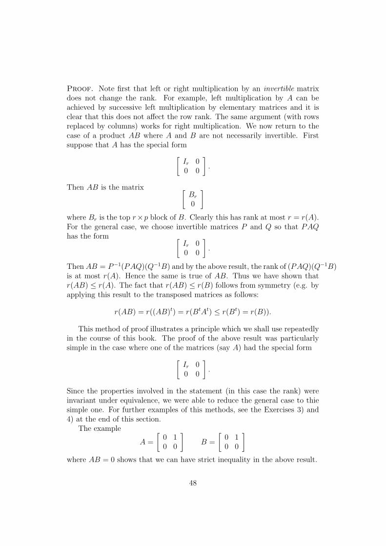
Proof. Note first that left or right multiplication by an invertible matrixdoes not change the rank. For example, left multiplication by A can beachieved by successive left multiplication by elementary matrices and it isclear that this does not affect the row rank. The same argument (with rowsreplaced by columns) works for right multiplication. We now return to thecase of a product AB where A and B are not necessarily invertible. Firstsuppose that A has the special form

[

Ir 00 0

]

.

Then AB is the matrix[

Br

0

]

where Br is the top r×p block of B. Clearly this has rank at most r = r(A).For the general case, we choose invertible matrices P and Q so that PAQhas the form

[

Ir 00 0

]

.

Then AB = P−1(PAQ)(Q−1B) and by the above result, the rank of (PAQ)(Q−1B)is at most r(A). Hence the same is true of AB. Thus we have shown thatr(AB) ≤ r(A). The fact that r(AB) ≤ r(B) follows from symmetry (e.g. byapplying this result to the transposed matrices as follows:

r(AB) = r((AB)t) = r(BtAt) ≤ r(Bt) = r(B)).

This method of proof illustrates a principle which we shall use repeatedlyin the course of this book. The proof of the above result was particularlysimple in the case where one of the matrices (say A) had the special form

[

Ir 00 0

]

.

Since the properties involved in the statement (in this case the rank) wereinvariant under equivalence, we were able to reduce the general case to thiesimple one. For further examples of this methods, see the Exercises 3) and4) at the end of this section.

The example

A =

[

0 10 0

]

B =

[

0 10 0

]

where AB = 0 shows that we can have strict inequality in the above result.

48

Exercises: 1) Find invertible matrices P and Q so that PAQ has the form

[

Ir 00 0

]

where

A =

3 1 10 0 06 2 23 1 1

resp.

A =

1 1 1 11 2 3 44 3 2 1

.

2) Show that if A is an m× n matrix with rank r, then A can be expressedin the form BC where B is an m× r matrix and C is an r× n matrix (bothnecessarily of rank r).3) Show that if A is an m× n matrix with r(A) = r, then A has a represen-tation

A = A1 + · · ·+ Ar

where each Ai has rank 1. (In this and the previous example, prove it firstlyfor the case of a matrix of the form

[

Ir 00 0

]

and then use the principle mentioned in the text.)4) Show that if A is an m× n matrix and B is n× p, then

r(AB) ≥ r(A) + r(B)− n.

Deduce that if r(A) = n, then r(AB) = r(B).5) Prove the inequality r(AB) + r(BC) ≤ r(B) + r(ABC) where A, B andC are m × n resp. n × p resp. p × q matrices (note in particular the caseB = I).

49

1.6 Block matrices

We now discuss a topic which is useful theoretically and can be helpful insimplifying calculations in specific examples. This consists of partitioning amatrix into smaller units or blocks. For example the 4× 4 matrix

A =

1 2 3 42 4 6 84 3 2 18 6 4 2

can be split into 4 2× 2 blocks as follows:

A =

1 2 3 42 4 6 8

4 3 2 18 6 4 2

which we write as

A =

[

A11 A12

A21 A22

]

where

A11 =

[

1 22 4

]

etc.The general scheme is as follows: let A be an m× n matrix and suppose

that0 = m0 ≤ m1 ≤ · · · ≤ mr = m

and0 = n0 ≤ n1 ≤ · · · ≤ ns = n.

We define (mi−mi−1)× (nj −nj−1) matrices Aij for 1 ≤ i ≤ r and 1 ≤ j ≤ sas follows:

Aij =

ami−1+1,nj−1+1 . . . ami−1+1,nj

......

ami,nj−1+1 . . . ami,nj

.

Then we write

A =

A11 . . . A1s...

...Ar1 . . . Ars

50

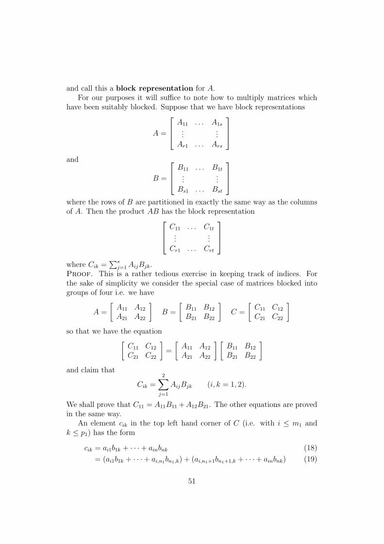
and call this a block representation for A.For our purposes it will suffice to note how to multiply matrices which

have been suitably blocked. Suppose that we have block representations

A =

A11 . . . A1s...

...Ar1 . . . Ars

and

B =

B11 . . . B1t...

...Bs1 . . . Bst

where the rows of B are partitioned in exactly the same way as the columnsof A. Then the product AB has the block representation

C11 . . . C1t...

...Cr1 . . . Crt

where Cik =∑s

j=1AijBjk.Proof. This is a rather tedious exercise in keeping track of indices. Forthe sake of simplicity we consider the special case of matrices blocked intogroups of four i.e. we have

A =

[

A11 A12

A21 A22

]

B =

[

B11 B12

B21 B22

]

C =

[

C11 C12

C21 C22

]

so that we have the equation[

C11 C12

C21 C22

]

=

[

A11 A12

A21 A22

] [

B11 B12

B21 B22

]

and claim that

Cik =

2∑

j=1

AijBjk (i, k = 1, 2).

We shall prove that C11 = A11B11 +A12B21. The other equations are provedin the same way.

An element cik in the top left hand corner of C (i.e. with i ≤ m1 andk ≤ p1) has the form

cik = ai1b1k + · · ·+ ainbnk (18)

= (ai1b1k + · · ·+ ai,n1bn1,k) + (ai,n1+1bn1+1,k + · · ·+ ainbnk) (19)

51

and the first bracket is the (i, k)-th element of A11B11 while the second is thecorresponding element of A12B21.

As a simple but useful application we have the following result:

Proposition 11 Let A be an n× n matrix with block representation[

B C0 D

]

where B is a square matrix. Then A is invertible if and only if B and D areand its inverse is the matrix

[

B−1 −B−1CD−1

0 D−1

]

.

Proof. Consider the matrix[

E FG H

]

as a candidate for the inverse. Multiplying out we get[

B C0 D

] [

E FG H

]

=

[

BE + CG BF + CHDG DH

]

.

If the right hand side is to be the unit matrix, we see immediately that wemust have DH = I i.e. D is invertible and H = D−1. Since DG = 0 and Dis invertible we see that G = 0. The equation now simplifies to

[

B C0 D

] [

E F0 D−1

]

=

[

BE BF + CD−1

0 I

]

.

Now we see that BE = I i.e. that B is invertible and E = B−1. Fromthe condition that BF + CD−1 = 0 it follows that F = −B−1CD−1. Thuswe have shown that if A is invertible then so are B and D and the inversehas the above form. On the other hand, if B and D are invertible, a simplecalculation shows that this matrix is, in fact, an inverse for A.

As an application, we calculate the inverse of the matrix:

cosα − sinα cos β − sin βsinα cosα sin β cos β0 0 cos γ − sin γ0 0 sin γ cos γ

.

Since the inverse of[

cosα − sinαsinα cosα

]

52

is[

cosα sinα− sinα cosα

]

it follows from the above formula and the result above on the product ofmatrices of this special form that the inverse is

cosα sinα − cos(α− β + γ) − sin(α− β + γ)− sinα cosα sin(α− β + γ) − cos(α− β + γ)

0 0 cos γ sin γ0 0 − sin γ cos γ

.

Exercises: 1) Show that if

A =

1 0 0 00 1 0 0a b −1 0c d 0 −1

then A2 = I.2) Calculate the product

1 1 0 0 0 02 1 0 0 0 00 0 3 1 2 00 0 1 2 1 00 0 0 1 1 10 0 0 0 0 1

1 2 3 4 5 62 3 4 5 6 73 4 5 6 7 84 5 6 7 8 95 6 7 8 9 106 7 8 9 10 11

.

3) Let C have block representation[

A −BB A

]

where A and B are commuting n× n matrices. Calculate C2 and

C

[

A B−B A

]

. Show that C is invertible if and only if A2 +B2 is invertible and calculateits inverse.4) Let the n× n matrix P have the block representation

[

A B0 D

]

53

where A (and hence D) is a square matrix. Show that if A is invertible, thenr(P ) = r(A) + r(D). Is the same true for general A (i.e. in the case whereA is not necessarily invertible)?5) Let A be an n× n matrix with block representation

[

A1 A2

alpha3 a

]

where A1 is an (n − 1) × (n − 1) matrix. Show that if A1 is invertible anda 6= A3A

−11 A2, then A is invertible and its inverse is

[

A1 A2

A3 a

]

where a = (a − A3A−11 A2)

−1, A3 = −aA3A−11 , A2 = −aA−1

1 A2 and A1 =A−1

1 (I − A2A3). (This exercise provides an algorithm which reduces thecalculation of the inverse of an n× n matrix to that of an (n− 1)× (n− 1)matrix).6) Calculate the inverse of a matrix of the form

A B C0 D E0 0 F

where A, D and F are non-singular square matrices.

54

1.7 Generalised inverses

We now present a typical application of block representations. We shall usethem, together with the reduction of an arbitrary matrix to the form

[

Ir 00 0

]

to construct so-called generalised inverses.Recall that if A is an n × n matrix, the inverse A−1 (if it exists) can be

used to solve the equation AX = Y—the unique solution being X = A−1Y .More generally, if the m × n matrix A has a right inverse B, then X = BYis a solution. On the other hand, if A has a left inverse C, the equationAX = Y need not have a solution but if it does have one for a particularvalue of Y , then this solution is unique.

The generalised inverse acts as a substitute for the above inverses andallows one to determine whether a given equation AX = Y has a solutionand, if so, provides such a solution (in fact, all solutions). More precisely, itis an n×m matrix S with the property that if AX = Y has a solution, thenthis solution is given by the vector X = SY . In addition, AX = Y has asolution if and only if ASY = Y .

We shall use the principle mentioned in the above section, namely webegin with the transparent case where A has the form

[

Ir 00 0

]

.

(The general case will follow readily). This corresponds to the system:

x1 . . . = y1x2 . . . = y2

......

xr . . . = yr

the remaining equations having the form 0 = yk (k = r + 1, . . . , m).Of course, this system has a solution if and only if yr+1 = · · · = ym = 0

and then a solution is X = SY where S is the n×m matrix[

Ir 00 0

]

.

Note that this matrix satisfies the two conditions:1) SAS = S;

55

2) ASA = A.We now turn to the case of a general m× n matrix A. An n×m matrix

S with the above two properties is called a generalised inverse for A. Thenext result shows that every matrix has a generalised inverse.

Proposition 12 Let A be an m× n matrix. Then there exists a generalisedinverse S for A.

Proof. We choose invertible matrices P and Q so that A = PAQ has theform

[

Ir 00 0

]

and let S be a generalised inverse for A. Then one can check that S = QSPis a generalised inverse for A. For

SAS = QSP (P−1AQ−1)QSP = QSASP = QSP = S

and

ASA = (P−1AQ−1)QSP (P−1AQ−1) = A.

The relevance of generalised inverses for the solution of systems of equa-tions which we discussed above is expressed formally in the next result:

Proposition 13 Let A be an m×n matrix with generalised inverse S. Thenthe equation AX = Y has a solution if and only if ASY = Y and then asolution is given by the formula X = SY . In fact, the general solution hasthe form

X = SY + (I − SA)Z

where Z is an arbitrary n× 1 matrix.

Proof. Clearly, if AX = Y , then ASY = ASAX = AX = Y and sothe above condition is fulfilled. On the other hand, if it is fulfilled i.e. ifASY = Y , then of course X = SY is a solution. To prove the second part,we need only show that the general solution of the homogeneous equationAX = 0 has the form (I − SA)Z. But if AX = 0, then SAX = 0 and soX = X − SAX = (I − SA)X and X has the required form. Of course avector of type (I − SA)Z is a solution of the homogeneous equation since

A(I − SA)Z = (A− ASA)Z = 0 · Z = 0.

56

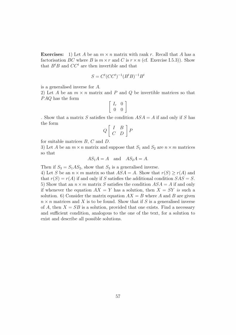
Exercises: 1) Let A be an m× n matrix with rank r. Recall that A has afactorisation BC where B is m× r and C is r×n (cf. Exercise I.5.3)). Showthat BtB and CCt are then invertible and that

S = Ct(CCt)−1(BtB)−1Bt

is a generalised inverse for A.2) Let A be an m × n matrix and P and Q be invertible matrices so thatPAQ has the form

[

Ir 00 0

]

. Show that a matrix S satisfies the condition ASA = A if and only if S hasthe form

Q

[

I BC D

]

P

for suitable matrices B, C and D.3) Let A be an m×n matrix and suppose that S1 and S2 are n×m matricesso that

AS1A = A and AS2A = A.

Then if S3 = S1AS2, show that S3 is a generalised inverse.4) Let S be an n×m matrix so that ASA = A. Show that r(S) ≥ r(A) andthat r(S) = r(A) if and only if S satisfies the additional condition SAS = S.5) Show that an n×m matrix S satisfies the condition ASA = A if and onlyif whenever the equation AX = Y has a solution, then X = SY is such asolution. 6) Consider the matrix equation AX = B where A and B are givenn× n matrices and X is to be found. Show that if S is a generalised inverseof A, then X = SB is a solution, provided that one exists. Find a necessaryand sufficient condition, analogous to the one of the text, for a solution toexist and describe all possible solutions.

57

1.8 Circulants, Vandermonde matrices

In this final section of Chapter I we introduce two special types of matriceswhich are of some importance.

Circulant matrices: These are matrices of the form

a1 a2 . . . anan a1 . . . an−1...

...a2 a3 . . . a1

.

Such a matrix is determined by its first row and so it is convenient to denoteit simply as

circ (a1, . . . , an).

For example, the identity matrix is circ (1, 0, . . . , 0). The next simplest cir-culant is circ (0, 1, . . . , 0). This is the matrix C which occurs in ExerciseI.2.11). It plays a central role in the theory of circulants since the fact thata matrix A be a circulant can be characterised by the fact that A satisfiesthe equation AC = CA (i.e. that A commutes with C). This can easilyseen by comparing the expressions for AC and CA calculated in the exercisementioned above. It follows easily from this characterisation that sums andproducts of circulants are themselves circulants.

The Vandermonde matrices: These are matrices of the form

V = V (t1, . . . , tn) =

1 1 . . . 1t1 t2 . . . tnt21 t22 . . . t2n...

...tn−11 tn−1

2 . . . tn−1n

.

They arise in the treatment of so-called interpolation problems. Supposethat we are given a sequence t1, . . . , tn of distinct points on the line. Forvalues y1, . . . , yn we seek a polynomial p of degree n−1 so that p(ti) = yi foreach i. If p has the form

p(t) = a0 + a1t + · · ·+ an−1tn−1

then we get the system

a0 + a1ti + · · ·+ an−1tn−1i = yi

58

(i = 1, . . . , n) of equations in the a’s. The matrix of this system is just V t,the transpose of V .

It is well-known that such interpolation problems always have a solution.This fact, which will be proved in VI.2, implies that the matrix V is invertible(under the assumption, of course, that the ti are distinct).

Another situation where the Vandermonde matrix arises naturally is thatof quadrature formulae. Let w be a positive, continuous function on theinterval [−1, 1] (a so-called weight function) and consider the problem ofcalculating numerically the weighted integral

∫ 1

−1

x(t)w(t) dt

of a continuous function x. A standard method of doing this is by discretisa-tion i.e. by supposing that we are given points t1, . . . , tn in the interval andpositive numbers w1, . . . , wn. We consider an approximation of the form

In(x) =

n∑

j=1

wjx(tj)

for the integral. A suitable criterium for determining whether this provides agood approximation is to demand that it be correct for polynomials of degreeat most n− 1. This leads to the equations

n∑

j=1

wjtkj = yk

for the w’s where yk =∫ 1

−1w(t)tk dt. Once again, the matrix of this equation

is V t. Since V is invertible, these equations can be solved and provide suitablevalues for the weights w1, . . . , wn.

Exercises: 1) Show that each circulant matrix is a polynomial in the spe-cial circulant C = circ(0, 1, . . . , 0).2) Calculate the square of the Vandermonde matrix V (t1, . . . , tn). 3) Calcu-late the inverse of the special Vandermonde matrix

V (0,1

n,2

n, . . . , 1)

(this is an (n+ 1)× (n+ 1) matrix).4) Describe the form of those circulant matrices A which satisfy one of thefollowing conditions:

59

a) At = A;b) At = −A;c) A is diagonal.

5) Which n × n matrices A satisfy the equation A = CAC where C is thecirculant matrix circ(0, 1, 0, . . . , 0)?6) Which n × n matrices A satisfy the equation AD = DA where D is thematrix

0 1 0 . . . 00 0 1 . . . 0...

...0 0 0 . . . 1−1 0 0 . . . 0

?

7) Calculate the inverses of the Vandermonde matrices

[

1 1s t

]

1 1 1s t us2 t2 u2

1 1 1 1s t u vs2 t2 u2 v2

s3 t3 u3 v3

.

Can you detect any pattern which would suggest a formula for the inverse ofthe general Vandermonde matrix?

60

2 ANALYTIC GEOMETRY IN 2 and 3 DI-

MENSIONS

2.1 Basic geometry in the plane

In this chapter we discuss classical analytic geometry. In addition to pro-viding motivation and an intuitive basis for the concepts and constructionswhich will be introduced in the following chapters, this will enable us to ap-ply the tool of linear algebra to the study of elementary geometry. We shallnot give a systematic treatment but be content to pick out some selectedthemes which can be treated with these methods.

There are two possible approaches to euclidean geometry. The origi-nal one which was used by Euclid—so-called synthetic geometry—involvesdeducing the body of plane geometry from a small number of axioms. Un-fortunately, the original axiom system employed by Euclid was insufficientto prove what he claimed to have done (the missing axioms were introducedsurreptitiously in the course of the proofs). This has since been rectified bymodern mathematicians but the resulting theory is too complicated to be ofuse in an introductory text on linear algebra. The second approach— an-alytic geometry is based on the idea of introducing coordinate systems andso expressing geometric concepts and relationships in numerical terms—thusreducing proofs to manipulations with numbers.

The basis for this approach is provided by the identification of the ele-ments of R, the set of real numbers, with the points of a line (hence thename “real line” which is sometimes used).

The arithmetical operations in R have then a natural geometric interpre-tation (addition or stretching of intervals). In a similar way, we can use theCartesian product R × R (written R2) i.e. the set of ordered pairs (ξ1, ξ2)(ξ1, ξ2 ∈ R) of real numbers as a model for the plane.

Once again we supply R2 with a simple arithmetic structure which hasa natural geometric interpretation as follows. We define a vector additionby associating to two vectors x = (ξ1, ξ2), y = (η1, η2) their sum x+ y wherex+ y is the vector (ξ1 + η1, ξ2 + η2).

We define a scalar multiplication by assigning to a scalar λ (i.e. anelement of R) and a vector x = (ξ1, ξ2) the vector λx with coordinates(λξ1, λξ2) (i.e. the vector is stretched or shrunk by a factor of λ – if λ isnegative, its direction is reversed). In manipulating vectors, the followingsimple rules are useful:

• x+ y = y + x (commutativity of addition);

• (x+ y) + z = x+ (y + z) (associativity of addition);

61

• x+ 0 = 0+ x = x where 0 is the zero vector;

• 1.x = x;

• λ(x+ y) = λx+ λy;

• (λ+ µ)x = λx+ µx;

• λ(µx) = (λµ)x.

Since we defined the operations in R2 by way of those in R it is trivial toprove the above formulae by reducing them to properties of the real line. Forexample, the commutativity law x+ y = y + x is proved as follows:

x+ y = (ξ1, ξ2) + (η1, η2) (20)

= (ξ1 + η1, ξ2 + η2) (21)

= (η1 + ξ1, η2 + ξ2) (22)

= y + x. (23)

We now discuss a less obvious property of R2. Intuitively, it is clearthat the plane is two-dimensional in contrast to the space in which we livewhich is three-dimensional. We would like to express this property purelyin terms of the algebraic structure of R2. For this we require the notionsof linear dependence and independence (note the formal similarity betweenthe following definitions and those of I.4). If x and y are vectors in R2, thena linear combination of x and y is a vector of the form λx + µy. x andy are linearly independent if the only linear combination λx + µy whichvanishes is the trivial one 0.x + 0.y. x and y span R2 if every z ∈ R2 isexpressible as a linear combination λx+µy of x and y. x and y form a basisfor the plane if they span R2 and are linearly independent. Note that thiscondition means that every y ∈ R2 has a unique representation of the formλx + µy. λ and µ are then called the coordinates of z with respect to thebasis (x, y).

The simplest basis for R2 is the pair e1 = (1, 0), e2 = (0, 1). It is calledthe canonical basis.

If x = (ξ1, ξ2) and y = (η1, η2) are vectors in the plane, then the fact thatthey span R2 means simply that the system

λξ1 + µη1 = ζ1

λξ2 + µη2 = ζ2

62

(with unknowns λ,µ) always has a solution (i.e. for any choice of ζ1, ζ2). Sim-ilarly, the fact that they are linearly independent means that the correspond-ing homogeneous equations only have the trivial solution. Of course we knowthat either of these conditions is equivalent to the fact that ξ1η2 − ξ2η1 6= 0.Notice that the negation of this condition (namely that ξ1η2 − ξ2η1 = 0)means that x and y are proportional i.e. there is a t ∈ R so that x = ty ory = tx.

In the same way, we see that any collection of three vectors x1, x2, x3 islinearly dependent i.e. there exist scalars λ1, λ2, λ3, not all of which are zero,so that

λ1x1 + λ2x2 + λ3x3 = 0.

For this is equivalent to a homogeneous system of two equations in threeunknowns which, as we know, always has a non-trivial solution.

Having identified the plane with the set of points in R2, we now proceedto interpret certain geometric concepts and relationships in terms of thealgebraic structure of the latter. Elements of R2 will sometimes be calledpoints and, in order to conform with the traditional notation, will be denotedby capital letters such as A,B,C,P ,Q etc. When emphasising the algebraicaspect they will often be denoted by lower case letters (x,y,z,. . . etc.) andcalled vectors. There is no logical reason for this dichotomy of notationswhich we use in order to comply with the traditional ones in bridging thegap between euclidean geometry and linear algebra.

If P is a point in space it will sometimes be convenient to denote thecorresponding vector by xP , with coordinates (ξP1 , ξ

P2 ). The vector xPQ =

xP − xQ is called the arrow from P to Q, also written PQ. Then we seethat

• xPQ + xQR = xPR for any triple P ,Q,R;

• if P ∈ R2 and x is a vector in R2, there is exactly one point Q withx = xPQ.

We now introduce the concept of a line. If a,b,c are real numbers, whereat least one of a and b is non-zero, then we write La,b,c for the set of allx = (ξ1, ξ2) in R2 so that

aξ1 + bξ2 + c = 0.

(In symbols: La,b,c = {(ξ1, ξ2) : aξ1 + bξ2 + c = 0}).A subset of R2 of this form is called a (straight) line. The phrases “P

lies on the line La,b,c” or “the line La,b,c passes through P” just means thatxP ∈ La,b,c.

63

Note that two pairs (a, b, c) and (a′, b′, c′) define the same line if and onlyif (a, b, c) and (a′, b′, c′) are proportional i.e. there is a non-zero t so that

a = ta′, b = tb′, c = tc′.

If a, b and c are all non-zero, this condition can be rewritten in the moretransparent form

a′

a=b′

b=c′

c.

In the classical geometry of Euclid, the proofs of the theorems were basedon a scheme of “self-evident” truths or axioms which were satisfied by theprimitive concepts such as line, point etc. In the following we shall showthat the points and lines introduced here satisfy these axioms so that thegeometry of the Cartesian plane can serve as a model for Euclidean geometry.Thus the choice of coordinate system supplies the link between the axiomaticapproach and the analytic one. Both are based on self-evident properties ofthe two-dimensional planes of every day experience.

We begin by verifying that the so-called incidence axioms hold:Axiom I1: if P and Q are distinct points in the plane, then there is preciselyone straight line La,b,c through P and Q;Axiom I2: there are at least three points on a given line;Axiom I3: there exist three points which do not lie on any line. (a collectionof points all of which lie on the same line is called collinear).

We shall prove I1 (I2 and I3 are obvious).Proof. If La,b,c passes through P = (ξ1, ξ2) and Q = (η1, η2), then a, b andc must be solutions of the system

aξ1 + bξ2 + c = 0

aη1 + bη2 + c = 0.

It is a simple exercise to calculate explicit solutions, corresponding to thetwo cases a) ξ1η2 − ξ2η1 6= 0 resp. b) ξ1η2 − ξ2η1 = 0.

Since we shall not require these explicit solutions we leave their calculationas an exercise for the reader.

A less computational proof of the result goes as follows: the conditionthat P and Q are distinct implies that the matrix

[

ξ1 ξ2 1η1 η2 1

]

has rank 2. Hence the homogeneous equation above has a one-parametersolution set and this is precisely the statement that we set out to prove.

64

Note that the distinction between the two cases in the proof is whetherL passes through the origin or not. It will be convenient to call lines withthe former property one-dimensional subspaces (we shall see the reasonfor this terminology in chapter III).

It follows from the above that if P and Q are distinct points, then theline through P and Q has the representation

L(P,Q) = {txP + (1− t)xQ : t ∈ T}.

This is called the parametric representation of the line.We now turn to the concept of parallelism. Recall that two vectors

x = (ξ1, ξ2) and y = (η1, η2) are proportional if there is a t ∈ R so thatx = ty or y = tx. If the points are distinct, then this means that the linethrough them passes through the origin. Then the following result is a simpleexercise:

Proposition 14 Consider the lines L = La,b,c and L1 = La1,b1,c1. Then thefollowing are equivalent:

• if P and Q (resp. P1 and Q1) are distinct points of L (resp. L1), thenxPQ and xP1Q1 are proportional;

• ab1 − a1b = 0.

If either of these conditions is satisfied, then L and L1 can be written in theform La,b,c and La,b,c1. They then either coincide (if c = c1) or are disjoint(if c 6= c1).

We then say that the two lines L and L1 are parallel (in symbols L||L1).The last statement of the above theorem can then be interpreted as follows:two distinct parallel lines do not meet.

Other simple properties of this relationship are:

• L||L (i.e. each line is parallel to itself);

• if L||L1 and L1||L2, then L||L2.

The famous parallel axiom of Euclid which was to become the subjectof so much controversy can be stated as follows: Axiom P: If L is a lineand P a point, then there is precisely one line L1 with L||L1 which passesthrough P . (If L = La,b,c, then L1 is the line La,b,c1 where c1 is chosen so thataξP1 + bξP2 + c1 = 0).

65

We have seen that the line L(P,Q) through P and Q consists of the pointswith coordinates

txP + (1− t)xQ = xP + t(xQ − xP )

for some real number t. The pair (t, 1− t) is uniquely determined by x and iscalled the pair of barycentric coordinates of x with respect to P and Q.We put [P,Q] = {txP + (1− t)xQ : t ∈ [0, 1]} and call this set the intervalfrom P to Q. If R lies in this interval we write P |Q|R (read “R lies betweenP and Q”). (We exclude the cases where R coincides with P or Q in thisnotation).

It can then be checked that the three so-called order axioms of Euclidhold:Axiom O1: P |Q|R implies that Q|R|P ;Axiom O2: if P and Q are distinct, there exist R and S with P |R|Q andR|Q|S;Axiom O3: if P , Q and R are distinct collinear points, then one of therelationships P |Q|R, Q|R|P or R|P |Q holds.

Exercises: 1. a) Show that (1, 2) and (2, 1) are linearly independent. Whatare the coordinates of (−1, 1) with respect to these vectors? b) Give theparametric representation of the line through (−1, 1) and (0, 3). c) if P =(1, 3), Q = (5, 2), R = (3, 0), find a point S so that PQ||SR, PR||QS.2. Let L1, L2 and L3 be distinct lines, A1, B1 points on L1, A2, B2 on L2,A3, B3 on L3. Show that if A1A2||B1B2 and A2A3||B2B3, then A1A3||B1B2.3. Let La,b,c and La1,b1,c1 be non-parallel lines. Show that the set of lines ofthe form

Lλa+µa1,λb+µb1,λc+µc1

as λ, µ vary in R represents the pencil of lines which pass through the inter-section of the original ones. (What happens in the case where the latter areparallel?)4. Let x1, x2, x3 be vectors in R2. Show that they are the sides of a triangle(i.e. there is a triangle ABC with x1 = xAB, x2 = xBC , x3 = xCA) if andonly if their sum is zero.

Use this to show that if a,b and c are given vectors in the plane, thenthere is a unique triangle which has them as medians.

66

2.2 Angle and length

In addition to the algebraic structure and the related geometric conceptsthat we have discussed up till now, euclidean geometry employs metric con-cepts such as length and angle. These can both be derived from the scalarproduct on R2 which we now introduce: let x = (ξ1, ξ2) and y = (η1, η2)be points in the plane. We define the scalar product of x and y to be thenumber

(x|y) = ξ1η1 + ξ2η2.

It has the following properties:

• (λx + µy|z) = λ(x|z) + µ(y|z) (λ, µ ∈ R, x, y, z ∈ R2) (i.e. it is linearin the first variable);

• (x|y) = (y|x) (x, y ∈ R2) (it is symmetric);

• (x|x) ≥ 0 and (x|x) = 0 if and only if x = 0 (it is positive definite).

Of course it is then bilinear (i.e. linear in both variables), a fact which canbe expressed in the following formula which we shall frequently use:

(m∑

i=1

λixi|n∑

j=1

µjyj) =

m,n∑

i,j=1

λiµj(xi|yj).

With the help of the scalar product we can, as mentioned above, define theconcept of the length ‖x‖ of a vector x by the formula

‖x‖ =√

(x|x) =√

(ξ21 + ξ22).

An important property of these quantities is the following inequality, knownas the Cauchy-Schwarz inequality:

|(x|y)| ≤ ‖x‖‖y‖

which we prove as follows: consider the quadratic function t 7→ (x+ty|x+ty).Since it is non-negative, its discriminant 4(x|y)2 − 4‖x‖2‖y‖2 is less than orequal to zero and this gives the inequality.

From this it follows that the norm satisfies the so-called triangle in-equality i.e.

‖x+ y‖ ≤ ‖x‖ + ‖y‖.

67

For

‖x+ y‖2 = (x+ y|x+ y) (24)

= (x|x) + 2(x|y) + (y|y) (25)

≤ ‖x‖2 + 2‖x‖‖y‖+ ‖y‖2 (26)

= (‖x‖+ ‖y‖)2. (27)

If P and Q are points in R2, then, in order to conform with classicalnotation, we denote by |PQ| the distance from P to Q i.e. the norm ‖xPQ‖of the arrow from P to Q. Thus

|PQ| =√

{(ξP1 − ξQ1 )2 + (ξP2 − ξQ2 )

2}.

Using the concept of distance, we can interpret the barycentric coordi-nates of a point as follows: let P and Q be distinct points and let R havebarycentric coordinates (t, 1− t) where t ∈]0, 1[ i.e.

xR = txP + (1− t)xQ.

Then t = |RQ|/|PQ|, 1− t = |PR|/|PQ|. For

|RQ| = ‖xRQ‖ = ‖xQ − xR‖ = ‖xQ − (txP + (1− t)xQ)‖ (28)

= ‖t(xQ − xP )‖ = t|PQ|. (29)

The reader may check that if xR is as above where t is negative, then Ris on the opposite side of Q from P and t = −|RQ|/|PQ|. Similarly, if t > 1,then R is on the opposite side of P from Q and t = |RQ|/|PQ|.

We now turn to the concept of angle. Firstly, we treat right angles orperpendicularity. If x, y ∈ R2, we say that x and y are perpendicular(written x ⊥ y) if (x|y) = 0. Similarly, we say that the lines L = La,b,c andL1 = La1,b1,c1 are perpendicular, if aa1 + bb1 = 0. It is a simple exercise toshow that this is equivalent to the fact that for each pair P,Q (resp. P1, Q1)of points on L (resp. L1), xPQ ⊥ xP1Q1.

We can now show that the so-called perpendicularity axioms of Euclidare satisfied: Axiom Pe1: If L1 ⊥ L2, then L2 ⊥ L1;Axiom Pe2: If P is a point, L a line, there is exactly one line through Pwhich is perpendicular to L;Axiom Pe3: If L1 ⊥ L2, then L1 and L2 intersect.

Bases (x1, x2) with the property that x1 ⊥ x2 are particularly important.If, in addition, ‖x1‖ = ‖x2‖ = 1, the basis is said to be orthonormal. Ofcourse, the canonical basis (e1, e2) has this property.

68

Using the concept of perpendicularity, we can give a more geometric de-scription of a line. Consider La,b,c. We can write the defining condition

aξ1 + bξ2 + c = 0

in the form(x|n) = − c

√

(a2 + b2)

where n is the unit vector (a, b)/√

(a2 + b2) This can, in turn, be rewrittenin the form (x − x0|n) = 0 where x0 is any point on L. This characterisesthe line as the set of all points x which are such that the vector from x tox0 is perpendicular to a given unit vector n (the unit normal of L). (Notethat n is determined uniquely by L up to the choice of sign i.e. −n is theonly other possibility). The above equation is called the Hessean form ofthe equation of L.

We now turn to angles. It follows from the Cauchy-Schwarz inequalitythat if x and y are non-zero vectors, then

−1 ≤ (x|y)‖x‖‖y‖ ≤ 1.

Hence, by elementary trigonometry, there is a θ ∈]− π2, π2] so that

cos θ =(x|y)‖x‖‖y‖ .

θ is called the angle between x and y—written ∠(x, y). Similarly, if A, Band C are points (with B 6= A,C 6= A), then ∠BAC denotes the angle∠(xAB, xAC).

Note that the definition of θ leads immediately to the formula

(x|y) = ‖x‖‖y‖ cos θ

for the scalar product.

Example: If x, y ∈ R2, show that

‖x+ y − z‖2 = ‖x− z‖2 + ‖y − z‖2 − ‖x− y‖2 + ‖x‖2 + ‖y‖2 − ‖z‖2.

Solution: Expanding, we have the following expressions for the left-hand side:

(x+ y − z|x+ y − z) = (x|x) + (y|y) + (z|z) + 2(x|y)− 2(x|z)− 2(y|z).

We can express the right hand side in terms of scalar products in a simi-lar manner and the reader can check that both sides simplify to the sameexpression.

69

Exercises: 1. If x, y are vectors in the plane, show that the following areequivalent:

a) x and y are proportional;b) ‖x+ y‖ = ‖x‖+ ‖y‖ or ‖x− y‖ = ‖x‖+ ‖y‖;c) |(x|y)| = ‖x‖‖y‖.

Show that for a vector z, the following are equivalent:d) z = 1

2(x+ y);

e) ‖z − x‖ = ‖z − y‖ = 12‖y − x‖.

2. If L is the line {x : (n|x) = (n|x0)} where n is a unit vector, then thedistance from a point x to L is given by the formula d(x, L) = |(n|x− x0)|.What is the nearest point to x on L?3. Show that

[P,Q] = {z ∈ R2 : ‖z − xP‖+ ‖z − xQ‖ = ‖xQ − xP‖}.

70

2.3 Three Propositions of Euclidean geometry

Having shown how to express the concepts of elementary geometry in termsof the algebraic structure of R2, we shall now attempt to demonstrate the ef-fectiveness of this approach by proving the following three classical theoremswith these methods (for further examples, see the exercises):

Proposition 15 The altitudes of a triangle are concurrent.

Proposition 16 If ABC is a triangle in which two medians are equal (inlength), then it is isosceles (i.e. two sides are of equal length).

Proposition 17 Let A, B, C and D resp. A1, B1, C1 and D1 be distinctcollinear points so that the four lines AA1, BB1, CC1 and DD1 meet at apoint. Then

|A1B1|/|B1D1||A1C1|/|C1D1|

=|AB|/|BD||AC|/|CD| .

Proof. Proofs I. Let ABC be the triangle and let H be the points ofintersection of the altitudes from C to AB resp. B to AC (Figure 1). Thenwe can express the condition BH ⊥ AC as follows:

(xB − xH |xC − xA) = 0.

Similarly,(xC − xH |xB − xA) = 0.

In order to finish the proof, we must show that AH ⊥ BC i.e.

(xA − xH |xB − xA) = 0.

But we can rewrite the first two conditions in the form

(xB − xH |xC − xH) = −(xB − xH |xH − xA)

resp.(xC − xH |xB − xH) = −(xC − xH |xH − xA).

Comparing these two, we see that

(xB − xH |xH − xA) = (xC − xH |xH − xA)

i.e.(xH − xA|xC − xB) = 0

i.e. BC ⊥ AH

71

.II. Let P resp. Q be the midpoints of AC and AB (figure 2) and supposethat |BP | = |QC|. We shall show that |AB| = |AC|. We can write themidpoint condition in the form:

xAB = 2xAQ xAC = 2xAP .

Then xCQ = xAQ − xAC = xAQ − 2xAP . Similarly, xBP = xAP − 2xAQ. Since‖xBP ‖ − ‖xCQ‖, we have

‖xAQ − 2xAP‖2 = ‖xAP − 2xAQ‖2

or

‖xAQ‖2 + 4‖xAP‖2 − 4(xAQ|xAP ) = ‖xAP‖2 + 4‖xAQ‖2 − 4(xAP |xAQ).

Hence |AB| = |AC|.III. We shall determine the barycentric coordinates of B1 and C1 with respectto P , A and D in two distinct ways and compare coefficients. (P is the pointof intersection of the four lines mentioned in the statement (figure 3)). Weare tacitly assuming that P , A and D are affinely independent i.e. thatP does not lie on the line ABCD. The case where this holds is simpler).Suppose that

xB1 = rxP + (1− r)xB (a)

xB = sxA + (1− s)xD (b)

xB1 = txA1 + (1− t)xD1 (c)

xA1 = uxA + (1− u)xP (d)

xD1 = vxD + (1− v)xP . (e)

Then from (a) and (b) we get:

xB1 = rxP + (1− r)sxA + (1− r)(1− s)xD

and from (c) and (d) we get:

xB1 = tuxA + t(1− u)xP + (1− t)vxD + (1− t)(1− v)xP .

Comparing coefficients, we see that

1− r

s=

(1− t)v

tui.e.

|AB|/|BD| = |A1B1|/|B1D1|v

u.

In exactly the same way, we can prove that

|AC|/|CD| = |A1C1|/|C1D1|v

u.

72

Exercises: 1) Let A, B, C, D be non-collinear points with |AB| = |CD|,|AD| = |BC|. Show that

xAD − xBC ⊥ xAC xAD − xBC ⊥ xBD

and so xAD = xBC (i.e. ABCD is a parallelogram) or AC||BD (i.e. ABCDis a trapezoid).2) If A, B, C and D are four points in the plane and A1 (resp. B1, C1, D1)is the midpoint of BC (resp. CD, DA, AB), then

(xA1D|xBC) + (xB1D|xCA) + (xC1D|xAB) = 0.

3) Let ABC be a triangle, E and D as in figure 4. Then A is the centroid ofDCE and the medians of DCE are equal and parallel to the sides of ABC.4) If ABCD is a (non-degenerate) parallelogram, E the intersection of BDand CM where M is the midpoint of AB, show that |DE| = 2|EB| (figure5).5) let ABC be a non-degenerate triangle in the plane and suppose that P ,Q and R are points on BC (resp. CA, AB) with coordinates

xP = (1− t1)xB + t1xC (30)

xQ = (1− t2)xC + t2xA (31)

xR = (1− t3)xA + t3xB. (32)

Show that P , Q and R are collinear if and only if

t1t2t3 = −(1− t1)(1− t2)(1− t3)

and that AP , BQ and CR are concurrent if and only if

t1t2t3 = (1− t1)(1− t2)(1− t3).

Interpret these result geometrically (they are the theorems of Menelaus andCeva respectively).6) Let ABC be a non-degenerate triangle and put

a = |BC| b = |CA| c = |AB|

so that s = 12(a + b+ c) is the semi-perimeter of the triangle.. Show that if

S is the centre of the inscribed circle of ABC, then

xS =1

s(axA + bxB + cxC).

7) Let ABC be a non-degenerate triangle. Then

73

• a point P lies on the perpendicular bisector of AC if and only if

(xP |xC − xA) =1

2(‖xA‖2 − ‖xC‖2);

• the perpendicular bisectors meet at a point (which we denote by Q);

• if R is the point such that xR = −2xQ + 3xM where M is the centroid(i.e. xM = 1

3(xA + xB + xC), then

(xA − xR|xB − xC) = 0 = (xB − xR|xC − xA) = (xC − xR|xA − xB).

• if H is the intersection of the perpendiculars from the vertices of ABCto the opposite sides and A1 (resp. B1, C1) is the midpoint of HA(resp. HB, HC) and A2, B2 C2 are the midpoints of the sides BC,CA, AB, then

|A1A2| = |B1B2| = |C1C2|.Interpret these results geometrically, in particular concerning the prop-erties of the line through R, M and Q and the circle with A1A2 asdiameter (these are called the Euler line resp. the nine-point circle ofthe triangle).

74

2.4 Affine transformations

We now turn to the topic of transformations in geometry. Here the use ofanalytic methods is particularly appropriate as we shall now show. We willbe interested in mappings which take lines into lines. Since the latter weredefined as the zeros of affine functionals (i.e. mappings from R2 into R ofthe form (ξ1, ξ2) 7→ (aξ1 + bξ2 + c), the appropriate concept is the following:An affine mapping f on R2 is one of the form

(ξ1, ξ2) 7→ (a11ξ1 + a21ξ2 + c1, a21ξ1 + a22ξ2 + c2)

where a11, a12, a21, a22, c1 and c2 are scalars. The 2× 2 matrix[

a11 a12a21 a22

]

is called the matrix of the transformation.Those affine mappings which map 0 into 0 are particularly important.

They are characterised by the fact that c1 = c2 = 0 and are called linearmappings. f then maps the column vector

X =

[

ξ1ξ2

]

into the product AX . Note that such mappings f satisfy the conditions

f(x+ y) = f(x) + f(y) f(lx) + λf(x)

(i.e. are linear in the terminology of I.4) and that any mapping which satisfiesthese condition is induced by a matrix, in fact the 2× 2 matrix

[

a11 a12a21 a22

]

where f((1, 0)) = (a11, a21), f((0, 1)) = (a12, a22) (that is, the columns of Aare the images of the canonical basis). For

f(ξ1, ξ2) = f(ξ1(1, 0) + ξ2(0, 1)) (33)

= ξ1(a11, a21) + ξ2(a12, a22) (34)

= (a11ξ1 + a12ξ2, a21ξ1 + a22ξ2). (35)

Note that the affine mapping with matrix[

a11 a12a21 a22

]

75

is injective if and only if a11a22−a21a12 6= 0 (this is essentially the contentsof exercise 6) of section I.1). From now on, we shall tacitly assume that thisis always the case.

Affine mappings with I2 as matrix i.e. those of the form (ξ1, ξ2) 7→ (ξ1 +c1, ξ2 + c2) are called translations. We denote the above mapping by Tuwhere u is the translation vector (c1, c2).

The general affine mapping f can then be written in the form Tu◦ f wheref is the linear mapping with the same matrix as f and u = f(0).

In calculating with affine mappings it is useful to have a formula for theircompositions. We begin with the case where f and g are linear. If f hasmatrix

A =

[

a11 a12a21 a22

]

and g has matrix

B =

[

b11 b12b21 b22

]

then by substituting and simplifying one calculates that g ◦ f maps (ξ1, ξ2into

((b11a11+b12a21)ξ1+(b11a12+b12a22)ξ2, (b21a11+b22a21)ξ1+(b21a12+b22a22)ξ2)

i.e. the matrix of g ◦ f is BA. (Of course, this fact follows immediately fromthe interpretation of the operators as left multiplication of column vectorsby their matrices).

Now consider the composition g ◦ f of two general affine mappings. If wewrite

f = Tu ◦ f g = Tv ◦ gwhere u = f(0), v = g(0) and f and g are linear, then

g ◦ f(x) = Tv ◦ g ◦ Tu ◦ f(x) (36)

= Tv(g(f(x) + u)) (37)

= g ◦ f(x) + v + g(u) (38)

= Tv+g(u)g ◦ f(x) (39)

i.e. g◦f = Tv+g(u)g◦ f . In other words, it is the affine mapping whose matrixis the product of those of g and f and whose translation vector is v + g(u).(For the reader who prefers a more computational proof, this result can beobtained by direct substitution).

76

Exercise: 1. Calculate the pre-images of the unit circle {(ξ1, ξ2) : ξ21+ξ22 =1} with respect to the mappings

• (ξ1, ξ2) 7→ (12ξ1 −

√32ξ2 +

72,√32ξ1 +

12ξ2 − 1)

• (ξ1, ξ2) 7→ (4ξ1 + 7ξ2, ξ1 + 2ξ2).

77

2.5 Isometries and their classification

In Euclidean geometry and its applications, a particular role is played bythose mappings which preserve distances. The formal definition is as follows:a mapping f : R2 → R2 is an isometry if ‖f(x) − f(y)‖ = ‖x − y‖ foreach pair x, y of points in the plane. This corresponds to the elementarygeometric concept of a congruence. If f is linear (and we shall see below thatthis is the case for any isometry which maps the origin into itself), then thisis equivalent to the condition:

(f(x)|f(y)) = (x|y) (x, y ∈ R2).

Proof. If the above equation holds, then we can put x = y to get theequality ‖f(x)‖ = ‖x‖. Hence, by linearity,

‖f(x)− f(y)‖ = ‖f(x− y)‖ = ‖x− y‖.

On the other hand, if ‖f(x)‖ = ‖x‖ for each x, we use the fact that

(x|y) = 1

2(‖x+ y‖2 − ‖x‖2 − ‖y‖2)

which can be verified by multiplying out. Then

(f(x)|f(y)) = 1

2(‖f(x) + f(y)‖2 − ‖f(x)‖2 − ‖f(y)‖2) (40)

=1

2(‖x+ y‖2 − ‖x‖2 − ‖y‖2) (41)

= (x|y). (42)

We shall give a complete description of the isometries of the plane. Westart with some concrete examples:

I. Translations: It is clear that these are isometries.

II. Reflections in one-dimensional subspaces: Let L = {x : (n|x) = 0}be such a subspace, with equation in Hessean form. Now if x ∈ R2, then itcan be represented in the form

x = (n|x)n+ (x− (x|n)n)

where x− (x|n)n is its component parallel to L and (x|n)n is it componentperpendicular to L. The vector

RL(x) = x− 2(x|n)n

78

is the reflection (or mirror image) of x in L. We have thus defined amapping from R2 into itself and it is easy to check that it is linear. Wecalculate its matrix as follows: suppose that n = (cos θ, sin θ). Then

x− 2(n|x)n = (ξ1, ξ2)− 2(ξ1 cos θ + ξ2 sin θ)(cos θ, sin θ) (43)

= (ξ1(1− 2 cos2 θ)− ξ2(2 cos θ sin θ), ξ1(−2 cos θ sin θ) + ξ2(1− 2 sin2 θ))(44)

i.e. RL has the matrix[

1− 2 cos2 θ −2 sin θ cos θ−2 sin θ cos θ 1− 2 sin2 θ

]

=

[

cos 2φ sin 2φsin 2φ − cos 2φ

]

where φ = θ− π2. (Note that φ is the angle between L and the x-axis (figure

2)).RL has the following properties:

• it is involutive i.e. RL ◦RL = Id;

• RL(x) = x if and only if x ∈ L;

• RL is an isometry i.e. ‖RL(x)− RL(y)‖ = ‖x− y‖which are clear from the geometrical interpretation. For the sake of com-pleteness, we prove them analytically:Proof. (1) follows from the fact that the matrix A of RL is I2. (2) SinceRL(x) = x − 2(n|x)n, RL(x) = x if and only if (n|x) = 0 i.e. x ∈ L. (3)Since (n|x)n and x− (n|x)n are perpendicular, we have

‖x‖2 = |(n|x)|2 + ‖x− (n|x)n‖2 = ‖RL(x)‖2.

III. Reflections in a line: If L = La,b,c is a line, then for any u ∈ L,L = Tu(L1) where L1 is the unique line which is parallel to L and passesthrough 0 (i.e. L1 = La,b,0). Reflection in L is clearly described by themapping

RL = Tu ◦RL1 ◦ T−u = Tu−RL1(u) ◦RL1

which is an isometric affine mapping. It also is involutive and the line L canbe characterised as its fixed point set i.e. the {x : RL(x) = x}.

All of these properties follow from the corresponding ones for RL1 andtrivial manipulations with mappings. For example, we show that R2

L = Id:

R2L = (Tu ◦RL1 ◦ T−u) ◦ (Tu ◦RL1 ◦ T−u) (45)

= Tu ◦RL1 ◦ Tu−u ◦RL1 ◦ T−u (46)

= Tu ◦RL1 ◦RL1 ◦ T−u = Tu ◦ T−u = Id. (47)

79

IV. Rotations: If θ ∈ R, the linear mapping

Dθ : (ξ1, ξ2) 7→ (ξ1 cos θ − ξ2 sin θ, ξ1 sin θ + ξ2 cos θ)

with matrix[

cos θ − sin θsin θ cos θ

]

is the rotation through an angle θ (figure 3). More generally, the mappingDx,θ = Tx ◦Dθ ◦ T−x is the corresponding rotation with the point x as axis.Since Dθ is linear, Dx,θ is affine. Dθ (and hence also Dx,θ) is an isometry aswe now check:

‖Dθ(ξ1, ξ2)‖2 = ‖(ξ1 cos θ − ξ2 sin θ, ξ1 sin θ + ξ2 cos θ)‖2 (48)

= ξ21 cos2 θ + ξ22 sin

2 θ + ξ21 sin2 θ + ξ22 cos

2 θ (49)

= ‖(ξ1, ξ2)‖2. (50)

We can create new isometries of the plane by composing ones of the abovetypes.a) A translation and a reflection: We consider mappings of the formTu ◦ RL. We claim that there is a line L1 and a vector v, both parallel toL, so that the resulting map can be written in the form Tv ◦ RL1 i.e. as areflection in L1 followed by a translation parallel to L1. Such mappings arecalled glide reflections for obvious reasons.Proof. Consider figure 4. This suggest that we take v = u − (n|u)n andL1 = Ty(L) were y = 1

2(u|n)n. Then we claim that Tv ◦ RL1 = Tu ◦ RL or,

equivalently, that Tv+y−RL(y) = Tu. But

v + y −RL(y) = u− (u|n)n+1

2(u|n)n = u.

b) A translation and a rotation: i.e. mappings of the form Tv ◦Dθ. Weclaim that this is also a rotation provided that the original one Dθ is non-trivial i.e. θ is not a whole-number multiple of 2π. More precisely there is au ∈ R2 so that Du,θ = Tv ◦Dθ.Proof. u must satisfy the condition

Tu ◦Dθ ◦ T−u = Tv ◦Dθ

i.e. Tu−Dθ(u) = Tv. Thus we must show that for every v = (v1, v2) there is au = (u1, u2) so that u−Dθ(u) = v. This is equivalent to solving the system:

(cos θ − 1)u1 − sin θu2 + v1 = 0(sin θ)u1 + (cos θ − 1)u2 + v2 = 0.

80

But this always has a solution since (cos θ − 1)2 + sin2 θ > 0 if θ is not amultiple of 2π. On the other hand if u is a solution of the equation u −Dθ(u) = v, then we can retrace the steps in the above argument to deducethat Du,θ = Tv ◦Dθ.

c) Two rotations: We consider operators of the form Du,θ ◦ Dv,φ. Thissimplifies to

Tu ◦Dθ ◦ T−u ◦ Tv ◦Dφ ◦ T−v = Tu+Dθ(−u+v) ◦Dθ+φ ◦ T−v (51)

= Tu+Dθ(−u+v)−Dθ+φ(v) ◦Dθ+φ (52)

and we distinguish between two cases:

• θ + φ is not a multiple of 2π. Then the product is a rotation (by theabove argument).

• θ + φ is a multiple of 2π. Then we get a translation.

d) Two reflections: We first consider the product of two reflections in one-dimensional subspaces L and L1. If the matrices of RL and RL1 are of theform

[

cos 2θ sin 2θsin 2θ − cos 2θ

]

resp.[

cos 2φ sin 2φsin 2φ cos 2φ

]

,

a simple calculation shows that the matrix of the product is

[

cos 2(θ − φ) − sin 2(θ − φ)sin 2(θ − φ) cos 2(θ − φ)

]

and this is the matrix of the rotation D2(θ−φ). If we recall the geometricalsignificance of the angles θ and π, then we see that RL ◦ RL1 is a rotationthrough twice the angle between L and L1.

For the general case i.e. where L and L1 do not necessarily pass throughthe origin, we write RL and RL1 in the forms Tu ◦RL ◦T−u and Tv ◦RL1

◦T−v

where u ∈ L, v ∈ L1. Then

Tu ◦RL ◦ T−u ◦ Tv ◦RL1◦ T−v = Tu−R

L(u−v) ◦RL ◦RL1

◦ T−v (53)

= T−u−RL(u−v)−R

L◦R

L1(v) ◦RL ◦RL1

. (54)

There are two possibilities.

81

• L and L1 are parallel. Then L = L1 and the product is the translationT−u−v−R

L(u−v).

• L and L1 are not parallel and so intersect. Then we can choose u = vand the product is T−u−R

L◦R

L1(u) ◦ D2(θ−π) which is a rotation by the

above.

With this information, we can carry out an analysis of the general type ofisometry in R2. It turns out that we have already exhausted all of the possi-bilities: the only isometries of the plane are translations, rotations, reflectionsand glide reflections, a result of some consequence for euclidean geometry.We begin by noting two basic facts about isometries:A. IfM is a subset of the plane and f :M → R2 is an isometry, then there isan isometry f : R2 → R2 which extends f (i.e. is such that f(x) = f(x) forx ∈ M). Since the congruences which are used in classical euclidean geom-etry do not in general act a priori on the whole plane but only on suitablesubsets thereof (the geometrical figures that one happens to be examiningin a particular problem) this shows that the following analysis also appliessince any such isometry between geometrical figures is implemented by anisometry of the whole plane.

Although it is not particularly difficult to prove this result, we shall notdo so here since it is not central to our argument (but see the exercises belowfor a sketch of the proof). Note that in the case where M doe not lie on aline (i.e. contains three points which are not collinear), then the extension fof f is unique.B). If f : R2 → R2 is an isometry, then f is affine. It is this fact, which weshall now prove, which allows us to apply the methods of matrix theory tothe problem.Proof. We first suppose that f(0) = 0 and show that f is linear. In thiscase we have the equality ‖f(x)‖ = ‖x‖ for each x. We now use the identities:

• ‖x+ y − z‖2 = ‖x− z‖2 + ‖y − z‖2 − ‖x− y‖2 + ‖x‖2 + ‖y‖2 − ‖z‖2;

• ‖λx− y‖2 = (1− λ)(‖y‖2 − λ‖x‖2) + λ(‖x− y‖2)which can be checked by multiplying out the expressions for the squares ofthe norms. Since we can replace x by f(x) etc. on the right hand side of (1),we have the equality

‖x+ y − z‖2 = ‖f(x) + f(y)− f(z)‖2.

Hence if z = x+ y, the left hand side vanishes and thus also the right handside i.e. we have f(z) = f(x) + f(y). One deduces from equality (2) thatf(λx) = λf(x) in a similar manner.

82

Now suppose that f(0) = u is non-zero. Then it follows from the abovethat f = T−u ◦ f is linear and hence f = Tu ◦ f is affine.

We now investigate under which conditions the matrix[

a11 a12a21 a22

]

is the matrix of an isometry. Since the columns of A are the images of theelements e1 and e2 (which form an orthonormal basis for R2), it follows fromthe condition (f(x)|f(y)) = (x|y) that the former also form such a basis, afact which can be expressed analytically in the equations

a211 + a221 = 1 = a212 + a222 a11a12 + a21a22 = 0

i.e. AtA = I. From this it follows that At is the inverse of A and so we havethe further set of equations arising from the matrix equality AAt = I. Wecan proceed to solve these equations and so deduce the possible forms of thematrix. However, it is more natural to proceed geometrically as follows. Weknow that the first column of A is a unit vector and so has the form

[

cos θsin θ

]

for some θ. Now the second column is a unit vector which is perpendicularto this one. Of course, there are only two possibilities –

[

− sin θcos θ

]

or[

sin θ− cos θ

]

and this provides the following two possible forms for A:[

cos θ − sin θsin θ cos θ

]

or

[

cos θ sin θsin θ − cos θ

]

which we recognise as the matrices of a rotation respectively a reflection.Hence we have proved the following result:

Proposition 18 A linear isometry of R2 is either a rotation or a reflectionin a one-dimensional subspace.

With the information that we now possess, we can describe the possibleisometries of the plane as follows:

83

Proposition 19 An isometry of the plane has one of the following fourforms:

• a rotation;

• a translation;

• a reflection;

• a glide reflection.

Proof. We write the isometry f in the form Tu ◦ f where f is linear andso either a rotation or a reflection. In the former case, f itself is a rotationor a translation (if the rotation is the trivial one). In the latter case, f is aglide reflection or a reflection.

In order to determine which of the above forms a given isometry has,we can proceed as follows. Firstly we calculate the value of the expressiona11a22 − a12a21 for its matrix. This must be either +1 or −1 as we see fromthe possible forms of the matrix. If the value is 1 then the mapping is eithera rotation or a translation. If it is −1, then the isometry is a reflection or aglide reflection. These can be distinguished by the fact that a reflection hasa fixed point (in fact, a whole line of them) whereas a genuine glide reflectionhas no fixed points.

Example: Describe the geometrical form of the mappings

(ξ1, ξ2) 7→ (1

2ξ1 −

√3

2ξ2 + 4,

√3

2ξ1 +

1

2ξ2 − 2) (55)

(ξ1, ξ2) 7→ (3

5ξ1 +

4

5ξ2 + 1,

4

5ξ1 −

3

5ξ2 − 2). (56)

Solution: The matrix[

12

−√32√

32

12

]

of the first mapping is that of the rotation Dπ6. Hence the mapping is Dx0,

π6

where x0 is the fixed point i.e. the solution of

12ξ1 −

√32ξ2 + 4 = ξ1√

32ξ1 − 1

2ξ2 − 2 = ξ2

i.e. (2 +√3, 2

√3− 1).

84

In the second case the matrix is[

35

45

45

−35

]

.

This is the matrix of a reflection and so the mapping is a glide reflection.

Example: We give an alternative calculation for the matrix of a reflectionin a one-dimensional subspace. If the subspace makes an angle θ with thex-axis, then RL = Dθ ◦ RL1 ◦D−θ where L1 is the x-axis. Now reflection inthe x-axis is the mapping

(ξ1, ξ2) 7→ (ξ1,−ξ2)

with matrix[

1 00 −1

]

.

Thus the matrix of RL is

[

cos θ − sin θsin θ cos θ

] [

1 00 −1

] [

cos θ sin θ− sin θ cos θ

]

,

i.e.[

cos 2θ sin 2θsin 2θ − cos 2θ

]

.

Example: Let L1 and L2 be one dimensional subspaces of R2. Show thatRL1 and RL2 commute if and only if L1 ⊥ L2 or L1 = L2.Solution: Let the matrices of these reflections be

[

cos 2θ sin 2θsin 2θ − cos 2θ

]

resp.

[

cos 2φ sin 2φsin 2φ − cos 2φ

]

.

The commutativity condition means that

[

cos 2(θ − φ) − sin 2(θ − φ)sin 2(θ − φ) cos 2(θ − φ)

]

=

[

cos 2(φ− θ) − sin 2(φ− θ)sin 2(φ− θ) cos 2(φ− θ)

]

.

Thus sin 2(θ−φ) = − sin 2(θ−φ) i.e. sin 2(φ− θ) = 0. Hence φ− θ = nπ2

forsome n = 0,±1,±2, . . . and so L1 = L2 or L1 ⊥ L2.

85

Exercises: 1) Construct a rotation Dx,φ which maps (1, 2) resp. (4, 6) onto(5, 2) resp. (8,−2).2) Give the coordinate representation of

• D(1,6),π6;

• the reflection in L1,2,−1.

Find an x so that D(3,2),θ = Dθ ◦ Tx where θ is the angle with cos θ = 35and

sin θ = 45.

3) Determine the geometric forms of the mappings

• (ξ1, ξ2) 7→ ( 817ξ1 +

1517ξ2 − 1, 15

17ξ1 − 8

17ξ2 + 3);

• (ξ1, ξ2) 7→ (35ξ1 +

45ξ2 − 10,−4

5ξ1 +

35ξ2 − 1).

4) Show that if ABC and PQR are triangles in R2 so that |AB| = |PQ|,|BC| = |QR|, |CA| = |RP |, then there is an isometry f on the plane whichmaps A,B,C onto P ,Q,R respectively. When is such an f unique?6)

• Simplify the expression Dx1,π ◦Dx2,π ◦Dx3,π and show that

Dx1,π ◦Dx2,π ◦Dx3,π = Dx3,π ◦Dx2,π ◦Dx1,π.

• Describe the geometrical form of the product

(Tu ◦RL) ◦ (Tu1 ◦RL1)

of two glide reflections (Discuss the special cases where L and L1 areparallel resp. perpendicular).

• Show that the product of three glide reflections is a glide reflection ora reflection. When is the latter the case? Discuss the possible forms ofthe product of three reflections.

• Show that DxA,π ◦RL = RL ◦DxB,π if and only if L is the perpendicularbisector of AB.

• Show that DxA,π◦DxB,π = DxB,π◦DxC ,π if and only if B is the midpointof AC.

• Show that P lies on the line L if and only if R−1L ◦DxP ,π ◦RL = DxP ,π.

86

• Show that PQ and RS are equal and parallel if an only if

DxP ,π ◦DxQ,π = DxR,π ◦DxS ,π.

Deduce that if QQ1 and SS1 are also equal and parallel, then so arePQ1 and RS1.

• Show that the centre P of a square with side AB is given by the formula

xP =xA + xB

2±Dπ

2(xA − xB

2).

• Characterise those pairs L1, L2 of lines for which RL1 ◦RL2 is a rotationof 1800 about 0.

• If A,B,C are the vertices of an equilateral triangle, then

DxA,π3◦DxB ,π

3◦DxC ,π

3= DxB,π

.

• Interpret the equation

R−1L ◦RL1 ◦RL = RL2

as a geometrical relation between the lines L, L1 and L2.

• Let A1, A2, . . . , An be points in space. Show that if Dk = DxAk,π, then

Dn ◦Dn−1 ◦ · · · ◦D1 ◦Dn ◦ · · · ◦D1 = Id

provided that n is odd. What happens if n is even?

7) Let f be an isometry of the plane. Describe the isometries

f−1 ◦RL ◦ f, f−1 ◦Dx,θ ◦ f, f−1 ◦ (Tu ◦RL) ◦ f.

8) Show that every isometry f of R2 is the product of at most three reflec-tions. If f has a fixed point, then two suffice.9) Let f be an isometry on R2. Then

• if f has no fixed points, it is a translation or a glide reflection;

• if it has exactly one fixed point it is a rotation;

• if it has at least two fixed points it is a reflection or the identity;

87

• if it has no fixed points and f(L)||L for each line L, then it is a trans-lation;

• if there is a constant M > 0 so that ‖x − f(x)‖ ≤ M for each x, thenit is a translation;

• if f 2 = Id then it is a rotation through 1800, a reflection or the identity.

10) (Hjemslev’s theorem) Let AB and PQ be intervals in the plane, f anisometry with F (A) = P , f(B) = Q. If for x ∈ [A,B], V x denotes the point1

2(x+ f(x)) (i.e. V (x) is the midpoint of the line between x and its image),

then the image of [A,B] under V is an interval or a point.11) Let f be an isometry of the form

(ξ1, ξ2) 7→ (a11ξ1 + a12ξ2 + b1, a21ξ1 + a22ξ2 + b2)

and denote by B (resp. C) the matrices

[

a11 − 1 a12a21 a22 − 1

]

resp.

[

a11 − 1 a12 b1a21 a22 − 1 b2

]

.

Show that f is

• the identity if and only if r(B) = 0, r(C) = 0;

• a translation if and only if r(B) = 0, r(C) = 1;

• a reflection if and only if r(B) = 1, r(C) = 1;

• a glide reflection if and only if r(B) = 1, r(C) = 2;

• a rotation if and only if r(B) = 2, r(C) = 2.

88

2.6 Conic sections

The descriptionL = {x : aξ1 + bξ2 + c = 0}

of a straight line in the plane means that they are defined as the zero sets ofaffine functions i.e. functions of the form

(ξ1, ξ2) 7→ aξ1 + bξ2 + c.

We now investigate those curves in R2 which are defined as the zero sets ofquadratic functions i.e. of the form

(ξ1, ξ2) 7→2∑

i,j=1

aijξ1ξ2 + 2(b1ξ1 + b2ξ2) + c

for suitable scalars a11, a12, a21, a22, b1, b2 and c. Such curves are calledconic sections. Familiar examples are

ξ21 + ξ22 = 1 the unit circle;

ξ21a2

+ξ22b2

= 1 an ellipse;

andξ21a2

− ξ22b2

= 1 a hyperbola.

Before analysing the general conic section we introduce a more efficientnotation. We can write the above equation in the form

(f(x)|x) + 2(b|x) + c = 0

where f is the linear mapping with matrix

A =

[

a11 a12a21 a22

]

and b is the vector (b1, b2).Further we can also suppose that A is symmetric i.e. that At = A or

a12 = a21. For if we replace A by the matrix

a11a12 + a21

2a12 + a21

2a22

89

then the value of the left hand side of the equation is unchanged. Noticethat the symmetry of A means that the mapping f defined above satisfiesthe condition

(f(x)|y) = (y|f(x)) (x, y ∈ R2)

as can be checked by expanding both sides. This fact will be used later.We intend to provide a complete classification of conic sections in the

plane. Before doing so, we recall the concept of an orthonormal basis. Twovectors x1 and x2 form such a basis if they are perpendicular to each otherand both have norm 1. This condition can be conveniently expressed inthe formula (xi|xj) = δij where δij is the Kronecker δ-function which wasintroduced in the first chapter. Examples of such bases are the images of thecanonical basis under linear isometries i.e. reflections or rotations. Thus ifwe rotate the canonical basis through 45 degrees, we obtain the basis

x1 =1√2(1, 1) x2 =

1√2(1,−1).

Note that if (x,x2) is an orthonormal basis, then the representation of x withrespect to (x1, x2) is

x = (x|x1)x1 + (x|x2)x2.and the norm can be expressed in terms of the coefficients as follows:

‖x‖2 = |(x|x1)|2 + |(x|x2)|2.

This example shows the close connection between the concepts of isometriesand orthonormal bases. In fact, linear isometries f can be characterisedas those linear mappings which map orthonormal bases into orthonormalbases. In particular, if f is a linear mapping so that the vectors f(e1) andf(e2) form such a basis, then f is an isometry. For if x = (ξ1, ξ2), thenf(x) = ξ1f(e1) + ξ2f(e2) and ‖f(x)‖2 = ξ21 + ξ22 = ‖x‖2).

Our classification of conic sections is based on the following representationfor quadratic forms:

Proposition 20 Let

Q : (ξ1, ξ2) 7→2∑

i,j=1

aijξ1ξ2 = (f(x)|x)

be a quadratic form on the plane (where we suppose that the matrix A issymmetric). Then there exists an orthonormal basis (x1, x2) and real numbersλ1, λ2 so that

Q(η1x1 + η2x2) = λ1η21 + λ2η

22.

90

Proof. The idea of the proof is as follows: if we can find an orthonormalbasis (x1, x2) so that the vectors x1 and x2 do not have their directionschanged by f (i.e. are such that f(x1) = λ1x1, f(x2) = λ2x2 for scalars λ1,λ2), then the quadratic form will be as required. For then

Q(η1x1 + η2x2) = (f(η1x1 + η2x2)|η1x1 + η2x2) (57)

= (λ1η1x1 + λ2η2x2|η1x1 + η2x2) (58)

= λ1η21 + λ2η

22. (59)

We are therefore led to examine the equation f(x) = λx i.e. we arelooking for a scalar λ so that the system

(a11 − λ)ξ1 + a12ξ2 = 0a21ξ1 + (a22 − λ)ξ2 = 0

has a non-trivial solution. This is our first meeting with a so-called eigen-value problem. These play a central role in linear algebra and will betreated in some detail in Chapter VII. We know from the theory of the firstchapter that the above system has a non-trivial solution if and only if λ is asolution of the quadratic equation

(a11 − λ)(a22 − λ)− a21a12 = 0.

Now the discriminant of this quadratic is (a11 − a22)2 + 4a221 which is clearly

non-negative and so there exists at least one real root λ1. We now choosea corresponding solution x1 of the system and we can clearly arrange forx1 to have length 1. Now we put x2 = Dπ

2(x1) so that (x1, x2) forms an

orthonormal basis. We shall complete the proof by showing that there is asecond scalar λ2 so that f(x2) = λ2x2. In order to do this it suffices to showthat f(x2) ⊥ x1 and this follows from the chain of equalities:

(f(x2)|x1) = (x2|f(x1)) = (x2|λ1x1) = λ1(x2|x1) = 0.

We now turn to the general conic C = {Q(x) = 0} where Q(x) = (f(x)|x) +2(b|x) + c and choose a basis (x1, x2) as above. Then

Q(η1x1 + η2x2) = λ1η21 + λ2η

22 + 2(b|η1x1 + η2x2) + c (60)

= λ1η21 + λ2η

22 + 2(b1η1 + b2η2) + c (61)

where b1 = (b|x1), b2 = (b|x2).We now examine the various possible forms of this expression:

Case 1: λ1 6= 0, λ2 6= 0. Then by translating the axes and multiplying by asuitable factor, we can reduce the equation to one of the following forms:

91

• µ1η21 + µ2η

22 = 1: this is an ellipse, the empty set or a hyperbola,

depending on the signs of the µ’s;

• µ1η21 + µ2η

22 = 0: this is a point or a pair of intersecting lines.

Case 2: One of the λ’s vanishes, say λ2. By translating the x-axis, we canremove the linear term in η1. This gives the following three types of equation:

• µ1η21 + η2 = 0: a parabola;

• µ1η21 −1 = 0: a pair of parallel lines if λ1 > 0, otherwise the empty set;

• µ1η21 = 0: a straight line.

Hence we have shown that the general conic section is either an ellipse, ahyperbola, a parabola, two parallel lines, two intersecting lines, a single line,a point or the empty set.

Example: Discuss the conic section:

3ξ21 + 10ξ1ξ2 + 3ξ22 + 18ξ1 − 2ξ2 + 10 = 0.

Solution: The matrix of the quadratic part is[

3 55 3

]

.

The equation for λ is (3− λ)2 − 25 = 0 i.e. λ = −2 or λ = 8. Then, solvingthe equations for the basis vectors x1 and x2 as above, we get

x1 =1√2(1, 1) ξ2 =

1√2(1,−1).

Then

Q(η1x1 + η2x2) = Q((1√2(η1 + η2),

1√2(η1 − η2)) (62)

= 8η21 − 2η22 +16√2η1 +

20√2η2 + 10 (63)

= 8(η1 +√2)2 − 2(η2 −

5√2

2)2 + 19 (64)

and the curve8ζ21 − 2ζ22 + 19 = 0

is a hyperbola.

92

Exercises: 1) Describe the geometric form of the following curves:

• ξ21 + 6ξ1ξ2 + 9ξ22 + 5ξ1 + 2ξ2 + 11 = 0;

• 4ξ21 + 4ξ1ξ2 − 10ξ1 + 8ξ2 + 15 = 0;

• ξ21 + ξ1ξ2 + ξ22 = 3;

• 5ξ21 + 6ξ1ξ2 + 5ξ22 − 256 = 0;

• ξ21 − 2ξ1ξ2 + ξ22 = 9.

2) Show that the following loci are conic sections and determine their form(i.e. ellipse, hyperbola etc.) In each case, L1 and L2 are fixed lines, x1, x2fixed points, λ a fixed positive number and C a fixed circle:

• the set of points x so that d(x, L1) = λd(x, L2);

• the set of x so that d(x, L1) is constant;

• the set of x so that d(x, x1) = λd(x, x2);

• the set of x so that the lengths of the tangents from x to C are constant;

• the set of x so that d(x, x1) = λd(x, L1);

• the set of midpoints of lines joining x1 to C;

• the set of x so that d(x, x1)2−d(x, x1)2 = λ (resp. d(x, x1)

2+d(x, x2)2 =

λ).

93

2.7 Three dimensional space

We now turn to the space R3 of triples (ξ1, ξ2, ξ3) of real numbers whichplays a paticularly important role as a model of the three dimensional spaceof everyday experience. Just as in the case of R2 we can define an additionand multiplication by scalars as follows:

(ξ1, ξ2, ξ3) + (η1, η2, η3) = (ξ1 + η1, ξ2η2, ξ3, η3) (65)

λ(ξ1, ξ2, ξ3) = (λξ1, λξ2, λξ3). (66)

Then the relationships 1) - 7) from from II.1 for R2 hold and for exactlythe same reasons. The three dimensionality of space means that there aretriples (x1, x2, x3) which form a basis i.e. are linearly independent and spanR3. This means that each vector x has a unique representation of the form

λ1x1 + λ2x2 + λ3x3.

The λi are then called the coordinates of x with respect to the basis.The most natural such basis is of course the triple ((1, 0, 0), (0, 1, 0), (0, 0, 1))which is called the canonical basis and denoted by (e1, e2, e3). Once again,questions about linear dependence resp. independence reduce to ones aboutsolvability resp. uniqueness of solutions of systems of equations and so wecan apply the theory of the first chapter to them. In particular, we have thefollowing characterisation of bases:

Proposition 21 Let x1 = (a1, a2, a3), x2 = (b1, b2, b3) and x3 = (c1, c2, c3)be three vectors in R3. Then the following are equivalent:

a) the vectors are linearly independent;b) they span R3;c) the matrix

a1 a2 a3b1 b2 b3c1 c2 c3

is invertible.

The same line of thought shows that any set of four vectors in R3 is linearlydependent. For this corresponds to the fact that a homogeneous system ofthree equations in four unknowns always has a non-trivial solution.

On R3 we can define a scalar product (x|y) by means of the three dimen-sional analogue

(x|y) = ξ1η1 + ξ2η2 + ξ3η3

94

of the formula for the scalar product in the plane. We can then define thelength ‖x‖ of a vector to be

√

(x|x) and the distance |PQ| between pointsP and Q to be

‖xPQ‖ =√

(xQ − xP |xQ − xP ).

Just as in the two dimensional case one can show that the following propertieshold:

• (x|y) = (y|x)

• (λx|y) = λ(x|y);

• (x+ y|z) = (x|z) + (y|z);

• |(x|y)| ≤ ‖x‖‖y‖;

• ‖x+ y‖ ≤ ‖x‖ + ‖y‖.

If x and y are non-zero, then(x|y)‖x‖‖y‖ lies between −1 and 1 (by 4) above)

and so there exists θ ∈] − π2, π2] with cos θ =

(x|y)‖x‖‖y‖ . θ is called the angle

between x and y (written ∠(x, y)) and x and y are said to be perpendicular(written x ⊥ y) if (x|y) = 0.

Bases whose elements are unit vectors which are perpendicular to eachother are called orthonormal. We can conveniently express this conditionin the form (xi|xj) = δij. The canonical basis is an example. Such baseshave the following convenient properties:

• if x ∈ R3, then the representation of x with respect to (x1, x2, x3) is∑3

i=1(x|xi)xi (for if x = λ1x1 + λ2x2 + λ3x3, then (x|x1) = λ1(x1|x1) =λ1 and so on);

• if x = λ1x1 + λ2x2 + λ3x3, y = µ1x1, ,+µ2x2 + µ3x3, then

(x|y) = λ1µ1 + λ2µ2 + λ3µ3 and ‖x‖2 = λ21 + λ22 + λ23

i.e. we can calculate lengths and scalar coordinates with the coordinateswith respect to any orthonormal basis exactly as we do with the naturalcoordinates (i.e. those with respect to the canonical basis).

We can also write the formulae of 2) above in the form

(x|y) =3∑

i=1

(x|xi)(y|xi) and ‖x‖2 =3∑

i=1

(x|xi)2.

95

There is a standard method to construct an orthonormal basis for R2

from a given basis (x1, x2, x3). It is called the Gram-Schmidt process andhas a very natural geometrical interpretation. We seek scalars λ, µ, ν so thatthe vectors

y1 = x1 (67)

y2 = x2 + λy1 (68)

y3 = x3 + µy2 + νy1 (69)

are mutually perpendicular. For this to be the case, we must have

0 = (y1|y2) = (x1|x2) + λ(x1|x1) i.e. λ = −(x1|x2)/(x1|x1); (70)

0 = (y3|y1) = (x3|y1) + ν(y1|y1) i.e. ν = −(x3|y1)/(x1|x1); (71)

0 = (y3|y2) = (x3|y2) + µ(y2|y2) i.e. µ = −(x3|y2)/(y2|y2). (72)

If we take these values of λ, µ, ν, we see that

z1 =y1

‖y1‖z2 =

y2‖y2‖

z3 =y3

‖y3‖

is an orthonormal basis.

Planes and lines in space: If a, b and c are real numbers, not all of whichare zero, then the set

M =Ma,b,c = {(ξ1, ξ2, ξ3) ∈ R3; aξ1 + bξ2 + cξ3 = 0}

is called a two dimensional subspace of R3. If we denote by n1 the unit

vector(a, b, c)√a2 + b2 + c2

, then Ma,b,c is just the set

{x ∈ R3; (n1|x) = 0}

of vectors which are perpendicular to n1. If we choose n2 and n3 so that(n1,n2,n3) is an orthonormal basis for R3, then M consists of those vectorsof the form

{λ2n2 + λ3n3 : λ2, λ3 ∈ R}(this is the parameter representation of the subspace). A one-dimensionalsubspace is a set of the form

{λx : λ ∈ R}

96

where x is a non-zero element of R3. Once again, if we choose x to be a unitvector and extend to an orthonormal basis, we can represent such spaces inthe form

{y ∈ R3 : (y|n2) = (y|n3) = 0}where n2 and n3 are perpendicular unit vectors.

In order to introduce planes and lines we consider the translation mapping

Tu : x 7→ x+ u.

A line in R3 is a set of the form Tu(L) where L is a one-dimensional subspaceand a plane has the form Tu(M) where M is a two-dimensional subspace.In coordinates, they have the form

{(ξ1, ξ2, ξ3) : a1ξ1 + a2ξ2 + a3ξ3 + a4 = 0 = b1ξ1 + b2ξ2 + b3ξ3 + b4}

where (a1, a2, a3) and (b1, b2, b3) are linearly independent vectors, respectively

{(ξ1, ξ2, ξ3) : a1ξ1 + a2ξ2 + a3ξ3 + a4 = 0}

where (a1, a2, a3) 6= 0.

Exercises: 1) Calculate the angle between the planes

3ξ1 − 2ξ2 + 4ξ3 − 10 = 0

and−2ξ1 + 3ξ2 − 7ξ3 + 5 = 0.

2) Let A, B and C be non-collinear points in R3. For which values of λ1, λ2and λ3 does

x = λ1xA + λ2xB + λ3xC

lie on the line joining A to the midpoint of BC?3) If A, B, C and D are points in R3, then the lines joining the vertices tothe centroids of the opposite triangles of the tetrahedron ABCD are collinearand the point of intersection divides each of them in the ratio 3 : 1.4) Find an explicit formula for the distance from x to the plane through y1,y2 and y3.5) Let L1 and L2 be lines in R3 which do no lie on parallel planes. Thenfor each x ∈ R3, not on L1 or L2, there is a unique line L through x whichmeets L1 and L2.6) If A, B, C and D are points in R3 and E resp. F are the midpoints ofAC resp. BD, then

|AC|2 + |BD|2 = |AB|2 + |BC|2 + |CD|2 + |DA|2 − 4|EF |2.

97

7) Show that three lines La,b,c, La1,b1,c1 and La2,b2,c2 in the plane have a com-mon point if and only if (a, b, c), (a1, b1, c1) and (a2, b2, c2) are linearly de-pendent in R3. Use this to give new proofs that the following lines areconcurrent:

a) the bisectors of the angles of a triangle;b) the perpendicularbisectors of the sides;c) the perpendiculars from the vertices to the opposite sides.

8) Show that if an altitude of a tetrahedron intersects two others, then allfour intersect.9) Let A, B, C and D be the vertices of a tetrahedron. Show that if AB isperpendicular to CD and AC is perpendicular to BD, then AD is perpen-dicular to BD. 10) Let A, B, C and D be points in R3, no three of whichare collinear. Then the line joining the midpoints of AB and CD bisects theline joining the midpoints of AC and BD.

98

2.8 Vector products, triple products, 3 × 3 determi-nants

We now introduce two special structures which are peculiar to R3 (i.e. haveno immediate analogues in the plane or in higher dimensions) and whichplay an important role in classical physics—the vector product and the tripleproduct:

Vector products: If x = (ξ1, ξ2, ξ3) and y = (η1, η2, η3) are vectors in R3,their vector product is the vector x× y with components

(ξ2η3 − ξ3η2, ξ3η1 − ξ1η3, ξ1η2 − ξ2η1).

A simple calculation shows that

x ⊥ x× y y ⊥ x× y ‖x× y‖ = ‖x‖‖y‖ sin θ

where θ is the angle between x and y i.e. the length of x× y is equal to thearea of the parallelogram spanned by x and y. These properties determinex×y up to direction. The direction is determined by the so-called right handscrew rule.

We list some other simple properties of the vector product:a) x× y = −y × x;b) (λx)× y = x× (λy) = λ(x× y);c) x× (y × z) = (x|z)y − (x|y)z;d) x× (y × z) + y × (z × x) + z × (x× y) = 0. Note that, in particular,

the vector product is neither commutative or associative.Proof. a) and b) are trivial calculations.c) We calculate the first coordinate of both sides and get

ξ2(η1ζ2 − η2ζ1)− ξ3(η3ζ1 − η1ζ3)

resp.(ξ1ζ1 + ξ2ζ2 + ξ3ζ3)η1 − (ξ1η1 + ξ2η2 + ξ3η3)ζ1

which are equal. (Equality in the other coordinates follows by symmetry).d) Substituting the values obtained in c) we get

x× (y × z) + y × (z × x) + z × (x× y)

which is equal to

(x|z)y − (x|y)z + (y|z)x− (y|x)z + (z|y)x− (z|x)y = 0.

99

The triple product: This is defined by the formula

[x, y, z] = (x|y × z).

Using the geometric interpretations of the scalar and vector product, we seethat up to sign this is the quantity

‖x‖‖y‖‖z‖ sin θ sinψ

where θ and ψ are the angles in the diagram (figure ??) This is just thevolume of the parallelotope spanned by x, y and z. Simple properties of thetriple product are:

a) [x, y, z] = [y, z, x] = [z, x, y] = −[y, x, z] = −[x, z, y] = −[z, y, x];b) [x1 + x, y, z] = [x1, y, z] + [x, y, z];c) [λx, y, z] = λ[x, y, z];d) [x+λy+νz, y, z] = [x, y, z]. Note that if x1, x2, x3 is an arbitrary basis

for R3 we can calculate the triple product of the vectors

x = λ1x1 + λ2x2 + λ3x3 (73)

y = µ1x1 + µ2x2 + µ3x3 (74)

z = ν1x1 + ν2x2 + ν3x3 (75)

in terms of their coordinates with respect to this basis as follows:

[x, y, z] = (λ1x1 + λ2x2 + λ3x3|(µ1x1 + µ2x2 + µ3x3)× (ν1x1 + ν2x2 + ν3x3))(76)

= [λ1(µ2ν3 − µ3ν2)− λ2(µ1ν3 − µ3ν1) + λ3(µ1ν2 − µ2ν1)] [x1, x2, x3].(77)

We call the expression in the bracket above the determinant of thematrix

A =

λ1 λ2 λ3µ1 µ2 µ3

ν1 ν2 ν3

(in symbols detA). If we denote the rows of A by A1, A2 and A3, then wecan state the following simple properties of the determinant:a)

det

A1

A2

A3

= det

A1 + λA2

A2

A3

etc. i.e. if we add a multiple of one row of the matrix to another one, thedeterminant remains unchanged;

100

b)

det

A1

A2

A3

= − det

A2

A1

A3

etc. i.e. if we exchange two rows of the matrix we alter the sign of thedeterminant.c)

detA = det

λ1 µ1 ν1λ2 µ2 ν2λ3 µ3 ν3

i.e. detA = detAt. d) detA 6= 0 if and only if the vectors (λ1, λ2, λ3),(µ1, µ2, µ3) and (ν1, ν2, ν3) (or equivalently, the original nvectors x, y, z) arelinearly independent.e) Consider the system of equations:

b11ξ1 + b12ξ2 + b13ξ3 = η1 (78)

b21ξ1 + b22ξ2 + b23ξ3 = η2 (79)

b31ξ1 + b32ξ2 + b33ξ3 = η3. (80)

Then it has a unique solution for each right hand side if and only if thedeterminant of its matrix B is non-zero. In this case the solution is

ξ1 = det

η1 b12 b13η2 b22 b23η3 b32 b33

÷ detB

etc.Proof. a) and b) follow from the equations

[x+ λy, y, z] = [x, y, z] + λ[y, y, z]] = [x, y, z] (81)

[x, y, z] = −[y, x, z]. (82)

c) is a routine calculation.e) is a rather tedious computation and d) follows from e) and the results ofthe first chapter.

We remark that we shall prove the general version of e) in chapter V

101

Example: Show thata) [x+ y, y + z, z + x] = 2[x, y, z];b) (x× y|z × u) = (x|z)(y|u)− (x|u)(y|z);c) (x× y)× (y × u) = [x, z, u]y − [y, z, u]x.

Solution: a)

[x+ y, y + z, z + x] = [x+ y|(y + z)× (z + x)] (83)

= [x+ y|y × z + z × z + y × x+ z × x] (84)

= [x, y, z] + [x, y, x] + [x, z, x] + [y, y, z] + [y, y, x] + [y, z, x](85)

= 2[x, y, z]. (86)

b)

(x× y|z × u) = [x× y, z, u] (87)

= [u, x× y, z] (88)

= (u|(x×)× z) (89)

= −(u|z × (x× y)) (90)

= −(u|(z|y)x− (z|x)y) (91)

= (x|z)(y|u) = (x|u)(y|z). (92)

c)

(x× y)× (z × u) = −(z × u)× (x× y) (93)

= −(z × u|y)x+ (z × u|x)y (94)

= [x, z, u]y − [y, z, u]x. (95)

Exercises: 1) Show that if x, y, z, x1, y1, z1 are points in R3, then

[x, y, z][x1, y1, z1] = det

(x|x1) (x|y1) (x|z1)(y|x1) (y|y1) (y|z1)(z|x1) (z|y1) (z|z1)

.

2) Show that the line through the distinct points A and B in R3 has equation

x× xA + xA × xB + xB × x = 0.

3) Calculate the determinants of the following 3× 3 matrices:

x+ 1 1 11 x+ 1 11 1 x+ 1

x −1 00 x −1c b x+ a

1 a bc1 b ca1 c ab

102

a b cb c ac a b

1 1 1x y zx2 y2 z2

.

4) Show that (x × y) × (z × w) = 0 if x, y, z, w lie on a plane. For whichx, y, z in R3 do we have the equality

(x× y)× z = x× (y × z)?

103

2.9 Covariant and contravariant vectors

Physicists often make a distinction between covariant and contravariant vec-tors. We shall discuss this in a more abstract setting in Chapter IX. Herewe shall deal with the three dimensional case. In order to conform with thestandard notation we shall denote by (e1, e2, e3) a basis for R3 (which, weemphasise, need not be the canonical basis). Every vector x has a uniquerepresentation λ1e1 + λ2e2 + λ3e3 (where we write the indices of the coef-ficients as superscripts for traditional reasons connected with the Einsteinsummation convention). If we define new vectors

e1 =e2 × e3

[e1, e2, e3]e2 =

e3 × e1[e1, e2, e3]

e3 =e1 × e2

[e1, e2, e3]

then as is easily checked we have the relationships

(e1|e1) = (e2|e2) = (e3|e3) = 1

and (ei|ej) = 0 for i 6= j. From this it follows that the coefficients λi in theexpansion of x is just (x|ei) i.e.

x =3∑

i=1

(x|ei)ei.

On the other hand, (ei) also forms a basis for R3 and we have the formula

x =

3∑

i=1

(x|ei)ei.

For if we put

y = x−3∑

i=1

(x|ei)ei,

then a simple calculation shows that (y|ei) = 0 for each i and so y = 0.In order to distinguish between the two representations

x =3∑

k=1

λiei =3∑

i=1

λiei

we call the first one the contravariant representation and the second onethe covariant representation. (Note that the two bases—and hence thetwo representation—coincide exactly when the basis (ei) is orthonormal).

104

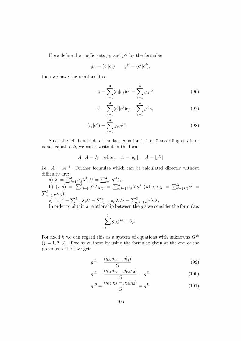
If we define the coefficients gij and gij by the formulae

gij = (ei|ej) gij = (ei|ej),

then we have the relationships:

ei =3∑

j=1

(ei|ej)ej =3∑

j=1

gijej (96)

ei =3∑

j=1

(ei|ej)ej =3∑

j=1

gijej (97)

(ei|ek) =3∑

j=1

gijgjk. (98)

Since the left hand side of the last equation is 1 or 0 according as i is oris not equal to k, we can rewrite it in the form

A · A = I3 where A = [gij], A = [gij]

i.e. A = A−1. Further formulae which can be calculated directly withoutdifficulty are:

a) λi =∑3

j=1 gijλj, λj =

∑3i=1 g

ijλi;

b) (x|y) =∑3

i,j=1 gijλiµj =

∑3i,j=1 gijλ

iµj (where y =∑3

j=1 µjej =

∑3j=1 µ

jej);

c) ‖x‖2 =∑3

i=1 λiλi =

∑3i,j=1 gijλ

iλj =∑3

i,j=1 gijλiλj.

In order to obtain a relationship between the g’s we consider the formulae:

3∑

j=1

gijgjk = δjk.

For fixed k we can regard this as a system of equations with unknowns Gjk

(j = 1, 2, 3). If we solve these by using the formulae given at the end of theprevious section we get:

g11 =(g22g33 − g223)

G(99)

g12 =(g31g32 − g12g33)

G= g21 (100)

g13 =(g12g23 − g22g13)

G= g31 (101)

105

and so on (where G is the determinant of the matrix

g11 g12 g13g21 g22 g23g31 g32 g33

).

Exercises: 1) Calculate the dual bases fora) ((1, 1, 1), (1, 1,−1), (1,−1, 1));b) ((0, 1, 1), (1, 0, 1), (1, 1, 0));c) ((1, 1, 1), (0, 1, 1), (0, 0, 1)) and the corresponding matrices [gij] and

[gij].2) Show that if

x = λ1e1 + λ2e2 + λ3e3 y = µ1e1 + µ2e2 + µ3e3

then the k-th coefficient of x× y with respect to the basis is

3∑

i,j=1

λiµjǫijm

where ǫijk = (ei × ej |ek).3) If x = 2e1 − e2 + 4e3 and y = 2e1 + 3e2 − e3, calculate the coordinates ofx× y with respect to (e1, e2, e3).4) If (e1, e2, e3) is the dual basis to (e1, e2, e3), then

[e1, e2, e3][e1, e2, e3] = 1.

5) If (e1, e2, e3) is a basis, then the set

{x ∈ R3; |(x|ei)| ≤ ‖ei‖ for each i}

is called the Brouillon zone of the unit cell (i.e. the set

{λ1e1 + λ2e2 + λ3e3 : −1 ≤ λi ≤ 1 for each i}).

Calculate it for the following basesa) ((1, 1, 1), (1, 1,−1), (1,−1,−1));b) ((1, 1, 0), (0, 1, 1), (1, 0, 1));c) ((0, 0, 1), (3,−1, 0), (0,−1, 0)).

106

2.10 Isometries of R3

We now analyse the isometries ofR3. We begin by extending some definitionsand results on R2 to R3 in the natural way. A mapping f : R3 → R3 islinear if f(x+y) = f(x)+f(y) and f(λx) = λf(x) for x, y ∈ R3 and λ ∈ R.Then f naps the vector (ξ1, ξ2, ξ3) onto

(a11ξ1 + a12ξ2 + a13ξ3, a21ξ1 + a22ξ2 + a23ξ3, a31ξ1 + a32ξ2 + a33ξ3)

where f(e1) = (a11, a21, a31) etc. The 3× 3 matrix

A =

a11 a12 a13a21 a22 a23a31 a32 a33

is called the matrix of f .If u ∈ R3, Tu denotes the translation operator x 7→ x + u. An affine

mapping f is one of the form tu ◦ f where f is linear. Hence in coordinates,f takes the vector (ξ1, ξ2, ξ3) into the vector

(a11ξ1+a12ξ2+a13ξ3+u1, a21ξ1+a22ξ2+a23ξ3+u2, a31ξ1+a32ξ2+a33ξ3+u3).

A mapping f is an isometry if

‖f(x)− ‖f(y)‖ = ‖x− y‖ (x, y ∈ R3).

If f is linear this is equivalent to the fact that (f(x)|f(y)) = (x|y) for eachx, y. An isometry is automatically affine and if it is linear it maps orthonor-mal bases onto orthonormal bases. (This follows immediately from the factthat (f(xi)|f(xj)) = (xi|xj)). On the other hand, if f is a linear mappingwhich maps one orthonormal basis (x1, x2, x3) onto an orthonormal basis(which we denote by (y1, y2, y3)), then it is an isometry. For if

y = λ1x1 + λ2x2 + λ3x3 y = µ1x1 + µ2x2 + µ3x3,

then (x|y) + λ1µ1 + λ2µ2 + λ3µ3. On the other hand,

f(x) = λ1y1 + λ2y2 + λ3y3 f(y) = µ1y1 + µ2y2 + µ3y3

and so(f(x)|f(y)) = λ1µ1 + λ2µ2 + λ3µ3 = (x|y).

In terms of matrices, we see that f is an isometry if and only if the columnvectors of its matrix A for an orthonormal basis (since they are the imagesof the canonical basis) and this just means that

AtA = I i.e. At = A−1.

107

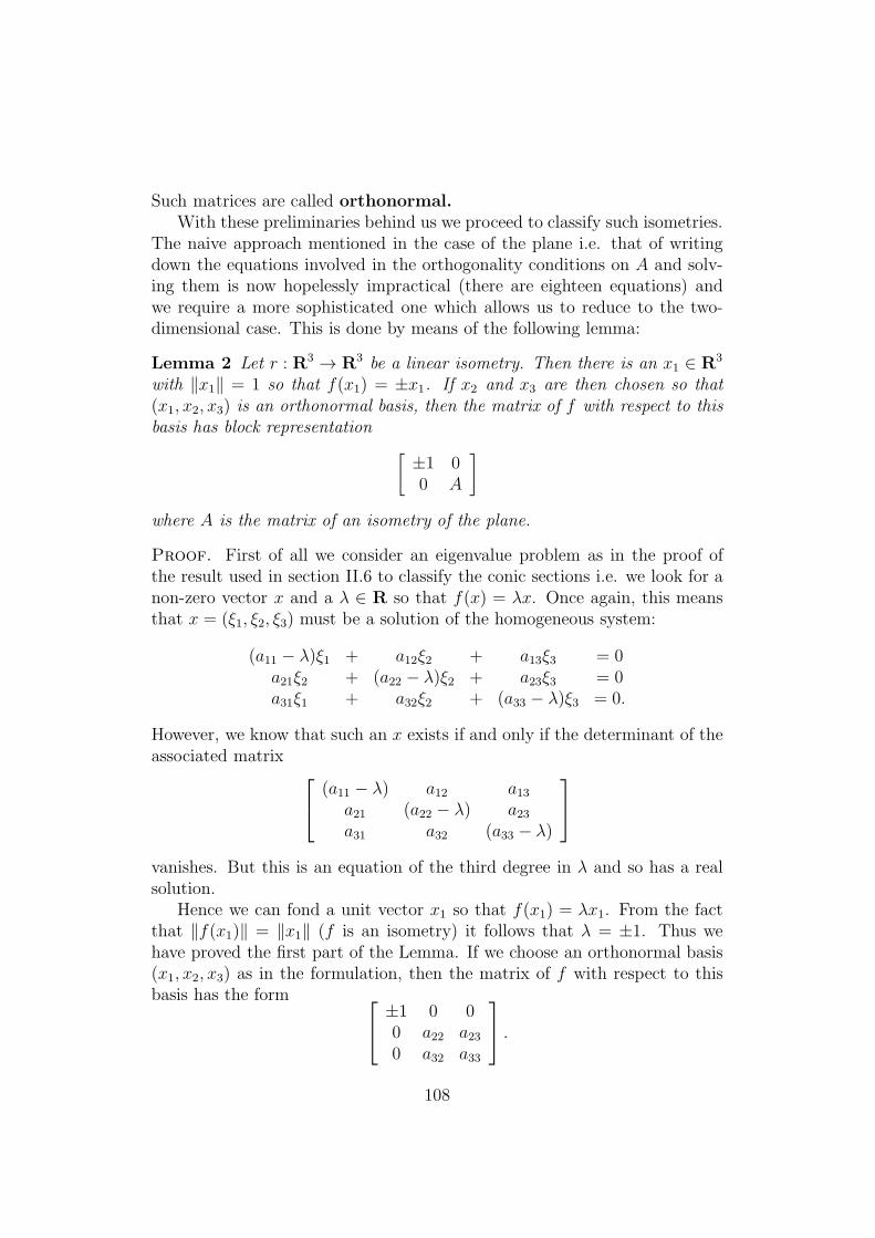
Such matrices are called orthonormal.With these preliminaries behind us we proceed to classify such isometries.

The naive approach mentioned in the case of the plane i.e. that of writingdown the equations involved in the orthogonality conditions on A and solv-ing them is now hopelessly impractical (there are eighteen equations) andwe require a more sophisticated one which allows us to reduce to the two-dimensional case. This is done by means of the following lemma:

Lemma 2 Let r : R3 → R3 be a linear isometry. Then there is an x1 ∈ R3

with ‖x1‖ = 1 so that f(x1) = ±x1. If x2 and x3 are then chosen so that(x1, x2, x3) is an orthonormal basis, then the matrix of f with respect to thisbasis has block representation

[

±1 00 A

]

where A is the matrix of an isometry of the plane.

Proof. First of all we consider an eigenvalue problem as in the proof ofthe result used in section II.6 to classify the conic sections i.e. we look for anon-zero vector x and a λ ∈ R so that f(x) = λx. Once again, this meansthat x = (ξ1, ξ2, ξ3) must be a solution of the homogeneous system:

(a11 − λ)ξ1 + a12ξ2 + a13ξ3 = 0a21ξ2 + (a22 − λ)ξ2 + a23ξ3 = 0a31ξ1 + a32ξ2 + (a33 − λ)ξ3 = 0.

However, we know that such an x exists if and only if the determinant of theassociated matrix

(a11 − λ) a12 a13a21 (a22 − λ) a23a31 a32 (a33 − λ)

vanishes. But this is an equation of the third degree in λ and so has a realsolution.

Hence we can fond a unit vector x1 so that f(x1) = λx1. From the factthat ‖f(x1)‖ = ‖x1‖ (f is an isometry) it follows that λ = ±1. Thus wehave proved the first part of the Lemma. If we choose an orthonormal basis(x1, x2, x3) as in the formulation, then the matrix of f with respect to thisbasis has the form

±1 0 00 a22 a230 a32 a33

.

108

For the equation f(x1) = ±x1 means that the first column is[

±1//0//0]

.

For the second column note that a vector y is in the span of x2 and x3 if andonly if (y|x1) = 0. But then (f(y)|x1) = 0 and the same holds for f(y) (for(z|x1) = 0 implies 0 = (f(y)|f(x1)) = ±(f(y)|x1)). This implies that theremaining two columns of the matrix has the required form. That

[

a22 a23a32 a33

]

is the matrix of an isometry follows from the fact that ‖f(y)‖ = ‖y‖ for eachy of the form η2x2 + η3x3).

We can now classify the linear isometries f on R3. By the above we canchoose an orthonormal basis so that the matrix of f has the form

±1 0 00 a22 a230 a32 a33

where

A =

[

a22 a23a32 a33

]

is the matrix of an isometry in R2. There are four possibilities:1) f(x1) = x1 and A is the matrix of a rotation. Then f is called a rotationabout the axis x1;2) f(x1) = x1 and A is the matrix of a reflection in a line L in the x2, x3-plane. Then f is a reflection in the plane through x1 and L. If wearrange for x2 to be on L then the matrix of f is

1 0 00 1 00 0 −1

and f is reflection in the (x1, x2)-plane;3) f(x1) = −x1 and A is the matrix of a rotation. Then f is a rotation aboutthe x1-axis, followed by a reflection in the plane perpendicular to x1. Suchmappings are called rotary reflections;4) f(x1) = −x1 and A is the matrix of a reflection. In this case we can choosex2 and x3 so that the matrix of f is

−1 0 00 −1 00 0 1

.

109

This is a rotation of 180o about the x3-axis.Summarising, we have proved the following result:

Proposition 22 A linear isometry of R3 has one of the following threeforms:

• rotation;

• a reflection;

• a rotary reflection.

Using this result, we can classify all of the isometries of R3 (including thosewhich are not necessarily linear) as follows:Case a): The isometry f has a fixed point x i.e. is such that f(x) = x.Then if f = T−x ◦ f ◦ Tx, f is a linear isometry. Hence f and so also f is onethe above three types.Case b): As in the two-dimensional case, we put x = f(0) with the resultthat f = Tx ◦ f where f is a linear isometry and so of one of the abovetypes. Hence it suffices to analyses the possible form of such compositions.We relegate this to the following set of exercises and note the results here.There are two new possibilities:

a screw displacement i.e. a mapping of the form Tu ◦ DL,θ where u isparallel to the line L;

a glide reflection i.e. a mapping of the form Tu ◦ RM where u is parallelto the plane M .

Exercises: 1) Give the equation of the following isometries

• a rotation of 60o about the axis (1,−1, 1); item a rotation of 45o aboutthe axis (1, 2, 3);

• a reflection in the two dimensional subspace spanned by the vectors(2, 3, 1) and (1,−1, 1).

Analyse the linear isometries with matrices

0 0 135

−45

045

35

0

resp.

13

23

23

0 1√2

− 1√2

− 43√2

13√2

13√2

.

2) Show that the product RM ◦RM1 of two reflections is

• a rotation about L if the planes meet in the plane L;

110

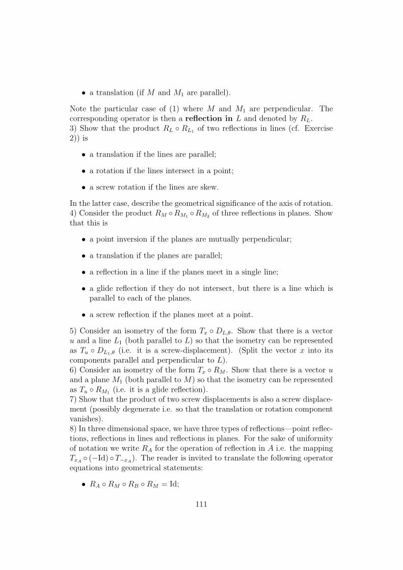
• a translation (if M and M1 are parallel).

Note the particular case of (1) where M and M1 are perpendicular. Thecorresponding operator is then a reflection in L and denoted by RL.3) Show that the product RL ◦ RL1 of two reflections in lines (cf. Exercise2)) is

• a translation if the lines are parallel;

• a rotation if the lines intersect in a point;

• a screw rotation if the lines are skew.

In the latter case, describe the geometrical significance of the axis of rotation.4) Consider the product RM ◦RM1 ◦RM2 of three reflections in planes. Showthat this is

• a point inversion if the planes are mutually perpendicular;

• a translation if the planes are parallel;

• a reflection in a line if the planes meet in a single line;

• a glide reflection if they do not intersect, but there is a line which isparallel to each of the planes.

• a screw reflection if the planes meet at a point.

5) Consider an isometry of the form Tx ◦ DL,θ. Show that there is a vectoru and a line L1 (both parallel to L) so that the isometry can be representedas Tu ◦ DL1,θ (i.e. it is a screw-displacement). (Split the vector x into itscomponents parallel and perpendicular to L).6) Consider an isometry of the form Tx ◦RM . Show that there is a vector uand a plane M1 (both parallel toM) so that the isometry can be representedas Tu ◦RM1 (i.e. it is a glide reflection).7) Show that the product of two screw displacements is also a screw displace-ment (possibly degenerate i.e. so that the translation or rotation componentvanishes).8) In three dimensional space, we have three types of reflections—point reflec-tions, reflections in lines and reflections in planes. For the sake of uniformityof notation we write RA for the operation of reflection in A i.e. the mappingTxA

◦ (−Id) ◦T−xA). The reader is invited to translate the following operator

equations into geometrical statements:

• RA ◦RM ◦RB ◦RM = Id;

111

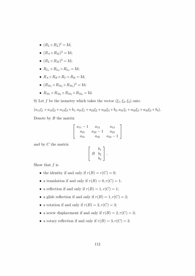
• (RL ◦RL)2 = Id;

• (RA ◦RM)2 = Id;

• (RL ◦RM)2 = Id;

• RL1 ◦RL2 ◦RL3 = Id;

• RA ◦RB ◦RC ◦RB = Id;

• (RM1 ◦RM2 ◦RM3)2 = Id;

• RM1 ◦RM2 ◦RM3 ◦RM4 = Id.

9) Let f be the isometry which takes the vector (ξ1, ξ2, ξ3) onto

(a11ξ1+a12ξ2+a13ξ3+ b1, a21ξ1+a22ξ2+a23ξ3+ b2, a31ξ1+a32ξ2+a33ξ3+ b3).

Denote by B the matrix

a11 − 1 a12 a13a21 a22 − 1 a23a31 a32 a33 − 1

and by C the matrix

b1B b2

b3

.

Show that f is

• the identity if and only if r(B) = r(C) = 0;

• a translation if and only if r(B) = 0, r(C) = 1;

• a reflection if and only if r(B) = 1, r(C) = 1;

• a glide reflection if and only if r(B) = 1, r(C) = 2;

• a rotation if and only if r(B) = 2, r(C) = 3;

• a screw displacement if and only if r(B) = 2, r(C) = 3;

• a rotary reflection if and only if r(B) = 3, r(C) = 3.

112

3 VECTOR SPACES

3.1 The axiomatic definition, linear dependenceand linear combinations

In chapter II we considered the spaces R2 and R3 as models for the two andthree dimensional spaces of our everyday experience and showed how we couldexpress the concepts of geometry in terms of their various structures. Wenow go on to higher dimensional spaces. In the spirit of the previous chapterwe could simply consider the space Rn of n-tuples of real numbers, providedwith the obvious natural operations of addition and scalar multiplication.However, we prefer now to take a more abstract point of view and use theaxiomatic approach whereby we shall introduce vector spaces as sets withstructures which satisfy a variety of properties based on those of R2 and R3.

We shall see that by introducing suitable coordinate systems we can al-ways reduce to the case of the space Rn (and we usually must do this if wewant to calculate concrete examples.) In spite of this fact, the axiomatic orcoordinate-free approach brings several important advantages, not the leastof which are conciseness and elegance of notation and a flexibility in thechoice of coordinate system which can lead to considerable simplification inconcrete calculations.

We begin by introducing the concept of a vector space and develop thelinear part of the programme of the preceding chapter i.e. that part whichdoes not involve the concepts of length, angle and volume. The latter willbe treated in a later chapter.

Definition: A vector space (over R) (or simply a real vector space) isa set V together with an addition and a scalar multiplication i.e. mappingsfrom V × V into V resp. R× V into V written

(x, y) 7→ x+ y resp. (λ, x) 7→ λx

so that

• (x+ y) + z = x+ (y + z) (x, y, z ∈ V );

• x+ y = y + x (x, y ∈ V );

• there exists a zero element i.e. 0 ∈ V so that x + 0 = 0 + x = x forx ∈ V ;

• for each x ∈ V there is an element z ∈ V so that x+ z = z + x = 0;

113

• (λ+ µ)x = λx+ µx (λ, µ ∈ R, x ∈ V );

• λ(x+ y) = λx+ λy (λ ∈ R, x, y ∈ V );

• λ(µx) = (λµ)x (λ, µ ∈ R, x ∈ V );

• 1 · x = x.

We make some simple remarks on these axioms. Firstly, note that thezero element is unique. More precisely, if y ∈ V is such that x + y = x forsome x ∈ V , then y = 0. For if z ∈ V is such that x+ z = 0 (such a z existsby (4)), then z + (x+ y) = z + x = 0 and so (z + x) + y = 0 i.e. 0 + y = 0.Hence y = 0.

Secondly, we have 0 · x = 0 for each x ∈ V . (Here we are guilty of anabuse of notation by using the symbol “0” for the zero element of R and ofthe vector space V ). For x = 1 · x = (1 + 0)x = 1 · x+ 0 · x = x+ 0 · x andso 0 ·x = 0 by the above. Thirdly, the element (−1) ·x has the property of zin (4) i.e. is such that x+ (−1) · x = 0. Hence we denote it by −x and writex− y instead of x+ (−1) · y. Note that (−1) · x is the only element with thisproperty. For if x+ y = 0, then

y = 0 + y = ((−x) + x) + y = (−x) + (x+ y) = (−x) + 0 = −x.

Examples of vector spaces: I. We have already seen that R2 and R3 arevector spaces. In exactly the same way we can regard Rn (the set of n-tuples(ξ1, . . . , ξn) of real numbers) as a vector space by defining

x+ y = (ξ1 + η1, . . . , ξn + ηn) λx = (λξ1, . . . , λξn)

where x = (ξ1, . . . , ξn) and y = (η1, . . . , ηn).II. The set of all n × 1 column vectors i.e. Mn,1 is a vector space with theoperations defined in the first chapter.III. More generally, the set Mm,n of m× n matrices is a vector space.IV. Pol (n), the set of all polynomials of degree at most n, is a vector spaceunder the usual arithmetic operations on functions.V. The space C([0, 1]) of continuous real-valued functions on [0, 1] is also avector space. We will be interested in subsets of vector spaces which arevector spaces in their own right. Of course, this means that they must beclosed under the algebraic operations on V . This leads to the following defi-nition: a subset V1 of a vector space V is a (vector) subspace if wheneverx, y ∈ V1, λ ∈ R, then x+ y ∈ V1 and λx ∈ V1 (a useful reformulation of thiscondition is as follows: whenever x, y ∈ V1, λ, µ ∈ R, then λx+ µy ∈ V1).

114

Examples: The following two subsets

{(ξ1, ξ2, ξ3) ∈ R3 : ξ1 + ξ2 + ξ3 = 0}

{f ∈ C([0, 1]) : f(0) = f(1)}are subspaces of R3 and C([0, 1]) respectively whereas

{(ξ1, ξ2, ξ3) ∈ R3 : ξ1 − ξ2 = 5}

{f ∈ C([0, 1]) :

∫ 1

0

f 2(x) dx = 1}

are not. The notion of dimension played a crucial role in pinpointing thedifference between the plane and space and we shall extend it to generalvector spaces. It is a precise formulation of what is often loosely referred tounder the name of the “number of degrees of freedom”. We shall develop analgebraic characterisation of it, just as we did in R2 and R3.

Definition: A linear combination of the vectors x1, . . . , xm from V is avector of the form λ1x1 + · · · + λmxm for scalars λ1, . . . , λm. The set of allsuch vectors is denoted by [x1, . . . , xm] and is called the space spanned by{x1, . . . , xm}, a name which is justified by the following fact.

Proposition 23 [x1, . . . , xm] is a subspace of V – in fact it is the smallestsubspace containing the vectors x1, . . . , xm.

Proof. If x = λ1x1 + · · · + λmxm and y = µ1x1 + · · · + µmxm are in[x1, . . . , xm], λ ∈ R, then

x+ y = (λ1 + µ1)x1 + · · ·+ (λm + µm)xm

andλx = (λλ1)x1 + · · ·+ (λλm)xm

are also in [x1, . . . , xm] and so the latter is a subspace. On the other hand,if V is a subspace which contains all of the xi, then it clearly contains eachlinear combination thereof and so contains [x1, . . . , xm].

115

Examples: In Pol (5), [1, t, t2] is the set of polynomials of degree at most2 (in other words, Pol (2)) and [t, t2, t3, t4, t5] is the set of polynomials whichvanish at zero.

Continuing with our definitions, we say that a set {x1, . . . , xm} of elementsis linearly independent if only the trivial linear combination 0 ·x1+· · ·+0 ·xm vanishes (in symbols: λ1x1+ · · ·+λmxm = 0 implies λ1 = · · · = λm = 0).As one sees immediately, elements of a linearly independent set must bedistinct and non-zero. Linear dependence (which, of course, is the negationof linear independence) can be characterised thus: the set {x1, . . . , xm} islinearly dependent if and only if at least one of the xi is a linear combinationof the others (for if λ1x1 + · · ·+ λmxm = 0 with say λi 6= 0, then

xi = − 1

λi(λ1x1 + · · ·+ λi−1xi−1 + λi+1xi+1 + . . . λmxm).

We shall sometimes use this fact in the slightly sharper form that if {x1, . . . , xm}is a linearly dependent set, then there is a smallest i so that xi is a linear com-bination of {x1, . . . , xi−1}. To see this simply check the sets {x1}, {x1, x2},{x1, x2, x3},. . . for linear dependence and stop at the first one which is lin-early dependent.

Examples: The set {1, t, t2, . . . , tn} is linearly independent in C([0, 1]) forany n. This is just a restatement of the fact that if a polynomial vanishes on[0, 1] (or, indeed, on any infinite set), then it is the zero polynomial. The set{(1, 0, . . . , 0), (0, 1, 0, . . . , 0), . . . , (0, . . . , 0, 1)} is linearly independent in Rn

as can be seen immediately. We have already encountered the concepts oflinear combination resp. linear independence in the first two chapters (in thecontexts of linear equations and geometry). The latter intuitive approachwill be useful in giving later propositions geometrical content. In actual cal-culations, questions about the linear dependence or independence of concretevectors can be restated in terms of the solvability of systems of linear equa-tions and these can be resolved with the techniques of the first chapter as weshall see below.

116

3.2 Bases (Steinitz’ Lemma)

We are now in a position to define the concept of a basis for a vector space.This is a sequence (x1, . . . , xn) in V so that

• [x1, . . . , xn] = V i.e. the set spans V ;

• {x1, . . . , xn} is linearly independent.

These two conditions mean precisely that every vector x ∈ V has a uniquerepresentation of the form λ1x1 + · · ·+ λnxn. For the first condition ensuresthe existence of such an expansion while the second one guarantees that itis unique.

The λi are then called the coordinates of x with respect to the basis.

Examples: I. The set ((1, 0, . . . , 0), (0, 1, 0, . . . ), . . . , (0, . . . , 0, 1)) is clearlya basis for Rn. Owing to its importance it is called the canonical basis andits elements are denoted by e1, . . . , en.II. More generally, if x1, . . . , xn are elements of Rn and we construct thematrix X whose columns are the vectors x1, . . . , xn (regarded as columnmatrices), then the results of the first chapter can be interpreted as statingthat (x1, . . . , xn) is a basis for Rn if and only if X is invertible.III. The functions (1, t, . . . , tn) form a basis for Pol (n).IV. If we denote by Eij the m × n matrix with a “1” in the (i, j)-th placeand zeroes elsewhere, then the matrices (Eij : 1 ≤ i ≤ m, 1 ≤ j ≤ n) are abasis for Mm,n.

Despite these examples, there do exits vector spaces without bases, oneexample being C([0, 1]). For suppose that this space does have a basis, sayf1, . . . , fn. We choose m > n and express the polynomials tj (j = 1, . . . , m)as linear combinations of the basis, say

tj =n∑

i=1

aijfi (j = 1, . . . , m).

Consider now the equation∑m

j=1 λjtj = 0. This is equivalent to the system

m∑

j=1

aijλj = 0 (i = 1, . . . , n).

Since this is a homogeneous system of n equations in m unknowns, it has anon-trivial solution—which contradicts the linear independence of (1, t, . . . , tm)in C([0, 1]).

117

Notice that we have actually proved that if a vector space V has an infinitesubset, all of whose finite subsets are linearly independent, then V cannothave a basis. Such vector spaces are said to be infinite dimensional. Sincewe shall not be further concerned with such spaces we will tacitly assumethat all spaces are finite dimensional i.e. have (finite) bases.

We shall now prove a number of results on bases which, while beingintuitively rather obvious, are not completely trivial to demonstrate. Thekey to the proofs is the following Lemma which says roughly that a linearlyindependent set spans more space than a linearly dependent one with thesame number of elements.

Proposition 24 Let (x1, . . . , xm) and (y1, . . . , yn) be finite subsets of a vec-tor space V . Suppose that {x1, . . . , xm} is linearly independent and that[x1, . . . , xm] = [y1, . . . , yn]. Then m ≤ n and we can relabel (y1, . . . , yn)as (z1, . . . , zn) so that

[y1, . . . , yn] = [z1, . . . , zn] = [x1, . . . , xm, zm+1, . . . , zn]

i.e. we can successively replace the elements of {z1, . . . , zn} without affectingthe linear span.

Proof. It is convenient to prove the following slight extension of the aboveresult: we show that if 1 ≤ r ≤ m, there is a rearrangement (z1, . . . , zn)(which depends on r) so that

[z1, . . . , zn] = [x1, . . . , xr, zr+1, . . . , zn].

We shall use induction on r.The case r = 1. Since x1 is in the linear span of the yi’s, we have a non-trivialrepresentation

x1 = λ1y1 + · · ·+ λnyn.

Of course, the first coefficient λ1 can vanish. However, by interchanging twoof the yi’s if necessary, we can find a rearrangement (z1, . . . , zn) so that

x1 = µ1z1 + · · ·+ µnzn

with µ1 6= 0. Then[z1, . . . , zn] = [x1, z2, . . . , zn]

since x1 is a linear combination of {x1, z2, . . . , zn}.The step from r to r + 1. There is a rearrangement (z1, . . . , zn) so that

[x1, . . . , xr, zr+1, . . . , zn] = [z1, . . . , zn].

118

Now xr+1 has a representation of the form

µ1x1 + · · ·+ µrxr + µr+1zr+1 + · · ·+ µnzn.

Once again, we can arrange for the coefficient µr+1 to be non-zero (by re-ordering the z’s if necessary). A similar argument now shows that

[x1, . . . , xr+1, zr+2, . . . , zn] = [z1, . . . , zn].

Corollar 1 If a vector space V has two bases (x1, . . . , xm) and (y1, . . . , yn),then m = n.

For it follows immediately from the Lemma that m ≤ n and n ≤ m.Hence if a vector space has a basis, then the number of basis elements is

independent of its choice. We call this number the dimension of V (writtendim V ). Of course, the dimension of Rn is n and we have achieved our firstaim of giving an abstract description of dimension in terms of the vectorspace structure.

Corollar 2 If (x1, . . . , xr) is a linearly independent sequence in an n-dimensionalvector space, then there is a basis of V of the form (x1, . . . , xn) (i.e. we canextend the sequence to a basis for V ).

Proof. Let (y1, . . . , yn) be a basis for V . Applying the Lemma, we get arelabelling (z1, . . . , zn) of the y’s so that (x1, . . . , xr, zr+1, . . . , zn) spans V .This is the required basis.

Corollar 3 If a vector space is spanned by n elements, then it is finite di-mensional and dimV ≤ n.

Corollar 4 Let x1, . . . , xn be elements of a vector space. Then (x1, . . . , xn)is a basis if and only if any two of the following three conditions holds:

• n = dimV ;

• {x1, . . . , xn} is linearly independent;

• {x1, . . . , xn} spans V .

119

In concrete situations, questions about linear dependence and indepen-dence can be settled with the techniques of the first chapter. Suppose thatwe have a sequence (x1, . . . , xn) of vectors in an n-dimensional vector spaceV and wish to determine, for example, the dimension of their linear span[x1, . . . , xn]. We proceed as follows: via a basis we can identify them withrow vectors X1, . . . , Xm in Rn and so define an m× n matrix

A =

X1...Xn

.

We now reduce A to hermitian form A and the required dimension is numberof non-vanishing rows of A i.e. the rank of A.

This method provides the following geometric interpretation of Gaussianelimination: the elementary row operations on the rows of A correspond tothe following operators on the vectors of (x1, . . . , xn):

• exchanging 2 vectors;

• multiplication of xi by a non-zero scalar λ;

• addition of λ times xj to xi.

It is clear that none of these operations affects the linear hull of the set of vec-tors. Thus the method of Gauß can be described as follows: a given sequence(x1, . . . , xn) can be reduced to a linearly independent set (whereby we ignorevanishing vectors) with the same linear span by successive applications ofthe above three elementary operations.

Example: Show that the functions (1 + t, 1− t, 1+ t+ t2) form a basis forPol (2). What are the coordinates of the polynomial α0 + α1t + α2t

2 withrespect to this basis?Solution: First we check the linear independence. The condition

λ(1 + t) + µ(1− t) + ν(1 + t+ t2) = 0

is equivalent to the system

λ+ µ+ ν = 0 (102)

λ− µ+ ν = 0 (103)

ν = 0 (104)

which has only the trivial solution.

120

Similarly, the fact that this linear combination is equal to α0+α1t+α2t2

reduces to the system

λ+ µ+ ν = α0 (105)

λ− µ+ ν = α1 (106)

ν = α2 (107)

with solution λ = 12(α0 + α1 − 2α2), µ = 1

2(α0 − α1), ν = α2.

121

3.3 Complementary subspaces

A useful technique in the theory of vector spaces is that of reducing dimensionby splitting a space into two parts as follows:

Definition: Two subspaces V1 and V2 of a vector space V are said to becomplementary if

• V1 ∩ V2 = {0};

• V = V1 + V2 where the latter denotes the subspace of V consisting ofthose vectors which can be written in the form y + z where y ∈ V1,z ∈ V2.

Then if both of the above conditions hold, each x ∈ V has a unique rep-resentation y + z of the above type (for if y + z = y1 + z1 with y, y1 ∈ V1,z, z1 ∈ V2, then y − y1 = z1 − z and so both sides belong to the intersectionV1 ∩ V2 and must vanish).

V is then said to be split into the two subspaces V1 and V2, a fact whichwe represent symbolically by the equation V = V1 ⊕ V2.

If we have such a splitting, we can construct a basis for V as follows:take bases (x1, . . . , xr) resp. (y1, . . . , ys) for V1 resp. V2. Then the combinedsequence (x1, . . . , xr, y1, . . . , ys) is obviously a basis for V1 ⊕ V2. The sameidea shows how to construct subspaces which are complementary to a givensubspace V1. We simply choose a basis (x1, . . . , xr) for V1 and extend it toa basis (x1, . . . , xn) for V . Then V2 = [xr+1, . . . , xn] is a complementarysubspace. This shows that in general (i.e. except for the trivial case whereV1 = V ), a subspace has many complementary spaces. For example, if V1is a plane in R3 (passing through 0), then any line through 0 which doesnot lie on V1 is complementary. However, regardless of the choice of V2, itsdimension is always n− r and so is determined by V1. This is a special caseof the following result which is useful in dimension counting arguments:

Proposition 25 Let V1 and V2 be subspaces of a vector space V which to-gether span V (i.e. are such that V = V1 + V2). Then

dimV = dimV1 + dimV2 − dim (V1 ∩ V2).

Proof. Note first that V1 ∩ V2 is a subspace of V . Suppose that it hasdimension m and that dimV1 = r, dim V2 = s, dim V = n. We begin with abasis (x1, . . . , xm) for the intersection and extend it to basis

(x1, . . . , xm, xm+1, . . . , xr) for V1

122

and(x1, . . . , xm, x

′m+1, . . . , x

′s) for V2.

We claim that (x1, . . . , xm, . . . , xr, x′m+1, . . . , x

′s) is a basis for V . This suffices

to complete the proof since we then merely have to count the number ofelements in this basis and set it equal to n.

First note that the set spans V since parts of it span V1 and V2 whichin turn span V . Now we shall show that they are linearly independent. Forsuppose that

λ1x1 + · · ·+ λrxr + λm+1x′m+1 + · · ·+ λsx

′s = 0.

Thenλ1x1 + . . . λrxr = −(λm+1x

′m+1 + · · ·+ λsx”s).

Now both sides belong to the intersection and so have a representation ofthe form µ1x1 + · · ·+ µmxm. Equating this to the right hand side of the lastequation above, we get one of the form

µ1x1 + · · ·+ µmxm + λm+1x′m+1 + · · ·+ λsx

′s = 0

and so λm+1 = · · · = λs = 0. This means that the left hand side vanishesand so all of the λ are zero.

123

3.4 Isomorphisms, transfer matrices

Isomorphisms: We have just seen that every vector space V has a basisand this allows us to associate to each vector x ∈ V a set of coordinates(λi). These behave exactly as the ordinary coordinates in Rn with respect toaddition and scalar multiplication. Hence in a certain sense a vector spacewith a basis “is” Rn. In order to make this concept precise, we use thefollowing definition:

Definition: An isomorphism f between vector spaces V and V1 is a bi-jection f from V onto V1 which preserves the algebraic operations i.e. is suchthat

f(x+ y) = f(x) + f(y) f(λx) = λf(x) (x, y ∈ V, λ ∈ R).

V and V1 are then said to be isomorphic. For example, the following spacesare isomorphic: Rn,Mn,1, Pol (n−1). Suitable isomorphism are the mappings

(ξ1, . . . , ξn) 7→

ξ1...ξn

7→ ξ1 + ξ2t+ · · ·+ ξnt

n−1.

We note some simple properties of isomorphisms:

• the identity is an isomorphism and the composition g ◦ f of two iso-morphism is an isomorphism as is the inverse f−1 of an isomorphism;

• isomorphisms respect bases i.e. if f : V → V1 is an isomorphism and(x1, . . . , xn) is a basis for V , then (f(x1), . . . , f(xn)) is a basis for V1.In particular, V and V1 have the same dimension.

In the light of the above remarks and examples, the next result is rathernatural:

Proposition 26 Two vector spaces V and V1 are isomorphic if and only ifthey have the same dimension.

Proof. Suppose that V and V1 have dimension n and choose bases (x1, . . . , xn)resp. (y1, . . . , yn) resp. Then we define a mapping f from V into V1 by setting

f(λ1x1 + · · ·+ λnxn) = λ1y1 + · · ·+ λnyn.

Then f is well-defined because of the uniqueness of the representation of x,injective since the (yi) are linearly independent and surjective since they spanV1. It is clearly linear.

124

In particular, any n-dimensional vector space is isomorphic to Rn, anychoice of basis inducing an isomorphism. Owing to the arbitrariness of sucha choice, we shall require formulae relating the coordinates with respect totwo distinct bases. For example, in R2, the coordinates (λ1, λ2) of the vector(ξ1, ξ2) with respect to the basis ((1, 1), (, 1 − 1)) are the solutions of theequations

λ1 + λ2 = ξ1 (108)

λ1 − λ2 = ξ2 (109)

i.e. λ1 =12(ξ1+ ξ2), λ2 =

12(ξ1− ξ2). Here we recognise the role of the matrix

A =

[

1 11 −1

]

whose columns are the coordinates of the new basis elements. In the generalsituation of bases (x1, . . . , xn) resp. (x

′1, . . . , x

′n) for V , we define the transfer

matrix from (xi) to (x′j) to be the n × n matrix T = [tij ] where the tij aredefined by the equations x′j =

∑ni=1 tijxi i.e. the columns of T are formed by

the coordinates of the x′j with respect to (xi). If x ∈ V has the representation∑n

j=1 λjx′j then, by substituting the above expression for x′j we get

x =n∑

j=1

λ′jx′j =

n∑

j=1

λ′j(n∑

i=1

tijxi) (110)

=

n∑

i=1

(

n∑

j=1

tijλ′j)xi. (111)

Thus we have proved the following result:

Proposition 27 Let T = [tij ] be the transfer matrix from (xi) to (x′j). Thenthe following relationship holds between the coordinates (λ′j) and (λi) of x ∈ Vwith respect to (x′j):

λi =

n∑

j=1

tijλ′j

(i.e. the column matrix of the λ is obtained from that of the λ’-s by multi-plying by the transfer matrix).

If we have to carry our more than one coordinate transformation in the courseof a calculation, the following result is useful:

Proposition 28 Let T (resp. T ′) be the transformation matrix from (xi) to(x′j) resp. from (x′j) to (x′′k). Then the transfer matrix from (xi) to (x′′k) isT · T ′. (Note the order of the factors).

125

Proof. By definition we have

x′j =n∑

i=1

tijxi x′′k =∑

j=1

t′jkx′k.

Hence

x′′k =n∑

j=1

t′jk(n∑

i=1

tijxi) (112)

=

n∑

i=1

(

n∑

j=1

tijt′jk)xi (113)

i.e. t′′ik =∑n

j=1 tijt′jk or T ′′ = T · T ′ where T ′′ = [t′′ik] is the transfer matrix

from (xi) to (x′′k).

Corollar 5 If T is the transfer matrix from (x1, . . . , xn) to (x′1, . . . , x′n), then

its inverse T−1 is the transfer matrix from (x′1, . . . , x′n) to (x1, . . . , xn).

126

3.5 Affine spaces

We conclude this chapter with some remarks on so-called affine spaces. Thereason for introducing these is that the identification of say three dimensionalspace with R3 is based on two arbitrary elements. The first is the choice ofa basis and we have developed methods to deal with this using the transfermatrix between two bases. The second is the choice of the origin or zero ele-ment. This lies rather deeper since it directly involves the algebraic structureof the spaces. This has already manifested itself in the rather inelegant sep-arate treatment that we were forced to give to one (resp. two) dimensionalsubspaces and to lines resp. plane. The way out of this difficulty lies in theconcept of an affine space which we now discuss very briefly.

Definition: An affine space is a set M and a mapping which associatesto each pair (P,Q) in M ×M a vector xPQ in a given vector space V in sucha way that the following conditions hold

• for each P ∈M , the mapping Q 7→ xPQ is a bijection from M onto V ;

• for three points P,Q,R in M we have xPQ + xQR = xPR.

It follows easily from the above conditions thatxPP = 0 for each P ;xPQ = −xQP ;xPQ = xRS implies that xPR = xQS.Of course, there is a very close connection between vector spaces and affine

spaces. Every vector space V is an affine space when we define xPQ = xQ−xPas we did for R3. On the other hand, if M is an affine space and we choosesome point P0 as a zero, then the mapping Q 7→ xP0Q is a bijection from Monto V . We can use it to transfer the vector structure of V to M by definingthe sum of two points Q and Q1 to be that point Q2 for which

xP0Q2 = xP0Q + xP0Q1

and λQ to be that point Q3 for which xP0Q3 = λxP0Q. (In other words, wecan make an affine space into a vector space by arbitrarily promoting oneparticular point to become the zero).

A subset M1 of M is an affine subspace if the set {xPQ : P,Q ∈ M1}is a subspace of V . The dimension of this subspace is then defined to bethe (affine) dimension. We shall give more intrinsic descriptions of theseconcepts shortly. In R3, the zero-dimensional subspaces are the points, theone-dimensional ones are the lines and the two-dimensional ones are planes.

127

Note that a subset M1 of a vector space V (regarded as an affine space asabove) is an affine subspace if and only if it is the translate Tu(V1) of somevector subspace V1 i.e. the set {u+ x : x ∈ V1} for some u ∈ V .

If x0, . . . , xn are points in a vector space V then

M1 = {λ0x0 + · · ·+ λnxn : λ0 . . . , λn ∈ R, λ0 + · · ·+ λn = 1}

is an affine subspace. In fact, it is the smallest such subspace containing thepoints and hence is called the affine subspace generated by them. Forthree non-collinear points in space, this is the plane through these points.One can characterise the above space as Tx0([x1−x0, . . . , xn−x0]) as one seesimmediately. From this representation, one sees that the following conditionsare equivalent:

• dimM1 = n;

• the vectors {x1 − x0, . . . , xn − x0} are linearly independent.

In this case, the vectors {x0, . . . , xn} are said to be affinely independent(note that the apparent special role of x0 is spurious as the equivalence tocondition (1) shows). In this case the λ’s in the representation

λ0x0 + · · ·+ λnxn

(where λ0 + · · · + λn = 1) of a typical element in the affine subspace areuniquely determined. They are called its barycentric coordinates withrespect to x0, . . . , xn. As an example, two points in R3 are affinely indepen-dent if they are distinct, three if they are not collinear. In these cases thebarycentric coordinates coincide with those introduced in Chapter 2.

The signs of the barycentric coordinates determine the position of x withrespect to the faces of the polyhedron with x0, . . . , xn as vertices. Figure 1illustrates the situation for three points in the plane.

Example: a) Is the triple {(1, 3,−1), (3, 0, 1), (1,−1, 1)} linearly indepen-dent? b) Is

[

3 11 −1

]

linearly dependent on

[

1 11 0

]

,

[

1 11 1

]

and

[

0 20 −1

]

?

128

Solution: a) is equivalent to the following: does the system

λ(1, 3,−1) + µ(3, 0, 1) + ν(1,−1, 1) = 0

i.e.λ + 3µ + ν = 03λ − ν = 0−λ + µ + ν = 0

have a non-trivial solution? b) is equivalent to the following: does the system

λ

[

1 11 0

]

+ µ

[

1 11 1

]

+ ν

[

0 20 −1

]

=

[

3 11 −1

]

i.e.λ + µ = 3λ + µ + 2ν = 1λ + µ = 1

µ − ν = −1

have a solution?We leave to the reader the task of answering these questions with the

techniques of Chapter I.

Exercises: 1)

• Which of the following sets of vectors are linearly independent?

(1, 2,−1), (2, 0, 1), (1,−1, 1) (114)

(1,−2, 5, 1), (3, 2, 1,−2), (1, 6,−5,−4) (115)

(1, cos t, sin t). (116)

• For which α are the vectors (α, 1, 0), (1, α, 0), (0, 1, α) linearly indepen-dent?

• Show that the following sets form bases of the appropriate spaces andcalculate the coordinates of the element in brackets with respect to thisbasis:

(1, 1, . . . , 1), (0, 1, . . . , 1), . . . , (0, . . . , 0, 1) in Rn ((ξ1, . . . , ξn)) (117)

1, (t− 1), . . . , (t− 1)n in Pol (n) (a0 + a1t + . . . antn)). (118)

• Calculate the transfer matrix between the following bases:

(x1, x2, x3) and (x1 + x2, x2 + x3, x3 + x1); (119)

(1, t, t2, . . . , tn) and (1, (t− a), . . . , (t− a)n) in Pol (n). (120)

129

• Which of the following subsets of the appropriate vector spaces aresubspaces?

{(ξ1, ξ2, ξ3) ∈ R3 : ξ2 = 0} (121)

{(ξ1, ξ2, ξ3) ∈ R3 : ξ2 > 0} (122)

{(ξ1, ξ2, ξ3) ∈ R3 : ξ21 + ξ22 + ξ23 = 0} (123)

{p ∈ Pol (n) : p(3) = 0} (124)

{p ∈ Pol (n) : p contains only even powers of t} (125)

{A ∈ M2 : aij = aji for each i, j}. (126)

• Calculate the dimensions of the following spaces:

[(1,−2, 1), (−1, 1, 3), (2, 4, 6)] (127)

{(ξ1, ξ2, ξ3) ∈ R3 :

1 0 23 1 −14 1 1

ξ1ξ2ξ3

= 0} (128)

{A ∈Mn : A = At}. (129)

• Show that the following vector space decompositions hold:

R4 = [(1, 0, 1, 0), (1, 1, 0, 0, 0]⊕ [(0, 1, 0, 1), (0, 0, 1, 1)] (130)

R2n = {(ξ1, . . . , ξn, 0, . . . , 0) : (ξ1, . . . , ξn) ∈ Rn} (131)

⊕ {(ξ1, . . . , ξn, ξ1, . . . , ξn) : (ξ1, . . . , ξn) ∈ Rn}. (132)

• What are the dimensions of the following subspaces of Mn?

{A : A is diagonal} (133)

{A : A is upper triangular} (134)

{A : trA = 0}. (135)

2) Show that if V1 and V2 are subspaces of V with V1 ∪ V2 = V , then V1 = Vor V2 = V .3) Let (x1, . . . , xm) be a sequence in V which spans V . Show that it is a basisif there one vector x whose representation is unique. 4) Let V1 be a subspaceof V with dimV1 = dim V . Then V = V1.5) Show that if V , V1 and V2 are subspaces of a given vector space, then

V ∩ V1 + V ∩ V2 ⊂ (V1 + V2) ∩ V (136)

V ∩ (V1 + (V ∩ V2)) = (V ∩ V1) + (V ∩ V1). (137)

130

Show by way of a counterexample that equality does not hold in the firstequation in general.6) Let V1 be a subset of the vector space V . Show that V1 is an affinesubspace of and only if the following condition holds: if x, y ∈ V1, λ ∈ R,then λx+ (1− λ)y ∈ V1.7) Show that if V1 and V2 are subspaces of a given vector space V , then soare V1 ∩ V2 and V1 + V2 where

V1 + V2 = {x+ y : x ∈ V1, y ∈ V2}.

8) Show that the solution space of a system AX = Y is an affine subspace ofRn and that every affine subspaces can be represented in this form. 9) Showthat if V1 and V2 are k-dimensional subspaces of the n dimensional vectorspace V , then they have simultaneous complements i.e. there is a subspaceW of dimension n− k so that

V1 ⊕W = V2 ⊕W = V.

131

4 LINEAR MAPPINGS

4.1 Definitions and examples

In this chapter we introduce the concept of a linear mapping between vectorspaces. We shall see that they are coordinate free versions of matrices, afact which will be useful for two reasons. Firstly, the machinery developed inchapter I will provide us with a method for computing with linear mappingsand secondly this interpretation will provide a useful conceptual frameworkfor our treatment of some more advanced topics in matrix theory. Note thata finite dimensional linear mappings play a central role in mathematics forthe very reason that, while they are simple enough to allow a fairly thoroughanalysis of their properties, they are general enough to have applications inmany branches of mathematics. For while most phenomena which occur innature are described by mappings which are neither finite dimensional norlinear, the standard approach is to approximate such mappings by linear ones(this is the main task of differential calculus) and then these linear ones byfinite dimensional operators (this is an important theme of functional anal-ysis). The solution of the corresponding simplified problem is an importantfirst step in solving the original one (which can be regarded as a perturbedversion of the former).

In fact, we have already met several examples of linear mappings. Inchapter 1 we saw that an m× n matrix A defines a linear mapping betweenspaces of column vectors and in the second chapter we studied linear map-pings in R2 and R3, in particular isometries.

Definition: A mapping f : V → V1 between vector spaces is linear if itsatisfies the following conditions:

• f(x+ y) = f(x) + f(y) (x, y ∈ V );

• f(λx) = λf(x) (λ ∈ R, x ∈ V ).

A simple induction argument shows then that

f(λ1x1 + · · ·+ λnxn) = λ1f(x1) + · · ·+ λnf(xn)

for any n-tuple x1, . . . , xn in V and scalars λ1, . . . , λn.Examples of such mappings areI. Evaluation resp. integration of continuous mappings e.g. the mappings

f 7→f(0) (138)

f 7→∫ 1

0

f(t) dt (139)

132

on C([0, 1]). These can also be regarded as mappings on the spaces Pol (n)of polynomials.II. Formal differentiation and integration of polynomials i.e. the mappings

a0 + a1t+ · · ·+ antn 7→ a1 + 2a2 + · · ·+ nant

n−1 (140)

a0 + a1t+ · · ·+ antn 7→ a0t +

1

2t2 + · · ·+ 1

n+ 1ant

n+1 (141)

from Pol (n) into Pol (n + 1) resp. Pol (n) into Pol (n + 1). (We use theadjective formal to indicate that we are using a purely algebraic definition ofthese operations—in contrast to the general definition, no limiting processesare required in this context).

An important property of linear mappings is the fact that in order tospecify them it suffices to do so on the elements of some bases (xi). For thenthe value of f at x = λ1x1+· · ·+λnxn is automatically λ1f(x1)+· · ·+λnf(xn).

Before studying linear mappings in more detail, we note the fact that ifwe denote by L(V, V1) the set of linear mapping from V into V1, then thisspace has a natural linear structure if we define the algebraic operations inthe obvious way i.e.

(f1 + f2)(x) = f1(x) + f2(x) (142)

(λf)(x) = λf(x). (143)

We shall see later that the dimension of this space is the product of thedimensions of V and V1. In addition, if f : V → V1 and g : V1 → V2 arelinear, then so is the composition g ◦ f : V → V2.

133

4.2 Linear mappings and matrices

Just as in the case of mappings on R2 and R3, matrices in higher dimensionsgenerate linear mappings as follows: if A = [aij ] is an m × n matrix, wedenote by fA the linear mapping

(ξ1, . . . , ξn) 7→ (

n∑

j=1

aijξj)mi=1

from Rn into Rm (this coincides with the fA introduced in the first chapterup to the identification of the set of column vectors with Rn. Hence wealready know that fA is linear). Note that the columns A1, . . . , An of Aare precisely the images of the basis elements e1, . . . , en of Rn (regarded ascolumn vectors).

In fact, using coordinate systems, any linear mapping can be representedby a matrix, as we now show. First we suppose that f maps Rn into Rm

and we define an m× n matrix as above i.e.

A = [aij ] where f(ej) =

m∑

i=1

aijei.

Then f coincides with fA since both agree on the elements of the canonicalbasis). Of course, this construction does not depend on the particular formof the bases and so we can make the following definition:

Definition: Let V and V1 be vector spaces with bases (x1, . . . , xn) resp.(y1, . . . , ym). If f : V → V1 is linear, we define its matrix A with respect to(xi) and (yj) to be the m × n matrix [aij] where the aij are defined by theequations

f(xj) =m∑

i=1

aijyi.

Of course the matrix A depends on the choice of bases and later we shallexamine in detail the effect that a change of basis has on the representingmatrix.

We compute the matrices of some simple operators:I. The matrix of the identity mapping on vector space with respect to anybasis is the unit matrix (of course, we are using the same basis in the rangeand domain space).(x1, . . . , xn) and (x′1, . . . , x

′n) are bases for V , then the matrix of the identity

with respect to (x′j) and (xi) is just the transfer matrix T from (xi) to (x′j)

134

as we see by comparing the above definition with the one of the previouschapter.III. The matrix of the differentiation operator from Pol (n) to Pol (n − 1)with respect to the natural basis is the n× (n+ 1)-matrix

0 1 0 . . . 00 0 2 . . . 0...

...0 0 0 . . . n

.

IV. The matrix of the integral operator from Pol (n) into Pol (n + 1) is the(n + 2)× (n+ 1) matrix

0 0 0 . . . 01 0 0 . . . 00 1

20 . . . 0

......

0 0 0 . . . 1n+1

.

As the following result shows, the algebraic operations for matrices cor-respond to those for linear mappings:

Proposition 29 Let f and f1 be linear mappings from V into V1 resp. ga linear mapping from V1 into V2 where V resp. V1 resp. V2 have bases(x1, . . . , xp) resp. (y1, . . . , yn) resp. (z1, . . . , zm). Denote the correspondingmatrices by Af , Af1 etc. Then

Aλf = λAf Af+f1 = Af + Af1 Ag◦f = AgAf .

Proof. We prove only the last part. Suppose that Af = [ajk] and Ag = [bij ]

i.e.

f(xk) =n∑

j=1

ajkyj g(yj) =m∑

i=1

bijzi.

Then

(g ◦ f)(xk) = g(m∑

j=1

ajkyj) (144)

=∑

ajkg(yj) (145)

=n∑

j=1

ajk(m∑

i=1

bijzi) (146)

=

m∑

i=1

(

n∑

j=1

bijajk)zi (147)

135

i.e. Ag◦f = [∑n

j=1 bijajk]i,k = AgAf .

Of course, this provides further justification for our choice of the definitionof matrix multiplication.

If we apply this result to the case of an operator f : V → V1 where Vhas bases (x1, . . . , xn) and (x′1, . . . , x

′n) resp. V1 has bases (y1, . . . , ym) and

(y′1, . . . , y′m), then we get the following result:

Proposition 30 Let f have matrix A with respect to (x1, . . . , xn) and (y1, . . . , ym)resp. A′ with respect to (x′1, . . . , x

′n) and (y′1, . . . , y

′m). Then we have the re-

lation:A′ = S−1AT

(where S and T are the transfer matrices between the y-bases and the x-basesrespectively).

Proof. We use the fact noted above that T is the matrix of the identityoperator on V with respect to the basis (x′i) into V with the basis (xi). Wenow express f as the product

IdV1 ◦ f ◦ IdV

and read off the corresponding matrices.

Of course, in the case where we are deal with an operator f on a space Vand the x- and y-bases coincide, then the appropriate formula for a changein coordinates is

A′ = T−1AT.

These facts are the motivation for the following definitions (the first oneof which we have already encountered in chapter I):

Definition: Two m × n matrices A and A′ are equivalent if there existinvertible matrices S and T where S is m×m, T is n× n and A′ = S−1AT .This just means that A and A′ are the matrices of the same linear operatorwith respect to different bases.

Two n × n matrices A and A′ are similar if there is an invertible n × nso that A′ = S−1AS. This has a similar interpretation in terms of represen-tations of operators, now with f ∈ L(V ) represented by a single basis.

One of the main tasks of linear algebra is to choose a basis (resp. bases)so that the matrix representing a given operator f has a particularly form(which of the two concepts of equivalence above is appropriate depends on

136

the nature of the problem). For example, the result on matrix equivalencein I.5 can be formulated as follows: every m × n matrix A is equivalent toone of the form

[

Ir 00 0

]

where r = r(A). As a result about linear mappings this says that if f ∈L(V, V1), then there are bases (xj) resp. (yi) for V resp. V1 so that the matrixof f with respect to these bases has the above form (where r = dim f(V )).

It is instructive to give a coordinate free proof of this result. First weintroduce some notation. We consider the subspaces

Kerf = {x ∈ V ; f(x) = 0} Imf = f(V ).

Note that if f is the mapping fA defined by a matrix A then Kerf is theset of solutions of the homogeneous equation AX = 0 and f(V ) is the set ofthose Y for which the equation AX = Y is solvable. In particular, the rankof A is the dimension of Imf . Hence we define the rank r(f) of a generallinear mapping f to be the dimension of the range Imf of f .

Before continuing, we note some simple facts:

• r(f) ≤ dim V and r(f) ≤ dimV1 (for if (x1, . . . , xn) is a basis for V ,then the elements ((f(x1), . . . , f(xn)) span Imf . Hence r(f) ≤ dim V .It is trivial that r(f) ≤ dim (V1).

• if f : V → V1, g : V1 → V2, then

r(g ◦ f) ≤ r(g) and r(g ◦ f) ≤ fr(f).

This follows immediately from (1) since

dim g(f(V )) ≤ dim f(V ) and dim g(f(V )) ≤ dim g(V1).

Note that these correspond to the inequalities r(AB) ≤ r(A) and r(AB) ≤r(B) for matrices which we have already proved.

We now turn to the proof of the representation of a mapping f by amatrix of the form

[

Ir 00 0

]

.

First we choose a basis for Kerf which, for reasons which will soon be ap-parent, we number backwards as (xr+1, . . . , xn). We extend this to a basis(x1, . . . , xr, xr+1, . . . , xn) for V . Let V1 = [x1, . . . , xr] so that Kerf and V1 arecomplementary. Then we claim that f |V1 is an isometry from V1 onto Imf .

137

Proof. It is clear that the mapping is surjective. Suppose that x, y ∈ V1are such that f(x) = f(y). Then x− y is both in V1 and V2 and so vanishessince they are complementary. Hence f is injective on V1.

It then follows that if y1 = f(x1), . . . , yr = f(xr), then (y1, . . . , yr) is abasis for Imf . We extend it to a basis (y1, . . . , ym) for W . Then we see thatthe matrix of f with respect to these bases is of the required form.

From this analysis it is clear that r is just the rank r(f) of f and that

• dim (Kerf) = n− r;

• if dim V = dimW , then the properties of being surjective, injective oran isomorphism for f are equivalent.

Also we have the following splittings:

V = V1 ⊕ V2 W =W1 ⊕W2

where V2 = Ker f,W1 = f(V ), and f |V1 is an isomorphism ontoW1 resp. f |V2

vanishes.We remark that it is often useful to be able to describe the null-space

of a linear mapping f induced by a matrix A explicitly e.g. by specifyinga basis. This can be done with the aid of Gaußian elimination as follows:consider the transposed matrix At and suppose that left multiplication bythe invertible n × n matrix B reduces At to Hermitian form At. Then thelast (n− r) rows of B are a basis for Kerf . This is clear from the equation

BAt = At i.e. ABt = A

which shows that the last (n − r) columns of Bt are annihilated by f . Inother words, they are in the kernel. Of course they are linearly independent(as row of the invertible matrix B) and (n− r) is the dimension of the latter.

If A has block form[

A1 C]

where A1 is a square invertible matrix, then this can be simplified by notingthat the columns of the matrix

[

−A−11 CI

]

form a basis for the kernel of A.If we require a basis for the range of an m × n matrix A then we can

simply take those of its columns which correspond to the pivot elements inthe hermitian form.

138

4.3 Projections and splittings

Projections: An important class of linear mappings are the so-called pro-jections which are defined as follows: let V1 be a subspace of V with comple-mentary subspace V2. Thus every vector x in V has a unique representationof the form y + z (y ∈ V1, z ∈ V2) and we call y the projection of x ontoV1 along V2. This defines a mapping P : x 7→ y form V into V1 which isclearly linear. Any mapping of this form is called a projection.

The following facts follow immediately from the definition:

• P 2 = P ;

• if we construct a basis (xi) for V by combining bases (x1, . . . , xr) forV1 and (xr+1, . . . , xn) for V2, then the matrix of P is

[

Ir 00 0

]

;

• Id− P is the projection of V onto V2 along V1.

In fact, either of the first two properties above characterises projections asthe following result shows:

Proposition 31 If f is a linear operator on the space V then the followingare equivalent:

• f is a projection;

• f is idempotent i.e. f 2 = f ;

• there is a basis (xi) for V with respect to which the matrix of f has theform

[

Ir 00 0

]

.

Then r = r(f) is the dimension of the range of f .

139

Proof. We have already seen that (1) implies (2) and (3). It is clear that(3) implies (2). Hence it remains only to show that (2) implies (1). To dothis we define V1 and V2 to be Im f and Im (Id − f) respectively. Then ifx ∈ V it has a representation f(x) + (x− f(x) as the sum of an element inV1 and one in V2. We shall show that V1 ∩ V2 = {0} and so that V is thedirect sum of V1 and V2. It is then clear that f is the projection onto V1, theimage of f along V2 (the image of Id − f and, simultaneously, the kernel off).

Suppose then that x ∈ V1 ∩ V2. Then x = f(y) for some y ∈ V andx = z − f(z) for some z ∈ V . Then

f(x) = f(z)− f 2(z) = 0

since f is idempotent and

x = f(y) = f 2(y) = f(x) = 0

i.e. x = 0.

The reader should compare the third of the above conditions with theresult that every linear mapping between vector spaces has a matrix of thisform with respect to some choice of bases. Of course, the above conditionis much more restrictive since we are taking the matrix of the operator withrespect to a single basis.

The definition of the splitting of a vector space into a direct sum of twovector subspaces can be generalised to decomposition

V + V1 ⊕ V2 ⊕ · · · ⊕ Vr

of V into such sums of more than two subspaces. This is the case, by defini-tion, if each x ∈ V has a unique representation of the form x1+ · · ·+xr wherexi ∈ Vi. Then we can define operators Pi where Pi(x) = xi (i = 1, . . . , xr).Each Pi is a projection and they satisfy the conditions

• P1 + · · ·+ Pr = Id;

• PiPj = 0(i 6= j).

Such a sequence of projections is called a partition of unity for V . Theycorrespond to decompositions of a basis (x1, . . . , xn) for V into r subbases:

ξ1, . . . , xi1 xi1+1, . . . , xi2 . . . xir−1+1, . . . , xn.

140

Decompositions of the underlying space induce decompositions of linearmappings which correspond to the block representations of matrices discussedin chapter I. For simplicity, we consider the following situation: V has adecomposition V = V1 ⊕ V2, W = W1 ⊕W2 and f is a linear mapping fromV into W . We denote by P1, P2, Q1 and Q2 the projections from V onto V1and V2 resp. from W onto W1 and W2 and define mappings f11 : V1 → W1

etc. where

f11x = Q1f(x) (x ∈ V1); (148)

f12(x) = Q1f(x) (x ∈ V2); (149)

f21(x) = Q2f(x) (x ∈ V1); (150)

f22(x) = Q2f(x) (x ∈ V2). (151)

Then if x = x1 + x2 (x1 ∈ V1, x2 ∈ V2) we see that

f(x) = f(x1) + f(x2) (152)

= (f11(x1) + f12(x2)) + (f21(x1) + f22(x2)) (153)

a fact which can be written symbolically in the form[

f11 f12f21 f22

] [

x1xi2

]

=

[

f11(x1) + f21(x2)f21(x1) + f22(x2)

]

.

If we choose bases (xi) and (yj) for V and W so that (x1, . . . , xs) is a basisfor V1, (xs+1, . . . , xn) is a basis for V2, (y1, . . . , yr) is a basis for W1 and(yr+1, . . . , ym) is a basis for W2, then the matrix of f has the block form

A =

[

A11 A12

A21 A22

]

where Aij is the matrix of fij.We have assembled this apparatus in order to be able to reduce the dimen-

sions in particular computations. This is especially useful in the followingsituations:

• where f(V1) ⊂W1. Then f21 = 0 and the block representation has theform

[

A11 A21

0 A22

]

;

• where f(V1) ⊂W1 and f(V2) ⊂W2. Then the block representation hasthe form

[

A11 00 A22

]

.

141

In most applications V = W , V1 = W1 and V2 = W2. In this case the firstcondition reduces to f(V1) ⊂ V1 in which case we say that V1 is f-invariant.In the second case we have f(V1) ⊂ V1 and f(V2) ⊂ V2 and we say that thesplitting V = V1 ⊕ V2 reduces f .

In this latter case we can reduce questions about f to ones about f11 andf22 which generally brings about great advantages in computations.

142

4.4 Generalised inverses of linear mappings

As we have seen, properties of linear mappings are mirrored in those of ma-trices and vice versa. At this point we shall give a coordinate-free approachto the topic of generalised inverses (cf. I.7). Suppose that f : V → W is alinear operator. We are seeking a linear operator g : W → V so that if theequation f(x) = y has a solution, then x = g(x) is such a solution. We cando this very simply by using the splittings

V = V1 ⊕ V2 W = W1 ⊕W2

constructed in the previous paragraph. Recall that V2 is the kernel of f andW1 is its range. V1 and W2 are arbitrary complementary subspaces. We haveseen that the restriction f of f to V1 is an isomorphism from V1 onto W1. Wedenote its inverse by g and define g to be P ◦ g where P is the projection ofW onto W1 along W2. Then it is easy to check that g is a generalised inversefor f i.e. that the equations

g ◦ f ◦ g = g f ◦ g ◦ f = f

are satisfied. Note also that g ◦ f is the projection onto V1 along V2 whilef ◦ g is the projection onto W1 along W2.

The following two special cases are worth noting separately:

• f is injective. Then Ker f = V2 = {0} and so V = V1. In this case,it is easy to see that g = g ◦ P is a left inverse for f i.e. satisfies theequation g ◦ f = Id. On the other hand, the injectivity of f is clearlynecessary for f to possess a left inverse (for if f is not injective, thenneither is any composition g ◦ f).

• f is surjective. Then W2 = {0}. In this case we can argue in a similarfashion to show that f has a right inverse.

In terms of matrices, these results are restatement of the facts which werediscussed in the first chapter.

143

4.5 Norms and convergence in vector spaces

The theme of convergence of vectors is not properly a part of linear algebra.However, for large systems of equations, the algebraic methods of solutiondescribed in the first chapter are often hopelessly impractical and can be re-placed by iteration methods which provide approximate solutions with muchless effort. The theoretical basis for such methods lies in some simple prop-erties of vector convergence which we now develop.

Definition: A sequence (xn) in Rk converges to x if it converges coordi-natewise i.e. if ξnr → ξr for each r where xn = (ξnr )

kr=1 and x = (ξn).

For practical purposes, it is convenient to specify convergence quantita-tively by means of a so-called norm which is defined as follows:

Definition: A norm on a vector space V is a mapping ‖ ‖ : V → R+ sothat

• ‖x+ y‖ ≤ ‖x‖ + ‖y‖(x, y ∈ V );

• ‖λx‖ = |λ|‖x‖(λ ∈ R, x ∈ V );

• ‖x‖ = 0 implies that x = 0.

The three most commonly used examples of a norm on Rn are as follows:the ℓ1-norm: ‖x‖1 =

∑

i |ξi|; the ℓ2-norm: ‖x‖2 =√∑

i |ξi|2; themaximum norm: ‖x||∞ = maxi |ξi|.

Of course, the ℓ2-norm is exactly the usual euclidean length of the vectorin Rn. All three of these norms induce the convergence described above inthe sense that the sequence (xn) converges to x if and only if the sequenceof norms ‖xn − x|| converges to zero. In fact, it is a general result that allnorms on Rn induce this convergence.

Matrix convergence: In an analogous way, we can define a notion ofconvergence for matrices. A sequence (Ak) ofm×n matrix, where Ak = [akij ],converges to A if akij → aij for each i and j. It follows easily from thisdefinition that if Ak → A and Bk → B, then Ak + Bk → A + B andAkBk → AB.

In practice, convergence of matrices is described by norms of the followingtype. V and V1 are vector spaces with norms ‖ ‖ and ‖ ‖1 respectively. Thenwe define a norm on L(V, V1) as follows:

‖f‖ = sup{‖f(x)‖1 : x ∈ V, ‖x‖ ≤ 1}.

144

This clearly a norm and we have the estimate

‖f(x)‖ ≤ ‖f‖‖x‖ (x ∈ V ).

Note that if f ∈ L(V, V1) and g ∈ L(V1, V2) then the norm of the compositiong ◦ f is at most the product ‖g‖‖f‖. For

‖g ◦ f‖ = sup{‖g(f(x))‖ : ‖x‖ ≤ 1} (154)

≤ ‖g‖ sup{‖f(x)‖ : ‖x‖ ≤ 1} (155)

≤ ‖g‖‖f‖. (156)

In the language of matrices, this means that we have the inequality ‖AB‖ ≤‖A‖‖B‖. We shall use this estimate to prove the following simple fact whichis the basis for many iteration methods for obtaining approximate solutionsfor systems of equations. Suppose that A is an n×n matrix whose norm ‖A‖(with respect to some norm on Rn) is strictly less than 1. Then the series

I − A+ A2 − A3 + · · ·+ (−1)nAn + . . .

converges and its sum is an inverse for the matrix I + A. (In particular, weare claiming that the latter is invertible). In order to prove the convergenceone apes the proof of the fact that the geometric series converges if |a| < 1.One then multiplies out the partial sums to get the equations

(I + A)Sn = Sn(I + A) = I − An+1

where Sn =∑n

r=0(−1)rAr. Now ‖An+1‖ ≤ ‖A‖n+1 by a repeated used of theinequality for the norm of a product and so the right hand side converges toI from which it follows that the limit of the sequence (Sn) is an inverse forI + A.

This can be used to give an iterative method for solving the equationBX = Y where B is a matrix of the form I+A with ‖A‖ < 1 for some normon Rn. By the above, the solution is

X = (I + A)−1Y = Y − AY + A2Y − A3Y + . . . .

This can be most conveniently implemented with the following scheme. Onechooses an initial value X0 for the solution and defines a sequence (Xn) ofvectors iteratively by means of the formula Xn+1 = Y − AXn. Then thevectors Xn converge to the solution of the equation. For if we substitutesuccessively in the defining equations for Xn we see that

X1 = Y − AX0 (157)

X2 = Y − AY + A2X0 (158)

... (159)

xin = (I −A + A2 − · · ·+ (−1)n−1An−1)Y ± AnX0. (160)

145

In order to be able to apply this method, we require estimates for thenorms of matrices with respect to suitable norms on Rn. We note here thatfor the cases of ‖ ‖1 and ‖ ‖∞, we have the exact formulae:

‖A‖ = maxj

∑

i

|aij | (161)

‖A‖∞ = maxi

∑

j

|aij | (162)

(see the exercises below).

Example: Consider the equation BX = Y where B is an n × n matrixwhich is dominated by its diagonal in the sense that

|bii| >∑

j 6=i

|bij |

for each i. Then we can splitB into the sumD+B1 whereD = diag (b11, . . . , bnn)and

B1 =

0 b12 . . . b1nb21 0 . . . b2n...

...bn1 bn2 . . . 0

.

The equation can now be written in the form

D−1BX = D−1Y

and the matrix D−1B has the form I + A where the norm of A is less than1. Hence we can apply the above to obtain the following method of solution.We choose a suitable approximation X0 to the solution and use the formula

Xn+1 = D−1(Y −B1Xn)

to define recursively a sequence of vectors which converges to the exact so-lution.

Similar considerations lead to the following iterative method for deter-mining approximations to the inverse of a matrix A. We start off with areasonable approximation D to the inverse. How far away this is from beingan inverse is described by the difference C = I−DA. We assume that this issmall in the sense that has norm less than one for some norm on Rn. Then

146

we use the iteration scheme

D1 = D(I + C) (163)

C1 = I −AD1 (164)

D2 = D1(I + C1) (165)

C2 = I −AD2 (166)

and so on. The resulting sequence (Dn) converges to the inverse of A.

Exercises 1)

• Consider the mapping

(ξ1, ξ2) 7→ (ξ1 + 3ξ2, 3ξ1 + ξ2).

Calculate its matrix with respect to the following pairs of bases:

((1, 0), 0, 1)) and ((1, 1), (1,−1)); (167)

((1, 1), (1,−1)) and ((1, 0), (0, 1)); (168)

((1, 1), (1,−1)) and ((1, 1), (1,−1)). (169)

• Calculate the matrix of the mapping

(ξ1, ξ2, ξ3) 7→ (2ξ2 + ξ3, ξ1 + ξ2 + ξ3, ξ1 − ξ2).

• Calculate the matrix of the mappings

p 7→ (t 7→ (p(t− 1)− p(t)) (170)

p 7→ (t 7→ p(t+ 1)) (171)

with respect to the canonical basis of Pol (n).

• Calculate the kernel and the range of the mapping f which takes(ξ1, ξ2, ξ3, ξ4) onto the vector

(ξ1 + ξ2 − ξ3 + ξ4, ξ2 − ξ3, 6ξ1 + 2ξ2 − 3ξ3 + 4ξ4).

• Calculate the matrix of the projection onto [(1, 0, 1), (0,−1, 0)] along[(2, 2, 2)] with respect to the canonical basis.

• Calculate the image of the corners (±1,±1,±1) of the cube under theprojection onto the plane

{(ξ1, ξ2, ξ3); ξ1 + ξ2 + ξ3 = 0}

along (1, 1, 1).

147

• Find the matrix of the mapping A 7→ AB (where B is a fixed 2 × 2matrix) with respect to the basis

[

1 00 0

] [

0 10 0

] [

0 01 0

] [

0 00 1

]

.

2) Calculate the matrix of the operator∑n

i=1 aiDn on Pol (n). For which

values of the ai is it invertible? Calculate the inverse in the case where

ai =1

i!.

3) For which f ∈ L(V ) does there exist a g ∈ L(V ) wo that g ◦ f = 0 (withg non-zero).4) Let V1 (resp. W1) be a subspace of V (resp. W ) so that

dim V1 + dim W1 = dim V.

Show that there is a linear mapping f from V into W so that V1 = Ker f ,W1 = f(V1).5) Show that if f ∈ L(V ), then there is a polynomial p so that p(f) = 0(where if p(t) = a0 + a1t + · · ·+ art

r, then p(f) = a0Id + a1f + · · ·+ arfr).

Deduce that if f is invertible, then there is a polynomial p so that f−1 = p(f).6) Let p1, p2 be projections in L(V ). Show that

p1 + p2 is a projection if and only if p1p2 = p2p1 = 0;p1 − p2 is a projection if and only if p1p2 = p2p1 = p2; indent p1p2 is a

projection if and only if p1p2 = p2p1.Interpret these statements geometrically and describe the ranges of the cor-responding projections in terms of those of p1 and p2.

If p is a projection onto the subspace V1 of V and f ∈ L(V ), show thatf(V1) ⊂ V1 if and only if pfp = fp. For which f is the condition fp = pfsatisfied?7) Calculate the matrix of the differentiation operator on the space of con-tinuous functions spanned by

{eλt, teλt, . . . , tneλt}

(with these functions as basis).8) Verify the above formulae for the norm of A with respect to ‖ ‖1 respec-tively ‖ ‖∞.9) A norm ‖ ‖ on Rn is monotonic if ‖x‖ ≤ ‖y‖ whenever |ξi| ≤ |ηi| foreach i. Show that if D is the diagonal matrix diag (λ1, . . . , λn), then theassociated norm of D for a monotonic norm is

max(|λ1|, . . . , |λn|).

148

10) (The following is a particular example of a method for calculating certainindefinite integrals of classical functions). Denote by V the two dimensionalvector space generated by the functions

x(t) = eat cos bt, y(t) = eat sin bt.

Note that the operation of differentiation maps V into itself and calculateits matrix with respect to the basis (x, y). Use the inverse of this matrixto calculate the indefinite integrals of x and y. (This works for any finitedimensional vector spaces of suitable differentiable functions which do notcontain the constants and are invariant under differentiation. The reader isinvited to construct further examples).11) Suppose that M is a subset of the space L(V ) of linear operators on thevector space V . Show that if the only subspaces of V which are invariantunder each f in M are {0} and V itself, then an operator g which commuteswith each element of M is either 0 or is invertible.

149