Linear Algebra II (MAT 3141) - Alistair Savage 3141 - Linear... · 2016-05-26 · Linear Algebra II...
243
Linear Algebra II (MAT 3141) Course notes written by Damien Roy with the assistance of Pierre Bel and financial support from the University of Ottawa for the development of pedagogical material in French (Translated into English by Alistair Savage) Fall 2012 Department of Mathematics and Statistics University of Ottawa
Transcript of Linear Algebra II (MAT 3141) - Alistair Savage 3141 - Linear... · 2016-05-26 · Linear Algebra II...

Linear Algebra II (MAT 3141)
Course notes written by Damien Roy
with the assistance of Pierre Bel
and financial support from the University of Ottawa
for the development of pedagogical material in French
(Translated into English by Alistair Savage)
Fall 2012
Department of Mathematics and Statistics
University of Ottawa

Contents
Preface v
1 Review of vector spaces 1
1.1 Vector spaces . . . . . . . . . . . . . . . . . . . . . . . . . . . . . . . . . . . 1
1.2 Vector subspaces . . . . . . . . . . . . . . . . . . . . . . . . . . . . . . . . . 3
1.3 Bases . . . . . . . . . . . . . . . . . . . . . . . . . . . . . . . . . . . . . . . . 4
1.4 Direct sum . . . . . . . . . . . . . . . . . . . . . . . . . . . . . . . . . . . . . 7
2 Review of linear maps 13
2.1 Linear maps . . . . . . . . . . . . . . . . . . . . . . . . . . . . . . . . . . . . 13
2.2 The vector space LK(V,W ) . . . . . . . . . . . . . . . . . . . . . . . . . . . 16
2.3 Composition . . . . . . . . . . . . . . . . . . . . . . . . . . . . . . . . . . . . 18
2.4 Matrices associated to linear maps . . . . . . . . . . . . . . . . . . . . . . . 21
2.5 Change of coordinates . . . . . . . . . . . . . . . . . . . . . . . . . . . . . . 24
2.6 Endomorphisms and invariant subspaces . . . . . . . . . . . . . . . . . . . . 26
3 Review of diagonalization 33
3.1 Determinants and similar matrices . . . . . . . . . . . . . . . . . . . . . . . 33
3.2 Diagonalization of operators . . . . . . . . . . . . . . . . . . . . . . . . . . . 36
3.3 Diagonalization of matrices . . . . . . . . . . . . . . . . . . . . . . . . . . . . 41
4 Polynomials, linear operators and matrices 47
4.1 The ring of linear operators . . . . . . . . . . . . . . . . . . . . . . . . . . . 47
4.2 Polynomial rings . . . . . . . . . . . . . . . . . . . . . . . . . . . . . . . . . 48
4.3 Evaluation at a linear operator or matrix . . . . . . . . . . . . . . . . . . . . 54
5 Unique factorization in euclidean domains 59
5.1 Divisibility in integral domains . . . . . . . . . . . . . . . . . . . . . . . . . 59
5.2 Divisibility in terms of ideals . . . . . . . . . . . . . . . . . . . . . . . . . . . 62
5.3 Euclidean division of polynomials . . . . . . . . . . . . . . . . . . . . . . . . 64
5.4 Euclidean domains . . . . . . . . . . . . . . . . . . . . . . . . . . . . . . . . 65
5.5 The Unique Factorization Theorem . . . . . . . . . . . . . . . . . . . . . . . 69
5.6 The Fundamental Theorem of Algebra . . . . . . . . . . . . . . . . . . . . . 72
i

ii CONTENTS
6 Modules 756.1 The notion of a module . . . . . . . . . . . . . . . . . . . . . . . . . . . . . . 756.2 Submodules . . . . . . . . . . . . . . . . . . . . . . . . . . . . . . . . . . . . 806.3 Free modules . . . . . . . . . . . . . . . . . . . . . . . . . . . . . . . . . . . 836.4 Direct sum . . . . . . . . . . . . . . . . . . . . . . . . . . . . . . . . . . . . . 846.5 Homomorphisms of modules . . . . . . . . . . . . . . . . . . . . . . . . . . . 86
7 The structure theorem 917.1 Annihilators . . . . . . . . . . . . . . . . . . . . . . . . . . . . . . . . . . . . 917.2 Modules over a euclidean domain . . . . . . . . . . . . . . . . . . . . . . . . 997.3 Primary decomposition . . . . . . . . . . . . . . . . . . . . . . . . . . . . . . 1027.4 Jordan canonical form . . . . . . . . . . . . . . . . . . . . . . . . . . . . . . 108
8 The proof of the structure theorem 1198.1 Submodules of free modules, Part I . . . . . . . . . . . . . . . . . . . . . . . 1198.2 The Cayley-Hamilton Theorem . . . . . . . . . . . . . . . . . . . . . . . . . 1248.3 Submodules of free modules, Part II . . . . . . . . . . . . . . . . . . . . . . . 1278.4 The column module of a matrix . . . . . . . . . . . . . . . . . . . . . . . . . 1308.5 Smith normal form . . . . . . . . . . . . . . . . . . . . . . . . . . . . . . . . 1348.6 Algorithms . . . . . . . . . . . . . . . . . . . . . . . . . . . . . . . . . . . . . 141
9 Duality and the tensor product 1559.1 Duality . . . . . . . . . . . . . . . . . . . . . . . . . . . . . . . . . . . . . . . 1559.2 Bilinear maps . . . . . . . . . . . . . . . . . . . . . . . . . . . . . . . . . . . 1609.3 Tensor product . . . . . . . . . . . . . . . . . . . . . . . . . . . . . . . . . . 1669.4 The Kronecker product . . . . . . . . . . . . . . . . . . . . . . . . . . . . . . 1729.5 Multiple tensor products . . . . . . . . . . . . . . . . . . . . . . . . . . . . . 176
10 Inner product spaces 17910.1 Review . . . . . . . . . . . . . . . . . . . . . . . . . . . . . . . . . . . . . . . 17910.2 Orthogonal operators . . . . . . . . . . . . . . . . . . . . . . . . . . . . . . . 18610.3 The adjoint operator . . . . . . . . . . . . . . . . . . . . . . . . . . . . . . . 19010.4 Spectral theorems . . . . . . . . . . . . . . . . . . . . . . . . . . . . . . . . . 19310.5 Polar decomposition . . . . . . . . . . . . . . . . . . . . . . . . . . . . . . . 199
Appendices 205
A Review: groups, rings and fields 207A.1 Monoids . . . . . . . . . . . . . . . . . . . . . . . . . . . . . . . . . . . . . . 207A.2 Groups . . . . . . . . . . . . . . . . . . . . . . . . . . . . . . . . . . . . . . . 209A.3 Subgroups . . . . . . . . . . . . . . . . . . . . . . . . . . . . . . . . . . . . . 212A.4 Group homomorphisms . . . . . . . . . . . . . . . . . . . . . . . . . . . . . . 213A.5 Rings . . . . . . . . . . . . . . . . . . . . . . . . . . . . . . . . . . . . . . . . 215A.6 Subrings . . . . . . . . . . . . . . . . . . . . . . . . . . . . . . . . . . . . . . 219A.7 Ring homomorphisms . . . . . . . . . . . . . . . . . . . . . . . . . . . . . . . 220A.8 Fields . . . . . . . . . . . . . . . . . . . . . . . . . . . . . . . . . . . . . . . 222

CONTENTS iii
B The determinant 223B.1 Multilinear maps . . . . . . . . . . . . . . . . . . . . . . . . . . . . . . . . . 223B.2 The determinant . . . . . . . . . . . . . . . . . . . . . . . . . . . . . . . . . 228B.3 The adjugate . . . . . . . . . . . . . . . . . . . . . . . . . . . . . . . . . . . 231

iv CONTENTS

Preface
These notes are aimed at students in the course Linear Algebra II (MAT 3141) at theUniversity of Ottawa. The first three chapters contain a revision of basic notions coveredin the prerequisite course Linear Algebra I (MAT 2141): vector spaces, linear maps anddiagonalization. The rest of the course is divided into three parts. Chapters 4 to 8 make upthe main part of the course. They culminate in the structure theorem for finite type modulesover a euclidean ring, a result which leads to the Jordan canonical form of operators on afinite dimensional complex vector space, as well as to the structure theorem for abeliangroups of finite type. Chapter 9 involves duality and the tensor product. Then Chapter 10treats the spectral theorems for operators on an inner product space (after a review of somenotions seen in the prerequisite course MAT 2141). With respect to the initial plan, theystill lack an eleventh chapter on hermitian spaces, which will be added later. The notes arecompleted by two appendices. Appendix A provides a review of basic algebra that are usedin the course: groups, rings and fields (and the morphisms betwen these objects). AppendixB covers the determinants of matrices with entries in an arbitrary commutative ring andtheir properties. Often the determinant is simply defined over a field and the goal of thisappendix is to show that this notion easily generalizes to an arbitrary commutative ring.
This course provides students the chance to learn the theory of modules that is notcovered, due to lack of time, in other undergraduate algebra courses. To simplify mattersand make the course easier to follow, I have avoided introducing quotient modules. This topiccould be added through exercises (for more motivated students). According to comments Ihave received, students appreciate the richness of the concepts presented in this course andthat they open new horizons to them.
I thank Pierre Bel who greatly helped with the typing and updating of these notes. I alsothank the Rectorat aux Etudes of the University of Ottawa for its financial support of thisproject via the funds for the development of French teaching materials. This project wouldnot have been possible without their help. Finally, I thank my wife Laura Dutto for her helpin the revision of preliminary versions of these notes and the students who took this coursewith me in the Winter and Fall of 2009 for their participation and their comments.
Damien Roy (as translated by Alistair Savage) Ottawa, January 2010.
v

Chapter 1
Review of vector spaces
This chapter, like the two that follow it, is devoted to a review of fundamental conceptsof linear algebra from the prerequisite course MAT 2141. This first chapter concerns themain object of study in linear algebra: vector spaces. We recall here the notions of a vectorspace, vector subspace, basis, dimension, coordinates, and direct sum. The reader shouldpay special attention to the notion of direct sum, since it will play a vital role later in thecourse.
1.1 Vector spaces
Definition 1.1.1 (Vector space). A vector space over a field K is a set V with operations ofaddition and scalar multiplication:
V × V −→ V(u,v) 7−→ u + v
andK × V −→ V(a,v) 7−→ av
that satisfies the following axioms:
VS1. u + (v + w) = (u + v) + wVS2. u + v = v + u
}for all u,v,w ∈ V.
VS3. There exists 0 ∈ V such that v + 0 = v for all v ∈ V .VS4. For all v ∈ V , there exists −v ∈ V such that v + (−v) = 0.
VS5. 1v = vVS6. a(bv) = (ab)vVS7. (a+ b)v = av + bvVS8. a(u + v) = au + av
for all a, b ∈ K and u,v ∈ V .
These eight axioms can be easily interpreted. The first four imply that (V,+) is anabelian group (cf. Appendix A). In particular, VS1 and VS2 imply that the order in which
1

2 CHAPTER 1. REVIEW OF VECTOR SPACES
we add the elements v1, . . . ,vn of V does not affect their sum, denoted
v1 + · · ·+ vn orn∑i=1
vi.
Condition VS3 uniquely determines the element 0 of V . We call it the zero!vector of V ,the term vector being the generic name used to designate an element of a vector space. Foreach v ∈ V , there exists one and only one vector −v ∈ V that satisfies VS4. We call it theadditive inverse of v. The existence of the additive inverse allows us to define subtractionin V by
u− v := u + (−v).
Axioms VS5 and VS6 involve only scalar multiplication, while the Axioms VS7 andVS8 link the two operations. These last axioms require that multiplication by a scalar bedistributive over addition on the right and on the left (i.e. over addition in K and in V ).They imply general distributivity formulas:(
n∑i=1
ai
)v =
n∑i=1
aiv and an∑i=1
vi =n∑i=1
avi
for all a, a1, . . . , an ∈ K and v,v1, . . . ,vn ∈ V .
We will return to these axioms later when we study the notion of a module over acommutative ring, which generalizes the idea of a vector space over a field.
Example 1.1.2. Let n ∈ N>0. The set
Kn =
a1
a2...an
; a1, a2, . . . , an ∈ K
of n-tuples of elements of K is a vector space over K for the operations:
a1
a2...an
+
b1
b2...bn
=
a1 + b1
a2 + b2...
an + bn
and c
a1
a2...an
=
c a1
c a2...
c an
.
In particular, K1 = K is a vector space over K.
Example 1.1.3. More generally, let m,n ∈ N>0. The set
Matm×n(K) =
a11 · · · a1n
......
am1 . . . amn
; a11, . . . , amn ∈ K

1.2. VECTOR SUBSPACES 3
of m× n matrices with entries in K is a vector space over K for the usual operations:
a11 · · · a1n...
...am1 . . . amn
+
b11 · · · b1n...
...bm1 . . . bmn
=
a11 + b11 · · · a1n + b1n...
...am1 + bm1 . . . amn + bmn
and c
a11 · · · a1n...
...am1 . . . amn
=
c a11 · · · c a1n...
...c am1 . . . c amn
.
Example 1.1.4. Let X be an arbitrary set. The set F(X,K) of functions from X to K is avector space over K when we define the sum of two functions f : X → K and g : X → K tobe the function f + g : X → K given by
(f + g)(x) = f(x) + g(x) for all x ∈ X,
and the product of f : X → K and a scalar c ∈ K to be the function c f : X → K given by
(c f)(x) = c f(x) for all x ∈ X.
Example 1.1.5. Finally, if V1, . . . , Vn are vector spaces over K, their cartesian product
V1 × · · · × Vn = {(v1, . . . ,vn) ; v1 ∈ V1, . . . ,vn ∈ Vn}
is a vector space over K for the operations
(v1, . . . ,vn) + (w1, . . . ,wn) = (v1 + w1, . . . ,vn + wn),
c(v1, . . . ,vn) = (cv1, . . . , cvn).
1.2 Vector subspaces
Fix a vector space V over a field K.
Definition 1.2.1 (Vector subspace). A vector subspace of V is a subset U of V satisfying thefollowing conditions:
SUB1. 0 ∈ U.SUB2. If u,v ∈ U, then u + v ∈ U.SUB3. If u ∈ U and c ∈ K, then cu ∈ U.
Conditions SUB2 and SUB3 imply that U is stable under the addition in V and stableunder scalar multiplication by elements of K. We thus obtain the operations
U × U −→ U(u,v) 7−→ u + v
andK × U −→ U(a,v) 7−→ av
on U and we see that, with these operations, U is itself a vector space. Condition SUB1can be replaced by U 6= ∅ because, if U contains an element u, then SUB3 implies that0 u = 0 ∈ U . Nevertheless, it is generally just as easy to verify SUB1. We therefore havethe following proposition.

4 CHAPTER 1. REVIEW OF VECTOR SPACES
Proposition 1.2.2. A vector subspace U of V is a vector space over K for the addition andscalar multiplication restricted from V to U .
We therefore see that all vector subspaces of V give new examples of vector spaces. IfU is a subspace of V , we can also consider subspaces of U . However, we see that these aresimply subspaces of V contained in U . Thus, this does not give new examples. In particular,the notion of being a subspace is transitive.
Proposition 1.2.3. If U is a subspace of V and W is a subspace of U , then W is a subspaceof V .
We can also form the sum and intersection of subspaces of V :
Proposition 1.2.4. Let U1, . . . , Un be subspaces of V . The sets
U1 + · · ·+ Un = {u1 + · · ·+ un ; u1 ∈ U1, . . . ,un ∈ Un} and
U1 ∩ · · · ∩ Un = {u ; u ∈ U1, . . . ,u ∈ Un} ,
called, respectively, the sum and intersection of U1, . . . , Un, are subspaces of V .
Example 1.2.5. Let V1 and V2 be vector spaces over K. Then
U1 = V1 × {0} = {(v1,0) ; v1 ∈ V1} and U2 = {0} × V2 = {(0,v2) ; v2 ∈ V2}
are subspaces of V1 × V2. We see that
U1 + U2 = V1 × V2 and U1 ∩ U2 = {(0,0)} .
1.3 Bases
In this section, we fix a vector space V over a field K and elements v1, . . . ,vn of V .
Definition 1.3.1 (Linear combination). We say that an element v of V is a linear combinationof v1, . . . ,vn if there exist a1, . . . , an ∈ K such that
v = a1v1 + · · ·+ anvn.
We denote by〈v1, . . . ,vn〉K = {a1v1 + · · ·+ anvn ; a1, . . . , an ∈ K}
the set of linear combinations of v1, . . . ,vn. This is also sometimes denoted SpanK{v1, . . . ,vn}.
The identities0v1 + · · ·+ 0vn = 0n∑i=1
aivi +n∑i=1
bivi =n∑i=1
(ai + bi)vi
cn∑i=1
aivi =n∑i=1
(c ai)vi

1.3. BASES 5
show that 〈v1, . . . ,vn〉K is a subspace of V . This subspaces contains v1, . . . ,vn since we have
vj =n∑i=1
δi,jvi where δi,j =
{1 if i = j,0 otherwise.
Finally, every subspace of V that contains v1, . . . ,vn also contains all linear combinations ofv1, . . . ,vn, that is, it contains 〈v1, . . . ,vn〉K . Therefore:
Proposition 1.3.2. The set 〈v1, . . . ,vn〉K of linear combinations of v1, . . . ,vn is a subspaceof V that contains v1, . . . ,vn and that is contained in all subspaces of V containing v1, . . . ,vn.
We express this property by saying that 〈v1, . . . ,vn〉K is the smallest subspace of V thatcontains v1, . . . ,vn (with respect to inclusion). We call it the subspace of V generated byv1, . . . ,vn.
Definition 1.3.3 (Generators). We say that v1, . . . ,vn generates V or that {v1, . . . ,vn} is asystem of generators (or generating set) of V if
〈v1, . . . ,vn〉K = V
We say that V is a subspace of finite type (or is finite dimensional) if it admits a finitesystem of generators.
It is important to distinguish the finite set {v1, . . . ,vn} consisting of n elements (count-ing possible repetitions) from the set 〈v1, . . . ,vn〉K of their linear combinations, which isgenerally infinite.
Definition 1.3.4 (Linear dependence and independence). We say that the vectors v1, . . . ,vnare linearly independent , or that the set {v1, . . . ,vn} is linearly independent if the only choiceof a1, . . . , an ∈ K such that
a1v1 + · · ·+ anvn = 0 (1.1)
is a1 = · · · = an = 0. Otherwise, we say that the vectors v1, . . . ,vn are linearly dependent .
In other words, v1, . . . ,vn are linearly dependent if there exist a1, . . . , an, not all zero,that satisfy Condition (1.1). A relation of the form (1.1) with a1, . . . , an not all zero is calleda linear dependence relation among v1, . . . ,vn.
Definition 1.3.5 (Basis). We say that {v1, . . . ,vn} is a basis of V if {v1, . . . ,vn} is a systemof linearly independent generators for V .
The importance of the notion of basis comes from the following result:
Proposition 1.3.6. Suppose that {v1, . . . ,vn} is a basis for V . For all v ∈ V , there existsa unique choice of scalars a1, . . . , an ∈ K such that
v = a1v1 + · · ·+ anvn . (1.2)

6 CHAPTER 1. REVIEW OF VECTOR SPACES
Proof. Suppose v ∈ V . Since the vectors v1, . . . ,vn generate V , there exist a1, . . . , an ∈ Ksatisfying (1.2). If a′1, . . . , a
′n ∈ K also satisfy v = a′1v1 + · · ·+ a′nvn, then we have
0 = (a1v1 + · · ·+ anvn)− (a′1v1 + · · ·+ a′nvn)
= (a1 − a′1)v1 + · · ·+ (an − a′n)vn.
Since the vectors v1, . . . ,vn are linearly independents, this implies that a1 − a′1 = · · · =an − a′n = 0, and so a1 = a′1, . . . , an = a′n.
If B = {v1, . . . ,vn} is a basis of V , the scalars a1, . . . , an that satisfy (1.2) are called thecoordinates of v in the basis B. We denote by
[v]B =
a1...an
∈ Kn
the column vector formed by these coordinates. Note that this supposes that we have fixedan order on the elements of B, in other words that B is an ordered set of elements of V .Really, we should write B as an n-tuple (v1, . . . ,vn), but we stick with the traditional setnotation.
Example 1.3.7. Let n ∈ N>0. The vectors
e1 =
10...0
, e2 =
01...0
, . . . , en =
0...01
form a basis E = {e1, . . . , en} of Kn called the standard basis (or canonical basis) of Kn. Wehave
a1
a2...an
= a1
10...0
+ a2
01...0
+ · · ·+ an
0...01
,
therefore
a1
a2...an
E
=
a1
a2...an
for all
a1
a2...an
∈ Kn.
The following result is fundamental:
Proposition 1.3.8. Suppose V is a vector space of finite type. Then
(i) V has a basis and all bases of V have the same cardinality.

1.4. DIRECT SUM 7
(ii) Every generating set of V contains a basis of V .
(iii) Every linearly independent set of elements of V is contained in a basis of V .
(iv) Every subspace of V has a basis.
The common cardinality of the bases of V is called the dimension of V and is denoteddimK V . Recall that, by convention, if V = {0}, then ∅ is a basis of V and dimK V = 0. IfV is of dimension n, then it follows from statements (ii)) and (iii) of Proposition 1.3.8 thatevery generating set of V contains at least n elements and that every linearly independentset in V contains at most n elements. From this we can also deduce that if U1 and U2 aresubspaces of V of the same finite dimension, with U1 ⊆ U2, then U1 = U2.
We also recall the following fact.
Proposition 1.3.9. If U1 and U2 are finite dimensional subspaces of V , then
dimK(U1 + U2) + dimK(U1 ∩ U2) = dimK(U1) + dimK(U2).
1.4 Direct sum
In this section, we fix a vector space V over a field K and subspaces V1, . . . , Vs of V .
Definition 1.4.1 (Direct sum). We say that the sum V1 + · · ·+ Vs is direct if the only choiceof vectors v1 ∈ V1, . . . ,vs ∈ Vs such that
v1 + · · ·+ vs = 0.
is v1 = · · ·vs = 0. We express this condition by writing the sum of the subspaces V1, . . . , Vsas V1 ⊕ · · · ⊕ Vs with circles around the addition signs.
We say that V is the direct sum of V1, . . . , Vs if V = V1 ⊕ · · · ⊕ Vs.
Example 1.4.2. Let {v1, . . . ,vn} be a basis of a vector space V over K. Proposition 1.3.6shows that V = 〈v1〉K ⊕ · · · ⊕ 〈vn〉K .
Example 1.4.3. We always have V = V ⊕ {0} = V ⊕ {0} ⊕ {0}.
This last example shows that, in a direct sum, we can have one or more summands equalto {0}.
Proposition 1.4.4. The vector space V is the direct sum of the subspaces V1, . . . , Vs if andonly if, for every v ∈ V , there exists a unique choice of vectors v1 ∈ V1, . . . ,vs ∈ Vs suchthat
v = v1 + · · ·+ vs.

8 CHAPTER 1. REVIEW OF VECTOR SPACES
The proof is similar to that of Proposition 1.3.6 and is left to the reader. We also havethe following criterion (compare to Exercise 1.4.2).
Proposition 1.4.5. The sum V1 + · · ·+ Vs is direct if and only if
Vi ∩(V1 + · · ·+ Vi + · · ·+ Vs
)= {0} for i = 1, . . . , s. (1.3)
In the above condition, the hat over the Vi indicates that Vi is omitted from the sum.
Proof. First suppose that Condition (1.3) is satisfied. If v1 ∈ V1, . . . ,vs ∈ Vs satisfy v1 +· · ·+ vs = 0, then, for i = 1, . . . , s, we have
−vi = v1 + · · ·+ vi + · · ·+ vs ∈ Vi ∩(V1 + · · ·+ Vi + · · ·+ Vs
).
Therefore −vi = 0 and so vi = 0. Thus the sum V1 + · · ·+ Vs is direct.
Conversely, suppose that the sum is direct, and fix i ∈ {1, . . . , s}. If
v ∈ Vi ∩(V1 + · · ·+ Vi + · · ·+ Vs
),
then there exists v1 ∈ V1, . . . ,vs ∈ Vs such that
v = −vi and v = v1 + · · ·+ vi + · · ·+ vs.
Eliminating v, we see that −vi = v1 + · · · + vi + · · · + vs, thus v1 + · · · + vs = 0 and sov1 = · · · = vs = 0. In particular, we see that v = 0. Since the choice of v was arbitrary,this shows that Condition (1.3) is satisfied for all i.
In particular, for s = 2, Proposition 1.4.5 implies that V = V1 ⊕ V2 if and only ifV = V1 + V2 and V1 ∩ V2 = {0} . Applying this result to Proposition 1.3.9, we see that:
Proposition 1.4.6. Suppose V1 and V2 are subspaces of a vector space V of finite dimension.Then V = V1 ⊕ V2 if and only if
(i) dimK V = dimK V1 + dimK V2, and
(ii) V1 ∩ V2 = {0}.
Example 1.4.7. Let V = R3,
V1 =
⟨ 201
⟩R
=
2a
0a
; a ∈ R
and V2 =
x
yz
∈ R3 ; x+ y + z = 0
.
Proposition 1.3.2 implies that V1 is a subspace of R3. Since
201
is a basis of V1, we have
dimR(V1) = 1. On the other hand, since V2 is the set of solutions to a homogeneous system

1.4. DIRECT SUM 9
of linear equations of rank 1 (with a single equation), V2 is a subsapce of R3 of dimensiondimR(V2) = 3− (rank of the system) = 2. We also see that 2a
0a
∈ V2 ⇐⇒ 2a+ 0 + a = 0⇐⇒ a = 0,
and so V1 ∩ V2 = {0}. Since dimR V1 + dimR V2 = 3 = dimR R3, Proposition 1.4.6 impliesthat R3 = V1 ⊕ V2.
Geometric interpretation: The set V1 represents a straight line passing through the originin R3, while V2 represents a plane passing through the origin with normal vector n :=(1, 1, 1)t. The line V1 is not parallel to the plane V2 because its direction vector (2, 0, 1)t
is not perpendicular to n. In this situation, we see that every vector in the space can bewritten in a unique way as the sum of a vector of the line and a vector in the plane.
The following result will play a key role later in the course.
Proposition 1.4.8. Suppose that V = V1 ⊕ · · · ⊕ Vs is of finite dimension and that Bi ={vi,1,vi,2, . . . ,vi,ni
} is a basis of Vi for i = 1, . . . , s. Then the ordered set
B = {v1,1, . . . ,v1,n1 ,v2,1, . . . ,v2,n2 , . . . . . . ,vs,1, . . . ,vs,ns}
obtained by concatenation from B1,B2, . . . ,Bs is a basis of V .
From now on, we will denote this basis by B1 q B2 q · · · q Bs. The symbol q represents“disjoint union”.
Proof. 1st We show that B is a generating set for V .
Let v ∈ V . Since V = V1 ⊕ · · · ⊕ Vs, we can write v = v1 + · · · + vs with vi ∈ Vi fori = 1, . . . , s. Since Bi is a basis for Vi, we can also write
vi = ai,1vi,1 + · · ·+ ai,nivi,ni
with ai,1, . . . , ai,ni∈ K. From this, we conclude that
v = a1,1v1,1 + · · ·+ a1,n1v1,ni+ · · · · · ·+ as,1vs,1 + · · ·+ as,nsvs,ns .
So B generates V .
2nd We show that B is linearly independent.
Suppose that
a1,1v1,1 + · · ·+ a1,n1v1,ni+ · · ·+ as,1vs,1 + · · ·+ as,nsvs,ns = 0
for some elements a1,1, . . . , as,ns ∈ K. Setting vi = ai,1vi,1 + · · ·+ai,nivi,ni
for i = 1, . . . , s, wesee that v1 + · · ·+vs = 0. Since vi ∈ Vi for i = 1, . . . , s and V is the direct sum of V1, . . . , Vs,this implies vi = 0 for i = 1, . . . , s. We deduce that ai,1 = · · · = ai,ni
= 0, because Bi is abasis of Vi. So we have a1,1 = · · · = as,ns = 0. This shows that B is linearly independent.

10 CHAPTER 1. REVIEW OF VECTOR SPACES
Corollary 1.4.9. If V = V1 ⊕ · · · ⊕ Vs is finite dimensional, then
dimK V = dimK(V1) + · · ·+ dimK(Vs).
Proof. Using Proposition 1.4.8 and using the same notation, we have
dimK V = |B| =s∑i=1
|Bi| =s∑i=1
dimK(Vi).
Example 1.4.10. In Example 1.4.7, we have R3 = V1 ⊕ V2. We see that
B1 =
2
01
and B2 =
−1
01
,
0−11
are bases for V1 and V2 respectively (indeed, B2 is a linearly independent subset of V2 con-sisting of two elements, and dimR(V2) = 2, thus it is a basis V2). We conclude that
B = B1 q B2 =
2
01
,
−101
,
0−11
is a basis of R3.
Exercises.
1.4.1. Prove Proposition 1.4.4.
1.4.2. Let V1, . . . , Vs be subspaces of a vector space V over a field K. Show that their sumis direct if and only if
Vi ∩ (Vi+1 + · · ·+ Vs) = {0}
for i = 1, . . . , s− 1.
1.4.3. Let V1, . . . , Vs be subspaces of a vector space V over a field K. Suppose that theirsum is direct.
(i) Show that, if Ui is a subspace of Vi for i = 1, . . . , s, then the sum U1 + · · ·+Us is direct.
(ii) Show that, if vi is a nonzero element of Vi for i = 1, . . . , s, then v1, . . . ,vs are linearlyindependent over K.

1.4. DIRECT SUM 11
1.4.4. Consider the subspaces of R4 given by
V1 =
⟨1234
,
1111
⟩R
and V2 =
⟨1011
,
0011
,
1022
⟩R
.
Show that R4 = V1 ⊕ V2.
1.4.5. LetV1 = { f : Z→ R ; f(−x) = f(x) for all x ∈ Z }
and V2 = { f : Z→ R ; f(−x) = −f(x) for all x ∈ Z }.
Show that V1 and V2 are subspaces of F(Z,R) and that F(Z,R) = V1 ⊕ V2.
1.4.6. Let V1, V2, . . . , Vs be vector subspaces over the same field K. Show that
V1×V2 × · · · × Vs=(V1 × {0} × · · · × {0}
)⊕({0} × V2 × · · · × {0}
)⊕ · · · ⊕
({0} × · · · × {0} × Vs
).
12 CHAPTER 1. REVIEW OF VECTOR SPACES

Chapter 2
Review of linear maps
Fixing a field K of scalars, a linear map from a vector space V to a vector space W is afunction that “commutes” with addition and scalar multiplication. This second preliminarychapter review the notions of linear maps, kernel and image, and the operations we canperform on linear maps (addition, scalar multiplication and composition). We then reviewmatrices of linear maps relative to a choice of bases, how they behave under the above-mentioned operations and also under a change of basis. We examine the particular caseof linear operators on a vector space V , that is, linear maps from V to itself. We payspecial attention to the notion of invariant subspace of a linear operator, which will play afundamental role later in the course.
2.1 Linear maps
Definition 2.1.1 (Linear map). Let V and W be vector spaces over K. A linear map fromV to W is a function T : V → W such that
LM1. T (v + v′) = T (v) + T (v′) for all v,v′ ∈ V,
LM2. T (cv) = c T (v) for all c ∈ K and all v ∈ V .
We recall the following results:
Proposition 2.1.2. Let T : V → W be a linear map.
(i) The set ker(T ) := {v ; T (v) = 0}, called the kernel of T , is a subspace of V .
(ii) The set Im(T ) := {T (v) ; v ∈ V }, called the image of T , is a subspace of W .
(iii) The linear map T is injective if and only if ker(T ) = {0}. It is surjective if and onlyif Im(T ) = W .
13

14 CHAPTER 2. REVIEW OF LINEAR MAPS
(iv) If V is finite dimensional, then
dimK V = dimK(ker(T )) + dimK(Im(T )).
Example 2.1.3 (Linear map associated to a matrix). Let M ∈ Matm×n(K). The function
TM : Kn −→ Km
X 7−→ MX
is linear (this follows immediately from the properties of matrix multiplication). Its kernelis
ker(TM) := {X ∈ Kn ; MX = 0}
and is thus the solution set of the homogeneous system MX = 0. If C1, . . . , Cn denote thecolumns of M , we see that
Im(TM) = {MX ; X ∈ Kn}
={
(C1 · · ·Cn)
x1...xn
; x1, . . . , xn ∈ K}
= {x1C1 + · · ·+ xnCn ; x1, . . . , xn ∈ K}= 〈C1, . . . , Cn〉K .
Thus the image of TM is the column space of M . Since the dimension of the latter is therank of M , formula (iv) of Proposition 2.1.2 recovers the following known result:
dim{X ∈ Kn ; MX = 0} = n− rank(M).
Example 2.1.4. Let V1 and V2 be vector spaces over K. The function
π1 : V1 × V2 −→ V1
(v1,v2) 7−→ v1
is a linear map since if (v1,v2) and (v′1,v′2) are elements of V1 × V2 and c ∈ K, we have
π1((v1,v2) + (v′1,v′2)) = π1(v1 + v′1,v2 + v′2)
= v1 + v′1= π1(v1,v2) + π1(v′1,v
′2)
andπ1(c (v1,v2)) = π1(cv1, cv2) = cv1 = c π1(v1,v2).
We also see that
ker(π1) = {(v1,v2) ∈ V1 × V2 ; v1 = 0} = {(0,v2) ; v2 ∈ V2} = {0} × V2,
and Im(π1) = V1 since v1 = π1(v1,0) ∈ Im(π1) for all v1 ∈ V1. Thus π1 is surjective.

2.1. LINEAR MAPS 15
The map π1 : V1×V2 → V1 is called the projection onto the first factor . Similarly, we seethat
π2 : V1 × V2 −→ V2
(v1,v2) 7−→ v2,
called projection onto the second factor is linear and surjective with kernel V1 × {0}. In asimilar manner, we see that the maps
i1 : V1 −→ V1 × V2
v1 7−→ (v1,0)and i2 : V2 −→ V1 × V2
v2 7−→ (0,v2)
are linear and injective, with images V1 × {0} and {0} × V2 respectively.
We conclude this section with the following result which will be crucial in what follows.In particular, we will see in Chapter 9 that it can be generalized to “bilinear” maps (see alsoAppendix B for the even more general case of multilinear maps).
Theorem 2.1.5. Let V and W be vector spaces over K, with dimK(V ) = n. Let {v1, . . . ,vn}be a basis of V , and w1, . . . ,wn a sequence of n arbitrary elements of W (not necessarilydistinct). Then there exists a unique linear map T : V → W satisfying T (vi) = wi for alli = 1, . . . , n.
Proof. 1st Uniqueness. If such a linear map T exists, then
T( n∑i=1
aivi
)=
n∑i=1
aiT (vi) =n∑i=1
aiwi
for all a1, . . . , an ∈ K. This uniquely determines T .
2nd Existence. Consider the function T : V → W defined by
T( n∑i=1
aivi
)=
n∑i=1
aiwi.
It satisfies T (vi) = wi for all i = 1, . . . , n. It remains to show that this map is linear. Wehave
T( n∑i=1
aivi +n∑j=1
a′ivi
)= T
( n∑i=1
(ai + a′i)vi
)=
n∑i=1
(ai + a′i)wi
=n∑i=1
aiwi +n∑i=1
a′iwi
= T( n∑i=1
aivi
)+ T
( n∑j=1
a′ivi
),

16 CHAPTER 2. REVIEW OF LINEAR MAPS
for all a1, . . . , an, a′1, . . . , a
′n ∈ K. We also see that
T(c
n∑i=1
aivi
)= c T
( n∑i=1
aivi
),
for all c ∈ K. Thus T is indeed a linear map.
2.2 The vector space LK(V,W )
Let V and W be vector spaces over K. We denote by LK(V,W ) the set of linear maps fromV to W . We first recall that this set is naturally endowed with the operations of additionand scalar multiplication.
Proposition 2.2.1. Let T1 : V → W and T2 : V → W be linear maps, and let c ∈ K.
(i) The function T1 + T2 : V → W given by
(T1 + T2)(v) = T1(v) + T2(v) for all v ∈ V
is a linear map.
(ii) The function c T1 : V → W given by
(c T1)(v) = c T1(v) for all v ∈ V
is also a linear map.
Proof of (i). For all v1,v2 ∈ V and a ∈ K, we have:
(T1 + T2)(v1 + v2) = T1(v1 + v2) + T2(v1 + v2) (definition of T1 + T2)
= (T1(v1) + T1(v2)) + (T2(v1) + T2(v2)) (since T1 and T2 are linear)
= (T1(v1) + T2(v1)) + (T1(v2) + T2(v2))
= (T1 + T2)(v1) + (T1 + T2)(v2), (definition of T1 + T2)
(T1 + T2)(av1) = T1(av1) + T2(av1) (definition of T1 + T2)
= a T1(v1) + a T2(v1) (since T1 and T2 are linear)
= a (T1(v1) + T2(v1))
= a (T1 + T2)(v1). (definition of T1 + T2)
Thus T1 + T2 is linear. The proof that c T1 is linear is analogous.
Example 2.2.2. Let V be a vector space over Q, and let π1 : V ×V → V and π2 : V ×V → Vbe the maps defined, as in Example 2.1.4, by
π1(v1,v2) = v1 and π2(v1,v2) = v2
for all (v1,v2) ∈ V × V . Then

2.2. THE VECTOR SPACE LK(V,W ) 17
1) π1 + π2 : V × V → V is the linear map given by
(π1 + π2)(v1,v2) = π1(v1,v2) + π2(v1,v2) = v1 + v2,
2) 3π1 : V × V → V is the linear map given by
(3π1)(v1,v2) = 3π1(v1,v2) = 3v1.
Combining addition and scalar multiplication, we can, for example, form
3π1 + 5π5 : V × V −→ V(v1,v2) 7−→ 3v1 + 5v2.
Theorem 2.2.3. The set LK(V,W ) is a vector space over K for the addition and scalarmultiplication defined in Proposition 2.2.1.
Proof. To show that LK(V,W ) is a vector space over K, it suffices to proof that the opera-tions satisfy the 8 required axioms.
We first note that the map O : V → W given by
O(v) = 0 for all v ∈ V
is a linear map (hence an element of LK(V,W )). We also note that, if T ∈ LK(V,W ), thenthe function −T : V → W defined by
(−T )(v) = −T (v) for all v ∈ V
is also a linear map (it is (−1)T ). Therefore, it suffices to show that, for all a, b ∈ K andT1, T2, T3 ∈ LK(V,W ), we have
1) T1 + (T2 + T3) = (T1 + T2) + T3
2) T1 + T2 = T2 + T1
3) O + T1 = T1
4) T1 + (−T1) = O
5) 1 · T1 = T1
6) a(b T1) = (ab)T1
7) (a+ b)T1 = a T1 + b T1
8) a (T1 + T2) = a T1 + a T2.

18 CHAPTER 2. REVIEW OF LINEAR MAPS
We show, for example, Condition 8). To verify that two elements of LK(V,W ) are equal,we must show that they take the same values at each point of their domain V . In the caseof 8), this amounts to checking that (a (T1 + T2))(v) = (a T1 + a T2)(v) for all v ∈ V .
Suppose v ∈ V . Then
(a (T1 + T2))(v) = a(T1 + T2)(v)
= a(T1(v) + T2(v))
= aT1(v) + aT2(v)
= (aT1)(v) + (aT2)(v)
= (aT1 + aT2)(v).
Therefore, we have a(T1 + T2) = a T1 + a T2 as desired. The other conditions are left as anexercise.
Example 2.2.4 (Duals and linear forms). We know that K is a vector space over K Therefore,for any vector space V , the set LK(V,K) of linear maps from V to K is a vector space overK. We call in the dual of V and denote it V ∗. An element of V ∗ is called a linear form onV .
Exercises.
2.2.1. Complete the proof of Proposition 2.2.1 by showing that cT1 is a linear map.
2.2.2. Complete (more of) the proof of Theorem 2.2.3 by showing that conditions 3), 6) and7) are satisfied.
2.2.3. Let n be a positive integer. Show that, for i = 1, . . . , n, the function
fi : Kn −→ Kx1...xn
7−→ xi
is an element of the dual (Kn)∗ of K, and that {f1, . . . , fn} is a basis of (Kn)∗.
2.3 Composition
Let U , V and W be vector spaces over a field K. Recall that if S : U → V and T : V → Ware linear maps, then their composition T ◦ S : U → W , given by
(T ◦ S)(u) = T (S(u)) for all u ∈ U,

2.3. COMPOSITION 19
is also a linear map. In what follows, we will use the fact that composition is distributiveover addition and that it “commutes” with scalar multiplication as the following propositionindicates.
Proposition 2.3.1. Suppose S, S1, S2 ∈ LK(U, V ) and T, T1, T2 ∈ LK(V,W ), and c ∈ K.We have
(i) (T1 + T2) ◦ S = T1 ◦ S + T2 ◦ S ,
(ii) T ◦ (S1 + S2) = T ◦ S1 + T ◦ S2 ,
(iii) (c T ) ◦ S = T ◦ (c S) = c T ◦ S .
Proof of (i). For all u ∈ U , we have
((T1 + T2) ◦ S)(u) = (T1 + T2)(S(u))
= T1(S(u)) + T2(S(u))
= (T1 ◦ S)(u) + (T2 ◦ S)(u)
= (T1 ◦ S + T2 ◦ S)(u) .
The proofs of (ii) and (iii) are similar.
Let T : V → W be a linear map. Recall that, if T is bijective, then the inverse functionT−1 : W → V defined by
T−1(w) = u ⇐⇒ T (u) = w
is also a linear map. It satisfies
T−1 ◦ T = IV and T ◦ T−1 = IW
where IV : V → Vv 7→ v
and IW : W → Ww 7→ w
denote the identity maps on V and W
respectively.
Definition 2.3.2 (Invertible). We say that a linear map T : V → W is invertible if there existsa linear map S : W → V such that
S ◦ T = IV and T ◦ S = IW . (2.1)
The preceding observations show that if T is bijective, then it is invertible. On the otherhand, if T is invertible and S : W → V satisfies (2.1), then T is bijective and S = T−1.An invertible linear map is thus nothing more than a bijective linear map. We recall thefollowing fact:
Proposition 2.3.3. Suppose that S : U → V and T : V → W are invertible linear maps.Then U, V,W have the same dimension (finite or infinite). Furthermore,
(i) T−1 : W → V is invertible and (T−1)−1 = T , and

20 CHAPTER 2. REVIEW OF LINEAR MAPS
(ii) T ◦ S : U → W is invertible and (T ◦ S)−1 = S−1 ◦ T−1.
An invertible linear map is also called an isomorphism. We say that V is isomorphic toW and we write V ' W , if there exists an isomorphism from V to W . We can easily verifythat
(i) V ' V ,
(ii) V ' W ⇐⇒ W ' V ,
(iii) if U ' V and V ' W , then U ' W .
Thus isomorphism is an equivalence relation on the class of vector spaces over K.
The following result shows that, for each integer n ≥ 1, every vector space of dimensionn over K is isomorphic to Kn.
Proposition 2.3.4. Let n ∈ N>0, let V be a vector space over K of dimension n, and letB = {v1, . . . ,vn} be a basis of V . The map
ϕ : V −→ Kn
v 7−→ [v]B
is an isomorphism of vector spaces over K.
Proof. To prove this, we first show that ϕ is linear (exercise). The fact that ϕ is bijectivefollows directly from Proposition 1.3.6.
Exercises.
2.3.1. Prove Part (iii) of Proposition 2.3.1.
2.3.2. Let V and W be vector spaces over a field K and let T : V → W be a linear map.Show that the function T ∗ : W ∗ → V ∗ defined by T ∗(f) = f ◦ T for all f ∈ W ∗ is a linearmap (see Example 2.2.4 for the definitions of V ∗ and W ∗). We say that T ∗ is the linear mapdual to T .

2.4. MATRICES ASSOCIATED TO LINEAR MAPS 21
2.4 Matrices associated to linear maps
In this section, U , V and W denote vector spaces over the same field K.
Proposition 2.4.1. Let T : V → W be a linear map. Suppose that B = {v1, . . . ,vn} is abasis of V and that D = {w1, . . . ,wm} is a basis of W . Then there exists a unique matrixin Matm×n(K), denoted [T ]BD, such that
[T (v)]D = [T ]BD [v]B for all v ∈ V .
This matrix is given by
[T ]BD =(
[T (v1)]D · · · [T (vn)]D
),
that is, the j-th column of [T ]BD is [T (vj)]D.
Try to prove this without looking at the argument below. It’s a good exercise!
Proof. 1st Existence: Let v ∈ V . Write
[v]B =
a1...an
.
By definition, this means that v = a1v1 + · · ·+ anvn, thus
T (v) = a1T (v1) + · · ·+ anT (vn).
Since the map W → Kn
w 7→ [w]Dis linear (see Proposition 2.3.4), we see that
[T (v)]D = a1[T (v1)]D + · · ·+ an[T (vn)]D
=(
[T (v1)]D · · · [T (vn)]D
) a1...an
= [T ]BD[v]B.
2nd Uniqueness: If a matrix M ∈ Matm×n(K) satisfies [T (v)]D = M [v]B for all v ∈ V ,then, for j = 1, . . . , n, we have
[T (vj)]D = M [vj]B = M
0
...1 ← j-th row...0
= j-th column of M .
Therefore M = [T ]BD.

22 CHAPTER 2. REVIEW OF LINEAR MAPS
Example 2.4.2. Let M ∈ Matm×n(K) and let
TM : Kn −→ Kn
X 7−→ M X
be the linear map associated to the matrix M (see Example 2.1.3). Let E = {e1, . . . , en} bethe standard basis of Kn and F = {f1, . . . , fm} the standard basis of Km. For all X ∈ Kn
and Y ∈ Km, we have[X]E = X and [Y ]F = Y
(see Example 1.3.7), thus
[TM(X)]F = [MX]F = MX = M [X]E .
From this we conclude that[TM ]EF = M,
that is, M is the matrix of TM relative to the standard bases of Kn and Km.
Theorem 2.4.3. In the notation of Proposition 2.4.1, the function
LK(V,W ) −→ Matm×n(K)
T 7−→ [T ]BD
is an isomorphism of vector spaces over K.
Proof. 1st We show that this map in linear. For this, we choose arbitrary T1, T2 ∈ LK(V,W )and c ∈ K. We need to check that
1) [T1 + T2]BD = [T1]BD + [T2]BD ,
2) [cT1]BD = c [T1]BD .
To show 1), we note that, for all v ∈ V , we have
[(T1 + T2)(v)]D = [T1(v) + T2(v)]D
= [T1(v)]D + [T2(v)]D
= [T1]BD[v]B + [T1]BD[v]B
= ([T1]BD + [T2]BD)[v]B.
Then 1) follows from the uniqueness of the matrix associated to T1 + T2. The proof of 2) issimilar.
2nd It remains to show that the function is bijective. Proposition 2.4.1 implies that it isinjective. To show that it is surjective, we choose an arbitrary matrix M ∈ Matm×n(K). Weneed to show that there exists T ∈ LK(V,W ) such that [T ]BD = M . To do this, we considerthe linear map
TM : Kn −→ Kn
X 7−→ M X
2.4. MATRICES ASSOCIATED TO LINEAR MAPS 23
associated to M . Proposition 2.3.4 implies that the maps
ϕ : V −→ Kn
v 7−→ [v]B
and ψ : W −→ Km
w 7−→ [w]D
are isomorphisms. Thus the composition
T = ψ−1 ◦ TM ◦ ϕ : V −→ W
is a linear map, that is, an element of LK(V,W ). For all v ∈ V , we have
[T (v)]D = ψ(T (v)) = (ψ ◦ T )(v) = (TM ◦ ϕ)(v) = TM(ϕ(v)) = TM([v]B) = M [v]B,
and so M = [T ]BD, as desired.
Corollary 2.4.4. If dimK(V ) = n and dimK(W ) = m, then dimK LK(V,W ) = mn.
Proof. Since LK(V,W ) ' Matm×n(K), we have
dimK LK(V,W ) = dimK Matm×n(K) = mn.
Example 2.4.5. If V is a vector space of dimension n, it follows from Corollary 2.4.4 that itsdual V ∗ = LK(V,K) has dimension n · 1 = n (see Example 2.2.4 for the notion of the dualof V ). Also, the vector space LK(V, V ) of maps from V to itself has dimension n · n = n2.
Proposition 2.4.6. Let S : U → V and T : V → W be linear maps. Suppose that U , V , Ware finite dimensional, and that A, B and D are bases of U , V and W respectively. Thenwe have
[T ◦ S]AD = [T ]BD [S]AB .
Proof. For all u ∈ U , we have
[T ◦ S(u)]D = [T (S(u))]D = [T ]BD[S(u)]B = [T ]BD([S]AB [u]A
)=([T ]BD [S]AB
)[u]A.
Corollary 2.4.7. Let T : V → W be a linear map. Suppose that V and W are of finitedimension n and that B and D are bases of V and W respectively. Then T is invertible ifand only if the matrix [T ]BD ∈ Matn×n(K) is invertible, in which case we have
[T−1]DB =([T ]BD
)−1.
Proof. If T is invertible, we have
T ◦ T−1 = IW and T−1 ◦ T = IV ,
and soIn = [ IW ]DD = [T ◦ T−1]DD = [T ]BD[T−1]DB
and In = [ IV ]BB = [T−1 ◦ T ]BB = [T−1]DB [T ]BD.

24 CHAPTER 2. REVIEW OF LINEAR MAPS
Thus [T ]BD is invertible and its inverse is [T−1]DB .
Conversely, if [T ]BD is invertible, there exists a linear map S : W → V such that [S]DB =([T ]BD
)−1. We have
[T ◦ S]DD = [T ]BD [S ]DB = In = [ IW ]DD
and [S ◦ T ]BB = [S ]DB [T ]BD = In = [ IV ]BB,
thus T ◦ S = IW and S ◦ T = IV . Therefore T is invertible and its inverse is T−1 = S.
2.5 Change of coordinates
We first recall the notion of a change of coordinates matrix.
Proposition 2.5.1. Let B = {v1, . . . ,vn} and B′ = {v′1, . . . ,v′n} be two bases of thesame vector space V of dimension n over K. There exists a unique invertible matrixP ∈ Matn×n(K) such that
[v]B′ = P [v]B
for all v ∈ V . This matrix is given by
P = [ IV ]BB′ =(
[v1]B′ · · · [vn]B′)
that is, the j-th column of P is [vj]B′ for j = 1, . . . , n. Its inverse is
P−1 = [ IV ]B′
B =(
[v′1]B · · · [v′n]B
).
Proof. Since the identity map IV on V is linear, Proposition 2.4.1 implies that there existsa unique matrix P ∈ Matn×n(K) such that
[v]B′ = [ IV (v) ]B′ = P [v]B
for all v ∈ V . This matrix is
P = [ IV ]BB′ =(
[ IV (v1)]B′ · · · [ IV (vn)]B′)
=(
[v1]B′ · · · [vn]B′).
Also, since IV is invertible, equal to its own inverse, Corollary 2.4.7 gives
P−1 = [ I−1V ]B
′
B = [ IV ]B′
B .
The matrix P is called the change of coordinates matrix from basis B to basis B′..

2.5. CHANGE OF COORDINATES 25
Example 2.5.2. The set B ={(1
2
),
(13
)}is a basis of R2 since its cardinality is |B| =
2 = dimR R2 and B consists of linearly independent vectors. For the same reason, B′ ={( 1−1
),
(10
)}is also a basis of R2. We see that
(12
)= −2
(1−1
)+ 3
(10
)and
(13
)= −3
(1−1
)+ 4
(10
),
thus
[ IR2 ]BB′ =
([(12
)]B′,
[(13
)]B′
)=
(−2 −33 4
)and so
[v]B′ =
(−2 −33 4
)[v]B
for all v ∈ R2.
We can also do this calculation using the standard basis E ={(1
0
),
(01
)}of R2 as an
intermediary. Since IR2 = IR2 ◦ IR2 , we see that
[ IR2 ]BB′ = [ IR2 ]EB′ [ IR2 ]BE
=(
[ IR2 ]B′
E
)−1 ([ IR2 ]BE
)=
(1 1−1 0
)−1 (1 12 3
)=
(0 −11 1
) (1 12 3
)=
(−2 −33 4
).
The second method used in the above example can be generalized as follows:
Proposition 2.5.3. If B,B′ and B′′ are three bases of the same vector space V , we have
[ IV ]BB′′ = [ IV ]B′
B′′ [ IV ]BB′ .
Change of basis matrices also allow us to relate the matrices of a linear map T : V → Wwith respect to different choices of bases for V and W .
Proposition 2.5.4. Let T : V → W be a linear map. Suppose that B and B′ are bases of Vand that D and D′ are bases of W . Then we have
[T ]B′
D′ = [ IW ]DD′ [T ]BD [ IV ]B′
B .
Proof. To see this, it suffices to write T = IW ◦ T ◦ IV and apply Proposition 2.4.6.
We conclude by recalling the following result whose proof is left as an exercise, and whichprovides a useful complement to Proposition 2.5.1.

26 CHAPTER 2. REVIEW OF LINEAR MAPS
Proposition 2.5.5. Let V be a vector space over K of finite dimension n, let B = {v1, . . . ,vn}be a basis of V , and let B′ = {v′1, . . . ,v′n} be a set of n elements of V . Then B′ is a basis ofV if and only if the matrix
P =(
[v′1]B · · · [v′n]B
)is invertible.
2.6 Endomorphisms and invariant subspaces
A linear map T : V → V from a vector space V to itself is called an endomorphism of V , ora linear operator on V . We denote by
EndK(V ) := LK(V, V )
the set of endomorphisms of V . By Theorem 2.2.3, this is a vector space over K.
Suppose that V has finite dimension n and that B = {v1, . . . ,vn} is a basis of V . Forevery linear operator T : V → V , we simply write [T ]B for the matrix [T ]BB. With thisconvention, we have
[T (v)]B = [T ]B [v]B for all v ∈ V .
Theorem 2.4.3 tells us that we have an isomorphism of vector spaces
EndK(V ) −→ Matn×n(K) .
T 7−→ [T ]B
This implies:dimK(EndK(V )) = dimK(Matn×n(K)) = n2.
Furthermore, if T1 and T2 are two linear operators on V and if c ∈ K, then we have:
[T1 + T2]B = [T1]B + [T2]B and [c T1]B = c [T1]B.
The composite T1 ◦ T2 : V → V is also a linear operator on V and Proposition 2.4.6 gives
[T1 ◦ T2]B = [T1]B [T2]B.
Finally, Propositions 2.5.1 and 2.5.4 tell us that, if B′ is another basis of V , then, for allT ∈ EndK(V ), we have
[T ]B′ = P−1 [T ]B P
where P = [ IV ]B′B .
As explained in the introduction, one of the principal goals of this course is to give thesimplest possible description of an endomorphism of a vector space. This description involvesthe following notion:
2.6. ENDOMORPHISMS AND INVARIANT SUBSPACES 27
Definition 2.6.1 (Invariant subspace). Let T ∈ EndK(V ). We say that a subspace U of V isT -invariant if
T (u) ∈ U for all u ∈ U.
The proof of the following result is left as an exercise:
Proposition 2.6.2. Let T ∈ EndK(V ) and let U1, . . . , Us be T -invariant subspaces of V .Then U1 + · · ·+ Us and U1 ∩ · · · ∩ Us are also T -invariant.
We will now show the following:
Proposition 2.6.3. Let T ∈ EndK(V ) and let U be a T -invariant subspace of V . Thefunction
T |U : U −→ U
u 7−→ T (u)
is a linear map.
We say that T |U is the restriction of T to U . Proposition 2.6.3 tells us that this is alinear operator on U .
Proof. For all u1,u2 ∈ U and c ∈ K, we have
T |U(u1 + u2) = T (u1 + u2) = T (u1) + T (u2) = T |U(u1) + T |U(u2),
T |U(cu1) = T (cu1) = cT (u1) = c T |U(u1).
Thus T |U : U → U is indeed linear.
Finally, the following criterion is useful for determining if a subspace U of V is invariantunder an endomorphism of V .
Proposition 2.6.4. Let T ∈ EndK(V ) and let {u1, . . . ,um} be a generating set of a subspaceU of V . Then U is T -invariant if and only if T (ui) ∈ U for all i = 1, . . . ,m.
Proof. By definition, if U is T -invariant, we have T (u1), . . . , T (um) ∈ U . Conversely, supposethat T (ui) ∈ U for all i = 1, . . . ,m and choose an arbitrary element u of U . Since U =〈u1, . . . ,um〉K , there exists a1, . . . , am ∈ K such that u = a1 u1 + · · ·+ amum. Therefore
T (u) = a1 T (u1) + · · ·+ amT (um) ∈ U.
Thus U is T -invariant.

28 CHAPTER 2. REVIEW OF LINEAR MAPS
Example 2.6.5. Let C∞(R) be the set of infinitely differentiable functions f : R → R. Thederivative
D : C∞(R) −→ C∞(R)f 7−→ f ′
is an R-linear operator on C∞(R). Let U be the subspace of C∞(R) generated by the functionsf1, f2 and f3 given by
f1(x) = e2x, f2(x) = x e2x, f3(x) = x2 e2x.
For all x ∈ R, we have
f ′1(x) = 2ex = 2f1(x),
f ′2(x) = e2x + 2x e2x = f1(x) + 2f2(x),
f ′3(x) = 2x e2x + 2x2 e2x = 2f2(x) + 2f3(x).
Thus
D(f1) = 2 f1, D(f2) = f1 + 2 f2, D(f3) = 2 f2 + 2 f3 (2.2)
belong to U and so U is a D-invariant subspace of C∞(R).
The functions f1, f2 and f3 are linearly independent, since if a1, a2, a3 ∈ R satisfy a1 f1 +a2 f2 + a3 f3 = 0, then we have
a1 e2x + a2x e
2x + a3x2 e2x = 0 for all x ∈ R.
Since e2x 6= 0 for any x ∈ R, we conclude (by dividing by e2x)
a1 + a2x+ a3x2 = 0 for all x ∈ R
and so a1 = a2 = a3 = 0 (a nonzero degree 2 polynomial has at most 2 roots). ThereforeB = {f1, f2, f3} is a basis of U and the formulas (2.2) yield
[D|U ]B =
2 1 00 2 20 0 2
.
Combining the above ideas with those of Section 1.4, we obtain:
Theorem 2.6.6. Let T : V −→ V be a linear operator on a finite dimensional vector space V .Suppose that V is the direct sum of T -invariant subspaces V1, . . . , Vs. Let Bi = {vi,1, . . . ,vi,ni
}be a basis of Vi for i = 1, . . . , s. Then
B = B1 q · · · q Bs = {v1,1, . . . ,v1,n1 , . . . . . . , vs,1, . . . ,vs,ns}
is a basis of V and we have
[T ]B =
[T |V1 ]B1 0 · · · 0
0 [T |V2 ]B2 · · · 0...
.... . .
...0 0 · · · [T |Vs ]Bs
, (2.3)
that is, the matrix of T relative to the basis B is block diagonal, the i-th block on the diagonalbeing the matrix [T |Vi ]Bi of the restriction of T to Vi relative to the basis Bi.

2.6. ENDOMORPHISMS AND INVARIANT SUBSPACES 29
The fact that B is a basis of V follows from Proposition 1.4.8. We prove Equation (2.3)by induction on s. For s = 1, there is nothing to prove. For s = 2, it is easier to changenotation. It suffices to prove:
Lemma 2.6.7. Let T : V → V be a linear operator on a finite dimensional vector space V .Suppose that V = U ⊕W where U and W are T -invariant subspaces. Let A = {u1, . . . ,um}be a basis of U and D = {w1, . . . ,wn} a basis of W . Then
B = {u1, . . . ,um,w1, . . . ,wn}
is a basis of V and
[T ]B =
([T |U ]A 0
0 [T |W ]D
).
Proof. Write [T |U ]A = (aij) and [T |W ]D = (bij). Then, for j = 1, . . . ,m, we have:
T (uj) = T |U(uj) = a1ju1 + · · ·+ amjum =⇒ [T (uj)]B =
a1j...amj0...0
.
Similarly, for j = 1, . . . , n, we have:
T (wj) = T |W (wj) = b1jw1 + · · ·+ bnjwn =⇒ [T (wj)]B =
0...0b1j...bnj
.
Thus,
[T ]B =(
[T (u1)]B, . . . , [T (um)]B, [T (w1)]B, . . . , [T (wn)]B
)
=
a11 · · · a1m 0 · · · 0...
. . ....
.... . .
...am1 · · · amm 0 · · · 00 · · · 0 b11 · · · b1n...
. . ....
.... . .
...0 · · · 0 bn1 · · · bnn
=
([T |U ]A 0
0 [T |W ]D
)
30 CHAPTER 2. REVIEW OF LINEAR MAPS
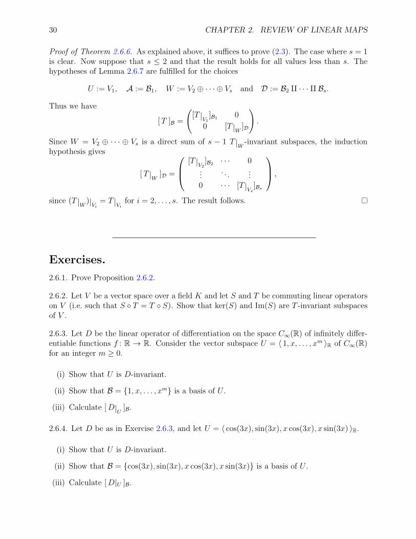
Proof of Theorem 2.6.6. As explained above, it suffices to prove (2.3). The case where s = 1is clear. Now suppose that s ≤ 2 and that the result holds for all values less than s. Thehypotheses of Lemma 2.6.7 are fulfilled for the choices
U := V1, A := B1, W := V2 ⊕ · · · ⊕ Vs and D := B2 q · · · q Bs.
Thus we have
[T ]B =
([T |V1 ]B1 0
0 [T |W ]D
).
Since W = V2 ⊕ · · · ⊕ Vs is a direct sum of s − 1 T |W -invariant subspaces, the inductionhypothesis gives
[T |W ]D =
[T |V2 ]B2 · · · 0...
. . ....
0 · · · [T |Vs ]Bs
,
since (T |W )|Vi = T |Vi for i = 2, . . . , s. The result follows.
Exercises.
2.6.1. Prove Proposition 2.6.2.
2.6.2. Let V be a vector space over a field K and let S and T be commuting linear operatorson V (i.e. such that S ◦ T = T ◦ S). Show that ker(S) and Im(S) are T -invariant subspacesof V .
2.6.3. Let D be the linear operator of differentiation on the space C∞(R) of infinitely differ-entiable functions f : R → R. Consider the vector subspace U = 〈 1, x, . . . , xm 〉R of C∞(R)for an integer m ≥ 0.
(i) Show that U is D-invariant.
(ii) Show that B = {1, x, . . . , xm} is a basis of U .
(iii) Calculate [D|U ]B.
2.6.4. Let D be as in Exercise 2.6.3, and let U = 〈 cos(3x), sin(3x), x cos(3x), x sin(3x) 〉R.
(i) Show that U is D-invariant.
(ii) Show that B = {cos(3x), sin(3x), x cos(3x), x sin(3x)} is a basis of U .
(iii) Calculate [D|U ]B.

2.6. ENDOMORPHISMS AND INVARIANT SUBSPACES 31
2.6.5. Let V be a vector space of dimension 4 over Q, let A = {v1,v2,v3,v4} be a basis ofV , and let T : V → V be the linear map determined by the conditions
T (v1) = v1 + v2 + 2v3, T (v2) = v1 + v2 + 2v4,
T (v3) = v1 − 3v2 + v3 − v4, T (v4) = −3v1 + v2 − v3 + v4.
(i) Show that B1 = {v1 +v2, v3 +v4} and B2 = {v1−v2, v3−v4} are bases (respectively)of T -invariant subspaces V1 and V2 of V such that V = V1 ⊕ V2.
(ii) Calculate [T |V1 ]B1 and [T |V2 ]B2 . Then find [T ]B, where B = B1
∐B2.
2.6.6. Let T : R3 → R3 be the linear map whose matrix relative to the standard basis E ofR3 is
[T ]E =
−1 2 22 −1 22 2 −1
.
(i) Show that B1 = {(1, 1, 1)t} and B2 = {(1,−1, 0)t, (0, 1,−1)t} are bases (respectively)of T -invariant subspaces V1 and V2 of R3 such that R3 = V1 ⊕ V2.
(ii) Calculate [T |V1 ]B1 and [T |V2 ]B2 , and deduce [T ]B, where B = B1
∐B2.
2.6.7. Let V be a finite dimensional vector space over a field K, let T : V → V be an endomor-phism of V , and let n = dimK(V ). Suppose that there exists an integer m ≥ 0 and a vectorv ∈ V such that V = 〈v, T (v), T 2(v), . . . , Tm(v) 〉K . Show that B = {v, T (v), . . . , T n−1(v)}is a basis of V and that there exist a0, . . . , an−1 ∈ K such that
[T ]B =
0 0 . . . 0 a0
1 0 . . . 0 a1
0 1 . . . 0 a2...
.... . .
......
0 0 . . . 1 an−1
.
Note. We say that a vector spacel V with the above property is T -cyclic, or simply cyclic.
The last three exercises give examples of the general situation discussed in Exercise 2.6.7.
2.6.8. Let T : R2 → R2 be the linear map whose matrix in the standard basis E is
[T ]E =
(1 23 1
).
(i) Let v = (1, 1)t. Show that B = {v, T (v)} is a basis of R2.
(ii) Determine [T 2(v)]B.

32 CHAPTER 2. REVIEW OF LINEAR MAPS
(iii) Calculate [T ]B.
2.6.9. Let V be a vector space of dimension 3 over Q, let A = {v1,v2,v3} be a basis of V ,and let T : V → V be the linear map determined by the conditions
T (v1) = v1 + v3, T (v2) = v1 − v2 and T (v3) = v2.
(i) Find [T ]A.
(ii) Show that B = {v1, T (v1), T 2(v1)} is a basis of V .
(iii) Calculate [T ]B.
2.6.10. Let V = 〈 1, ex, e2x 〉R ⊂ C∞(R) and let D be the restriction to V of the operator ofderivation on C∞(R). Then A = {1, ex, e2x} is a basis of V (you do not need to show this).
(i) Let f(x) = 1 + ex + e2x. Show that B = { f, D(f), D2(f) } is a basis of V .
(ii) Calculate [D ]B.

Chapter 3
Review of diagonalization
In this chapter, we recall how to determine if a linear operator or a square matrix is diago-nalizable and, if so, how to diagonalize it.
3.1 Determinants and similar matrices
Let K be a field. We define the determinant of a square matrix A = (aij) ∈ Matn×n(K) by
det(A) =∑
(j1,...,jn)∈Sn
ε(j1, . . . , jn)a1j1 · · · anjn
where Sn denotes the set of permutations of (1, 2, . . . , n) and where, for a permutation(j1, . . . , jn) ∈ Sn, the expression ε(j1, . . . , jn) represents the signature of (j1, . . . , jn), givenby
ε(j1, . . . , jn) = (−1)N(j1,...,jn)
where N(j1, . . . , jn) denotes the number of pairs of indices (k, l) with 1 ≤ k < l ≤ n andjk > jl (called the number of inversions of (j1, . . . , jn)).
Recall that the determinant satisfies the following properties:
Theorem 3.1.1. Let n ∈ N>0 and let A,B ∈ Matn×n(K). Then we have:
(i) det(I) = 1,
(ii) det(At) = det(A),
(iii) det(AB) = det(A) det(B),
where I denotes the n× n identity matrix and At denotes the transpose of A. Moreover, thematrix A is invertible if and only if det(A) 6= 0, in which case
33

34 CHAPTER 3. REVIEW OF DIAGONALIZATION
(iv) det(A−1) = det(A)−1.
In fact, the above formula for the determinant applies to any square matrix with coeffi-cients in a commutative ring. A proof of Theorem 3.1.1 in the general case, with K replacedby an arbitrary commutative ring, can be found in Appendix B.
The “multiplicative” properties (iii) and (iv) of the determinant imply the followingresult.
Proposition 3.1.2. Let T be an endomorphism of a finite dimensional vector space V , andlet B, B′ be two bases of V . Then we have
det[T ]B = det[T ]B′ .
Proof. We have [T ]B′ = P−1[T ]BP where P = [ IV ]B′B , and so
det[T ]B′ = det(P−1[T ]BP )
= det(P−1) det[T ]B det(P )
= det(P )−1 det[T ]B det(P )
= det[T ]B.
This allows us to formulate the following:
Definition 3.1.3 (Determinant). Let T : V → V be a linear operator on a finite dimensionalvector space V . We define the determinant of T by
det(T ) = det[T ]B
where B denotes an arbitrary basis of V .
Theorem 3.1.1 allows us to study the behavior of the determinant under the compositionof linear operators:
Theorem 3.1.4. Let S and T be linear operators on a finite dimensional vector space V .We have:
(i) det(IV ) = 1,
(ii) det(S ◦ T ) = det(S) det(T ).
Moreover, T is invertible if and only if det(T ) 6= 0, in which case we have
(iii) det(T−1) = det(T )−1.

3.1. DETERMINANTS AND SIMILAR MATRICES 35
Proof. Let B be a basis of V . Since [ IV ]B = I is the n × n identity matrix, we havedet(IV ) = det(I) = 1. This proves (i). For (iii), we note, by Corollary 2.4.7, that T isinvertible if and only if the matrix [T ]B is invertible and that, in this case,
[T−1]B = [T ]−1B .
This proves (iii). Relation (ii) is left as an exercise.
Theorem 3.1.4 illustrates the phenomenon mentioned in the introduction that, most ofthe time in this course, a result about matrices implies a corresponding result about linearoperators and vice-versa. We conclude with the following notion:
Definition 3.1.5 (Similarity). Let n ∈ N>0 and let A,B ∈ Matn×n(K) be square matrices ofthe same size n × n. We say that A is similar to B (or conjugate to B), if there exists aninvertible matrix P ∈ Matn×n(K), such that B = P−1AP . We then write A ∼ B.
Example 3.1.6. If T : V → V is a linear operator on a finite dimensional vector space V andif B and B′ are two bases of V , then we have
[T ]B′ = P−1 [T ]BP
where P = [ IV ]B′B , and so [T ]B′ and [T ]B are similar.
More precisely, we can show:
Proposition 3.1.7. Let T : V → V be a linear operator on a finite dimensional vector spaceV , and let B be a basis of V . A matrix M is similar to [T ]B if and only if there exists abasis B′ of V such that M = [T ]B′.
Finally, Theorem 3.1.1 provides a necessary condition for two matrices to be similar:
Proposition 3.1.8. If A and B are two similar matrices, then det(A) = det(B).
The proof is left as an exercise. Proposition 3.1.2 can be viewed as a corollary to thisresult, together with Example 3.1.6.
Exercises.
3.1.1. Show that similarity ∼ is an equivalence relation on Matn×n(K).
3.1.2. Prove Proposition 3.1.7.
3.1.3. Prove Proposition 3.1.8.

36 CHAPTER 3. REVIEW OF DIAGONALIZATION
3.2 Diagonalization of operators
In this section, we fix a vector space V of finite dimension n over a field K and a linearoperator T : V → V . We say that:
• T is diagonalizable if there exists a basis B of V such that [T ]B is a diagonal matrix,
• an element λ of K is an eigenvalue of T if there exists a nonzero vector v of V suchthat
T (v) = λv ,
• a nonzero vector v that satisfies the above relation for an element λ of K is called aneigenvector of T or, more precisely, an eigenvector of T for the eigenvalue λ.
We also recall that if λ ∈ K is an eigenvalue of T then the set
Eλ := {v ∈ V ; T (v) = λv}
(also denoted Eλ(T )) is a subspace of V since, for v ∈ V , we have
T (v) = λv ⇐⇒ (T − λI)(v) = 0
and soEλ = ker(T − λI).
We way that Eλ is the eigenspace of T for the eigenvalue λ. The eigenvectors of T for thiseigenvalue are the nonzero elements of Eλ.
For each eigenvalue λ ∈ K, the eigenspace Eλ is a T -invariant subspace of V since, ifv ∈ Eλ, we have T (v) = λv ∈ Eλ. Also note that an element v of V is an eigenvector of Tif and only if 〈v〉K is a T -invariant subspace of V of dimension 1 (exercise).
Proposition 3.2.1. The operator T is diagonalizable if and only if V admits a basis con-sisting of eigenvectors of T .
Proof. Let B = {v1, . . . ,vn} be a basis of V , and let λ1, . . . , λn ∈ K. We have
[T ]B =
λ1 0. . .
0 λn
⇐⇒ T (v1) = λ1v1 , . . . , T (vn) = λnvn.
The conclusion follows.

3.2. DIAGONALIZATION OF OPERATORS 37
The crucial point is the following result:
Proposition 3.2.2. Let λ1, . . . , λs ∈ K be distinct eigenvalues of T . The sum Eλ1 +· · ·+Eλsis direct.
Proof. In light of Definition 1.4.1, we need to show that the only possible choice of vectorsv1 ∈ Eλ1 , . . . ,vs ∈ Eλs such that
v1 + · · ·+ vs = 0 (3.1)
is v1 = · · · = vs = 0. We show this by induction on s, noting first that, for s = 1, the resultis immediate.
Suppose that s ≥ 2 and that the sum Eλ1 + · · · + Eλs−1 is direct. Choose vectorsv1 ∈ Eλ1 , . . . ,vs ∈ Eλs satisfying (3.1) and apply T to both sides of this equality. SinceT (vi) = λivi for i = 1, . . . , s and T (0) = 0, we get
λ1v1 + · · ·+ λsvs = 0. (3.2)
Subtracting from (3.2) the equality (3.1) multiplied by λs, we have
(λ1 − λs)v1 + · · ·+ (λs−1 − λs)vs−1 = 0.
Since (λi − λs)vi ∈ Eλi for i = 1, . . . , s− 1 and, by hypothesis, the sum Eλ1 + · · ·+Eλs−1 isdirect, we see that
(λ1 − λs)v1 = · · · = (λs−1 − λs)vs−1 = 0.
Finally, since λs 6= λi for i = 1, . . . , s − 1, we conclude that v1 = · · · = vs−1 = 0, hence,by (3.1), that vs = 0. Therefore the sum Eλ1 + · · ·+ Eλs is direct.
From this we conclude the following:
Theorem 3.2.3. The operator T has at most n = dimK(V ) eigenvalues. Let λ1, . . . , λs bethe distinct eigenvalues of T in K. Then T is diagonalizable if and only if
dimK(V ) = dimK(Eλ1) + · · ·+ dimK(Eλs).
If this is the case, we obtain a basis B of V consisting of eigenvectors of T by concatenatingbases of Eλ1 , . . . , Eλs and
[T ]B =
λ1
. . .
λ1
0. . .
0λs
. . .
λs
with each λi repeated a number of times equal to dimK(Eλi).
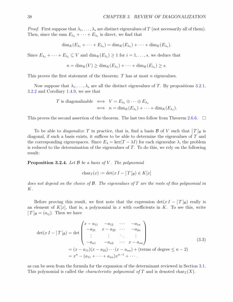
38 CHAPTER 3. REVIEW OF DIAGONALIZATION
Proof. First suppose that λ1, . . . , λs are distinct eigenvalues of T (not necessarily all of them).Then, since the sum Eλ1 + · · ·+ Eλs is direct, we find that
dimK(Eλ1 + · · ·+ Eλs) = dimK(Eλ1) + · · ·+ dimK(Eλs).
Since Eλ1 + · · ·+ Eλs ⊆ V and dimK(Eλi) ≥ 1 for i = 1, . . . , s, we deduce that
n = dimK(V ) ≥ dimK(Eλ1) + · · ·+ dimK(Eλs) ≥ s.
This proves the first statement of the theorem: T has at most n eigenvalues.
Now suppose that λ1, . . . , λs are all the distinct eigenvalues of T . By propositions 3.2.1,3.2.2 and Corollary 1.4.9, we see that
T is diagonalizable ⇐⇒ V = Eλ1 ⊕ · · · ⊕ Eλs⇐⇒ n = dimK(Eλ1) + · · ·+ dimK(Eλs).
This proves the second assertion of the theorem. The last two follow from Theorem 2.6.6.
To be able to diagonalize T in practice, that is, find a basis B of V such that [T ]B isdiagonal, if such a basis exists, it suffices to be able to determine the eigenvalues of T andthe corresponding eigenvspaces. Since Eλ = ker(T − λI) for each eigenvalue λ, the problemis reduced to the determination of the eigenvalues of T . To do this, we rely on the followingresult:
Proposition 3.2.4. Let B be a basis of V . The polynomial
charT (x) := det(x I − [T ]B) ∈ K[x]
does not depend on the choice of B. The eigenvalues of T are the roots of this polynomial inK.
Before proving this result, we first note that the expression det(x I − [T ]B) really isan element of K[x], that is, a polynomial in x with coefficients in K. To see this, write[T ]B = (aij). Then we have
det(x I − [T ]B) = det
x− a11 −a12 · · · −a1n
−a21 x− a22 · · · −a2n...
.... . .
...−an1 −an2 · · · x− ann
= (x− a11)(x− a22) · · · (x− ann) + (terms of degree ≤ n− 2)
= xn − (a11 + · · ·+ ann)xn−1 + · · · .
(3.3)
as can be seen from the formula for the expansion of the determinant reviewed in Section 3.1.This polynomial is called the characteristic polynomial of T and is denoted charT (X).

3.2. DIAGONALIZATION OF OPERATORS 39
Proof of Proposition 3.2.4. Let B′ be another basis of V . We know that
[T ]B′ = P−1[T ]B P
where P = [ I ]B′B . We thus have
xI − [T ]B′ = xI − P−1[T ]B P = P−1(xI − [T ]B)P,
and sodet(xI − [T ]B′) = det
(P−1(xI − [T ]B)P
)= det(P )−1 det(xI − [T ]B) det(P )
= det(xI − [T ]B).
(3.4)
This shows that the polynomial det(xI − [T ]B) is independent of the choice of B. Note thatthe calculations (3.4) involve matrices with polynomial coefficients in K[x], and the multi-plicativity of the determinant for a product of such matrices. This is justified in AppendixB. If the field K if infinite, we can avoid this difficulty by identifying the polynomials inK[x] with polynomial functions from K to K (see Section 4.2).
Finally, let λ ∈ K. Be definition, λ is an eigenvalue of T if and only if
ker(T − λI) 6= {0} ⇐⇒ there exists v ∈ V \ {0} such that (T − λ I)v = 0 ,
⇐⇒ there exists X ∈ Kn \ {0} such that [T − λ I ]BX = 0 ,
⇐⇒ det([T − λ I ]B) = 0 .
Since [T − λI ]B = [T ]B − λ[ I ]B = [T ]B − λI = −(λI − [T ]B), we also have
det([T − λI ]B) = (−1)ncharT (λ) .
Thus the eigenvalues of T are the roots of charT (x).
Corollary 3.2.5. Let B be a basis of V . Writes [T ]B = (aij). Then the number
trace(T ) := a11 + a22 + · · ·+ ann,
called the trace of T , does not depend on the choice of B. We have
charT (x) = xn − trace(T )xn−1 + · · ·+ (−1)n det(T ).
Proof. The calculations (3.3) show that the coefficient of xn−1 in det(x I − [T ]B) is equalto −(a11 + · · · + ann). Since charT (x) = det(xI − [T ]B) does not depend on the choice ofB, the sum a11 + · · · + ann does not depend on it either. This proves the first assertionof the corollary. For the second, it suffices to show that the constant term of charT (x) is(−1)n det(T ). But this coefficient is
charT (0) = det(−[T ]B) = (−1)n det([T ]B) = (−1)n det(T ).

40 CHAPTER 3. REVIEW OF DIAGONALIZATION
Example 3.2.6. With the notation of Example 2.6.5, we set T = D|U where U is the subspace
of C∞(R) generated by the functions f1(x) = e2x, f2(x) = x e2x and f3(x) = x2e2x, and whereD is the derivative operator on C∞(R). We have seen that B = {f1, f2, f3} is a basis for Uand that
[T ]B =
2 1 00 2 20 0 2
.
The characteristic polynomial of T is therefore
charT (x) = det(xI − [T ]B) =
∣∣∣∣∣∣x− 2 −1 0
0 x− 2 −20 0 x− 2
∣∣∣∣∣∣ = (x− 2)3.
Since x = 2 is the only root of (x− 2)3 in R, we see that 2 is the only eigenvalue of T . Theeigenspace of T for this eigenvalue is
E2 = ker(T − 2I).
Let f ∈ U . We have
f ∈ E2 ⇐⇒ (T − 2I)(f) = 0 ⇐⇒ [T − 2I ]B[f ]B = 0 ⇐⇒ ([T ]B − 2I)[f ]B = 0
⇐⇒
0 1 00 0 20 0 0
[f ]B = 0 ⇐⇒ [f ]B =
t00
with t ∈ R
⇐⇒ f = t f1 with t ∈ R .
Thus E2 = 〈f1〉R has dimension 1. Since
dimR(E2) = 1 6= 3 = dimR(U),
Theorem 3.2.3 tells us that T is not diagonalizable.
Exercises.
3.2.1. Let V be a vector space over a field K, let T : V → V be a linear operator on V , andlet v1, . . . ,vs be eigenvectors of T for the distinct eigenvalues λ1, . . . , λs ∈ K. Show thatv1, . . . ,vs are linearly independent over K.
Hint. You can, for example, combine Proposition 3.2.2 with Exercise 1.4.3(ii).
3.2.2. Let V = 〈 f0, f1, . . . , fn 〉R be the subspace of C∞(R) generated by the functions fi(x) =eix for i = 0, . . . , n.

3.3. DIAGONALIZATION OF MATRICES 41
(i) Show that V is invariant under the operator D of derivation on C∞(R) and that, fori = 0, . . . , n, the function fi is an eigenvector of D with eigenvalue i.
(ii) Using Exercise 3.2.1, deduce that B = {f0, f1, . . . , fn} is a basis of V .
(iii) Calculate [D|V ]B.
3.2.3. Consider the subspace P2(R) of C∞(R) given by P2(R) = 〈 1, x, x2 〉R. In each case,determine whether or not the given linear map is diagonalizable and, if it is, find a basiswith respect to which its matrix is diagonal.
(i) T : P2(R)→ P2(R) given by T (p(x)) = p′(x).
(ii) T : P2(R)→ P2(R) given by T (p(x)) = p(2x).
3.2.4. Let T : Mat2×2(R)→ Mat2×2(R) be the linear map given by T (A) = At.
(i) Find a basis of the eigenspaces of T for the eigenvalues 1 and −1.
(ii) Find a basis B of Mat2×2(R) such that [T ]B is diagonal, and write [T ]B.
3.2.5. Let S : R3 → R3 be the reflection in the plane with equation x+ y + z = 0.
(i) Describe geometrically the eigenspaces of S and give a basis of each.
(ii) Find a basis B of R3 relative to which the matrix of S is diagonal and give [S ]B.
(iii) Using the above, find the matrix of T in the standard basis.
3.3 Diagonalization of matrices
As we have already mentioned, results on linear operators translate into results on matricesand vice versa. The problem of diagonalization is a good example of this.
In this section, we fix an integer n ≥ 1.
• We say that a matrix A ∈ Matn×n(K) is diagonalizable if there exists an invertiblematrix P ∈ Matn×n(K) such that P−1AP is a diagonal matrix.
• We say that an element λ of K is an eigenvalue of A if there exists a nonzero columnvector X ∈ Kn such that AX = λX.

42 CHAPTER 3. REVIEW OF DIAGONALIZATION
• A nonzero column vector X ∈ Kn that satisfies the relation AX = λX for a scalarλ ∈ K is called an eigenvector of A for the eigenvalue λ.
• If λ is an eigenvalue of A, then the set
Eλ(A) := {X ∈ Kn ; AX = λX}= {X ∈ Kn ; (A− λI)X = 0}
is a subspace of Kn called the eigenspace of A for the eigenvalue λ.
• The polynomial
charA(x) := det(x I − A) ∈ K[x]
is called the characteristic polynomial of A.
Recall that to every A ∈ Matn×n(K), we associate a linear operator TA : Kn → Kn givenby
TA(X) = AX for all X ∈ Kn.
Then we see that the above definitions coincide with the corresponding notions for theoperator TA. More precisely, we note that:
Proposition 3.3.1. Let A ∈ Matn×n(K).
(i) The eigenvalues of TA coincide with those of A.
(ii) If λ is an eigenvalue TA, then the eigenvectors of TA for this eigenvalue are the sameas those of A and we have Eλ(TA) = Eλ(A).
(iii) charTA(x) = charA(x).
Proof. Assertions (i) and (ii) follow directly from the definitions, while (iii) follows from thefact that [TA ]E = A, where E is the standard basis of Kn.
We also note that:
Proposition 3.3.2. Let A ∈ Matn×n(K). The following conditions are equvalent:
(i) TA is diagonalizable,
(ii) there exists a basis of Kn consisting of eigenvectors of A,
(iii) A is diagonalizable.

3.3. DIAGONALIZATION OF MATRICES 43
Furthermore, if these conditions are satisfied and if B = {X1, . . . , Xn} is a basis of Kn
consisting of eigenvectors of A, then the matrix P = (X1 · · ·Xn) is invertible and
P−1AP =
λ1 0. . .
0 λn
,
where λi is the eigenvalue of A corresponding to Xi for i = 1, . . . , n.
Proof. If TA is diagonalizable, Proposition 3.2.1 shows that there exists a basis B = {X1, . . . , Xn}of Kn consisting of eigenvectors of TA or, equivalently, of A. For such a basis, the change ofbasis matrix P = [ I ]BE = (X1 · · ·Xn) from the basis B to the standard basis E is invertibleand we find that
P−1AP = P−1[TA ]EP = [TA ]B =
λ1 0. . .
0 λn
,
where λi is the eigenvalue of A corresponding to Xi for i = 1, . . . , n. This proves theimplication (i)⇒(ii)⇒(iii) as well as the last assertion of the proposition. It remains toprove the implication (iii)⇒(i).
Suppose therefore that A is diagonalizable and that P ∈ Matn×n(K) is an invertiblematrix such that P−1AP is diagonal. Since P is invertible, its columns form a basis B ofKn and, with this choice of basis, we have P = [ I ]BE . Then [TA ]B = P−1[TA ]EP = P−1APis diagonal, which proves that TA is diagonalizable.
Combining Theorem 3.2.3 with the two preceding propositions, we have the following:
Theorem 3.3.3. Let A ∈ Matn×n(K). Then A has an most n eigenvalues in K. Letλ1, . . . , λs be the distinct eigenvalues of A in K. Then A is diagonalizable if and only if
n = dimK(Eλ1(A)) + · · ·+ dimK(Eλs(A)) .
If this is the case, we obtain a basis B = {X1, . . . , Xn} of Kn consisting of eigenvectors ofA by concatenating the bases Eλ1(A), . . . , Eλs(A). Then the matrix P = (X1 · · ·Xn) withcolumns X1, . . . , Xn is invertible and
P−1AP =
λ1
. . .
λ1
0. . .
0λs
. . .
λs
with each λi repeated a number of times equal to dimK(Eλi(A)).
44 CHAPTER 3. REVIEW OF DIAGONALIZATION
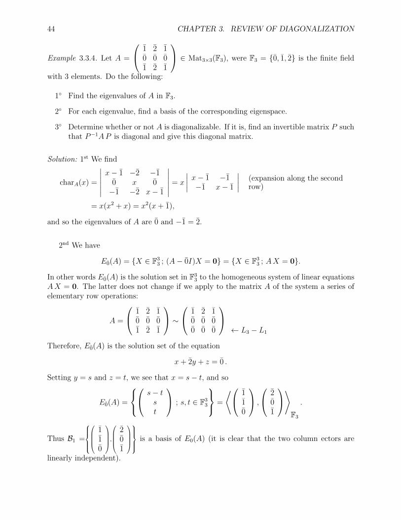
Example 3.3.4. Let A =
1 2 10 0 01 2 1
∈ Mat3×3(F3), were F3 = {0, 1, 2} is the finite field
with 3 elements. Do the following:
1◦ Find the eigenvalues of A in F3.
2◦ For each eigenvalue, find a basis of the corresponding eigenspace.
3◦ Determine whether or not A is diagonalizable. If it is, find an invertible matrix P suchthat P−1AP is diagonal and give this diagonal matrix.
Solution: 1st We find
charA(x) =
∣∣∣∣∣∣x− 1 −2 −1
0 x 0−1 −2 x− 1
∣∣∣∣∣∣ = x
∣∣∣∣ x− 1 −1−1 x− 1
∣∣∣∣ (expansion along the secondrow)
= x(x2 + x) = x2(x+ 1),
and so the eigenvalues of A are 0 and −1 = 2.
2nd We have
E0(A) = {X ∈ F33 ; (A− 0I)X = 0} = {X ∈ F3
3 ; AX = 0}.
In other words E0(A) is the solution set in F33 to the homogeneous system of linear equations
AX = 0. The latter does not change if we apply to the matrix A of the system a series ofelementary row operations:
A =
1 2 10 0 01 2 1
∼ 1 2 1
0 0 00 0 0
← L3 − L1
Therefore, E0(A) is the solution set of the equation
x+ 2y + z = 0 .
Setting y = s and z = t, we see that x = s− t, and so
E0(A) =
s− t
st
; s, t ∈ F33
=
⟨ 110
,
201
⟩F3
.
Thus B1 =
110
,
201
is a basis of E0(A) (it is clear that the two column ectors are
linearly independent).

3.3. DIAGONALIZATION OF MATRICES 45
Similarly, we have:
E2(A) = {X ∈ F33 ; (A− 2I)X = 0} = {X ∈ F3
3 ; (A+ I)X = 0} .
We find
A+ I =
2 2 10 1 01 2 2
∼ 1 1 2
0 1 01 2 2
← 2L1
∼
1 1 20 1 00 1 0
← L3−L1
∼
1 0 20 1 00 0 0
← L1−L2
← L3−L2
Therefore, E2(A) is the solution set to the system{x + 2z = 0
y = 0.
Here, z is the only independent variable. Let z = t. Then x = −2t = t and y = 0, and so
E2(A) =
t
0t
; t ∈ F3
=
⟨ 101
⟩F3
and it follows that B2 =
101
is a basis of E2(A).
3rd Since A is a 3× 3 matrix and
dimF3 E0(A) + dimF3 E2(A) = 3,
we conclude that A is diagonalizable, and that
B = B1 q B2 =
1
10
,
201
,
101
is a basis of F3
3 consisting of eigenvectors of A for the respective eigenvalues 0, 0, 2. Then thematrix
P =
1 2 11 0 00 1 1
is invertible and the product P−1AP is a diagonal matrix with diagonal (0, 0, 2):
P−1AP =
0 0 00 0 00 0 2
.

46 CHAPTER 3. REVIEW OF DIAGONALIZATION
Exercises.
3.3.1. In each case, find the real eigenvalues of the given matrix A ∈ Mat3×3(R) and, foreach of the eigenvalues, give a basis of the corresponding eigenspace. If A is diagonalizable,find an invertible matrix P ∈ Mat3×3(R) such that P−1AP is diagonal, and give P−1AP .
(i) A =
−2 0 50 5 0−4 0 7
, (ii) A =
1 −2 32 6 −61 2 −1
.
3.3.2. The matrix A =
(1 −24 −3
)is not diagonalizable over the real numbers. However, it
is over the complex numbers. Find an invertible matrix P with complex entries such thatP−1AP is diagonal, and give P−1AP .
3.3.3. Let F2 = {0, 1} be the field with 2 elements and let A =
1 1 11 0 00 0 1
∈ Mat3×3(F2).
Find the eigenvalues of A in F2 and, for each one, give a basis of the corresponding eigenspace.If A is diagonalizable, find an invertible matrix P ∈ Mat3×3(F2) such that P−1AP is diagonal,and give P−1AP .

Chapter 4
Polynomials, linear operators andmatrices
Let V be a vector space of finite dimension n over a field K. In this chapter, we show that theset EndK(V ) of linear operators on V is a ring under addition and composition, isomorphicto the ring Matn×n(K) of n × n matrices with coefficients in K. We then construct thering K[x] of polynomials in one indeterminate x over the field K. For each linear operatorT ∈ EndK(V ) and each matrix A ∈ Matn×n(K), we define ring homomorphisms
K[x] −→ EndK(V ) and K[x] −→ Matn×n(K)P (x) 7−→ P (T ) P (x) 7−→ P (A)
that send x to T and x to A respectively. The link between them is that, if B is a basis ofV , then [P (T )]B = P ([T ]B).
4.1 The ring of linear operators
We refer the reader to Appendix A for a review of the basic notions related to rings. Wefirst show:
Theorem 4.1.1. Let V be a vector space of dimension n over a field K and let B be a basisof V . The set EndK(V ) of linear operators on V is a ring under addition and composition.Furthermore, the function
ϕ : EndK(V ) −→ Matn×n(K)T 7−→ [T ]B
is a ring isomorphism.
Proof. We already know, by Theorem 2.2.3, that the set EndK(V ) = LK(V, V ) is a vectorspace over K. In particular, it is an abelian group under addition. We also know that the
47

48 CHAPTER 4. POLYNOMIALS, LINEAR OPERATORS AND MATRICES
composite of two linear operators S : V → V and T : V → V is a linear operator S ◦T : V →V , hence an element of EndK(V ). Since the composition is associative and the identity mapIV ∈ EndK(V ) is an identity element for this operation, we conclude that EndK(V ) is amonoid under composition. Finally, Proposition 2.3.1 gives that if R, S, T ∈ EndK(V ), then
(R + S) ◦ T = R ◦ T + S ◦ T and R ◦ (S + T ) = R ◦ S +R ◦ T.
Therefore composition is distributive over addition in EndK(V ) and so EndK(V ) is a ring.
In addition, Theorem 2.4.3 shows that the function ϕ is an isomorphism of vector spacesover K. In particular, it is an isomorphism of abelian groups under addition. Finally,Proposition 2.4.6 implies that if S, T ∈ EndK(V ), then
ϕ(S ◦ T ) = [S ◦ T ]B = [S ]B[T ]B = ϕ(S)ϕ(T ) .
Since ϕ(IV ) = I, we conclude that ϕ is also an isomorphism of rings.
Exercises.
4.1.1. Let V be a vector space over a field K and let U be a subspace of V . Show that theset of linear maps T : V → V such that T (u) ∈ U for all u ∈ U is a subring of EndK(V ).
4.1.2. Let A = {a+ b√
2 ; a, b ∈ Q}.
(i) Show that A is a subring of R and that B = {1,√
2} is a basis of A viewed as a vectorspace over Q.
(ii) Let α = a+ b√
2 ∈ A. Show that the function mα : A→ A defined by mα(β) = αβ forall β ∈ A is a Q-linear map and calculate [mα]B.
(iii) Show that the function ϕ : A→ Mat2×2(Q) given by ϕ(α) = [mα]B is an injective ringhomomorphism, and describe its image.
4.2 Polynomial rings
Proposition 4.2.1. Let A be a commutative ring and let x be a symbol not in A. Thereexists a commutative ring, denoted A[x], containing A as a subring and x as an element suchthat
(i) every element of A[x] can be written as a0 + a1 x+ · · ·+ an xn for some integer n ≥ 0
and some elements a0, a1, . . . , an of A ;
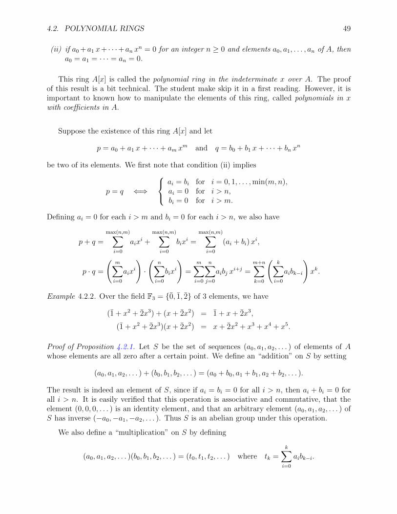
4.2. POLYNOMIAL RINGS 49
(ii) if a0 +a1 x+ · · ·+an xn = 0 for an integer n ≥ 0 and elements a0, a1, . . . , an of A, then
a0 = a1 = · · · = an = 0.
This ring A[x] is called the polynomial ring in the indeterminate x over A. The proofof this result is a bit technical. The student make skip it in a first reading. However, it isimportant to known how to manipulate the elements of this ring, called polynomials in xwith coefficients in A.
Suppose the existence of this ring A[x] and let
p = a0 + a1 x+ · · ·+ am xm and q = b0 + b1 x+ · · ·+ bn x
n
be two of its elements. We first note that condition (ii) implies
p = q ⇐⇒
ai = bi for i = 0, 1, . . . ,min(m,n),ai = 0 for i > n,bi = 0 for i > m.
Defining ai = 0 for each i > m and bi = 0 for each i > n, we also have
p+ q =
max(n,m)∑i=0
aixi +
max(n,m)∑i=0
bixi =
max(n,m)∑i=0
(ai + bi)xi,
p · q =
(m∑i=0
aixi
)·
(n∑i=0
bixi
)=
m∑i=0
n∑j=0
aibj xi+j =
m+n∑k=0
(k∑i=0
aibk−i
)xk.
Example 4.2.2. Over the field F3 = {0, 1, 2} of 3 elements, we have
(1 + x2 + 2x3) + (x+ 2x2) = 1 + x+ 2x3,
(1 + x2 + 2x3)(x+ 2x2) = x+ 2x2 + x3 + x4 + x5.
Proof of Proposition 4.2.1. Let S be the set of sequences (a0, a1, a2, . . . ) of elements of Awhose elements are all zero after a certain point. We define an “addition” on S by setting
(a0, a1, a2, . . . ) + (b0, b1, b2, . . . ) = (a0 + b0, a1 + b1, a2 + b2, . . . ).
The result is indeed an element of S, since if ai = bi = 0 for all i > n, then ai + bi = 0 forall i > n. It is easily verified that this operation is associative and commutative, that theelement (0, 0, 0, . . . ) is an identity element, and that an arbitrary element (a0, a1, a2, . . . ) ofS has inverse (−a0,−a1,−a2, . . . ). Thus S is an abelian group under this operation.
We also define a “multiplication” on S by defining
(a0, a1, a2, . . . )(b0, b1, b2, . . . ) = (t0, t1, t2, . . . ) where tk =k∑i=0
aibk−i.

50 CHAPTER 4. POLYNOMIALS, LINEAR OPERATORS AND MATRICES
The result is an element of S, since if we suppose again that ai = bi = 0 for all i > n, then,for every integer k > 2n, each of the products aibk−i with i = 0, . . . , k is zero (one of theindices i or k − i being necessarily > n) and so tk = 0. It is easy to see that the sequence(1, 0, 0, . . . ) is an identity element for this operation.
To conclude that S is a ring under these operations, it remains to show that the mul-tiplication is associative and distributive over the addition. In other words, we must showthat if
p = (a0, a1, a2, . . . ), q = (b0, b1, b2, . . . ) and r = (c0, c1, c2, . . . )
are three elements of S, then
1) (pq)r = p(qr),
2) (p+ q)r = p r + q r,
3) p(q + r) = p q + p r.
These three equalities are proved in the same manner: it suffices to show that the sequenceson either side of the equality have the same element of index k for each k ≥ 0. Equality 1) isthe most delicate to verify since each term involves two products. We see that the elementof index k of (pq)r is
((pq)r)k =k∑j=0
(pq)jck−j =k∑j=0
(j∑i=0
aibj−i
)ck−j =
k∑j=0
j∑i=0
aibj−ick−j
and that of p(qr) is
(p(qr))k =k∑i=0
ai(qr)k−i =k∑i=0
ai
(k−i∑j=0
bjck−i−j
)=
k∑i=0
k−i∑j=0
aibjck−i−j.
In both cases, we see that the result if the sum of all products aibjcl with i, j, l ≥ 0 andi+ j + l = k, hence
((pq)r)k =∑
i+j+l=k
aibjcl = (p(qr))k.
This proves 1). The proofs of 2) and 3) are simpler and left as exercises.
For all a, b ∈ A, we see that
(a, 0, 0, . . . ) + (b, 0, 0, . . . ) = (a+ b, 0, 0, . . . ),
(a, 0, 0, . . . )(b, 0, 0, . . . ) = (ab, 0, 0, . . . ).
Thus the map ι : A→ S given by
ι(a) = (a, 0, 0, . . . )

4.2. POLYNOMIAL RINGS 51
is an injective ring homomorphism. From now on, we identify A with its image under ι.Then A becomes a subring of S and we have
a(b0, b1, . . . ) = (a b0, a b1, a b2, . . . )
for all a ∈ A and every sequence (b0, b1, b2, . . . ) ∈ S.
Let X = (0, 1, 0, 0, . . . ). An easy induction shows that, for every integer i ≥ 1, the i-thpower X i of X is the sequence whose elements are all zero except for the element of index i,which is equal to 1:
X i = (0, . . . , 0,
i∨1, 0, . . . ).
From this we deduce:
1st For every sequence (a0, a1, a2, . . . ) of S, by choosing an integer n ≥ 0 such that ai = 0for all i > n, we have:
(a0, a1, a2, . . . ) =n∑i=0
(0, . . . , 0,
i∨ai, 0, . . . ) =
n∑i=0
ai (0, . . . , 0,
i∨1, 0, . . . ) =
n∑i=0
aiXi.
2nd In addition, if n is an integer ≥ 0 and a0, a1, . . . , an ∈ A satisfy
a0 + a1X + · · ·+ anXn = 0,
then
0 =n∑i=0
ai (0, . . . , 0,
i∨1, 0, . . . ) =
n∑i=0
(0, . . . , 0,
i∨ai, 0, . . . ) = (a0, a1, . . . , an, 0, 0, . . . ),
and so a0 = a1 = · · · = an = 0.
These last two observations show that the ring S has the two properties required by theproposition except that instead of the element x, we have the sequence X = (0, 1, 0, . . . ).This is not really a problem: it suffices to replace X by x in S and in the addition andmultiplication tables of S.
Every polynomial p ∈ A[x] induces a function from A to A. Before giving this construc-tion, we first note the following fact whose proof is left as an exercise:
Proposition 4.2.3. Let X be a set and let A be a commutative ring. The set F(X,A) offunctions from X to A is a commutative ring under the addition and multiplication definedin the following manner. If f, g ∈ F(X,A) then f + g and f g are functions from X to Agiven by
(f + g)(x) = f(x) + g(x) and (f g)(x) = f(x) g(x)
for all x ∈ X.

52 CHAPTER 4. POLYNOMIALS, LINEAR OPERATORS AND MATRICES
We also show:
Proposition 4.2.4. Let A be a subring of a commutative ring C and let c ∈ C. The function
A[x] −→ Cn∑i=0
aixi 7−→
n∑i=0
aici (4.1)
is a ring homomorphism.
This homomorphism is called evaluation at c and the image of a polynomial p under thishomomorphism is denoted p(c).
Proof of Proposition 4.2.4. Let
p =n∑i=0
aixi and q =
m∑i=0
bixi
be elements of A[x]. Define ai = 0 for all i > n and bi = 0 for all i > m. Then we have:
p+ q =
max(n,m)∑i=0
(ai + bi)xi and p q =
m+n∑k=0
(k∑i=0
aibk−i
)xk.
We see that
p(c) + q(c) =m∑i=0
aici +
n∑i=0
bici =
max(n,m)∑i=0
(ai + bi) ci = (p+ q)(c)
and
p(c)q(c) =
(m∑i=0
aici
)(n∑i=0
bici
)=
m∑i=0
n∑j=0
aibj ci+j =
m+n∑k=0
(k∑i=0
aibk−i
)ck = (pq)(c).
These last equalities, together with the fact that the image of 1 ∈ A[x] is 1 show that thefunction (4.1) is indeed a ring homomorphism.
In particular, if we take C = A[x] and c = x, the map 4.1 becomes the identity map:
A[x] −→ A[x]
p =n∑i=0
aixi 7−→ p(x) =
n∑i=0
aixi.
For this reason, we generally write p(x) to denote a polynomial in A[x]. This is what we willgenerally do from now on.

4.2. POLYNOMIAL RINGS 53
Proposition 4.2.5. Let A be a commutative ring. For each p ∈ A[x], denote by Φ(p) : A→A the function given by Φ(p)(a) = p(a) for all a ∈ A. The map Φ : A[x] → F(A,A) thusdefined is a ring homomorphism with kernel
ker(Φ) = {p ∈ A[x] ; p(a) = 0 for all a ∈ A}.
We say that Φ(p) is the polynomial function from A to A induced by p. The image of Φin F(A,A) is called the ring of polynomial functions from A to A. More concisely, we candefine Φ in the following manner:
Φ : A[x] −→ F(A,A)
p 7−→ Φ(p) : A −→ Aa 7−→ p(a)
Proof. Let p, q ∈ A[x]. For all a ∈ A, we have
Φ(p+ q)(a) = (p+ q)(a) = p(a) + q(a) = Φ(p)(a) + Φ(q)(a),
Φ(p q)(a) = (p q)(a) = p(a) q(a) = Φ(p)(a) · Φ(q)(a),
hence Φ(p + q) = Φ(p) + Φ(q) and Φ(p q) = Φ(p)Φ(q). Since Φ(1) is the constant functionequal to 1 (the identity element of F(A,A) for the product), we conclude that Φ is a ringhomomorphism. The last assertion concerning its kernel follows from the definitions.
Example 4.2.6. If A = R, the function Φ: R[x] → F(R,R) defined by Proposition 4.2.5is injective, since we know that a nonzero polynomial in R[x] has a finite number of realroots and thus ker Φ = {0}. In this case, Φ induces an isomorphism between the ring R[x] ofpolynomials with coefficients in R and its image in F(R,R), the ring of polynomials functionsfrom R to R.
Example 4.2.7. Let A = F2 = {0, 1}, the field with two elements. The ring F(F2,F2) offunctions from F2 to itself consists of 4 elements whereas F2[x] contains an infinite numberof polynomials. In this case, the map Φ is not injective. For example, the polynomialp(x) = x2 − x satisfies p(0) = 0 and p(1) = 0, hence p(x) ∈ ker Φ.
Exercises.
4.2.1. Prove Proposition 4.2.3.
4.2.2. Show that the map Φ: A[x] → F(A,A) of Proposition 4.2.5 is not injective if A is afinite ring.

54 CHAPTER 4. POLYNOMIALS, LINEAR OPERATORS AND MATRICES
4.3 Evaluation at a linear operator or matrix
Let V be a vector space over a field K and let T : V → V be a linear operator on V . Forevery polynomial
p(x) = a0 + a1x+ · · ·+ anxn ∈ K[x],
we setP (T ) = a0I + a1T + · · ·+ anT
n ∈ EndK(V ),
where I denotes the identity map on V .
Proposition 4.3.1. With the above notation, the map
K[x] −→ EndK(V )p(x) 7−→ p(T )
is a ring homomorphism. Its image, denoted K[T ], is the commutative subring of EndK(V )given by
K[T ] = {a0I + a1T + · · ·+ anTn ; n ∈ N>0, a0, . . . , an ∈ K}.
This homomorphism is called evaluation at T .
Proof. By definition, the image of the constant polynomial 1 is the identity element I ofEndK(V ). To conclude that evaluation at T is a ring homomorphism, it remains to showthat if p, q ∈ K[x] are arbitrary polynomials, then
(p+ q)(T ) = p(T ) + q(T ) and (pq)(T ) = p(T ) ◦ q(T ).
The proof for the sum is left as an exercise. The proof for the product uses the fact that,for all a ∈ K and all S ∈ EndK(V ), we have
(a I) ◦ S = S ◦ (a I) = aS.
Write
p =n∑i=0
ai xi and q =
m∑j=0
bj xj.
We see that
p(T ) ◦ q(T ) =(a0I +
n∑i=1
ai Ti)◦(b0I +
m∑j=1
bj Ti)
= (a0I) ◦ (b0I) + (a0I) ◦( m∑j=1
bj Tj)
+( n∑i=1
ai Ti)◦ (b0I) +
( n∑i=1
ai Ti)◦( m∑j=1
bj Tj)
= a0b0I +m∑j=1
a0bj Tj +
n∑i=1
aib0 Ti +
n∑i=1
m∑j=1
aibj Ti+j
= (a0b0)I +n+m∑k=1
( ∑i+j=k
aibj
)T k
= (pq)(T ).

4.3. EVALUATION AT A LINEAR OPERATOR OR MATRIX 55
Thus evaluation at T is indeed a ring homomorphism. The fact that its image is a commu-tative subring of EndK(V ) follows from the fact that K[x] is commutative.
Example 4.3.2. Let D be the operator of derivation on the vector space C∞(R) of infinitelydifferentiable functions f : R→ R. Let
p(x) = x2 − 1 ∈ R[x] and q(x) = 2x+ 1 ∈ R[x].
For every function f ∈ C∞(R), we have
p(D)(f) = (D2 − I)(f) = f ′′ − f,
q(D)(f) = (2D + I)(f) = 2f ′ + f.
By the above, we have p(D) ◦ q(D) = (pq)(D) for all polynomials p, q ∈ R[X]. We verifythis for the above choices of p and q. This reduces to showing that
(p(D) ◦ q(D))(f) = ((pq)(D))(f)
for all f ∈ C∞(R). We see that(p(D) ◦ q(D)
)(f) = p(D)
(q(D)(f)
)= p(D)(2f ′ + f)
= (2f ′ + f)′′ − (2f ′ + f)
= 2f ′′′ + f ′′ − 2f ′ − f.
Since pq = (x2 − 1)(2x+ 1) = 2x3 + x2 − 2x− 1, we also have
((pq)(D))(f) = (2D3 +D2 − 2D − I)(f) = 2f ′′′ + f ′′ − 2f ′ − f
as claimed.
Example 4.3.3. Let F(Z,R) be the vector space of functions f : Z → R. We define a linearoperator T on this vector space in the following manner. If f : Z → R is an arbitraryfunction, then T (f) : Z→ R is the function given by(
T (f))(i) = f(i+ 1) for all i ∈ Z.
We see that (T 2(f)
)(i) =
(T (T (f))
)(i) = (T (f))(i+ 1) = f(i+ 2),(
T 3(f))(i) =
(T (T 2(f))
)(i) = (T 2(f))(i+ 1) = f(i+ 3),
and so on. In general, (T k(f)
)(i) = f(i+ k) for k = 1, 2, 3, . . .
From this, we deduce that if p(x) = a0 + a1 x + · · · + an xn ∈ R[x], then p(T )(f) is the
function from Z to R given, for all i ∈ Z, by
(p(T )(f))(i) = ((a0I + a1 T + · · ·+ an Tn)(f))(i)
= (a0f + a1 T (f) + · · ·+ an Tn(f))(i)
= a0f(i) + a1T (f)(i) + · · ·+ anTn(f)(i)
= a0f(i) + a1f(i+ 1) + · · ·+ anf(i+ n) .

56 CHAPTER 4. POLYNOMIALS, LINEAR OPERATORS AND MATRICES
Let A ∈ Matn×n(K) be an n× n square matrix with coefficients in a field K. For everypolynomial
p(x) = a0 + a1x+ · · ·+ anxn ∈ K[x],
we setp(A) = a0I + a1A+ · · ·+ anA
n ∈ Matn×n(K),
where I denotes the n× n identity matrix.
Proposition 4.3.4. With the above notation, the map
K[x] −→ Matn×n(K)
p(x) 7−→ p(A)
is a ring homomorphism. Its image, denoted K[A], is the commutative subring of Matn×n(K)given by
K[A] = {a0I + a1A+ · · ·+ anAn ; n ∈ N, a0, . . . , an ∈ K}.
This homomorphism is called evaluation at A. The proof of this proposition is similar tothat of Proposition 4.3.1 and is left as an exercise.
Example 4.3.5. Let A =
(1 10 1
)∈ Mat2×2(Q) and let p(x) = x3 + 2x− 1 ∈ Q[x]. We have
p(A) = A3 + 2A− I =
(1 30 1
)+ 2
(1 10 1
)−(
1 00 1
)=
(2 50 2
).
We conclude with the following result:
Theorem 4.3.6. Let V be a vector space of finite dimension n, let B be a basis of V , andlet T : V → V be a linear operator on V . For every polynomial p(x) ∈ K[x], we have
[p(T )]B = p([T ]B).
Proof. Write p(x) = a0 + a1 x+ · · ·+ an xn. We have
[p(T )]B = [a0I + a1T + · · ·+ anTn]B
= a0I + a1[T ]B + · · ·+ an[T n]B
= a0I + a1[T ]B + · · ·+ an([T ]B)n
= p([T ]B).
Example 4.3.7. Let V = 〈cos(2t), sin(2t)〉R ⊆ C∞(R) and let D be the operator of derivationon C∞(R). The subspace V is stable under D since
D(cos(2t)) = −2 sin(2t) ∈ V and D(sin(2t)) = 2 cos(2t) ∈ V. (4.2)

4.3. EVALUATION AT A LINEAR OPERATOR OR MATRIX 57
For simplicity, denote by D the restriction D|V of D to V . We note that
B = {cos(2t), sin(2t)}
is a basis of V (exercise). Then formulas (4.2) give
[D ]B =
(0 2−2 0
).
Thus we have
[p(D)]B = p
((0 2−2 0
))for all p(x) ∈ R[x]. In particular, for p(x) = x2 + 4, we have p([D ]B) = 0, hence p(D) = 0.
Exercises.
4.3.1. Prove the equality (p+ q)(T ) = p(T ) + q(T ) left as an exercise in the proof of Propo-sition 4.3.1.
4.3.2. Let Rπ/4 : R2 → R2 be the rotation through angle π/4 about the origin in R2, and letp(x) = x2 − 1 ∈ R[x]. Compute p(Rπ/4)(1, 2).
4.3.3. Let R2π/3 : R2 → R2 be the rotation through angle 2π/3 about the origin in R2, andlet p(x) = x2 + x+ 1 ∈ R[x]. Show that p(R2π/3) = 0.
4.3.4. Let D be the restriction to V = 〈 ex, xex, x2ex 〉R of the operator of differentiation inC∞(R).
(i) Show that B = {ex, xex, x2ex} is a basis of V and determine [D ]B.
(ii) Let p(x) = x2− 1 and q(x) = x− 1. Compute [p(D)]B and [q(D)]B. Do these matricescommute? Why or why not?
4.3.5. Let V be a vector space over C of dimension 3, let B = {v1,v2,v3} be a basis of V ,and let T : V → V be the linear map determined by the conditions
T (v1) = iv2 + v3, T (v2) = iv3 + v1 and T (v3) = iv1 + v2.
(i) Calculate [p(T )]B where p(x) = x2 + (1 + i)x+ i.
(ii) Calculate p(T )(v1).

58 CHAPTER 4. POLYNOMIALS, LINEAR OPERATORS AND MATRICES
Chapter 5
Unique factorization in euclideandomains
The goal of this chapter is to show that every nonconstant polynomial with coefficientsin a field K can be written as a product of irreducible polynomials in K[x] and that thisfactorization is unique up to the ordering of the factors and multiplying each factor by anonzero element of K. We will show that this property extends to a relatively large class ofrings called euclidean domains. This class includes the polynomials rings K[x] over a fieldK, the ring Z of ordinary integers and the ring of gaussian integers, just to mention a few.The key property of euclidean rings is that every ideal of such a ring is principal, that is,generated by a single element.
5.1 Divisibility in integral domains
Definition 5.1.1 (Integral domain). An integral domain (or integral ring) is a commutativering A with 0 6= 1 satisfying the property that ab 6= 0 for all a, b ∈ A with a 6= 0 and b 6= 0(in other words, ab = 0 =⇒ a = 0 or b = 0).
Example 5.1.2. The ring Z is integral. Every subring of a field K is integral.
We will see later that the ring K[x] is integral for all fields K.
Definition 5.1.3 (Division). Let A be an integral domain and let a, b ∈ A with a 6= 0. Wethat that a divides b (in A) or that b is divisible by a if there exists c ∈ A such that b = c a.We denote this condition by a | b. A divisor of b (in A) is a nonzero element of A that dividesb.
Example 5.1.4. In Z, we have −2 | 6, since −6 = (−2)(−3). On the other hand, 5 does notdivide 6 in Z, but 5 divides 6 in Q.
The following properties are left as exercises:
59

60 CHAPTER 5. UNIQUE FACTORIZATION IN EUCLIDEAN DOMAINS
Proposition 5.1.5. Let A be an integral domain and let a, b, c ∈ A with a 6= 0.
(i) 1 | b
(ii) If a | b, then a | bc.
(iii) If a | b and a | c, then a | (b+ c).
(iv) If a | b, b 6= 0 and b | c, then a | c.
(v) If a 6= 0 and ab | ac, then b | c.
Definition 5.1.6 (Associate). Let A be an integral domain and let a, b ∈ A\{0}. We say thata and b are associates or that a is associated to b if a | b and b | a. We denote this conditionby a ∼ b.
Example 5.1.7. In Z, two nonzero integers a and b are associates if and only if a = ±b. Inparticular, every nonzero integer a is associated to a unique positive integer, known as |a|.
Lemma 5.1.8. Let A be a integral domain and let a ∈ A \ {0}. The following conditionsare equivalent:
(i) a ∼ 1,
(ii) a | 1,
(iii) a is invertible.
Proof. Since 1 | a, conditions (i) and (ii) are equivalent. Since A is commutative, conditions(ii) and (iii) are also equivalent.
Definition 5.1.9 (Unit). The nonzero elements of an integral domain A that satisfy theequivalent conditions of Lemma 5.1.8 are called units of A. The set of all units of A isdenoted A×.
Proposition 5.1.10. The set A× of units of an integral domain A is stable under the productin A and, for this operation, it is an abelian group.
For the proof, see Appendix A.
Example 5.1.11. The group of units of Z is Z× = {1,−1}. The group of units of a field K isK× = K \ {0}. We also call it the multiplicative group of K.
Proposition 5.1.12. Let A be an integral domain and let a, b ∈ A \ {0}. Then a ∼ b if andonly if a = u b for some unit u of A.

5.1. DIVISIBILITY IN INTEGRAL DOMAINS 61
Proof. First suppose that a ∼ b. Then there exists u, v ∈ A such that a = u b and b = v a.We thus have a = u v a, and so (1 − u v)a = 0. Since A is integral and a 6= 0, this implies1− u v = 0, hence u v = 1 and so u ∈ A×.
Conversely, suppose that a = u b with u ∈ A×. Since u ∈ A×, there exists v ∈ A suchthat v u = 1. Therefore b = v u b = v a. By the equalities a = u b and b = v a, we have b | aand a | b, hence a ∼ b.
Definition 5.1.13 (Irreducible). We say that an element p in an integral domain A is irre-ducible (in A) if p 6= 0, p /∈ A× and the only divisors of p (in A) are the elements of Aassociated to 1 or to p.
Example 5.1.14. The irreducible elements of Z are of the form ±p where p is a prime number.
Definition 5.1.15 (Greatest common divisor). Let a, b be elements of an integral domain A,with a 6= 0 or b 6= 0. We say that a nonzero element d of A is a greatest common divisor(gcd) of a and b if
(i) d | a and d | b,
(ii) for all c ∈ A \ {0} such that c | a and c | b, we have c | d.
We then write d = gcd(a, b).
Note that the gcd doesn’t always exist and, if it exists, it is not unique in general. Moreprecisely, if d is a gcd of a and b, than the gcds of a and b are the elements of A associatedto d (see Exercise 5.1.3). For this reason, we often write d ∼ gcd(a, b) to indicate that d isa gcd of a and b.
Example 5.1.16. We will soon see that Z[x] is an integral domain. Thus, so is the subringZ[x2, x3]. However, the elements x5 and x6 do not have a gcd in Z[x2, x3] since x2 and x3
are both common divisors, but neither one divides the other.
Exercises.
5.1.1. Prove Proposition 5.1.5.
Note. Part (v) uses in a crucial way the fact that A is an integral domain.
5.1.2. Let A be an integral domain. Show that the relation ∼ of Definition 5.1.6 is an equiv-alence relation on A \ {0}.
5.1.3. Let A be an integral domain and let a, b ∈ A \ {0}. Suppose that d and d′ are gcds ofa and b. Show that d ∼ d′.

62 CHAPTER 5. UNIQUE FACTORIZATION IN EUCLIDEAN DOMAINS
5.1.4. Let A be an integral domain and let p and q be nonzero element of A with p ∼ q.Show that p is irreducible if and only if q is irreducible.
5.1.5. Let A be an integral domain, and let p and q be irreducible elements of A with p|q.Show that p ∼ q.
5.2 Divisibility in terms of ideals
Let A be a commutative ring. Recall that an ideal of A is a subsets I of A such that
(i) 0 ∈ I,
(ii) if r, s ∈ I, then r + s ∈ I,
(iii) if a ∈ A and r ∈ I, then ar ∈ I.
Example 5.2.1. The subsets {0} and A are ideals of A.
The following result is left as an exercise.
Lemma 5.2.2. Let r1, . . . , rm be elements of a commutative ring A. The set
{a1 r1 + · · ·+ am rm ; a1, . . . , am ∈ A}
is the smallest ideal of A containing r1, . . . , rm.
Definition 5.2.3 (Ideal generated by elements, principal ideal). The ideal constructed inLemma 5.2.2 is called the ideal of A generated by r1, . . . , rm and is denoted (r1, . . . , rm). Wesay that an ideal of A is principal if it is generated by a single element. The principal idealof A generated by r is
(r) = {a r ; a ∈ A}.
Example 5.2.4. The ideal of Z generated by 2 is the set (2) = {2 a ; a ∈ Z} of even integers.
Example 5.2.5. In Z, we have 1 ∈ (5, 18) since 1 = −7 · 5 + 2 · 18, hence Z = (1) ⊆ (5, 18)and thus (5, 18) = (1) = Z.
Let A be an integral domain and let a ∈ A \ {0}. By the definitions, for every element bof A, we have
a | b ⇐⇒ b ∈ (a) ⇐⇒ (b) ⊆ (a).
Therefore
a ∼ b ⇐⇒ (a) = (b) and a ∈ A× ⇐⇒ (a) = A.

5.2. DIVISIBILITY IN TERMS OF IDEALS 63
Exercises.
5.2.1. Prove Lemma 5.2.2.
5.2.2. Let I and J be ideals of a commutative ring A.
(i) Show that
I + J := {r + s ; r ∈ I, s ∈ J}
is the smallest ideal of A containing I and J .
(ii) If I = (a) and J = (b), show that I + J = (a, b).
5.2.3. Let a1, . . . , as be nonzero elements of an integral domain A. Suppose that there existsd ∈ A such that
(d) = (a1, . . . , as).
Show that
(i) d is nonzero and divides a1, . . . , as;
(ii) if a nonzero element c of A divides a1, . . . , as, then c|d.
Note. An element d of A satisfying conditions (i) and (ii) is called a greatest common divisorof a1, . . . , as (we abbreviate gcd).
5.2.4. Let a1, . . . , as be nonzero elements of an integral domain A. Suppose that there existsm ∈ A such that
(m) = (a1) ∩ · · · ∩ (as).
Prove that
(i) m is nonzero and a1, . . . , as divide m;
(ii) if a nonzero element c of A is divisible by a1, . . . , as, then m|c.
Note. An element m of A satisfying conditions (i) and (ii) is called a least common multipleof a1, . . . , as (we abbreviate lcm).

64 CHAPTER 5. UNIQUE FACTORIZATION IN EUCLIDEAN DOMAINS
5.3 Euclidean division of polynomials
Let K be a field. Every nonzero polynomial p(x) ∈ K[x] can be written in the form
p(x) = a0 + a1x+ · · ·+ anxn
for an integer n ≥ 0 and elements a0, a1, . . . , an of K with an 6= 0. This integer n is called thedegree of p(x) and is denoted deg(p(x)). The coefficient an is called the leading coefficientof p(x). We say that p(x) is monic if its leading coefficient is 1.
The degree of the polynomial 0 is not defined (certain authors set deg(0) = −∞, but wewill not adopt that convention in this course).
Proposition 5.3.1. Let p(x), q(x) ∈ K[x] \ {0}. Then we have p(x)q(x) 6= 0 and
deg(p(x)q(x)) = deg(p(x)) + deg(q(x)).
Proof. Write p(x) = a0 + · · · + anxn and q(x) = b0 + · · · + bmx
m with an 6= 0 and bm 6= 0.Then the product
p(x)q(x) = a0b0 + · · ·+ anbmxn+m
has leading term anbm 6= 0 and so
deg(p(x)q(x)) = n+m = deg(p(x)) + deg(q(x)).
Corollary 5.3.2.
(i) K[x] is an integral domain.
(ii) K[x]× = K× = K \ {0}.
(iii) Every polynomial p(x) ∈ K[x]\{0} is associated to a unique monic polynomial in K[x].
Proof. Statement (i) follows directly from the preceding proposition. To prove (ii), we firstnote that if p(x) ∈ K[x]×, then there exists q(x) ∈ K[x], such that p(x)q(x) = 1. Applyingthe proposition, we obtain
deg(p(x)) + deg(q(x)) = deg(1) = 0,
hence deg(p(x)) = 0 and thus p(x) ∈ K \ {0} = K×. This proves that K[x]× ⊆ K×. Sincethe inclusion K× ⊆ K[x]× is immediate, we obtain K[x]× = K×. Statement (iii) is left asan exercise.
The proof of the following result is also left as an exercise:

5.4. EUCLIDEAN DOMAINS 65
Proposition 5.3.3. Let p1(x), p2(x) ∈ K[x] with p2(x) 6= 0. We can write
p1(x) = q(x)p2(x) + r(x)
for a unique choice of polynomials q(x) ∈ K[x] and r(x) ∈ K[x] satisfying
r(x) = 0 or deg(r(x)) < deg(p2(x)).
This fact is called euclidean division. We prove it, for fixed p2(x), by induction on thedegree of p1(x) (supposing p1(x) 6= 0). The polynomials q(x) and r(x) are called respectivelythe quotient and the remainder of the division of p1(x) by p2(x).
Example 5.3.4. For K = Q, p1(x) = x3 − 5x2 + 8x− 4 and p2(x) = x2 − 2x+ 1, we see that
p1(x) = (x− 3) p2(x) + (x− 1)
with deg(x− 1) = 1 < deg(p2(x)) = 2.
Exercises.
5.3.1. Prove part (iii) of Corollary 5.3.2.
5.3.2. Let F3 = {0, 1, 2} be the field with 3 elements and let
p1(x) = x5 − x2 + 2x+ 1, p2(x) = x3 − 2x+ 1 ∈ F3[x].
Determine the quotient and the remainder of the division of p1(x) by p2(x).
5.4 Euclidean domains
Definition 5.4.1 (Euclidean domain). A euclidean domain (or euclidean ring) is an integraldomain A that admits a function
ϕ : A \ {0} → N
satisfying the following properties:
(i) for all a, b ∈ A \ {0} with a | b, we have ϕ(a) ≤ ϕ(b),
(ii) for all a, b ∈ A with b 6= 0, we can write
a = q b+ r
with q, r ∈ A satisfying r = 0 or ϕ(r) < ϕ(b).

66 CHAPTER 5. UNIQUE FACTORIZATION IN EUCLIDEAN DOMAINS
A function ϕ possessing these properties is called a euclidean function. Condition (i)is often omitted. (In fact, if A has a function satisfying Condition (ii) then it also has afunction satisfying both conditions.) We have included it since it permits us to simplifycertain arguments and because it is satisfied in the cases that are most important to us.
Example 5.4.2. The ring Z is euclidean for the absolute value function
ϕ : Z −→ N .a 7−→ |a|
For any field K, the ring K[x] is euclidean for the degree
deg : K[x] \ {0} −→ N .p(x) 7−→ deg(p(x))
For the remainder of this section, we fix a euclidean domain A and a function ϕ A\{0} →N as in Definition 5.4.1.
Theorem 5.4.3. Every ideal of A is principal.
Proof. If I = {0}, then I = (0) is generated by 0. Now suppose that I 6= {0}. Then the setI \ {0} is not empty and thus it contains an element a for which ϕ(a) is minimal. We willshow that I = (a).
We first note that (a) ⊆ I since a ∈ I. To show the reverse inclusion, choose b ∈ I. SinceA is euclidean, we can write
b = q a+ r
with q, r ∈ A satisfying r = 0 or ϕ(r) < ϕ(a). Since
r = b− q a = b+ (−q)a ∈ I
(because a, b ∈ I), the choice of a implies ϕ(r) ≥ ϕ(a) if r 6= 0. So we must have r = 0 andso b = q a ∈ (a). Since the choice of b is arbitrary, this shows that I ⊆ (a). Thus I = (a), asclaimed.
For an ideal generated by two elements, we can find a single generator by using thefollowing algorithm:
Euclidean Algorithm 5.4.4. Let a1, a2 ∈ A with a2 6= 0. By repeated euclidean division,we write
a1 = q1a2 + a3 with a3 6= 0 and ϕ(a3) < ϕ(a2),
a2 = q2a3 + a4 with a4 6= 0 and ϕ(a4) < ϕ(a3),
. . . . . .
ak−2 = qk−2ak−1 + ak with ak 6= 0 and ϕ(ak) < ϕ(ak−1),
ak−1 = qk−1ak.
Then we have (a1, a2) = (ak).

5.4. EUCLIDEAN DOMAINS 67
An outline of a proof of this result is given in Exercise 5.4.1.
Corollary 5.4.5. Let a, b ∈ A with a 6= 0 or b 6= 0. Then a and b admit a gcd in A. Moreprecisely, an element d of A is a gcd of a and b if and only if (d) = (a, b).
Proof. Let d be a generator of (a, b). Since a 6= 0 or b 6= 0, we have (a, b) 6= (0) and so d 6= 0.Since a, b ∈ (a, b) = (d), we first note that d divides a and b. Also, if c ∈ A \ {0} divides aand b, then a, b ∈ (c), hence d ∈ (a, b) ⊆ (c) and so c divides d. This shows that d is a gcdof a and b.
If d′ is another gcd of a and b, we have d ∼ d′ (see Exercise 5.1.3), and so (d′) = (d) =(a, b).
Corollary 5.4.5 implies in particular that every gcd of elements a and b of A with a 6= 0or b 6= 0 can be written in the form
d = r a+ s b
with r, s ∈ A since such an element belongs to the ideal (a, b).
Example 5.4.6. Find the gcd of 15 and 39 and write it in the form 15r + 39s with r, s ∈ Z.
Solution: We apply the euclidean algorithm 5.4.4 to determine the generator of (15, 39). Byrepeated euclidean division, we find
39 = 2 · 15 + 9 (5.1)
15 = 9 + 6 (5.2)
9 = 6 + 3 (5.3)
6 = 2 · 3 (5.4)
hence gcd(15, 39) = 3. To find r and s, we follow the chain of calculations (5.1) to (5.4)starting at the end. Doing this, we have
3 = 9− 6 by (5.3),
= 9− (15− 9) = 2 · 9− 15 by (5.2),
= 2(39− 2 · 15)− 15 = 2 · 39− 5 · 15 by (5.1).
Therefore
gcd(15, 39) = 3 = (−5) · 15 + 2 · 39.
Example 5.4.7. Find the gcd of
p1(x) = x4 + 3x2 + x− 1 and p2(x) = x2 − 1
in Q[x] and write it in the form a1(x) p1(x) + a2(x) p2(x) with a1(x), a2(x) ∈ Q[x].
68 CHAPTER 5. UNIQUE FACTORIZATION IN EUCLIDEAN DOMAINS
Solution: By repeated repeated division, we have
p1(x) = (x2 + 4)p2(x) + (x+ 3) (5.5)
p2(x) = (x− 3)(x+ 3) + 8 (5.6)
x+ 3 = (1/8)(x+ 3) · 8 (5.7)
hence gcd(p1(x), p2(x)) = 8 (or 1). Retracing the calculation starting at the end, we find
8 = p2(x)− (x− 3)(x+ 3) by (5.6) ,
= p2(x)− (x− 3)(p1(x)− (x2 + 4)p2(x)) by (5.5) ,
= (3− x) p1(x) + (x3 − 3x2 + 4x− 11) p2(x) .
Another consequence of Theorem 5.4.3 is the following result which will play a key rolelater.
Theorem 5.4.8. Let p be an irreducible element of A and let a, b ∈ A. Suppose that p | ab.Then we have p | a or p | b.
Proof. Suppose that p - a. We have to show that p | b. To do this, we choose d such that(p, a) = (d). Since d | p and p is irreducible, we have d ∼ 1 or d ∼ p. Since we also have d | aand p - a, the possibility d ∼ p is excluded. Thus d is a unit of A and so
1 ∈ (d) = (p, a).
This implies that we can write 1 = r p+s a with r, s ∈ A. Then b = (r p+s a)b = r b p+s a bis divisible by p, since p | a b.
By induction, this result can be generalized to an arbitrary product of elements of A:
Corollary 5.4.9. Let p be an irreducible element of A and let a1, . . . , as ∈ A. Suppose thatp | a1 · · · as. Then p divides at least one of the elements a1, . . . , as.
Exercises.
5.4.1. Let a1 and a2 be elements of a euclidean domain A, with a2 6= 0.
(i) Show that Algorithm 5.4.4 terminates after a finite number of steps.
(ii) In the notation of this algorithm, show that (ai, ai+1) = (ai+1, ai+2) for all i = 1, . . . , k−2.
(iii) In the same notation, show that (ak−1, ak) = (ak).

5.5. THE UNIQUE FACTORIZATION THEOREM 69
(iv) Conclude that (a1, a2) = (ak).
5.4.2. Find the gcd of f(x) = x3 +x−2 and g(x) = x5−x4 + 2x2−x−1 in Q[x] and expressit as a linear combination of f(x) and g(x).
5.4.3. Find the gcd of f(x) = x3 + 1 and g(x) = x5 + x4 + x+ 1 in F2[x] and express it as alinear combination of f(x) and g(x).
5.4.4. Find the gcd of 114 and 45 in Z and express it as a linear combination of 114 and 45.
5.4.5. Let a1, . . . , as be elements, not all zero, of a euclidean domain A.
(i) Show that a1, . . . , as admit a gcd in A in the sense of Exercise 5.2.3.
(ii) If s ≥ 3, show that gcd(a1, . . . , as) = gcd(a1, gcd(a2, . . . , as)).
5.4.6. Let a1, . . . , as be nonzero elements of a euclidean domain A.
(i) Show that a1, . . . , as admit an lcm in A in the sense of Exercise 5.2.4.
(ii) If s ≥ 3, show that lcm(a1, . . . , as) = lcm(a1, lcm(a2, . . . , as)).
5.4.7. Find the gcd of 42, 63 and 140 in Z, and express it as a linear combination of thethree integers (see Exercise 5.4.5).
5.4.8. Find the gcd of x4 − 1, x6 − 1 and x3 + x2 + x+ 1 in Q[x], and express it as a linearcombination of the three polynomials (see Exercise 5.4.5).
5.5 The Unique Factorization Theorem
We again fix a euclidean domain A and a function ϕ : A \ {0} → N as in Definition 5.4.1.The results of the preceding section only rely on the second property of ϕ required byDefinition 5.4.1. The following result uses the first property.
Proposition 5.5.1. Let a, b ∈ A \ {0} with a | b. Then we have
ϕ(a) ≤ ϕ(b)
with equality if and only if a ∼ b.
Proof. Since a | b, we have ϕ(a) ≤ ϕ(b) as required in Definition 5.4.1.
If a ∼ b, we also have b | a, hence ϕ(b) ≤ ϕ(a) and so ϕ(a) = ϕ(b).
Conversely, suppose that ϕ(a) = ϕ(b). We can write
a = q b+ r
with q, r ∈ A satisfying r = 0 or ϕ(r) < ϕ(b). Since a | b, we see that a divides r = a − q b,hence r = 0 or ϕ(a) ≤ ϕ(r). Since ϕ(a) = ϕ(b), the only possibility is that r = 0. Thisimplies that a = q b, hence b | a and thus a ∼ b.

70 CHAPTER 5. UNIQUE FACTORIZATION IN EUCLIDEAN DOMAINS
Applying this result with a = 1, we deduce the following.
Corollary 5.5.2. Let b ∈ A \ {0}. We have ϕ(b) ≥ ϕ(1) with equality if and only if b ∈ A×.
We are now ready to prove the main result of this chapter.
Theorem 5.5.3 (Unique Factorization Theorem). Let a ∈ A \ {0}. There exists a unitu ∈ A×, an integer r ≥ 0 and irreducible elements p1, . . . , pr of A such that
a = u p1 · · · pr. (5.8)
For every other factorization of a as a product
a = u′ q1 · · · qs (5.9)
of a unit u′ ∈ A× and irreducible elements q1, . . . , qs of A, we have s = r and there exists apermutation (i1, i2, . . . , ir) of (1, 2, . . . , r) such that
q1 ∼ pi1 , q2 ∼ pi2 , . . . , qr ∼ pir .
Proof. 1st Existence: We first show the existence of a factorization of the form (5.8) byinduction on ϕ(a).
If ϕ(a) ≤ ϕ(1), Corollary 5.5.2 tells us that ϕ(a) = ϕ(1) and that a ∈ A×. In this case,Equality (5.8)) is satisfied for the choices u = a and r = 0.
Now suppose that ϕ(a) > ϕ(1). Among the divisors p of a with ϕ(p) > ϕ(1), we chooseone for which ϕ(p) is minimal. If q is a divisor of this element p then q | a and so we haveϕ(q) = ϕ(1) or ϕ(q) ≥ ϕ(p). By Proposition 5.5.1, this implies that q ∼ 1 or q ∼ p. Sincethis is true for every divisor q of p, we conclude that p is irreducible. Write a = b p withb ∈ A. Since b | a and b 6∼ a, Proposition 5.5.1 gives ϕ(b) < ϕ(a). By induction, we canassume that b admits a factorization of the type (5.8). Then a = b p also admits such afactorization (with the additional factor p).
2nd Uniqueness: Suppose that a also admits the factorization (5.9). We we have
u p1 · · · pr = u′ q1 · · · qs (5.10)
where u, u′ are units and p1, . . . , pr, q1, · · · , qs are irreducible elements of A. If r = 0, the leftside of this equality is simply u and since no irreducible element of A can divide a unit, thisimplies that s = 0 as required. Now suppose that r ≥ 1. Since p1 divides u p1 · · · pr, it alsodivides u′ q1 · · · qs. Since p1 is irreducible, this implies, by Corollary 5.4.9, that p1 divides atleast one of the factors q1, . . . , qs (since p1 - u′). Permuting q1, . . . , qs if necessary, we canassume that p1 | q1. Then we have q1 = u1p1 for a unit u1 ∈ A×, and Equality (5.10) gives
u p2 · · · pr = u′′ q2 · · · qs
where u′′ = u′u1 ∈ A×. Since the left side of this new equality contains one less irreduciblefactor, we can assume, by induction, that this implies r−1 = s−1 and q2 ∼ pi2 , . . . , qr ∼ pirfor some permutation (i2, . . . , ir) of (2, . . . , r). Then r = s and q1 ∼ p1, q2 ∼ pi2 , . . . , qr ∼ piras desired.

5.5. THE UNIQUE FACTORIZATION THEOREM 71
Because the group of units of Z is Z× = {1,−1} and every irreducible element of Z isassociated to a unique (positive) prime p, we conclude:
Corollary 5.5.4. Every nonzero integer a can be written in the form
a = ±p1 · · · pr
for a choice of sign ±, an integer r ≥ 0 and prime numbers p1, . . . , pr. This expression isunique up to a permutation of p1, . . . , pr.
If r = 0, we interpret the product ±p1 · · · pr as being ±1.
Since we can order the prime number by their size, we can deduce:
Corollary 5.5.5. For every nonzero integer a, there exists a unique choice of sign ±, aninteger s ≥ 0, prime numbers p1 < p2 < · · · < ps and positive integers e1, e2, . . . , es such that
a = ±pe11 pe22 · · · pess .
Similarly, if K is a field, we know that K[x]× = K× and that every irreducible polynomialof K[x] is associated to a unique irreducible monic polynomial. However, there is no naturalorder on K[x]. Therefore we have:
Corollary 5.5.6. Let K be a field and let a(x) ∈ K[x]\{0}. There exists a constant c ∈ K×,an integer s ≥ 0, irreducible distinct monic polynomials p1(x), . . . , ps(x) of K[x] and positiveintegers e1, . . . , es such that
a(x) = c p1(x)e1 · · · ps(x)es .
This factorization is unique up to permutation of the factors p1(x)e1 , . . . , ps(x)es.
Exercises.
5.5.1. Let a be a nonzero element of a euclidean domain A. Write a = upe11 · · · pess whereu is a unit of A, where p1, . . . , ps are irreducible elements of A, pairwise non-associated,and where e1, . . . , es are integers ≥ 0 (we set p0 = 1). Show that the divisors of a are theproducts vpd11 · · · pdss where v is a unit of A and where d1, . . . , ds are integers with 0 ≤ di ≤ eifor i = 1, . . . , s.
5.5.2. Let a and b be nonzero elements of euclidean domain A and let p1, . . . , ps be a maximalsystem of irreducible divisors, pairwise non-associated, of ab.
(i) Show that we can write
a = upe11 · · · pess and b = vpf11 · · · pfss
with u, v ∈ A× and e1, . . . , es, f1, . . . , fs ∈ N.

72 CHAPTER 5. UNIQUE FACTORIZATION IN EUCLIDEAN DOMAINS
(ii) Show thatgcd(a, b) ∼ pd11 · · · pdss
where di = min(ei, fi) for i = 1, . . . , s.
(iii) Show thatlcm(a, b) ∼ ph11 · · · phss
where hi = max(ei, fi) for i = 1, . . . , s (see Exercise 5.2.4 for the notion of lcm).
Hint. For (ii), use the result of Exercise 5.5.1.
5.6 The Fundamental Theorem of Algebra
Fix a field K. We first note:
Proposition 5.6.1. Let a(x) ∈ K[x] and r ∈ K. The polynomial x− r divides a(x) if andonly if a(r) = 0.
Proof. Dividing a(x) by x− r, we see that
a(x) = q(x)(x− r) + b
where q(x) ∈ K[x] and b ∈ K since the remainder in the division is zero or of degree< deg(x − r) = 1. Evaluating the two sides of this equality at x = r, we obtain a(r) = b.The conclusion follows.
Definition 5.6.2 (Root). Let a(x) ∈ K[x]. We say that an element r of K is a root of a(x)if a(r) = 0.
The Alembert-Gauss Theorem, also called the Fundamental Theorem of Algebra is in facta theorem in analysis which can be stated as follows:
Theorem 5.6.3 (Alembert-Gauss Theorem). Every polynomial a(x) ∈ C[x] of degree ≥ 1has at least one root in C.
We will accept this result without proof. In light of Proposition 5.6.1, it implies that theirreducible monic polynomials of C[x] are of the form x− r with r ∈ C. By Corollary 5.5.6,we conclude:
Theorem 5.6.4. Let a(x) ∈ C[x] \ {0}, let r1, . . . , rs be the distinct roots of a(x) in C, andlet c be the leading coefficient of a(x). There exists a unique choice of integers e1, . . . , es ≥ 1such that
a(x) = c(x− r1)e1 · · · (x− rs)es .The integer ei is called the multiplicity of the root ri of a(x).
Theorem 5.6.3 also sheds light on the irreducible polynomials of R[x].

5.6. THE FUNDAMENTAL THEOREM OF ALGEBRA 73
Theorem 5.6.5. The monic irreducible polynomials of R[x] are of the form x−r with r ∈ Ror of the form x2 + b x+ c with b, c ∈ R and b2 − 4c < 0.
Proof. Let p(x) be a monic irreducible polynomial in R[x]. By Theorem 5.6.3, it has at leastone root r in C. If r ∈ R, then x− r divides p(x) in R[x] and so p(x) = x− r. If r /∈ R, thenthe complex conjugate r of r is different from r and, since
p(r) = p(r) = 0,
it is also a root of p(x). Therefore, p(x) is divisible by (x − r)(x − r) in C[x]. Since thisproduct can be written as x2 + b x+ c with b = −(r + r) ∈ R and c = rr ∈ R, the quotientof p(x) by x2 + b x+ c is a polynomial in R[x] and so p(x) = x2 + b x+ c. Since the roots ofp(x) in C are not real, we must have b2 − 4c < 0.
Exercises.
5.6.1. Let K be a field and let p(x) be a nonzero polynomial of K[x].
(i) Suppose that deg(p(x)) = 1. Show that p(x) is irreducible.
(ii) Suppose that 2 ≤ deg(p(x)) ≤ 3. Show that p(x) is irreducible if and only if it doesnot have a root in K.
(iii) In general, show that p(x) is irreducible if and only if it does not have any irreduciblefactors of degree ≤ deg(p(x))/2 in K[x].
5.6.2. Let F3 = {0, 1, 2} be the finite field with 3 elements.
(i) Find all the irreducible monic polynomials of F3[x] of degree at most 2.
(ii) Show that x4 + x3 + 2 is an irreducible polynomial of F3[x].
(iii) Factor x5 + 2x4 + 2x3 + x2 + x+ 2 as a product of irreducible polynomials of F3[x].
5.6.3. Find all the irreducible monic polynomials of F2[x] of degree at most 4 where F2 ={0, 1} is the finite field with 2 elements.
5.6.4. Factor x4 − 2 as a product of irreducible polynomials (i) in R[x], (ii) in C[x].
5.6.5. Let V be a vector space of finite dimension n ≥ 1 over C and let T : V → V be alinear operator. Show that T has an least one eigenvalue.

74 CHAPTER 5. UNIQUE FACTORIZATION IN EUCLIDEAN DOMAINS
5.6.6. Let V be a vector space of finite dimension n ≥ 1 over a field K, let T : V → V be alinear operator over V , and let λ1, . . . , λs be the distinct eigenvalues of T in K. Show thatT is diagonalizable if and only if
charT (x) = (x− λ1)e1 · · · (x− λs)es
where ei = dimK Eλi(T ) for i = 1, . . . , s.
Hint. Use Theorem 3.2.3.
5.6.7. Let A ∈ Matn×n(K) where n is a positive integer and K is a field. State and prove anecessary and sufficient condition, analogous to that of Exercise 5.6.6, for A to be diagonal-izable over K.

Chapter 6
Modules
The notion of a module is a natural extension of that of a vector space. The difference isthat the scalars no longer lie in a field but rather in a ring. This permits one to encompassmore objects. For example, we will see that an abelian group is a module over the ring Z ofintegers. We will also see that if V is a vector space over a field K equipped with a linearoperator, then V is naturally a module over the ring K[x] of polynomials in one variableover K. In this chapter, we introduce in a general manner the theory of modules over acommutative ring and the notions of submodule, free module, direct sum, homomorphismand isomorphism of modules. We interpret these constructions in several contexts, the mostimportant for us being the case of a vector space over a field K equipped with a linearoperator.
6.1 The notion of a module
Definition 6.1.1 (Module). A module over a commutative ring A is a set M equipped withan addition and a multiplication by the elements of A:
M ×M −→ M and A×M −→ M(u,v) 7−→ u + v (a,u) 7−→ au
that satisfies the following axioms:
Mod1. u + (v + w) = (u + v) + wMod2. u + v = v + u
}for all u,v,w ∈M .
Mod3. There exists 0 ∈M such that u + 0 = u for all u ∈M .Mod4. For all u ∈M , there exists −u ∈M such that u + (−u) = 0.
Mod5. 1u = uMod6. a(bu) = (ab)uMod7. (a+ b)u = au + buMod8. a(u + v) = au + av
for all a, b ∈ A and u,v ∈M .
75

76 CHAPTER 6. MODULES
In what follows, we will speak of a module over A or of an A-module to designate suchan object.
If we compare the definition of a module over a commutative ring A to that of a vectorspace over a field K (see Definition 1.1.1), we recognize the same axioms. Since a field is aparticular type of commutative ring, we deduce:
Example 6.1.2. A module over a field K is simply a vector space over K.
Axioms Mod1 to Mod4 imply that a module M is an abelian group under addition (seeAppendix A). From this we deduce that the order in which we add elements u1, . . . ,un ofM does not affect their sum, denoted
u1 + · · ·+ un orn∑i=1
ui.
The element 0 of M characterized by axiom Mod3 is called the zero of M (it is the iden-tity element for the addition). Finally, for each u ∈M , the element −u of M characterizedby axiom Mod 4 is called the additive inverse of u. We define subtraction in M by
u− v := u + (−v).
We also verify, by induction on n, that the axioms of distributivity Mod7 and Mod8 implyin general (
n∑i=1
ai
)u =
n∑i=1
aiu and an∑i=1
ui =n∑i=1
aui (6.1)
for all a, a1, . . . , an ∈ A and u,u1, . . . ,un ∈M.
We also show:
Lemma 6.1.3. Let M be a module over a commutative ring A. For all a ∈ A and all u ∈M ,we have
(i) 0u = 0 and a0 = 0
(ii) (−a)u = a(−u) = −(au).
Proof. In A, we have 0 + 0 = 0. Then axiom Mod7 gives
0u = (0 + 0)u = 0u + 0u,
hence 0u = 0. More generally, since a+ (−a) = 0, the same axiom gives
0u = (a+ (−a))u = au + (−a)u.
Since 0u = 0, this implies that (−a)u = −(au).
The relations a0 = 0 and a(−u) = −(au) are proven in a similar manner by applyinginstead axiom Mod8.

6.1. THE NOTION OF A MODULE 77
Suppose that M is an Z-module, that is, a module over Z. Then M is an abelian groupunder addition and, for every integer n ≥ 1 and for all u ∈ M , the general formulas fordistributivity (6.1) give
nu = (1 + · · ·+ 1︸ ︷︷ ︸n times
)u = 1u + · · ·+ 1u︸ ︷︷ ︸n times
= u + · · ·+ u︸ ︷︷ ︸n times
.
Thanks to Lemma 6.1.3, we also find that
(−n)u = n(−u) = (−u) + · · ·+ (−u)︸ ︷︷ ︸n times
and 0u = 0.
In other words, multiplication by the integers in M is entirely determined by the additionlaw in M and corresponds to the natural notion of product by an integer in an abeliangroup. Conversely, if M is an abelian group, the rule of “exponents” (Proposition A.2.11 ofAppendix A) implies that the product by an integer in M satisfies axioms Mod6 to Mod8.Since it clearly satisfies axiom Mod5, we conclude:
Proposition 6.1.4. A Z-module is simply an abelian group equipped with the natural mul-tiplication by the integers.
The following proposition gives a third example of modules.
Proposition 6.1.5. Let V be a vector space over a field K and let T ∈ EndK(V ) be a linearoperator on V . Then V is a K[x]-module for the addition of V and the multiplication bypolynomials given by
p(x)v := p(T )(v)
for all p(x) ∈ K[x] and all v ∈ V .
Proof. Since V is an abelian group under addition, it suffices to verify axioms Mod5 toMod8. Let p(x), q(x) ∈ K[x] and u,v ∈ V . We must show:
1) 1v = v,
2) p(x)(q(x)v) = (p(x)q(x))v,
3) (p(x) + q(x))v = p(x)v + q(x)v,
4) p(x)(u + v) = p(x)u + p(x)v.
By the definition of the product by a polynomial, this reduces to showing
1′) IV (v) = v,
2′) p(T )(q(T )v) = (p(T ) ◦ q(T ))v,
3′) (p(T ) + q(T ))v = p(T )v + q(T )v,

78 CHAPTER 6. MODULES
4′) p(T )(u + v) = p(T )u + p(T )v,
because the mapK[x] −→ EndK(V ) ,r(x) 7−→ r(T )
of evaluation at T , being a ring homomorphism, maps 1 to IV , p(x) + q(x) to p(T ) + q(T )and p(x)q(x) to p(T ) ◦ q(T ). Equalities 1′), 2′) and 3′) follow from the definitions of IV ,p(T ) ◦ q(T ) and p(T ) + q(T ) respectively. Finally, 4′) follows from the fact that p(T ) is alinear map.
In the context of Proposition 6.1.5, we also note that, for a constant polynomial p(x) = awith a ∈ K, we have
p(x)v = (a I)(v) = av
for all v ∈ V . Thus the notation av has the same meaning if we consider a as a polynomialof K[x] or as a scalar of the field K. We can then state the following complement toProposition 6.1.5.
Proposition 6.1.6. In the notation of Proposition 6.1.5, the external multiplication by theelements of K[x] on V extends the scalar multiplication by the elements of K.
Example 6.1.7. Let V be a vector space of dimension 2 over Q equipped with a basis B ={v1,v2} and let T : V → V be the linear operator determined by the conditions
T (v1) = v1 − v2, T (v2) = v1.
We equip V with the structure of a Q[x]-module associated to the endomorphism T andcalculate
(2x− 1)v1 + (x2 + 3x)v2.
By definition, we have
(2T − I)(v1) + (T 2 + 3T )(v2) = 2T (v1)− v1 + T 2(v2) + 3T (v2)
= 3T (v1)− v1 + 3T (v2) (car T 2(v2) = T (T (v2)) = T (v1))
= 3(v1 − v2)− v1 + 3v1
= 5v1 − 3v2.
Fix an arbitrary commutative ring A. We conclude with three general examples of A-modules. The details of the proofs are left as exercises.
Example 6.1.8. The ring A is an A-module for its addition law and the external multplication
A× A −→ A(a,u) 7−→ au
given by the product in A.

6.1. THE NOTION OF A MODULE 79
Example 6.1.9. Let n ∈ N>0. The set
An =
a1
a2...an
; a1, a2, . . . , an ∈ A
of n-tuples of elements of A is a module over A for the operations
a1
a2...an
+
b1
b2...bn
=
a1 + b1
a2 + b2...
an + bn
and c
a1
a2...an
=
c a1
c a2...
c an
.
For n = 1, we recover the natural structure of A-module on A1 = A described byExample 6.1.8.
Example 6.1.10. Let M1, . . . ,Mn be A-modules. Their cartesian product
M1 × · · · ×Mn = {(u1, . . . ,un) ; u1 ∈M1, . . . ,un ∈Mn}
is an A-module for the operations
(u1, . . . ,un) + (v1, . . . ,vn) = (u1 + v1, . . . ,un + vn),
c (u1, . . . ,un) = (cu1, . . . , cun).
Remark. If we apply the construction of Example 6.1.10 with M1 = · · · = Mn = A forthe natural A-module structure on A given by Example 6.1.8, we obtain the structure ofan A-module on A × · · · × A = An that is essentially that of Example 6.1.9 except thatthe elements of An are presented in rows. For other applications, it is nevertheless moreconvenient to write the elements of An in columns.
Exercises.
6.1.1. Complete the proof of Lemma 6.1.3 by showing that a0 = 0 and a(−u) = −(au).
6.1.2. Let V be a vector space of dimension 3 over F5 equipped with a basis B = {v1,v2,v3}and let T : V → V be a linear operator determined by the conditions
T (v1) = v1 + 2v2 − v3, T (v2) = v2 + 4v3, T (v3) = v3.
For the corresponding structure of an F5[x]-module on V , calculate

80 CHAPTER 6. MODULES
(i) xv1,
(ii) x2 v1 − (x+ 1)v2,
(iii) (2x2 − 3)v1 + (3x)v2 + (x2 + 2)v3.
6.1.3. Let T : R2 → R2 be a linear operator whose matrix in the standard basis E = {e1, e2}
is [T ]E =
(2 −13 0
). For the associated R[x]-module structure on R2, calculate
(i) x e1,
(ii) x2 e1 + e2,
(iii) (x2 + x+ 1)e1 + (2x− 1)e2.
6.1.4. Let n ∈ N>0 and let A be a commutative ring. Show that An is an A-module for theoperations defined in Example 6.1.9.
6.1.5. Let M1, . . . ,Mn be modules over a commutative ring A. Show that their cartesianproduct M1 × · · · ×Mn is an A-module for the operations defined in Example 6.1.10.
6.1.6. Let M be a module over the commutative ring A and let X be a set. For all a ∈ Aand every pair of functions f : X → M and g : X → M , we define f + g : X → M andaf : X →M by setting
(f + g)(x) = f(x) + g(x) and (af)(x) = af(x)
for all x ∈ X. Show that the set F(X,M) of functions from X to M is an A-module forthese operations.
6.2 Submodules
Fix an arbitrary module M over an arbitrary commutative ring A.
Definition 6.2.1 (Submodule). An A-submodule of M is a subset N of M satisfying thefollowing conditions:
SM1. 0 ∈ N.SM2. If u,v ∈ N, then u + v ∈ N.SM3. If a ∈ A and u ∈ N, then au ∈ N.
Note that condition SM3 implies that −u = (−1)u ∈ N for all u ∈ N which, togetherwith conditions SM1 and SM2, implies that an A-submodule of M is, in particular, asubgroup of M .
Conditions SM2 and SM3 require that an A-submodule N of M be stable under theaddition in M and the multiplication by elements of A in M . By restriction, these operationstherefore define an addition on N and a multiplication by elements of A on N . We leave itas an exercise to verify that these operations satisfy the 8 axioms required for N to be anA-module.

6.2. SUBMODULES 81
Proposition 6.2.2. An A-submodule N of M is itself an A-module for the addition andmultiplication by the elements of A restricted from M to N .
Example 6.2.3. Let V be a vector space over a field K. A K-submodule of V is simply avector subspace of V .
Example 6.2.4. Let M be an abelian group. A Z-submodule of M is simply a subgroup ofM .
Example 6.2.5. Let A be a commutative ring considered as a module for itself (see Exam-ple 6.1.8). An A-submodule of A is simply an ideal of A.
In the case of a vector space V equipped with an endomorphism, the concept of submoduletranslates as follows:
Proposition 6.2.6. Let V be a vector space over a field K and let T ∈ EndK(V ). Forthe corresponding structure of a K[x]-module on V , a K[x]-submodule of V is simply a T -invariant vector subspace of V , that is a vector subspace U of V such that T (u) ∈ U for allu ∈ U .
Proof. Since the multiplication by elements of K[x] on V extends the scalar multiplicationby the elements of K (see Proposition 6.1.6), a K[x]-submodule U of B is necessarily a vectorsubspace of V . Since it also satisfies xu ∈ U for all u ∈ U , and xu = T (u) (by definition),we also see that U must be T -invariant.
Conversely, if U is a T -invariant vector subspace of U , we have T (u) ∈ U for all u ∈ U .By induction on n, we deduce that T n(u) ∈ U for every integer n ≥ 1 and all u ∈ U .Therefore, for every polynomial p(x) = a0 + a1x+ · · ·+ anx
n ∈ K[x] and u ∈ U , we have
p(x)u = (a0I + a1T + · · ·+ anTn)(u) = a0u + a1T (u) + · · ·+ anT
n(u) ∈ U.
Thus U is a K[x]-submodule of V : we have just showed that it satisfies condition SM3 andthe other conditions SM1 and SM2 are satisfied by virtue of the fact that U is a subspaceof V .
We conclude this section with several valuable general constructions for an arbitraryA-module.
Proposition 6.2.7. Let u1, . . . ,us be elements of an A-module M . The set
{a1 u1 + · · ·+ as us ; a1, . . . , as ∈ A}
is an A-submodule of M that contains u1, . . . ,us and it is the smallest A-submodule of Mwith this property.
This A-submodule is called the A-submodule of M generated by u1, . . . ,us. It is denoted
〈u1, . . . ,us〉A or Au1 + · · ·+ Aus.
The proof of this result is left as an exercise.

82 CHAPTER 6. MODULES
Definition 6.2.8 (Cyclic module and finite type module). We say that an A-module M (oran A-submodule of M) is cyclic if it is generated by a single element. We say that it is offinite type (or is finitely generated) if it is generated by a finite number of elements of M .
Example 6.2.9. If u1, . . . ,us are elements of an abelian group M , then 〈u1, . . . ,us〉Z is simplythe subgroup of M generated by u1, . . . ,us. In particular, M is cyclic as an abelian group ifand only if it is cyclic as a Z-module.
Example 6.2.10. Let V be a finite-dimensional vector space over a field K, let {v1, . . . ,vs}be a set of generators of V , and let T ∈ EndK(V ). Since the structure of a K[x]-module onV associated to T extends that of a K-module, we have
V = 〈v1, . . . ,vs〉K ⊆ 〈v1, . . . ,vs〉K[x],
hence V = 〈v1, . . . ,vs〉K[x] is also generated by v1, . . . ,vs as a K[x]-module. In particular,V is a K[x]-module of finite type.
Proposition 6.2.11. Let N1, . . . , Ns be submodules of an A-module M . Their intersectionN1 ∩ · · · ∩Ns and their sum
N1 + · · ·+Ns = {u1 + · · ·+ us ; u1 ∈ N1, . . . ,us ∈ Ns}
are also A-submodules of M .
Proof for the sum. We first note that, since 0 ∈ Ni for i = 1, . . . , s, we have
0 = 0 + · · ·+ 0 ∈ N1 + · · ·+Ns.
Let u,u′ be arbitrary elements of N1 + · · ·+Ns, and let a ∈ A. We can write
u = u1 + · · ·+ us and u′ = u′1 + · · ·+ u′s
with u1,u′1 ∈ N1, . . . ,us,u
′s ∈ Ns. Thus we have
u + u′ = (u1 + u′1) + · · ·+ (us + u′s) ∈ N1 + · · ·+Ns,
au = (au1) + · · ·+ (aus) ∈ N1 + · · ·+Ns.
This proves that N1 + · · ·+Ns is an A-submodule of M .
In closing this section, we note that the notation Au1 + · · ·+Aus for the A-submodule〈u1, . . . ,us〉A generated by the elements u1, . . . ,us of M is consistent with the notion of asum of submodules since, for every element u of M , we have
Au = 〈u〉A = {au ; a ∈ A}.
When A = K is a field, we recover the usual notions of the intersection and sum of subspacesof a vector space over K. When A = Z, we instead recover the notions of the intersectionand sum of subgroups of an abelian group.

6.3. FREE MODULES 83
Exercises.
6.2.1. Prove Proposition 6.2.2.
6.2.2. Let M be an abelian group. Explain why the Z-submodules of M are simply thesubgroups of M .
Hint. Show that every Z-submodule of M is a subgroup of M and, conversely, that everysubgroup of M is a Z-submodule of M .
6.2.3. Prove Proposition 6.2.7.
6.2.4. Let M be a module over a commutative ring A, and let u1, . . . , us, v1, . . . , vt ∈M . SetL = 〈u1, . . . , us 〉A and N = 〈 v1, . . . , vt 〉A. Show that L+N = 〈u1, . . . , us, v1, . . . , vt 〉A.
6.2.5. Let M be a module over a commutative ring A. We say that an element u of M istorsion if there exits a nonzero element a of A such that au = 0. We say that M is a torsionA-module if all its elements are torsion. Suppose that A is an integral domain.
(i) Show that the set Mtor of torsion elements of M is an A-submodule of M .
(ii) Show that, if M is of finite type and if all its elements are torsion, then there exists anonzero element a of A such that au = 0 for all u ∈M .
6.3 Free modules
Definition 6.3.1 (Linear independence, basis, free module). Let u1, . . . ,un be elements of anA-module M .
(i) We say that u1, . . . ,un are linearly independent over A if the only choice of elementsa1, . . . , an of A such that
a1u1 + · · ·+ anun = 0
is a1 = · · · = an = 0.
(ii) We say that {u1, . . . ,un} is a basis of M if u1, . . . ,un are linearly independent over Aand generate M as an A-module.
(iii) We say that M is an free A-module if it admits a basis.
By convention, the module {0} consisting of a single element is a free A-module thatadmits the empty set as a basis.
In contrast to finite type vector spaces over a field K, which always admit a basis, A-modules of finite type do not always admit a basis (see the exercises).

84 CHAPTER 6. MODULES
Example 6.3.2. Let n ∈ N>0. The A-module An introduced in Example 6.1.9 admits thebasis e1 =
10...0
, e2 =
01...0
, . . . , en =
0...01
.
Indeed, we have a1
a2...an
= a1
10...0
+ a2
01...0
+ · · ·+ an
0...01
(6.2)
for all a1, . . . , an ∈ A. Thus e1, . . . , en generate An as an A-module. Furthermore, ifa1, . . . , an ∈ A satisfy a1e1 + · · ·+ anen = 0, then equality (6.2) gives
a1
a2...an
=
00...0
and so a1 = a2 = · · · = an = 0. Hence e1, . . . , en are also linearly independent over A.
Exercises.
6.3.1. Show that a finite abelian group M admits a basis as a Z-module if and only ifM = {0} (in which case the empty set is, by convention, a basis of M).
6.3.2. In general, show that, if M is a finite module over an infinite commutative ring A,then M is a free A-module if and only if M = {0}.6.3.3. Let V be a finite-dimensional vector space over a field K and let T ∈ EndK(V ).Show that, for the corresponding structure of a K[x]-module, V admits a basis if and onlyif V = {0}.6.3.4. Let m and n be positive integers and let A be a commutative ring. Show thatMatm×n(A) is a free A-module for the usual operations of addition and multiplication byelements of A.
6.4 Direct sum
Definition 6.4.1 (Direct sum). Let M1, . . . ,Ms be submodules of an A-module M . We saythat their sum is direct if the only choice of u1 ∈M1, . . . ,us ∈Ms such that
u1 + · · ·+ us = 0

6.4. DIRECT SUM 85
is u1 = · · · = us = 0. When this condition is satisfied, we write the sum M1 + · · · + Ms asM1 ⊕ · · · ⊕Ms.
We say that M is the direct sum of M1, . . . ,Ms if M = M1 ⊕ · · · ⊕Ms.
The following propositions, which generalize the analogous results of Section 1.4 are leftas exercises. The first justifies the importance of the notion of direct sum.
Proposition 6.4.2. Let M1, . . . ,Ms be submodules of an A-module M . Then we have M =M1⊕· · ·⊕Ms if and only if, for all u ∈M , there exists a unique choice of u1 ∈M1, . . . ,us ∈Ms such that u = u1 + · · ·+ us.
Proposition 6.4.3. Let M1, . . . ,Ms be submodules of an A-module M . The following con-ditions are equivalent:
1) the sum of M1, . . . ,Ms is direct,
2) Mi ∩ (M1 + · · ·+ Mi + · · ·+Ms) = {0} for i = 1, . . . , s,
3) Mi ∩ (Mi+1 + · · ·+Ms) = {0} for i = 1, . . . , s− 1.
(As usual, the notation Mi means that we omit the term Mi from the sum.)
Example 6.4.4. Let V be a vector space over a field K and let T ∈ EndK(V ). For thecorresponding structure of a K[x]-module on V , we know that the submodules of V aresimply the T -invariants subspaces of V . Since the notion of direct sum only involves addition,to say that V , as a K[x]-module, is a direct sum of K[x]-submodules V1, . . . , Vs is equivalentto saying that V , as a vector space over K, is a direct sum of T -invariant subspaces V1, . . . , Vs.
Exercises.
6.4.1. Prove Proposition 6.4.3.
6.4.2. Let M be a module over a commutative ring A and let u1, . . . ,un ∈ M . Show that{u1, . . . ,un} is a basis of M if and only if M = Au1 ⊕ · · · ⊕ Aun and none of the elementsu1, . . . ,un is torsion (see Exercise 6.2.5 for the definition of this term).

86 CHAPTER 6. MODULES
6.5 Homomorphisms of modules
Fix a commutative ring A.
Definition 6.5.1. Let M and N be A-modules. A homomorphism of A-modules from M toN is a function ϕ : M → N satisfying the following conditions:
HM1. ϕ(u1 + u2) = ϕ(u1) + ϕ(u2) for all u1,u2 ∈M,HM2. ϕ(au) = aϕ(u) for all a ∈ A and all u ∈M.
Condition HM1 implies that a homomorphism of A-modules is, in particular, a homo-morphism of groups under addition.
Example 6.5.2. If A = K is a field, then K-modules M and N are simply vector spaces overK and a homomorphism of K-modules ϕ : M → N is nothing but a linear map from M toN .
Example 6.5.3. We recall that if A = Z, then Z-modules M and N are simply abelian groupsequipped with the natural multiplication by the integers. If ϕ : M → N is a homomorphismof Z-modules, condition HM1 shows that it is a homomorphism of groups. Conversely, ifϕ : M → N is a homomorphism of abelian groups, we have
ϕ(nu) = nϕ(u)
for all n ∈ Z and all u ∈ M (exercise), hence ϕ satisfies conditions HM1 and HM2 ofDefinition 6.5.1. Thus, a homomorphism of Z-modules is simply a homomorphism of abeliangroups.
Example 6.5.4. Let V be a vector space over a field K and let T ∈ EndK(V ). For thecorresponding structure of a K[x]-module on V , a homomorphism of K[x]-modules S : V →V is simply a linear map that commutes with T , i.e. such that S ◦ T = T ◦ S (exercise).
Example 6.5.5. Let m,n ∈ N>0, and let P ∈ Matm×n(A). For all u,u′ ∈ An and a ∈ A, wehave:
P (u + u′) = Pu + Pu′ and P (au) = aPu.
Thus the functionAn −→ Am
u 7−→ Pu
is a homomorphism of A-modules.
The following result shows that we obtain in this way all the homomorphism of A-modulesfrom An to Am.
Proposition 6.5.6. Let m,n ∈ N>0 and let ϕ : An → Am be a homomorphism of A-modules.There exists a unique matrix P ∈ Matm×n(A) such that
ϕ(u) = P u for all u ∈ An. (6.3)

6.5. HOMOMORPHISMS OF MODULES 87
Proof. Let {e1, . . . , en} be the standard basis of An defined in Example 6.3.2 and let P bethe m × n matrix whose columns are C1 := ϕ(e1) , . . . , Cn := ϕ(en). For every n-tuple
u =
a1...an
∈ An, we have:
ϕ(u) = ϕ(a1e1 + · · ·+ anen) = a1C1 + · · ·+ anCn =(C1 · · ·Cn
)a1...an
= P u .
Thus P satisfies Condition (6.3). It is the only matrix that satisfies this condition since ifa matrix P ′ ∈ Matm×n(A) also satisfies ϕ(u) = P ′u for all u ∈ An, then its j-th column isP ′ej = ϕ(ej) = Cj for all j = 1, . . . , n.
We continue the general theory with the following result.
Proposition 6.5.7. Let ϕ : M → N and ψ : N → P be homomorphisms of A-modules.
(i) The composite ψ ◦ ϕ : M → P is also a homomorphism of A-modules.
(ii) If ϕ : M → N is bijective, its inverse ϕ−1 : N →M is a homomorphism of A-modules.
Part (i) is left as an exercise.
Proof of (ii). Suppose that ϕ is bijective. Let v,v′ ∈ N and a ∈ A. We set
u := ϕ−1(v) and u′ := ϕ−1(v′).
Since u,u′ ∈M and ϕ is a homomorphism of A-modules, we have
ϕ(u + u′) = ϕ(u) + ϕ(u′) = v + v′ and ϕ(au) = aϕ(u) = av.
Therefore,
ϕ−1(v + v′) = u + u′ = ϕ−1(v) + ϕ−1(v′) and ϕ−1(av) = au = aϕ−1(v).
This proves that ϕ−1 : N →M is indeed a homomorphism of A-modules.
Definition 6.5.8 (Isomorphism). A bijective homomorphism of A-modules is called an iso-morphism of A-modules. We say that an A-module M is isomorphic to an A-module N ifthere exists an isomorphism of A-modules ϕ : M → N . We then write M ' N .
In light of these definitions, Proposition 6.5.7 has the following immediate consequence:
Corollary 6.5.9. Let ϕ : M → N and ψ : N → P be isomorphisms of A-modules. Thenψ ◦ ϕ : M → P and ϕ−1 : N →M are also isomorphisms of A-modules.

88 CHAPTER 6. MODULES
We deduce from this that isomorphism is an equivalence relation on the class of A-modules. Furthermore, the set of isomorphisms of A-modules from an A-module M to itself,called automorphisms of M , form a subgroup of the group of bijections from M to itself. Wecall it the group of automorphisms of M .
Definition 6.5.10. Let ϕ : M → N be a homomorphism of A-modules. The kernel of ϕ is
ker(ϕ) := {u ∈M ; ϕ(u) = 0}
and the image of ϕ isIm(ϕ) := {ϕ(u) ; u ∈M}.
The kernel and image of a homomorphism of A-modules ϕ : M → N are therefore simplythe kernel and image of ϕ considered as a homomorphism of abelian groups. The proof ofthe following result is left as an exercise.
Proposition 6.5.11. Let ϕ : M → N be a homomorphism of A-modules.
(i) ker(ϕ) is an A-submodule of M .
(ii) Im(ϕ) is an A-submodule of N .
(iii) The homomorphism ϕ is injective if and only if ker(ϕ) = {0}. It is surjective if andonly if Im(ϕ) = N .
Example 6.5.12. Let M be an A-module and let a ∈ A. The function
ϕ : M → Mu → au
is a homomorphism of A-modules (exercise). Its kernel is
Ma := {u ∈M ; au = 0}
and its image isaM := {au ; u ∈M}.
Thus, by Proposition 6.5.11, Ma and aM are both A-submodules of M .
We conclude this chapter with the following result.
Proposition 6.5.13. Let ϕ : M → N be a homomorphism of A-modules. Suppose that Mis free with basis {u1, . . . ,un}. Then ϕ is an isomorphism if and only if {ϕ(u1), . . . , ϕ(un)}is a basis of N .
Proof. We will show more precisely that
i) ϕ is injective if and only if ϕ(u1), . . . , ϕ(un) are linearly independent over A, and
6.5. HOMOMORPHISMS OF MODULES 89
ii) ϕ is surjective if and only if ϕ(u1), . . . , ϕ(un) generate N .
Therefore, ϕ is bijective if and only if {ϕ(u1), . . . , ϕ(un)} is a basis of N .
To prove (i), we use the fact that ϕ is injective if and only if ker(ϕ) = {0} (Proposi-tion 6.5.11(iii)). We note that, for all a1, . . . , an ∈ A, we have
a1ϕ(u1) + · · ·+ anϕ(un) = 0 ⇐⇒ ϕ(a1u1 + · · ·+ anun) = 0 (6.4)
⇐⇒ a1u1 + · · ·+ anun ∈ ker(ϕ).
If ker(ϕ) = {0}, the last condition becomes a1u1 + · · · + anun = 0 which implies a1 =· · · = an = 0 since u1, . . . ,un are linearly independent over A. In this case, we concludethat ϕ(u1), . . . , ϕ(un) are linearly independent over A. Conversely, if ϕ(u1), . . . , ϕ(un) arelinearly independent, the equivalences (6.4) tell us that the only choice of a1, . . . , an ∈ Asuch that a1u1 + · · ·+anun ∈ ker(ϕ) is a1 = · · · = an = 0. Since u1, . . . ,un generate M , thisimplies that ker(ϕ) = {0}. Thus ker(ϕ) = {0} if and only if ϕ(u1), . . . , ϕ(un) are linearlyindependent. To prove (ii), we use the fact that ϕ is surjective if and only if Im(ϕ) = N .Since M = 〈u1, . . . ,un〉A, we have
Im(ϕ) = {ϕ(a1u1 + · · ·+ anun) ; a1, . . . , an ∈ A}= {a1ϕ(u1) + · · ·+ anϕ(un) ; a1, . . . , an ∈ A}= 〈ϕ(u1), . . . , ϕ(un)〉A.
Thus Im(ϕ) = N if and only if ϕ(u1), . . . , ϕ(un) generate N .
Exercises.
6.5.1. Prove Proposition 6.5.7(i).
6.5.2. Prove Proposition 6.5.11.
6.5.3. Prove that the map ϕ of Example 6.5.12 is a homomorphism of A-modules.
6.5.4. Let ϕ : M →M ′ be a homomorphism of A-modules and let N be an A-submodule ofM . We define the image of N under ϕ by
ϕ(N) := {ϕ(u) ; u ∈M}.
Show that
(i) ϕ(N) is an A-submodule of M ′;
(ii) if N = 〈u1, . . . ,um〉A, then ϕ(N) = 〈ϕ(u1), . . . , ϕ(um)〉A;

90 CHAPTER 6. MODULES
(iii) if N admits a basis {u1, . . . ,um} and if ϕ is injective, then {ϕ(u1), . . . , ϕ(um)} is abasis of ϕ(N).
6.5.5. Let ϕ : M →M ′ be a homomorphism of A-modules and let N ′ be an A-submodule ofM ′. We define the inverse image of N ′ under ϕ by
ϕ−1(N ′) := {u ∈M ; ϕ(u) ∈ N ′}
(this notation does not imply that ϕ−1 exists). Show that ϕ−1(N ′) is an A-submodule of M .
6.5.6. LetM be a freeA-module with basis {u1, . . . ,un}, letN be an arbitraryA-module, andlet v1, . . . ,vn be arbitrary elements of N . Show that there exists a unique homomorphismof A-modules ϕ : M → N such that ϕ(ui) = vi for i = 1, . . . , n.
6.5.7. Let N be an A-module of finite type generated by n elements. Show that there existsa surjective homomorphism of A-modules ϕ : An → N .
Hint. Use the result of Exercise 6.5.6.

Chapter 7
Structure of modules of finite typeover a euclidean domain
In this chapter, we define the notions of the annihilator of a module and the annihilator ofan element of a module. We study in detail the meaning of these notions for a finite abeliangroup considered as a Z-module and then for a finite-dimensional vector space over a fieldK equipped with an endomorphism. We also cite without proof the structure theorem formodules of finite type over a euclidean domain and we analyze its consequences in the samesituations. Finally, we prove a refinement of this result and we conclude with the Jordancanonical form for a linear operator on a finite-dimensional complex vector space.
7.1 Annihilators
Definition 7.1.1 (Annihilator). Let M be a module over a commutative ring A. The annihi-lator of an element u of M is
Ann(u) := {a ∈ A ; au = 0}.
The annihilator of M is
Ann(M) := {a ∈ A ; au = 0 for all u ∈M}.
The following result is left as an exercise:
Proposition 7.1.2. Let A and M be as in the above definition. The annihilator of M andthe annihilator of any element of M are ideals of A. Furthermore, if M = 〈u1, . . . ,us〉A,then
Ann(M) = Ann(u1) ∩ · · · ∩ Ann(us).
Recall that an A-module is called cylic if it is generated by a single element (see Sec-tion 6.2). For such a module, the last assertion of Proposition 7.1.2 gives:
91

92 CHAPTER 7. THE STRUCTURE THEOREM
Corollary 7.1.3. Let M be a cyclic module over a commutative ring A. We have Ann(M) =Ann(u) for every generator u of M .
In the case of an abelian group G written additively and considered as a Z-module, thesenotions become the following:
• The annihilator of an element g of G is
Ann(g) = {m ∈ Z ; mg = 0}.
It is an ideal of Z. By definition, if Ann(g) = {0}, we say that g is of infinite order .Otherwise, we say that g is of finite order and its order, denoted o(g), is the smallestpositive integer in Ann(g), hence it is also a generator of Ann(g).
• The annihilator of G is
Ann(G) = {m ∈ Z ; mg = 0 for all g ∈ G}.
It is also an ideal of Z. If Ann(G) 6= {0}, then the smallest positive integer in Ann(G),that is, its positive generator, is called the exponent of G.
If G is a finite group, then the order |G| of the group (its cardinality) is an element ofAnn(G). This follows from Lagrange’s Theorem which says that, in a finite group (commu-tative or not), the order of every element divides the order of the group. In this case, wehave Ann(G) 6= {0} and the exponent of G is a divisor of |G|. More precisely, we prove:
Proposition 7.1.4. Let G be a finite abelian group considered as a Z-module. The exponentof G is the lcm of the orders of the elements of G and is a divisor of the order |G| of G. IfG is cyclic, generated by an element g, the exponent of G, the order of G and the order of gare equal.
Recall that a lowest common multiple (lcm) of a finite family of nonzero integers a1, . . . , asis any nonzero integer m divisible by each of a1, . . . , as and that divides every other integerwith this property (see Exercises 5.2.4 and 5.4.6 for the existence of the lcm).
Proof. Let m be the lcm of the orders of the elements of G. For all g ∈ G, we have mg = 0since o(g) |m, hence m ∈ Ann(G). Otherwise, if n ∈ Ann(G), then ng = O for all g ∈ G,hence o(g) |n for all g ∈ G and thus m |n. This shows that Ann(G) = mZ. Therefore theexponent of G is m. The remark preceding the proposition shows that it is a divisor of |G|.
If G = Zg is cyclic generated by g, we know that |G| = o(g), and Corollary 7.1.3 givesAnn(G) = Ann(g). Thus the exponent of G is o(g) = |G|.
7.1. ANNIHILATORS 93
Example 7.1.5. Let C1 = Zg1 and C2 = Zg2 be cyclic groups generated respectively by anelement g1 of order 6 and an element g2 of order 8. We form their cartesian product
C1 × C2 = {(k g1, ` g2) ; k, ` ∈ Z} = Z(g1, 0) + Z(0, g2).
1st Find the order of (2g1, 3g2).
For an integer m ∈ Z, we have
m(2g1, 3g2) = (0, 0) ⇐⇒ 2mg1 = 0 and 3mg2 = 0
⇐⇒ 6 | 2m and 8 | 3m⇐⇒ 3 |m and 8 |m⇐⇒ 24 |m.
Thus the order of (2g1, 3g2) is 24.
2nd Find the exponent of C1 × C2.
For an integer m ∈ Z, we have
m ∈ Ann(C1 × C2) ⇐⇒ m(kg1, `g2) = (0, 0) ∀k, ` ∈ Z⇐⇒ mk g1 = 0 and m` g2 = 0 ∀k, ` ∈ Z⇐⇒ mg1 = 0 and mg2 = 0
⇐⇒ 6 |m and 8 |m⇐⇒ 24 |m.
Thus the exponent of C1 × C2 is 24.
Since |C1 × C2| = |C1| |C2| = 6 · 8 = 48 is a strict multiple of the exponent of C1 × C2,the group C1 × C2 is not cyclic (see the last part of Proposition 7.1.4).
In the case of a vector space equipped with an endomorphism, the notions of annihilatorsbecome the following:
Proposition 7.1.6. Let V be a vector space over a field K and let T ∈ EndK(V ). For thecorresponding structure of a K[x]-module on V , the annihilator of an element v of V is
Ann(v) = {p(x) ∈ K[x] ; p(T )(v) = 0},
while the annihilator of V is
Ann(V ) = {p(x) ∈ K[x] ; p(T ) = 0}.
These are ideals of K[x].

94 CHAPTER 7. THE STRUCTURE THEOREM
Proof. Multiplication by a polynomial p(x) ∈ K[x] is defined by p(x)v = p(T )v for allv ∈ V . Thus, for fixed v ∈ V we have:
p(x) ∈ Ann(v) ⇐⇒ p(T )(v) = 0
and so
p(x) ∈ Ann(V ) ⇐⇒ p(T )(v) = 0 ∀v ∈ V ⇐⇒ p(T ) = 0.
We know that every nonzero ideal of K[x] has a unique monic generator: the monicpolynomial of smallest degree that belongs to this ideal. In the context of Proposition 7.1.6,the following result provides a means of calculating the monic generator of Ann(v) when Vis finite-dimensional.
Proposition 7.1.7. With the notation of Proposition 7.1.6, suppose that V is finite-dimensional.Let v ∈ V with v 6= 0. Then:
(i) there exists a greatest positive integer m such that v, T (v), . . . , Tm−1(v) are linearlyindependent over K;
(ii) for this integer m, there exists a unique choice of element a0, a1, . . . , am−1 of K suchthat
Tm(v) = a0v + a1T (v) + · · ·+ am−1Tm−1(v);
(iii) the polynomial p(x) = xm−am−1xm−1−· · ·−a1x−a0 is the monic generator of Ann(v);
(iv) the K[x]-submodule U of V generated by v is a T -invariant vector subspace of V thatadmits C = {v, T (v), . . . , Tm−1(v)} as a basis;
(v) we have [T |U ]C =
0 0 · · · 0 a0
1 0 · · · 0 a1
0 1 · · · 0 a2...
.... . .
......
0 0 · · · 1 am−1
.
Before presenting the proof of this result, we give a name to the matrix appearing in thelast assertion of the proposition.
Definition 7.1.8 (Companion matrix). Let m ∈ N>0 and let a0, . . . , am−1 be elements of afield K. The matrix
0 0 · · · 0 a0
1 0 · · · 0 a1
0 1 · · · 0 a2...
.... . .
......
0 0 · · · 1 am−1
is called the companion matrix of the monic polynomial xm−am−1x
m−1−· · ·−a1x−a0 ∈ K[x].

7.1. ANNIHILATORS 95
Proof of Proposition 7.1.7. Let n = dimK(V ). We first note that, for every integer m ≥ 1,the vectors v, T (v), . . . , Tm(v) are linearly dependent if and only if the annihilator Ann(v)of v contains a nonzero polynomial of degree at most m. Since dimK(V ) = n, we know thatv, T (v), . . . , T n(v) are linearly dependent and thus Ann(v) contains a nonzero polynomialof degree ≤ n. In particular, Ann(v) is a nonzero ideal of K[x], and as such it possesses aunique monic generator p(x), namely its monic element of least degree. Let m be the degreeof p(x). Since v 6= 0, we have m ≥ 1. Write
p(x) = xm − am−1xm−1 − · · · − a1x− a0.
Then the integer m is the largest integer such that v, T (v), . . . , Tm−1(v) are linearly inde-pendent and the elements a0, a1, . . . , am−1 of A are the only ones for which
Tm(v)− am−1Tm−1(v)− · · · − a1T (v)− a0v = 0,
that is, such thatTm(v) = a0v + a1T (v) + · · ·+ am−1T
m−1(v). (7.1)
This proves (i), (ii) and (iii) all at the same time. On the other hand, we clearly have
T (T i(v)) ∈ 〈v, T (v), . . . , Tm−1(v)〉K
for i = 0, . . . ,m − 2 and equation (7.1) shows that this is again true for i = m − 1. Then,by Proposition 2.6.4, the subspace 〈v, T (v), . . . , Tm−1(v)〉K is T -invariant. Therefore, it isa K[x]-submodule of V (see Proposition 6.2.6). Since it contains v and it is contained inU := K[x]v, we deduce that this subspace is U . Finally, since v, T (v), . . . , Tm−1(v) arelinearly independent, we conclude that these m vectors form a basis of U . This proves (iv).The final assertion (v) follows directly from (iv) by using the relation (7.1).
Example 7.1.9. Let V be a vector space of dimension 3 over Q, let B = {v1,v2,v3} be abasis of V , and let T ∈ EndQ(V ). Suppose that
[T ]B =
2 −2 −11 −1 −11 1 0
,
and find the monic generator of Ann(v1).
We have
[T (v1)]B = [T ]B[v1]B =
2 −2 −11 −1 −11 1 0
100
=
211
,
[T 2(v1)]B = [T ]B[T (v1)]B =
2 −2 −11 −1 −11 1 0
211
=
103
,
[T 3(v1)]B = [T ]B[T 2(v1)]B =
2 −2 −11 −1 −11 1 0
103
=
−1−21
,

96 CHAPTER 7. THE STRUCTURE THEOREM
and so
T (v1) = 2v1 + v2 + v3, T 2(v1) = v1 + 3v3, T 3(v1) = −v1 − 2v2 + v3.
Since
det(
[v1]B [T (v1)]B [T 2(v1)]B
)=
∣∣∣∣∣∣1 2 10 1 00 1 3
∣∣∣∣∣∣ = 3 6= 0,
the vectors v1, T (v1), T 2(v1) are linearly independent. Since dimQ(V ) = 3, the greatestinteger m such that v1, T (v1), . . . , Tm−1(v1) are linearly independent is necessarily m = 3.By Proposition 7.1.7, this implies that the monic generator of Ann(v1) is of degree 3. Wesee that
T 3(v1) = a0v1 + a1T (v1) + a2T2(v1) ⇐⇒ [T 3(v1)]B = a0[v1]B + a1[T (v1)]B + a2[T 2(v1)]B
⇐⇒
−1−21
= a0
100
+ a1
211
+ a2
103
⇐⇒
a0 + 2a1 + a2 = −1
a1 = −2a1 + 3a2 = 1
⇐⇒ a0 = 2, a1 = −2 and a2 = 1.
Hence we haveT 3(v1) = 2v1 − 2T (v1) + T 2(v1).
By Proposition 7.1.7, we conclude that the polynomial
p(x) = x3 − x2 + 2x− 2
is the monic generator of Ann(v1).
Since dimQ(V ) = 3 and v1, T (v1), T 2(v1) are linearly independent over Q, the orderedset C = {v1, T (v1), T 2(v1)} forms a basis of V . Therefore,
V = 〈v1, T (v1), T 2(v1)〉Q = 〈v1〉Q[x]
is a cyclic Q[x]-module generated by v1 and the last assertion of Proposition 7.1.7 gives
[T ]C =
0 0 21 0 −20 1 1
.
From Proposition 7.1.7, we deduce:
Proposition 7.1.10. Let V be a finite-dimensional vector space over a field K and letT ∈ EndK(V ). For the corresponding structure of a K[x]-module on V , the ideal Ann(V ) isnonzero.

7.1. ANNIHILATORS 97
Proof. Let {v1, . . . ,vn} be a basis of V . We have
V = 〈v1, . . . ,vn〉K = 〈v1, . . . ,vn〉K[x].
Then Proposition 7.1.2 gives
Ann(V ) = Ann(v1) ∩ · · · ∩ Ann(vn).
For each i = 1, . . . , n, Proposition 7.1.7 shows that Ann(vi) is generated by a monic poly-nomial pi(x) ∈ K[x] of degree ≤ n. The product p1(x) · · · pn(x) annihilates each vi, henceit annihilates all of V . This proves that Ann(V ) contains a nonzero polynomial of degree≤ n2.
We conclude this section with the following definition.
Definition 7.1.11 (Minimal polynomial). Let V be a vector space over a field K and letT ∈ EndK(V ). Suppose that Ann(V ) 6= {0} for the corresponding structure of a K[x]-module on V . Then the monic generator of Ann(V ) is called the minimal polynomial of Tand is denoted minT (x). By Proposition 7.1.6, it is the monic polynomial p(x) ∈ K[x] ofsmallest degree such that p(T ) = 0.
Example 7.1.12. In Example 7.1.9, V is a cyclic Q[x]-module generated by v1. By Corol-lary 7.1.3, we therefore have
Ann(V ) = Ann(v1),
and thus the minimal polynomial of T is the monic generator of Ann(v1), that is, minT (x) =x3 − x2 + 2x− 2.
Exercises.
7.1.1. Prove Proposition 7.1.2 and Corollary 7.1.3.
7.1.2. Let C1 = Zg1, C2 = Zg2 and C3 = Zg3 be cyclic abelian groups of orders 6, 10 and 15respectively.
(i) Find the order of (3g1, 5g2) ∈ C1 × C2.
(ii) Find the order of (g1, g2, g3) ∈ C1 × C2 × C3.
(iii) Find the exponent of C1 × C2.
(iv) Find the exponent of C1 × C2 × C3.

98 CHAPTER 7. THE STRUCTURE THEOREM
7.1.3. Let V be a vector space of dimensions 3 over R, let B = {v1,v2,v3} be a basis of V ,and let T ∈ EndR(V ). Suppose that
[T ]B =
1 0 −1−1 1 21 −1 −2
.
For the corresponding structure of a R[x]-module on V :
(i) find the monic generator of Ann(v1);
(ii) find the monic generator of Ann(v2) and, from this, deduce the monic generator ofAnn(V ).
7.1.4. Let T : Q3 → Q3 be the linear map whose matrix relative to the standard basisE = {e1, e2, e3} of Q3 is
[T ]E =
0 1 2−1 2 2−2 2 3
.
For the corresponding structure of a Q[x]-module on Q3:
(i) find the monic generator of Ann(e1 + e3);
(ii) show that Q3 is cyclic and find minT (x).
7.1.5. Let V be a vector space of dimension n over a field K and let T ∈ EndK(V ).
(i) Show that I, T, . . . , T n2
are linearly dependent over K.
(ii) Deduce that there exists a nonzero polynomial p(x) ∈ K[x] of degree at most n2 suchthat p(T ) = 0.
(iii) State and prove the corresponding result for a matrix A ∈ Matn×n(K).
7.1.6. Let V be a vector space of dimension n over a field K and let T ∈ EndK(V ). Supposethat V is T -cyclic (i.e. cyclic as a K[x]-module for the corresponding K[x]-module structure).Show that there exists a nonzero polynomial p(x) ∈ K[x] of degree at most n such thatp(T ) = 0.

7.2. MODULES OVER A EUCLIDEAN DOMAIN 99
7.2 Modules over a euclidean domain
We first state the structure theorem for a module of finite type over a euclidean domain,and then we examine its consequence for abelian groups and vector spaces equipped with anendomorphism. The proof of the theorem will be given in Chapter 8.
Theorem 7.2.1 (The structure theorem). Let M be a module of finite type over a euclideandomain A. Then M is a direct sum of cyclic submodules
M = Au1 ⊕ Au2 ⊕ · · · ⊕ Aus
with A ! Ann(u1) ⊇ Ann(u2) ⊇ · · · ⊇ Ann(us).
Since A is euclidean, each of the ideals Ann(ui) is generated by an element di of A.The condition Ann(ui) ⊇ Ann(ui+1) implies in this case that di | di+1 if di 6= 0 and thatdi+1 = 0 if di = 0. Therefore there exists an integer t such that d1, . . . , dt are nonzero withd1 | d2 | . . . | dt and dt+1 = · · · = ds = 0. Moreover, the condition A 6= Ann(u1) implies thatd1 is not a unit. This is easy to fulfill since if Ann(u1) = A, then u1 = 0 and so we can omitthe factor Au1 in the direct sum.
While the decomposition of M given by Theorem 7.2.1 is not unique in general, one canshow that the integer s and the ideals Ann(u1), . . . ,Ann(us) only depend on M and not onthe choice of the ui. For example, we have the following characterization of Ann(us), whoseproof is left as an exercise:
Corollary 7.2.2. With the notation of Theorem 7.2.1, we have Ann(M) = Ann(us).
In the case where A = Z, an A-module is simply an abelian group. For a finite abeliangroup, Theorem 7.2.1 and its corollary give:
Theorem 7.2.3. Let G be a finite abelian group. Then G is a direct sum of cyclic subgroups
G = Zg1 ⊕ Zg2 ⊕ · · · ⊕ Zgs
with o(g1) 6= 1 and o(g1) | o(g2) | . . . | o(gs). Furthermore, the exponent of G is o(gs).
For the situation in which we are particularly interested in this course, we obtain:
Theorem 7.2.4. Let V be a finite-dimensional vector space over a field K and let T ∈EndK(V ). For the corresponding structure of a K[x]-module on V , we can write
V = K[x]v1 ⊕K[x]v2 ⊕ · · · ⊕K[x]vs (7.2)
such that, if we denote by di(x) the monic generator of Ann(vi) for i = 1, . . . , s, we havedeg(d1(x)) 6= 0 and
d1(x) | d2(x) | . . . | ds(x).
The minimal polynomial of T is ds(x).
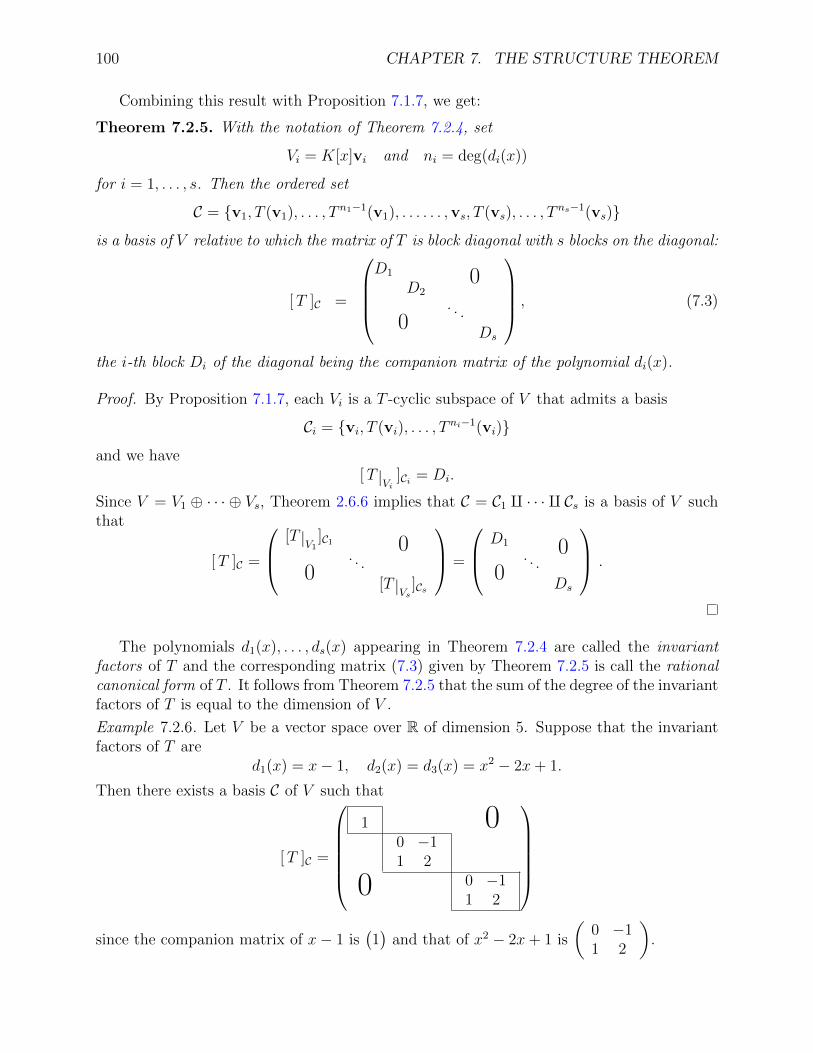
100 CHAPTER 7. THE STRUCTURE THEOREM
Combining this result with Proposition 7.1.7, we get:
Theorem 7.2.5. With the notation of Theorem 7.2.4, set
Vi = K[x]vi and ni = deg(di(x))
for i = 1, . . . , s. Then the ordered set
C = {v1, T (v1), . . . , T n1−1(v1), . . . . . . ,vs, T (vs), . . . , Tns−1(vs)}
is a basis of V relative to which the matrix of T is block diagonal with s blocks on the diagonal:
[T ]C =
D1
D20
0. . .
Ds
, (7.3)
the i-th block Di of the diagonal being the companion matrix of the polynomial di(x).
Proof. By Proposition 7.1.7, each Vi is a T -cyclic subspace of V that admits a basis
Ci = {vi, T (vi), . . . , Tni−1(vi)}
and we have[T |Vi ]Ci = Di.
Since V = V1 ⊕ · · · ⊕ Vs, Theorem 2.6.6 implies that C = C1 q · · · q Cs is a basis of V suchthat
[T ]C =
[T |V1 ]C1 0
0. . .
[T |Vs ]Cs
=
D1 00
. . .
Ds
.
The polynomials d1(x), . . . , ds(x) appearing in Theorem 7.2.4 are called the invariantfactors of T and the corresponding matrix (7.3) given by Theorem 7.2.5 is call the rationalcanonical form of T . It follows from Theorem 7.2.5 that the sum of the degree of the invariantfactors of T is equal to the dimension of V .
Example 7.2.6. Let V be a vector space over R of dimension 5. Suppose that the invariantfactors of T are
d1(x) = x− 1, d2(x) = d3(x) = x2 − 2x+ 1.
Then there exists a basis C of V such that
[T ]C =
1 0
0 −11 2
0 0 −11 2
since the companion matrix of x− 1 is
(1)
and that of x2 − 2x+ 1 is
(0 −11 2
).

7.2. MODULES OVER A EUCLIDEAN DOMAIN 101
The proof of Theorem 7.2.5 does not use the divisibility relations relating the polynomialsd1(x), . . . , ds(x). In fact, it applies to any decomposition of the form (7.2).
Example 7.2.7. Let V be a vector space over C of dimension 5 and let T : V → V be a linearoperator on C. Suppose that, for the corresponding structure of a C[x]-module on V , wehave
V = C[x]v1 ⊕ C[x]v2 ⊕ C[x]v3
and that the monic generators of the annihilators of v1,v2 and v3 are respectively
x2 − i x+ 1− i, x− 1 + 2i, x2 + (2 + i)x− 3.
Then C = {v1, T (v1),v2,v3, T (v3)} is a basis of V and
[T ]C =
0 −1 + i1 i
01− 2i
0 0 31 −2− i
.
Exercises.
7.2.1. Prove Corollary 7.2.2 using Theorem 7.2.1.
7.2.2. Prove Theorem 7.2.3 using Theorem 7.2.1 and Corollary 7.2.2.
7.2.3. Prove Theorem 7.2.4 using Theorem 7.2.1 and Corollary 7.2.2.
7.2.4. Let V be a finite-dimensional real vector space equipped with an endomorphism T ∈EndR(V ). Suppose that, for the corresponding structure of an R[x]-module on V , we have
V = R[x]v1 ⊕ R[x]v2 ⊕ R[x]v3,
where v1, v2 and v3 are elements of V whose respective annihilators are generated by x2 −x + 1, x3 and x − 2. Determine the dimension of V , a basis C of V associated to thisdecomposition and, for this basis, determine [T ]C.
7.2.5. Let A ∈ Matn×n(K) where K is a field. Show that there exist nonconstant monicpolynomials d1(x), . . . , ds(x) ∈ K[x] with d1(x) | · · · | ds(x) and an invertible matrix P ∈Matn×n(K) such that PAP−1 is block diagonal, with the companion matrices of d1(x), . . . , ds(x)on the diagonal.

102 CHAPTER 7. THE STRUCTURE THEOREM
7.3 Primary decomposition
Theorem 7.2.1 tells us that every module of finite type over a euclidean ring is a direct sum ofcyclic submodules. To obtain a finer decomposition, it suffices to decompose cyclic modules.This is the subject of primary decomposition. Since it applies to every module with nonzeroannihilator, we consider the more general case, which is no more complicated.
Before stating the principal result, recall that, if M is a module over a commutative ringA, then, for each a ∈ A, we define A-submodules of M by setting
Ma := {u ∈M ; au = 0} and aM = {au ; u ∈M}
(see Example 6.5.12).
Theorem 7.3.1. Let M be a module over a euclidean ring A. Suppose that M 6= {0} andthat Ann(M) contains a nonzero element a. Write
a = εq1 . . . qs
where ε is a unit in A, s is an integer ≥ 0, and q1, . . . , qs are nonzero elements of A whichare pairwise relatively prime. Then the integer s is ≥ 1 and we have:
1) M = Mq1 ⊕ · · · ⊕Mqs ,
2) Mqi = q1 · · · qi · · · qsM for i = 1, . . . , s.
Furthermore, if Ann(M) = (a), then Ann(Mqi) = (qi) for i = 1, . . . , s.
In formula 2), the hat on qi indicates that qi is omitted from the product. If s = 1, thisproduct is empty and we adopt the convention that q1 · · · qi · · · qs = 1.
Proof. Since Ann(M) is an ideal of A, it contains
ε−1a = q1 · · · qs.
Furthermore, since M 6= {0}, it does not contain 1. Therefore, we must have s ≥ 1.
If s = 1, we find that M = Mq1 = q1M , and formulas 1) and 2) are verified. Supposenow that s ≥ 2 and define
ai := q1 · · · qi · · · qs for i = 1, . . . , s.
Since q1, . . . , qs are pairwise relatively prime, the products a1, . . . , as are relatively prime (i.e.their gcd is one), and so there exist r1, . . . , rs ∈ A such that
r1a1 + · · ·+ rsas = 1
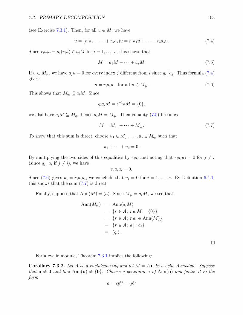
7.3. PRIMARY DECOMPOSITION 103
(see Exercise 7.3.1). Then, for all u ∈M , we have:
u = (r1a1 + · · ·+ rsas)u = r1a1u+ · · ·+ rsasu. (7.4)
Since riaiu = ai(riu) ∈ aiM for i = 1, . . . , s, this shows that
M = a1M + · · ·+ asM. (7.5)
If u ∈Mqi , we have aju = 0 for every index j different from i since qi | aj. Thus formula (7.4)gives:
u = riaiu for all u ∈Mqi . (7.6)
This shows that Mqi ⊆ aiM . Since
qiaiM = ε−1aM = {0},
we also have aiM ⊆Mqi , hence aiM = Mqi . Then equality (7.5) becomes
M = Mq1 + · · ·+Mqs . (7.7)
To show that this sum is direct, choose u1 ∈Mq1 , . . . , us ∈Mqs such that
u1 + · · ·+ us = 0.
By multiplying the two sides of this equalities by riai and noting that riaiuj = 0 for j 6= i(since qj | ai if j 6= i), we have
riaiui = 0.
Since (7.6) gives ui = riaiui, we conclude that ui = 0 for i = 1, . . . , s. By Definition 6.4.1,this shows that the sum (7.7) is direct.
Finally, suppose that Ann(M) = (a). Since Mqi = aiM , we see that
Ann(Mqi) = Ann(aiM)
= {r ∈ A ; r aiM = {0}}= {r ∈ A ; r ai ∈ Ann(M)}= {r ∈ A ; a | r ai}= (qi).
For a cyclic module, Theorem 7.3.1 implies the following:
Corollary 7.3.2. Let A be a euclidean ring and let M = Au be a cylic A-module. Supposethat u 6= 0 and that Ann(u) 6= {0}. Choose a generator a of Ann(u) and factor it in theform
a = εpe11 · · · pess

104 CHAPTER 7. THE STRUCTURE THEOREM
where ε is a unit of A, s is an integer ≥ 1, p1, . . . , ps are pairwise non-associated irreducibleelements of A, and e1, . . . , es are positive integers. Then, for i = 1, . . . , s, the product
ui = pe11 · · · peii · · · pess u ∈M
satisfies Ann(ui) = (peii ), and we have:
M = Au1 ⊕ · · · ⊕ Aus. (7.8)
Proof. Since Ann(M) = Ann(u) = (a), Theorem 7.3.1 applies with q1 = pe11 , . . . , qs = pess .Since
q1 · · · qi · · · qsM = Aui (1 ≤ i ≤ s),
it gives the decomposition (7.8) and
Ann(ui) = Ann(Aui) = (qi) = (peii ) (1 ≤ i ≤ s).
Combining this result with Theorem 7.2.1, we obtain:
Theorem 7.3.3. Let M be a module of finite type over a euclidean ring. Suppose thatM 6= {0} and that Ann(M) 6= {0}. Then M is a direct sum of cyclic submodules whoseannihilator is generated by a power of an irreducible element of A.
Proof. Corollary 7.3.2 shows that the result is true for a cylic module. The general casefollows since, according to Theorem 7.2.1, the module M is a direct sum of cyclic submodules,and the annihilator of each of these submodules is nonzero since it contains Ann(M).
Example 7.3.4. We use the notation of Example 7.1.9. The vector space V is a cyclic Q[x]-module generated by the vector v1 and the ideal Ann(v1) is generated by
p(x) = x3 − x2 + 2x− 2 = (x− 1)(x2 + 2).
Since x2 + 2 has no real root, it has no root in Q, hence it is an irreducible polynomial inQ[x]. The polynomial x − 1 is also irreducible, since its degree is 1. Then Corollary 7.3.2gives
V = Q[x]u1 ⊕Q[x]u2
whereu1 = (x2 + 2)v1 = T 2(v1) + 2v1 = 3v1 + 3v3,
u2 = (x− 1)v1 = T (v1)− v1 = v1 + v2 + v3
satisfyAnn(u1) = (x− 1) and Ann(u2) = (x2 + 2).
Reasoning as in the proof of Theorem 7.2.5, we deduce that
C = {u1,u2, T (u2)} = {3v1 + 3v3,v1 + v2 + v3,−v1 − v2 + 2v3)}

7.3. PRIMARY DECOMPOSITION 105
is a basis of V such that
[T ]C =
1 0
0 0 −21 0
are block diagonal with the companion matrices of x− 1 and x2 + 2 on the diagonal.
We leave it to the reader to analyze the meaning of Theorem 7.3.3 for abelian groups.For the situation that interests us the most, we have:
Theorem 7.3.5. Let V be a finite-dimensional vector space over a field K and let T : V → Vbe a linear operator on V . There exists a basis of V relative to which the matrix of T is blockdiagonal with the companion matrices of powers of monic irreducible polynomials of K[x] onthe diagonal.
This matrix is called a primary rational canonical form of T . We can show that it isunique up to a permutation of the blocks on the diagonal. The powers of monic irreduciblepolynomials whose companion matrices appear on its diagonal are called the elementarydivisors of T .
We leave the proof of this result as an exercise and we give an example.
Example 7.3.6. Let V be a vector space of dimension 6 over R and let T : V → V be a linearoperator. Suppose that, for the corresponding structure of an R[x]-module on V , we have
V = R[x]v1 ⊕ R[x]v2
with Ann(v1) = (x3 − x2) and Ann(v2) = (x3 − 1).
1st We have x3 − x2 = x2(x− 1) where x and x− 1 are irreducible. Thus,
R[x]v1 = R[x]v′1 ⊕ R[x]v′′1
where v′1 = (x− 1)v1 = T (v1)− v1 and v′′1 = x2v1 = T 2(v1) satisfy
Ann(v′1) = (x2) and Ann(v′′1) = (x− 1).
2nd Similarly, x3 − 1 = (x − 1)(x2 + x + 1) is the factorization of x3 − 1 as a product ofpowers of irreducible polynomials of R[x]. Therefore,
R[x]v2 = R[x]v′2 ⊕ R[x]v′′2
where v′2 = (x2 + x+ 1)v2 = T 2(v2) + T (v2) + v2 and v′′2 = (x− 1)v2 = T (v2)− v2
satisfy
Ann(v′2) = (x− 1) and Ann(v′′2) = (x2 + x+ 1).

106 CHAPTER 7. THE STRUCTURE THEOREM
3rd We conclude thatV = R[x]v′1 ⊕ R[x]v′′1 ⊕ R[x]v′2 ⊕ R[x]v′′2
and thatC = {v′1, T (v′1),v′′1 ,v
′2,v
′′2 , T (v′′2)}
is a basis of V for which
[T ]C =
0 01 0
01
1
0 0 −11 −1
,
with the companion matrices of x2, x− 1, x− 1 and x2 + x+ 1 on the diagonal.
Exercises.
7.3.1. Let A be a euclidean domain, let p1, . . . , ps be non-associated irreducible elements ofA and let e1, . . . , es be positive integers. Set qi = peii and ai = q1 · · · qi · · · qs for i = 1, . . . , s.Show that there exists r1, . . . , rs ∈ A such that 1 = r1a1 + · · ·+ rsas.
7.3.2. Let M be a module over a euclidean ring A. Suppose that Ann(M) = (a) with a 6= 0,and that c ∈ A with c 6= 0. Show that Mc = Md where d = gcd(a, c).
7.3.3. Let V be a vector space over a field K and let T ∈ EndK(V ). We consider V as aK[x]-module in the usual way. Show that, in this context, the notions of the submodulesMa and aM introduced in Example 6.5.12 and recalled before Theorem 7.3.1 become:
Vp(x) = ker(p(T )) and p(x)V = Im(p(T ))
for all p(x) ∈ k[x]. Deduce that ker(p(T )) and Im(p(T )) are T -invariant subspaces of V .
7.3.4. Let V be a finite-dimensional vector space over a field K and let T ∈ EndK(V ).Suppose that p(x) ∈ K[x] is a monic polynomial such that p(T ) = 0, and write p(x) =p1(x)e1 · · · ps(x)es where p1(x), . . . , ps(x) are distinct monic irreducible polynomials of K[x]and e1, . . . , es are positive integers. Combining Exercise 7.3.3 and Theorem 7.3.1, show that
(i) V = (ker p1(T )e1)⊕ · · · ⊕ (ker ps(T )es) ,
(ii) ker pi(T )ei = Im(p1(T )e1 . . . pi(T )ei . . . ps(T )es
)for i = 1, . . . s.

7.3. PRIMARY DECOMPOSITION 107
7.3.5. Let V be a vector space of dimension n over a field K, and let T ∈ EndK(V ). Showthat T is diagonalizable if and only if its minimal polynomial minT (x) admits a factorizationof the form
minT (x) = (x− α1) · · · (x− αs)
where α1, . . . , αs are distinct elements of K.
7.3.6. Let T : R3 → R3 be a linear maps whose matrix relative to the standard basis C of R3
is
[T ]C =
2 2 −11 3 −12 4 −1
.
(i) Show that p(T ) = 0 where p(x) = (x− 1)(x− 2) ∈ R[x].
(ii) Why can we assert that R3 = ker(T − I)⊕ ker(T − 2I) ?
(iii) Find a basis B1 for ker(T − I) and a basis B2 for ker(T − 2I).
(iv) Give the matrix of T with respect to the basis B = B1
∐B2 of R3.
7.3.7. Let V be a vector space over Q with basis A = {v1,v2,v3}, and let T : V → V be thelinear map whose matrix relative to the basis A is
[T ]A =
5 1 5−3 −2 −2−3 −1 −3
.
(i) Show that p(T ) = 0 where p(x) = (x+ 1)2(x− 2) ∈ Q[x].
(ii) Why can we assert that V = ker(T + I)2 ⊕ ker(T − 2I) ?
(iii) Find a basis B1 for ker(T + I)2 and a basis B2 for ker(T − 2I).
(iv) Give the matrix of T with respect to the basis B = B1
∐B2 of V .
7.3.8. Let V be a finite-dimensional vector space over C and let T : V → V be a C-linearmap. Suppose that the polynomial p(x) = x4−1 satisfies p(T ) = 0. Factor p(x) as a productof powers of irreducible polynomials in C[x] and give a corresponding decomposition of V asa direct sum of T -invariant subspaces.
7.3.9. Let V be a finite-dimensional vector space over R and let T : V → V be an R-linearmap. Suppose that the polynomial p(x) = x3 + 2x2 + 2x + 4 satisfies p(T ) = 0. Factorp(x) as a product of powers of irreducible polynomials in R[x] and give a correspondingdecomposition of V as a direct sum of T -invariant subspaces.

108 CHAPTER 7. THE STRUCTURE THEOREM
7.3.10 (Application to differential equations). Let D be the operator of derivation on thevector space C∞(R) of infinitely differentiable functions from R to R. Rolle’s Theorem tellsus that if a function f : R → R is differentiable at each point x ∈ R with f ′(x) = 0, then fis constant.
(i) Let λ ∈ R. Suppose that a function satisfies f ′(x) = λf(x) for all x ∈ R. ApplyingRolle’s Theorem to the function f(x)e−λx, shows that there exists a constant C ∈ Rsuch that f(x) = Ceλx for all x ∈ R. Deduce that ker(D − λI) = 〈eλx〉R.
(ii) Let λ1, . . . , λs be distinct real numbers, and let p(x) = (x − λ1) · · · (x − λs) ∈ R[x].Combining the result of (i) with Theorem 7.3.1, show that ker p(D) is a subspace ofC∞(R) of dimension s that admits the basis {eλ1x, . . . , eλsx}.
(iii) Determine the general form of functions f ∈ C∞(R) such that f ′′′ − 2f ′′ − f ′ + 2f = 0.
7.4 Jordan canonical form
In this section, we fix a finite-dimensional vector space V over C and a linear operatorT : V → V . We also equip V with the corresponding structure of a C[x]-module.
Since the irreducible monic polynomials of C[x] are of the form x − λ with λ ∈ C,Theorem 7.3.3 gives
V = C[x]v1 ⊕ · · · ⊕ C[x]vs
for the elements v1, . . . ,vs of V whose annihilators are of the form
Ann(v1) =((x− λ1)e1
), . . . , Ann(vs) =
((x− λs)es
)with λ1, . . . , λs ∈ C and e1, . . . , es ∈ N>0.
Set Ui = C[x]vi for i = 1, . . . , s. For each i, Proposition 7.1.7 shows that Ci :={vi, T (vi), . . . , T
ei−1(vi)} is a basis of Ui and that [T |Ui]Ci is the companion matrix of
(x − λi)ei . Then Theorem 2.6.6 tells us that C = C1 q · · · q Cs is a basis of V relative
to which the matrix [T ]C of T is block diagonal with the companion matrices of the poly-nomials (x− λ1)e1 , . . . , (x− λs)es on the diagonal. This is the rational canonical form of T .The following lemma proposes a different choice of basis for each of the subspaces Ui.
Lemma 7.4.1. Let v ∈ V and let U := C[x]v. Suppose that Ann(v) = ((x−λ)e) with λ ∈ Cand e ∈ N>0. Then
B = {(T − λI)e−1(v), . . . , (T − λI)(v),v}is a basis of U for which
[T |U ]B =
λ 1
λ . . .0
0 . . . 1λ
(7.9)

7.4. JORDAN CANONICAL FORM 109
Proof. Since Ann(v) = ((x− λ)e), Proposition 7.1.7 shows that
C := {v, T (v), . . . , T e−1(v)}
is a basis of U and therefore dimC(U) = e. Set
ui = (T − λI)e−i(v) for i = 1, . . . , e,
so that B can be written asB = {u1,u2, . . . ,ue}
(we adopt the convention that ue = (T − λI)0(v) = v). We see that
T (u1) = (T − λI)(u1) + λu1 = (T − λI)e(v) + λu1 = λu1 (7.10)
since (T − λI)e(v) = (x− λ)ev = 0. For i = 2, . . . , e, we also have
T (ui) = (T − λI)(ui) + λui = ui−1 + λui . (7.11)
Relation (7.10) and (7.11) show in particular that
T (ui) ∈ 〈u1, . . . ,ue〉C for i = 1, . . . , e.
Thus 〈u1, . . . ,ue〉C is a T -invariant subspace of U . Since it contains v = ue, it contains allelements of C and so
〈u1, . . . ,ue〉C = U.
Since dimC(U) = e = |B|, we conclude that B is a basis of U . From (7.10) and (7.11), wededuce
[T (u1)]B = [λu1]B =
λ0...0
and [T (ui)]B = [ui−1 + λui]B =
0...1λ...0
← ifor i = 2, . . . , e,
and hence the form (7.9) for the matrix [T |U ]B.
Definition 7.4.2 (Jordan block). For each λ ∈ C and each e ∈ N>0, we denote by Jλ(e)the square matrix of size e with entries on the diagonal equal to λ, entries just above thediagonal equal to 1, and all other entries equal to 0:
Jλ(e) =
λ 1
λ . . .0
0 . . . 1λ
∈ Mate×e(C).
We call it the Jordan block of size e× e for λ.

110 CHAPTER 7. THE STRUCTURE THEOREM
Thanks to Lemma 7.4.1 and the discussion preceding it, we conclude:
Theorem 7.4.3. There exists a basis B of V such that [T ]B is block diagonal with Jordanblocks on the diagonal.
Proof. Lemma 7.4.1 shows that, for i = 1, . . . , s, the subspace Ui admits the basis
Bi = {(T − λiI)ei−1(vi), . . . , (T − λiI)(vi),vi}
and that[T |Ui
]Bi = Jλi(ei).
Then, according to Theorem 2.6.6, the ordered set B := B1 q · · · q Bs is a basis of V forwhich
[T ]B =
Jλ1(e1) 0
Jλ2(e2). . .
0 Jλs(es)
. (7.12)
We say that (7.12)) is a Jordan canonical form (or Jordan normal form) of T . Thefollowing result shows that this form is essentially unique and gives a method for calculatingit:
Theorem 7.4.4. The Jordan canonical forms of T are obtained from one another by apermutation of the Jordan blocks on the diagonal. These blocks are of the form Jλ(e) whereλ is an eigenvalue of T and where e is an integer ≥ 1. For each λ ∈ C and each integerk ≥ 1, we have
dimC ker(T − λI)k =∑e≥1
min(k, e)nλ(e) (7.13)
where nλ(e) denotes the number of Jordan blocks equal to Jλ(e) on the diagonal.
Before proceeding to the proof of this theorem, we first explain how formula (7.13) allowsus to calculate the integers nλ(e) and hence to determine a Jordan canonical form of T . Forthis, we fix λ ∈ C. We note that there exists an integer r ≥ 1 such that nλ(e) = 0 for alle > r and we set
mk = dimC ker(T − λI)k
for k = 1, . . . , r. Then formula (7.13) gives
m1 = nλ(1) + nλ(2) + nλ(3) + · · ·+ nλ(r),
m2 = nλ(1) + 2nλ(2) + 2nλ(3) + · · ·+ 2nλ(r),
m3 = nλ(1) + 2nλ(2) + 3nλ(3) + · · ·+ 3nλ(r),
. . .
mr = nλ(1) + 2nλ(2) + 3nλ(3) + · · ·+ rnλ(r).
(7.14)

7.4. JORDAN CANONICAL FORM 111
From this we deduce
m1 = nλ(1) + nλ(2) + nλ(3) + · · ·+ nλ(r),
m2 −m1 = nλ(2) + nλ(3) + · · ·+ nλ(r),
m3 −m2 = nλ(3) + · · ·+ nλ(r),
. . .
mr −mr−1 = nλ(r).
Therefore, we can recover nλ(1), . . . , nλ(r) from the data m1, . . . ,mr. Explicitly, this gives
nλ(e) =
2m1 −m2 if e = 1,
2me −me−1 −me+1 if 1 < e < r,
mr −mr−1 if e = r.
(7.15)
Proof of Theorem 7.4.4. Suppose that [T ]B is in Jordan canonical form 7.12 for a basis Bof V .
Exercise 7.4.1 at the end of this section shows that, for every permuation J ′1, . . . , J′s of
the blocks Jλ1(e1), . . . , Jλs(es), there exists a basis B′ of V such that
[T ]B′ =
J ′1 00
. . .
J ′s
.
To prove the first statement of the theorem, it therefore suffices to verify formula (7.13)because, as the remark following the theorem shows, this formula allows us to calculate allthe integers nλ(e) and thus determine a Jordan canonical form of T up to a permutation ofthe blocks on the diagonal.
Fix λ ∈ C and k ∈ N>0, and set n = dimC(V ). We have
dimC ker(T − λI)k = n− rank[(T − λI)k]B
= n− rank([T ]B − λI)k
= n− rank
Jλ1(e1)− λI 00
. . .
Jλs(es)− λI
k
= n− rank
(Jλ1(e1)− λI)k 00
. . .
(Jλs(es)− λI)k
= n−
(rank(Jλ1(e1)− λI)k + · · ·+ rank(Jλs(es)− λI)k
).
Since we also have n = e1 + · · ·+ es, we conclude that
dimC ker(T − λI)k =s∑i=1
(ei − rank(Jλi(ei)− λI)k
).

112 CHAPTER 7. THE STRUCTURE THEOREM
For i = 1, . . . , s, we have
Jλi(ei)− λI =
λi − λ 1
λi − λ . . .0
0 . . . 1λi − λ
= Jλi−λ(ei)
and so the formula becomes
dimC ker(T − λI)k =s∑i=1
(ei − rank(Jλi−λ(ei))
k). (7.16)
If λi 6= λ, we havedet(Jλi−λ(ei)) = (λi − λ)ei 6= 0,
hence Jλi−λ(ei) is invertible. Then Jλi−λ(ei)k is also invertible for each integer k ≥ 1.
Therefore, we haverank(Jλi−λ(ei)
k) = ei if λi 6= λ. (7.17)
If λi = λ, we have
Jλi−λ(ei) = J0(ei) =
0 1
0 . . .0
0 . . . 10
and we easily check by induction on k that
J0(ei)k =
(0 Iei−k
0k 0
)for k = 1, . . . , ei − 1 (7.18)
and that J0(ei)k = 0 if k ≥ ei (in formula (7.18)), the symbol Iei−k represents the identity
matrix of size (ei− k)× (ei− k), the symbol 0k represents the zero matrix of size k× k, andthe symbols 0 on the diagonal are zero matrices of mixed size). From this we deduce that
rank(J0(ei)k) =
{ei − k if 1 ≤ k < ei,
0 if k ≥ ei.(7.19)
By (7.17) and (7.19), formula (7.16) becomes
dimC ker(T − λI)k =∑
{i ;λi=λ}
min(k, ei) =∑e≥1
min(k, e)nλ(e)
where, for each integer e ≥ 1, the integer nλ(e) represents the number of indices i ∈ {1, . . . , s}such that (λi, ei) = (λ, e), hence the number of blocks equal to Jλ(e) on the diagonal of (7.12).This proves formula (7.13) and, at the same time, we complete the proof of the first assertionof the theorem. The exercises at the end of this section propose an alternative proof of (7.13).

7.4. JORDAN CANONICAL FORM 113
Finally, we find that
charT (x) = det(xI − [T ]B) =
∣∣∣∣∣∣∣xI − Jλ1(e1) 0
0. . .
xI − Jλs(es)
∣∣∣∣∣∣∣= det(xI − Jλ1(e1)) · · · det(xI − Jλs(es))= (x− λ1)e1 · · · (x− λs)es .
Thus, the numbers λ for which the Jordan canonical form (7.12) of T contains a block Jλ(e)with e ≥ 1 are the eigenvalues of T . This proves the second assertion of the theorem andcompletes the proof.
To determine the integers nλ(e) using formulas (7.14), we must determine, for each eigen-value λ of T , the largest integer r such that nλ(r) ≥ 1. The following corollary provides amethod for calculating this integer.
Corollary 7.4.5. Let λ be an eigenvalue of T . Let mk = dimC ker(T − λI)k for all k ≥ 1.Then we have
m1 < m2 < · · · < mr = mr+1 = mr+2 = · · ·
where r denotes the largest integer for which nλ(r) ≥ 1.
Proof. Let r be the largest integer for which nλ(r) ≥ 1. The equalities (7.14) show thatmk − mk−1 ≥ nλ(r) ≥ 1 for k = 2, . . . , r and so m1 < m2 < · · · < mr. For k ≥ r,formula (7.13) gives mk = mr.
Example 7.4.6. Let T : C10 → C10 be a linear map. Suppose that its eigenvalues are 1 + iand 2, and that the integers
mk = dimC ker(T − (1 + i)I)k and m′k = dimC ker(T − 2I)k
satisfy
m1 = 3, m2 = 5, m3 = 6, m4 = 6, m′1 = 2, m′2 = 4 and m′3 = 4.
Since m1 < m2 < m3 = m4, Corollary 7.4.5 shows that the largest Jordan block of T for theeigenvalue λ = 1 + i is of size 3×3. Similarly, since m′1 < m′2 = m′3, the largest Jordan blockof T for the eigenvalue λ = 2 is of size 2× 2.
Formulas (7.14) for λ = 1 + i give
m1 = 3 = n1+i(1) + n1+i(2) + n1+i(3),
m2 = 5 = n1+i(1) + 2n1+i(2) + 2n1+i(3),
m3 = 6 = n1+i(1) + 2n1+i(2) + 3n1+i(3),

114 CHAPTER 7. THE STRUCTURE THEOREM
hence n1+i(1) = n1+i(2) = n1+i(3) = 1. For λ = 2, they are written as
m′1 = 2 = n2(1) + n2(2),
m′2 = 4 = n2(1) + 2n2(2),
hence n2(1) = 0 and n2(2) = 2. We conclude that the Jordan canonical form of T is theblock diagonal matrix with the blocks
(1 + i),
(1 + i 1
0 1 + i
),
1 + i 1 00 1 + i 10 0 1 + i
,
(2 10 2
),
(2 10 2
)on the diagonal.
Example 7.4.7. Let T : C4 → C4 be the linear map whose matrix relative to the standardbasis E of C4 is
[T ]E =
1 0 −1 40 1 −1 51 0 −1 81 −1 0 3
.
We wish to determine a Jordan canonical form of T .
Solution: We calculate
charT (x) = det(xI − [T ]E) = x2(x− 2)2.
Thus the eigenvalues of T are 0 and 2. We set
mk = dimC ker(T − 0I)k = 4− rank[T k ]E = 4− rank([T ]E)k
m′k = dimC ker(T − 2I)k = 4− rank[(T − 2I)k]E = 4− rank([T ]E − 2I)k
for every integer k ≥ 1.
We find, after a series of elementary row operations, the following reduced echelon forms:
[T ]E ∼
1 0 −1 00 1 −1 00 0 0 10 0 0 0
[T ]2E =
4 −4 0 84 −4 0 128 −8 0 204 −4 0 8
∼
1 −1 0 00 0 0 10 0 0 00 0 0 0
[T ]3E =
12 −12 0 2016 −16 0 3228 −28 0 5212 −12 0 20
∼
1 −1 0 00 0 0 10 0 0 00 0 0 0

7.4. JORDAN CANONICAL FORM 115
[T ]E − 2I =
−1 0 −1 40 −1 −1 51 0 −3 81 −1 0 1
∼
1 0 0 −10 1 0 −20 0 1 −30 0 0 0
([T ]E − 2I)2 =
4 −4 4 −84 −4 4 −84 −8 8 −120 0 0 0
∼
1 0 0 −10 1 −1 10 0 0 00 0 0 0
([T ]E − 2I)3 =
−8 −12 −12 20−8 −12 −12 20−8 −20 −20 280 0 0 0
=
1 0 0 −10 1 −1 10 0 0 00 0 0 0
hence m1 = 1, m2 = m3 = 2, m′1 = 1 and m′2 = m′3 = 2. So the largest Jordan block of Tfor the eigenvalue 0 is of size 2 × 2 and the block for the eigenvalue 2 is also of size 2 × 2.Since the sum of the sizes of the block must be equal to 4, we conclude that the Jordancanonical form of T is (
J0(2) 00 J2(2)
)=
0 1 0 00 0 0 00 0 2 10 0 0 2
.
However, this does not say how to find a basis B of C4 such that [T ]B is of this form.We will see in the following chapter how to do this in principle.
The matrix version of Theorem 7.4.3 is the following:
Theorem 7.4.8. Let A ∈ Matn×n(C). There exists an invertible matrix P ∈ GLn(C) suchthat P−1AP is block diagonal with Jordan blocks on the diagonal.
Such a product P−1AP =
Jλ1(e1) 00
. . .
Jλs(es)
is called a Jordan canonical form
of A (or Jordan normal form of A).
The matrix version of Theorem 7.4.4 is stated as follows:
Theorem 7.4.9. Let A ∈ Matn×n(C). The Jordan canonical forms of A are obtained fromone another by a permutation of the Jordan blocks on the diagonal. The blocks in questionare of the form Jλ(e) where λ is an eigenvalue of A and where e is an integer ≥ 1. For eachλ ∈ C and each integer k ≥ 1, we have
n− rank(A− λI)k =∑e≥1
min(k, e)nλ(e)
where nλ(e) denotes the number of blocks on the diagonal equal to Jλ(e).

116 CHAPTER 7. THE STRUCTURE THEOREM
This result provides the means to determine if two matrices with complex entries aresimilar or not:
Corollary 7.4.10. Let A,B ∈ Matn×n(C). Then A and B are similar if and only if theyadmit the same Jordan canonical form.
The proof of this statement is left as an exercise.
Exercises.
7.4.1. Let V be a finite-dimensional vector space over C and let T : V → V be a linearoperator. Suppose that there exists a basis B of V such that
[T ]B =
A1 00
. . .
As
where Ai ∈ Matei×ei(C) for i = 1, . . . , s. Write
B = B1 q · · · q Bs
where Bi has ei elements for i = 1, . . . , s. Finally, for each i, denote by Vi the subspace of Vgenerated by Bi.
(a) Show that each subspace Vi is T -invariant, that it admits Bi as a basis and that
[T |Vi ]Bi = Ai.
(b) Show that if (i1, . . . , is) is a permutation of (1, . . . , s), then B′ = Bi1 q· · ·qBis is a basisof V such that
[T ]B′ =
Ai1 00
. . .
Ais
.
7.4.2. Let V be a vector space over C and let T : V → V be a linear operator. Suppose that
V = V1 ⊕ · · · ⊕ Vs
where Vi is a T -invariant subspace of V for i = 1, . . . , s.
(a) Show that ker(T ) = ker(T |V1)⊕ · · · ⊕ ker(T |Vs).

7.4. JORDAN CANONICAL FORM 117
(b) Deduce that, for all λ ∈ C and all k ∈ N>0, we have
ker(T − λIV )k = ker(T |V1 − λIV1)k ⊕ · · · ⊕ ker(T |Vs − λIVs)
k.
7.4.3. Set T : V → V be a linear operator on a vector space V of dimension n over C.Suppose that there exists a basis B = {v1, . . . ,vn} of V and λ ∈ C such that
[T ]B = Jλ(n).
(a) Show that, if λ 6= 0, then dimC(kerT k) = 0 for every integer k ≥ 1.
(b) Suppose that λ = 0. Show that
ker(T k) = 〈v1, . . . ,vk〉C
for k = 1, . . . , n. Deduce that dimC ker(T k) = min(k, n) for every integer k ≥ 1.
7.4.4. Give an alternative proof of formula (7.13) of Theorem 7.4.4 by proceeding in thefollowing manner. First suppose that B is a basis of V such that
[T ]B =
Jλ1(e1) 00
. . .
Jλs(es)
.
By Exercise 7.4.1, we can write B = B1 q · · · q Bs where, for each i, Bi is a basis of aT -invariant subspace Vi of V with
[T |Vi ]Bi = Jλi(ei)
and we have V = V1 ⊕ · · · ⊕ Vs.
(a) Applying Exercise 7.4.2, show that
dimC ker(T − λI)k =s∑i=1
dimC ker(T |Vi − λIVi)k
for each λ ∈ C and each integer k ≥ 1.
(b) Show that [T |Vi − λIVi ]Bi = Jλi−λ(ei) and, using Exercise 7.4.3, deduce that
dimC ker(T |Vi − λIVi)k =
{0 if λ 6= λi ,
min(ei, k) if λ = λi .
(c) Deduce formula (7.13).

118 CHAPTER 7. THE STRUCTURE THEOREM
7.4.5. Deduce Theorem 7.4.8 from Theorem 7.4.3 by applying the latter to the linear operatorTA : Cn → Cn associated to A. Similarly, deduce Theorem 7.4.9 from Theorem 7.4.4.
7.4.6. Prove Corollary 7.4.10.
7.4.7. Let T : C7 → C7 be a linear map. Suppose that its eigenvalues are 0, 1 and −i andthat the integers
mk = dimC kerT k, m′k = dimC ker(T − I)k, m′′k = dimC ker(T + iI)k
satisfy m1 = m2 = 2, m′1 = 1, m′2 = 2, m′3 = m′4 = 3, m′′1 = 1 and m′′2 = m′′3 = 2. Determinea Jordan canonical form of T .
7.4.8. Determine a Jordan canonical form of the matrix
A =
0 1 0−1 0 10 1 0
.

Chapter 8
The proof of the structure theorem
This chapter concludes the first part of the course. We first state a theorem concerningsubmodules of free modules over a euclidean domain and then we show that it implies thestructure theorem for modules of finite type over a euclidean domain. In Section 8.2, weprove the Cayley-Hamilton Theorem which says that, for every linear operator T : V → Von a finite-dimensional vector space V , we have charT (T ) = 0. The rest of the chapter isdedicated to the proof of our submodule theorem. In Section 8.3, we show that, if A is aeuclidean domian, then every submodule N of An has a basis. In Section 8.4, we give analgorithm for finding such a basis from a system of generators of N . In Section 8.5, wepresent a more complex algorithm that allows us to transform every matrix with coefficientsin A into its “Smith normal form” and we deduce from this the theorem on submodules offree modules. Finally, given a linear operator T : V → V as above, Section 8.6 provides amethod for determining a basis B of V such that [T ]B is in rational canonical form.
Throughout this chapter, A denotes a euclidean domain and n is a positive integer.
8.1 Submodules of free modules, Part I
We first state:
Theorem 8.1.1. Let N be an A-submodule of An. Then there exists a basis {C1, . . . , Cn}of An, an integer r with 0 ≤ r ≤ n and nonzero elements d1, . . . , dr of A with d1 | d2 | · · · | drsuch that {d1C1, . . . , drCr} is a basis of N .
The proof of this result is given in Section 8.5. We will see that the elements d1, . . . , drare completely determined by N up to multiplication by units of A. We explain here howwe can deduce the structure theorem for A-modules of finite type from Theorem 8.1.1.
Proof of Theorem 7.2.1. Let M = 〈v1, . . . ,vn〉A be an A-module of finite type. The function
119

120 CHAPTER 8. THE PROOF OF THE STRUCTURE THEOREM
ψ : An −→ Ma1...an
7−→ a1v1 + · · ·+ anvn(8.1)
is a surjective homomorphism of A-modules. Let
N = kerψ.
Then N is an A-submodule of An. By Theorem 8.1.1, there exists a basis {C1, . . . , Cn} ofAn, an integer r with 0 ≤ r ≤ n and nonzero elements d1, . . . , dr of A with d1 | d2 | · · · | drsuch that {d1C1, . . . , drCr} is a basis of N . Then let
ui = ψ(Ci) (i = 1, . . . , n).
Since An = 〈C1, . . . , Cn〉A, we have
M = Im(ψ) = 〈u1, . . . ,un〉A = Au1 + · · ·+ Aun. (8.2)
On the other hand, for a1, . . . , an ∈ A, we find
a1u1 + · · ·+ anun = 0 ⇐⇒ a1ψ(C1) + · · ·+ anψ(Cn) = 0
⇐⇒ ψ(a1C1 + · · ·+ anCn) = 0
⇐⇒ a1C1 + · · ·+ anCn ∈ N.
Recall that {d1C1, . . . , drCr} is a basis of N . Thus the condition a1C1 + · · · + anCn ∈ N isequivalent to the existence of b1, . . . , br ∈ A such that
a1C1 + · · ·+ anCn = b1(d1C1) + · · ·+ br(drCr).
Since C1, . . . , Cn are linearly independent over A, this is not possible unless
a1 = b1d1, . . . , ar = brdr and ar+1 = · · · = an = 0.
We conclude that
a1u1 + · · ·+ anun = 0 ⇐⇒ a1C1 + · · ·+ anCn ∈ N⇐⇒ a1 ∈ (d1), . . . , ar ∈ (dr) and ar+1 = · · · = an = 0.
(8.3)In particular, this shows that
aiui = 0 ⇐⇒
{ai ∈ (di) if 1 ≤ i ≤ r,
ai = 0 if r < i ≤ n.(8.4)
Thus Ann(ui) = (di) for i = 1, . . . , r and Ann(ui) = (0) for i = r + 1, . . . , n. Sinced1 | d2 | · · · | dr, we have
Ann(u1) ⊇ Ann(u2) ⊇ · · · ⊇ Ann(un). (8.5)

8.1. SUBMODULES OF FREE MODULES, PART I 121
Formulas (8.3) and (8.4) also imply that
a1u1 + · · ·+ anun = 0 ⇐⇒ a1u1 = · · · = anun = 0.
By (8.2), this property implies that
M = Au1 ⊕ · · · ⊕ Aun (8.6)
(see Definition 6.4.1). This completes the proof of Theorem 7.2.1 except for the conditionthat Ann(u1) 6= A.
Starting with a decomposition (8.6) satisfying (8.5), it is easy to obtain another withAnn(u1) 6= A. Indeed, for all u ∈M , we have
Ann(u) = A ⇐⇒ u = 0 ⇐⇒ Au = {0}.
Thus if M 6= {0} and k denotes the smallest integer such that uk 6= 0, we have
A 6= Ann(uk) ⊇ · · · ⊇ Ann(un)
andM = {0} ⊕ · · · ⊕ {0} ⊕ Auk ⊕ · · · ⊕ Aun = Auk ⊕ · · · ⊕ Aun
as required. If M = {0}, we obtain an empty direct sum.
Section 8.6 provides an algorithm for determining {C1, . . . , Cn} and d1, . . . , dr as in thestatement of Theorem 8.1.1, provided that we know a system of generators of N . In theapplication of Theorem 7.2.1, this means knowing a system of generators of ker(ψ) where ψis given by (8.1). The following result allows us to find such a system of generators in thesituation most interesting to us.
Proposition 8.1.2. Let V be a vector space of finite dimension n > 0 over a field K,let B = {v1, . . . ,vn} be a basis of V and let T : V → V be a linear operator. For thecorresponding structure of a K[x]-module on V , the function
ψ : K[x]n −→ Vp1(x)...
pn(x)
7−→ p1(x)v1 + · · ·+ pn(x)vn
is a surjective homomorphism of K[x]-modules, and its kernel is the K[x]-submodule of K[x]n
generated by the columns of the matrix xI − [T ]B.
Proof. Write [T ]B = (aij). Let N be the K[x]-submodule of K[x]n generated by the columnsC1, . . . , Cn of xI − [T ]B. For j = 1, . . . , n, we have
Cj =
−a1,j
...x− ajj
...−anj
,

122 CHAPTER 8. THE PROOF OF THE STRUCTURE THEOREM
hence
ψ(Cj) = (−a1j)v1 + · · ·+ (x− ajj)vj + · · ·+ (−anj)vn= T (vj)− (a1jv1 + · · ·+ anjvn)
= 0
and so Cj ∈ ker(ψ). This proves that N ⊆ ker(ψ).
To prove the reverse inclusion, we first show that every n-tuple (p1(x), . . . , pn(x))t ofK[x]n can be written as a sum of an element of N and an element of Kn.
We prove this assertion by induction on the maximum m of the degree of the polynomialsp1(x), . . . , pn(x) where, for the purpose of this argument, we say that the zero polynomial hasdegree 0. If m = 0, then (p1(x), . . . , pn(x))t is an element of Kn and we are done. Supposethat m ≥ 1 and that the result is true for an n-tuple of polynomials of degrees ≤ m − 1.Denoting by bi the coefficient of xm in pi(x), we have:p1(x)
...pn(x)
=
b1xm + (terms of degree ≤ m− 1)
· · · · · ·bnx
m + (terms of degree ≤ m− 1)
= b1xm−1C1 + · · ·+ bnx
m−1Cn︸ ︷︷ ︸∈ N
+
p∗1(x)...
p∗n(x)
for polynomials p∗(x), . . . , p∗n(x) inK[x] of degree≤ m−1. Applying the induction hypothesisto the n-tuple (p∗1(x), . . . , p∗n(x))t, we conclude that (p1(x), . . . , pn(x))t is the sum of anelement of N and an element of Kn.
Let (p1(x), . . . , pn(x))t be an arbitrary element of ker(ψ). By the above observation, wecan write p1(x)
...pn(x)
=
q1(x)...
qn(x)
+
c1...cn
(8.7)
where (q1(x), . . . , qn(x))t ∈ N and (c1, . . . , cn)t ∈ Kn. Since N ⊆ ker(ψ), we see thatc1...cn
=
p1(x)...
pn(x)
−q1(x)
...qn(x)
∈ ker(ψ),
and so, applying ψ to the vector (c1, . . . , cn)t, we get
c1v1 + · · ·+ cnvn = 0.
Since v1, . . . ,vn are linearly independent over K, this implies that c1 = · · · = cn = 0 andequality (8.7) gives p1(x)
...pn(x)
=
q1(x)...
qn(x)
∈ N.

8.1. SUBMODULES OF FREE MODULES, PART I 123
Since the choice of (p1(x), . . . , pn(x))t ∈ ker(ψ) is arbitrary, this shows that ker(ψ) ⊆ N , andso ker(ψ) = N .
Example 8.1.3. Let V be a vector space of dimension 2 over R, let A = {v1,v2} be a basis
of V , and let T ∈ EndR(V ) with [T ]A =
(−1 24 1
). For the corresponding structure of an
R[x]-module over V , we consider the homomorphism of R[x]-modules ψ : R[x]2 → V givenby
ψ
(p1(x)p2(x)
)= p1(x)v1 + p2(x)v2.
(i) By Proposition 8.1.2, ker(ψ) is the submodule of R[x]2 generated by the columns of
xI − [T ]A =
(x+ 1 −2−4 x− 1
),
that is,
ker(ψ) =
⟨(x+ 1−4
),
(−2x− 1
)⟩R[x]
.
(ii) We see that (x2 − 9)v1 = 0 since
(x2 − 9)v1 = T 2(v1)− 9v1 = T (−v1 + 4v2)− 9v1 = 0.
So we have
(x2 − 9
0
)∈ ker(ψ). To write this element of ker(ψ) as a linear combination of
the generators of ker(ψ) found in (i), we proceed as in the proof of Proposition 8.1.2. Weobtain (
x2 − 90
)= x
(x+ 1−4
)+ 0
(−2x− 1
)+
(−x− 9
4x
)and (
−x− 94x
)= (−1)
(x+ 1−4
)+ 4
(−2x− 1
)+
(00
),
thus (x2 − 9
0
)= (x− 1)
(x+ 1−4
)+ 4
(−2x− 1
).

124 CHAPTER 8. THE PROOF OF THE STRUCTURE THEOREM
Exercises.
8.1.1. Let V be a vector space over Q equipped with a basis A = {v1,v2}, and let T ∈
EndQ(V ) with [T ]A =
(1 23 2
). We consider V as a Q[x]-module and we denote by N the
kernel of the homomorphism of Q[x]-modules ψ : Q[x]2 −→ V given by
ψ
(p1(x)p2(x)
)= p1(x) · v1 + p2(x) · v2.
(i) Find a system of generators of N as a Q[x]-module.
(ii) Show that
(x2 − 3−2x− 5
)∈ N and express this column vector as a linear combination of
the generators of N found in (i).
8.1.2. Let V be a vector space over R equipped with a basis A = {v1,v2,v3} an let T ∈
EndR(V ) with [T ]A =
1 2 10 1 20 0 1
. We consider V as a R[x]-module and we denote by N
the kernel of the homomorphism of R[x]-modules ψ : R[x]3 −→ V given by
ψ
p1(x)p2(x)p3(x)
= p1(x) · v1 + p2(x) · v2 + p3(x) · v3.
(i) Find a system of generators of N as a R[x]-module.
(ii) Show that
x2 − x− 6x− 1
x2 − 2x+ 1
∈ N and express this column vector as a linear combination
of the generators of N found in (i).
8.2 The Cayley-Hamilton Theorem
We begin with the following observation:
Proposition 8.2.1. Let N be the A-submodule of An generated by the columns of a matrixU ∈ Matn×n(A). Then N contains det(U)An.

8.2. THE CAYLEY-HAMILTON THEOREM 125
Proof. We know that the adjugate Adj(U) of U is a matrix of Matn×n(A) satisfying
UAdj(U) = det(U)I (8.8)
(see Theorem B.3.4). Denote by C1, . . . , Cn the columns of U and by e1, . . . , en those of I(these are the elements of the standard basis of An). Also write Adj(U) = (aij). Comparingthe j-th columns of the matrices on each side of (8.8), we see that
a1jC1 + · · ·+ anjCn = det(U)ej (1 ≤ j ≤ n).
Since N = 〈C1, . . . , Cn〉A, we deduce that
det(U)An = 〈det(U)e1, . . . , det(U)en〉A ⊆ N.
We can now prove the following fundamental result:
Theorem 8.2.2 (Cayley-Hamilton Theorem). Let V be a finite-dimensional vector spaceover a field K and let T : V → V be a linear operator on V . Then we have
charT (T ) = 0.
Proof. Let B = {v1, . . . ,vn} be a basis of V over K. By Proposition 8.1.2, the kernel of thehomomorphism of K[x]-modules
ψ : K[x]n −→ Vp1(x)...
pn(x)
7−→ p1(x)v1 + · · ·+ pn(x)vn
is the submodule of K[x]n generated by the columns of xI − [T ]B ∈ Matn×n(K[x]). By theproceeding proposition (applied to A = K[x]), this implies that
ker(ψ) ⊇ det(xI − [T ]B) ·K[x]n = charT (x) ·K[x]n.
In particular, for all u ∈ K[x]n, we have charT (x)u ∈ ker(ψ) and so
0 = ψ(charT (x) u) = charT (x)ψ(u).
Since ψ is a surjective homomorphism, this implies that charT (x) ∈ Ann(V ), that is,charT (T ) = 0.
The following consequence is left as an exercise.
Corollary 8.2.3. For every matrix M ∈ Matn×n(K), we have charM(M) = 0.

126 CHAPTER 8. THE PROOF OF THE STRUCTURE THEOREM
Example 8.2.4. For n = 2, we can give a direct proof. Write M =
(a bc d
). We see that
charT (x) =
∣∣∣∣ x− a −b−c x− d
∣∣∣∣ = x2 − (a+ d)x+ (ad− bc)
thus
charM(M) = M2 − (a+ d)M + (ad− bc)I
=
(a2 + bc ab+ bdac+ cd bc+ d2
)− (a+ d)
(a bc d
)+ (ad− bc)
(1 00 1
)=
(0 00 0
).
Exercises.
8.2.1. Prove Corollary 8.2.3.
8.2.2. Let V be a finite-dimensional vector space over a field K and let T : V → V be alinear operator on V .
(i) Show that minT (x) divides charT (x).
(ii) If K = Q and charT (x) = x3 − 2x2 + x, what are the possibilities for minT (x)?
8.2.3 (Alternate proof of the Cayley-Hamilton Theorem). Let V be a vector space of finitedimension n over a field K and let T : V → V be a linear operator on V . The goal of thisexercise is to give another proof of the Cayley-Hamilton Theorem. To do this, we equip Vwith the corresponding structure of a K[x]-module, and we choose an arbitrary element vof V . Let p(x) be the monic generator of Ann(v), and let m be its degree.
(i) Show that there exists a basis B of V such that [T ]B =
(P Q0 R
)where P denotes
the companion matrix of p(x) and where R is a square matrix of size (n−m)×(n−m).
(ii) Show that charT (x) = p(x)charR(x) ∈ Ann(v).
(iii) Why can we conclude that charT (T ) = 0?

8.3. SUBMODULES OF FREE MODULES, PART II 127
8.3 Submodules of free modules, Part II
The goal of this section is to prove the following weaker version of Theorem 8.1.1 as a firststep towards the proof of this theorem.
Theorem 8.3.1. Every A-submodule of An is free and possesses a basis with at most nelements.
This result is false in general for an arbitrary commutative ring A (see Exercise 8.3.1).
Proof. We proceed by induction on n. For n = 1, an A-submodule N of A1 = A is simplyan ideal of A. If N = {0}, then by convention N is free and admits the basis ∅. Otherwise,we know that N = (b) = Ab for a nonzero element b of A since every ideal of A is principal(Theorem 5.4.3). We note that if ab = 0 with a ∈ A then a = 0 since A is an integraldomain. Therefore, in this case, {b} is a basis of N .
Now suppose that n ≥ 2 and that every A-submodule of An−1 admits a basis with atmost n− 1 elements. Let N be an A-submodule of An. We define
I =
a ∈ A ;
aa2...an
∈ N for some a2, . . . , an ∈ A
,
N ′ =
a1
a2...an
∈ N ; a1 = 0
and N ′′ =
a2
...an
∈ An−1 ;
0a2...an
∈ N .
It is straightforward (exercise) to verify that I is an ideal of A, that N ′ is a submodule of Nand that N ′′ is a submodule of An−1. Moreover, the function
ϕ : N ′′ −→ N ′a2...an
7−→
0a2...an
is an isomorphism of A-modules. By the induction hypothesis, N ′′ admits a basis with atmost n − 1 elements. The image of this basis under ϕ is therefore a basis {u1, . . . ,um} ofN ′ with 0 ≤ m ≤ n− 1 (Proposition 6.5.13).
If I = {0}, then we have N = N ′. In this case, {u1, . . . ,um} is a basis of N and, since0 ≤ m ≤ n, we are finished.

128 CHAPTER 8. THE PROOF OF THE STRUCTURE THEOREM
Otherwise, Theorem 5.4.3 implies I = (b1) = Ab1 for a nonzero element b1 of A. Sinceb1 ∈ I, there exists b2, . . . , bn ∈ A such that
um+1 :=
b1
b2...bn
∈ N.We will show that N = N ′ ⊕ Aum+1. Assuming this result, we have that {u1, . . . ,um+1} isa basis of N and, since m+ 1 ≤ n, the induction step is complete.
Let u = (c1, . . . , cn)t ∈ N . By the definition of I, we have c1 ∈ I. Thus there existsa ∈ A such that c1 = a b1. We see that
u− aum+1 =
0
c2 − a b2...
cn − a bn
∈ N ′ ,and so
u = (u− aum+1) + aum+1 ∈ N ′ + Aum+1.
Since the choice of u is arbitrary, this shows that
N = N ′ + Aum+1.
We also note that, for a ∈ A,
aum+1 ∈ N ′ ⇐⇒ a b1 = 0 ⇐⇒ a = 0.
This shows thatN ′ ∩ Aum+1 = {0},
hence N = N ′ ⊕ Aum+1 as claimed.
Example 8.3.2. Let N =
xyz
; 2x+ 3y + 6z = 0
.
(i) Show that N is a Z-submodule of Z3.
(ii) Find a basis of N as a Z-module.
Solution: For (i), it suffices to show that N is a subgroup of Z3. We leave this as an exercise.For (ii), we set
I = {x ∈ Z ; 2x+ 3y + 6z = 0 for some y, z ∈ Z},
N ′ =
xyz
∈ N ; x = 0
and N ′′ =
{(yz
)∈ Z2 ; 3y + 6z = 0
},

8.3. SUBMODULES OF FREE MODULES, PART II 129
as in the proof of Theorem 8.3.1. We see that
3y + 6z = 0 ⇐⇒ y = −2z,
hence
N ′′ =
{(−2zz
); z ∈ Z
}= Z
(−21
)
admits the basis
{(−21
)}and so
u1 :=
0−21
is a basis of N ′. We also see that, for
x ∈ Z, we have
x ∈ I ⇐⇒ 2x = −3y − 6z for some y, z ∈ Z⇐⇒ 2x ∈ (−3,−6) = (3)
⇐⇒ 3 | 2x⇐⇒ 3 |x.
Thus I = (3). Furthermore, 3 is the first component of
u2 =
3−20
∈ N.Repeating the arguments of the proof of Theorem 8.3.1, we see that
N = N ′ ⊕ Zu2 = Zu1 ⊕ Zu2.
Thus
u1 =
0−21
, u2 =
3−20
is a basis of N .
Exercises.
8.3.1. Let A be an arbitrary integral domain and let I be an ideal of A considered as anA-submodule of A1 = A. Show that I is a free A-module if and only I is principal.
8.3.2. Let M be a free module over a euclidean domain A. Show that every A-submodule ofM is free.
8.3.3. Let N =
xyz
∈ Z3 ; 3x+ 10y − 16z = 0
.
(i) Show that N is a submodule of Z3.

130 CHAPTER 8. THE PROOF OF THE STRUCTURE THEOREM
(ii) Find a basis of N as a Z-module.
8.3.4. Let N =
p1(x)p2(x)p3(x)
∈ Q[x]3 ; (x2 − x)p1(x) + x2p2(x)− (x2 + x)p3(x) = 0
.
(i) Show that N is a Q[x]-submodule of Q[x]3.
(ii) Find a basis of N as a Q[x]-module.
8.4 The column module of a matrix
Definition 8.4.1 (Column module). We define the column module of a matrix U ∈ Matn×m(A)to be the A-submodule of An generated by the columns of A. We denote it by ColA(U).
Theorem 8.3.1 shows that every submodule of An has a basis with at most n elements.Thus the column module of a matrix U ∈ Matn×m(A) has a basis. The goal of this sectionis to give an algorithm for finding such a basis. More generally, this algorithm permits us tofind a basis of an arbitrary submodule N of An provided that we know a system of generatorsC1, . . . , Cm of N since N is then the column module of the matrix (C1 · · ·Cm) ∈ Matn×m(A)whose columns are C1, . . . , Cm.
We begin with the following observation:
Lemma 8.4.2. Let U ∈ Matn×m(A) and let U ′ be a matrix obtained from U by applying oneof the following operations:
(I) interchange two columns,
(II) add to one column the product of another column and an element of A,
(III) multiply a column by an element of A×.
Then U and U ′ have the same column module.
Proof. By construction, the columns of U ′ belong to ColA(U) since they are linear com-binations of the columns of U . Thus we have ColA(U ′) ⊆ ColA(U). On the other hand,each of the operations of type (I), (III) or (III) is invertible: we can recover U from U ′ byapplying an operation of the same type. Thus we also have ColA(U) ⊆ ColA(U ′), and soColA(U) = ColA(U ′).
The operations (I), (II), (III) of Lemma 8.4.2 are called elementary column operations(on A). From this lemma we deduce:

8.4. THE COLUMN MODULE OF A MATRIX 131
Lemma 8.4.3. Let U ∈ Matn×m(A) and let U ′ be a matrix obtained from U by applying aseries of elementary column operation. Then ColA(U) = ColA(U ′).
Definition 8.4.4 (Echelon form). We say that a matrix U ∈ Matn×m(A) is in echelon form ifit is in the form
U =
0 0 · · · · · · 0 0 · · · 0...
......
......
0...
......
...
ui1,1... · · · · · · ...
......
∗ 0...
......
... ui2,2...
......
... ∗ 0...
......
... uir,r...
......
... ∗ ......
......
......
...∗ ∗ · · · · · · ∗ 0 0
(8.9)
with 1 ≤ i1 < i2 < · · · < ir ≤ n and ui1,1 6= 0, . . . , uir,r 6= 0.
Lemma 8.4.5. Suppose that U ∈ Matn×m(A) is in echelon form. Then the nonzero columnsof U form a basis of ColA(U).
Proof. Suppose that U is given by (8.9). Then the first r columns C1, . . . , Cr of U generateColA(U). Suppose that we have
a1C1 + · · ·+ arCr = 0
for elements a1, . . . , ar of A. If a1, . . . , ar are not nonzero, there exists a smallest integer ksuch that ak 6= 0. Then we have
akCk + · · ·+ arCr = 0.
Taking the ik-th component of each side of this equality, we see that
akuik,k = 0.
Since ak 6= 0 and uik,k 6= 0, this is impossible (since A is an integral domain). This con-tradiction shows that we must have a1 = · · · = ar = 0. Thus the columns C1, . . . , Cr arelinearly independent and so they form a basis of ColA(U).
The three preceding lemmas only use the fact that A is an integral domain. The followingresult uses in a crucial way the hypothesis that A is a euclidean domain.
Theorem 8.4.6. Let U ∈ Matn×m(A). It is possible to bring U to echelon form by a seriesof elementary column operations.

132 CHAPTER 8. THE PROOF OF THE STRUCTURE THEOREM
Proof. Let ϕ : A \ {0} → N be a euclidean function for A (see Definition 5.4.1). We considerthe following algorithm:
Algorithm 8.4.7.
1. If U = 0, the matrix U is already in echelon form and we are finished.
2. Suppose that U 6= 0. We locate the first nonzerorow of U .
06= 0∗
←2.1. In this row we choose an element a 6= 0 forwhich ϕ(a) is minimal and we permute the columnsto bring this element to the first column.
0a 6= 0 a2 · · · am
∗
2.2. We divide each of the other elements a2, . . . , amof this row by a by writing
aj = qja+ rj
with qj, rj ∈ A satisfying rj = 0 or ϕ(rj) < ϕ(a),then, for j = 2, . . . ,m, we subtract from the j-thcolumn the product of the first column and qj.
C2− q2C1 · · · Cm− qmC1
↓ ↓ 0 a r2 · · · rm∗
2.3. If r2, . . . , rm are not all zero, we return to step2.1.
If they are all zero, the new matrix is in the form pic-tured to the right and we return to step 1, restrictingourselves to the submatrix formed by the last m − 1columns, that is, ignoring the first column.
0 0 · · · · · · 0...
......
0 0 · · · · · · 0a 0 · · · · · · 0∗ ∗
This algorithm terminates after a finite number of steps since each iteration of steps2.1 to 2.3 on a row replaces the first element a 6= 0 of this row by an element a′ 6= 0of A with ϕ(a′) < ϕ(a), and this cannot be repeated indefinitely since ϕ takes values inN = {0, 1, 2, . . . }. When completed, this algorithm produces a matrix in echelon form asrequired.
Combining this theorem with the preceding lemmas, we conclude:
Corollary 8.4.8. Let U ∈ Matn×m(A). By a series of elementary column operations, wecan transform U to a echelon matrix U ′. Then the nonzero columns of U ′ form a basis ofColA(U).
Proof. The first assertion follows from Theorem 8.4.6. By Lemma 8.4.3, we have ColA(U) =ColA(U ′). Finally, Lemma 8.4.5 shows that the nonzero columns of U ′ form a basis ofColA(U ′), hence these also form a basis of ColA(U).

8.4. THE COLUMN MODULE OF A MATRIX 133
Example 8.4.9. Find a basis of ColZ(U) where U =
3 7 4−4 −2 21 −5 −6
∈ Mat3×3(Z).
Solution: We have
U ∼
C2 − 2C1 C3 − C1
3 1 1−4 6 61 −7 −7
∼ C2 C1
1 3 16 −4 6−7 1 −7
∼
C2 − 3C1 C3 − C1
1 0 06 −22 0−7 22 0
∼ −C2
1 0 06 22 0−7 −22 0
.
Thus
1
6−7
,
022−22
is a basis of ColZ(U).
Example 8.4.10. Find a basis of
N :=
⟨(x2 − 1x+ 1
),
(x2 − xx
),
(x3 − 7x− 1
)⟩Q[x]
⊆ Q[x]2.
Solution: We have N = ColQ[x](U) where
U =
(x2 − 1 x2 − x x3 − 7x+ 1 x x− 1
)∼( C2 − C1 C3 − xC1
x2 − 1 −x+ 1 x− 7x+ 1 −1 −x2 − 1
)
∼( C2 C1
−x+ 1 x2 − 1 x− 7−1 x+ 1 −x2 − 1
)∼( −C1
x− 1 x2 − 1 x− 71 x+ 1 −x2 − 1
)
∼( C2 − (x+ 1)C1 C3 − C1
x− 1 0 −61 0 −x2 − 2
)∼( −C3 C1 C2
6 x− 1 0x2 + 2 1 0
)
∼( 6C2
6 6(x− 1) 0x2 + 2 6 0
)since 6 ∈ Q[x]× = Q×,
∼( C2 − (x− 1)C1
6 0 0x2 + 2 −x3 + x2 − 2x+ 8 0
)

134 CHAPTER 8. THE PROOF OF THE STRUCTURE THEOREM
Thus
{(6
x2 + 2
),
(0
−x3 + x2 − 2x+ 8
)}is a basis of N over Q[x].
Exercises.
8.4.1. Find a basis of the subgroup of Z3 generated by
246
and
203
.
8.4.2. Find a basis of the R[x]-submodule of R[x]2 generated by the pairs
(x2 − 1x
),
(x2 − 2x+ 1
x− 2
)and
(x3 − 1x2 − 1
).
8.4.3. Let A be a euclidean domain, and let U ∈ Matn×m(A). Show that the ideal I of Agenerated by the elements of the first row of U is not affected by the elementary columnoperations. Deduce that if a series of elementary column operations transforms U into amatrix whose first row is (a, 0, . . . , 0), then a is a generator of I.
8.5 Smith normal form
To define the notion of elementary row operation on a matrix, we replace everywhere theword “column” by “row” in statements (I) to (III) of Lemma 8.4.2:
Definition 8.5.1 (Elementary row operation). An elementary row operation on a matrix ofMatn×m(A) is any operation of one of the following types:
(I) interchange two rows,
(II) add to one row the product of another row and an element of A,
(III) multiply a row by an element of A×.
To study the effect of an elementary row operation on the column module of a matrix,we will use the following proof whose proof is left as an exercise (see Exercise 6.5.4).
Lemma 8.5.2. Let ϕ : M → M ′ be a homomorphism of A-modules and let N be an A-submodule of M . Then
ϕ(N) := {ϕ(u) ; u ∈M}is an A-submodule of M ′. Furthermore:

8.5. SMITH NORMAL FORM 135
(i) if N = 〈u1, . . . ,um〉A, then ϕ(N) = 〈ϕ(u1), . . . , ϕ(um)〉A;
(ii) if N admits a basis {u1, . . . ,um} and ϕ is injective, then {ϕ(u1), . . . , ϕ(um)} is a basisof ϕ(N).
We can now prove:
Lemma 8.5.3. Let U ∈ Matn×m(A) and let U ′ be a matrix obtained from U by applying anelementary row operation. Then there exists an automorphism ϕ of An such that
ColA(U ′) = ϕ(ColA(U)).
Recall that an automorphism of an A-module is an isomorphism from this module toitself.
Proof. Let C1, . . . , Cm be the columns of U and let C ′1, . . . , C′m be those of U ′. We split the
proof into three cases.
If U ′ is obtained from U by applying an operation of type (I), we will simply assumethat we have interchanged rows 1 and 2. The general case is similar but more complicatedto write. In this case, the function ϕ : An → An given by
ϕ
u1
u2
u3...un
=
u2
u1
u3...un
is an automorphism of An such that ϕ(Cj) = C ′j for j = 1, . . . ,m. Since ColA(U) =〈C1, . . . , Cm〉A and ColA(U ′) = 〈C ′1, . . . , C ′m〉A, Lemma 8.5.2 then gives ColA(U ′) = ϕ(ColA(U ′)).
If U ′ is obtained by an operation of type (II), we will suppose that we have added to row1 the product of row 2 and an element a of A. Then we have C ′j = ϕ(Cj) for j = 1, . . . ,mwhere ϕ : An → An is the function given by
ϕ
u1
u2...un
=
u1 + a u2
u2...un
.
We verify that ϕ is an automorphism of An and the conclusion then follows from Lemma 8.5.2.
Finally, if U ′ is obtained by an operation of type (III), we will suppose that we havemultiplied row 1 of U a unit a ∈ A×. Then C ′j = ϕ(Cj) for j = 1, . . . ,m where ϕ : An → An
is the automorphism of An given by
ϕ
u1
u2...un
=
a u1
u2...un
,

136 CHAPTER 8. THE PROOF OF THE STRUCTURE THEOREM
and Lemma 8.5.2 gives ColA(U ′) = ϕ(ColA(U)).
Combining Lemma 8.4.2 and 8.5.3, we get:
Theorem 8.5.4. Let U ∈ Matn×m(A) and let U ′ be a matrix obtained from U by applyinga series of elementary row and column operations. Then there exists an automorphismϕ : An → An such that
ColA(U ′) = ϕ(ColA(U)).
Proof. By assumption, there exists a series of matrices
U1 = U, U2, U3, . . . , Uk = U ′
such that, for i = 1, . . . , k − 1, the matrix Ui+1 is obtained by applying to Ui an elementaryrow or column operation. In the case of a row operation, Lemma 8.5.3 gives
ColA(Ui+1) = ϕi(ColA(Ui))
for an automorphism ϕi of An. In the case of a column operation, Lemma 8.4.2 gives
ColA(Ui+1) = ColA(Ui) = ϕi(ColA(Ui))
where ϕi = IAn is the identity function on An. We deduce that
ColA(U ′) = ColA(Uk) = ϕk−1(. . . ϕ2(ϕ1(ColA(U1))) . . . ) = ϕ(ColA(U))
where ϕ = ϕk−1 ◦ · · · ◦ ϕ2 ◦ ϕ1 is an automorphism of An.
Theorem 8.5.4 is valid over an arbitrary commutative ring A. Using the assumption thatA is euclidean, we show:
Theorem 8.5.5. Let U ∈ Matn×m(A). Applying to U a series of elementary row and columnoperations, we can bring it to the form
d1 0 00
. . .
dr
0 0
(8.10)
for an integer r ≥ 0 and nonzero elements d1, . . . , dr of A with d1 | d2 | . . . | dr.
We say that (8.10) is the Smith normal form of U . We can show that the elementsd1, . . . , dr are uniquely determined by U up to multiplication by a unit of A (see Exer-cise 8.5.4). We call them the invariant factors of U . The connection to the invariant factorsmentioned after Theorem 7.2.5 is that the invariant factors there are the invariant factors(in the sense of Smith normal form) of the matrix xI −A, where A is the matrix associatedto T in some basis.

8.5. SMITH NORMAL FORM 137
Proof. If U = 0, the matrix U is already in Smith normal form with r = 0. We thereforesuppose that U 6= 0. Then it suffices to show that U can be transformed into a matrix oftype
d 0 · · · 00... U∗
0
(8.11)
where d is a nonzero element of A that divides all the coefficients of U∗.
Since U 6= 0, there exists a nonzero element a of U for which ϕ(a) is minimal. Bypermuting the row and columns of U , we can bring this element to position (1,1):
...· · · a · · ·
...
∼ · · · a · · ·
...
...
∼ a · · · · · ·
...
...
Step 1. Let a2, . . . , am be the other elements of the first row. For j = 2, . . . ,m, we writeaj = qja + rj with qj, rj ∈ A satisfying rj = 0 or ϕ(rj) < ϕ(a), and then we subtract fromcolumn j the product of column 1 and qj. This gives
C2− q2C1 Cm− qmC1a r2 · · · rm
∗... ∗∗
If r1 = · · · = rm = 0 (this happens when a divides all the elements of the first row), thismatrix is of the form
a 0 · · · 0∗... ∗∗
.
Otherwise, we chose an index j with rj 6= 0 for which ϕ(rj) is minimal and we interchangecolumns 1 and j to bring this element rj to position (1, 1). This gives a matrix of the form
a′ ∗ · · · ∗∗... ∗∗
with a′ 6= 0 and ϕ(a′) < ϕ(a). We then repeat the procedure. Since every series of nonzeroelements a, a′, a′′, . . . of A with ϕ(a) > ϕ(a′) > ϕ(a′′) > · · · cannot continue indefinitely, we

138 CHAPTER 8. THE PROOF OF THE STRUCTURE THEOREM
obtain, after a finite number of iterations, a matrix of the formb 0 · · · 0∗... ∗∗
(8.12)
with b 6= 0 and ϕ(b) ≤ ϕ(a). Furthermore, we have ϕ(b) < ϕ(a) if at the start a does notdivide all the elements of row 1.
Step 2. Let b2, . . . , bm be the other elements of the first column of the matrix (8.12). Fori = 2, . . . , n, we write bi = q′ib+ r′i with q′i, r
′i ∈ A satisfying r′i = 0 or ϕ(r′i) < ϕ(b), and then
we subtract from row i row 1 multiplied by q′i. This givesb 0 · · · 0r′2... ∗r′n
R2 − q′2R1...
Rn − q′nR1
If r′2 = · · · = r′n = 0 (this happens when b divides all the elements of the first column), thismatrix is of the form
b 0 · · · 00... ∗0
.
Otherwise we choose an index i with r′i 6= 0 for which ϕ(r′i) is minimal and then withinterchange rows 1 and i to bring this element r′i to position (1, 1). This gives a matrix ofthe form
b′ ∗ · · · ∗∗... ∗∗
with b′ 6= 0 and ϕ(b′) < ϕ(b). We then return to step 1. Since every series of nonzeroelements b, b′, b′′, . . . of A with ϕ(b) > ϕ(b′) > ϕ(b′′) > · · · is necessarily finite, we obtain,after a finite number of steps, a matrix of the form
c 0 · · · 00... U ′
0
(8.13)
with c 6= 0 and ϕ(c) ≤ ϕ(a). Moreover, we have ϕ(c) < ϕ(a) if initially a does not divide allthe elements of the first row and first column.

8.5. SMITH NORMAL FORM 139
Step 3. If c divides all the entries of the submatrix U ′ of (8.13) we have finished. Otherwise,we add to row 1 a row that contains an element of U ′ that is not divisible by c. We thenreturn to step 1 with the resulting matrix
c c2 · · · cm0... U ′
0
R1 +Ri where c - Ri.
Since c does not divides all the entries of row 1 and column 1, this produces a new matrixc′ 0 · · · 00... U ′′
0
with c′ 6= 0 and ϕ(c′) < ϕ(c). Since every series of nonzero elements c, c′, c′′, . . . of A withϕ(c) > ϕ(c′) > ϕ(c′′) > · · · is necessarily finite, we obtain, after a finite number of iterations,a matrix of the required form (8.10) where d 6= 0 divides all the entries of U∗
Example 8.5.6. Find the Smith normal form of U =
(4 8 44 10 8
)∈ Mat2×3(Z).
Solution: The calculation gives:
U ∼( C2 − 2C1 C3 − C1
4 0 04 2 4
)∼(
4 0 00 2 4↑
not divisibleby 4
)R2 −R1
∼(
4 2 40 2 4
)R1 +R2
∼( C2 C1
2 4 42 0 4
)∼( C2 − 2C1 C3 − 2C1
2 0 02 −4 0
)∼(
2 0 00 −4 0
)R2 −R1
∼(
2 0 00 4 0
)−R2
Example 8.5.7. Find the invariant factors of
U =
x 1 13 x− 2 −3−4 4 x+ 5
∈ Mat3×3(Q[x]).

140 CHAPTER 8. THE PROOF OF THE STRUCTURE THEOREM
Solution: We have
U ∼
C2 C1
1 x 1x− 2 3 −3
4 −4 x+ 5
∼
C2 − xC1 C3 − C1
1 0 0x− 2 −x2 + 2x+ 3 −x− 1
4 −4x− 4 x+ 1
∼
1 0 00 −x2 + 2x+ 3 −x− 10 −4x− 4 x+ 1
R2 − (x− 2)R1
R3 − 4R1
∼
C3 C2
1 0 00 −x− 1 −x2 + 2x+ 30 x+ 1 −4x− 4
∼
1 0 00 x+ 1 x2 − 2x− 30 0 −x2 − 2x− 1
−R2
R3 +R2
∼
C3 − (x− 3)C2
1 0 00 x+ 1 00 0 −(x+ 1)2
∼
1 0 00 x+ 1 00 0 (x+ 1)2
−R3
Thus the invariant factors of U are 1, x+ 1 and (x+ 1)2.
We conclude this section with the proof of Theorem 8.1.1:
Proof of Theorem 8.1.1. Let N be a submodule of An. By Theorem 8.3.1, N has a basis,hence in particular it has a finite system of generators {u1, . . . ,um} and thus we can write
N = ColA(U) where U = (u1 · · ·um) ∈ Matn×m(A).
By Theorem 8.5.5, we can, by a series of elementary row and column operations, bring thematrix U to the form
U ′ =
d1 0 00
. . .
dr
0 0
for an integer r ≥ 0 and nonzero elements d1, . . . , dr of A with d1 | d2 | · · · | dr. By Theo-rem 8.5.4, there exists an automorphism ϕ of An such that
ColA(U ′) = ϕ(ColA(U) = ϕ(N).
Denote by {e1, . . . , en} the standard basis of An, and set Cj = ϕ−1(ej) for each j = 1, . . . , n.Since ϕ−1 is an automorphism of An, Proposition 6.5.13 shows that {C1, . . . , Cn} is a basisof An. Also, we know, thanks to Lemma 8.4.5, that {d1e1, . . . , drer} is a basis of ColA(U ′).Then Lemma 8.5.2 applied to ϕ−1 tells us that
{ϕ−1(d1e1), . . . , ϕ−1(drer)} = {d1C1, . . . , drCr}
is a basis of ϕ−1(ColA(U ′)) = N.

8.6. ALGORITHMS 141
Exercises.
8.5.1. Prove Lemma 8.5.2.
8.5.2. Find the invariant factors of each of the following matrices:
(i)
6 4 02 0 32 2 8
∈ Mat3×3(Z), (ii)
(9 6 123 0 4
)∈ Mat2×3(Z),
(iii)
x3 0 x2
x2 x 00 x x3
∈ Mat3×3(Q[x]), (iv)
(x3 − 1 0 x4 − 1x2 − 1 x+ 1 0
)∈ Mat2×3(Q[x]).
8.5.3. Let A be a euclidean domain and let U ∈ Matn×m(A). Show that the ideal I of Agenerated by all the entries of U is not affected by elementary row or column operations.Deduce that the first invariant factor of U is a generator of I and that therefore this divisoris uniquely determined by U up to multiplication by a unit.
8.5.4. Let A and U be as in Exercise 8.5.3, and let k be an integer with 1 ≤ k ≤ min(n,m).For all integers i1, . . . , ik and j1, . . . , jk with
1 ≤ i1 < i2 < · · · < ik ≤ n and 1 ≤ j1 < j2 < · · · < jk ≤ m,
we denote by U j1,...,jki1,...,ik
the submatrix of U of size k× k formed by the entries of U appearingin the rows with indices i1, . . . , ik and the columns with indices j1, . . . , jk. Let Ik be the idealof A generated by the determinants of all these submatrices (called the k× k minors of U).
(i) Show that this ideal is not affected by elementary row or column operations.
(ii) Let d1, . . . , dr be the invariant factors of U . Deduce from (i) that Ik = (d1 · · · dk) ifk ≤ r and that Ik = (0) if k > r.
(iii) Conclude that the integer r is the greatest integer for which U contains a submatrix ofsize r × r with nonzero determinant, and that the invariant factors d1, . . . , dr of U areuniquely determined by U up to multiplication by units in A×.
Note. This construction generalizes that of Exercise 8.5.3 since I1 is simply the ideal of Agenerated by all the elements of U .
8.6 Algorithms
The proof of Theorem 8.1.1 given in the preceding section gives, in principle, a method offinding the basis {C1, . . . , Cn} of An appearing in the statement of the theorem. The goal ofthis section is to give a practical algorithm to achieve this goal, then to deduce an algorithmfor calculating the rational canonical form of an endomorphism of a finite-dimensional vectorspace. We begin with the following observation:

142 CHAPTER 8. THE PROOF OF THE STRUCTURE THEOREM
Lemma 8.6.1. Let U ∈ Matn×m(A), let U ′ be a matrix obtaining by applying to U anelementary column operation, and let E be the matrix obtained by applying the same operationto Im (the m×m identity matrix). Then we have:
U ′ = U E.
Proof. Denote the columns of U by C1, . . . , Cm. We split the proof into three cases:
(I) The matrix U ′ is obtained by interchanging columns i and j of U , where i < j. Wethen have
U ′ = (C1 · · ·i∨Cj · · ·
j∨Ci · · ·Cm)
= (C1 · · ·Ci · · ·Cj · · ·Cm)
i j↓ ↓
1
. . .
10 · · · 1 ← i...
. . ....
1 · · · 0 ← j1
. . .
1
= U E.
(II) The matrix U ′ is obtained by adding to column i of U the product of column j of Uand an element a of A, where j 6= i. In this case
U ′ = (C1 · · ·i∨
Ci + aCj · · ·j∨Cj · · ·Cm)
= (C1 · · ·Ci · · ·Cj · · ·Cm)
1
. . .
1 ← i...
. . .
a · · · 1 ← j. . .
1
= U E.
(This presentation supposes i < j. The case i > j is similar.)
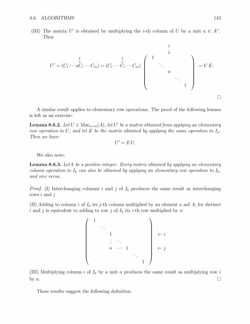
8.6. ALGORITHMS 143
(III) The matrix U ′ is obtained by multiplying the i-th column of U by a unit a ∈ A×.Then
U ′ = (C1 · · ·i∨aCi · · ·Cm) = (C1 · · ·
i∨Ci · · ·Cm)
i↓
1
. . .
a. . .
1
= U E.
A similar result applies to elementary row operations. The proof of the following lemmais left as an exercise:
Lemma 8.6.2. Let U ∈ Matn×m(A), let U ′ be a matrix obtained from applying an elementaryrow operation to U , and let E be the matrix obtained by applying the same operation to In.Then we have:
U ′ = E U.
We also note:
Lemma 8.6.3. Let k be a positive integer. Every matrix obtained by applying an elementarycolumn operation to Ik can also be obtained by applying an elementary row operation to Ik,and vice versa.
Proof. (I) Interchanging columns i and j of Ik produces the same result as interchangingrows i and j
(II) Adding to column i of Ik its j-th column multiplied by an element a aof A, for distincti and j is equivalent to adding to row j of Ik its i-th row multiplied by a:
1
. . .
1 ← i...
. . .
a · · · 1 ← j. . .
1
(III) Multiplying column i of Ik by a unit a produces the same result as multiplying row i
by a.
These results suggest the following definition.

144 CHAPTER 8. THE PROOF OF THE STRUCTURE THEOREM
Definition 8.6.4 (Elementary matrix). A k×k elementary matrix is any matrix of Matk×k(A)obtained by applying an elementary row or column operation to Ik.
We immediately note:
Proposition 8.6.5. An elementary matrix is invertible and its inverse is again an elemen-tary matrix.
Proof. Let E ∈ Matk×k(A) be an elementary matrix. It is obtained by applying to Ik anelementary column operation. Let F be the matrix obtained by applying to Ik the inverseelementary operation. Then Lemma 8.6.1 gives Ik = EF and Ik = FE. Thus E is invertibleand E−1 = F .
Note. The fact that an elementary matrix is invertible can also be seen by observing thatits determinant is a unit of A (see Appendix B).
Using the notion of elementary matrices, we can reformulate Theorem 8.5.5 in the fol-lowing manner:
Theorem 8.6.6. Let U ∈ Matn×m(A). There exist elementary matrices E1, . . . , Es of sizen× n and elementary matrices F1, . . . , Ft of size m×m such that
Es · · ·E1 U F1 · · ·Ft =
d1 0 00
. . .
dr
0 0
(8.14)
for some integer r ≥ 0 and nonzero elements d1, . . . , dr of A with d1 | d2 | · · · | dr.
Proof. Theorem 8.5.5 tells us that we can transform U to a matrix of the form on the rightside of (8.14) by a series of elementary row and column operations. Equality (8.14) followsby denoting by Ei the elementary matrix that encodes the i-th elementary row operationand by Fj the elementary matrix that encodes the j-th elementary column operation.
Since every elementary matrix is invertible and a product of invertible matrices in invert-ible, we deduce:
Corollary 8.6.7. Let U ∈ Matn×m(A). There exists invertible matrices P ∈ Matn×n(A)and Q ∈ Matm×m(A) such that PUQ is in Smith normal form.
To calculate P and Q, we can proceed as follows:
Algorithm 8.6.8. Let U ∈ Matn×m(A).
• We construct the “corner” table
[U In
Im.

8.6. ALGORITHMS 145
• Applying a series of elementary operations to its first n row and its first m columns, we
bring it to the form
[S P
Qwere S denotes the Smith normal form of U .
• Then P and Q are invertible matrices such that PUQ = S.
Proof. Let s be the number of elementary operations needed and, for i = 0, 1, . . . , s, let[Ui Pi
Qi
be the table obtained after i elementary operation, so that the series of intermediate tablesis [
U In
Im=
[U0 P0
Q0
∼
[U1 P1
Q1
∼ · · · ∼
[Us Ps
Qs
=
[S P
Q.
We will show by induction that, for i = 0, 1, . . . , s, the matrices Pi and Qi are invertible andthat PiUQi = Ui. For i = s, this will show that P and Q are invertible with PUQ = S asclaimed.
For i = 0, the statement to prove is clear since In and Im are invertible and InUIm = U .Now suppose that we have 1 ≤ i < s, that Pi−1 and Qi−1 are invertible and that Pi−1UQi−1 =Ui−1. We split into two cases.
Case 1: The i-th operation is an elementary row operation (on the first n rows). In thiscase, if E is the corresponding elementary matrix, we have
Ui = EUi−1, Pi = EPi−1 and Qi = Qi−1.
Since E, Pi−1 and Qi−1 are invertible, we deduce that Pi and Qi are invertible and that
PiUQi = EPi−1UQi−1 = EUi−1 = Ui.
Case 2: The i-th operation is an elementary column operation (on the first m columns).In this case, if F is the corresponding elementary matrix, we have
Ui = Ui−1F, Pi = Pi−1 and Qi = Qi−1F.
Since F , Pi−1 and Qi−1 are invertible, so are Pi and Qi and we obtain
PiUQi = Pi−1UQi−1F = Ui−1F = Ui.

146 CHAPTER 8. THE PROOF OF THE STRUCTURE THEOREM
Example 8.6.9. Let U =
(4 8 44 10 8
)∈ Mat2×3(Z). We are looking for invertible matrices
P and Q such that PUQ is in Smith normal form.
Solution: We retrace the calculations of Example 8.5.6, applying them to the table
[U I2
I3
.
In this way, we find
4 8 4 1 04 10 8 0 11 0 00 1 00 0 1
∼
C2 − 2C1 C3 − C1
4 0 0 1 04 2 4 0 11 −2 −10 1 00 0 1
∼
4 0 0 1 00 2 4 −1 1 R2 −R1
1 −2 −10 1 00 0 1
∼
4 2 4 0 1 R1 +R2
0 2 4 −1 11 −2 −10 1 00 0 1
∼
C2 C1
2 4 4 0 12 0 4 −1 1−2 1 −11 0 00 0 1
∼
C2 − 2C1 C3 − 2C1
2 0 0 0 12 −4 0 −1 1−2 5 31 −2 −20 0 1
∼
2 0 0 0 10 −4 0 −1 0 R2 −R1
−2 5 31 −2 −20 0 1
∼
2 0 0 0 10 4 0 1 0 −R2
−2 5 31 −2 −20 0 1
Thus P =
(0 11 0
)∈ Mat2×2(Z) and Q =
−2 5 31 −2 −20 0 1
∈ Mat3×3(Z) are
invertible matrices (over Z) such that
PUQ =
(2 0 00 4 0
)is the Smith normal form of U .
The following result shows in particular that every invertible matrix is a product ofelementary matrices. Therefore, Corollary 8.6.7 is equivalent to Theorem 8.6.6 (each of thetwo statements implies the other).

8.6. ALGORITHMS 147
Theorem 8.6.10. Let P ∈ Matn×n(A). The following conditions are equivalent:
(i) P is invertible,
(ii) P can be transformed to In by a series of elementary row operations,
(iii) P can be written as a product of elementary matrices.
If these equivalent conditions are satisfied, we can, by a series of elementary row operations,transform the matrix (P | In) ∈ Matn×2n(A) to a matrix of the form (In |Q) and then wehave P−1 = Q.
In Exercises 8.6.2 and 8.6.3, we propose a sketch of a proof of this result as well as amethod to determine if P is invertible and, if so, to transform P to In by elementary rowoperations.
Example 8.6.11. Let P =
(x+ 1 x2 + x+ 1x x2 + 1
)∈ Mat2×2(Q[x]). Show that P is invertible
and calculate P−1.
Solution: We have
(P | I) =
(x+ 1 x2 + x+ 1 1 0x x2 + 1 0 1
)∼(
1 x 1 −1x x2 + 1 0 1
)R1 −R2
∼(
1 x 1 −10 1 −x 1 + x
)R2 − xR1
∼(
1 0 x2 + 1 −x2 − x− 10 1 −x x+ 1
)R1 − xR2
Thus P is invertible (we can transform it to I2 by a series of elementary row operations)and
P−1 =
(x2 + 1 −x2 − x− 1−x x+ 1
).
Theorem 8.1.1 provides a basis of An adapted to each submodule N of An. The followingalgorithm gives a practical means of calculating such a basis when we know a system ofgenerators of the module N .
Algorithm 8.6.12. Let U ∈ Matn×m(A) and let N = ColA(U).
• Using Algorithm 8.6.8, we construct invertible matrices P and Q such that
PUQ =
d1 0 00
. . .
dr
0 0
(8.15)
for an integer r ≥ 0 and nonzero elements d1, . . . , dr of A with d1 | d2 | · · · | dr.

148 CHAPTER 8. THE PROOF OF THE STRUCTURE THEOREM
• Then the columns of P−1 form a basis {C1, . . . , Cn} of An such that {d1C1, . . . , drCr} isa basis of N .
Proof. Let {e1, . . . , en} be the standard basis of An and let C1, . . . , Cn be the columns ofP−1. The function
ϕ : An −→ An
X 7−→ P−1X
is an isomorphism of A-modules (exercise) and so Proposition 6.5.13 tells us that
{P−1(e1), . . . , P−1(en)} = {C1, . . . , Cn}
is a basis of An. Then equality (8.15) can be rewritten
UQ = P−1
d1 0 00
. . .
dr
0 0
=(d1C1 · · · drCr 0 · · · 0
).
Since Q is invertible, it is a product of elementary matrices (Theorem 8.6.10) and so UQ isobtained from U by a series of elementary column operations. By Lemma 8.4.3, we deducethat
N = ColA(U) = ColA(UQ) = 〈d1C1, . . . , drCr〉A.
Thus {d1C1, . . . , drCr} is a system of generators of N . If a1, . . . , ar ∈ A satisfy
a1(d1C1) + · · ·+ ar(drCr) = 0,
then (a1d1)C1 + · · ·+(ardr)Cr = 0, hence a1d1 = · · · = ardr = 0 since C1, . . . , Cn are linearlyindependent over A, and thus a1 = · · · = ar = 0. This proves that d1C1, . . . , drCr are linearlyindependent and so {d1C1, . . . , drCr} is a basis of N .
In fact, since the second part of Algorithm 8.6.12 does not use the matrix P , we can skipto calculating the matrix Q: it suffices to apply Algorithm 8.6.8 to the table (U | In).
Example 8.6.13. Let N =
⟨(xx2
),
(x2
x
),
(xx3
)⟩Q[x]
⊆ Q[x]2. Then N = ColQ[x](U) where
U =
(x x2 xx2 x x3
). We see
(U | I) =
(x x2 x 1 0x2 x x3 0 1
)∼
C2 − xC1 C3 − C1(x 0 0 1 0
)x2 x− x3 x3 − x2 0 1
∼(x 0 0 1 00 x− x3 x3 − x2 −x 1
)R2 − xR1
∼
C2 + C3(x 0 0 1 0
)0 x− x2 x3 − x2 −x 1

8.6. ALGORITHMS 149
∼
C3 + xC2(x 0 0 1 0
)0 x− x2 0 −x 1 ∼
(x 0 0 1 00 x2 − x 0 x −1
)−R2
Therefore the invariant factors of N are x and x2− x = x(x− 1). Setting P =
(1 0x −1
),
we see that
(P | I) =
(1 0 1 0x −1 0 1
)∼(
1 0 1 00 −1 −x 1
)R2 − xR1
∼(
1 0 1 00 1 x −1
)−R2
hence P−1 =
(1 0x −1
). Applying Algorithm 8.6.12, we conclude that{
C1 =
(1x
), C2 =
(0−1
)}is a basis of Q[x]2 such that
{xC1, (x2 − x)C2} =
{(xx2
),
(0
−x2 + x
)}is a basis of N .
We conclude this chapter with the following result that refines Theorem 7.2.4 and that,combined with Theorem 7.2.5, allows us to construct a basis relative to which the matrix ofa linear operator is in rational canonical form.
Theorem 8.6.14. Let V be a vector space of finite dimension n ≥ 1 over a field K, letB = {v1, . . . ,vn} be a basis of V , and let T : V → V be a linear operator. Then there existinvertible matrices P,Q ∈ Matn×n(K[x]) and monic polynomials d1(x), . . . , dn(x) ∈ K[x]with d1(x) | d2(x) | · · · | dn(x) such that
P (xI − [T ]B)Q =
d1(x) 00
. . .
dn(x)
. (8.16)
Write
P−1 =
p11(x) · · · p1n(x)...
...pn1(x) · · · pnn(x)
,
and, for the K[x]-module structure on V associated to T , set
uj = p1j(x)v1 + · · ·+ pnj(x)vn
for j = 1, . . . , n. Then we have
V = K[x]uk ⊕ · · · ⊕K[x]un
where k denotes the smallest integer such that dk(x) 6= 1. Furthermore, the annihilator ofuj is generated by dj(x) for j = k, . . . , n.
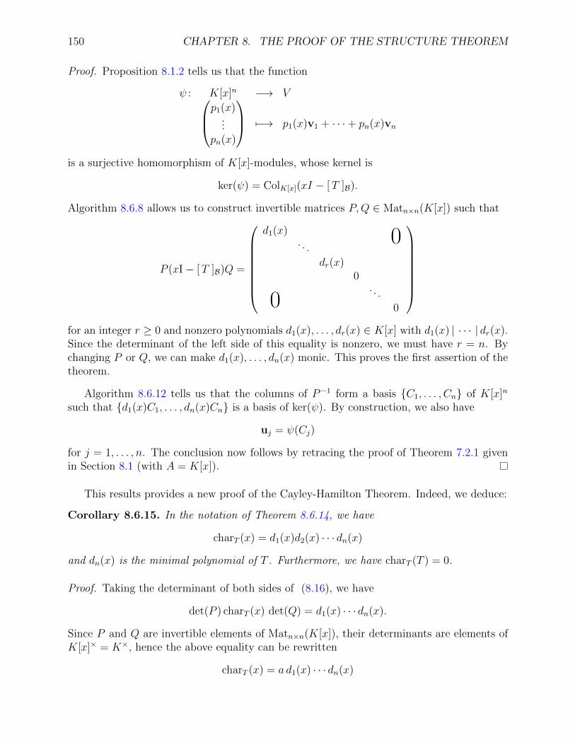
150 CHAPTER 8. THE PROOF OF THE STRUCTURE THEOREM
Proof. Proposition 8.1.2 tells us that the function
ψ : K[x]n −→ Vp1(x)...
pn(x)
7−→ p1(x)v1 + · · ·+ pn(x)vn
is a surjective homomorphism of K[x]-modules, whose kernel is
ker(ψ) = ColK[x](xI − [T ]B).
Algorithm 8.6.8 allows us to construct invertible matrices P,Q ∈ Matn×n(K[x]) such that
P (xI− [T ]B)Q =
d1(x) 0. . .
dr(x)0
0. . .
0
for an integer r ≥ 0 and nonzero polynomials d1(x), . . . , dr(x) ∈ K[x] with d1(x) | · · · | dr(x).Since the determinant of the left side of this equality is nonzero, we must have r = n. Bychanging P or Q, we can make d1(x), . . . , dn(x) monic. This proves the first assertion of thetheorem.
Algorithm 8.6.12 tells us that the columns of P−1 form a basis {C1, . . . , Cn} of K[x]n
such that {d1(x)C1, . . . , dn(x)Cn} is a basis of ker(ψ). By construction, we also have
uj = ψ(Cj)
for j = 1, . . . , n. The conclusion now follows by retracing the proof of Theorem 7.2.1 givenin Section 8.1 (with A = K[x]).
This results provides a new proof of the Cayley-Hamilton Theorem. Indeed, we deduce:
Corollary 8.6.15. In the notation of Theorem 8.6.14, we have
charT (x) = d1(x)d2(x) · · · dn(x)
and dn(x) is the minimal polynomial of T . Furthermore, we have charT (T ) = 0.
Proof. Taking the determinant of both sides of (8.16), we have
det(P ) charT (x) det(Q) = d1(x) · · · dn(x).
Since P and Q are invertible elements of Matn×n(K[x]), their determinants are elements ofK[x]× = K×, hence the above equality can be rewritten
charT (x) = a d1(x) · · · dn(x)

8.6. ALGORITHMS 151
for some constant a ∈ K×. Since the polynomials charT (x) and d1(x), . . . , dn(x) are bothmonic, we must have a = 1. Now, Theorem 7.2.4 tells us that dn(x) is the minimal polynomialof T . We deduce that
charT (T ) = d1(T ) ◦ · · · ◦ dn(T ) = 0.
Applying Theorem 7.2.5, we also obtain:
Corollary 8.6.16. With the notation of Theorem 8.6.14, let mi = deg(di(x)) for i =k, . . . , n. Then
C ={uk, T (uk), . . . , T
mk−1(uk), . . . . . . , un, T (un), . . . , Tmn−1(un)}
is a basis of V such that
[T ]C =
Dk 00
. . .
Dn
where Di denotes the companion matrix of di(x) for i = k, . . . , n.
Example 8.6.17. Let V be a vector space over Q of dimension 3, let B = {v1,v2,v3} be abasis of V , and let T : V → V be a linear operator for which
[T ]B =
0 −1 −1−3 2 34 −4 −5
.
Find a basis C of V such that [T ]C is in rational canonical form.
Solution: We first apply Algorithm 8.6.8 to the matrix
U = xI − [T ]B =
x 1 13 x− 2 −3−4 4 x+ 5
.
Since we only need the matrix P , we work with the table (U | I). Retracing the calculationsof Example 8.5.7, we find
(U | I) ∼
C2 C1 1 x 1 1 0 0x− 2 3 −3 0 1 0
4 −4 x+ 5 0 0 1
∼
C2 − xC1 C3 − C1 1 0 0 1 0 0x− 2 −x2 + 2x+ 3 −x− 1 0 1 0
4 −4x− 4 x+ 1 0 0 1

152 CHAPTER 8. THE PROOF OF THE STRUCTURE THEOREM
∼
1 0 0 1 0 00 −x2 + 2x+ 3 −x− 1 −x+ 2 1 0 R2 − (x− 2)R1
0 −4x− 4 x+ 1 −4 0 1 R3 − 4R1
∼
C3 C2 1 0 0 1 0 00 −x− 1 −x2 + 2x+ 3 −x+ 2 1 0
0 x+ 1 −4x− 4 −4 0 1
∼
1 0 0 1 0 00 x+ 1 x2 − 2x− 3 x− 2 −1 0 −R2
0 0 −x2 − 2x− 1 −x− 2 1 1 R3 +R2
∼
C3 − (x− 3)C2 1 0 0 1 0 00 x+ 1 0 x− 2 −1 0
0 0 −(x+ 1)2 −x− 2 1 1
∼
1 0 0 1 0 00 x+ 1 0 x− 2 −1 0
0 0 (x+ 1)2 x+ 2 −1 −1 −R3
Thus the invariant factors are 1, x+ 1 and (x+ 1)2. We see that
P−1 =
1 0 0x− 2 −1 0x+ 2 −1 −1
−1
=
1 0 0x− 2 −1 0
4 1 −1
(the verification of this calculation is left as an exercise). We deduce that
V = Q[x]u2 ⊕Q[x]u3 where u2 = −v2 + v3 and u3 = −v3.
Furthermore, the annihilator u2 is generated by x+1 and that of u3 is generated by (x+1)2 =x2 + 2x+ 1. We conclude that
C = {u2,u3, T (u3)} = {−v2 + v3, −v3, v1 − 3v2 + 5v3}
is a basis of V such that
[T ]C =
−1 0 00 0 −10 1 −2
where, on the diagonal, we recognize the companion matrices of x+ 1 and x2 + 2x+ 1.
Note. The first column of P−1 gives
u1 = 1v1 + (x− 1)v2 + 4v3 = v1 + T (v2)− 2v2 + 4v3 = 0
as it should, since the annihilator of u1 is generated by d1(x) = 1.

8.6. ALGORITHMS 153
Exercises.
In all the exercises below, A denotes a euclidean domain.
8.6.1. Prove Lemma 8.6.2.
8.6.2. Let P ∈ Matn×n(A).
(i) Give an algorithm for transforming P into an upper triangular matrix T by a series ofelementary row operations.
(ii) Show that P is invertible if and only if the diagonal element of T are units of A.
(iii) If the diagonal elements of T are units, give an algorithm for transforming T into Inby a series of elementary row operations.
(iv) Conclude that, if P is invertible, then P can be transformed into the matrix In by aseries of elementary row operations.
Hint. For part (i), show that P is invertible if and only if T is invertible and use the factthat a matrix in Matn×n(A) is invertible if and only if its determinant is a unit of A (seeAppendix B).
8.6.3. Problem 8.6.2 shows that, in the statement of Theorem 8.6.10, the condition (i) impliescondition (ii). Complete the proof of this theorem by proving the implications (ii) ⇒ (iii)and (iii) ⇒ (i), and then proving the last assertion of the theorem.
8.6.4. For each of the matrix U of Exercise 8.5.2, find invertible matrices P and Q such thatPUQ is in Smith normal form.
8.6.5. In each case below, find a basis {C1, . . . , Cn} of An and nonzero elements d1, . . . , drof A with d1 | d2 | · · · | dr such that {d1C1, . . . , drCr} is a basis of the given submodule N ofAn.
(i) A = Q[x], N =
⟨ xx+ 1x
,
0xx2
⟩Q[x]
(ii) A = R[x], N =
⟨x+ 1−1−2
,
−4x+ 1
4
,
4−2x− 5
⟩R[x]
(iii) A = Z, N =
⟨(48
),
(410
),
(28
)⟩Z

154 CHAPTER 8. THE PROOF OF THE STRUCTURE THEOREM
(iv) A = Z, N =
⟨ 4120
,
084
,
48−2
⟩Z
8.6.6. Let V be a finite-dimensional vector space over a field K, and let T : V → V be alinear map. Show that minT (x) and charT (x) have the same irreducible factors in K[x].
Hint. Use Corollary 8.6.15.
8.6.7. Let T : Q3 → Q3 be a linear map. Suppose that charT (x) admits an irreducible factorof degree ≥ 2 in Q[x]. Show that Q3 is a cyclic Q[x]-module.
8.6.8. Let V be a vector space of dimension 2 over Q with basis B = {v1,v2}, and let
T : V → V be a linear map with [T ]B =
(3 1−1 1
).
(i) Find charT (x) and minT (x).
(ii) Find a basis C of V such that [T ]C is block diagonal with companion matrices ofpolynomials on the diagonal.
8.6.9. Let A =
4 2 21 3 1−3 −3 −1
∈ Mat3×3(Q).
(i) Find charA(x) and minA(x).
(ii) Find a matrix D that is similar to A and that is block diagonal with companion matricesof polynomials on the diagonal.

Chapter 9
Duality and the tensor product
In this chapter, we present some linear algebraic constructions that play an important rolein numerous areas of mathematics, as much in analysis as in algebra.
9.1 Duality
Definition 9.1.1. Let V be a vector space over a field K. The dual of V is the vector spaceLK(V,K) of linear maps from V to K. We denote it by V ∗. An element of V ∗ is called alinear form on V .
Example 9.1.2. Let X be a set and let F(X,K) be the vector space of functions g : X → K.For all x ∈ X, the function
Ex : F(X,K) −→ Kg 7−→ g(x)
called evaluation at the point x, is linear, thus Ex ∈ F(X,K)∗.
Proposition 9.1.3. Suppose that V is finite dimensional over K and that B = {v1, . . . ,vn}is a basis of V . For each i = 1, . . . , n, we denote by fi : V → K the linear map such that
fi(vj) = δij :=
{0 if j 6= i,
1 if j = i.
Then B∗ = {f1, . . . , fn} is a basis of V ∗.
We say that B∗ is the basis of V ∗ dual to B.
Proof. We know that E = {1} is a basis of K viewed as a vector space over itself. ThenTheorem 2.4.3 gives us an isomorphism
LK(V,K)∼−→ Mat1×n(K) .
f 7−→ [ f ]BE
155

156 CHAPTER 9. DUALITY AND THE TENSOR PRODUCT
For i = 1, . . . , n, we see that
[ fi ]BE =
([fi(v1)]E · · · [fi(vn)]E
)= (0, . . . ,
i∨1, . . . , 0) = eti.
Since {et1, . . . , etn} is a basis of Mat1×n(K), we deduce that {f1, . . . , fn} is a basis of V ∗.
Proposition 9.1.4. Let V and W be vector spaces over K and let T : V → W be a linearmap. For each linear form g : W → K, the composition g ◦ T : V → K is a linear form onV . Furthermore, the function
tT : W ∗ −→ V ∗
g 7−→ g ◦ T
is linear.
We say that tT is the transpose of T .
Proof. The first assertion follows from the fact that the composition of two linear maps islinear. The fact that tT is linear follows from Proposition 2.3.1.
Example 9.1.5. Let X and Y be two sets, and let h : X → Y be a function. One can verifythat the map
T : F(Y,K) −→ F(X,K)g 7−→ g ◦ h
is linear (exercise). In this context, we determine tT (Ex) where Ex ∈ F(X,K)∗ denotes theevaluation at a point x of X (see Example 9.1.2).
For all g ∈ F(Y,K), we have
(tT (Ex))(g) = (Ex ◦ T )(g) = Ex(T (g)) = Ex(g ◦ h) = (g ◦ h)(x) = g(h(x)) = Eh(x)(g),
hence tT (Ex) = Eh(x).
Proposition 9.1.6. Let U , V and W be vector spaces over K.
(i) If S, T ∈ LK(V,W ) and c ∈ K, then
t(S + T ) = tS + tT and t(cT ) = c tT .
(ii) If S ∈ LK(U, V ) and T ∈ LK(V,W ), then
t(T ◦ S) = tS ◦ tT .
The proof of this result is left as an exercise. Part (i) implies:

9.1. DUALITY 157
Corollary 9.1.7. Let V and W be vector spaces over K. The function
LK(V,W ) −→ LK(W ∗, V ∗)T 7−→ tT
is linear.
Theorem 9.1.8. Let V and W be finite-dimensional vector spaces over K, let
B = {v1, . . . ,vn} and D = {w1, . . . ,wm}
be bases, respectively, of V and W , and let
B∗ = {f1, . . . , fn} and D∗ = {g1, . . . , gm}
be the bases of V ∗ and W ∗ dual, respectively, to B and D. For all T ∈ LK(V,W ), we have
[ tT ]D∗
B∗ =([T ]BD
)t.
In other words, the matrix of the transpose tT of T relative to the dual bases D∗ and B∗is the transpose of the matrix of T relative to the bases B and D.
Proof. Let T ∈ LK(V,W ). Write [T ]BD = (aij). By definition, we have
T (vj) = a1jw1 + · · ·+ amjwm (j = 1, . . . , n).
We know that tT ∈ LK(W ∗, V ∗) and we want to find
[ tT ]D∗
B∗ =(
[tT (g1)]B∗ · · · [tT (gm)]B∗).
Fix an index j ∈ {1, . . . ,m}. For all i = 1, . . . , n, we have
(tT (gj))(vi) = (gj ◦ T )(vi) = gj(T (vi)) = gj
( m∑k=1
akiwk
)= aji.
We deduce that
tT (gj) =n∑i=1
ajifi
(see Exercise 9.1.1). Thus, [tT (gj)]B∗ is the transpose of the row j of [T ]BD. This gives
[ tT ]D∗
B∗ =
a11 · · · am1...
...a1n · · · amn
=([T ]BD
)t

158 CHAPTER 9. DUALITY AND THE TENSOR PRODUCT
Definition 9.1.9 (Double dual). The double dual of a vector space V is the dual of V ∗. Wedenote it V ∗∗.
We thus have V ∗∗ = LK(V ∗, K). The following result is particularly important.
Theorem 9.1.10. Let V be a vector space over K.
(i) For all v ∈ V , the function
Ev : V ∗ −→ Kf 7−→ f(v)
is linear and so Ev ∈ V ∗∗.
(ii) The functionϕ : V −→ V ∗∗
v 7−→ Ev
is also linear.
(iii) If V is finite-dimensional, then ϕ is an isomorphism.
Proof. (i) Let v ∈ V . For all f, g ∈ V ∗ and c ∈ K, we have
Ev(f + g) = (f + g)(v) = f(v) + g(v) = Ev(f) + Ev(g) ,
Ev(c f) = (c f)(v) = c f(v) = cEv(f) .
(ii) Let u,v ∈ V and c ∈ K. For all f ∈ V ∗, we have
Eu+v(f) = f(u + v) = f(u) + f(v) = Eu(f) + Ev(f) = (Eu + Ev)(f) ,
Ecv(f) = f(cv) = c f(v) = cEv(f) = (cEv)(f) ,
hence Eu+v = Eu + Ev and Ecv = cEv. This shows that ϕ is linear.
(iii) Suppose that V is finite-dimensional. Let B = {v1, . . . ,vn} be a basis of V and letB∗ = {f1, . . . , fn} be the basis of V ∗ dual to B. We have
Evj(fi) = fi(vj) = δij (1 ≤ i, j ≤ n).
Thus {Ev1 , . . . , Evn} is the basis of (V ∗)∗ = V ∗∗ dual to B∗. Since ϕ maps B to this basis,the linear map ϕ is an isomorphism.
It can be shown that the map ϕ defined in Theorem 9.1.10 is always injective (even if Vis infinite-dimensional). It is an isomorphism if and only if V is finite-dimensional.

9.1. DUALITY 159
Exercises.
9.1.1. Let V be a finite-dimensional vector space over a field K, let B = {v1, . . . ,vn} be abasis of V , and let B∗ = {f1, . . . , fn} be the basis of V ∗ dual to B. Show that, for all f ∈ V ∗,we have
f = f(v1)f1 + · · ·+ f(vn)fn.
9.1.2. Prove Proposition 9.1.6.
9.1.3. Consider the vectors v1 = (1, 0, 1)t, v2 = (0, 1,−2)t and v3 = (−1,−1, 0)t of R3.
(i) If f is a linear form on R3 such that
f(v1) = 1, f(v2) = −1, f(v3) = 3,
and if v = (a, b, c)t, determine f(v).
(ii) Give an explicit linear form f on R3 such that f(v1) = f(v2) = 0 but f(v3) 6= 0.
(iii) Let f be a linear form on R3 such that f(v1) = f(v2) = 0 and f(v3) 6= 0. Show that,for v = (2, 3,−1)t, we have f(v) 6= 0.
9.1.4. Consider the vectors v1 = (1, 0,−i)t, v2 = (1, 1, 1)t and v3 = (i, i, 0)t of C3. Showthat B = {v1,v2,v3} is a basis of C3 and determine the basis B∗ of (C3)∗ dual to B.
9.1.5. Let V = 〈 1, x, x2 〉R be the vector space of polynomial functions p : R → R of degreeat most 2. We define three linear forms f1, f2, f3 on V by setting
f1(p) =
∫ 1
0
p(x)dx, f2(p) =
∫ 2
0
p(x)dx, f3(p) =
∫ 0
−1
p(x)dx.
Show that B = {f1, f2, f3} is a basis of V ∗ and find its dual basis in V .
9.1.6. Let m and n be positive integers, let K be a field, and let f1, . . . , fm be linear formson Kn.
(i) Verify that the function T : Kn → Km given by
T (v) =
f1(v)...
fm(v)
for all v ∈ Kn,
is a linear map.

160 CHAPTER 9. DUALITY AND THE TENSOR PRODUCT
(ii) Show that every linear map from Kn to Km can be written in this way for some choiceof f1, . . . , fm ∈ (Kn)∗.
9.1.7. Let n be a positive integer and let K be a field. Set V = Matn×n(K). Recallthat the trace of a matrix A = (ai,j) ∈ V is the sum of the elements of its diagonal:trace(A) =
∑ni=1 ai,i.
(i) Verify that the function trace : V → K is a linear form on V .
(ii) Let B ∈ V . Show that the map ϕB : V → K given by ϕB(A) = trace(AB) for allA ∈ V is linear.
(iii) Show that the function Φ: V → V ∗ given by Φ(B) = ϕB for all B ∈ V is linear.
(iv) Show that ker Φ = {0} and conclude that Φ is an isomorphism.
9.2 Bilinear maps
Let U , V and W be vector spaces over a field K.
Definition 9.2.1 (Bilinear map, bilinear form). A bilinear map from U×V to W is a functionB : U × V → W that satisfies
(i) B(u,v1 + v2) = B(u,v1) +B(u,v2),
(ii) B(u1 + u2,v) = B(u1,v) +B(u2,v),
(iii) B(cu,v) = B(u, cv) = cB(u,v)
for every choice of u,u1,u2 ∈ U , of v,v1,v2 ∈ V and of c ∈ K. A bilinear form on U × V isa bilinear map from U × V to K.
Therefore, a bilinear map from U × V to W is a function B : U × V → W such that,
1) for all u ∈ U , the function V → W is linear;v 7→ B(u,v)
2) for all v ∈ V , the function U → W is linear.u 7→ B(u,v)
We express condition 1) by saying that B is right linear and condition 2) by saying that Bis left linear .
Example 9.2.2. The function
B : V × V ∗ −→ K(v, f) 7−→ f(v)
is a bilinear form on V × V ∗ since, for every choice of v,v1,v2 ∈ V , of f, f1, f2 ∈ V ∗ and ofc ∈ K, we have

9.2. BILINEAR MAPS 161
(i) (f1 + f2)(v) = f1(v) + f2(v),
(ii) f(v1 + v2) = f(v1) + f(v2),
(iii) f(cv) = c f(v) = (c f)(v).
Example 9.2.3. Proposition 2.3.1 shows that the function
LK(U, V )× LK(V,W ) −→ LK(U,W )(S, T ) 7−→ T ◦ S
is a bilinear map.
Definition 9.2.4. We denote by L2K(U, V ;W ) the set of bilinear maps from U × V to W .
The following result provides an analogue of Theorem 2.2.3 for bilinear maps.
Theorem 9.2.5. For all B1, B2 ∈ L2K(U, V ;W ) and c ∈ K, the functions
B1 +B2 : U × V −→ W and cB1 : U × V −→ W(u,v) 7−→ B1(u,v) +B2(u,v) (u,v) 7−→ cB1(u,v)
are bilinear. The set L2K(U, V ;W ) equipped with the addition and scalar multiplication defined
above is a vector space over K.
The proof of the first assertion is similar to that of Proposition 2.2.1 while the secondassertion can be proved by following the model of the proof of Theorem 2.2.3. These proofsare left as exercises.
In Exercise 9.2.3, an outline is given of a proof that we have a natural isomorphism:
L2K(U, V ;W )
∼−→ LK(U,LK(V,W )
)B 7−→ (u 7→ (v 7→ (B(u,v)))
We conclude this section with the following results:
Theorem 9.2.6. Suppose that U and V admit bases
A = {u1, . . . ,um} and B = {v1, . . . ,vn}
respectively. Then, for all wij ∈ W (1 ≤ i ≤ m, 1 ≤ j ≤ n), there exists a unique bilinearmap B : U × V → W satisfying
B(ui,vj) = wij (1 ≤ i ≤ m, 1 ≤ j ≤ n). (9.1)

162 CHAPTER 9. DUALITY AND THE TENSOR PRODUCT
Proof. Let wij ∈ W (1 ≤ i ≤ m, 1 ≤ j ≤ n).
1st Uniqueness. If there is a bilinear map B : U × V → W satisfying (9.1), then
B
(m∑i=1
aiui,n∑j=1
bjvj
)=
m∑i=1
aiB
(ui,
n∑j=1
bjvj
)
=m∑i=1
ai
(n∑j=1
bjB(ui,vj)
)
=m∑i=1
n∑j=1
aibjwij
for all a1, . . . , am, b1, . . . , bn ∈ K. This proves that there exists at most one such bilinearmap.
2nd Existence. Consider the function B : U × V → W defined by
B
(m∑i=1
aiui,n∑j=1
bjvj
)=
m∑i=1
n∑j=1
aibjwij.
It satisfies conditions (9.1). It remains to prove that it is bilinear. We have
B
(m∑i=1
aiui,n∑j=1
bjvj +n∑j=1
b′jvj
)= B
(m∑i=1
aiui,n∑j=1
(bj + b′j)vj
)
=m∑i=1
n∑j=1
ai(bj + b′j)wij
=m∑i=1
n∑j=1
aibjwij +m∑i=1
n∑j=1
aib′jwij
= B
(m∑i=1
aiui,n∑j=1
bjvj
)+B
(m∑i=1
aiui,n∑j=1
b′jvj
),
for all a1, . . . , am, b1, . . . , bn, b′1, . . . , b
′n ∈ K. We also verify that
B
(m∑i=1
aiui, cn∑j=1
bjvj
)= cB
(m∑i=1
aiui,n∑j=1
bjvj
),
for all c ∈ K. Thus B is right linear. We check similarly that B is left linear. Therefore, Bis bilinear.
Theorem 9.2.7. Suppose that U and V admit bases
A = {u1, . . . ,um} and B = {v1, . . . ,vn}

9.2. BILINEAR MAPS 163
respectively. Let B : U × V → K be a bilinear form on U × V . Then there exists a uniquematrix M ∈ Matm×n(K) such that
B(u,v) = [u]tAM [v]B (9.2)
for all u ∈ U and all v ∈ V . The element in row i and column j of M is B(ui,vj).
The matrix M is called the matrix of the bilinear form B relative to the bases A of Uand B of V .
Proof. 1st Existence. Let u ∈ U and v ∈ V . They can be written in the form
u =m∑i=1
aiui and v =n∑j=1
bjvj
with a1, . . . , am, b1, . . . , bn ∈ K. We have
B(u,v) =m∑i=1
n∑j=1
aibjB(ui,vj)
= (a1, . . . , am)
B(u1,v1) · · · B(u1,vn)...
...B(um,v1) · · · B(um,vn)
b1
...bn
= [u]tA
(B(ui,vj)
)[v]B .
2nd Uniqueness. Suppose that M ∈ Matm×n(K) satisfies condition (9.2) for all u ∈ U andall v ∈ V . For i = 1, . . . ,m and j = 1, . . . , n, we have
B(ui,vj) = [ui]tAM [vj]B = (0, . . . ,
i∨1, . . . , 0)M
0...1...0
← j
= element in (i, j) position of M .
Example 9.2.8. Suppose that B = {v1, . . . ,vn} is a basis of V . Let B∗ = {f1, . . . , fn} be thedual basis of V ∗. We calculate the matrix of the bilinear form
B : V × V ∗ −→ K(v, f) 7−→ f(v)
relative to these bases.
Solution: We have B(vi, fj) = fj(vi) = δij for 1 ≤ i, j ≤ n, hence the matrix of B is(δij) = In, the n× n identity matrix.

164 CHAPTER 9. DUALITY AND THE TENSOR PRODUCT
Exercises.
9.2.1. Let V and W be vector spaces over a field K and let v ∈ V . Show that the map
B : V ∗ ×W −→ W(f,w) 7−→ f(v)w
is bilinear.
9.2.2. Let T , U , V and W be vector spaces over a field K, let B : U × V → T be a bilinearmap and let L : T → W be a linear map. Show that the composite
L ◦B : U × V −→ W
is a bilinear map.
9.2.3. Let U, V,W be vector spaces over a field K. For all B ∈ L2K(U, V ;W ) and all u ∈ U ,
we denote by Bu : V → W the linear map given by
Bu(v) = B(u,v) (v ∈ V ).
(i) Let B ∈ L2K(U, V ;W ). Show that the map
ϕB : U −→ LK(V ;W )u 7−→ Bu
is linear.
(ii) Show that the map
ϕ : L2K(U, V ;W ) −→ LK(U,LK(V ;W ))
B 7−→ ϕB
is an isomorphism of vector spaces over K.
9.2.4. Let {e1, e2} be the standard basis of R2 and {e′1, e′2, e′3} be the standard basis of R3.Give a formula for f((x1, x2, x3), (y1, y2)) where f : R3 × R2 → R denotes the bilinear mapdetermined by the conditions
f(e′1, e1) = 1, f(e′1, e2) = 0, f(e′2, e1) = 3,f(e′2, e2) = −1, f(e′3, e1) = 4, f(e′3, e2) = −2.
Deduce the value of f(u,v) if u = (1, 2, 1)t and v = (1, 0)t.

9.2. BILINEAR MAPS 165
9.2.5. Let U , V and W be vector spaces over a field K, let Bi : U × V → W (i = 1, 2) bebilinear maps, and let c ∈ K. Show that the maps
B1 +B2 : U × V −→ W and cB1 : U × V −→ W(u,v) 7−→ B1(u,v) +B2(u,v) (u,v) 7−→ cB1(u,v)
are bilinear. Then show that L2K(U, V ; W ) is a vector space for these operations (since this
verification is a bit long, you can simply show the existence of an additive identity, that everyelement has an additive inverse and that one of the two axioms of distributivity holds).
9.2.6. Let V be a vector space of finite dimension n over a field K, and let B = {v1, . . . ,vn}be a basis of V . For every pair of integers i, j ∈ {1, . . . , n}, we denote by gi,j : V × V → Kthe bilinear form determined by the conditions
gi,j(vk,v`) =
{1 if (k, `) = (i, j),
0 otherwise.
Show that B = { gi,j ; 1 ≤ i, j ≤ n } is a basis of the vector space Bil(V,K) := L2K(V, V ; K)
of all bilinear maps from V × V to K.
9.2.7. Let V be a vector space over a field K of characteristic different from 2. We say thata bilinear form f : V × V → K is symmetric if f(u,v) = f(v,u) for all u ∈ V and v ∈ V .We say that it is antisymmetric if f(u,v) = −f(v,u) for all u ∈ V and v ∈ V .
(i) Show that the set S of symmetric bilinear forms on V ×V is a subspace of Bil(V,K) :=L2K(V, V ; K).
(ii) Show that the set A of antisymmetric bilinear forms on V × V is also a subspace ofBil(V,K).
(iii) Show that Bil(V,K) = S ⊕ A.
9.2.8. Find a basis of the space of symmetric bilinear forms from R2 × R2 to R and a basisof the space of antisymmetric bilinear forms from R2 × R2 to R.
9.2.9. Let C(R) be the vector space of continuous functions from R to R, and let V be thesubspace of C(R) generated (over R) by the functions 1, sin(x) and cos(x). Show that thefunction
B : V × V −→ R(f, g) 7−→
∫ π0f(t)g(π − t)dt
is a bilinear form and find its matrix with respect to the basis A = {1, sin(x), cos(x)} of V .
9.2.10. Let V = 〈 1, x, . . . , xn 〉R be the vector space of polynomial functions p : R → R ofdegree at most n. Find the matrix of the bilinear map
B : V × V −→ R(f, g) 7−→
∫ 1
0f(t)g(t)dt
with respect to the basis A = {1, x, . . . , xn} of V .

166 CHAPTER 9. DUALITY AND THE TENSOR PRODUCT
9.3 Tensor product
Throughout this section, we fix two vector spaces U and V of finite dimension over a fieldK.
If T is a vector space, we can consider a bilinear map from U × V to T as a product
U × V −→ T(u,v) 7−→ u⊗ v
(9.3)
with values in T . To say that this map is bilinear means that the product in questionsatisfies:
(u1 + u2)⊗ v = u1 ⊗ v + u2 ⊗ v,
u⊗ (v1 + v2) = u⊗ v1 + u⊗ v2,
(cu)⊗ v = u⊗ (cv) = cu⊗ v,
for all u,u1,u2 ∈ U , all v,v1,v2 ∈ V and all c ∈ K.
Given a bilinear map as above in (9.3), we easily check that, for every linear map L : T →W , the composite B : U × V → W given by
B(u,v) = L(u⊗ v) for all (u,v) ∈ U × V (9.4)
is a bilinear map (see Exercise 9.2.2).
Our goal is to construct a bilinear map (9.3) that is universal in the sense that everybilinear map B : U × V → W can be written in the form (9.4) for a unique choice of linearmap L : T → W . A bilinear map (9.3) with this property is called a tensor product of U andV . The following definition summarizes this discussion.
Definition 9.3.1 (Tensor product). A tensor product of U and V is the data of a vector spaceT over K and a bilinear map
U × V −→ T(u,v) 7−→ u⊗ v
possessing the following property. For every vector space W and every bilinear map B : U ×V → W , there exists a unique linear map L : T → W such that B(u,v) = L(u⊗ v) for all(u,v) ∈ U × V .
This condition can be represented by the following diagram:
U × V
⊗↓T ·········
B→ W
L(9.5)

9.3. TENSOR PRODUCT 167
In this diagram, the vertical arrow represents the tensor product, the horizontal arrow repre-sents an arbitrary bilinear map, and the dotted diagonal arrow represents the unique linearmap L that, by composition with the tensor product, recovers B. For such a choice of L,the horizontal arrow B is the composition of the two other arrows and we say that thediagram (9.5) is commutative.
The following proposition gives the existence of a tensor product of U and V .
Proposition 9.3.2. Let {u1, . . . ,um} be a basis of U , let {v1, . . . ,vn} be a basis of V , andlet {tij ; 1 ≤ i ≤ m, 1 ≤ j ≤ n} be a basis of a vector space T of dimension mn over K. Thebilinear map (9.3) determined by the conditions
ui ⊗ vj = tij (1 ≤ i ≤ m, 1 ≤ j ≤ n) (9.6)
is a tensor product of U and V .
Proof. Theorem 9.2.6 shows that there exists a bilinear map (u,v) 7−→ u ⊗ v from U × Vto T satisfying 9.6. It remains to show that it satisfies the universal property required byDefinition 9.3.1.
To do this, we fix an arbitrary bilinear map B : U × V → W . Since the set {tij ; 1 ≤ i ≤m, 1 ≤ j ≤ n} is a basis of T , there exists a unique linear map L : T → W such that
L(tij) = B(ui,vj) (1 ≤ i ≤ m, 1 ≤ j ≤ n). (9.7)
Then the map B′ : U × V → W given by B′(u,v) = L(u ⊗ v) for all (u,v) ∈ U × V isbilinear and satisfies
B′(ui,vj) = L(ui ⊗ vj) = L(tij) = B(ui,vj) (1 ≤ i ≤ m, 1 ≤ j ≤ n).
By Theorem 9.2.6, this implies that B′ = B. Thus the map L satisfies the condition
B(u,v) = L(u⊗ v) for all (u,v) ∈ U × V .
Finally, L is the only linear map from T to W satisfying this condition since the latterimplies (9.7), which determines L uniquely.
The proof given above uses in a crucial way the hypotheses that U and V are finite-dimensional over K. It is possible to prove the existence of the tensor product in greatergenerality, without this hypothesis, but we will not do so here.
We next observe that the tensor product is unique up to isomorphism.
Proposition 9.3.3. Suppose that
U × V −→ T and U × V −→ T ′
(u,v) 7−→ u⊗ v (u,v) 7−→ u⊗′ v
are two tensor products of U and V . Then there exists an isomorphism L : T → T ′ such that
L(u⊗ v) = u⊗′ v
for all (u,v) ∈ U × V .

168 CHAPTER 9. DUALITY AND THE TENSOR PRODUCT
Proof. Since ⊗′ is bilinear and ⊗ is a tensor product, there exists a linear map L : T → T ′
such thatu⊗′ v = L(u⊗ v) (9.8)
for all (u,v) ∈ U × V . It remains to prove that L is an isomorphism. For this, we first notethat, symmetrically, since ⊗ is bilinear and ⊗′ is a tensor product, there exists a linear mapL′ : T ′ → T such that
u⊗ v = L′(u⊗′ v) (9.9)
for all (u,v) ∈ U × V . Combining (9.8) and (9.9), we obtain
(L′ ◦ L)(u⊗ v) = u⊗ v and (L ◦ L′)(u⊗′ v) = u⊗′ v
for all (u,v) ∈ U × V . Now, the identity maps I : T → T and I ′ : T ′ → T ′ also satisfy
I(u⊗ v) = u⊗ v and I ′(u⊗′ v) = u⊗′ v
for all (u,v) ∈ U × V . Since ⊗ and ⊗′ are tensor products, this implies that L′ ◦L = I andL◦L′ = I ′. Thus L is an invertible linear map with inverse L′, and so it is an isomorphism.
Combining Proposition 9.3.2 and 9.3.3, we obtain the following.
Proposition 9.3.4. Let {u1, . . . ,um} be a basis of U , let {v1, . . . ,vn} be a basis of V , andlet ⊗ : U × V → T be a tensor product of U and V . Then
{ui ⊗ vj ; 1 ≤ i ≤ m, 1 ≤ j ≤ n} (9.10)
is a basis of T .
Proof. Proposition 9.3.2 shows that there exists a tensor product ⊗ : U × V → T suchthat (9.10) is a basis of T . If ⊗′ : U × V → T ′ is another tensor product, then, by Propo-sition 9.3.3, there exists an isomorphism L : T → T ′ such that u ⊗′ v = L(u ⊗ v) for all(u,v) ∈ U × V . Since (9.10) is a basis of T , we deduce that the products
ui ⊗′ vj = L(ui ⊗ vj) (1 ≤ i ≤ m, 1 ≤ j ≤ n)
form a basis of T ′.
The following theorem summarizes the essential results obtained up to now:
Theorem 9.3.5. There exists a tensor product ⊗ : U ×V → T of U and V . If {u1, . . . ,um}is a basis of U and {v1, . . . ,vn} is a basis of V , then {ui ⊗ vj ; 1 ≤ i ≤ m, 1 ≤ j ≤ n} is abasis of T .
We often say that T itself is the tensor product of U and V and we denote it by U⊗V or,more precisely, by U ⊗K V when we want to emphasize the fact that U and V are consideredas vector spaces over K. Theorem 9.3.5 gives
dimK(U ⊗K V ) = dimK(U) dimK(V ).

9.3. TENSOR PRODUCT 169
The fact that the tensor product is not unique, but is unique up to isomorphism, doesnot cause problems in practice, in the sense that the linear dependence relations betweenthe products u⊗ v with u ∈ U and v ∈ V do not depend on the tensor product ⊗. In factif, for a given tensor product ⊗ : U × V → T , we have:
c1u1 ⊗ v1 + c2u2 ⊗ v2 + · · ·+ csus ⊗ vs = 0 (9.11)
with c1, . . . , cs ∈ K, u1, . . . ,us ∈ U and v1, . . . ,vs ∈ V , and if ⊗′ : U × V → T ′ is anothertensor product, then, denoting by L : T → T ′ the isomorphism such that L(u⊗ v) = u⊗′ vfor all (u,v) ∈ U × V and applying L to both sides of (9.11), we get
c1u1 ⊗′ v1 + c2u2 ⊗′ v2 + · · ·+ csus ⊗′ vs = 0.
Example 9.3.6. Let {e1, e2} be the standard basis of K2. A basis of K2 ⊗K K2 is
{e1 ⊗ e1, e1 ⊗ e2, e2 ⊗ e1, e2 ⊗ e2}.
In particular, we have e1 ⊗ e2 − e2 ⊗ e1 6= 0, hence e1 ⊗ e2 6= e2 ⊗ e1. We also find
(e1 + e2)⊗ (e1 − e2) = e1 ⊗ (e1 − e2) + e2 ⊗ (e1 − e2)
= e1 ⊗ e1 − e1 ⊗ e2 + e2 ⊗ e1 − e2 ⊗ e2.
More generally, we have
(a1e1 + a2e2)⊗ (b1e1 + b2e2) =( 2∑i=1
aiei
)⊗( 2∑j=1
bjej
)=
2∑i=1
2∑j=1
aibjei ⊗ ej
= a1b1e1 ⊗ e1 + a1b2e1 ⊗ e2 + a2b1e2 ⊗ e1 + a2b2e2 ⊗ e2.
Example 9.3.7. We know that the scalar product in Rn is a bilinear form
Rn × Rn −→ R .(u,v) 7−→ 〈u,v〉
Thus these exists a unique linear map L : Rn ⊗R Rn → R such that
〈u,v〉 = L(u⊗ v)
for all u,v ∈ Rn. Let {e1, . . . , en} be the standard basis of Rn. Then the set {ei ⊗ ej ; 1 ≤i ≤ n, 1 ≤ j ≤ n} is a basis of Rn ⊗R Rn and so L is determined by the conditions
L(ei ⊗ ej) = 〈ei, ej〉 = δij (1 ≤ i ≤ n, 1 ≤ j ≤ n).

170 CHAPTER 9. DUALITY AND THE TENSOR PRODUCT
Exercises.
9.3.1. Let {e1, e2} be the standard basis of R2. Show that e1⊗e2 +e2⊗e1 cannot be writtenin the form u⊗ v with u,v ∈ R2.
9.3.2. Let {e1, e2} be the standard basis of R2, let B : R2 × R2 → R2 be the bilinear mapdetermined by the conditions
B(e1, e1) = (1, 0), B(e1, e2) = (2, 1), B(e2, e1) = (−1, 3) and B(e2, e2) = (0,−1),
and let L : R2⊗RR2 → R2 be the linear map such that B(u,v) = L(u⊗v) for all u,v ∈ R2.Calculate
(i) L(e1 ⊗ e2 − e2 ⊗ e1),
(ii) L((e1 + 2e2)⊗ (−e1 + e2)),
(iii) L(e1 ⊗ e1 + (e1 + e2)⊗ e2).
9.3.3. Let V be a finite-dimensional vector space over a field K. Show that there exists aunique linear form L : V ∗⊗K V → K satisfying the condition L(f ⊗v) = f(v) for all f ∈ V ∗and v ∈ V .
9.3.4. Let U and V be finite-dimensional vector spaces over a field K and let {u1, . . . ,um}be a basis of U . Show that every element t of U ⊗K V can be written in the form
t = u1 ⊗ v1 + u2 ⊗ v2 + · · ·+ um ⊗ vm
for a unique choice of vectors v1,v2, . . . ,vm ∈ V .
9.3.5. Let U , V be finite-dimensional vector spaces over a field K.
(i) Let U1 and V1 be subspaces of U and V respectively and let T1 be the subspace ofU ⊗K V generated by the products u⊗ v with u ∈ U1 and v ∈ V1. Show that the map
U1 × V1 −→ T1
(u,v) 7−→ u⊗ v
is a tensor product of U1 and V1. We can then identify T1 with U1 ⊗K V1.
(ii) Suppose that U = U1 ⊕ U2 and V = V1 ⊕ V2. Show that
U ⊗K V = (U1 ⊗K V1)⊕ (U2 ⊗K V1)⊕ (U1 ⊗K V2)⊕ (U2 ⊗K V2).
9.3. TENSOR PRODUCT 171
9.3.6. Let V be a finite-dimensional vector space over R. Considering C as a vector spaceover R, we form the tensor product C⊗R V .
(i) Show that, for all α ∈ C, there exists a unique linear map Lα : C ⊗R V → C ⊗R Vsatisfying Lα(β ⊗ v) = (αβ)⊗ v for all β ∈ C and v ∈ V .
(ii) Show that, for all α, α′ ∈ C, we have Lα ◦ Lα′ = Lαα′ and Lα + Lα′ = Lα+α′ . Deducethat C⊗RV is a vector space over C for the external multiplication given by αt = Lα(t)for all α ∈ C and v ∈ V .
(iii) Show that if {v1, . . . ,vn} is a basis of V as a vector space over R, then {1⊗v1, . . . , 1⊗vn} is a basis of C⊗R V as a vector space over C.
We say that C⊗R V is the complexification of V .
9.3.7. With the notation of the preceding problem, show that every element t of C⊗R V canbe written in the form t = 1 ⊗ u + i ⊗ v for unique u,v ∈ V , and also that every complexnumber α ∈ C can be written in the form α = a+ ib for unique a, b ∈ R. Given α and u asabove, determine the decomposition of the product αt.
9.3.8. Let V and W be finite-dimensional vector spaces over a field K.
(i) Show that, for all f ∈ V ∗ and w ∈ W , the map
Lf,w : V −→ Wv 7−→ f(v)w
is linear.
(ii) Show also that the mapV ∗ ×W −→ LK(V,W )
(f,w) 7−→ Lf,w
is bilinear.
(iii) Deduce that there exists a unique isomorphism L : V ∗ ⊗K W∼−→ LK(V,W ) satisfying
L(f ⊗w) = Lf,w for all f ∈ V ∗ and w ∈ W .
9.3.9. With the notation of the proceeding problem, let B = {v1, . . . ,vn} be a basis of V ,let {f1, . . . , fn} be the basis of V ∗ dual to B, and let D = {w1, . . . ,wm} be a basis of W .Fix T ∈ LK(V,W ) and set [T ]BD = (aij). Show that, under the isomorphism L of part (iii)of the preceding problem, we have
T = L
(m∑i=1
n∑j=1
aijfj ⊗wi
).

172 CHAPTER 9. DUALITY AND THE TENSOR PRODUCT
9.3.10. Let K be a field of characteristic not equal to 2, and let V be a vector space over Kof dimension n with basis A = {v1, . . . ,vn}. For every pair of elements u, v of V , we define
u ∧ v :=1
2(u⊗ v − v ⊗ u) and u · v :=
1
2(u⊗ v + v ⊗ u).
Let∧2 V be the subspace of V ⊗K V generated by the vectors u ∧ v, and let Sym2(V ) be
the subspace generated by the vectors u · v.
(i) Show that the set B1 = {vi ∧ vj ; 1 ≤ i < j ≤ n} is a basis of∧2 V while B2 =
{vi ·vj ; 1 ≤ i ≤ j ≤ n} is a basis of Sym2(V ). Deduce that V ⊗KV =∧2 V ⊕Sym2(V ).
(ii) Show that the map ϕ1 : V × V →∧2 V given by ϕ1(u,v) = u ∧ v is antisymmetric
bilinear and that the map ϕ2 : V ×V → Sym2(V ) given by ϕ2(u,v) = u·v is symmetricbilinear (see Exercise 9.2.7 for the definitions).
(iii) Let B : V × V → W be an arbitrary antisymmetric bilinear map. Show that thereexists a unique linear map L1 :
∧2 V → W such that B = L1 ◦ ϕ1.
(iv) State and prove the analogue of (iii) for a symmetric bilinear map.
Hint. For (iii), let L : V ⊗ V → W be the linear map satisfying B(u,v) = L(u ⊗ v) for allu,v ∈ V . Show that Sym2(V ) ⊆ ker(L) and that B(u,v) = L(u ∧ v) for all u,v ∈ V .
9.4 The Kronecker product
In this section, we fix finite-dimensional vector spaces U and V over a field K and we fix atensor product
U × V −→ U ⊗K V .(u,v) 7−→ u⊗ v
We first note:
Proposition 9.4.1. Let S ∈ EndK(U) and T ∈ EndK(V ). Then there exists a uniqueelement of EndK(U ⊗K V ), denoted S ⊗ T , such that
(S ⊗ T )(u⊗ v) = S(u)⊗ T (v)
for all (u,v) ∈ U × V .
Proof. The map
B : U × V −→ U ⊗K V(u,v) 7−→ S(u)⊗ T (v)

9.4. THE KRONECKER PRODUCT 173
is left linear since
B(u1 + u2,v) = S(u2 + u2)⊗ T (v) and B(cu,v) = S(cu)⊗ T (v)
= (S(u1) + S(u2))⊗ T (v) = (c S(u))⊗ T (v)
= S(u1)⊗ T (v) + S(u2)⊗ T (v) = c (S(u)⊗ T (v))
= B(u1,v) +B(u2,v) = cB(u,v)
for all u,u1,u2 ∈ U , v ∈ V and c ∈ K. Similarly, we verify that B is right linear. Thus itis a bilinear map. By the properties of the tensor product, we conclude that there exists aunique linear map L : U ⊗K V → U ⊗K V such that
L(u⊗ v) = S(u)⊗ T (v)
for all u ∈ U and v ∈ V .
The tensor product of the operators defined by Proposition 9.4.1 possesses a number ofproperties (see the exercises). We show here the following:
Proposition 9.4.2. Let S1, S2 ∈ EndK(U) and T1, T2 ∈ EndK(V ). Then we have
(S1 ⊗ T1) ◦ (S2 ⊗ T2) = (S1 ◦ S2)⊗ (T1 ◦ T2).
Proof. For all (u,v) ∈ U × V , we have
((S1 ⊗ T1) ◦ (S2 ⊗ T2))(u⊗ v) = (S1 ⊗ T1)((S2 ⊗ T2)(u⊗ v))
= (S1 ⊗ T1)(S2(u)⊗ T2(v))
= S1(S2(u))⊗ T1(T2(v))
= (S1 ◦ S2)(u)⊗ (T1 ◦ T2)(v).
By Proposition 9.4.1, this implies that (S1 ⊗ T1) ◦ (S2 ⊗ T2) = (S1 ◦ S2)⊗ (T1 ◦ T2).
Definition 9.4.3 (Kronecker product). The Kronecker product of a matrix A = (aij) ∈Matm×m(K) by a matrix B = (bij) ∈ Matn×n(K) is the matrix
A×B =
a11B a12B · · · a1mBa21B a22B · · · a2mB
......
...am1B am2B · · · ammB
∈ Matmn×mn(K).
Our interest in this notion comes from the following result:
Proposition 9.4.4. Let S ∈ EndK(U) and T ∈ EndK(V ), and let
A = {u1, . . . ,um} and B = {v1, . . . ,vn}
be bases of U and V respectively. Then
C = {u1 ⊗ v1, . . . ,u1 ⊗ vn; u2 ⊗ v1, . . . ,u2 ⊗ vn; . . . . . . ; um ⊗ v1, . . . ,um ⊗ vn}
is a basis of U ⊗K V and we have
[S ⊗ T ]C = [S ]A×[T ]B.

174 CHAPTER 9. DUALITY AND THE TENSOR PRODUCT
Proof. The matrix [S ⊗ T ]C decomposes naturally in blocks:︷ ︸︸ ︷u1 ⊗ v1, . . . ,u1 ⊗ vn · · ·
︷ ︸︸ ︷um ⊗ v1, . . . ,um ⊗ vn
u1 ⊗ v1
... C11 · · · C1m
u1 ⊗ vn...
......
um ⊗ v1... Cm1 · · · Cmm
um ⊗ vn
.
For fixed k, l ∈ {1, . . . ,m}, the block Ckl is the following piece:
· · · ul ⊗ v1, . . . ,ul ⊗ vn · · ·...
uk ⊗ v1
... Ckluk ⊗ vn
...
.
The (i, j) element of Ckl is thus equal to the coefficient of uk ⊗ vi in the expression of(S ⊗ T )(ul ⊗ vj) as a linear combination of elements of the basis C. To calculate it, write
A = [S ]A =
a11 · · · a1m...
...am1 · · · amm
and B = [T ]B =
b11 · · · b1n...
...bn1 · · · bnn
.
We see that
(S ⊗ T )(ul ⊗ vj) = S(ul)⊗ T (vj)
= (a1lu1 + · · ·+ amlum)⊗ (b1jv1 + · · ·+ bnjvn)
= · · · + (aklb1juk ⊗ v1 + · · ·+ aklbnjuk ⊗ vn) + · · ·
hence the (i, j) entry of Ckl is aklbij, equal to that of aklB. This proves that Ckl = aklB andso
[S ⊗ T ]C = A×B = [S ]A×[T ]B.

9.4. THE KRONECKER PRODUCT 175
Exercises.
9.4.1. Denote by E = {e1, e2} the standard basis of R2 and by E ′ = {e′1, e′2, e′3} that of R3.Let S : R2 → R2 and T : R3 → R3 be the linear operators for which
[S ]E =
(1 2−1 0
)and [T ]E ′ =
1 1 00 1 11 0 1
.
Calculate
(i) (S ⊗ T )(3e1 ⊗ e′1),
(ii) (S ⊗ T )(2e1 ⊗ e′1 − e2 ⊗ e′2),
(iii) (S ⊗ T )(2(e1 + e2)⊗ e′3 − e2 ⊗ e′3).
9.4.2. Let U and V be finite-dimensional vector spaces over a field K, and let S : U → U andT : V → V be invertible linear maps. Show that the linear map S ⊗ T : U ⊗K V → U ⊗K Vis also invertible, and give an equation relating S−1, T−1 and (S ⊗ T )−1.
9.4.3. Let S ∈ EndK(U) and T ∈ EndK(V ), where U and V denote finite-dimensional vectorspaces over a field K. Let U1 be an S-invariant subspace of U and let V1 be a T -invariantsubspace of V . Consider U1 ⊗K V1 as a subspace of U ⊗K V as in Exercise 9.3.5. Underthese hypotheses, show that U1 ⊗K V1 is an S ⊗ T -invariant subspace of U ⊗K V and that(S ⊗ T )|U1⊗KV1
= S|U1⊗ T |V1 .
9.4.4. Let S ∈ EndC(U) and T ∈ EndC(V ), where U and V denote vector spaces of dimen-sions m and n respectively over C. We choose a basis A of U and a basis B of V such thatthe matrix [S ]A and [T ]B are in Jordan canonical form. Show that, for the correspondingbasis C of U ⊗C V given by Proposition 9.4.4, the matrix [S ⊗ T ]C is upper triangular. Bycalculating its determinant, show that det(S ⊗ T ) = det(S)n det(T )m.
9.4.5. Let U and V be finite-dimensional vector spaces over a field K.
(i) Show that the map
B : EndK(U)× EndK(V ) −→ EndK(U ⊗K V )(S, T ) 7−→ S ⊗ T
is bilinear.
(ii) Show that the image of B generates EndK(U ⊗K V ) as a vector space over K.

176 CHAPTER 9. DUALITY AND THE TENSOR PRODUCT
(iii) Conclude that the linear map from EndK(U)⊗KEndK(V ) to EndK(U⊗KV ) associatedto B is an isomorphism.
9.4.6. Let U and V be finite-dimensional vector spaces over a field K.
(i) Let f ∈ U∗ and g ∈ V ∗. Show that there exists a unique linear form f⊗g : U⊗KV → Ksuch that (f ⊗ g)(u⊗ v) = f(u)g(v) for all (u,v) ∈ U × V .
(ii) Show that the map B : U∗ × V ∗ → (U ⊗K V )∗ given by B(f, g) = f ⊗ g for all(f, g) ∈ U∗ × V ∗ is bilinear and that its image generates (U ⊗K V )∗ as a vector spaceover K. Conclude that the linear map from U∗ ⊗K V ∗ to (U ⊗K V )∗ associated to Vis an isomorphism.
(iii) Let S ∈ EndK(U) and T ∈ EndK(V ). Show that, if we identify U∗ ⊗K V ∗ with(U ⊗K V )∗ using the isomorphism established in (ii), then we have tS⊗ tT = t(S ⊗ T ).
9.5 Multiple tensor products
Theorem 9.5.1. Let U, V,W be finite-dimensional vector spaces over a field K. There existsa unique isomorphism L : (U ⊗K V )⊗K W → U ⊗K (V ⊗K W ) such that
L((u⊗ v)⊗w) = u⊗ (v ⊗w)
for all (u,v,w) ∈ U × V ×W .
Proof. Let {u1, . . . ,ul}, {v1, . . . ,vm} and {w1, . . . ,wn} be bases of U , V and W respectively.Then
{(ui ⊗ vj)⊗wk ; 1 ≤ i ≤ l, 1 ≤ j ≤ m, 1 ≤ k ≤ n},{ui ⊗ (vj ⊗wk) ; 1 ≤ i ≤ l, 1 ≤ j ≤ m, 1 ≤ k ≤ n}
are bases, respectively, of (U ⊗K V )⊗KW and U ⊗K (V ⊗KW ). Thus there exists a uniquelinear map L from (U ⊗K V )⊗K W to U ⊗K (V ⊗K W ) such that
L((ui ⊗ vj)⊗wk) = ui ⊗ (vj ⊗wk)
for i = 1, . . . , l, j = 1, . . . ,m and k = 1, . . . , n. By construction, L is an isomorphism.Finally, for arbitrary vectors
u =l∑
i=1
aiui ∈ U, v =m∑j=1
bjvj ∈ V and w =n∑k=1
ckwk ∈ W,

9.5. MULTIPLE TENSOR PRODUCTS 177
we have
L((u⊗ v)⊗w) = L
(((l∑
i=1
aiui
)⊗
(m∑j=1
bjvj
))⊗
(n∑k=1
ckwk
))
= L
(l∑
i=1
m∑j=1
n∑k=1
aibjck(ui ⊗ vj)⊗wk
)
=l∑
i=1
m∑j=1
n∑k=1
aibjck ui ⊗ (vj ⊗wk)
=
(l∑
i=1
aiui
)⊗
((m∑j=1
bjvj
)⊗
(n∑k=1
ckwk
))= u⊗ (v ⊗w),
as required.
The isomorphism (U ⊗K V )⊗K W ' U ⊗K (V ⊗K W ) given by Theorem 9.5.1 allows usto identify these two spaces, and to denote them by U⊗K V ⊗KW . We then write u⊗v⊗winstead of (u⊗ v)⊗w or u⊗ (v ⊗w).
In general, Theorem 9.5.1 allows us to omit the parentheses in the tensor product of anarbitrary number of finite-dimensional vector spaces V1, . . . , Vr over K. Thus, we write
V1 ⊗K V2 ⊗K · · · ⊗K Vr instead of V1 ⊗K (V2 ⊗K (· · · ⊗K Vr))
andv1 ⊗ v2 ⊗ · · · ⊗ vr instead of v1 ⊗ (v2 × (· · · ⊗ vr)).
We then have
dimK(V1 ⊗K V2 ⊗K · · · ⊗K Vr) = dimK(V1) dimK(V2) · · · dimK(Vr).
Exercises.
9.5.1. Let V and W be finite-dimensional vector space over a field K. Show that there existsa unique isomorphism L : V ⊗K W → W ⊗K V such that L(v ⊗w) = w ⊗ v for all v ∈ Vand w ∈ W .
9.5.2. Let r be a positive integer and V1, . . . , Vr,W be vector spaces over K. We say that afunction
ϕ : V1 × · · · × Vr −→ W
is multilinear or r-linear if it is linear in each of its arguments, that is if it satisfies

178 CHAPTER 9. DUALITY AND THE TENSOR PRODUCT
ML1. ϕ(v1, . . . ,vi + v′i, . . . ,vr) = ϕ(v1, . . . ,vi, . . . ,vr) + ϕ(v1, . . . ,v′i, . . . ,vr)
ML2. ϕ(v1, . . . , cvi, . . . ,vr) = c ϕ(v1, . . . ,vi, . . . ,vr)
for all i ∈ {1, . . . , r},v1 ∈ V1, . . . ,vi,v′i ∈ Vi, . . . ,vr ∈ Vr and c ∈ K.
Show that the function
ψ : V1 × V2 × · · · × Vr −→ V1 ⊗K V2 ⊗K · · · ⊗K Vr(v1,v2, . . . ,vr) 7−→ v1 ⊗ v2 ⊗ · · · ⊗ vr
is multilinear.
9.5.3. Let V1, . . . , Vr and W be as in the preceding exercise. The goal of this new exerciseis to show that, for any multilinear map ϕ : V1 × · · · × Vr → W , there exists a unique linearmap L : V1 ⊗K · · · ⊗K Vr → W such that
ϕ(v1, . . . ,vr) = L(v1 ⊗ v2 ⊗ · · · ⊗ vr)
for all (v1, . . . ,vr) ∈ V1 × · · · × Vr.
We proceed by induction on r. For r = 2, this follows from the definition of the tensorproduct. Suppose r ≥ 3 and the result is true for multilinear maps from V2× · · · × Vr to W .
(i) Show that, for each choice of v1 ∈ V1, there exists a unique linear map Lv1 : V2 ⊗K· · · ⊗K Vr → W such that
ϕ(v1,v2, . . . ,vr) = Lv1(v2 ⊗ · · · ⊗ vr)
for all (v2, . . . ,vr) ∈ V2 × · · · × Vr.
(ii) Show that the map
B : V1 × (V2 ⊗K · · · ⊗K Vr) −→ W(v1, α) 7−→ Lv1(α)
is bilinear.
(iii) Deduce that there exists a unique linear map L : V1 ⊗K (V2 ⊗K · · · ⊗K Vr) → W suchthat ϕ(v1, . . . ,vr) = L(v1 ⊗ (v2 ⊗ · · · ⊗ vr)) for all (v1, . . . ,vr) ∈ V1 × · · · × Vr.
9.5.4. Let V be a finite-dimensional vector space over a field K. Using the result of thepreceding exercise, show that there exists a unique linear map L : V ∗⊗K V ⊗K V → V suchthat L(f ⊗ v1 ⊗ v2) = f(v1)v2 for all (f,v1,v2) ∈ V ∗ × V × V .
9.5.5. Let V1, V2, V3 and W be finite-dimensional vector spaces over a field K, and letϕ : V1 × V2 × V3 → W be a trilinear map. Show that there exists a unique bilinear mapB : V1× (V2⊗K V3)→ W such that B(v1,v2⊗v3) = ϕ(v1,v2,v3) for all vj ∈ Vj (j = 1, 2, 3).

Chapter 10
Inner product spaces
After a general review of inner product spaces, we define the notions of orthogonal operatorsand symmetric operators on these spaces and prove the structure theorems for these operators(the spectral theorems). We conclude by showing that every linear operator on a finite-dimensional inner product space is the composition of a positive definite symmetric operatorfollowed by an orthogonal operator. This decomposition is called the polar decompositionof an operator. For example, in R2, a positive definite symmetric operator is a product ofdilations along orthogonal axes, while an orthogonal operator is a rotation about the originor a reflection in a line passing through the origin. Therefore every linear operator on R2 isthe composition of dilations along orthogonal axes follwed by a rotation or reflection.
10.1 Review
Definition 10.1.1 (Inner product). Let V be a real vector space. An inner product on V isa bilinear form
V × V −→ R(u,v) 7−→ 〈u,v〉
that is symmetric:〈u,v〉 = 〈v,u〉 for all u,v ∈ V
and positive definite:
〈v,v〉 ≥ 0 for all v ∈ V , with 〈v,v〉 = 0 ⇐⇒ v = 0 .
Definition 10.1.2 (Inner product space). A inner product space is a real vector space Vequipped with an inner product.
Example 10.1.3. Let n be a positive integer. We define an inner product on Rn by setting⟨x1...xn
,
y1...yn
⟩ = x1y1 + · · ·+ xnyn.
179

180 CHAPTER 10. INNER PRODUCT SPACES
Equipped with this inner product, Rn becomes an inner product space, called euclidean space.When we speak of Rn as an inner product space without specifying the inner product, weare implicitly using the inner product defined above.
Example 10.1.4. Let V be the vector space of continuous functions f : R → R that are 2π-periodic, that is, which satisfy f(x + 2π) = f(x) for all x ∈ R. Then V is an inner productspace for the inner product
〈f, g〉 =
∫ 2π
0
f(x)g(x)dx .
Example 10.1.5. Let n be a positive integer. Then Matn×n(R) is an inner product space forthe inner product 〈A,B〉 = trace(ABt).
For the rest of this section, we fix an inner product space V with inner product 〈 , 〉. Wefirst note:
Proposition 10.1.6. Every subspace W of V is an inner product space for the inner productof V restricted to W .
Proof. Indeed, the inner product of V induces, by restriction, a bilinear map
W ×W −→ R(w1,w2) 7−→ 〈w1,w2〉
and it is easily verified that this is an inner product in the sense of Definition 10.1.1.
When we refer to a subspace of V as an inner product space, it is this inner product weare referring to.
Definition 10.1.7 (Norm, unit vector). The norm of a vector v ∈ V is
‖v‖ = 〈v,v〉1/2.
We say that a vector v ∈ V is a unit vector if ‖v‖ = 1.
Recall that the norm possesses the following properties, the first two of which followimmediately from the definition:
Proposition 10.1.8. For all u,v ∈ V and c ∈ R, we have
(i) ‖v‖ ≥ 0 with equality if and only if v = 0,
(ii) ‖cv‖ = |c| ‖v‖,
(iii) |〈u,v〉| ≤ ‖u‖‖v‖ (Cauchy-Schwarz inequality),
(iv) ‖u + v‖ ≤ ‖u‖+ ‖v‖ (triangle inequality).

10.1. REVIEW 181
Relations (i), (ii) and (iv) show that ‖·‖ is indeed a norm in the proper sense of the term.The norm allows us to measure the “length” of vectors in V . It also allows us to define the“distance” d(u,v) between two vectors u and v of V by setting
d(u,v) = ‖u− v‖.
Thanks to the triangle inequality, it is easily verified that this defines a metric on V .
Inequality (iii), called the Cauchy-Schwarz inequality, allows us to define the angle θ ∈[0, π] between two nonzero vectors u and v of V by setting
θ = arccos
(〈u,v〉‖u‖‖v‖
). (10.1)
In particular, this angle θ is equal to π/2 if and only if 〈u,v〉 = 0. For this reason, we saythat the vectors u,v of V are perpendicular or orthogonal if 〈u,v〉 = 0.
Finally, if v ∈ V is nonzero, it follows from (ii) that the product
‖v‖−1v
is a unit vector parallel to v (the angle between it and v is 0 radians by (10.1)).
Definition 10.1.9. Let v1, . . . ,vn ∈ V.
1) We say that {v1, . . . ,vn} is an orthogonal subset of V if vi 6= 0 for i = 1, . . . , n and if〈vi,vj〉 = 0 for every pair of integers (i, j) with 1 ≤ i, j ≤ n and i 6= j.
2) We say that {v1, . . . ,vn} is an orthogonal basis of V , if is it both a basis of V and anorthogonal subset of V .
3) We say that {v1, . . . ,vn} is an orthonormal basis of V if it is an orthogonal basis of Vconsisting of unit vectors, that is, such that ‖vi‖ = 〈vi,vi〉1/2 = 1 for i = 1, . . . , n.
The following proposition summarizes the importance of these ideas.
Proposition 10.1.10.
(i) Every orthogonal subset of V is linearly independent.
(ii) Suppose that B = {v1, . . . ,vn} is an orthogonal basis of V . Then, for all v ∈ V , wehave
v =〈v,v1〉〈v1,v1〉
v1 + · · ·+ 〈v,vn〉〈vn,vn〉
vn.
(iii) If B = {v1, . . . ,vn} is an orthonormal basis of V , then, for all v ∈ V , we have
[v]B =
〈v,v1〉...
〈v,vn〉
.

182 CHAPTER 10. INNER PRODUCT SPACES
Proof. Suppose first that {v1, . . . ,vn} is an orthogonal subset of V , and that v ∈ 〈v1, . . . ,vn〉R.We can write
v = a1v1 + · · ·+ anvn
with a1, . . . , an ∈ R. Taking the inner product of both sides of this equality with vi, we have
〈v,vi〉 =⟨ n∑j=1
ajvj,vi
⟩=
n∑j=1
aj〈vj,vi〉 = ai〈vi,vi〉
and so
ai =〈v,vi〉〈vi,vi〉
(i = 1, . . . , n).
If we choose v = 0, this formula gives a1 = · · · = an = 0. Thus the set {v1, . . . ,vn} islinearly independent and thus it is a basis of 〈v1, . . . ,vn〉R. This proves both (i) and (ii).Statement (iii) follows immediately from (ii).
The following result shows that, if V is finite-dimensional, it possesses an orthogonalbasis. In particular, this holds for every finite-dimensional subspace of V .
Theorem 10.1.11 (Gram-Schimdt orthogonalization procedure).Suppose that {w1, . . . ,wn} is a basis of V . We recursively define:
v1 = w1,
v2 = w2 −〈w2,v1〉〈v1,v1〉
v1,
v3 = w3 −〈w3,v1〉〈v1,v1〉
v1 −〈w3,v2〉〈v2,v2〉
v2,
...
vn = wn −〈wn,v1〉〈v1,v1〉
v1 − · · · −〈wn,vn−1〉〈vn−1,vn−1〉
vn−1.
Then, for all i = 1, . . . , n, the set {v1, . . . ,vi} is an orthogonal basis of the subspace 〈w1, . . . ,wi〉R.In particular, {v1, . . . ,vn} is an orthogonal basis of V .
Proof. It suffices to show the first assertion. For this, we proceed by induction on i. Fori = 1, it is clear that {v1} is an orthogonal basis of 〈w1〉R since v1 = w1 6= 0. Suppose that{v1, . . . ,vi−1} is an orthogonal basis of 〈w1, . . . ,wi−1〉R for an integer i with 2 ≤ i ≤ n. Bydefinition, we have
vi = wi −〈wi,v1〉〈v1,v1〉
v1 − · · · −〈wi,vi−1〉〈vi−1,vi−1〉
vi−1, (10.2)
and we note that the denominators 〈v1,v1〉, . . . , 〈vi−1,vi−1〉 of the coefficients of v1, . . . ,vi−1
are nonzero since each of the vectors v1, . . . ,vi−1 is nonzero. We deduce from this formulathat
〈v1, . . . ,vi−1,vi〉R = 〈v1, . . . ,vi−1,wi〉R = 〈w1, . . . ,wi−1,wi〉R.

10.1. REVIEW 183
Then, to conclude that {v1, . . . ,vi} is an orthogonal basis of 〈w1, . . . ,wi〉R, it remains toshow that this is an orthogonal set (by Proposition 10.1.10). For this, it suffices to showthat 〈vi,vj〉 = 0 for j = 1, . . . , i− 1. By (10.2), we see that
〈vi,vj〉 = 〈wi,vj〉 −i−1∑k=1
〈wi,vk〉〈vk,vk〉
〈vk,vj〉 = 0
for j = 1, . . . , i− 1. This completes the proof.
We end this section with a review of the notion of orthogonal complement and two relatedresults.
Definition 10.1.12 (Orthogonal complement). The orthogonal complement of a subspace Wof V is
W⊥ := {v ∈ V ; 〈v,w〉 = 0 for all w ∈ W}.
Proposition 10.1.13. Let W be a subspace of V . Then W⊥ is a subspace of V that satisfiesW ∩W⊥ = {0}. Furthermore, if W = 〈w1, . . . ,wm〉R, then
W⊥ = {v ∈ V ; 〈v,wi〉 = 0 for i = 1, . . . ,m}.
Proof. We leave it as an exercise to show that W⊥ is a subspace of V . We note that, ifw ∈ W ∩W⊥, then we have 〈w,w〉 = 0 and so w = 0. This shows that W ∩W⊥ = {0}.Finally, if W = 〈w1, . . . ,wm〉, we see that
v ∈ W⊥ ⇐⇒ 〈v, a1w1 + · · ·+ amwm〉 = 0 ∀ a1, . . . , am ∈ R⇐⇒ a1〈v,w1〉+ · · ·+ am〈v,wm〉 = 0 ∀ a1, . . . , am ∈ R⇐⇒ 〈v,w1〉 = · · · = 〈v,wm〉 = 0,
and thus the final assertion of the proposition follows.
It follows from Proposition 10.1.13 that V ⊥ = {0}. In other words, for v ∈ V , we have
v = 0 ⇐⇒ 〈u, v〉 = 0 for all u ∈ V.
Theorem 10.1.14. Let W be a finite-dimensional subspace of V . Then we have:
V = W ⊕W⊥.
Proof. Since, by Proposition 10.1.13, we have W ∩ W⊥ = {0}, it remains to show thatV = W +W⊥. Let {w1, . . . ,wm} be an orthogonal basis of W (such a basis exists since Wis finite-dimensional). Given v ∈ V , we set
w =〈v,w1〉〈w1,w1〉
w1 + · · ·+ 〈v,wm〉〈wm,wm〉
wm. (10.3)

184 CHAPTER 10. INNER PRODUCT SPACES
For i = 1, . . . ,m, we see that
〈v −w,wi〉 = 〈v,wi〉 − 〈w,wi〉 = 0,
thus v −w ∈ W⊥, and sov = w + (v −w) ∈ W +W⊥.
Since the choice v ∈ V is arbitrary, this shows that V = W +W⊥, as claimed.
If W is a finite-dimensional subspace of V , Theorem 10.1.14 tells us that, for all v ∈ V ,there exists a unique vector w ∈ W such that v −w ∈ W⊥.
W
v
w
0��
����1
�
··········
We say that this vector w is the orthogonal projection of v on W . If {w1, . . . ,wm} is anorthogonal basis of W , then this projection w is given by (10.3).
Example 10.1.15. Calculate the orthogonal projection of v = (0, 1, 1, 0)t on the subspace Wof R4 generated by w1 = (1, 1, 0, 0)t and w2 = (1, 1, 1, 1)t.
Solution: We first apply the Gram-Schmidt algorithm to the basis {w1,w2} of W . We obtain
v1 = w1 = (1, 1, 0, 0)t
v2 = w2 −〈w2,v1〉〈v1,v1〉
v1 = (1, 1, 1, 1)t − 2
2(1, 1, 0, 0)t = (0, 0, 1, 1)t.
Thus {v1,v2} is an orthogonal basis of W . The orthogonal projection of v on W is therefore
〈v,v1〉〈v1,v1〉
v1 +〈v,v2〉〈v2,v2〉
v2 =1
2v1 +
1
2v2 =
1
2(1, 1, 1, 1)t.
Exercises.
10.1.1. Show that B = {(1,−1, 3)t, (−2, 1, 1)t, (4, 7, 1)t} is an orthogonal basis of R3 andcalculate [(a, b, c)t]B.
10.1.2. Find a, b, c ∈ R such that the set
{(1, 2, 1, 0)t, (1,−1, 1, 3)t, (2,−1, 0,−1)t, (a, b, c, 1)t}
is an orthogonal basis of R4.

10.1. REVIEW 185
10.1.3. Let U and V be inner product spaces equipped with inner products 〈 , 〉U and 〈 , 〉Vrespectively. Show that the formula⟨
(u1,v1), (u2,v2)⟩
= 〈u1,u2〉U + 〈v1,v2〉V
defines an inner product on U × V for which (U × {0})⊥ = {0} × V .
10.1.4. Let V be an inner product space of dimension n equipped with an inner product〈 , 〉.
(i) Verify that, for each u ∈ V , the function fu : V → R given by
fu(v) = 〈u,v〉 for all v ∈ V
belongs to V ∗. Then verify that the map ϕ : V → V ∗ given by ϕ(u) = fu for all u ∈ Vis an isomorphism of vector spaces over R.
(ii) Let B = {u1, . . . ,un} be an orthonormal basis of V . Show that the basis of V ∗ dualto B is B∗ = {f1, . . . , fn}, where fi := ϕ(ui) = fui
for i = 1, . . . , n.
10.1.5. Let V be the vector space of continuous functions f : R→ R that are 2π-periodic.
(i) Show that the formula
〈f, g〉 =
∫ 2π
0
f(x)g(x)dx
defines an inner product on V .
(ii) Show that {1, sin(x), cos(x)} is an orthogonal subset of V for this inner product.
(iii) Let f : R→ R be the periodic “sawtooth” function given on [0, 2π] by
f(x) =
{x if 0 ≤ x ≤ π,
2π − x if π ≤ x ≤ 2π,
and extended by periodicity to all of R. Calculate the projection of f on the subspaceW of V generated by {1, sin(x), cos(x)}.
10.1.6. Let V = Matn×n(R).
(i) Show that the formula 〈A , B〉 = trace(ABt) defines an inner product on V .
(ii) For n = 3, find an orthonormal basis of the subspace S = {A ∈ V ; At = A} ofsymmetric matrices.

186 CHAPTER 10. INNER PRODUCT SPACES
10.1.7. Consider the vector space C[−1, 1] of continuous functions from [−1, 1] to R, equippedwith the inner product
〈f, g〉 =
∫ 1
−1
f(x)g(x) dx .
Find an orthogonal basis of the subspace V = 〈 1, x, x2 〉R.
10.1.8. Let W be the subspace of R4 generated by (1,−1, 0, 1)t and (1, 1, 0, 0)t. Find a basisof W⊥.
10.1.9. Let W1 and W2 be subspaces of a finite-dimensional inner product space V . Showthat W1 ⊆ W2 if and only if W⊥
2 ⊆ W⊥1 .
10.2 Orthogonal operators
In this section, we fix an inner product space V of finite dimension n, and an orthonormalbasis B = {u1, . . . ,un} of V . We first note:
Lemma 10.2.1. For all u,v ∈ V , we have
〈u,v〉 =([u]B
)t[v]B.
Proof. Let u,v ∈ V . Write
u =n∑i=1
aiui and v =n∑i=1
biui
with a1, . . . , an, b1, . . . , bn ∈ R. We have
〈u,v〉 =
⟨n∑i=1
aiui,n∑j=1
bjvj
⟩=
n∑i=1
n∑j=1
aibj〈ui,vj〉 =n∑i=1
aibi
since 〈ui,uj〉 = δij. In matrix form, this equality can be rewritten
〈u,v〉 = (a1, . . . , an)
b1...bn
= [u]tB [v]B.
Using this lemma, we can now show:
Proposition 10.2.2. Let T : V → V be a linear operator. The following conditions areequivalent:

10.2. ORTHOGONAL OPERATORS 187
(i) ‖T (u)‖ = 1 for all u ∈ V with ‖u‖ = 1,
(ii) ‖T (v)‖ = ‖v‖ for all v ∈ V ,
(iii) 〈T (u), T (v)〉 = 〈u,v〉 for all u,v ∈ V ,
(iv) {T (u1), . . . , T (un)} is an orthonormal basis of V ,
(v) [T ]tB [T ]B = In,
(vi) [T ]B is invertible and [T ]−1B = [T ]tB.
Proof. (i)=⇒(ii): Suppose first that T (u) is a unit vector for every unit vector u in V .Let v be an arbitrary vector in V . If v 6= 0, then u := ‖v‖−1v is a unit vector, henceT (u) = ‖v‖−1T (v) is a unit vector and so ‖T (v)‖ = ‖v‖. If v = 0, we have T (v) = 0 andthen the equality ‖T (v)‖ = ‖v‖ is again verified.
(ii)=⇒(iii): Suppose that ‖T (v)‖ = ‖v‖ for all v ∈ V . Let u,v be arbitrary vectors inV . We have
‖u + v‖2 = 〈u + v,u + v〉= 〈u,u〉+ 2〈u,v〉+ 〈v,v〉= ‖u‖2 + 2〈u,v〉+ ‖v‖2.
(10.4)
Applying this formula to T (u) + T (v), we obtain
‖T (u) + T (v)‖2 = ‖T (u)‖2 + 2〈T (u), T (v)〉+ ‖T (v)‖2. (10.5)
Since ‖T (u) + T (v)‖ = ‖T (u + v)‖ = ‖u + v‖, ‖T (u)‖ = ‖u‖ and ‖T (v)‖ = ‖v‖, compar-ing (10.4) and (10.5) gives 〈T (u), T (v)〉 = 〈u,v〉.
(iii)=⇒(iv): Suppose that 〈T (u), T (v)〉 = 〈u,v〉 for all u,v ∈ V . Since {u1, . . . ,un} isan orthonormal basis of V , we deduce that
〈T (ui), T (uj)〉 = 〈ui,uj〉 = δij (1 ≤ i, j ≤ n).
Thus {T (u1), . . . , T (un)} is an orthogonal subset of V consisting of unit vectors. By Propo-sition 10.1.10(i), this set is linearly independent. Since it consists of n vectors and V is ofdimension n, it is a basis of V , hence an orthonormal basis of V .
(iv)=⇒(v): Suppose that {T (u1), . . . , T (un)} is an orthonormal basis of V . Let i, j ∈{1, . . . , n}. By Lemma 10.2.1, we have
δij = 〈T (ui), T (uj)〉 = [T (ui)]tB [T (uj)]B.
Now, [T (ui)]tB is the i-th row of the matrix [T ]tB, and [T (uj)]B is the j-th column of [T ]B.
Thus [T (ui)]tB [T (uj)]B = δij is the entry in row i and column j of [T ]tB [T ]B. Since the
choice of i, j ∈ {1, . . . , n} was arbitrary, this implies that [T ]tB [T ]B = I.
(v)=⇒(vi): Suppose that [T ]tB [T ]B = I. Then [T ]B is invertible with inverse [T ]tB.

188 CHAPTER 10. INNER PRODUCT SPACES
(vi)=⇒(i): Finally, suppose that [T ]B is invertible and that [T ]−1B = [T ]tB. If u is an
arbitrary unit vector in V , we see, by Lemma 10.2.1, that
‖T (u)‖2 = 〈T (u), T (u)〉 = [T (u)]tB [T (u)]B
= ([T ]B[u]B)t ([T ]B[u]B) = [u]tB [T ]tB [T ]B[u]B = [u]tB [u]B = 〈u,u〉 = ‖u‖2 = 1.
Thus T (u) is also a unit vector.
Definition 10.2.3 (Orthogonal operator, orthogonal matrix).
• A linear operator T : V → V satisfying the equivalent conditions of Proposition 10.2.2is called a orthogonal operator or a real unitary operator .
• An invertible matrix A ∈ Matn×n(R) such that A−1 = At is called an orthogonalmatrix .
Condition (i) of Proposition 10.2.2 requires that T sends the set of unit vectors in V toitself. This explains the terminology of a unitary operator.
Condition (iii) of Proposition 10.2.2 means that T preserves the inner product. In par-ticular, this requires that T maps each pair of orthogonal vectors u,v in V to another pairof orthogonal vectors. For this reason, we say that such an operator is orthogonal.
Finally, condition (vi) means:
Corollary 10.2.4. A linear operator T : V → V is orthogonal if and only if its matrixrelative to an orthonormal basis of V is an orthogonal matrix.
Example 10.2.5. The following linear operators are orthogonal:
• a rotation about the origin in R2,
• a reflection in a line passing through the origin in R2,
• a rotation about a line passing through the origin in R3,
• a reflection in a plane passing through the origin in R3.
Definition 10.2.6 (O(V ), On(R)). We denote by O(V ) the set of orthogonal operators on Vand by On(R) the set of orthogonal n× n matrices.
We leave it as an exercise to show that O(V ) is a subgroup of GL(V ) = EndK(V )×, thatOn(R) is a subgroup of GLn(R) = Matn×n(R)×, and that these two groups are isomorphic.

10.2. ORTHOGONAL OPERATORS 189
Example 10.2.7. Let T : R3 → R3 be the linear operator whose matrix relative to the standardbasis E of R3 is
[T ]E =1
3
−1 2 22 −1 22 2 −1
.
Show that T is an orthogonal operator.
Solution: Since E is an orthonormal basis of R3, it suffices to show that [T ]E is an orthogonalmatrix. We have
[T ]tE [T ]E =1
9
−1 2 22 −1 22 2 −1
−1 2 22 −1 22 2 −1
= I,
hence [T ]−1E = [T ]tE , as required.
Exercises.
10.2.1. Let T : V → V be an orthogonal operator. Show that T preserves angles, that is, ifu and v are nonzero vectors in V , the angle between T (u) and T (v) is equal to the anglebetween u and v.
10.2.2. Let T : V → V be an invertible linear operator. Show that the following conditionsare equivalent:
(i) 〈T (u), T (v)〉 = 0 for all u,v ∈ V satisfying 〈u,v〉 = 0.
(ii) T = c S for a (real) unitary operator S : V → V and a real number c 6= 0.
Note. The above shows that we cannot define an orthogonal operator to be a linear operatorthat preserves orthogonality. In this sense, the terminology of a unitary operator is moreappropriate.
10.2.3. Let E be an orthonormal basis of V and let B be an arbitrary basis of V . Show thatthe change of basis matrix P = [ I ]BE is orthogonal if and only if B is also an orthonormalbasis.
10.2.4. Let T : V → V be an orthogonal operator. Suppose that W is a T -invariant subspaceof V . Show that W⊥ is also T -invariant.
10.2.5. Let T : V → V be an orthogonal operator. Show that det(T ) = ±1.

190 CHAPTER 10. INNER PRODUCT SPACES
10.2.6. Let V be an inner product space of dimension n. Show that O(V ) is a subgroup ofGL(V ) = EndK(V )×, that On(R) is a subgroup of GLn(R) = Matn×n(R)×, and define anisomorphism ϕ : O(V )
∼−→ On(R).
10.2.7. Let A ∈ Matn×n(R) be an orthogonal matrix. Show that the columns of A form anorthonormal basis of Rn.
10.2.8. Let V and W be arbitrary inner product spaces. Suppose that there exists a functionT : V → W such that T (0) = 0 and ‖T (v1)− T (v2)‖ = ‖v1 − v2‖ for all v1,v2 ∈ V .
(i) Show that 〈T (v1), T (v2)〉 = 〈v1,v2〉 for all v1,v2 ∈ V .
(ii) Deduce that ‖c1T (v1) + c2T (v2)‖ = ‖c1v1 + c2v2‖ for all v1,v2 ∈ V and c1, c2 ∈ R.
(iii) Conclude that, for all v ∈ V and c ∈ R, we have ‖T (cv) − c T (v)‖ = 0, henceT (cv) = c T (v).
(iv) Using similar reasoning, show that, for all vectors v1,v2 ∈ V , we have ‖T (v1 + v2) −T (v1)− T (v2)‖=0, hence T (v1 + v2) = T (v1) + T (v2).
(v) Conclude that T is a linear map. In particular, show that if V = W is finite-dimensional, then T is an orthogonal operator in the sense of Definition 10.2.3.
A function T : V → W satisfying the conditions given at the beginning of this exercise iscalled an isometry .
Hint. For (i), use formula (10.4) with u = T (v1) and v = −T (v2), then with u = v1 andv = −v2. For (ii), use the same formula with u = c1T (v1) and v = c2T (v2), then withu = c1v1 and v = c2v2.
10.3 The adjoint operator
Using the same notation as in the preceding section, we first show:
Theorem 10.3.1. Let B : V × V → R be a bilinear form on V . There exists a unique pairof linear operators S and T on V such that
B(u,v) = 〈T (u),v〉 = 〈u, S(v)〉 (10.6)
for all u,v ∈ V . Furthermore, let E be an orthonormal basis of V and let M be the matrixof B relative to the basis E. Then we have
[S ]E = M and [T ]E = M t. (10.7)
10.3. THE ADJOINT OPERATOR 191
Proof. 1st Existence. Let S and T be linear operators on V determined by conditions (10.7),and let u,v ∈ V . Since M is the matrix of V in the basis E , we have
B(u,v) = [u]tEM [v]E .
Since [T (u)]E = M t [u]E and [S(v)]E = M [v]E , Lemma 10.2.1 gives
〈T (u),v〉 =(M t [u]E
)t[v]E = [u]tEM [v]E = B(u,v)
and 〈u, S(v)〉 = [u]tE (M [v]E) = B(u,v),
as required.
2nd Uniqueness. Suppose that S ′, T ′ are arbitrary linear operators on V such that
B(u,v) = 〈T ′(u),v〉 = 〈u, S ′(v)〉
for all u,v ∈ V . By subtracting these equalities from (10.6), we get
0 = 〈T ′(u)− T (u),v〉 = 〈u, S ′(v)− S(v)〉
for all u,v ∈ V . We deduce that, for all u ∈ V , we have
T ′(u)− T (u) ∈ V ⊥ = {0},
hence T ′(u) = T (u) and so T ′ = T . Similarly, we see that S ′ = S.
Corollary 10.3.2. For any linear operator T on V , there exists a unique linear operator onV , denoted T ∗, such that
〈T (u),v〉 = 〈u, T ∗(v)〉
for all u,v ∈ V . If E is an orthonormal basis of V , we have [T ∗]E = [T ]tE .
Proof. The function B : V × V → R given by B(u,v) = 〈T (u),v〉 for all (u,v) ∈ V × V isbilinear (exercise). To conclude, it suffices to apply Theorem 10.3.1 to this bilinear form.
Definition 10.3.3 (Adjoint, symmetric, self-adjoint). Let T be a linear operator on V . Theoperator T ∗ : V → V defined by Corollary 10.3.2 is called the adjoint of T . We say that Tis symmetric of self-adjoint if T ∗ = T .
By Corollary 10.3.2, we immediately obtain:
Proposition 10.3.4. Let T : V → V be a linear operator. The following conditions areequivalent:
(i) T is symmetric,
(ii) 〈T (u),v〉 = 〈u, T (v)〉 for all u,v ∈ V ,
(iii) there exists an orthonormal basis E of V such that [T ]E is a symmetric matrix,

192 CHAPTER 10. INNER PRODUCT SPACES
(iv) [T ]E is a symmetric matrix for every orthonormal basis E of V .
The proof of the following properties is left as an exercise.
Proposition 10.3.5. Let S and T be linear operators on V , and let c ∈ R. We have:
(i) (c T )∗ = c T ∗ ,
(ii) (S + T )∗ = S∗ + T ∗ ,
(iii) (S ◦ T )∗ = T ∗ ◦ S∗ ,
(iv) (T ∗)∗ = T .
(v) Furthermore, if T is invertible, then T ∗ is also invertible and (T ∗)−1 = (T−1)∗.
Properties (i) and (ii) imply that the map
EndR(V ) −→ EndR(V )T 7−→ T ∗
is linear. Properties (ii) and (iii) can be summarized by saying that T 7→ T ∗ is a ringanti-homomorphism of EndR(V ). More precisely, because of (iv), we say that it is a ringanti-involution.
Example 10.3.6. Every symmetric matrix A ∈ Matn×n(R) defines a symmetric operator onRn
TA : Rn −→ Rn
X 7−→ AX.
We can verify this directly from the definition by noting that, for all X, Y ∈ Rn, we have
〈TA(X), Y 〉 = (AX)t Y = X tAt Y = X tAY = 〈X,TA(Y )〉.
This also follows from Proposition 10.3.4. Indeed, since the standard basis E of Rn is or-thonormal and [TA ]E = A is a symmetric matrix, the linear operator TA is symmetric.
Example 10.3.7. Let W be a subspace of V , and let P : V → V be the orthogonal projectionon W (that is, the linear map that sends v ∈ V to its orthogonal projection on W ). ThenP is a symmetric operator.
Theorem 10.1.14 shows that V = W ⊕ W⊥. The function P is simply the projectionon the first factor of this sum followed by the inclusion of W into V . Let u,v be arbitraryvectors in V . We have
〈P (u),v〉 = 〈P (u) , (v − P (v)) + P (v)〉 = 〈P (u) , v − P (v)〉+ 〈P (u), P (v)〉.
Since P (u) ∈ W and v − P (v) ∈ W⊥, we have 〈P (u),v − P (v)〉 = 0 and the last equalitycan be rewritten
〈P (u),v〉 = 〈P (u), P (v)〉.A similar calculation gives
〈u, P (v)〉 = 〈P (u), P (v)〉.Thus, we have 〈u, P (v)〉 = 〈P (u),v〉, which shows that P is symmetric.

10.4. SPECTRAL THEOREMS 193
Exercises.
10.3.1. Prove Proposition 10.3.5.
10.3.2. Let T : V → V be a linear operator. Show that ker(T ∗) = (Im(T ))⊥ and thatIm(T ∗) = (ker(T ))⊥.
10.3.3. Let T : V → V be a linear operator. Show that T is an orthogonal operator if andonly if T ∗ ◦ T = I.
10.3.4. We know that V = Matn×n(R) is an inner product space for the inner product〈A,B〉 = trace(ABt) (see Exercise 10.1.6). Fix C ∈ V and consider the linear operatorT : V → V given by T (A) = CA for all A ∈ V . Show that the adjoint T ∗ of T is given byT ∗(A) = CtA for all A ∈ V .
Hint. Use the fact that trace(AB) = trace(BA) for all A,B ∈ V .
10.4 Spectral theorems
We again fix an inner product space V of finite dimension n ≥ 1. We first show that:
Lemma 10.4.1. Let T : V → V be a linear operator on V . There exists a T -invariantsubspace of V of dimension 1 or 2.
Proof. We consider V as an R[x]-module for the product p(x)v = p(T )(v). Let v be anonzero element of V . By Proposition 7.1.7, the annihilator of v is generated by a monicpolynomial p(x) ∈ R[x] of degree ≥ 1. Write p(x) = q(x)a(x) where q(x) is a monicirreducible factor of p(x), and set w = a(x)v. Then the annihilator of w is the ideal ofR[x] generated by q(x). By Proposition 7.1.7, the submodule W := R[x]w is a T -invariantsubspace of V of dimension equal to the degree of q(x). Now, Theorem 5.6.5 shows that allthe irreducible polynomials of R[x] are of degree 1 or 2. Thus W is of dimension 1 or 2.
This lemma suggests the following definition:
Definition 10.4.2 (Minimal invariant subspace, irreducible invariant subspace). Let T : V →V be a linear operator on V . We say that a T -invariant subspace W of V is minimal orirreducible if W 6= {0} and if the only T -invariant subspaces of V contained in W are {0}and W .
It follows from this definition and Lemma 10.4.1 that every nonzero T -invariant subspaceof V contains a minimal T -invariant subspace W , and that such a subspace W is of dimension1 or 2.
For an orthogonal or symmetric operator, we have more:

194 CHAPTER 10. INNER PRODUCT SPACES
Lemma 10.4.3. Let T : V → V be an orthogonal or symmetric linear operator, and let Wbe a T -invariant subspace of V . Then W⊥ is also T -invariant.
Proof. Suppose first that T is orthogonal. Then T |W : W → W is an orthogonal operator onW (it preserves the norm of the elements of W ). Then T |W is invertible and, in particular,surjective. Thus T (W ) = W .
Let v ∈ W⊥. For all w ∈ W , we see that
〈T (v), T (w)〉 = 〈v,w〉 = 0,
thus T (v) ∈ (T (W ))⊥ = W⊥. This shows that W⊥ is T -invariant.
Now suppose that T is symmetric. Let v ∈ W⊥. For all w ∈ W , we have
〈T (v),w〉 = 〈v, T (w)〉 = 0,
since T (w) ∈ W . So we have T (v) ∈ W⊥. Since the choice of v ∈ W⊥ was arbitrary, thisshows that W⊥ is T -invariant.
Lemma 10.4.3 immediately implies:
Proposition 10.4.4. Let T : V → V be an orthogonal or symmetric linear operator. ThenV is a direct sum of minimal T -invariant subspaces
V = W1 ⊕ · · · ⊕Ws
which are pairwise orthogonal, that is, such that Wi ⊆ W⊥j for every pair of distinct integers
i and j with 1 ≤ i, j ≤ s.
To complete our analysis of symmetric or orthogonal linear operators T : V → V , it thussuffices to study the restriction of T to a minimal T -invariant subspace. By Lemma 10.4.1,we know that such a subspace is of dimension 1 or 2. We begin with the case of an orthogonaloperator.
Proposition 10.4.5. Let T : V → V be an orthogonal operator, let W be a minimal T -invariant subspace of V , and let B be an orthonormal basis of W . Then either
dimR(W ) = 1 and [T |W ]B = (±1)
for a choice of sign ±, or
dimR(W ) = 2 and [T |W ]B =
(cos(θ) − sin(θ)sin(θ) cos(θ)
)for some real number θ.

10.4. SPECTRAL THEOREMS 195
Proof. By Lemma 10.4.1, the subspace W is of dimension 1 or 2. Furthermore, the restrictionT |W : W → W of T to W is an orthogonal operator since T |W preserves the norm (seeDefinition 10.2.3). Thus [T |W ]B is an orthogonal matrix, by Corollary 10.2.4.
1st If dimR(W ) = 1, then [T |W ]B = (a) with a ∈ R. Since [T |W ]B is an orthogonal
matrix, we must have (a)t(a) = 1, hence a2 = 1 and so a = ±1.
2nd If dimR(W ) = 2, then the columns of [T |W ]B form an orthonormal basis of R2 (seeExercise 10.2.7), and so this matrix can be written
[T |W ]B =
(cos(θ) −ε sin(θ)sin(θ) ε cos(θ)
)with θ ∈ R and ε = ±1. We deduce that
charT |W
(x) =
∣∣∣∣ x− cos(θ) ε sin(θ)− sin(θ) x− ε cos(θ)
∣∣∣∣ = x2 − (1 + ε) cos(θ)x+ ε.
If ε = −1, the polynomial becomes charT |W
(x) = x2−1 = (x−1)(x+1). Then 1 and −1 are
the eigenvalues of T |W , and for each of these eigenvalues, the operator T |W : W → W has aneigenvector. But if w ∈ W is an eigenvector of T |W then Rw is a T -invariant subspace of Vof dimension 1 contained in W , contradicting the hypothesis that W is a minimal T -invariantsubspace. Therefore, we must have ε = 1 and the proof is complete.
In the case of a symmetric operator, the situation is even simpler.
Proposition 10.4.6. Let T : V → V be a symmetric operator, and let W be a minimalT -invariant subspace of V . Then W is of dimension 1.
Proof. We know that W is of dimension 1 or 2. Suppose that it is of dimension 2, and letB be an orthonormal basis of W . The restriction T |W : W → W is a symmetric operator onW since for all w1,w2 ∈ W , we have
〈T |W (w1),w2〉 = 〈T (w1),w2〉 = 〈w1, T (w2)〉 = 〈w1, T |W (w2)〉.
Thus, by Proposition 10.3.4, the matrix [T |W ]B is symmetric. It can therefore be written inthe form
[T |W ]B =
(a bb c
)with a, b, c ∈ R. We then have
charT |W (x) =
∣∣∣∣ x− a −b−b x− c
∣∣∣∣ = x2 − (a+ c)x+ (ac− b2).
The discriminant of this polynomial is
(a+ c)2 − 4(ac− b2) = (a− c)2 + 4b2 ≥ 0.
Thus charT |W (x) has at least one real root. This root is an eigenvalue of T |W and so itcorresponds to an eigenvector w. Then Rw is a T -invariant subspace of V contained in W ,contradicting the minimality hypothesis on W . Thus W is necessarily of dimension 1.

196 CHAPTER 10. INNER PRODUCT SPACES
Combining the last three propositions, we obtain a description of orthogonal and sym-metric operators on V .
Theorem 10.4.7. Let T : V → V be a linear operator.
(i) If T is orthogonal, there exists an orthonormal basis B of V such that [T ]B is blockdiagonal with blocks of the form
(1), (−1) or
(cos(θ) − sin(θ)sin(θ) cos(θ)
)(10.8)
(with θ ∈ R) on the diagonal.
(ii) If T is symmetric, there exists an orthonormal basis B of V such that [T ]B is a diagonalmatrix.
Result (ii) can be interpreted as saying that a symmetric operator is diagonalizable in anorthonormal basis.
Proof. By Proposition 10.4.4, the space V can be decomposed as a direct sum
V = W1 ⊕ · · · ⊕Ws
of minimal T -invariant subspaces W1, . . . ,Ws which are pairwise orthogonal. Choose anorthonormal basis Bi of Wi for each i = 1, . . . , s. Then
B = B1 q · · · q Bs
is an orthonormal basis of V such that
[T ]B =
[T |W1]B1 0
0. . .
[T |Ws]Bs
.
If T is an orthogonal operator, Proposition 10.4.5 shows that each of the blocks [T |Wi]Bi on
the diagonal is of the form (10.8). On the other hand, if T is symmetric, Proposition 10.4.6shows that each Wi is of dimension 1. Thus, in this case, [T |W ]B is diagonal.
Corollary 10.4.8. Let A ∈ Matn×n(R) be a symmetric matrix. There exists an orthogonalmatrix P ∈ On(R) such that P−1AP = P tAP is diagonal.
In particular, this corollary tells us that every real symmetric matrix is diagonalizableover R.

10.4. SPECTRAL THEOREMS 197
Proof. Let E be the standard basis of Rn and let TA : Rn → Rn be the linear operatorassociated to A, with matrix [TA ]E = A. Since A is symmetric and E is an orthonormalbasis of Rn, the operator TA is symmetric (Proposition 10.3.4). Thus, by Theorem 10.4.7,there exists an orthonormal basis B of Rn such that [TA ]B is diagonal. Setting P = [ I ]BE ,we have
[TA ]B = P−1[TA ]EP = P−1AP
(see Section 2.6). Finally, since B and E are two orthonormal basis of Rn, Exercise 10.2.3tells us that P is an orthogonal matrix, that is, invertible with P−1 = P t.
Example 10.4.9. Let E be the standard basis of R3 and let T : R3 → R3 be the linear operatorwhose matrix in the basis E is
[T ]E =
0 0 11 0 00 1 0
.
It is easily verified that [T ]tE [T ]E = I. Since E is an orthonormal basis of R3, this impliesthat T is an orthogonal operator. We see that
charT (x) =
∣∣∣∣∣∣x 0 −1−1 x 00 −1 x
∣∣∣∣∣∣ = x3 − 1 = (x− 1)(x2 + x+ 1),
and so 1 is the only real eigenvalue of T . Since
[T ]E − I =
−1 0 11 −1 00 1 −1
∼ 1 0 −1
0 1 −10 0 0
is of rank 2, we see that the eigenspace of T for the eigenvalue 1 is of dimension 1 and isgenerated by the unit vector
u1 =1√3
111
.
Then W1 = 〈u1〉R is a T -invariant subspace of R3 and so we have a decomposition
R3 = W1 ⊕W⊥1
where
W⊥1 =
x
yz
; x+ y + z = 0
is also a T -invariant subspace of R3. We see thatu2 =
1√2
1−10
,u3 =1√6
11−2

198 CHAPTER 10. INNER PRODUCT SPACES
is an orthonormal basis of W⊥1 . Direction computation gives
T (u2) =1√2
01−1
= −1
2u2 +
√3
2u3, T (u3) =
1√6
−211
= −√
3
2u2 −
1
2u3.
We also have T (u1) = u1 since u1 is an eigenvector of T for the eigenvalue 1. We concludethat B = {u1,u2,u3} is an orthonormal basis of R3 such that
[T ]B =
1 0 0
0 −1/2 −√
3/2
0√
3/2 −1/2
=
1 0 00 cos(2π/3) − sin(2π/3)0 sin(2π/3) cos(2π/3)
.
We see from this matrix that T fixes each vector of the line W1, while it performs a rotationthrough the angle 2π/3 in the plane W⊥
1 . Thus T is a rotation through angle 2π/3 aboutthe line W1.
Note. This latter description of T does not completely determine it since T−1 is also arotation through an angle 2π/3 about W1. To distinguish T from T−1, one must specify thedirection of the rotation.
Exercises.
10.4.1. Let R : R4 → R4 be the linear map whose matrix relative to the standard basis E ofR4 is
[R ]E =1
2
−1 1 1 11 −1 1 11 1 −1 11 1 1 −1
.
(i) Show that R is an orthogonal operator.
(ii) Find an orthonormal basis B of R3 in which the matrix of R is block diagonal withblocks of size 1 or 2 on the diagonal, and give [R ]B.
10.4.2. Let A =1
3
−1 2 22 −1 22 2 −1
.
(i) Show that A is an orthogonal matrix.
(ii) Find an orthogonal matrix U for which the product U tAU is block diagonal withblocks of size 1 or 2 on the diagonal, and give this product (i.e. give this block diagonalmatrix).

10.5. POLAR DECOMPOSITION 199
10.4.3. For each of the following matrices A, find an orthogonal matrix U such that U tAUis a diagonal matrix and give this diagonal matrix.
(i) A =
(1 22 1
), (ii) A =
(1 11 1
), (iii) A =
0 2 −12 3 −2−1 −2 0
.
10.4.4. Let T be a symmetric operator on an inner product space V of dimension n. Supposethat T has n distinct eigenvalues λ1, . . . , λn and that v1, . . . ,vn are respective eigenvectorsfor these eigenvalues. Show that {v1, . . . ,vn} is an orthogonal basis of V .
10.4.5. Let T be a symmetric operator on a finite-dimensional inner product space V . Showthat the following conditions are equivalent:
(i) All the eigenvalues of T are positive.
(ii) We have 〈T (v),v〉 > 0 for all v ∈ V with v 6= 0.
10.4.6. Let V be a finite-dimensional inner product space, and let S and T be symmetricoperators on V that commute (i.e. S ◦ T = T ◦ S). Show that each eigenspace of T isS-invariant. Deduce from this observation that there exists an orthogonal basis B of Vsuch that [S ]B and [T ]B are both diagonal. (We say that S and T are simultaneouslydiagonalizable.)
10.5 Polar decomposition
Let V be a finite-dimensional inner product space.
Definition 10.5.1 (Positive definite). We say that a symmetric operator S : V → V is positivedefinite if the symmetric bilinear form
V × V −→ R(u,v) 7−→ 〈S(u),v〉 = 〈u, S(v)〉 (10.9)
associated to it is positive definite, that is, if it satisfies
〈S(v),v〉 > 0 for all v ∈ V \ {0}.
By Definition 10.1.1, this amounts to requiring that (10.9) is an inner product on V .

200 CHAPTER 10. INNER PRODUCT SPACES
Example 10.5.2. Let T : V → V be an arbitrary invertible operator. Then T ∗ ◦ T : V → Vis a positive definite symmetric linear operator.
Indeed, the properties of the adjoint given by Proposition 10.3.5 show that
(T ∗ ◦ T )∗ = T ∗ ◦ (T ∗)∗ = T ∗ ◦ T,
and so T ∗ ◦ T is a symmetric operator. Also, for all v ∈ V \ {0}, we have T (v) 6= 0, and so
〈(T ∗ ◦ T )(v),v〉 = 〈T ∗(T (v)),v〉 = 〈T (v), T (v)〉 > 0.
This implies that T ∗ ◦ T is also positive definite.
Proposition 10.5.3. Let S : V → V be a linear operator. The following conditions areequivalent:
(i) S is a positive definite symmetric operator;
(ii) There exists an orthonormal basis B of V such that [S ]B is a diagonal matrix withpositive numbers on the diagonal.
Proof. (i)=⇒(ii): First suppose that S is positive definite symmetric. Since S is symmetric,Theorem 10.4.7 tells us that there exists an orthonormal basis B = {u1, . . . ,un} of V suchthat [S ]B can be written in the form
[S ]B =
σ1 00
. . .
σn
(10.10)
with σ1, . . . , σn ∈ R. Then, for j = 1, . . . , n, we have S(uj) = σjuj and so
〈S(uj),uj〉 = σj〈uj,uj〉 = σj‖uj‖2 = σj.
Since S is positive definite, we conclude that the elements σ1, . . . , σn on the diagonal of [S ]Bare positive.
(ii)=⇒(i): Conversely, suppose that [S ]B can be written in the form (10.10) for anorthonormal basis B = {u1, . . . ,un} and positive real numbers σ1, . . . , σn. Since [S ]B issymmetric, Proposition 10.3.4 shows that S is symmetric operator. Furthermore, if v is anonzero vector of V , it can be written in the form v = a1u1 + · · ·+anun with a1, . . . , an ∈ Rnot all zero, and we have
〈S(v),v〉 =
⟨n∑j=1
ajS(uj),n∑j=1
ajuj
⟩=
⟨n∑j=1
ajσjuj,n∑j=1
ajuj
⟩=
n∑j=1
a2jσj > 0,
hence S is positive definite.

10.5. POLAR DECOMPOSITION 201
Geometric interpretation in R2
Let S : R2 → R2 be a symmetric operator on R2, and let B = {u1,u2} be an orthonormalbasis of R2 such that
[S ]B =
(σ1 00 σ2
)=
(σ1 00 2
)(1 00 σ2
)with σ1 > 0 and σ2 > 0. Then S can be viewed as the composition of two “dilations” alongorthogonal axes, one by a factor of σ1 in the direction u1 and the other by a factor of σ2 inthe direction u2. The overall effect is that S sends the circle of radius 1 centred at the originto the ellipse with semi-axes σ1u1 and σ2u2.
-
6
���
u2
@@R
u1
-
6
������
σ2u2
@@@R
σ1u1
S
Proposition 10.5.4. Let S : V → V be a positive definite symmetric operator. There existsa unique positive definite symmetric operator P : V → V such that S = P 2.
In other words, a positive definite symmetric operator admits a unique square root of thesame type.
Proof. By Proposition 10.5.3, there exists an orthonormal basis B = {u1, . . . ,un} of V suchthat
[S ]B =
σ1 00
. . .
σn
with σ1, . . . , σn > 0. Let P : V → V be the linear operator for which
[P ]B =
√σ1 00
. . . √σn
.
Since [S ]B = ([P ]B)2 = [P 2 ]B, we have S = P 2. Since [P ]B is also diagonal with positivenumbers on its diagonal, Proposition 10.5.3 tells us that it is a positive definite symmetricoperator. For the uniqueness of P , see Exercise 10.5.1.

202 CHAPTER 10. INNER PRODUCT SPACES
We conclude this chapter with the following result, which gives a decomposition of in-vertible linear operators T : V → V similar to the polar decomposition of a complex numberz 6= 0 in the form z = r u where r is a positive real number and u is a complex number ofnorm 1 (see Exercise 10.5.3).
Theorem 10.5.5. Let T : V → V be an invertible linear operator. There exists a uniquepositive definite symmetric operator P : V → V and a unique orthogonal operator U : V → Vsuch that T = U ◦ P .
Proof. By Example 10.5.2, we have that T ∗ ◦ T : V → V is a positive definite symmetricoperator. By Proposition 10.5.4, there exists a positive definite symmetric operator P : V →V such that
T ∗ ◦ T = P 2.
Since P is positive definite, it is invertible. Let
U = T ◦ P−1.
Then we have
U∗ = (P−1)∗ ◦ T ∗ = (P ∗)−1 ◦ T ∗ = P−1 ◦ T ∗
and so
U∗ ◦ U = P−1 ◦ (T ∗ ◦ T ) ◦ P−1 = P−1 ◦ P 2 ◦ P−1 = I.
This shows that U is an orthogonal operator (see Exercise 10.3.3). So we have T = U ◦P asrequired. For the uniqueness of P and U , see Exercise 10.5.2.
Example 10.5.6. Let T : R2 → R2 be the linear operator given by
T
(xy
)=
(x− y
2x+ 2y
).
Its matrix relative to the standard basis E of R2 is
[T ]E =
(1 −12 2
).
Direct computation gives
[T ∗ ◦ T ]E =
(1 2−1 2
)(1 −12 2
)=
(5 33 5
),
and so the characteristic polynomial of T ∗ ◦ T is x2 − 10x + 16 = (x− 2)(x− 8). Thus theeigenvalues of this operator are 2 and 8. We find that (1,−1)t and (1, 1)t are eigenvectors ofT ∗ ◦ T for these eigenvalues. By Exercise 10.4.4, the latter form an orthogonal basis of R2.Then
B =
{u1 :=
1√2
(1−1
), u2 :=
1√2
(11
)}

10.5. POLAR DECOMPOSITION 203
is an orthonormal basis of R2 such that
[T ∗ ◦ T ]B =
(2 00 8
).
So we have T ∗ ◦ T = P 2 where P : R2 → R2 is the positive definite symmetric operator forwhich
[P ]B =
(√2 0
0√
8
).
We have that
[ I ]BE =1√2
(1 1−1 1
)and [ I ]EB = ([ I ]BE )−1 = ([ I ]BE )t =
1√2
(1 −11 1
),
where the latter calculation uses the fact that, since E and B are orthonormal basis of R2,the matrix [ I ]BE is orthogonal (see Exercise 10.2.3). The matrix of P in the standard basisis therefore
[P ]E = [ I ]BE [P ]B [ I ]EB =1
2
(1 1−1 1
)(√2 0
0 2√
2
)(1 −11 1
)=
1√2
(3 11 3
).
We note in passing that this matrix is indeed symmetric, as it should be. Finally, followingthe steps of the proof of Theorem 10.5.5, we set U = T ◦ P−1. We find that
[U ]E =
(1 −12 2
)1
4√
2
(3 −1−1 3
)=
1√2
(1 −11 1
)=
(cos(π/4) − sin(π/4)sin(π/4) cos(π/4)
).
In this form, we recognize that U is the rotation through an angle π/4 about the origin inR2. In particular, U is indeed an orthogonal operator and we have obtained the requireddecomposition T = U ◦P , with P the symmetric operator that dilates vectors by a factor of√
2 in the direction u1 and by a factor of√
8 in the direction u2.
-−1 1 2
6
−1
2
���
u2
@@R
u1
-−2 −1 1 2 3
6
1
3
������
P (u2)
@@@R
P (u1)
-−2 −1 1 2
6
1
2
-T (u1)
6
T (u2)P U
T

204 CHAPTER 10. INNER PRODUCT SPACES
Exercises.
10.5.1. Let P : V → V and S : V → V be positive definite symmetric operators such thatP 2 = S. Show that, for every eigenvalue λ of P , the eigenspace of P for the eigenvalueλ coincides with that of S for the eigenvalue λ2. Conclude that P is the unique positivedefinite symmetric operator on V such that P 2 = S.
10.5.2. Let P : V → V be a positive definite symmetric operator, let U : V → V be anorthogonal operator, and let T = U ◦ P . Show that T ∗ ◦ T = P 2. Using the precedingexercise, deduce that P is the unique positive definite symmetric operator and U is theunique orthogonal operator such that T = U ◦ P .
10.5.3. Consider C as a real vector space and equip it with the inner product
〈a+ ib, c+ id〉 = ac+ bd.
Fix a complex number z 6= 0 and consider the R-linear map T : C→ C given by T (w) = zwfor all w ∈ C.
(i) Verify that 〈w1, w2〉 = Re(w1w2) for all w1, w2 ∈ C.
(ii) Show that the adjoint T ∗ of T is given by T ∗(w) = zw for all w ∈ C.
(iii) Let r = |z| and let u = r−1z. Show that the operator P : C → C of multiplication byr is symmetric positive definite, that the operator U : C→ C of multiplication by u isorthogonal and that T = U ◦ P is the polar decomposition of T .

Appendices
205


Appendix A
Review: groups, rings and fields
Throughout this course, we will call on notions of algebra seen in MAT 2143. In particular,we will use the idea of a ring, which is only touched on in MAT 2143. This appendix presentsa review of the notions of groups, rings and fields, together with their simplest properties.We omit most proofs already covered in MAT 2143.
A.1 Monoids
A binary operation on a set E is a function ∗ : E × E → E which, to each pair of elements(a, b) of E, associates an element of E denoted a ∗ b. The symbol used to designate theoperation can vary. Often, when it will not cause confusion, we simply write ab to denotethe result of a binary operation applied to the pair (a, b) ∈ E × E.
Definition A.1.1 (Associative, commutative). We say that a binary operation ∗ on a set Eis:
• associative if (a ∗ b) ∗ c = a ∗ (b ∗ c) for all a, b, c ∈ E
• commutative if a ∗ b = b ∗ a for all a, b ∈ E.
Examples A.1.2. Addition and multiplication in Z, Q, R and C are binary operations that areboth associative and commutative. On the other hand, for an integer n ≥ 2, multiplicationin the set Matn×n(R) of square matrices of size n with coefficients in R is associative butnot commutative. Similarly, composition in the set End(S) of maps from a set S to itself isassociative but not commutative if |S| ≥ 3. The vector product (cross product) on R3 is abinary operation that is neither commutative nor associative.
One important fact is that if an operation ∗ on a set E is associative, then the way inwhich we group terms in a product of a finite number of elements a1, . . . , an of E does not
207

208 APPENDIX A. REVIEW: GROUPS, RINGS AND FIELDS
affect the result, as long as the order is preserved. For example, there are five ways to formthe product of four elements a1, . . . , a4 of E if we maintain their order. They are:
((a1 ∗ a2) ∗ a3) ∗ a4, (a1 ∗ (a2 ∗ a3)) ∗ a4, (a1 ∗ a2) ∗ (a3 ∗ a4),
a1 ∗ (a2 ∗ (a3 ∗ a4)), a1 ∗ ((a2 ∗ a3) ∗ a4).
We can check that if ∗ is associative, then all of these products are equal. For this reason,if ∗ is an associative operation, we simply write
a1 ∗ a2 ∗ · · · ∗ an
to denote the product of the elememtns a1, . . . , an of E, in that order (without using paren-theses).
If the operation ∗ is both associative and commutative, then the order in which wemultiply the elements of E does not affect their product. We have, for example,
a1 ∗ a2 ∗ a3 = a1 ∗ a3 ∗ a2 = a3 ∗ a1 ∗ a2 = · · · .
Here, the verb “to multiply” and the term “product” are taken in the generic sense: “mul-tiply” means “apply the operation” and the word “product” means “the result of the oper-ation”. When we wish to be more precise, we will use the terms that apply to the specificsituation.
Special case: The symbol + is reserved for commutative associative operations. We then saythat the operation is an addition and we speak of adding elements. The result of an additionis called a sum.
Definition A.1.3 (Identity element). Let ∗ be a binary operation on a set E. We say that anelement e of E is an identity element for ∗ if
a ∗ e = e ∗ a = a
for all a ∈ E.
One can show that if E has an identity element for an operation ∗, then it only has onesuch element. Generally, we denote this element by 1, but if the operation is written as +,we denote it by 0.
Examples A.1.4. Let n be a positive integer. The identity element for the addition inMatn×n(R) is the zero matrix On of size n × n whose entries are all zero. The identityelement for the multiplication in Matn×n(R) is the identity matrix In of size n × n whoseelement on the diagonal are all equal to 1 and the others are all equal to 0.
Definition A.1.5 (Monoid). A monoid is a set E equipped with an associative binary oper-ation for which E has an identity element.
A.2. GROUPS 209
A monoid is therefore a pair (E, ∗) consisting of a set E and an operation ∗ on E withthe above properties. When we speak of a monoid E, without specifying the operation, it isbecause the operation is implied. In this case, we generally write ab to indicate the productof two elements a and b in E.
Example A.1.6. The pairs (Z,+), (Z, ·), (N,+) and (N, ·) are monoids (recall that N ={0, 1, 2, . . . } denotes the set of nonnegative integers). For each integer n ≥ 1, the pairs(Matn×n(R),+) and (Matn×n(R), ·) are also monoids. Finally, if S is a set, then (End(S), ◦)is a monoid.
Definition A.1.7. Let (E, ∗) be a monoid. For an integer n ≥ 1 and a ∈ E, we denote by
an = a ∗ a ∗ · · · ∗ a︸ ︷︷ ︸n times
the product of n copies of a. If the operation is denoted + (hence is commutative), weinstead write
n a = a + a + · · · + a︸ ︷︷ ︸n times
to denote the sum of n copies of a.
In this context, we have the following rule:
Exponent rule. If (E, ∗) is a monoid, we have
am ∗ an = am+n and (am)n = amn
for all a ∈ E and all pairs of integers m,n ≥ 1. Furthermore, if (E, ∗) is a commutativemonoid, that is if ∗ is commutative (in addition to being associative), we also have
am ∗ bm = (a ∗ b)m
for every all integers m ≥ 1 and a, b ∈ E.
Finally, if (E,+) is a commutative monoid written additively, these formulas become
ma+ na = (m+ n)a, n(ma) = (nm)a and ma+mb = m(a+ b)
for all a, b ∈ E and integers m,n ≥ 1.
A.2 Groups
The notion of a group is central in algebra. In this course, the groups will encounter willmostly be abelian groups, but since we will also see nonabelian groups, it is appropriate torecall the more general notion. We first recall:

210 APPENDIX A. REVIEW: GROUPS, RINGS AND FIELDS
Definition A.2.1 (Invertible). Let (E, ∗) be a monoid. We say that an element a of E isinvertible (for the operation ∗) if there exists b ∈ E such that
a ∗ b = b ∗ a = 1 (A.1)
One can show that if a is an invertible element of a monoid (E, ∗), then there exists aunique element b of E that satisfies Condition (A.1). We call it inverse of a and denote ita−1. We therefore have
a ∗ a−1 = a−1 ∗ a = 1 (A.2)
for every invertible element a of (E, ∗). We can also show:
Lemma A.2.2. Let a and b be invertible elements of a monoid (E, ∗). Then
(i) a−1 is invertible and (a−1)−1 = a,
(ii) ab is invertible and (ab)−1 = b−1a−1.
Important special case: If the operation of a commutative monoid is written +, we write −ato denote the inverse of an invertible element a and we have:
a+ (−a) = 0.
If a, b are two invertible elements of (E,+), the assertions (i) and (ii) of Lemma A.2.2 become:
(i’) −a is invertible and −(−a) = a.
(ii’) a+ b is invertible and −(a+ b) = (−a) + (−b).
Examples A.2.3. 1. All elements of (Z,+) are invertible.
2. The set of invertible elements of (Z, ·) is {1,−1}.
3. If S is a set, the invertible elements of (End(S), ◦) are the bijective maps f : S → S.
Definition A.2.4 (Group). A group is a monoid (G, ∗) whose elements are all invertible.
If we make this definition more explicit by including the preceding definitions, a group isa set E equipped with a binary operation ∗ possessing the following properties:
G1. (a ∗ b) ∗ c = a ∗ (b ∗ c) for all a, b, c ∈ G ;
G2. there exists 1 ∈ G such that 1 ∗ a = a ∗ 1 = a for all a ∈ G ;
G3. for all a ∈ G, there exists b ∈ G such that a ∗ b = b ∗ a = 1.

A.2. GROUPS 211
Definition A.2.5 (Abelian group). We say that a group (G, ∗) is abelian or commutative ifthe operation is commutative.
Examples A.2.6. 1. The pairs (Z,+), (Q,+), (R,+) are abelian groups.
2. If S is a set, the set Aut(S) of bijections from S to itself is a group under composition.
The second example above is a special case of the following result:
Proposition A.2.7. The set E∗ of invertible elements of a monoid E is a group for theoperation of E restricted to E∗.
Proof. Lemmat A.2.2 shows that if a, b ∈ E∗, then their product ab remains in E∗. Therefore,by restriction, the operation of E induces a binary operation on E∗. It is associative and,since 1 ∈ E∗, it has an identity element in E∗. Finally, for all a ∈ E∗, Lemma A.2.2 showsthat the inverse a−1 (in E) belongs to E∗. Since it satisfies a a−1 = a−1 a = 1, it is also theinverse of a in E∗.
Example A.2.8. If S is a set, the invertible elements of (End(S), ◦) are the bijective maps fromS ot itself. Therefore the set Aut(S) of bijections f : S → S is a group under composition.
Example A.2.9. Fix an integer n ≥ 1. We know that the set Matn×n(R) is a monoid undermultiplication. The invertible elements of this monoid are the n× n matrices with nonzerodeterminant. These therefore form a group under multiplication. We denote this groupGLn(R):
GLn(R) = {A ∈ Matn×n(R) ; det(A) 6= 0}.
We call it the general linear group of order n on R.
Definition A.2.10. Let a be an element of a group G. For every integer n ∈ Z, we define
an :=
a a · · · a︸ ︷︷ ︸n times
if n ≥ 1,
1 if n = 0,
a−1 · · · a−1︸ ︷︷ ︸−n times
if n ≤ −1.
Then the Exponent Rule becomes:
Proposition A.2.11. Let a be an element of a group G. For all integers m,n ∈ Z, we have:
(i) aman = am+n
(ii) (am)n = amn.
If G is abelian and if a, b ∈ G, we also have

212 APPENDIX A. REVIEW: GROUPS, RINGS AND FIELDS
(iii) (ab)m = ambm for all m ∈ Z.
The Exponent Rule implies as a special case (a−1)−1 = a(−1)(−1) = a1 = a.
In the case of an abelian group (G,+) denoted additively, we define instead, for all n ∈ Z,
na =
a+ a+ · · ·+ a︸ ︷︷ ︸
n times
if n ≥ 1,
0 if n = 0,
(−a) + · · ·+ (−a)︸ ︷︷ ︸−n times
if n ≤ −1,
and the rule becomes
(i) (ma) + (na) = (m+ n)a,
(ii) m(na) = (mn)a,
(iii) m(a+ b) = ma+mb,
for all integers m,n ∈ Z and elements a, b ∈ G.
A.3 Subgroups
Definition A.3.1 (Subgroup). A subgroup of a group G is a subset H of G such that
SG1. 1 ∈ H,
SG2. ab ∈ H for all a, b ∈ H,
SG3. a−1 ∈ H for all a ∈ H.
It is easy to see that a subgroup H of a group G is itself a group under the operation ofG restricted to H (thanks to SG2, the product in G induces a product on H by restriction).
Examples A.3.2. 1. The set 2Z of even integers is a subgroup of (Z,+).
2. The set R∗ = R \ {0} of nonzero real numbers is a group under multiplication and theset R∗+ = {x ∈ R ; x > 0} of positive real numbers is a subgroup of (R∗, ·).
We also recall that the set of subgroups of a group G is stable under intersection.
Proposition A.3.3. Let (Gi)i∈I be a collection of subgroups of a group G. Then theirintersection
⋂i∈I Gi is also a subgroup of G.

A.4. GROUP HOMOMORPHISMS 213
For example, if X is a subset of a group G, the intersection of all the subgroups of Gcontaining X is a subgroup of G and, since it contains X, it is the smallest subgroup of Gthat contains X. We call it the subgroup of G generated by X and we denote it 〈X〉. In thecase that X is a singleton (i.e. contains a single element) we have the following:
Proposition A.3.4. Let a be an element of a group G. The subgroup of G generated by ais
〈a〉 = {an ; n ∈ Z}.
Proof. Let H = {an ; n ∈ Z}. We have
1 = a0 ∈ H.
Furthermore, for all m,n ∈ Z, the Exponent Rule (Proposition A.2.11) gives
aman = am+n ∈ H and (am)−1 = a−m ∈ H.
Therefore, H is a subgroup of G. It contains a1 = a. Since every subgroup of G thatcontains a must also contain all of H, H is the smallest subgroup of G containing a, and soH = 〈a〉.
Whether or not G is abelian, the subgroup 〈a〉 generated by a single elements is alwaysabelian. If G is abelian with its operation written additively, then the subgroup generatedby an element a of G is instead written:
〈a〉 = {n a ; n ∈ N}.
Definition A.3.5 (Cyclic group). We say that a group G is cyclic if G is generated by a singleelement, that is, if there exists a ∈ G such that G = 〈a〉.
Example A.3.6. The group (Z,+) is cyclic, generated by 1.
Example A.3.7. Let n be a positive integer. The set C∗ = C \ {0} of nonzero complexnumbers is a group under multiplication and the set
Cn = {z ∈ C∗ ; zn = 1}
of n-th roots of unity is the subgroup of C∗ generated by e2πi/n = cos(2π/n) + i sin(2π/n).
A.4 Group homomorphisms
Definition A.4.1 (Group homomorphism). Let G and H be two groups. A (group) homo-morphism from G to H is a function ϕ : G→ H such that
ϕ(a b) = ϕ(a)ϕ(b)
for all pairs of elements a, b of G.

214 APPENDIX A. REVIEW: GROUPS, RINGS AND FIELDS
We recall that if ϕ : G→ H is a group homomorphism, then:
ϕ(1G) = 1H and ϕ(a−1) = ϕ(a)−1 for all a ∈ G,
where 1G and 1H denote, respectively, the identity elements of G and H. More generally, wehave
ϕ(an) = ϕ(a)n
for all a ∈ G and n ∈ Z.
In the case where G and H are abelian groups written additively, we must interpretDefinition A.4.1 in the following manner: a homomorphism from G to H is a functionϕ : G→ H such that
ϕ(a+ b) = ϕ(a) + ϕ(b)
for every pair of elements a, b of G. Such a function satisfies ϕ(0G) = 0H and ϕ(−a) = −ϕ(a)for all a ∈ G, and more generally ϕ(na) = nϕ(a) for all n ∈ Z and a ∈ G.
We also recall the following results:
Proposition A.4.2. Let ϕ : G→ H and ψ : H → K be group homomorphisms.
(i) The composition ψ ◦ ϕ : G→ K is a homomorophism.
(ii) If ϕ is bijective, the inverse function ϕ−1 : H → G is also a bijective homomorphism.
A bijective homomorphism is called an isomorphism. We say that a groupG is isomorphicto a group H is there exists an isomorphism from G to H. This defines an equivalence relationon the class of groups.
Example A.4.3. The mapexp : R → R∗+
x 7→ ex
is a group homomorphism since ex+y = exey for all x, y ∈ R. Since it is bijective, it is anisomorphism. Therefore the groups (R,+) and (R∗+, ·) are isomorphic.
Proposition A.4.4. Let ϕ : G→ H be a group homomorphism.
(i) The setker(ϕ) := {a ∈ G ; ϕ(a) = 1H}
is a subgroup of G, called the kernel of ϕ.
(ii) The setIm(ϕ) := {ϕ(a) ; a ∈ G}
is a subgroup of H called the image of ϕ.
(iii) The map ϕ is injective if and only if ker(ϕ) = {1G}. It is surjective if and only ifIm(ϕ) = H.

A.5. RINGS 215
Example A.4.5. The mapϕ : R∗ −→ R∗
x 7−→ x2
is a group homomorphism with kernel ker(ϕ) = {−1, 1} and image Im(ϕ) = R∗+.
Example A.4.6. Let n ∈ N∗. The map
ϕ : GLn(R) −→ R∗A 7−→ det(A)
is a group homomorphism since det(AB) = det(A) det(B) for every pair of matrices A,B ∈GLn(R) (see Example A.2.9 for the definition of GLn(R)). Its kernel is
SLn(R) := {A ∈ GLn(R) ; det(A) = 1}.
We call it the special linear group of order n on R. It is a subgroup of GLn(R). In addition,we can easily verify that the image of ϕ is R∗, that is, ϕ is a surjective homomorphism.
Example A.4.7. Let G and H be two group. Then cartesian product
G×H = {(g, h) ; g ∈ G, h ∈ H}
is a group for the componentwise product:
(g, h) · (g′, h′) = (gg′, hh′).
For this group structure, the projection
π : G×H −→ G(g, h) 7−→ g
is a surjective homomorphism with kernel
ker(π) = {(1G, h) ; h ∈ H} = {1G} ×H.
A.5 Rings
Definition A.5.1 (Ring). A ring is a set A equipped with two binary operations
A× A −→ A and A× A −→ A ,(a, b) 7−→ a+ b (a, b) 7−→ ab
called, respectively, addition and multiplication, that satisfy the following conditions:
(i) A is an abelian group under the addition,
(ii) A ia a monoid under the multiplication,

216 APPENDIX A. REVIEW: GROUPS, RINGS AND FIELDS
(iii) the multiplication is distributive over the addition: we have
a(b+ c) = ab+ ac and (a+ b)c = ac+ bc
for all a, b, c ∈ A.
Explicitly, the three conditions of the definition are equivalent to the following eightaxioms:
A1. a+ (b+ c) = (a+ b) + c ∀a, b, c ∈ A.
A2. a+ b = b+ a ∀a, b ∈ A.
A3. There exists an element 0 of A such that a+ 0 = a for all a ∈ A.
A4. For all a ∈ A, there exists −a ∈ A such that a+ (−a) = 0.
A5. a(bc) = (ab)c ∀a, b, c ∈ A.
A6. There exists an element 1 of A such that a 1 = 1 a = a.
A7. a(b+ c) = ab+ ac ∀a, b, c ∈ A.
A8. (a+ b)c = ac+ bc ∀a, b, c ∈ A.
We say that a ring is commutative if the multiplication is commutative, in which caseConditions A7 and A8 are equivalent.
Since a ring is an abelian group under addition, the sum of n elements a1, · · · , an of aring A does not depend on either the grouping of terms or the order in which we add them.The sum of these elements is simply denoted
a1 + · · ·+ an orn∑i=1
ai.
The identity element for the addition, characterized by condition A3, is called the zero ofthe ring A and we denote it 0. Each element a of A has a unique additive inverse, denoted−a and characterized by Condition A4. For all n ∈ Z, we define
na =
a+ +a+ · · ·+ a︸ ︷︷ ︸
n times
if n ≥ 1,
0 if n = 0,
(−a) + · · ·+ (−a)︸ ︷︷ ︸−n times
if n ≤ −1,
as in the case of abelian groups. Then we have
(m+ n)a = ma+ na, m(na) = (mn)a and m(a+ b) = ma+mb,

A.5. RINGS 217
for all m,n ∈ Z and a, b ∈ A.
Also, since a ring is a monoid under the multiplication, the product of n elementsa1, a2, . . . , an of a ring A does not depend on the way we group the terms in the product aslong as we maintain the order. The product of these elements is simply denoted
a1 a2 · · · an.
If the ring A is commutative, the product of elements of A also does not depend on theorder in which we multiply them. Finally, the identity element of A for the multiplication isdenoted 1 and is characterized by Condition A5, if is called the unit . For every n ≥ 1 anda ∈ A, we define, as usual,
an = a a · · · a︸ ︷︷ ︸n times
.
We also have the Exponent Rule:
aman = am+n, (am)n = amn (A.3)
for all integers m,n ≥ 1 and a ∈ A.
We say that two elements a, b of A commute if ab = ba. In this case, we also have
(ab)m = ambm
for all m ∈ N∗. In particular, this formula is satisfied for all a, b ∈ A if A is a commutativering.
We say that an element a of a ring A is invertible if it has a multiplicative inverse, thatis, if there exists b ∈ A such that ab = ba = 1. As seen in Section A.2, this element b isthen characterized by this condition. We denote it a−1 and call it the inverse of a. Foran invertible element a of A, we can extend the definition of am to any integer m ∈ Z andformulas (A.3) remain valid for all m,n ∈ Z (see Section A.2).
In a ring A, the laws of addition and multiplication are related by the conditions ofdistributivity in two terms A7 and A8. By induction on n, we can deduce the properties ofdistributivity in n terms:
a(b1 + · · ·+ bn) = ab1 + · · ·+ abn ,
(a1 + · · ·+ an)b = a1b+ · · ·+ anb ,
for all a, a1, . . . , an, b, b1, . . . , bn ∈ A. Still more generally, combining these two properties,we find (
m∑i=1
ai
)(n∑j=1
bj
)=
m∑i=1
ai
(n∑j=1
bj
)=
m∑i=1
n∑j=1
aibj
for all a1, . . . , an, b1, . . . , bn ∈ A. Moreover, if a, b ∈ A commute, we obtain the “binomialformula”
(a+ b)n =n∑i=0
(n
i
)aibn−i.

218 APPENDIX A. REVIEW: GROUPS, RINGS AND FIELDS
Finally, the axioms of distributivity imply
(ma)b = a(mb) = m(ab)
for all a, b ∈ A and m ∈ Z. In particular, taking m = 0 and m = −1, we recover the wellknow properties
0 a = a 0 = 0 and (−a)b = a(−b) = −(ab)
where, in the first series of equalities, the symbol 0 represents the zero in the ring.
We also recall that, since a ring A is a monoid under the multiplication, the set ofinvertible elements of A forms a group under the multiplication. We denote this group A∗.
Example A.5.2. For every integer n ≥ 1, the set Matn×n(R) is a ring under the additionand multiplication of matrices. The group (Matn×n(R))∗ of invertible element of this ring isdenoted GLn(R) (see Example A.2.9).
Example A.5.3. Let n ≥ 1 be an integer and let A be an arbitrary ring. The set
Matn×n(A) =
a11 · · · a1n
......
an1 · · · ann
; a11, . . . , ann ∈ A
of n× n matrices with entries in A is a ring for the operations
(aij) + (bij) = (aij + bij)
(aij) · (bij) = (cij) where cij =n∑k=1
aikbkj.
This does not require that the ring A be commutative.
Example A.5.4. Let X be a set and let A be a ring. We denote by F(X,A) the set offunctions from X to A. Given f, g ∈ F(X,A), we define f + g and fg to be the functionsfrom X to A given by
(f + g)(x) = f(x) + g(x) and (fg)(x) = f(x)g(x)
for all x ∈ X. Then F(X,A) is a ring for these operations.
Example A.5.5. The triples (Z,+, ·), (Q,+, ·), (R,+, ·) are commutative rings.
Example A.5.6. Let n be a positive integer. We define an equivalence relation on Z by setting
a ≡ b mod n ⇐⇒ n divides a− b.
Then Z is partitioned into exactly n equivalence classes represented by the integers 0, 1, . . . , n−1. We denote by a the equivalence class of a ∈ Z and we call it more precisely the congruence

A.6. SUBRINGS 219
class of a modulo n. The set of congruence classes modulo n is denoted Z/nZ. We thereforehave
Z/nZ = {0, 1, . . . , n− 1}.We define the sum and product of two congruence classes module n by
a+ b = a+ b and a b = ab ,
the resulting classes a+ b and ab being independent of the choices of representatives a of aand b of b. For these operations, Z/nZ is a commutative ring with n elements. We call itthe ring of integers modulo n.
A.6 Subrings
Definition A.6.1 (Subring). A subring of a ring A is a subset B of A such that
SR1. 0, 1 ∈ B.
SR2. a+ b ∈ B for all a, b ∈ B.
SR3. −a ∈ B for all a ∈ B.
SR4. ab ∈ B for all a, b ∈ B.
Such a subset B is itself a ring for the operations of A restricted to B. The notion ofsubring is transitive: if B is a subring of a ring A and C is a subring of B, then C is asubring of A.
Example A.6.2. In the chain of inclusions Z ⊆ Q ⊆ R ⊆ C each ring is a subring of itssuccessor.
Example A.6.3. Let A be an arbitrary ring. The set
P := {m 1A ; m ∈ Z}
of integer multiples of the unit 1A of A is a subring of A. Indeed, we have
0A = 0 · 1A ∈ P, 1A = 1 · 1A ∈ P,
and, for all m,n ∈ Z,
(m 1A) + (n 1A) = (m+ n) 1A ∈ P,−(m 1A) = (−m) 1A ∈ P,
(m 1A)(n 1A) = (mn) 1A ∈ P.
This subring P is the smallest subring of A.
Example A.6.4. Let A be a subring of a commutative ring C and let c ∈ C. The set
A[c] := {a0 + a1 c+ · · ·+ an cn ; n ∈ N∗, a0, . . . , an ∈ A}
is the smallest subring of C containing A and c (exercise).

220 APPENDIX A. REVIEW: GROUPS, RINGS AND FIELDS
A.7 Ring homomorphisms
Definition A.7.1. Let A and B be two rings. A ring homomorphism from A to B is a mapϕ : A→ B such that
1) ϕ(1A) = 1B,
2) ϕ(a+ a′) = ϕ(a) + ϕ(a′) for all a, a′ ∈ A,
3) ϕ(a a′) = ϕ(a)ϕ(a′) for all a, a′ ∈ A.
Condition 2) means that ϕ : A → B is a homomorphism of abelian groups underaddition. In particular, it implies that ϕ(0A) = 0B. On the other hand, Condition 3) doesnot necessarily imply that ϕ(1A) = 1B. That is why we add Condition 1).
If ϕ : A→ B is a ring homomorphism and a ∈ A, we have
ϕ(na) = nϕ(a) for all n ∈ Z,ϕ(an) = ϕ(a)n for all n ∈ N∗ .
Example A.7.2. Let A be a ring. It is easily verified that the set
U =
{(a b0 c
); a, b, c ∈ A
}is a subring of Mat2×2(A) and that the map ϕ : U → A given by
ϕ
(a b0 c
)= a
is a ring homomorphism.
Proposition A.7.3. Let ϕ : A→ B and ψ : B → C be ring homomorphisms.
(i) The composition ψ ◦ ϕ : A→ C is a ring homomorphism.
(ii) If ϕ is bijective, then the inverse map ϕ−1 : B → A is also a bijective ring homomor-phism.
As in the case of groups, a bijective ring homomorphism is called a ring isomorphism.We say that a ring A is isomorphic to a ring B if there exists a ring isomorphism from A toB. This defines an equivalence relation on the class of rings.
Definition A.7.4 (Kernel and image). Let ϕ : A → B be a ring homomorphism. We definethe kernel of ϕ by
ker(ϕ) := {a ∈ A ; ϕ(a) = 0}and the image of ϕ by
Im(ϕ) := {ϕ(a) ; a ∈ A}.

A.7. RING HOMOMORPHISMS 221
These are, respectively, the kernel and image of ϕ viewed as a homomorphism of abeliangroups. If follows that ker(ϕ) is a subgroup of A under addition, and Im(ϕ) is a subgroupof B under addition. In view of part (iii) of Proposition A.4.4, we can conclude that a ringhomomorphism ϕ : A→ B is
• injective ⇐⇒ ker(ϕ) = {0},
• surjective ⇐⇒ Im(ϕ) = B.
We can also verify more precisely that Im(ϕ) is a subring of B. However, ker(ϕ) is notgenerally a subring of A. Indeed, we see that
1A ∈ ker(ϕ) ⇐⇒ 1B = 0B ⇐⇒ B = {0B}.
Thus ker(ϕ) is a subring of A if and only if B is the trivial ring consisting of a single element0 = 1. We note however that if a ∈ A and x ∈ ker(ϕ), then we have
ϕ(a x) = ϕ(a)ϕ(x) = ϕ(a)0 = 0
ϕ(x a) = ϕ(x)ϕ(a) = 0ϕ(a) = 0
and so ax and xa belong to ker(ϕ). This motivates the following definition:
Definition A.7.5 (Ideal). An ideal of a ring A is a subset I of A such that
(i) 0 ∈ I
(ii) x+ y ∈ I for all x, y ∈ I,
(iii) ax, xa ∈ I for all a ∈ A and x ∈ I.
Condition (iii) implies that −x = (−1)x ∈ I for all x ∈ I. Thus an ideal of A is asubgroup of A under addition that satisfies Condition (iii). When A is commutative, thislast condition becomes simply
ax ∈ I for all a ∈ A and x ∈ I.
In light of the observations preceding Definition A.7.5, we can conclude:
Proposition A.7.6. The kernel of a ring homomorphism ϕ : A→ B is an ideal of A.
Example A.7.7. For the homomorphism ϕ : U → A of Example A.7.2, we have
ker(ϕ) =
{(0 b0 c
); b, c ∈ A
}.
The latter is an ideal of U .

222 APPENDIX A. REVIEW: GROUPS, RINGS AND FIELDS
A.8 Fields
Definition A.8.1 (Field). A field is a commutative ring K with 0 6= 1, all of whose nonzeroelements are invertible.
If K is a field, each nonzero element a of K has a multiplicative inverse a−1. In addition,using the addition an multiplication, we can therefore define an operation of subtraction inK by
a− b := a+ (−b)
and an operation of division by
a
b:= a b−1 if b 6= 0.
Example A.8.2. The sets Q, R and C are fields for the usual operations.
Finally, we recall the following result:
Proposition A.8.3. Let n ∈ N∗. The ring Z/nZ is a field if and only if n is a primenumber.
For each prime number p, we denote by Fp the field with p elements.
For p = 2, the addition and multiplication tables for F2 = {0, 1} are given by
+ 0 10 0 11 1 0
and· 0 10 0 01 0 1
.
In F3 = {0, 1, 2}, they are given by
+ 0 1 20 0 1 21 1 2 02 2 0 1
and
· 0 1 20 0 0 01 0 1 22 0 2 1
.

Appendix B
The determinant
Throughout this appendix, we fix an arbitrary commutative ring A, with 0 6= 1. We extendthe notion of determinants to square matrices with entries in A and we show that most ofthe usual properties of the determinant (those we know for matrices with entries in a field)apply to this general situation with minor modifications. To do this, we use the notion ofA-module presented in Chapter 6.
B.1 Multilinear maps
Definition B.1.1 (Multilinear map). Let M1, . . . ,Ms and N be A-modules. We say that amap
ϕ : M1 × · · · ×Ms → N
is multilinear if it satisfies
ML1. ϕ(u1, . . . ,u′j + u′′j , . . . ,us) = ϕ(u1, . . . ,u
′j, . . . ,us) + ϕ(u1, . . . ,u
′′j , . . . ,us),
ML2. ϕ(u1, . . . , auj, . . . ,us) = aϕ(u1, . . . ,uj, . . . ,us),
for every integer j = 1, . . . , s, all u1 ∈M1, . . . ,uj,u′j,u
′′j ∈Mj, . . . ,us ∈Ms, and all a ∈ A.
In other words, a map ϕ : M1×· · ·×Ms → N is multilinear if, for each integer j = 1, . . . , sand all u1 ∈M1 , . . . , us ∈Ms, the function
ϕ : Mj −→ Nu 7−→ ϕ(u1, . . . ,uj−1,u,uj+1, . . . ,us)
is a homomorphism of A-modules.
223
224 APPENDIX B. THE DETERMINANT
Proposition B.1.2. Let M1, . . . ,Ms be free A-modules, and let {v(j)1 , . . . ,v
(j)nj } be a basis of
Mj for j = 1, . . . , s. For every A-module N and all
wi1...is ∈ N (1 ≤ i1 ≤ n1, . . . , 1 ≤ is ≤ ns),
there exists a unique multilinear map ϕ : M1 × · · · ×Ms → N such that
ϕ(v(1)i1, . . . ,v
(s)is
) = wi1...is (1 ≤ i1 ≤ n1, . . . , 1 ≤ is ≤ ns). (B.1)
Proof. Suppose that a multilinear map ϕ : M1 × · · · ×Ms → N satisfies Conditions (B.1).For all u1 ∈M1, . . . , us ∈Ms, we can write
u1 =
n1∑i1=1
ai1,1v(1)i1, u2 =
n2∑i2=1
ai2,2v(2)i2, . . . , us =
ns∑is=1
ais,sv(s)is, (B.2)
for some elements ai,j of A. Then, by the multilinearity of ϕ, we have
ϕ(u1,u2, . . . ,us) =
n1∑i1=1
ai1,1 ϕ(v(1)i1,u2, . . . ,us)
=
n1∑i1=1
n2∑i2=1
ai1,1 ai2,2 ϕ(v(1)i1,v
(2)i2,u3, . . . ,us)
· · · · · ·
=
n1∑i1=1
n2∑i2=1
· · ·ns∑is=1
ai1,1ai2,2 . . . ais,s ϕ(v(1)i1,v
(2)i2, . . . ,v
(s)is
)
=
n1∑i1=1
n2∑i2=1
· · ·ns∑is=1
ai1,1ai2,2 . . . ais,s wi1...is .
(B.3)
This proves that there is at most one multilinear map ϕ satisfying (B.1). On the other hand,for given u1 ∈ M1, . . . ,us ∈ Ms, there is only one choice of aij ∈ A satisfying (B.2) andso formula (B.3) does indeed define a function ϕ : M1 × · · · ×Ms → N . We leave it as anexercise to verify that this function is multilinear and satisfies (B.1).
In this appendix, we are interested in a particular type of multilinear map:
Definition B.1.3 (Alternating multilinear map). Let M and N be A-modules, and let n bea positive integer. We say that a multilinear map
ϕ : Mn −→ N
is alternating if it satisfies ϕ(u1, . . . , un) = 0 for all u1, . . . , un ∈M not all distinct.
The qualifier “alternating” is justified by the following proposition:

B.1. MULTILINEAR MAPS 225
Proposition B.1.4. Let ϕ : Mn −→ N be an alternating multilinear map, and let i and jbe integers with 1 ≤ i < j ≤ n. For all u1, . . . , un ∈M , we have
ϕ(u1, . . . ,
i∨uj, . . . ,
j∨ui, . . . ,un) = −ϕ(u1, . . . ,
i∨ui, . . . ,
j∨uj, . . . ,un).
In other words, the sign of ϕ changes when we permute two of its arguments.
Proof. Fix u1, . . . , un ∈M . For all u ∈M , we have:
ϕ(u1, . . . ,
i∨u, . . . ,
j∨u, . . . ,un) = 0.
Choosing u = ui + uj and using the multilinearity of ϕ, we have
0 = ϕ(u1, . . . ,
i∨
ui + uj, . . . ,
j∨
ui + uj, . . . ,un)
= ϕ(u1, . . . ,ui, . . . ,ui, . . . ,un) + ϕ(u1, . . . ,ui, . . . ,uj, . . . ,un)
+ ϕ(u1, . . . ,uj, . . . ,ui, . . . ,un) + ϕ(u1, . . . ,uj, . . . ,uj, . . . ,un)
= ϕ(u1, . . . ,ui, . . . ,uj, . . . ,un) + ϕ(u1, . . . ,uj, . . . ,ui, . . . ,un).
The conclusion follows.
Let Sn be the set of bijections from the set {1, 2, . . . , n} to itself. This is a group undercomposition, called the group of permutations of {1, 2, . . . , n}. We say that an elementτ of Sn is a transposition if there exist integers i and j with 1 ≤ i < j ≤ n such thatτ(i) = j, τ(j) = i and τ(k) = k for all k 6= i, j. In the course MAT 2143 on group theory,you saw that every σ ∈ Sn can be written as a product of transpositions
σ = τ1 ◦ τ2 ◦ · · · ◦ τ`.
This expression is not unique, but for each one the parity of the integer ` is the same. Wedefine the signature of σ by
ε(σ) = (−1)`
and so all transposition have a signature of −1. You also saw that the resulting map ε : Sn →{1,−1} is a group homomorphism. Using these notions, we can generalize Proposition B.1.4as follows.
Proposition B.1.5. Let ϕ : Mn −→ N be an alternating multilinear map, and let σ ∈ Sn.For all u1, . . . , un ∈M , we have
ϕ(uσ(1), . . . , uσ(n)) = ε(σ)ϕ(u1, . . . , un).
Proof. Proposition B.1.4 shows that, for every transposition τ ∈ Sn, we have
ϕ(uτ(1), . . . , uτ(n)) = −ϕ(u1, . . . , un).

226 APPENDIX B. THE DETERMINANT
for any choice of u1, . . . , un ∈M . From this we conclude that
ϕ(uν(τ(1)), . . . , uν(τ(n))) = −ϕ(uν(1), . . . , uν(n)) (B.4)
for all ν ∈ Sn.
Write σ = τ1 ◦ τ2 ◦ · · · ◦ τ` where τ1, τ2, . . . , τ` are transpositions. Let σ0 = 1 and
σi = τ1 ◦ · · · ◦ τi for i = 1, . . . , `,
so that σi = σi−1 ◦ τi for i = 1, . . . , `. For each integer i, Relation (B.4) gives
ϕ(uσi(1), . . . , uσi(n)) = −ϕ(uσi−1(1), . . . , uσi−1(n)).
Since σ = σ`, these ` relations imply
ϕ(uσ(1), . . . , uσ(n)) = (−1)`ϕ(u1, . . . , un).
The conclusion follows, since ε(σ) = (−1)`.
Proposition B.1.5 implies the following:
Theorem B.1.6. Let M be a free A-module with basis {e1, . . . , en}, and let c ∈ A. Thereexists a unique alternating multilinear map ϕ : Mn → A such that ϕ(e1, . . . , en) = c. It isgiven by
ϕ( n∑i=1
ai,1ei , . . . ,n∑i=1
ai,nei
)= c
∑σ∈Sn
ε(σ) aσ(1),1 . . . aσ(n),n (B.5)
for all ai,j ∈ A.
Proof. First suppose that there exists an alternating multilinear map ϕ : Mn → A such thatϕ(e1, . . . , en) = c. Let
u1 =n∑i=1
ai,1ei, u2 =n∑i=1
ai,2ei, . . . , un =n∑i=1
ai,nei (B.6)
be elements of M written as linear combinations of e1, . . . , en. Since ϕ is multilinear, wehave
ϕ(u1,u2, . . . ,un) =n∑
i1=1
n∑i2=1
· · ·n∑
in=1
ai1,1ai2,2 . . . ain,n ϕ(ei1 , ei2 , . . . , ein) (B.7)
(this a particular case of Formula (B.3)). For integers i1, . . . , in ∈ {1, 2, . . . , n} not alldistinct, we have ϕ(ei1 , . . . , ein) = 0 by Definition B.1.3. One the other hand, if i1, . . . , in ∈{1, 2, . . . , n} are distinct, they determine a bijection σ of {1, 2, . . . , n} given by σ(1) =i1, σ(2) = i2, . . . , σ(n) = in and, by Proposition B.1.5, we get
ϕ(ei1 , . . . , ein) = ϕ(eσ(1), . . . , eσ(n)) = ε(σ)ϕ(e1, . . . , en) = c ε(σ).

B.1. MULTILINEAR MAPS 227
Thus Formula (B.7) can be rewritten as
ϕ(u1,u2, . . . ,un) = c∑σ∈Sn
ε(σ) aσ(1),1aσ(2),2 . . . aσ(n),n.
This shows that ϕ is necessarily given by (B.5).
To conclude, we need to show that the function ϕ : Mn → A given by (B.5) is alternatingmultilinear. We first note that it is multilinear (exercise). Thus it remains to check that, ifu1,u2, . . . ,un ∈M are not all distinct, then ϕ(u1,u2, . . . ,un) = 0.
Suppose therefore that there exist indices i and j with 1 ≤ i < j ≤ n such that ui = uj.We denote by E the set of permutations σ of Sn such that σ(i) < σ(j), by τ the transpositionof Sn that interchanges i and j, and by Ec the complement of E in Sn, that is the set ofpermutations σ of Sn such that σ(i) > σ(j). Then an element of Sn belongs to Ec if andonly if it is of the form σ ◦ τ with σ ∈ E. From this we deduce that
ϕ(u1, . . . ,un) = c∑σ∈E
(ε(σ) aσ(1),1 . . . aσ(n),n + ε(σ ◦ τ) aσ(τ(1)),1 . . . aσ(τ(n)),n
).
Then, for all σ ∈ Sn, we have both ε(σ ◦ τ) = ε(σ)ε(τ) = −ε(σ) and
aσ(τ(1)),1 . . . aσ(τ(n)),n = aσ(1),τ(1) . . . aσ(n),τ(n) = aσ(1),1 . . . aσ(n),n,
the last equality following from the fact that ui = uj. We conclude that ϕ(u1, . . . ,un) = 0,as claimed.
Corollary B.1.7. Let M be a free A-module. Then all bases of M contain the same numberof elements.
Proof. Suppose on the contrary that {e1, . . . , en} and {f1, . . . , fm} are two bases of M ofdifferent cardinalities. Without loss of generality, suppose that m < n and denote byϕ : Mn −→ A the alternating multilinear form such that ϕ(e1, . . . , en) = 1. Since {f1, . . . , fm}is a basis of M , we can write
e1 =m∑i=1
ai,1fi , . . . , en =m∑i=1
ai,nfi
for some elements ai,j of A. Since ϕ is multilinear, we conclude that
ϕ(e1, . . . , en) =m∑i1=1
· · ·m∑
in=1
ai1,1 . . . ain,n ϕ(fi1 , . . . , fin). (B.8)
Thus, for all i1, . . . , in ∈ {1, . . . ,m}, at least two of the integers i1, . . . , in are equal (sincen > m) and therefore, since ϕ is alternating, we get ϕ(fi1 , . . . , fin) = 0. Thus, Equality (B.8)implies ϕ(e1, . . . , en) = 0. Since we chose ϕ such that ϕ(e1, . . . , en) = 1, this is a contradic-tion.

228 APPENDIX B. THE DETERMINANT
B.2 The determinant
Let n be a positive integer. We know that
An =
a1
...an
; a1, . . . , an ∈ A
is a free A-module with basise1 =
10...0
, e2 =
01...0
, . . . , en =
0...01
.
Theorem B.1.6 applied to M = An shows that, for this choice of basis, there exists a uniquealternating multilinear map ϕ : (An)n → A such that ϕ(e1, . . . , en) = 1, and that it is givenby
ϕ
a1,1
...an,1
,
a1,2...an,2
, . . . ,
a1,n...
an,n
=
∑σ∈Sn
ε(σ) aσ(1),1 . . . aσ(n),n .
Now, the cartesian product (An)n = An×· · ·×An of n copies of An can be naturally identifiedwith the set Matn×n(A) of n× n matrices with entries in A. One associates to each element(C1, . . . , Cn) of (An)n the matrix (C1, . . . , Cn) ∈ Matn×n(A) whose columns are C1, . . . , Cn.In this way, the n-tuple (e1, . . . , en) ∈ (An)n corresponds to the identity matrix In of sizen× n. We thus obtain:
Theorem B.2.1. There exists a unique function det : Matn×n(A)→ A that satisfies det(In) =1 and that, viewed as a function on the n columns of a matrix, is alternating multilinear. Itis given by
det
a1,1 . . . a1,n...
...an,1 . . . an,n
=∑σ∈Sn
ε(σ) aσ(1),1 . . . aσ(n),n . (B.9)
This function is called the determinant . We can deduce the effect of an elementarycolumn operation on the determinant:
Proposition B.2.2. Let U ∈ Matn×n(A) and let U ′ be a matrix obtained by applying to Uan elementary column operation. There are three cases:
(I) If U ′ is obtained by interchanging two columns of U , then det(U ′) = − det(U);
(II) If U ′ is obtained by adding to column i of U the product of column j of U and anelement a of A, for distinct integers i and j, then det(U ′) = det(U);

B.2. THE DETERMINANT 229
(III) If U ′ is obtained by multiplying column i of U by a unit a ∈ A∗, then det(U ′) =a det(U).
Proof. Denote the columns of U by C1, . . . , Cn. The equality det(U ′) = − det(U) of case (I)follows from Proposition B.1.4. In case (II), we see that
det(U ′) = det(C1, . . . ,
i∨
Ci + aCj, . . . ,
j∨Cj, . . . , Cn)
= det(C1, . . . ,
i∨Ci, . . . ,
j∨Cj, . . . , Cn) + a det(C1, . . . ,
i∨Cj, . . . ,
j∨Cj, . . . , Cn)
= det(U)
since the determinant of a matrix with two equal columns is zero. Finally, in case (III), wehave
det(U ′) = det(C1, . . . ,
i∨aCi, . . . , Cn) = a det(C1, . . . ,
i∨Ci, . . . , Cn) = a det(U)
as claimed.
When A is a euclidean domain, we can bring every matrix U ∈ Matn×n(A) into lowertriangular form by a series of elementary column operations (see Theorem 8.4.6). By thepreceding proposition, we can follow the effect of these operations on the determinant. Todeduce the value of det(U) from this, we then use:
Proposition B.2.3. If U ∈ Matn×n(A) is a lower triangular matrix, its determinant is theproduct of the elements on its diagonal.
Proof. Write U = (aij). Since U is lower triangular, we have aij = 0 si i > j. For everypermutation σ ∈ Sn with σ 6= 1, there exists an integer i ∈ {1, 2, . . . , n} such that σ(i) > iand so we obtain
aσ(1),1 . . . aσ(i),i . . . aσ(n),n = 0.
Then Formula (B.9) gives det(U) = a1,1 a2,2 . . . an,n.
We also note that the determinant of every square matrix is equal to the determinant ofits transpose:
Proposition B.2.4. For every matrix U ∈ Matn×n(A) we have det(U t) = det(U).
Proof. Write U = (aij). For all σ ∈ Sn, we have
aσ(1),1 . . . aσ(n),n = a1,σ−1(1) . . . an,σ−1(n).
Since we also have ε(σ−1) = ε(σ)−1 = ε(σ), Formula (B.9) gives
det(U) =∑σ∈Sn
ε(σ−1) a1,σ−1(1) . . . an,σ−1(n) =∑σ∈Sn
ε(σ) a1,σ(1) . . . an,σ(n) = det(U t).

230 APPENDIX B. THE DETERMINANT
In light of this result, we deduce that the function det : Matn×n(A) → A, viewed as afunction of the n rows of a matrix is alternating multilinear. We also get the followinganalogue of Proposition B.2.2 for elementary row operations, replacing everywhere the word“column” by “row”.
Proposition B.2.5. Let U ∈ Matn×n(A) and let U ′ be a matrix obtained by applying to Uan elementary row operation. There are three cases:
(I) If U ′ is obtained by interchanging two rows of U , then det(U ′) = − det(U);
(II) If U ′ is obtained by adding to row i of U the product of row j of U and an element aof A, for distinct integers i and j, then det(U ′) = det(U);
(III) If U ′ is obtained by multiplying row i of U by a unit a ∈ A∗, then det(U ′) = a det(U).
Proof. For example, in case (II), the matrix (U ′)t is obtained from U t by adding to columni of U t the product of column j of U and a. Proposition B.2.2 gives in this case det((U ′)t) =det(U t). By Proposition B.2.4, we conclude that det(U ′) = det(U).
Similarly, we have:
Proposition B.2.6. The determinant of a triangular matrix U ∈ Matn×n(A) is equal to theproduct of the elements of its diagonal.
Proof. If U is lower triangular, this follows form Proposition B.2.3. If U is upper triangular,its transpose U t is lower triangular, and so det(U) = det(U t) is the product of the elementon the diagonal of U t. Since these elements are the same as those on the diagonal of U , theresult follows.
We finish this section with the following result.
Theorem B.2.7. For every pair of matrices U, V ∈ Matn×n(A), we have
det(UV ) = det(U) det(V ).
Proof. Fix a matrix U ∈ Matn×n(A), and consider the function ϕ : (An)n → A given by
ϕ(C1, . . . , Cn) = det(UC1, . . . , UCn)
for every choice of n columns C1, . . . , Cn ∈ An. We claim that ϕ is alternating multilinear.Furthermore, if C1, . . . , Cn are the columns of a matrix V , then UC1, . . . , UCn are the columnsof UV . Therefore, we also have
ϕ(e1, . . . , en) = det(UI) = det(U).
Since Theorem B.1.6 shows that there exists a unique alternating multilinear function from(An)n to A such that ϕ(e1, . . . , en) = det(U) and the function ψ : (An)n → A given by
ψ(C1, . . . , Cn) = det(U) det(C1, . . . , Cn)
is another, we have det(UC1, . . . , UCn) = det(U) det(C1, . . . , Cn) for all (C1, . . . , Cn) ∈(An)n, and so det(UV ) = det(U) det(V ) for all V ∈ Matn×n(A).
B.3. THE ADJUGATE 231
B.3 The adjugate
The goal of this last section is to show that the usual formulas for expanding a determinantalong a row or column remain valid for all matrices with entries in an arbitrary commutativering A, and that the notion of the adjugate and its properties also extend to this situation.To do this, we start with an alternate presentation of the determinant which is more usefulfor describing the determinant of a submatrix.
We first recall that the number of inversions of an n-tuple of distinct integers (i1, . . . , in),denoted N(i1, . . . , in), is defined to be the number or pairs of indices (k, `) with 1 ≤ k < ` ≤ nsuch that ik > i`. For example, we have N(1, 5, 7, 3) = 2 and N(4, 3, 1, 2) = 4. Everypermutation σ of Sn can be identified with the n-tuple (σ(1), . . . , σ(n)) of its values, and weshow in algebra that
ε(σ) = (−1)N(σ(1),...,σ(n)).
Then Formula (B.9) applied to a matrix U = (ai,j) ∈ Matn×n(A) becomes
det(U) =∑
(i1,...,in)∈Sn
(−1)N(i1,...,in)ai1,1 · · · ain,n.
Since the determinant of U is equal to that of its transpose, we again deduce that
det(U) =∑
(j1,...,jn)∈Sn
(−1)N(j1,...,jn)a1,j1 · · · an,jn .
Thanks to this formula, if 1 ≤ f1 < f2 < · · · < fk ≤ n and 1 ≤ g1 < g2 < · · · < gk ≤ nare two increasing subsequences of k elements chosen from the integers 1, 2, . . . , n, then thesubmatrix U ′ = (af(i),g(j)) of U of size k× k formed from the elements of U belonging to therows with indices f1, . . . , fk and the columns with indices g1, . . . , gk has determinant
det(U ′) =∑
(−1)N(j1,...,jk)af1,j1 · · · afk,jk (B.10)
where the sum if over all permutations (j1, . . . , jk) of (g1, . . . , gk).
Definition B.3.1 (Minor, cofactor matrix, adjugate). Let U = (ai,j) be an n×n matrix withentries in A. For i, j = 1, . . . , n, the (i, j)-minor of U , denoted Mi,j(U), is the determinantof the (n− 1)× (n− 1) submatrix of U obtained by removing from U its i-th row and j-thcolumn. The (i, j)-cofactor of U is
Ci,j(U) := (−1)i+jMi,j(U).
The cofactor matrix of U is the n × n matrix whose (i, j) entry is the (i, j)-cofactor of U .Finally, the adjugate of U , denoted Adj(U) is the transpose of the cofactor matrix of U .
We first give the formula for expansion along the first row:
Lemma B.3.2. Let U = (ai,j) ∈ Matn×n(A). We have det(U) =∑n
j=1 a1,jC1,j(U).

232 APPENDIX B. THE DETERMINANT
Proof. Formula (B.10) applied to the calculation on M1,j(U) gives
M1,j(U) =∑
(j1,...,jn−1)∈Ej
(−1)N(j1,...,jn−1)a2,j1 · · · an,jn−1 ,
the sum being over the set Ej of permutations (j1, . . . , jn−1) of (1, . . . , j, . . . , n) that isthe set of (n − 1)-tuples of integers (j1, . . . , jn−1) such that (j, j1, . . . , jn−1) ∈ Sn. SinceN(j, j1, . . . , jn−1) = N(j1, . . . , jn−1) + j − 1 for each of these (n− 1)-tuples, we see that
det(U) =∑
(j1,...,jn)∈Sn
(−1)N(j1,...,jn)a1,j1 · · · an,jn
=n∑j=1
a1,j
∑(j1,...,jn−1)∈Ej
(−1)N(j,j1,...,jn−1)a2,j1 · · · an,jn−1
=n∑j=1
a1,j(−1)j−1C1,j(U),
and the assertion follows.
More generally, we have the following formulas:
Proposition B.3.3. Let U = (ai,j) ∈ Matn×n(A) and let k, ` ∈ {1, 2, . . . , n}. We have
n∑j=1
ak,jC`,j(U) =n∑j=1
aj,kCj,`(U) =
{det(U) if k = `,
0 otherwise.
Proof. First suppose that k = ` and denote by U ′ the matrix obtained from U by draggingits k-th row from position k to position 1, in such a way that, for all j = 1, . . . , n, we haveM1,j(U
′) = Mk,j(U). Applying Lemma B.3.2 to the matrix U ′, we have
det(U) = (−1)k−1 det(U ′) = (−1)k−1
n∑j=1
ak,jC1,j(U′) =
n∑j=1
ak,jCk,j(U).
If k 6= `, we deduce from the above formula that∑n
j=1 ak,jC`,j(U) is equal to the determinantof the matrix U ′′ obtained from U by replacing its `-th row by its k-th row. Since thismatrix has two identical row (the k-th and `-th rows), its determinant is zero. Thus we have∑n
j=1 ak,jC`,j(U) = det(U)δk,` for all k and `. Applying this formula to the matrix U t andnoting that Cj,`(U) = C`,j(U
t) for all j and `, we have
det(U)δk,` = det(U t)δk,` =n∑j=1
aj,kC`,j(Ut) =
n∑j=1
aj,kCj,`(U).

B.3. THE ADJUGATE 233
Theorem B.3.4. For every matrix U ∈ Matn×n(A), we have
UAdj(U) = Adj(U)U = det(U)I.
Proof. Indeed, the element in position (`, j) of Adj(U) is Cj,`(U), and so the formulas ofProposition B.3.3 imply that the (k, `) entry of the product UAdj(U) and the (`, k) entry ofthe product Adj(U)U are both equal to det(U)δk,` for all k, ` ∈ {1, . . . , n}.
We conclude with the following criterion:
Corollary B.3.5. The invertible elements of the ring Matn×n(A) are those whose determi-nant is an invertible element of A.
Proof. Let U ∈ Matn×n(A). If U is invertible, there exists a matrix V ∈ Matn×n(A) suchthat UV = I. Taking the determinant of both sides of this equality, we have, thanks toTheorem B.2.7, det(U) det(V ) = det(I) = 1. Since det(V ) ∈ A, we deduce that det(U) ∈ A∗.Conversely if det(U) ∈ A∗, there exists c ∈ A such that c det(U) = 1 and so the abovetheorem shows that the matrix V = cAdj(U) of Matn×n(A) satisfies UV = V U = c det(U)I =I, thus U is invertible.

Index
abelian, 211addition, 208additive inverse, 2, 76adjoint, 191adjugate, 231Alembert-Gauss Theorem, 72alternating, 224annihilator, 91anti-homomorphism of rings, 192anti-involution of rings, 192antisymmetric
bilinear form, 165associated, 60associates, 60associative
binary operation, 207automorphism
of a module, 88
basis, 5canonical, 6of a module, 83standard, 6
bilinear form, 160binary operation, 207
canonical basis, 6cartesian product, 3Cauchy-Schwarz inequality, 181Cayley-Hamilton Theorem, 125change of coordinates matrix, 24characteristic polynomial
of a linear operator, 38of a matrix, 42
cofactor, 231cofactor matrix, 231column module, 130commutative
binary operation, 207diagram, 167group, 211ring, 216
commute, 217companion matrix, 94complexification, 171congruence class, 219conjugate, 35coordinates, 6cyclic, 31, 82
module, 91cyclic group, 213
degree, 64dependence relation, 5determinant, 228
of a linear operator, 34of a matrix, 33
diagonalizablelinear operator, 36matrix, 41
dimension, 7direct sum, 7
of submodules, 84distance, 181divides, 59divisible, 59divisor, 59double dual, 158dual, 18, 155dual basis, 155dual linear map, 20
echelon form, 131eigenspace
of a linear operator, 36of a matrix, 42
234

INDEX 235
eigenvalueof a linear operator, 36of a matrix, 41
eigenvectorof a linear operator, 36of a matrix, 42
elementary column operations, 130elementary divisor, 105elementary matrix, 144elementary row operation, 134endomorphism, 26Euclidean Algorithm, 66euclidean division, 65euclidean domain, 65euclidean function, 66euclidean ring, 65euclidean space, 180evaluation, 52, 155
at a linear operator, 54at a matrix, 56
exponentof a group, 92
field, 222finite dimensional, 5finite type
module, 82vector space, 5
finitely generatedmodule, 82
free module, 83Fundamental Theorem of Algebra, 72
general linear group, 211generate, 5generating set, 5greatest common divisor, 61, 63group, 210
of permutations, 225group of automorphisms
of a modules, 88
homomorphismof groups, 213of modules, 86of rings, 220
ideal, 62, 221generated by elements, 62principal, 62
identity element, 208image
of a group homomorphism, 214of a linear map, 13of a module homomorphism, 88of a ring homomorphism, 220of a submodule under a module homo-
morphism, 89inner product space, 179integral domain, 59integral ring, 59intersection, 4
of submodules, 82invariant factor, 100, 136invariant subspace, 27inverse, 210
additive, 2of an element of a ring, 217
inverse imageof a submodule under a module homo-
morphism, 90inversions, 231invertible, 19, 210
element of a ring, 217irreducible, 61irreducible invariant subspace, 193isometry, 190isomorphic, 20
groups, 214rings, 220
isomorphism, 20of groups, 214of modules, 87of rings, 220
Jordan block, 109Jordan canonical form
of a linear operator, 110of a matrix, 115
kernelof a group homomorphism, 214

236 INDEX
of a linear map, 13of a module homomorphism, 88of a ring homomorphism, 220
Kronecker product, 173
leading coefficient, 64least common multiple, 63left linear, 160length, 181linear dependence relation, 5linear form, 18, 155linear map, 13linear operator, 26linearly dependent, 5linearly independent
elements of a module, 83vectors, 5
lowest common multiple, 92
maplinear, 13
matrixassociated to a linear map, 21change of coordinates, 24of a bilinear form, 163
minimal invariant subspace, 193minimal polynomial, 97minor, 141, 231module, 75monic, 64monoid, 208multilinear, 177, 223multiplicative group of a field, 60multiplicity, 72
norm, 180number of inversions, 33
O(V ), 188On(R), 188operator
linear, 26order
of a group, 92of an element of a group, 92
orthogonal
complement, 183matrix, 188projection, 184subset, 181vectors, 181
orthongalbasis, 181operator, 188
orthonormalbasis, 181
perpendicular, 181polar decomposition, 179polynomial, 49polynomial function, 53polynomial ring, 49positive definite, 179, 199primary rational canonical form, 105principal ideal, 62product
cartesian, 3projection, 15
quotient polynomial, 65
r-linear, 177rational canonical form, 100real unitary operator, 188remainder polynomial, 65restriction, 27right linear, 160ring, 215
homomorphism, 220isomorphism, 220of integers modulo n, 219
ring of polynomial functions, 53root, 72
self-adjoint, 191signature, 33, 225similar, 35Smith normal form, 136special linear group, 215standard basis, 6Structure theorem for finite type modules over
a euclidean domain, 99

INDEX 237
subgroup, 212generated by a set of elements, 213
submodule, 80generated by elements, 81of free module, 119
subring, 219subspace, 3
invariant, 27sum, 4, 208
direct, 7of submodules, 82
symmetricbilinear form, 165, 179operator, 191
system of generators, 5
tensor product, 166torsion, 83torsion module, 83trace, 160
of a linear operator, 39transpose, 156transposition, 225
Unique Factorization Theorem, 70unit, 60unit of a ring, 217unit vector, 180
vector, 2vector space, 1vector subspace, 3
zeroof a module, 76of a ring, 216vector, 2