Limits to Growth Concepts in Classical Economics Revised ... · PDF fileLimits to Growth...

of 41

Limits to Growth Concepts in Classical Economics

Revised Jan 08

Khalid Saeed Professor of Economics and System Dynamics

Worcester Polytechnic Institute Worcester, MA 01609

© 2008 Khalid Saeed

of 41

Abstract Neoclassical economics seems to have ignored the concept of physical limits to growth

by assuming that the market and the technological advances invoked by it will make it

possible to tap new resources and create substitution of production factors, while it has

outright excluded limitations invoked by the political, psychological and social

institutions in its analyses. Classical economics, on the other hand, appears to have been

cognizant of a multitude of limitations to growth, including demographic, environmental,

and social. In this paper, I reconstruct classical economic growth models using system

dynamics method and explain their behavior using computer simulation. The paper not

only demonstrates that system dynamics can be used with advantage for constructing

models of theoretical concepts in economics and experimenting with them, it also makes

a case for taking a pluralistic view of the growth process and reincorporating a multitude

of institutions driving it into our models to arrive at realistic policy options.

Key words: economic growth, economic development, economics, classical economics, system dynamics, computer simulation, environment, limits to growth.

of 41

Introduction This paper reconstructs the demographic, environmental, and social limits to growth as

posited in the classical economic growth models of Adam Smith, David Ricardo, Thomas

Malthus, Karl Marx and Joseph Schumpeter. System dynamics modeling and computer

simulation are used to demonstrate the systemic perspective and the richness of these

models. The multiplicity of the institutions and the non-quantifiable factors the classical

economics models took into account while attempting to explain the dynamics of the

growth process, according to Baumol (1959), indeed described magnificent dynamics that

were relevant to their respective empirical contexts. The purpose of the paper is to

provide a vehicle for understanding classical thought on economic growth and to reiterate

the importance of the variety of behavioral and demographic factors and the non-

quantifiable soft variables it subsumed. In the complex world of today, it would be

impossible to ignore these variables without losing sight of the important dynamics that

we experience in reality. As an original content analysis of the classical writings is not

intended, where possible the models of this paper draw form secondary interpretations. In

particular, mathematical formulations of classical theories by Higgins (1968) provided

the inspiration as well as the basic structure of the system dynamics models I present in

the paper.

The concept of limits in economics

Neoclassical economics mostly excluded environmental, demographic and social

limitations from its formal analyses until early 1970s, although it extensively addressed

the periodic limitations to growth arising out of the stagnation caused by imbalances in

the market. As an exception, Hotelling (1931) dealt with exhaustible resources with

concerns that the market may not be able to return optimal rates of exhaustion, but

without pessimism about the technology to bring to fore new sources as old ones are

exhausted. These early concerns have been followed by a blissful confidence in the

ability of the technological developments and prices to provide access to unlimited

supplies of resources (Devarajan and Fisher 1981, Smith and Krutilla 1984).

of 41

Solow’s 1974 Richard T Ely lecture made a strong argument for integrating depletion of

resources into the models of economic growth (Solow 1974), but the bulk of work in

orthodox economics has nonetheless not deviated much from its earlier focus on optimal

rates of depletion and pricing of resources (Nordhaus 1964, 1979) without concerns for

environmental capacity, which are mostly expressed in passing. There have been some

concerns also expressed about intergenerational equity, but its treatments remain tied to

arbitrary rates of discount (Hartwick 1977, Solow 1986). Environmental analysis seems

to have appeared as an add-on in response to the environmental movement spearheaded

by the famous Limits to Growth study (Forrester 1971, Meadows, et. al. 1972, 1974,

1992). In this add on, the neoclassical economic theory has continued to assume mineral

resources to be unlimited and to expect prices and technological developments to

continue to unearth richer mines so existing mines may be abandoned (Saeed 1985). The

reality of political power, the creation and resolution of social conflict and the

psychological and behavioral factors also remain excluded from the classical analysis,

although they contribute significantly to the performance of the economies (Street 1983).

Classical economics, on the other hand seems to have addressed a rich variety of limiting

factors covering social, political, demographic and environmental domains, often dealing

with soft variables that are difficult to quantify but that have significant impact on

behavior of the economy. In particular, the growth models proposed by Adam Smith,

Karl Marx, David Ricardo, Thomas Malthus and Joseph Schumpeter dealt with such

limiting factors that have often been ignored in the mathematical tradition of neoclassical

economics, although these can be easily incorporated into our models using system

dynamics.

System dynamics modeling

System dynamics modeling, originally introduced by Jay Forrester in the1950s to address problems of industrial management (Forrester 1961), came in limelight with the

of 41

publication of the controversial Limits to Growth study in 1972 (Meadows, et. al. 1972). Although this association extended to some degree the ambivalence experienced by the Limits study also to system dynamics, the methodology is in fact quite neutral and invaluable for exploring the behavior of a given set of structural assumptions (Forrester 1979). It also allows us to subsume both quantifiable and non-quantifiable variables into formal models and understand the structure of the classical growth theories with relative ease, which is attempted in this paper. Barry Richmond’s little known attempt to model a slice of the ideas expressed by Adam Smith and David Ricardo, based on an interpretation by Heilbroner (1980), demonstrates the richness of the classical thought and how system dynamics modeling can capture and communicate it in an intuitive language (High Performance Systems 1997). Other notable examples of use of system dynamics to construct realistic theories addressing economic policy include Forrester (1973), Mass (1975), and Saeed (1994).

The underlying computational process in a model representing the microstructure of a

theory can be expressed as a set of ordinary nonlinear integral equations. System

dynamics modeling allows us to construct such models using icons and connections that

can be easily assembled using dedicated software like ithink and Vensim.1 Table 1 shows

the icons and the processes they represent in a typical system dynamics model. A

rectangle represents a stock that integrates the flows connected to it. A flow is a rate of

change associated with a stock which may have more than one flows connected to it.

These two types of variables are the basic components of an abstract system implicit in a

theory. Information links from stocks to flows define decision rules. Intermediate

computations transforming information in stocks into decision rules are represented by

the converter symbol. A converter is an algebraic function of stocks, other converters and

constant parameters. When an intermediate computation involves a nonlinear graphical

relationship between two variables, a tilde is added to the converter symbol.

1 ithink is a trademark of isee systems, Inc.; Vensim is a trademark of Ventana Systems, Inc.

of 41

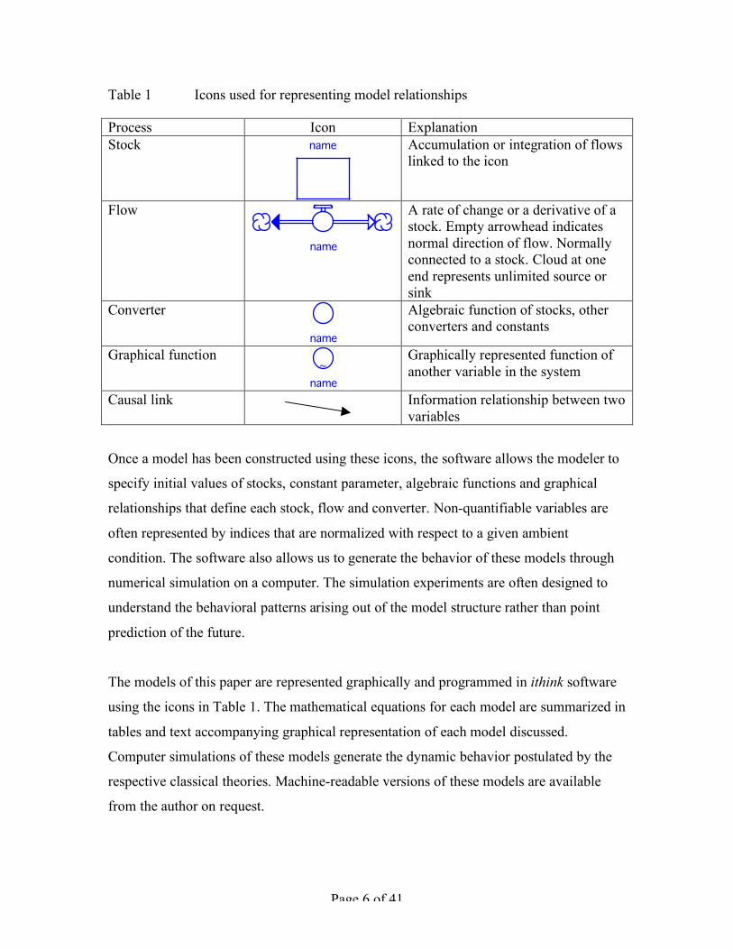
Table 1 Icons used for representing model relationships

Process Icon Explanation Stock name

Accumulation or integration of flows linked to the icon

Flow

name

A rate of change or a derivative of a stock. Empty arrowhead indicates normal direction of flow. Normally connected to a stock. Cloud at one end represents unlimited source or sink

Converter

name

Algebraic function of stocks, other converters and constants

Graphical function ~

name

Graphically represented function of another variable in the system

Causal link

Information relationship between two variables

Once a model has been constructed using these icons, the software allows the modeler to

specify initial values of stocks, constant parameter, algebraic functions and graphical

relationships that define each stock, flow and converter. Non-quantifiable variables are

often represented by indices that are normalized with respect to a given ambient

condition. The software also allows us to generate the behavior of these models through

numerical simulation on a computer. The simulation experiments are often designed to

understand the behavioral patterns arising out of the model structure rather than point

prediction of the future.

The models of this paper are represented graphically and programmed in ithink software

using the icons in Table 1. The mathematical equations for each model are summarized in

tables and text accompanying graphical representation of each model discussed.

Computer simulations of these models generate the dynamic behavior postulated by the

respective classical theories. Machine-readable versions of these models are available

from the author on request.

of 41

Adam Smith and the implicit demographic limit to growth

Although Adam Smith did not clearly discuss the limits to growth, a demographic

constraint is implicit in his model since labor is an autonomous production factor

assumed to be freely available, while capital and technology are endogenously created

through investment of profits (Smith 1977). Also, land which is a proxy for renewable

resources, can be freely substituted by capital (Higgins 1968, pp 56-63), hence it can be

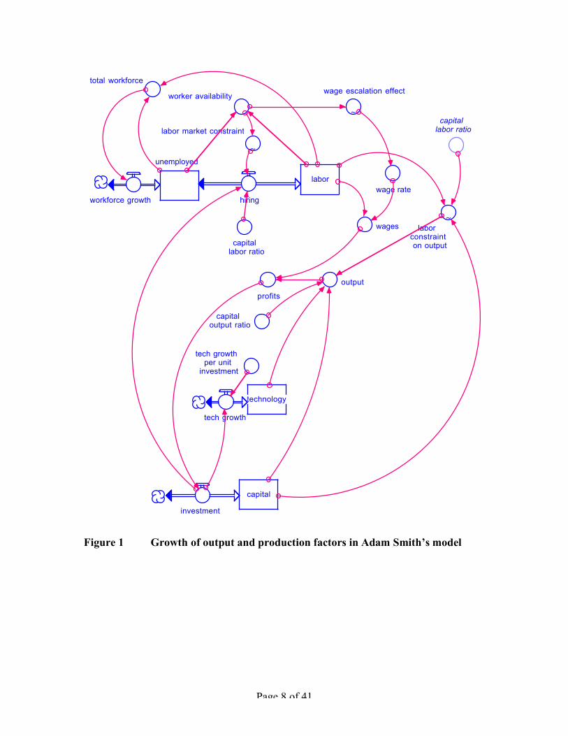
aggregated with capital. Figure 1 represents in system dynamics terms the relationships

between the production factors and the output postulated by Adam Smith.

At the outset, output is created by capital, labor and technology. A labor constraint on

output appears when capital-labor ratio is suboptimal. Capital increases through

investment, which is driven by profits determined by the difference between output and

wage bill. Technological growth is also driven by investment meaning that new capital

formation will upgrade technology. Labor can be hired form a pool of unemployed that is

fed by population growth, while wage depends on the tightness of the labor market.

of 41

capital

investment

output

labor

capital output ratio

technology

tech growth

worker availability

hiring

wages

wage rate

profits

capital labor ratio

~

labor market constraint

tech growth per unit

investment

unemployed

~

wage escalation effect

workforce growth

total workforce

~

labor constraint on output

capital labor ratio

Figure 1 Growth of output and production factors in Adam Smith’s model

of 41

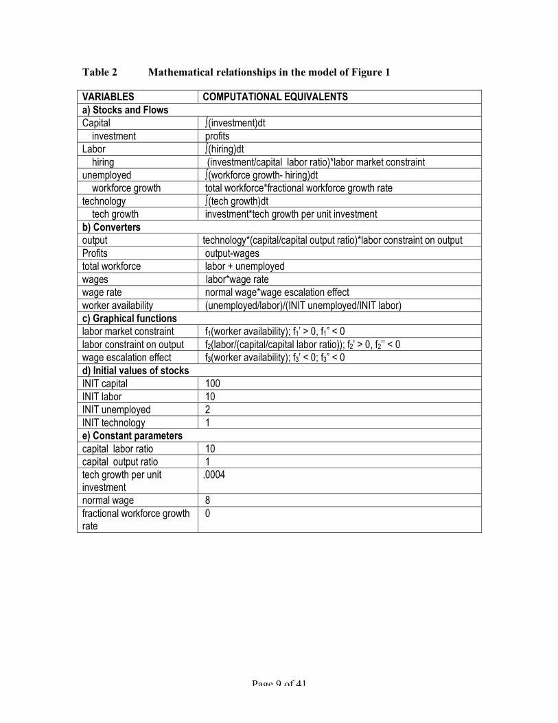
Table 2 Mathematical relationships in the model of Figure 1

VARIABLES COMPUTATIONAL EQUIVALENTS a) Stocks and Flows Capital ∫(investment)dt investment profits Labor ∫(hiring)dt hiring (investment/capital labor ratio)*labor market constraint unemployed ∫(workforce growth- hiring)dt workforce growth total workforce*fractional workforce growth rate technology ∫(tech growth)dt tech growth investment*tech growth per unit investment b) Converters output technology*(capital/capital output ratio)*labor constraint on output Profits output-wages total workforce labor + unemployed wages labor*wage rate wage rate normal wage*wage escalation effect worker availability (unemployed/labor)/(INIT unemployed/INIT labor) c) Graphical functions labor market constraint f1(worker availability); f1’ > 0, f1” < 0 labor constraint on output f2(labor/(capital/capital labor ratio)); f2’ > 0, f2’’ < 0 wage escalation effect f3(worker availability); f3’ < 0; f3” < 0 d) Initial values of stocks INIT capital 100 INIT labor 10 INIT unemployed 2 INIT technology 1 e) Constant parameters capital labor ratio 10 capital output ratio 1 tech growth per unit investment

.0004

normal wage 8 fractional workforce growth rate

0

of 41

Table 2 gives computations underlying each icon in the model of Figure 1. Since a

numerical simulation process is used, the model must be supplied with initial values of

stocks and constant parameters even though we might only be interested in qualitative

patterns of behavior. These values are selected for internal consistency so a hypothetical

homeostasis exists while output exceeds the wage bill thus returning a positive value of

profits.

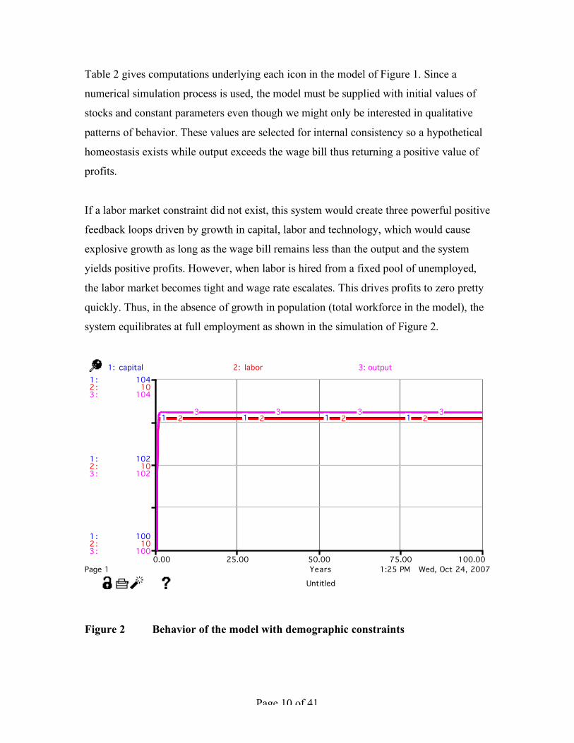
If a labor market constraint did not exist, this system would create three powerful positive

feedback loops driven by growth in capital, labor and technology, which would cause

explosive growth as long as the wage bill remains less than the output and the system

yields positive profits. However, when labor is hired from a fixed pool of unemployed,

the labor market becomes tight and wage rate escalates. This drives profits to zero pretty

quickly. Thus, in the absence of growth in population (total workforce in the model), the

system equilibrates at full employment as shown in the simulation of Figure 2.

1:25 PM Wed, Oct 24, 2007

Untitled

Page 10.00 25.00 50.00 75.00 100.00

Years

1 :

1 :

1 :

2 :

2 :

2 :

3 :

3 :

3 :

100

102

104

10

10

10

100

102

104

1: capital 2: labor 3: output

1 1 1 12 2 2 23 3 3 3

Figure 2 Behavior of the model with demographic constraints

of 41

When land is aggregated with capital in the production schedule, the capital input and the

labor constraint return a Cobb Douglas type production function in which the influence of

technology is autonomous. Growth in any one of the inputs to production can create a

growth in output, however, while Adam Smith gave an endogenous explanation of how

capital and technology grew, he did not discuss any limitations on the growth of labor,

assuming in default that population growth would continue to provide sufficient

quantities of labor so the labor constraint on output does not become active and wage

escalation does not occur. Investment, which is driven by profits, drives all: capital

formation, technological growth and labor hiring.

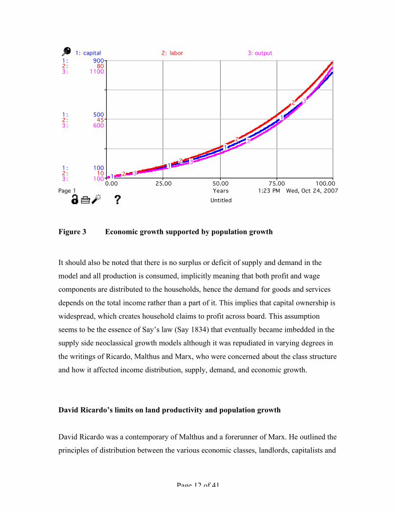
A sustained growth in this system is possible only when a growth in the total workforce

can sustain a pool of unemployed that also keeps wage rate from escalating. Indeed, a

sustained growth is obtained when the model of Figure 1 is simulated with a 2%

workforce growth rate (fractional workforce growth rate is changed to .02). This is shown

in the simulation of Figure 3. Clearly, population growth that creates a growing supply of

labor is critical to maintaining economic growth in Adam Smith’s model. Hence, the

demographic constraint is the unwritten limit to growth since all else is driven by the

profits, which would decline to zero when a tight labor market caused by a fixed

population creates wage escalation.

of 41

1:23 PM Wed, Oct 24, 2007Untitled

Page 10.00 25.00 50.00 75.00 100.00

Years

1 :

1 :

1 :

2 :

2 :

2 :

3 :

3 :

3 :

100

500

900

10

45

80

100

600

1100


1

1

1

1

2

2

2

2

3

3

3

3

Figure 3 Economic growth supported by population growth

It should also be noted that there is no surplus or deficit of supply and demand in the

model and all production is consumed, implicitly meaning that both profit and wage

components are distributed to the households, hence the demand for goods and services

depends on the total income rather than a part of it. This implies that capital ownership is

widespread, which creates household claims to profit across board. This assumption

seems to be the essence of Say’s law (Say 1834) that eventually became imbedded in the

supply side neoclassical growth models although it was repudiated in varying degrees in

the writings of Ricardo, Malthus and Marx, who were concerned about the class structure

and how it affected income distribution, supply, demand, and economic growth.

David Ricardo’s limits on land productivity and population growth

David Ricardo was a contemporary of Malthus and a forerunner of Marx. He outlined the

principles of distribution between the various economic classes, landlords, capitalists and

of 41

workers, which later became important building blocks of the model of growth and

decline of capitalism that Marx conceived. Last, but not least, he brought in the

constraints to growth by stating his law of diminishing returns to land cultivation and the

so-called iron law of wages (Ricardo 1817, McCulloch 1881). These constraints are

added to the model of Figure 1 as follows:

a) Adding Ricardo’s principle of diminishing marginal rents of land

Ricardo’s definition of land rent equated it to land productivity. To quote Ricardo,

Rent is that portion of the produce of the earth which is paid to the landlord for the use of

the original and indestructible powers of the soil. It is often however confounded with the

interest and profit of capital…. (Ricardo 1817, ch. 2).

This means land will need to be disaggregated from capital in the production schedule,

however, for simplification profits and rents can still be aggregated as the two are

residuals after meeting wage bill and running expenses. According to Ricrado,

Whenever, then, the usual and ordinary rate of the profits of agricultural stock, and all

the outgoings belonging to the cultivation of land, are together equal to the value of the

whole produce, there can be no rent. And when the whole produce is only equal in value

to the outgoings necessary to cultivation, there can neither be rent nor profit… (Ricardo

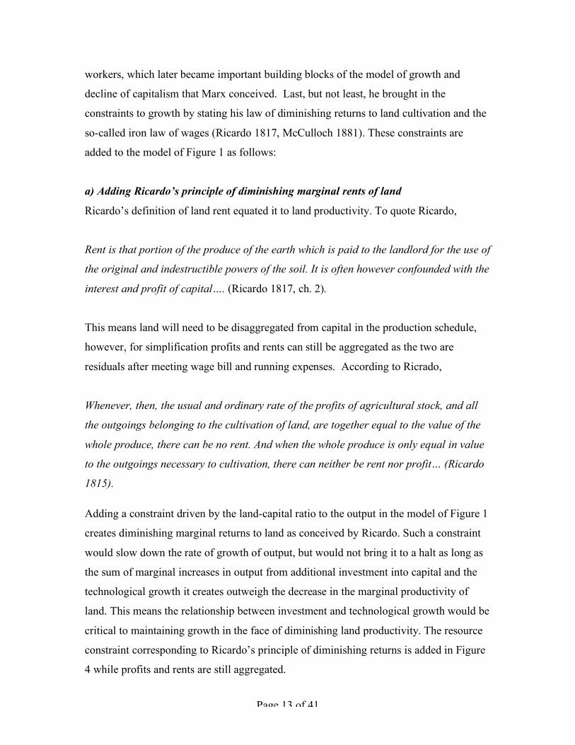
1815). Adding a constraint driven by the land-capital ratio to the output in the model of Figure 1

creates diminishing marginal returns to land as conceived by Ricardo. Such a constraint

would slow down the rate of growth of output, but would not bring it to a halt as long as

the sum of marginal increases in output from additional investment into capital and the

technological growth it creates outweigh the decrease in the marginal productivity of

land. This means the relationship between investment and technological growth would be

critical to maintaining growth in the face of diminishing land productivity. The resource

constraint corresponding to Ricardo’s principle of diminishing returns is added in Figure

4 while profits and rents are still aggregated.

of 41

capital

investment

output

labor


technology

tech growth

worker availability

hiring

wages

wage rate

profitscapital

labor ratio

~



investment

unemployed

~


workforcegrowth

total workforce

Resources ~res constraint

~


capital labor ratio

Figure 4 Ricardo’s law of diminishing land rents (productivity of renewable

resources) added to the model.

of 41

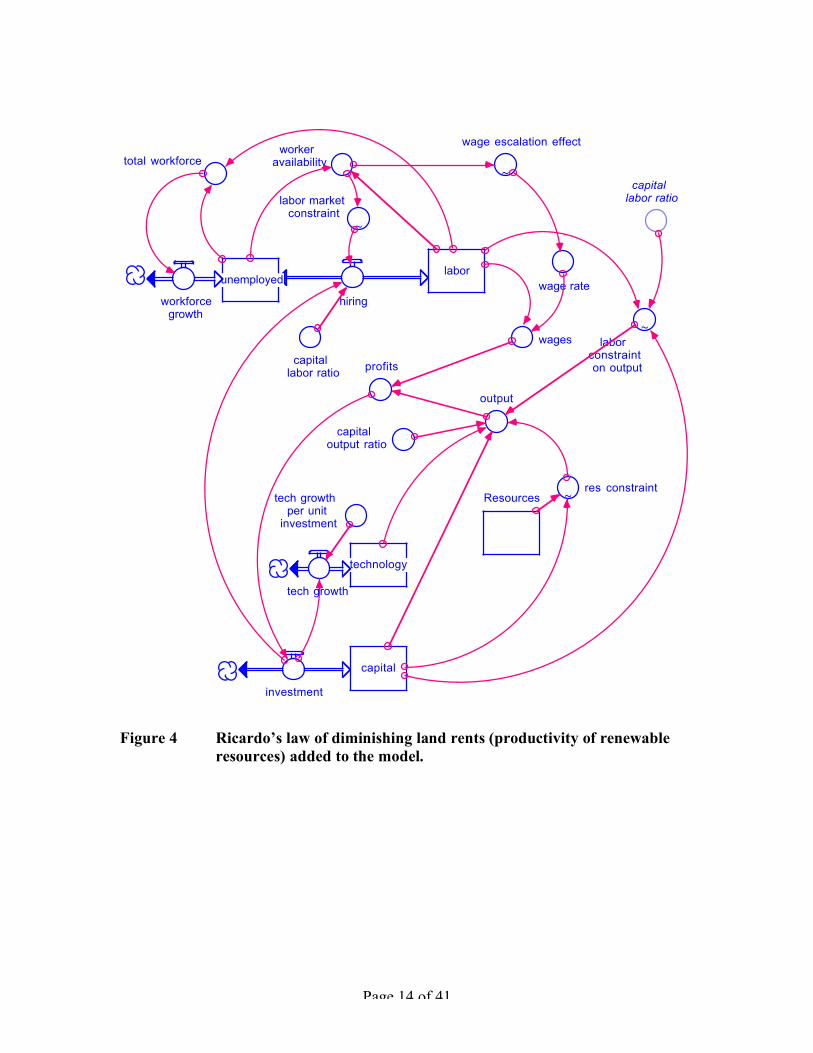
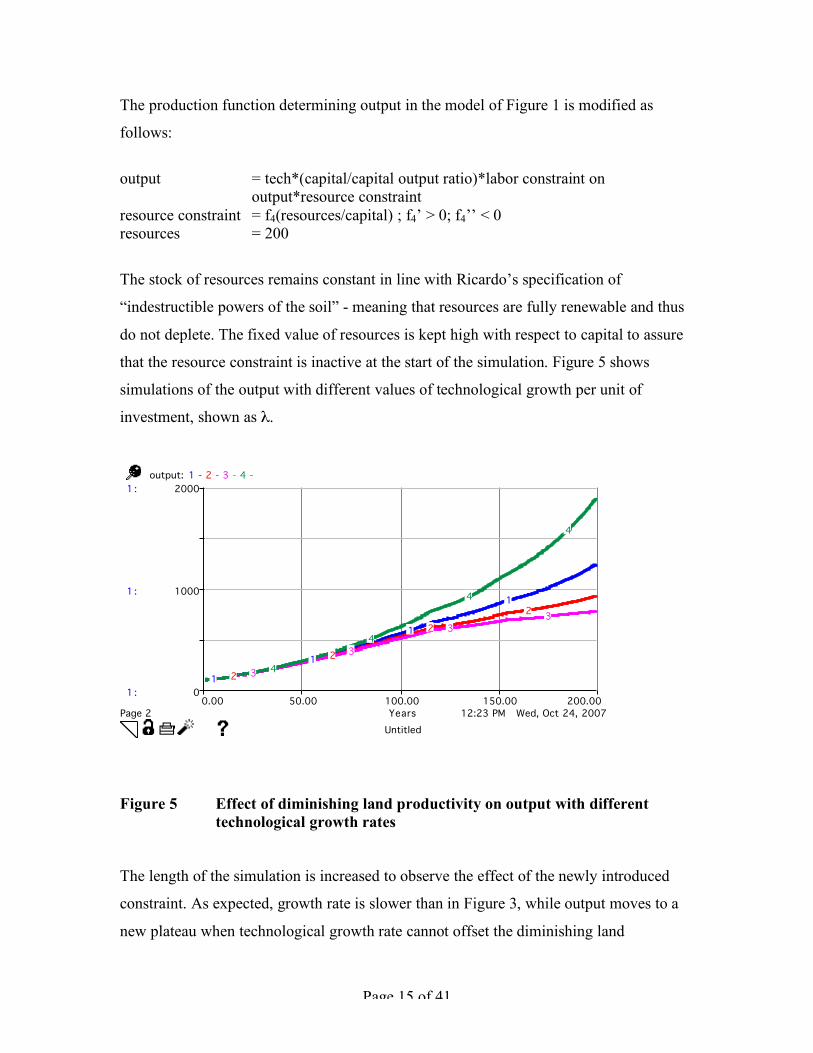
The production function determining output in the model of Figure 1 is modified as

follows:

output = tech*(capital/capital output ratio)*labor constraint on

output*resource constraint resource constraint = f4(resources/capital) ; f4’ > 0; f4’’ < 0 resources = 200

The stock of resources remains constant in line with Ricardo’s specification of

“indestructible powers of the soil” - meaning that resources are fully renewable and thus

do not deplete. The fixed value of resources is kept high with respect to capital to assure

that the resource constraint is inactive at the start of the simulation. Figure 5 shows

simulations of the output with different values of technological growth per unit of

investment, shown as λ.

Figure 5 Effect of diminishing land productivity on output with different technological growth rates

The length of the simulation is increased to observe the effect of the newly introduced

constraint. As expected, growth rate is slower than in Figure 3, while output moves to a

new plateau when technological growth rate cannot offset the diminishing land

12:23 PM Wed, Oct 24, 2007Untitled

Page 20.00 50.00 100.00 150.00 200.00

Years

1 :

1 :

1 :

0

1000

2000output: 1 - 2 - 3 - 4 -

1

1

1

1

2

2

2

2

3

3

33

4

4

4

4

of 41

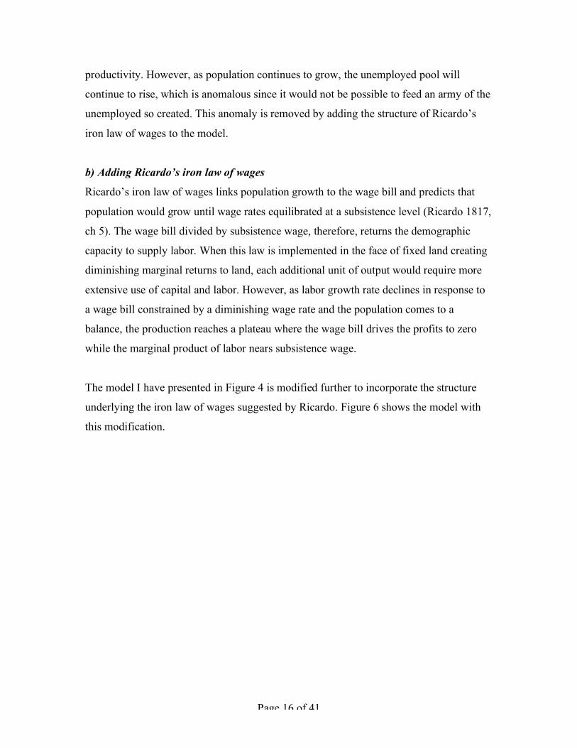
productivity. However, as population continues to grow, the unemployed pool will

continue to rise, which is anomalous since it would not be possible to feed an army of the

unemployed so created. This anomaly is removed by adding the structure of Ricardo’s

iron law of wages to the model.

b) Adding Ricardo’s iron law of wages

Ricardo’s iron law of wages links population growth to the wage bill and predicts that

population would grow until wage rates equilibrated at a subsistence level (Ricardo 1817,

ch 5). The wage bill divided by subsistence wage, therefore, returns the demographic

capacity to supply labor. When this law is implemented in the face of fixed land creating

diminishing marginal returns to land, each additional unit of output would require more

extensive use of capital and labor. However, as labor growth rate declines in response to

a wage bill constrained by a diminishing wage rate and the population comes to a

balance, the production reaches a plateau where the wage bill drives the profits to zero

while the marginal product of labor nears subsistence wage.

The model I have presented in Figure 4 is modified further to incorporate the structure

underlying the iron law of wages suggested by Ricardo. Figure 6 shows the model with

this modification.

of 41

capital

investment

output

labor


technology

tech growth

worker availability

hiring

wages

wage rate

profits

capital labor ratio

~

labor market

constraint


investment

unemployed

worforcecapacity

~


workforce growth

total workforce

Resources ~res constraint

~


capital labor ratio

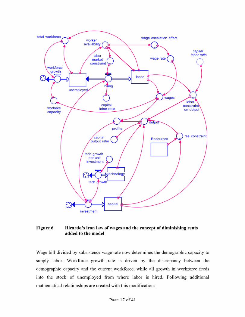
Figure 6 Ricardo’s iron law of wages and the concept of diminishing rents

added to the model Wage bill divided by subsistence wage rate now determines the demographic capacity to

supply labor. Workforce growth rate is driven by the discrepancy between the

demographic capacity and the current workforce, while all growth in workforce feeds

into the stock of unemployed from where labor is hired. Following additional

mathematical relationships are created with this modification:

of 41

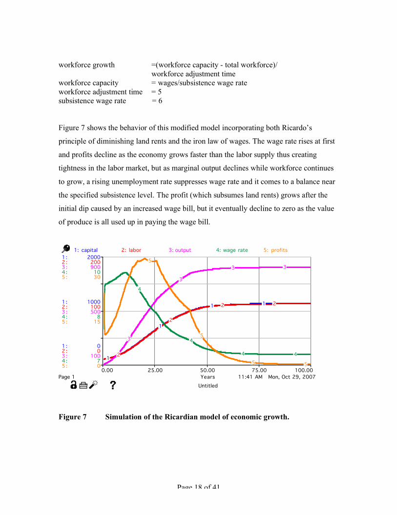
workforce growth =(workforce capacity - total workforce)/ workforce adjustment time workforce capacity = wages/subsistence wage rate workforce adjustment time = 5 subsistence wage rate = 6

Figure 7 shows the behavior of this modified model incorporating both Ricardo’s

principle of diminishing land rents and the iron law of wages. The wage rate rises at first

and profits decline as the economy grows faster than the labor supply thus creating

tightness in the labor market, but as marginal output declines while workforce continues

to grow, a rising unemployment rate suppresses wage rate and it comes to a balance near

the specified subsistence level. The profit (which subsumes land rents) grows after the

initial dip caused by an increased wage bill, but it eventually decline to zero as the value

of produce is all used up in paying the wage bill.

11:41 AM Mon, Oct 29, 2007Untitled

Page 10.00 25.00 50.00 75.00 100.00

Years

1 :

1 :

1 :

2 :

2 :

2 :

3 :

3 :

3 :

4 :

4 :

4 :

5 :

5 :

5 :

0

1000

2000

0

100

200

100

500

900

7

8

10

0

15

30

1: capital 2: labor 3: output 4: wage rate 5: profits

1

1

1 1

2

2

2 2

3

3

3 3

4

4

4 4

5

5

5 5

Figure 7 Simulation of the Ricardian model of economic growth.

of 41

In the final equilibrium, the wage rate equilibrates at near subsistence level, while profits

decline to zero.2 The population has grown to the level determined by the wage bill that

provides enough subsistence to the workers so they can produce, but no not enough for

procreation. Please note that population growth depends on the wage bill only and not on

the total output, which implies that profits are not received by the working households

while capitalist households continue to invest profits until they decline to zero

irrespective of the rate of return on capital. Ricardo did distinguish between “natural” and

“market” prices of commodities meaning that he was are of the imbalance between

supply and demand (Ricardo 1817, ch 4). However, he did not openly repudiate Say’s

law as the production resources in his model always remain fully employed and the

markets apparently clear.

Thomas Malthus, Jay Forrester, population growth and depletion of resources

Thomas Malthus, published ideas similar to Ricardo’s almost simultaneously as Ricardo.

He surmised that population growth by itself is not enough to bring economic advances.

He felt that population growth is an end product in the economic growth process, rather

than a means and posited that an increase in population cannot take place without a

proportionate or nearly proportionate increase of wealth (Malthus 1798). Malthus

repudiated Say’s law by differentiating between the recipients of profits and wages and

emphasizing the importance of demand that is linked mainly to the wage income, but he

did not connect this factor to the demise of capitalism as Marx later posited (Higgins

1968, pp 67-75). Malthus later became concerned with what he described as population

explosion and the scarcity of resources resulting from it (Malthus 1821), and expressed

more or less similar ideas about procreation as Ricardo. The feedback relationship

between population growth and economic growth is however more explicitly addressed 2 There appears what is called in control jargon as steady state error between the nominal and actual values of subsistence wage in my model since the instantaneous rather than the cumulative discrepancy between workforce capacity and population drives population growth. If the discrepancy were integrated in a stock which is then used to drive population growth, the difference between the nominal and steady state values of subsistence wage would disappear, but the growth process would become unstable. This process is called integral control, which is used in Phillip’s stabilization policy (Phillips 1854), but is outside of the scope of the model of this paper.

of 41

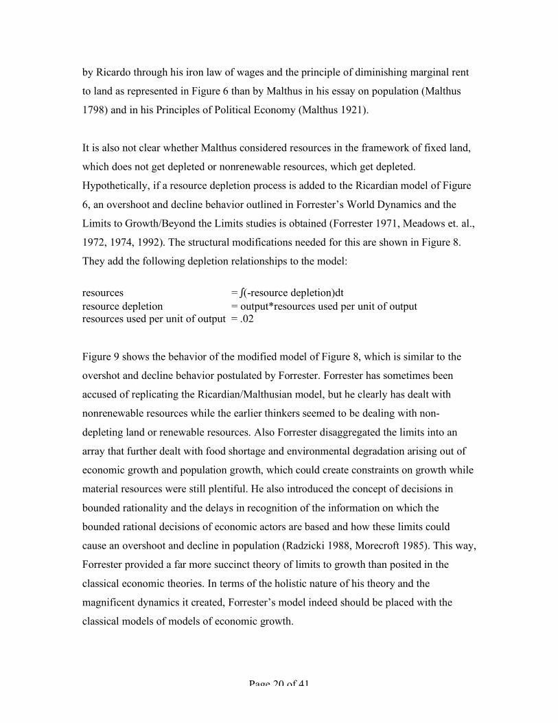
by Ricardo through his iron law of wages and the principle of diminishing marginal rent

to land as represented in Figure 6 than by Malthus in his essay on population (Malthus

1798) and in his Principles of Political Economy (Malthus 1921).

It is also not clear whether Malthus considered resources in the framework of fixed land,

which does not get depleted or nonrenewable resources, which get depleted.

Hypothetically, if a resource depletion process is added to the Ricardian model of Figure

6, an overshoot and decline behavior outlined in Forrester’s World Dynamics and the

Limits to Growth/Beyond the Limits studies is obtained (Forrester 1971, Meadows et. al.,

1972, 1974, 1992). The structural modifications needed for this are shown in Figure 8.

They add the following depletion relationships to the model:

resources = ∫(-resource depletion)dt resource depletion = output*resources used per unit of output resources used per unit of output = .02

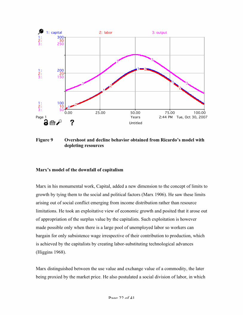
Figure 9 shows the behavior of the modified model of Figure 8, which is similar to the

overshot and decline behavior postulated by Forrester. Forrester has sometimes been

accused of replicating the Ricardian/Malthusian model, but he clearly has dealt with

nonrenewable resources while the earlier thinkers seemed to be dealing with non-

depleting land or renewable resources. Also Forrester disaggregated the limits into an

array that further dealt with food shortage and environmental degradation arising out of

economic growth and population growth, which could create constraints on growth while

material resources were still plentiful. He also introduced the concept of decisions in

bounded rationality and the delays in recognition of the information on which the

bounded rational decisions of economic actors are based and how these limits could

cause an overshoot and decline in population (Radzicki 1988, Morecroft 1985). This way,

Forrester provided a far more succinct theory of limits to growth than posited in the

classical economic theories. In terms of the holistic nature of his theory and the

magnificent dynamics it created, Forrester’s model indeed should be placed with the

classical models of models of economic growth.

of 41

capital

investment

output

labor


tech

tech growth

worker availability

hiring

wages

wage rate

profits

capital labor ratio

~



investment

unemployed

worforce capacity

~


workforce growth

total workforce

Resources

~res constraint

resourcedepletion

~


capital labor ratio

Figure 8 Ricardian/Malthusian model with depleting resources

of 41

2:44 PM Tue, Oct 30, 2007Untitled

Page 10.00 25.00 50.00 75.00 100.00

Years

1 :

1 :

1 :

2 :

2 :

2 :

3 :

3 :

3 :

100

200

300

10

20

30

50

150

250


1

1

1

1

2

2

2

23

3 3

3

Figure 9 Overshoot and decline behavior obtained from Ricardo’s model with depleting resources

Marx’s model of the downfall of capitalism

Marx in his monumental work, Capital, added a new dimension to the concept of limits to

growth by tying them to the social and political factors (Marx 1906). He saw these limits

arising out of social conflict emerging from income distribution rather than resource

limitations. He took an exploitative view of economic growth and posited that it arose out

of appropriation of the surplus value by the capitalists. Such exploitation is however

made possible only when there is a large pool of unemployed labor so workers can

bargain for only subsistence wage irrespective of their contribution to production, which

is achieved by the capitalists by creating labor-substituting technological advances

(Higgins 1968).

Marx distinguished between the use value and exchange value of a commodity, the later

being proxied by the market price. He also postulated a social division of labor, in which

of 41

different people produced different products, so an exchange could occur. As the ultimate

volume of demand for these commodities emerged from the disposable income of the

households, a large pool of unemployed would eventually stifle this demand. Marx thus

clearly repudiated Say’s Law.

Marx also introduced the concept of rate of return on capital which was affected by the

exchange value of commodities. The rate of return influenced the rate of investment.

Marx’s logic is sometimes criticized since in his model investment continues even when

the rate of return turns down. He assumed that available profit will be invested until the

rate of return goes to zero, while profit is the result of the labor performed by the worker

beyond that necessary to create the value of her wages. Thus profit arose out of the

surplus value of labor, which is referred to as the surplus value theory of profit.

This investment structure was, however, consistent with Marx’s distinction between the

capitalists who received all profits and did not have to accrue any capital costs to justify

an investment decision, and the asset-less proletariat who received only wages. Thus,

unlike the neo-classical model, the rate of return in Marx’s model was not the only factor

determining investment. So, even when the rate of return declined, surplus value accrued

as profits needed to be invested. Only when both profits and the rate of return became

zero did the investment finally atrophy. Marx did indeed make the prediction that the rate

of profit will fall over time, and this was one of the factors which led to the downfall of

capitalism. The rate of return declines as the unemployed proletariat is unable to buy the

end commodities and the production capacity cannot be utilized, leading to the creation

of idle capital (Wolff 2003, Higgins 1968, pp 76-87).

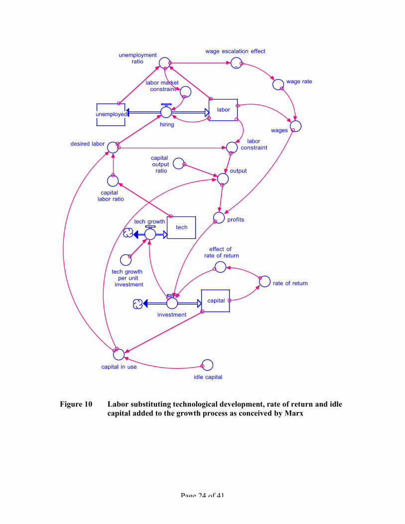
Figure 10 shows the essential structure of Marx’s model that is common to the earlier

models of this paper with the difference that technological development is assumed to be

labor substituting. Output is expressed in terms of use value and even though price is

computed for determining the rate of return on investment, exchange value is not

explicitly represented. Table 3 gives the mathematical relationships underlying the model

structure in Figure 10.

of 41

capital

investment

output

capital in use

labor


techtech growth

unemploymentratio

hiringwages

wage rate

profits

capital labor ratio

desired labor

~

laborconstraint

~



investment

unemployed

~


rate of return

effect of rate of return

idle capital

Figure 10 Labor substituting technological development, rate of return and idle capital added to the growth process as conceived by Marx

of 41

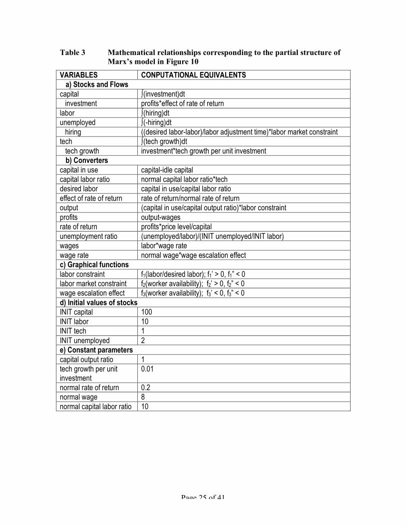
Table 3 Mathematical relationships corresponding to the partial structure of Marx’s model in Figure 10

VARIABLES CONPUTATIONAL EQUIVALENTS a) Stocks and Flows

capital ∫(investment)dt investment profits*effect of rate of return labor ∫(hiring)dt unemployed ∫(-hiring)dt hiring ((desired labor-labor)/labor adjustment time)*labor market constraint tech ∫(tech growth)dt tech growth investment*tech growth per unit investment

b) Converters capital in use capital-idle capital capital labor ratio normal capital labor ratio*tech desired labor capital in use/capital labor ratio effect of rate of return rate of return/normal rate of return output (capital in use/capital output ratio)*labor constraint profits output-wages rate of return profits*price level/capital unemployment ratio (unemployed/labor)/(INIT unemployed/INIT labor) wages labor*wage rate wage rate normal wage*wage escalation effect c) Graphical functions labor constraint f1(labor/desired labor); f1’ > 0, f1” < 0 labor market constraint f2(worker availability); f2’ > 0, f2” < 0 wage escalation effect f3(worker availability); f3’ < 0, f3” < 0 d) Initial values of stocks INIT capital 100 INIT labor 10 INIT tech 1 INIT unemployed 2 e) Constant parameters capital output ratio 1 tech growth per unit investment

0.01

normal rate of return 0.2 normal wage 8 normal capital labor ratio 10

of 41

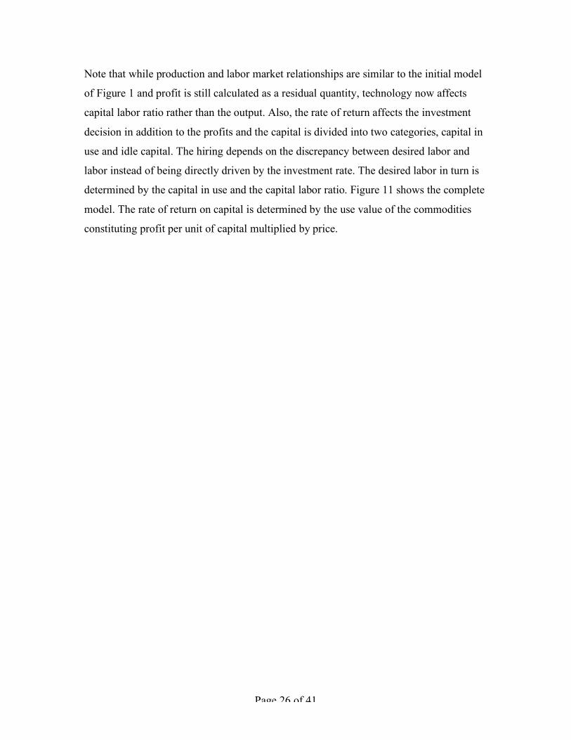
Note that while production and labor market relationships are similar to the initial model

of Figure 1 and profit is still calculated as a residual quantity, technology now affects

capital labor ratio rather than the output. Also, the rate of return affects the investment

decision in addition to the profits and the capital is divided into two categories, capital in

use and idle capital. The hiring depends on the discrepancy between desired labor and

labor instead of being directly driven by the investment rate. The desired labor in turn is

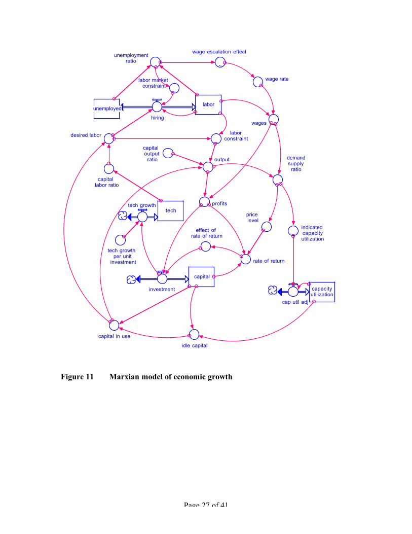
determined by the capital in use and the capital labor ratio. Figure 11 shows the complete

model. The rate of return on capital is determined by the use value of the commodities

constituting profit per unit of capital multiplied by price.

of 41

capital

investment

output

capital in use

labor


techtech growth

unemploymentratio

hiringwages

wage rate

profits

capital labor ratio

desired labor

~

laborconstraint

~



investment

unemployed

~

indicated capacityutilization

~


price level

demandsupplyratio

rate of return


capacityutilization

cap util adj

idle capital

Figure 11 Marxian model of economic growth

of 41

The price in turn depends on supply and demand. Here is where Say’s Law is fully

repudiated. The demand depends on the wage bill while the supply is created by the

capital in use and the employed labor. The capital in use is the difference between the

capital and the idle capital, which depends on capacity utilization. Capacity utilization, in

turn, is determined by the demand relative to the supply over the past period. Population

growth rate is assumed to be zero, while constraints arising from limited resources as

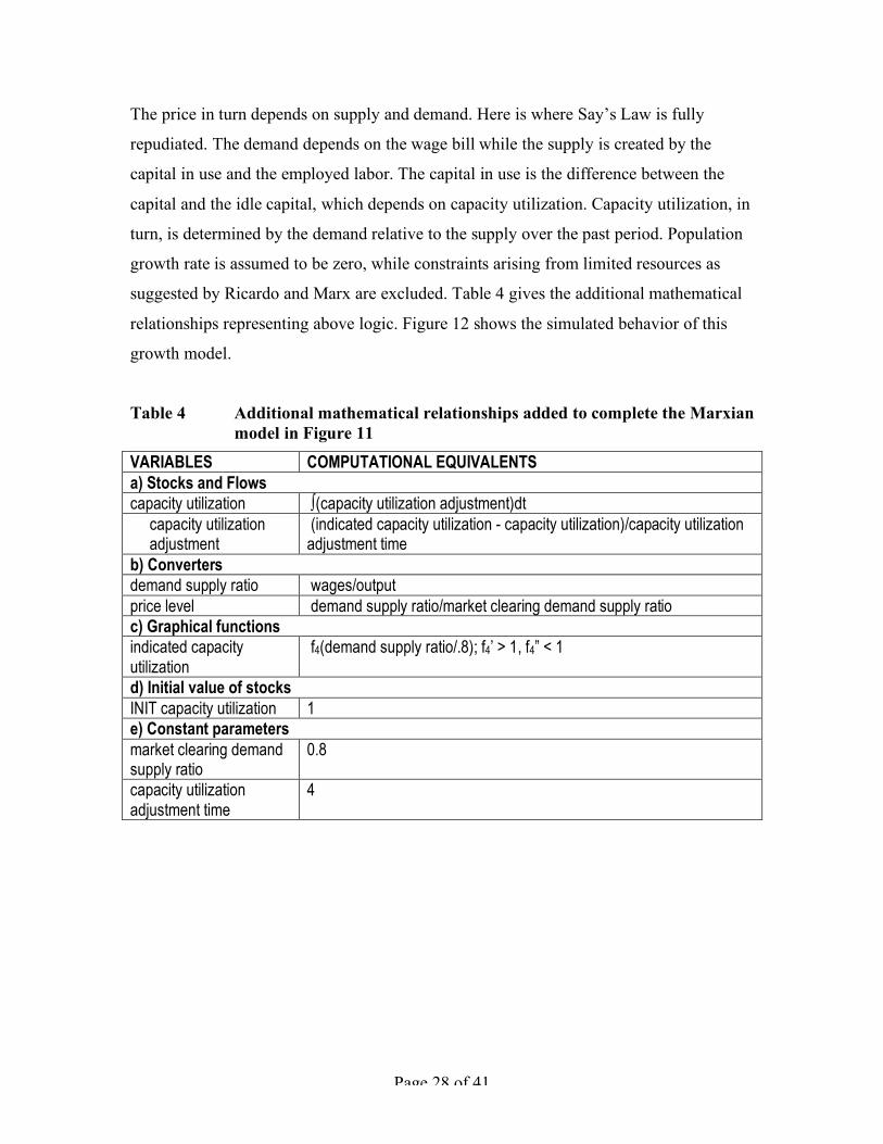
suggested by Ricardo and Marx are excluded. Table 4 gives the additional mathematical

relationships representing above logic. Figure 12 shows the simulated behavior of this

growth model.

Table 4 Additional mathematical relationships added to complete the Marxian model in Figure 11

VARIABLES COMPUTATIONAL EQUIVALENTS a) Stocks and Flows capacity utilization ∫(capacity utilization adjustment)dt capacity utilization adjustment

(indicated capacity utilization - capacity utilization)/capacity utilization adjustment time

b) Converters demand supply ratio wages/output price level demand supply ratio/market clearing demand supply ratio c) Graphical functions indicated capacity utilization

f4(demand supply ratio/.8); f4’ > 1, f4” < 1

d) Initial value of stocks INIT capacity utilization 1 e) Constant parameters market clearing demand supply ratio

0.8

capacity utilization adjustment time

4

of 41

1:01 PM Wed, Sep 19, 2007

Untitled

Page 10.00 5.00 10.00 15.00 20.00

Years

1 :

1 :

1 :

2 :

2 :

2 :

3 :

3 :

3 :

4 :

4 :

4 :

5 :

5 :

5 :

0

500

1000

0

0

0

0

10

20

0

300

600

0

400

800

1: capital 2: rate of return 3: unemployed 4: profits 5: idle capital

1

11 1

2

2 2 2

3

3

33

4

4

4

4

5

5

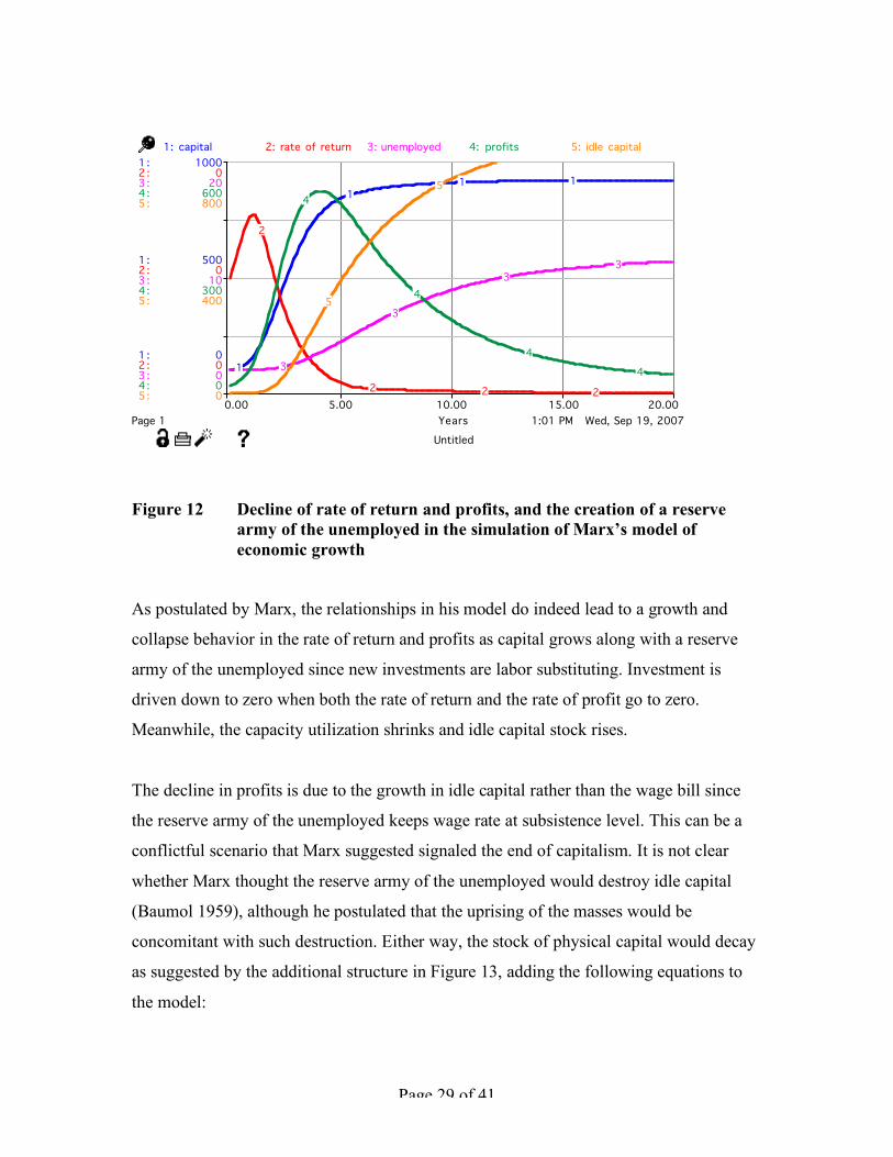
Figure 12 Decline of rate of return and profits, and the creation of a reserve army of the unemployed in the simulation of Marx’s model of economic growth

As postulated by Marx, the relationships in his model do indeed lead to a growth and

collapse behavior in the rate of return and profits as capital grows along with a reserve

army of the unemployed since new investments are labor substituting. Investment is

driven down to zero when both the rate of return and the rate of profit go to zero.

Meanwhile, the capacity utilization shrinks and idle capital stock rises.

The decline in profits is due to the growth in idle capital rather than the wage bill since

the reserve army of the unemployed keeps wage rate at subsistence level. This can be a

conflictful scenario that Marx suggested signaled the end of capitalism. It is not clear

whether Marx thought the reserve army of the unemployed would destroy idle capital

(Baumol 1959), although he postulated that the uprising of the masses would be

concomitant with such destruction. Either way, the stock of physical capital would decay

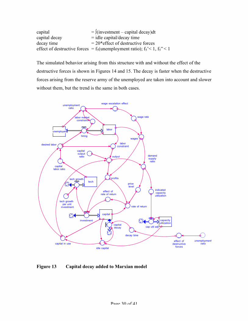
as suggested by the additional structure in Figure 13, adding the following equations to

the model:

of 41

capital = ∫(investment – capital decay)dt capital decay = idle capital/decay time decay time = 20*effect of destructive forces effect of destructive forces = f5(unemployment ratio); f5’< 1, f5” < 1

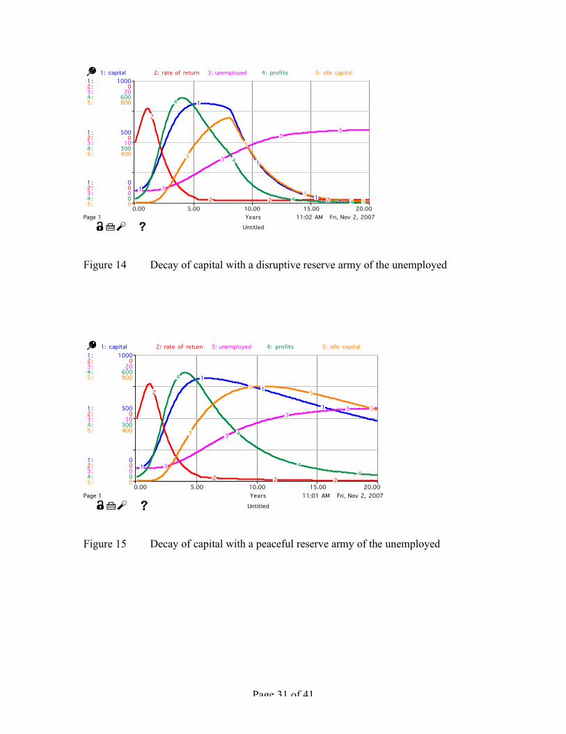
The simulated behavior arising from this structure with and without the effect of the

destructive forces is shown in Figures 14 and 15. The decay is faster when the destructive

forces arising from the reserve army of the unemployed are taken into account and slower

without them, but the trend is the same in both cases.

capital

investment

output

capital in use

labor


techtech growth

unemploymentratio

hiringwages

wage rate

profits

capital labor ratio

desired labor

~

laborconstraint

~



investment

unemployed

~

indicated capacityutilization

~


capitaldecay

price level

demandsupplyratio

rate of return

unemploymentratio

decay time


~

effect ofdestructive

forces

capacityutilization

cap util adj

idle capital

Figure 13 Capital decay added to Marxian model

of 41

11:02 AM Fri, Nov 2, 2007

Untitled

Page 10.00 5.00 10.00 15.00 20.00

Years

1 :

1 :

1 :

2 :

2 :

2 :

3 :

3 :

3 :

4 :

4 :

4 :

5 :

5 :

5 :

0

500

1000

0

0

0

0

10

20

0

300

600

0

400

800


1

1

1

1

2

2 2 2

3

3

33

4

4

4 4

5

5

55

Figure 14 Decay of capital with a disruptive reserve army of the unemployed

11:01 AM Fri, Nov 2, 2007

Untitled

Page 10.00 5.00 10.00 15.00 20.00

Years

1 :

1 :

1 :

2 :

2 :

2 :

3 :

3 :

3 :

4 :

4 :

4 :

5 :

5 :

5 :

0

500

1000

0

0

0

0

10

20

0

300

600

0

400

800


1

1

1

1

2

2 2 2

3

3

33

4

4

44

5

55

5

Figure 15 Decay of capital with a peaceful reserve army of the unemployed

of 41

Schumpeter’s concept of creative destruction and economic cycles

While Marx’s model of destruction of capitalism through exploitation of the proletariat

was based on a class system that locked capitalists and proletariat in separate

compartments, Schumpeter saw the possibility that entrepreneurship could exist across all

social classes. Thus new entrepreneurs could emerge from the ruins of a fallen capitalist

system. They could create a resurgence of capitalism from an environment in which

cheap labor and the possibility of profiting from it would allow them to mobilize idle

capital resources and create new and marketable goods and services from them. In my

observation, Schumpeter saw the possibility of social mobility between classes arising

from entrepreneurship that would rejuvenate a declining capitalist economy, while Marx

had ruled out such mobility. Schumpeter pointed out that entrepreneurs innovate, not just

by figuring out how to use inventions, but also by introducing new means of production,

new products, and new forms of organization. These innovations, he argued, take just as

much skill and daring as does the process of invention (Schumpeter 1962).

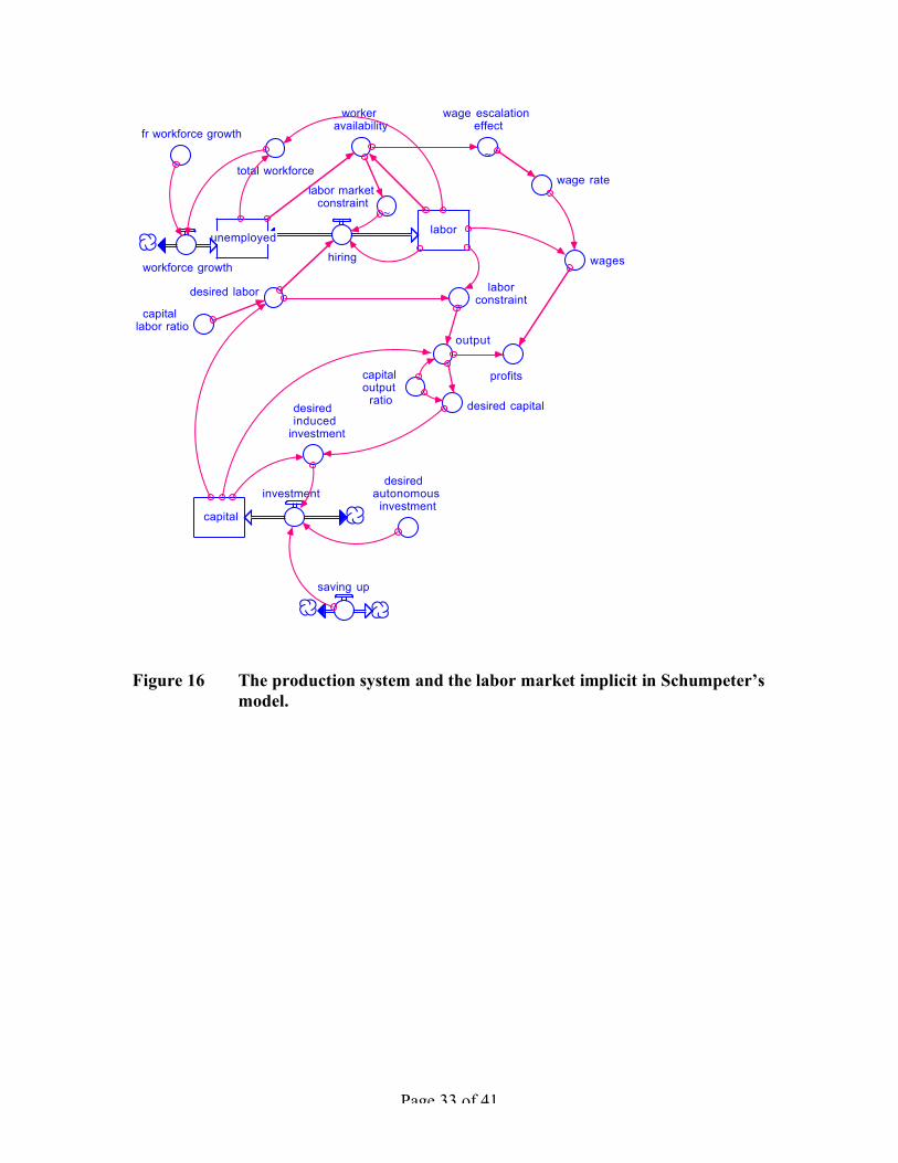
Figure 16 shows the production system and labor market structure implicit in

Schumpeter’s descriptive model as outlined by Higgins (Higgins 1968, pp 88-105).

Please note this structure is more or less similar to Marx with the exception that labor-

substituting characteristic of technology is omitted and the direct link between profits and

investment is deleted. Schumpeter, in fact, distinguished between two types of investment

that he called induced and autonomous. He also introduced a concept of “saving up”

which is different from saving in the neoclassical growth model. Saving up constituted

the part of output that is withheld from investment and consumption. Induced investment

arose from the discrepancy between supply and demand and autonomous investment

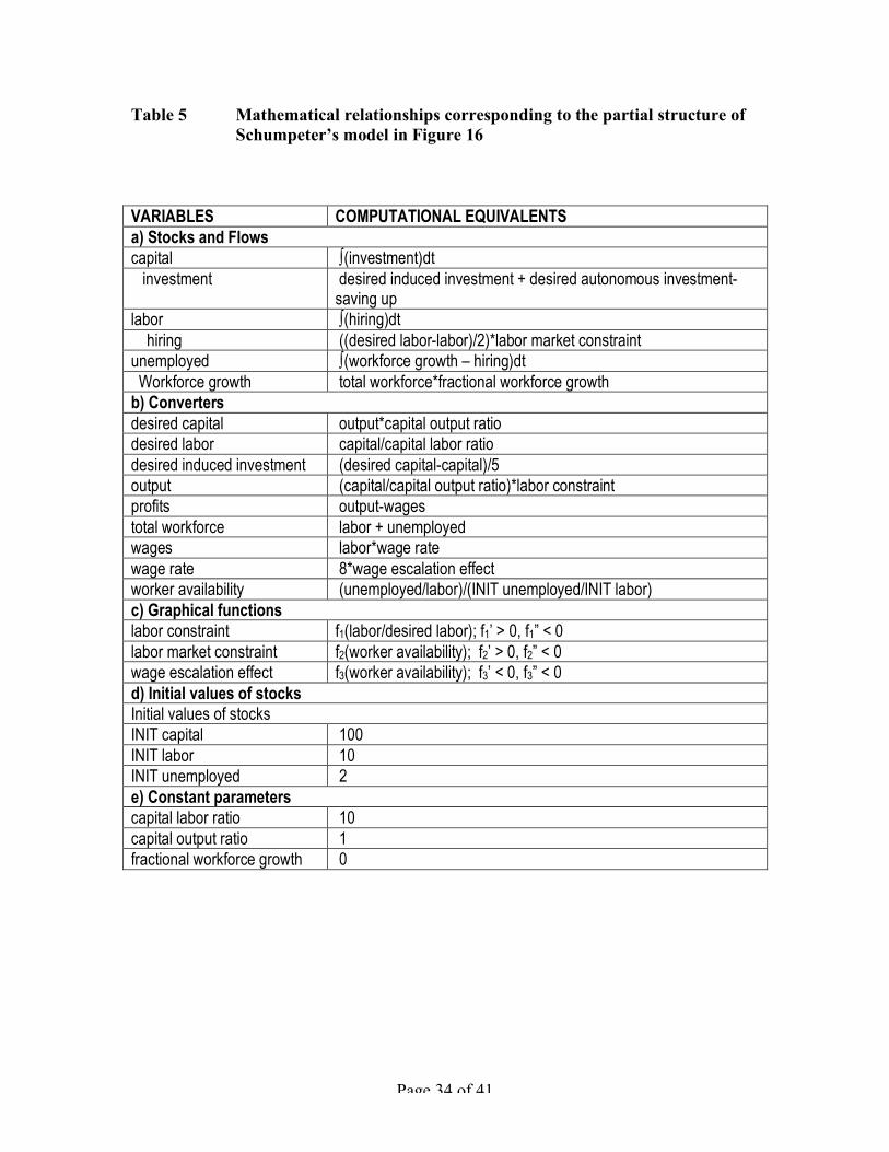
from resources and technology created by the entrepreneurs. Table 5 gives the

mathematical relationships underlying the partial structure of Schumpeter’s model

outlined in Figure 15.

of 41

capital

investment

output

desired induced

investment

labor

desired autonomous investment

capital output

ratio

saving up

worker availability

hiring wages

wage rate

profits

capital labor ratio

desired labor~

laborconstraint

~


unemployed

~


desired capital

workforce growth

total workforce

fr workforce growth

Figure 16 The production system and the labor market implicit in Schumpeter’s model.

of 41

Table 5 Mathematical relationships corresponding to the partial structure of Schumpeter’s model in Figure 16

VARIABLES COMPUTATIONAL EQUIVALENTS a) Stocks and Flows capital ∫(investment)dt investment desired induced investment + desired autonomous investment-

saving up labor ∫(hiring)dt hiring ((desired labor-labor)/2)*labor market constraint unemployed ∫(workforce growth – hiring)dt Workforce growth total workforce*fractional workforce growth b) Converters desired capital output*capital output ratio desired labor capital/capital labor ratio desired induced investment (desired capital-capital)/5 output (capital/capital output ratio)*labor constraint profits output-wages total workforce labor + unemployed wages labor*wage rate wage rate 8*wage escalation effect worker availability (unemployed/labor)/(INIT unemployed/INIT labor) c) Graphical functions labor constraint f1(labor/desired labor); f1’ > 0, f1” < 0 labor market constraint f2(worker availability); f2’ > 0, f2” < 0 wage escalation effect f3(worker availability); f3’ < 0, f3” < 0 d) Initial values of stocks Initial values of stocks INIT capital 100 INIT labor 10 INIT unemployed 2 e) Constant parameters capital labor ratio 10 capital output ratio 1 fractional workforce growth 0

of 41

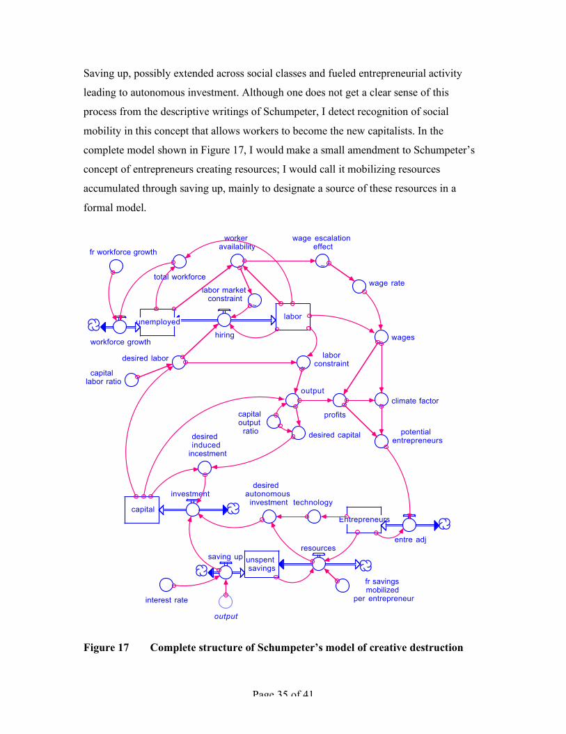
Saving up, possibly extended across social classes and fueled entrepreneurial activity

leading to autonomous investment. Although one does not get a clear sense of this

process from the descriptive writings of Schumpeter, I detect recognition of social

mobility in this concept that allows workers to become the new capitalists. In the

complete model shown in Figure 17, I would make a small amendment to Schumpeter’s

concept of entrepreneurs creating resources; I would call it mobilizing resources

accumulated through saving up, mainly to designate a source of these resources in a

formal model.

capital

investment

output

desired induced

incestment

labor

desired autonomous investment

capital output

ratio

Entrepreneurs

entre adj

saving up

worker availability

hiring wages

wage rate

profits

technology

capital labor ratio

desired labor~

laborconstraint

~


potential entrepreneurs

unemployed

~


desired capital

~climate factor

interest rate

output

fr savings mobilized

per entrepreneur

workforce growth

unspent savings

resources

total workforce

fr workforce growth

Figure 17 Complete structure of Schumpeter’s model of creative destruction

of 41

Both mobilized resources and technology depend on the number of entrepreneurs, which

adjusts towards their potential number determined by profits and entrepreneurial climate.

According to Schumpeter, entrepreneurial climate is created by the availability of a high

rate of profits and the availability of cheap labor. I have accumulated the difference

between the saving up, which Schumpeter said depended on interest rate, and the

mobilized resources in a stock of unspent savings, which supply the venture capital for

the entrepreneurs. This also allows the model to have a hypothetical equilibrium in which

induced investment is zero and saving up equals the resources mobilized by the

entrepreneurs or the venture capital investment. Table 6 shows additional mathematical

relationships corresponding to the additional structure in Figure 17.

of 41

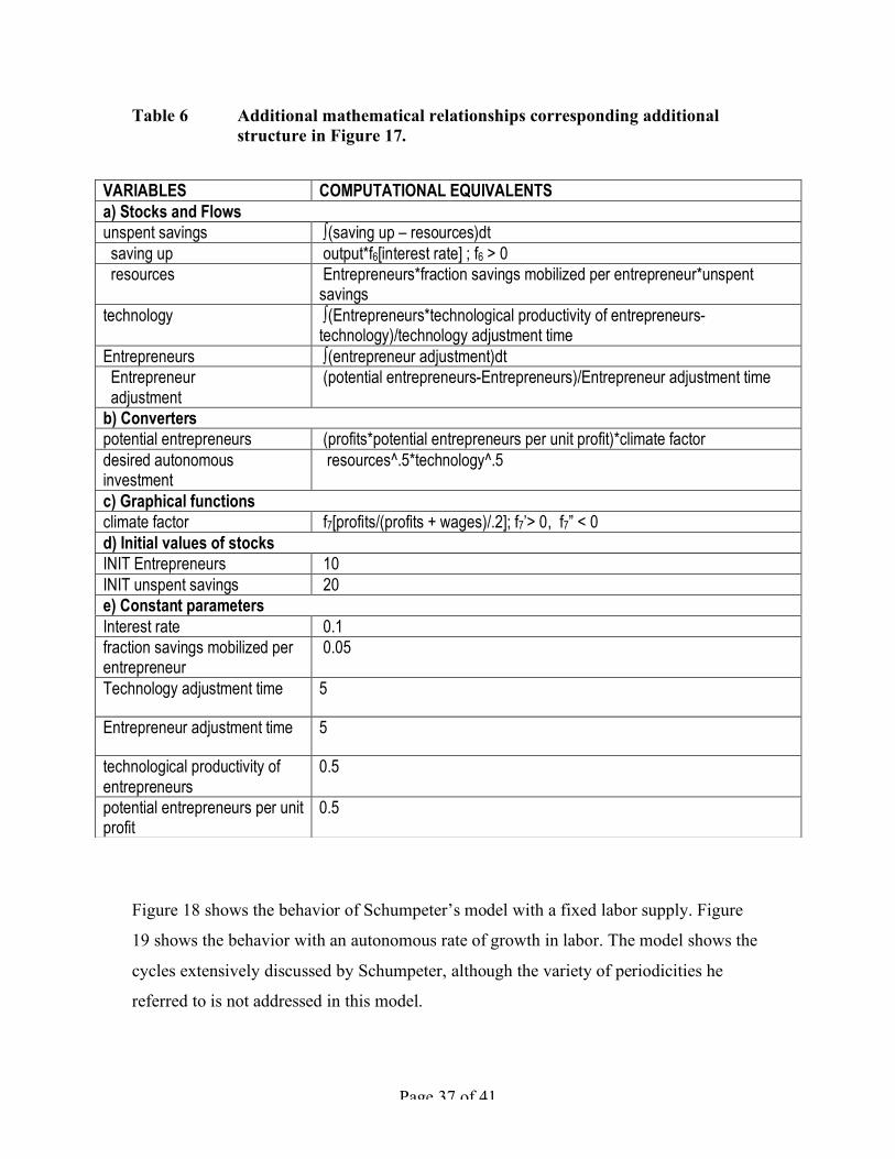
Table 6 Additional mathematical relationships corresponding additional structure in Figure 17.

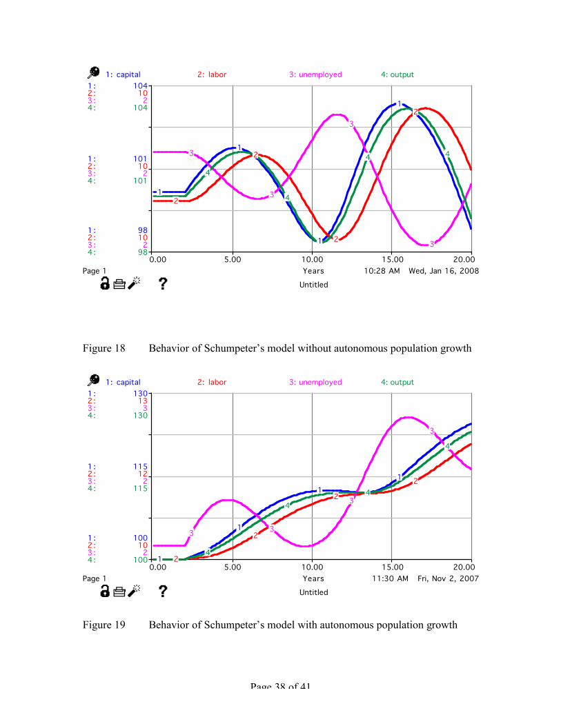
Figure 18 shows the behavior of Schumpeter’s model with a fixed labor supply. Figure

19 shows the behavior with an autonomous rate of growth in labor. The model shows the

cycles extensively discussed by Schumpeter, although the variety of periodicities he

referred to is not addressed in this model.

VARIABLES COMPUTATIONAL EQUIVALENTS a) Stocks and Flows unspent savings ∫(saving up – resources)dt saving up output*f6[interest rate] ; f6 > 0 resources Entrepreneurs*fraction savings mobilized per entrepreneur*unspent

savings technology ∫(Entrepreneurs*technological productivity of entrepreneurs-

technology)/technology adjustment time Entrepreneurs ∫(entrepreneur adjustment)dt Entrepreneur adjustment

(potential entrepreneurs-Entrepreneurs)/Entrepreneur adjustment time

b) Converters potential entrepreneurs (profits*potential entrepreneurs per unit profit)*climate factor desired autonomous investment

resources^.5*technology^.5

c) Graphical functions climate factor f7[profits/(profits + wages)/.2]; f7’> 0, f7” < 0 d) Initial values of stocks INIT Entrepreneurs 10 INIT unspent savings 20 e) Constant parameters Interest rate 0.1 fraction savings mobilized per entrepreneur

0.05

Technology adjustment time 5

Entrepreneur adjustment time 5

technological productivity of entrepreneurs

0.5

potential entrepreneurs per unit profit

0.5

of 41

10:28 AM Wed, Jan 16, 2008

Untitled

Page 10.00 5.00 10.00 15.00 20.00

Years

1 :

1 :

1 :

2 :

2 :

2 :

3 :

3 :

3 :

4 :

4 :

4 :

98

101

104

10

10

10

2

2

2

98

101

104

1: capital 2: labor 3: unemployed 4: output

1

1

1

1

2

2

2

2

3

3

3

3

4

4

4 4

Figure 18 Behavior of Schumpeter’s model without autonomous population growth

11:30 AM Fri, Nov 2, 2007

Untitled

Page 10.00 5.00 10.00 15.00 20.00

Years

1 :

1 :

1 :

2 :

2 :

2 :

3 :

3 :

3 :

4 :

4 :

4 :

100

115

130

10

12

13

2

2

3

100

115

130

1: capital 2: labor 3: unemployed 4: output

1

1

11

2

2

2

2

3 3

3

3

4

44

4

Figure 19 Behavior of Schumpeter’s model with autonomous population growth

of 41

The autonomous investment arising from entrepreneurial creativity creates competition

that expands creative activity and shrinks profits, while creating tightness in the labor

market that takes away the very elements of the entrepreneurial environment that helped

launch it. Schumpeter called this process the “creative destruction” and postulated that

this would result in a cyclical tendency in the capitalist system, which is indeed borne out

buy the simulation of his model. Although Schumpeter referred to many types of

economic cycles in his writings the feedback processes distinguishing their periodicities

are not clear. The model I have constructed exhibits a periodicity of about 10 years based

on the time constants I have selected, while it specifically addresses the process of

creative destruction that Schumpeter originally posited.

Conclusion

The concept of limits was tightly interwoven with the process of growth postulated in the

classical theories. These limits encompassed many domains including demographic,

environmental, social and political. In most instances, the recognition of these limits

required dealing with soft variables that were difficult to quantify in the neoclassical

analysis tradition. It is not surprising that these processes have been excluded from the

formal analyses of mainstream economics, which has greatly reduced the explanatory

power of the neoclassical theory, which has come to attribute all deviations from the

postulated behavior of a hypothetical perfect market system to the imperfections in the

reality, which is a violation of the scientific principles of modeling. All models are

wrong, only reality is right and first requirement of a model is to replicate some aspect of

reality before it can be accepted as a basis for a policy intervention.

Classical economics, on the other hand did attempt to replicate empirical realism in its

theories often using soft variables in its explications. System dynamics modeling allows

reinstatement of such soft variables in our models of economic behavior that should

reincarnate the rich insights the traditional economic concepts provided. This indeed

requires reinventing modern economics, which should be undertaken without further

delay.

of 41

References Baumol, William. 1959. The Classical Dynamics. In Economic Dynamics. 2nd ed. Ch 2:

13-21. New York: The Macmillan Company Devarajan, S. and A. Fisher. 1981. Hotelling’s “Economics of Exhaustible Resources”:

Fifty Years Later. Journal of Economic Literature. 19(1): 65-73. Forrester, J W. 1971. World Dynamics. Cambridge, MA: MIT Press. Forrester, J W. 1961. Industrial Dynamics. Cambridge, MA: MIT Press. Forrester, J W. 1979. An Alternative Approach to Economic Policy: Macrobehavior

from Microstructure. In Nake M. Kamrany and Richard H. Day (Eds.), Economic Issues of the Eighties. Baltimore: Johns Hopkins University Press. pp. 80-108.

Forrester, Nathan. 1973. The Life Cycle of Economic Growth. Walthum, MA: Pegasus Communications

Hartwick. John M. 1977. Intergenerational Equity and Investing Rents from Exhaustible Resources. American Economic Review. 67(5): 972-974.

Hielbroner, R. L. 1980. The Worldly Philosophers. Fifth Edition. New York: Simon & Schuster.

Higgins, Benjamin, 1968. Economic Development, Problems, Principles and Policies. New York: W. W. Norton.

High Performance Systems. 1997. STELLA Research Applications. Hanover NH: High Performance Systems. pp 87-107

Hotelling, Harold. 1931. The Economics of Exhaustible Resources. Journal of Political Economy. 39(2): 137-175.

Malthus, Thomas R. 1798. First Essay on Population. Royal Economic Society (Great Britain, Published in 1926). London: Macmillan Publishing Co.

Malthus, Thomas. 1821. Principles of Political Economy, Considered With a View to Their Practical application. London: Wells and Lilly.

Marx, Karl. 1906. Capital, A Critique of Political Economy. Fredrick Engles (ed.). New York: Random House, Charles H. Kerr and Company.

Mass, N. J. 1975. Economic Cycles: An Analysis of Underlying Causes. Cambridge MA: Productivity Press.

McCulloch, J. R. (Ed.). 1881. The Works of David Ricardo. London: John Murray. pp31, 50-58.

Meadows, Dennis, et. al. 1974. Dynamics of Growth in a Finite World. Cambridge, MA: MIT Press

Meadows, Donella, Dennis Meadows and Jorgan Randers. 1992. Beyond the Limits. Post Mills, Vermont: Chelsea Green Publishing Co.

Meadows, Donella, et. al. 1972. The Limits to Growth. New York: Universe Books. Morecroft, John D. W. 1985. Rationality in the Analysis of Behavioral Simulations.

Management Science. 31(3): 900-916. Nordhaus, W. D. 1964. Resources as a Constraint. American Economic Review. 64(2):

22-26. Nordhaus, W. D. 1979. The Efficient Use of Energy Resources. Cowles Foundation, New

Haven, CT: Yale University Press.

of 41

Phillips, A.W. 1954. Stabilization Policy in a Closed Economy. Economics Journal. 64: 290-323

Radzicki, M J. 1988. Institutional Dynamics: An Extension of the Institutional Approach to Socioeconomic Analysis. Journal of Economic Issues. 22(3): 633-665.

Ricardo, David. 1815. An Essay on Profits. London: Printed for John Murray, Albemarle Street.

Ricardo, David. 1817. On Principles of Political Economy and Taxation. Kitchener, Ontario, Canada: Batoche Books. 2001.

Saeed, K. 1985. An Attempt to Determine Criteria for Sensible rates of Use of Material Resources. Technological Forecasting and Social Change. 28(4).

Saeed, K. 1994. Development Planning and Policy Design: A System Dynamics Approach. Aldershot, England: Ashgate/Avebury Books.

Say, J B. 1834. A treatise on political economy, or production, distribution and consumption of wealth. (Translation from French by C R Princep). Philadelphia, PA: Grigg and Elliot

Schumpeter, Joseph A. 1962. Capitalism, Socialism and Democracy. New York: HarperCollins.

Smith, Adam. 1977. Inquiry Into the Nature and Causes of the Wealth of Nations. Chicago: University of Chicago Press

Smith, V K and Krutilla, J V. 1984. The American Economic Review. 72(2): 226-230. Solow, Robert M. 1974. The Economics of Resources or Resources of Economics.

Richard T. Ely Lecture. American Economic Review. 64(2): 1-14. Solow, Robert M. 1986. Growth and Distribution: Intergenerational Problems. The Scandinavian Journal of Economics, 88(1): 141-149 Street, J H. 1983. The Reality of Power and the Poverty of Economic Doctrine. Journal

of Economic Issues. 17(2):295-311 Wolff, Jonathan, "Karl Marx", The Stanford Encyclopedia of Philosophy (Fall 2003

Edition), Edward N. Zalta (ed.). URL = <http://plato.stanford.edu/archives/fall2003/entries/marx/>.

Limits to Growth Concepts in Classical Economics Revised ... · PDF fileLimits to Growth...

Documents

Transcript of Limits to Growth Concepts in Classical Economics Revised ... · PDF fileLimits to Growth...