Limited Re-Sequencing for Mixed-Models with Multiple...

American Journal of Operations Research, 2012, 2, 10-21 http://dx.doi.org/10.4236/ajor.2012.21002 Published Online March 2012 (http://www.SciRP.org/journal/ajor)

Limited Re-Sequencing for Mixed-Models with Multiple Objectives, Part II: A Permutation Approach

Patrick R. McMullen Schools of Business, Wake Forest University, Winston-Salem, USA

Email: [email protected]

Received October 31, 2011; revised November 28, 2011; accepted December 13, 2011

ABSTRACT

This research presents an approach to solving the limited re-sequencing problem for a JIT system when two objectives are considered for multiple processes. One objective is to minimize the number of setups; the other is to minimize the material usage rate [1]. For this research effort, each unique permutation of the problem’s demand structure is noted, and used as a mechanism for finding subsequent sequences. Two variants of this permutation approach are used: one employs a Monte-Carlo simulation, while the other employs a modification of Ant-Colony Optimization to find se-quences satisfying the objectives of interest. Problem sets from the literature are used for assessment, and experimenta-tion shows that the methodology presented here outperforms methodology from an earlier research effort [2]. Keywords: Permutation; Heuristic; Sequencing; Discrete Optimization

1. Introduction

Prudent production scheduling has long been a means for enhancing the competitive position of the manufacturing firm. Effective scheduling can be used to enhance flexi-bility in a Just-in-time (JIT) system, as well as reduce the required number of setups associated with changeovers. These two entities (flexibility and required number of setups) are of paramount concern here. Many past re-search efforts have confirmed the fact that these two en-tities are inversely related to each other. In other words, a strong performance of one suggests a poor performance of the other.

Another caveat related to production sequencing re-lates to the fact that there are frequently several individ-ual processes involved in the aggregate production func-tion. For each individual process, it may be possible to “re-sequence” the production sequence used in the prior stage of production. This re-sequencing may, if properly done, induce some efficiencies that were not present be-fore re-sequencing. Exploiting the multiple processes with the intent of performing well with regard to both number of setups and flexibility is a facet of production research that has not been explored to any reasonable degree.

This research addresses the production sequencing problem in a JIT environment where the number of set-ups and the flexibility of the sequences are simultane-ously considered for multiple processes. Two heuristics are presented to accomplish the sequencing—both are

rooted in a Monte-Carlo simulation selection process. The first employs a selection process rooted in perform-ance potential, the second employs the same selection process as the first, but is also weighted in the spirit of Ant Colony Optimization [3]. For a set of problems from the literature, the performance of the heuristics is as-sessed against optimal, and against a search heuristic from a prior research effort [2].

Via development of a detailed example detailing the concept of limited re-sequencing and capturing the effi-cient frontier, the sequencing methodology is presented, an experiment is described, analyses of performance are made, and general observations are offered.

2. Sequencing and Limited Re-Sequencing

2.1. Setups vs. Flexibility

To better understand the idea of multiple objectives and multiple processes, consider a trivial problem that re-quires two units of item A, one item of item B, and one unit of item of C to be placed into a production sequence. On possible sequence is AABC. This sequence results in (3) changeovers, which is the minimum value possible. Unfortunately, this sequence does not propagate flexibil-ity—there is an uneven flow of items through the se-quence, in proportion to demand, resulting in a high us-age rate (2.75) as presented by Miltenburg [1]. Although the usage rate is formally defined in the methodology section, an informal description is provided here. Con-sider a hypothetical situation where the two units of A,

Copyright © 2012 SciRes. AJOR

P. R. MCMULLEN 11

and single units of B and C are required for the cus-tomer’s to assemble. If the total number of demanded assemblies is 10,000 units, then 20,000 units of A would be required, with 10,000 units of both B and C required. Suppose the schedule is to produce the 20,000 units of A, followed by the 10,000 units of B, and finishing with the 10,000 units of C. This sequence would result in (3) set-ups—the minimum possible amount. Consider next, some sort of disaster, such as a massive power outage, occurring immediately after the 20,000 units of A were produced. These completed units of item A are of no value to the customer, because items B and C are un-available and required for the assembly. This hypotheti-cal scenario illustrates a lack of flexibility, underscoring the importance of “inter-mixing” the individual items as much as possible—an important feature of JIT systems.

One sequence that would better propagate flexibility is ABAC. This sequence has a better measure of usage (1.75) than does AABC. Unfortunately, this sequence requires (4) setups, more than the (3) associated with the AABC sequence. This scenario illustrates that a sequence boasting flexibility can result in more setups than a se-quence involving less flexibility. This inverse relation-ship between required setups and flexibility (measured via Miltenburg’s usage rate) is a complicating force in production scheduling.

2.2. Multiple Processes

Another complicating force is the requirement of multi-ple processes. Consider the above example applied to multiple processes. For the purpose of this illustration, it is assumed that (10) processes are required. The AABC sequence would then require (30) setups in all, with an aggregate usage measure of 27.5. The ABAC sequence would require (40) setups, with an aggregate usage measure of 17.5. The AABC sequence provides desirable setups, but undesirable flexibility, while the ABAC se-quence provides just the opposite returns.

2.3. Limited Re-Sequencing

It appears that the multiple processes further amplify the tradeoff between setups and flexibility. This need not be the case if one were to “re-sequence” items between the different processes. In this context, re-sequencing means that one item is taken out of the sequence, and re-inserted into a later part of the sequence. Consider the following example of re-sequencing, where item B (underlined) is re-inserted into a later part of the sequence.

AABC (Original Sequence)

AACB (Modified Sequence)

In the example above, item B was physically removed from the sequence, held in a buffer, and later re-inserted

[4]. This type of re-sequencing suggests the assumption that there is physical space available that permits one to hold an item in a buffer until a later time. Specifically, this research does permit a buffer size of one unit, essen-tially meaning that one unit can be held and later re-inserted in the sequence. A side effect of this assump-tion is that units not held in buffer can move up no more than one sequence position. Below is an example of a forbidden sequence modification:

AABC (Original Sequence)

BCAA (Modified Sequence)

The above scenario is more permitted because both of the items A would have been held in buffer (exceeding the buffer size of one), causing the B and C to move up more than one position in the sequence. Finally, it is permitted to have more than one modifications made in a sequence, provided that there is never more than one unit held in buffer at a time. Here is an example of this:

ABAC (Original Sequence)

BACA (Modified Sequence)

The above sequence modification is permitted because there is at most one unit held in buffer at any time (it is item A in this example). The first item A is held in buffer and is re-inserted after item B. The second item A is held in buffer and is re-inserted after item C. Note that neither items B or C more up more than one sequence position. This re-sequencing preserves diversity in the continuum of feasibility [5].

2.4. Seeking an Efficient Frontier

As stated earlier, the minimum setups sequence is AABC, resulting in (3) setups and a usage rate of 2.75. Another sequence is ABAC, resulting in (4) setups and a usage rate of 1.75. Applied over (10) total processes, AABC yields 30 total setups and an aggregate usage of 27.5. The ABAC sequence, over (10) processes yields 40 total setups and an aggregate of usage of 17.5.

In the interest of multiple objectives, it is germane to seek sequences that find some “middle ground” between the extreme values of setups and usage rates. This “middle ground” can be found via an efficient frontier. In the context of this application, an efficient frontier is in- tended to describe the minimum usage rate for each unique number of setups for the total number of processes. For problems such as this, where one objective is of a discrete nature (number of required setups) and the other is continuous (the associated usage rate), an efficient frontier works well.

Finding this efficient frontier is a non-trivial task, and is, in effect, one of the main contributions of this research effort. In order to find the efficient frontier, one must find the set of sequences that yield the minimum


P. R. MCMULLEN


12

cussed in the methodology section. For now, the usage rates and setups are shown in Table 1 for all twelve pos-sible permutations of the AABC problem.

total usage rate for their associated number of required setups/changeovers. For this research, the “trivial,” or “level-0” sequence will always be the one with the item As at the head of the sequence, followed by the items Bs, etc. For each process required, the prior level’s sequence is subjected to limited re-sequencing as described above. One of the candidate sequences is selected and this proc-ess continues until the desired number of levels has re-ceived proper attention.

Also shown in Table 1 is information regarding feasi-bility of child sequences descending from parent se-quences. A mark of “1” indicates feasibility from parent to child sequence, a mark of “0” indicates infeasibility. For example, the above elaboration of the feasible child sequences of AABC are noted with marks of “1” in Ta-ble 1 (shaded—“ID” tags must be referenced). There are essentially two general ways of capturing

the efficient frontier. One way is via enumeration, the other way is via some heuristic search. The enumerative approach is guaranteed optimal, but expensive in terms of effort. The heuristic approach is not guaranteed opti-mal, but if wisely pursued, it can provide near-optimal results with a reasonable effort. For an enumerative effort, one must traverse a search tree, where the nodes are the parent sequence, and the branches are the feasible child sequences of the parent sequences. For the child se-quences to be feasible, they must have their sequence members move up at most one position in the sequence. For example, the “level-0” sequence of AABC only has four feasible child sequences: AABC, AACB, ABAC and ABCA. Each of these child sequences then exist at level 1, and each of these are then considered parent se-quences for level 2, etc.

If the traversal process were continued through ten processes, the efficient frontier would appear as shown in Figure 2.

While inspection of Figure 2 shows the graphical rela-tionship between setups and usage rate, Table 2 shows the specific sequences that make up the efficient frontier. Here, the interested reader can see the exact sequences that make up the efficient frontier. For example, the combinations of sequences that comprise the lowest us-age for 39-setups are BAAC for Level 1, ABCA for Level 2, etc.

2.5. Combinatorial Explosion

Figure 1 shows the traversal details that are essentially required to find the efficient frontier through two levels. Even for two levels, the effort is consequential. Level 0 has a single node, Level 1 has four nodes, Level 2 has twenty-nodes. This illustrates a combinatorial explosion.

Figure 1 shows cumulative usage and setups through each path of the traversal. While the required setups are easily understandable, usage rate is less so, and is dis-

Figure 1. Tree diagram of AABC: Full enumeration through two processes (p = 2). Cumulative setups (S) and usage (U) are shown for each feasible sequence arrangement.

P. R. MCMULLEN 13

Table 1. Details of example problem.

Family of Child Sequences (via ID) Seq. ID S U

1 2 3 4 5 6 7 8 9 10 11 12

AABC 1 3 2.75 1 1 1 1 0 0 0 0 0 0 0 0

AACB 2 3 2.75 1 1 0 0 1 1 0 0 0 0 0 0

ABAC 3 4 1.75 1 1 1 1 0 0 1 1 0 0 0 0

ABCA 4 4 1.25 0 0 1 1 1 1 1 1 1 0 0 0

ACAB 5 4 1.75 1 1 0 0 1 1 0 0 0 1 1 0

ACBA 6 4 1.25 0 0 1 1 1 1 0 0 0 1 1 1

BAAC 7 3 2.25 1 1 1 1 0 0 1 1 0 0 0 0

BACA 8 4 1.75 0 0 1 1 1 1 1 1 1 0 0 0

BCAA 9 3 2.75 0 0 0 0 0 0 1 1 1 1 1 1

CAAB 10 3 2.25 1 1 0 0 1 1 0 0 0 1 1 0

CABA 11 4 1.75 0 0 1 1 1 1 0 0 0 1 1 1

CBAA 12 3 2.75 0 0 0 0 0 0 1 1 1 1 1 1

Table 2. Sequence details of example problem’s efficient frontier for ten levels.

Setups Lev. 1 Lev. 2 Lev. 3 Lev. 4 Lev. 5 Lev. 6 Lev. 7 Lev. 8 Lev. 9 Lev. 10

30 AABC AABC AABC AABC AABC AABC AABC AABC AABC AABC

31 BAAC BAAC BAAC BAAC BAAC BAAC BAAC BAAC BAAC ABCA

32 BAAC BAAC BAAC BAAC BAAC BAAC BAAC BAAC ABCA ABCA

33 BAAC BAAC BAAC BAAC BAAC BAAC BAAC ABCA ABCA ABCA

34 BAAC BAAC BAAC BAAC BAAC BAAC ABCA ABCA ABCA ABCA

35 BAAC BAAC BAAC BAAC BAAC ABCA ABCA ABCA ABCA ABCA

36 BAAC BAAC BAAC BAAC ABCA ABCA ABCA ABCA ABCA ABCA

37 BAAC BAAC BAAC ABCA ABCA ABCA ABCA ABCA ABCA ABCA

38 BAAC BAAC ABCA ABCA ABCA ABCA ABCA ABCA ABCA ABCA

39 BAAC ABCA ABCA ABCA ABCA ABCA ABCA ABCA ABCA ABCA

40 ABCA ABCA ABCA ABCA ABCA ABCA ABCA ABCA ABCA ABCA

Figure 2. Efficient frontier for AABC through 10 processes.

If one were to enumerate in this nature to find the effi-cient frontier for ten levels, there would be 5,542,861 nodes at Level 10. Given such computational difficulty, enumeration cannot be effectively used to find optimal solutions for problems of any significant size. Because of this reality, the next section details the methodology used to obtain near-optimal solutions for several problem sets.

3. Methodology

Prior to a description of the methodology used to find solutions to multiple-level, re-sequencing problems in-


P. R. MCMULLEN 14

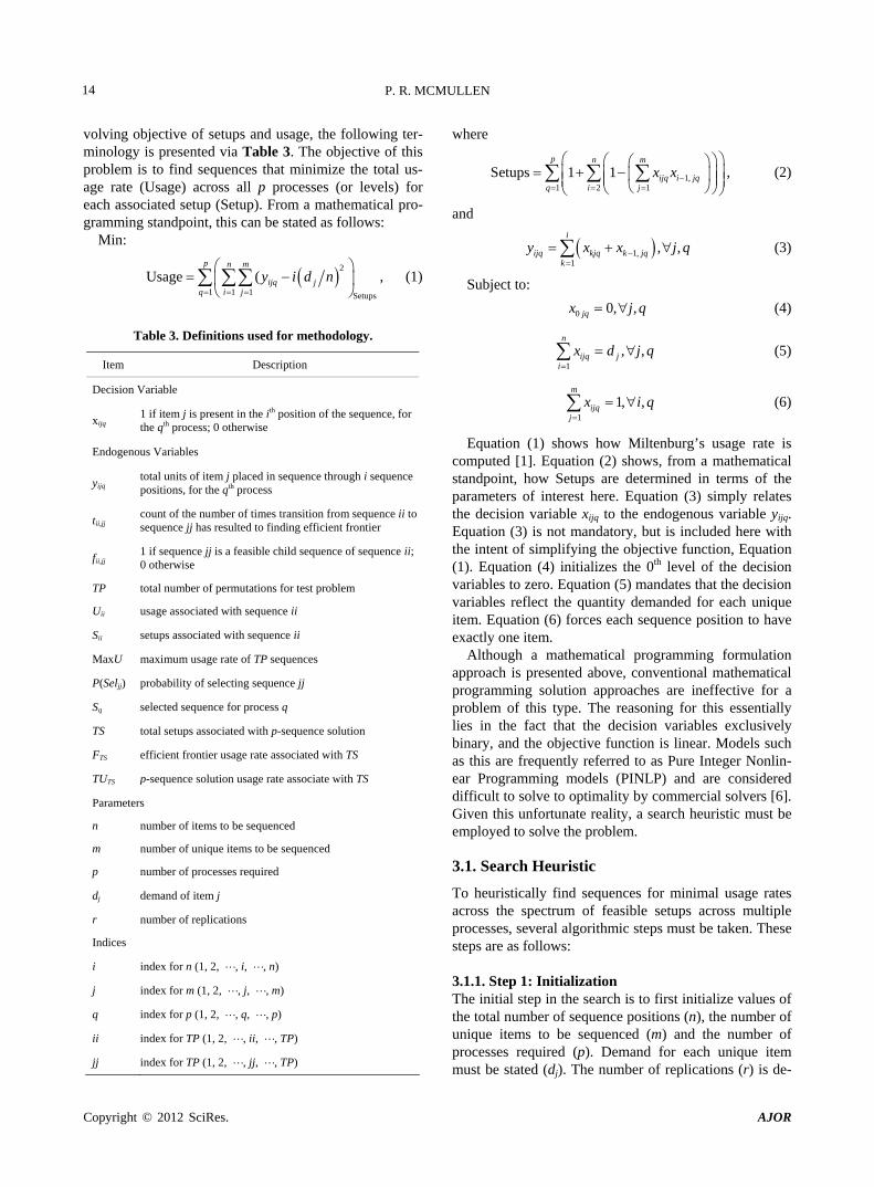
volving objective of setups and usage, the following ter-minology is presented via Table 3. The objective of this problem is to find sequences that minimize the total us-age rate (Usage) across all p processes (or levels) for each associated setup (Setup). From a mathematical pro-gramming standpoint, this can be stated as follows:

Min:

2

Setups

jd n

1 1 1

Usage (p n m

ijqq i j

y i

, (1)

Table 3. Definitions used for methodology.

Item Description

Decision Variable

xijq 1 if item j is present in the ith position of the sequence, for the qth process; 0 otherwise

Endogenous Variables

yijq total units of item j placed in sequence through i sequence positions, for the qth process

tii,jj count of the number of times transition from sequence ii to sequence jj has resulted to finding efficient frontier

fii,jj 1 if sequence jj is a feasible child sequence of sequence ii; 0 otherwise

TP total number of permutations for test problem

Uii usage associated with sequence ii

Sii setups associated with sequence ii

MaxU maximum usage rate of TP sequences

P(Seljj) probability of selecting sequence jj

Sq selected sequence for process q

TS total setups associated with p-sequence solution

FTS efficient frontier usage rate associated with TS

TUTS p-sequence solution usage rate associate with TS

Parameters

n number of items to be sequenced

m number of unique items to be sequenced

p number of processes required

dj demand of item j

r number of replications

Indices

i index for n (1, 2, , i, , n)

j index for m (1, 2, , j, , m)

where

1,1 2 1

Setups 1 1p n m

ijq i jqq i j

x x

1,1

, ,i

ijq kjq k jqk

y x x j q

0 0, ,jq

, (2)

and

(3)

Subject to:

x j q

q index for p (1, 2, , q, , p)

ii index for TP (1, 2, , ii, , TP)

jj index for TP (1, 2, , jj, , TP)

1

, ,n

ijq ji

(4)

x d j q

1

1, ,m

ijqj

(5)

x i q

(6)

Equation (1) shows how Miltenburg’s usage rate is computed [1]. Equation (2) shows, from a mathematical standpoint, how Setups are determined in terms of the parameters of interest here. Equation (3) simply relates the decision variable xijq to the endogenous variable yijq. Equation (3) is not mandatory, but is included here with the intent of simplifying the objective function, Equation (1). Equation (4) initializes the 0th level of the decision variables to zero. Equation (5) mandates that the decision variables reflect the quantity demanded for each unique item. Equation (6) forces each sequence position to have exactly one item.

Although a mathematical programming formulation approach is presented above, conventional mathematical programming solution approaches are ineffective for a problem of this type. The reasoning for this essentially lies in the fact that the decision variables exclusively binary, and the objective function is linear. Models such as this are frequently referred to as Pure Integer Nonlin-ear Programming models (PINLP) and are considered difficult to solve to optimality by commercial solvers [6]. Given this unfortunate reality, a search heuristic must be employed to solve the problem.

3.1. Search Heuristic

To heuristically find sequences for minimal usage rates across the spectrum of feasible setups across multiple processes, several algorithmic steps must be taken. These steps are as follows:

3.1.1. Step 1: Initialization The initial step in the search is to first initialize values of the total number of sequence positions (n), the number of unique items to be sequenced (m) and the number of processes required (p). Demand for each unique item must be stated (dj). The number of replications (r) is de-


P. R. MCMULLEN 15

termined. All permutations for the test problem are gen-erated—the number of permutations is set to TP, and each permutation is assigned an ID label. From these permutations, the pairwise relationships between all TP sequences are inspected. If sequence jj is a feasible child sequence of sequence ii, then the matrix value fii,jj is set to one. Otherwise, this value of fii,jj is set to zero. For all TP sequences, the usage (Uii) and setups (Sii) values are determined, along with the maximum usage (MaxU). Mathematically, Uii and Sii are as follows:

2

ji d n

1,2 1

n m

ij i ji j

b b

1 1

n m

ii iji j

U a (7)

1 1iiS , (8)

where aij represents the number of item j in the sequence through the ith position, and bij is one if item j is present in the ith sequence position, zero otherwise. Note that these two formulae are essentially the same as shown in Equations (1) and (2) respectively, with the difference being that these two formulae consider only one process, whereas the Equations (1) and (2) consider p processes. The parent sequence for the 0th level is always the trivial sequence—the sequence where all of the “As” are placed into the sequence, followed by the “Bs,” etc. It is noted that the permutation index values, values of Uii and Sii, and fii,jj values are shown for the example problem in Table 1.

3.1.2. Step 2: Candidate Sequence for Next Process The sequence that was selected for the last process is now given status as the parent sequence. The value of q is set to the appropriate level. Each of the candidate sequences is given a probability of selection via a probabilistic mechanism. This probabilistic mechanism is a function of the candidate’s usage rate (Ujj). Lower usage rates are more attractive, as the lowest usage rate for each unique setup across all processes describes the efficient frontier. The probability of selecting candidate sequence jj when sequence ii is the parent sequence is as follows:

,

,1

1 Ma

1 M

ii jj

jj TP

ii jjjj

P Sel

x

ax

jj

jj

f U U

f U U

, (9a)

If the researcher wishes to incorporate the concept of pheromone into the probability of selecting candidate sequence jj, P(Seljj) is calculated as follows:

This is similar to Equation (9a), with the difference being that (9b) incorporates the transition matrix, tii,jj into the calculation, which increases the probability of transi-tioning from sequences ii to jj, which have historically been observed to result in strong performance in terms of the efficient frontier.

It should be noted that infeasible child sequences of sequence ii are excluded from these calculations, as their associated fii,jj values are zero, forcing nonexistent prob-abilities.

3.1.3. Step 3: Selection of Next Sequence via Monte-Carlo Simulation

For all selection candidates, a cumulative probability distribution table is constructed, based upon the probabil-ity values determined via Equation (9a) or (9b). A ran-dom number on the [0, 1) interval is then generated and matched with the appropriate child sequence candidate. This appropriate child sequence candidate is now classi-fied as the selected sequence. The selected sequence for process q is noted as Sq.

3.1.4. Step 4: Iterate toward p Steps 1 and 2 are repeated for each of the p processes.

3.1.5. Step 5: Objective Function and Efficient Frontier

For each of the p sequences selected via the three prior steps, their values of setups (Sjj) and usage (Ujj) are de-termined and summed, and determine the total setups (TS) and corresponding total usage rate (TUTS) for the p-sequence solution.

3.1.6. Step 6: Efficient Frontier If the usage rate for the p-sequence solution (TUTS) is superior to that on the efficient frontier for the corre-sponding number of setups, than the p-sequence solution usage rate becomes part of the efficient frontier. In mathematical terms, this is as follows:

If TUTS < FTS, then FTS = TUTS (10)

If transition is used for seeking an optimal solution— that is, if Equation (9b) is used instead of Equation (9a), then the new efficient frontier results in the transition matrix being updated. Specifically, the values of the transition matrix that comprise the recent traversal/solution that resulted in the new efficient frontier value are incremented by one. This is done to reinforce, or en-courage traversal through sequences that show relative promise. Mathematically, this is as follows:

, ,

, ,1

1 M

1 M

ii jj ii jj

jj TP

ii jj ii jjjj

t fP Sel

t f

ax

ax

jj

jj

U U

U U

1 1, , 1, 2, ,q q q qS S S St t q p

(9b)

(11)

If transition is not used for seeking an optimal solution, Equation (11) is ignored.


P. R. MCMULLEN 16

3.1.7. Step 7: Iteration toward r Steps (1)-(5) are repeated r times. Again, r is a user- specified parameter which dictates the number of itera-tions, or replications.

3.1.8. Step 8: Report Findings At the end of the iterative process, the efficient frontier is reported, along with all information associated with per-formance.

3.2. Performance Measures

There are two performance measure of interest associated with this research effort. These performance measures are: relative inferiority to optimal; number of voids in the efficient frontier; and CPU time.

Relative Inferiority is the degree to which the search- based solution is “above,” or inferior to, the optimal so-lution. If (FO)S is used to note the optimal frontier usage for some number of setups, and (FS)S is used to note the frontier usage associated with the search heuristic (for the same number of setups) described above, then the Relative Inferiority (RI) can be computed as follows:

RI

1S mp

F F

np

np

S O OS S SF

mp (11)

It is, of course, desired that the relative inferiority be minimized. Figure 3 provides an illustration of relative inferiority for the example problem.

The second performance measure of interest here is the number of frontier voids. A frontier void is a measure of the heuristic’s failure to span the gamut of the efficient frontier. This particular concern is a widely acknowl-edged problem in the world of multiple objective opti-mization, where (as is the case here) the researcher at-tempts to minimize some objective function (usage) across a variety of conditions (setups). The number of frontier voids is easily determined, as it is the number of times that the search heuristic fails to find a solution on the efficient frontier, where an optimal solution is known to exist. Figure 4 details this via the example problem. Here, one will notice that there is a single frontier void when there are eleven opportunities for voids. This fron-tier void resides at (36) setups. The optimal solution shows that sets of sequences exist for as few as (30) set-ups, and as many as (40) setups (eleven total unique set-ups). This means that the search heuristic failed on one occasion to find a full set of solutions. This frontier void performance can then be “standardized” to one out of eleven, or 9.09%. In the interest of full disclosure, it is appropriate to note that the example shown in Figure 3 resulted in zero frontier voids (0.0%).

Figure 3. Relative inferiority of efficient frontier for exam-ple problem.

Figure 4. Illustration of single frontier void for example problem.

4. Experimentation

The methodology presented above is used on several test problem sets from the literature. These test problem sets contain items requiring sequencing, possessing varying degrees of item homogeneity. The five general problem sets are detailed on the Appendix. These problem sets are also used for a varying degree of processes (p)—all problems employ as few as two processes (p = 2), some employ as many as ten processes (p = 10). For each problem studied, the performance measures of relative inferiority, frontier voids and CPU time are determined and analyzed. The performance summary information is broken down into three categories. The first category is the search heuristic associated with not using transition, where the selection probability is governed by Equation (9a). The second category is the search heuristic associated with the use of transition, where the selection probability is governed by Equation (9b), and the transition matrix is updated via Equation (11). The third category is the result of a simulated annealing solution approach from a previous research effort. Each of these categories is hereafter referred to as search strategies. It is important to note that to make a fair comparison between these three strategies, each strategy exploited the same magnitude of search space. The magnitude of search space is dictated by the number of replications (r). In other words, the number of replications (r) was kept the same for each


P. R. MCMULLEN 17

strategy for each of the fifty-five unique problems.

4.1. Research Questions

To make a determination of which strategies perform best on the problem sets, the following research ques-tions are posed:

1) Does the strategy have an effect on relative inferior-ity? If so, which strategies are best? Do any of the strate-gies produce optimal results from the standpoint of sta-tistical significance?

2) Does the strategy have an effect on the degree of frontier voids? If so, which strategies are best? Do any of the strategies produce optimal results from the standpoint of statistical significance?

The first two parts of each of these research questions will be addressed via single-factor ANOVA and appro-priate pairwise comparison tests. The final part of each research question will be a single-sample t-test, with the following hypotheses:

H0: µ = 0

HA: µ > 0

Here, µ represents the population mean of the per-formance measure of interest (either relative inferiority or the frontier void ratio). The “0” represents optimality, either in the form of a relative inferiority of “0” or a frontier void ratio of “0”.

4.2. Computational Experience

The search heuristic described in the methodology sec-tion was coded using the Java Development Kit version 6, on the Microsoft Vista operating system with an AMD Turion 64 × 2 processor, having a CPU speed of 1.90 GHz. In all instances, efforts were made to maximize the computational efficiency of the algorithms.

5. Experimental Results

The research questions are first addressed, followed by a presentation of results for all problem sets and a discus-sion of CPU time.

5.1. Research Questions

For the first research question, it is clear that the strategy has an effect on relative inferiority performance (F = 43.73, p < 0.001). Means and standard deviations of rela-tive inferiority are presented in Table 4. From inspection of Table 4, it is clear that in terms of relative inferiority, the two search heuristics presented here outperform the Simulated Annealing approach from a prior research ef-fort. In fact, subsequent analysis shows that while the heuristic without transition does not statistically show optimality (mean inferiority of zero; t = 3.92, p = 0.0001),

the heuristic with transition does statistically show opti-mality (t = 1.21, p = 0.12).

For the second research question, it is also clear that the heuristic strategy has an effect on the performance measure of frontier void ratio (F = 2.33, p = 0.10). While this p-value is higher than the one associated with the first research question, Table 5 does show that the results associated with the heuristic presented with this research are desirable to those associated with the research effort that presented the Simulated Annealing approach [2]. For frontier void ratio, the heuristics presented in the meth-odology section are roughly half to magnitude from the earlier research effort. While the heuristic with transition enjoys a slight advantage in terms of relative inferiority, the heuristic without transition enjoys a slight advantage in terms of frontier void ratio.

5.2. Problem Set Results

Tables 6(a)-(e) show results in terms of relative inferior-ity and frontier void ratio for each of the three strategies. Each table is dedicated to a unique problem set. As the five problem sets and their results are inspected, it be-comes clear that the methodology presented with this research consistently outperforms the simulated anneal-ing methodology from an earlier research effort [2], es-sentially validating the results shown in Tables 4 and 5.

5.3. CPU Time

For each of the fifty-five problems studied, CPU time was captured for the two heuristics presented here. Space limitations prevent presenting them on a by-problem basis, but means are summarized here: the heuristic that does not employ transition results in a mean CPU time of 90.6 seconds, while the heuristic that does employ transition results in a mean CPU time of 91.2 seconds. This slight Table 4. Performance comparison of strategies for relative inferiority.

Strategy Mean Standard Deviation

Simulated Annealing 2.774% 2.880%

Heuristic without Transition 0.308% 0.582%

Heuristic with Transition 0.020% 0.121%

Table 5. Performance comparison of strategies for frontier void ratio.

Strategy Mean Standard Deviation

Simulated Annealing 2.787% 5.303%

Heuristic without Transition 1.282% 3.070%

Heuristic with Transition 1.389% 3.523%


P. R. MCMULLEN


18

Table 6. Results for problem. (a) set A0; (b) set A1; (c) set A2; (d) set A4; (e) set A5.

(a)

SA Without Transition With Transition Problem Processes

Inferiority Void % Inferiority Void % Inferiority Void %

B 2 4.76 0.00 0 0.00 0 0.00

B 3 4.81 0.00 0 0.00 0 0.00

B 4 4.35 0.00 0 0.00 0 0.00

B 5 3.87 0.00 0 0.00 0 0.00

B 6 3.47 0.00 0 0.00 0 0.00

B 7 3.12 0.00 0.42 0.00 0 0.00

B 8 3.39 0.00 0.65 0.00 0 0.00

B 9 3.62 0.00 1.05 0.00 0 0.00

B 10 4.41 0.00 1.52 0.00 0.21 0.00

Average 3.98 0.00 0.40 0.000 0.02 0.000

Std. Dev 0.62 0.00 0.56 0.000 0.07 0.000

(b)



B 2 0 0.00 0 0.00 0 0.00

B 3 0 0.00 0 0.00 0 0.00

B 4 0 0.00 0 0.00 0 0.00

C 2 2.32 0.00 0 0.00 0 0.00

C 3 4.31 0.00 0 0.00 0 0.00

C 4 5.7 0.00 0.64 0.00 0 0.00

Average 2.06 0.00 0.11 0.00 0.00 0.00

Std. Dev 2.49 0.00 0.26 0.00 0.00 0.00

(c)



B 2 0 0.00 0 0.00 0 0.00

B 3 0 0.00 0 0.00 0 0.00

B 4 0.09 0.00 0 0.00 0 0.00

Average 0.03 0.00 0.00 0.00 0.00 0.00

Std. Dev 0.05 0.00 0.00 0.00 0.00 0.00

(d)



B 2 0 0.00 0 0.00 0 0.00

B 3 0 0.00 0 0.00 0 0.00

B 4 0 0.00 0 0.00 0 0.00

B 5 0.45 0.00 0 0.00 0 0.00

P. R. MCMULLEN 19

Continued

B 6 0.29 0.00 0.09 0.00 0 0.00

C 2 3.34 0.00 0 0.00 0 0.00

C 3 6.21 0.00 0 0.00 0 0.00

C 4 5.35 0.00 0 0.00 0 0.00

C 5 4.54 0.00 1.4 0.00 0 0.00

D 2 13.19 12.50 0 0.00 0 0.00

D 3 9.46 8.33 0 0.00 0 0.00

D 4 7.24 6.25 0 0.00 0 0.00

E 2 8.54 12.50 0 0.00 0 0.00

E 3 8.03 8.33 0 0.00 0 0.00

E 4 3.82 12.50 0.87 6.25 0 0.00

F 2 1.59 22.22 0 0.00 0 0.00

F 3 1.58 15.38 0 7.69 0 7.69

F 4 0.95 11.76 1.05 11.76 0 11.76

Average 4.14 6.10 0.19 1.43 0.00 1.08

Std. Dev 3.94 7.05 0.43 3.43 0.00 3.22

(e)



B 2 0 0.00 0 0.00 0 0.00

B 3 0 0.00 0 0.00 0 0.00

B 4 0 0.00 0 0.00 0 0.00

B 5 1.86 0.00 0 0.00 0 0.00

B 6 1.72 0.00 0 0.00 0 0.00

B 7 1.59 0.00 0.73 0.00 0 0.00

B 8 1.46 0.00 0.85 0.00 0 0.00

B 9 1.35 0.00 2.2 0.00 0 0.00

C 2 4.64 0.00 0 0.00 0 0.00

C 3 4.79 0.00 0 0.00 0 0.00

C 4 3.6 0.00 0 0.00 0 0.00

C 5 3.07 0.00 0 0.00 0 13.33

C 6 2.54 0.00 0.4 5.56 0 11.11

C 7 3.15 0.00 2.18 4.76 0.88 9.52

D 2 0 14.29 0 0.00 0 0.00

D 3 0 10.00 0 10.00 0 10.00

D 4 0 7.69 0 7.69 0 7.69

D 5 0 6.25 1.65 6.25 0 0.00

D 6 0 5.26 1.22 10.53 0 5.26

B 2 0 0.00 0 0.00 0 0.00

Average 1.57 2.29 0.49 2.36 0.05 3.00

Std. Dev 1.66 4.28 0.77 3.78 0.20 4.76


P. R. MCMULLEN


20

difference in CPU time can be explained by the extra computation involving tii,jj in Equation (9b) as compared to (9a), along with the extra step required to update tii,jj associated with transition in Equation (11). CPU times for the simulated annealing approach are much less than the CPU times for the two heuristic approaches presented here. CPU times never exceeded 10 seconds for any problem.

6. Limitations and Opportunities

This research presented a general approach to address the multiple-process sequencing problem with the objectives of setups and usage rate. Results were found to be a sub-stantial improvement over an earlier effort involving simulated annealing. Despite this favorable outcome, there are some constraining issues that need mentioning.

6.1. Problem Breadth

The size of the problem is a constraining factor which dictates which problems can be solved to optimality. One will note that from Figure 1 that solving a problem to optimality is a cumbersome task—this even applies to very small problems. The problem shown in Figure 1 is essentially the smallest example imaginable, having just twelve unique permutations and only two levels. Never-theless, the solution space becomes large. For larger problems with more permutations and more levels re-quiring processing, this issue only becomes more severe. Given this combinatorial explosion, comparing heuristic solutions to optimal solutions is only available for smaller problems.

6.2. Permutation-Based Approach

Another constraining factor is specific to the heuristic approach presented. One will notice that Equations (9a) and (9b) involve feasibilities (fii,jj). Capturing values for each of these endogenous variables involves enumerating through each of the TP permutations TP times so that the binary values of fii,jj can be captured. This endeavor is computationally intensive, contributing O(TP2) to CPU time and memory requirements [7]. Even with high- speed computing, along with Java’s ability to allocate memory to the heap, the O(TP2) issue limits the size of the problem that can be solved via the presented heuristic. This problem only gets worse as the number of feasible permutations grows (as TP increases). It is important to note that the author attempted to avoid a component of the O(TP2) order, but omission of this element led to a relatively weak list of candidate solutions, and a subsequent marginal heuristic performance. As such, this research effort has sacrificed some computational efficiency so that a near-optimal performance could be

gained.

6.3. Buffer Size of One

As stated earlier, a pervasive assumption throughout this research is that there is a buffer size of one. This means that whenever re-sequencing is performed, an item can move forward in the sequence one position at most. It is possible to use buffer sizes of larger than one. If this were to be done, however, the breadth of the problem would increase (as there would be more feasible “re- sequences” because items would be permitted to move up more than one sequence position), further increasing computational efforts to find optimal or near-optimal solutions.

6.4. Future Research Opportunities

The limiting factors listed above, in one form or another, essentially all pertain to problem size and the difficulty of finding optimal solutions and/or good-quality heuris-tic-based solutions via a reasonable computational effort. Such limiting factors, of course, also present opportuni-ties for subsequent research.

A salient opportunity for future research relates to finding a strong list of candidate solutions while by- passing the feasibility matrix (the values of fii,jj). When this happens, CPU performance will improve, along with reduced memory requirements, enabling the researcher to address problems of a larger size.

Another opportunity for future research applies to us-ing a buffer-size of something larger than one. This, of course, is more computationally expensive, but with gains in computational resources, coupled with the point immediately above, this issue could be explored as well.

Yet another research opportunity relates to finding near-optimal solutions to these problems via exploitation of some of the other search heuristics (such as genetic algorithms [8], tabu search [9], etc.) that repeatedly show promise.

REFERENCES [1] J. Miltenburg, “Level Schedules for Mixed-Model As-

sembly Lines in Just in Time Production Systems,” Management Science, Vol. 35, No. 2, 1989, pp. 192-207. doi:10.1287/mnsc.35.2.192

[2] P. R. McMullen, “Limited Re-Sequencing for Mixed Models with Multiple Objectives,” American Journal of Operations Research, Vol. 1, No. 4, 2011, pp. 220-228.

[3] M. Dorigo and L. M. Gambardella, “Ant Colonies for the Traveling Salesman Problem,” Biosystem, Vol. 43, No. 1, 1997, pp. 73-81. doi:10.1016/S0303-2647(97)01708-5

[4] M. Lahmar and S. Banjaafar, “Sequencing with Limited Flexibility,” IIE Transactions, Vol. 39, No. 10, 2007, pp. 937-955. doi:10.1080/07408170701416665

http://dx.doi.org/10.1287/mnsc.35.2.192

http://dx.doi.org/10.1016/S0303-2647(97)01708-5

http://dx.doi.org/10.1080/07408170701416665

P. R. MCMULLEN 21

[5] M. Masin and Y. Bukchin, “Diversity Maximization Approach for Multiobjective Optimization,” Operations Research, Vol. 56, No. 2, 2008, pp. 411-424. doi:10.1287/opre.1070.0413

[6] L. A. Schrage, “LINGO: The Modeling Language and Optimizer,” Lindo Systems, Inc., Chicago, 2006.

[7] R. Sedgewick, “Algorithms in Java: Third Edition,” Ad-dison-Wesley, Boston, 2003.

[8] J. H. Holland, “Adaptation in Natural and Artificial Systems,” First Edition, University of Michigan Press, Ann Arbor, 1975.

[9] F. Glover, “Tabu Search: A Tutorial,” Interfaces, Vol. 20,

No. 1, 1990, pp. 74-94. doi:10.1287/inte.20.4.74

[10] P. R. McMullen, “An Ant Colony Optimization Approach to Addressing a JIT Sequencing Problem with Multiple Objectives,” Artificial Intelligence in Engineering, Vol. 15, No. 3, 2001, pp. 309-317. doi:10.1016/S0954-1810(01)00004-8

[11] P. R. McMullen, “A Kohonen Self-Organizing Map Ap-proach to Addressing a Multiple Objective, Mixed Model JIT Sequencing Problem,” International Journal of Pro-duction Economics, Vol. 72, No. 1, 2001, pp. 59-71. doi:10.1016/S0925-5273(00)00091-8

Appendix: Problem Sets

The Appendix containing the problem set details used for this research. These problems were taken from the work of McMullen [10,11].

Problem set A0

Problem Item A Item B Item C Permutations

B 2 1 1 12

Problem set A1

Problem Item A Item B Item C Item D Item E Permutations

B 6 1 1 1 1 5040

C 5 2 1 1 1 15,120

Problem set A2

Problem Item A Item B Item C Item D Item E Permutations

B 8 1 1 1 1 11,880

Problem set A4

Problem Item A Item B Item C Item D Permutations

B 5 1 1 1 336

C 4 2 1 1 840

D 3 3 1 1 1120

E 3 2 2 1 1680

F 2 2 2 2 2520

Problem set A5

Problem Item A Item B Item C Permutations

B 4 1 1 30

C 3 2 1 60

D 2 2 2 90


http://dx.doi.org/10.1287/opre.1070.0413

http://dx.doi.org/10.1287/inte.20.4.74

http://dx.doi.org/10.1016/S0954-1810(01)00004-8

http://dx.doi.org/10.1016/S0925-5273(00)00091-8

Limited Re-Sequencing for Mixed-Models with Multiple...

Documents

Transcript of Limited Re-Sequencing for Mixed-Models with Multiple...