Like Father, Like Son?

The Effect of Political Dynasties on Economic Development∗

Siddharth Eapen George

20 November 2019

Please click here for latest version

Abstract

This paper studies how dynastic politics affects economic development in India, using variation from three distinct

natural experiments. We build a political agency model with overlapping generations to show that dynastic politics has

theoretically ambiguous economic effects: bequest motives may lengthen politicians’ time horizons (founder effects),

but heritable political capital makes elections less effective at holding dynastic heirs accountable (descendant effects).

We compile data on the family ties of all Indian legislators since 1947, and present three empirical findings. First, we

identify descendant effects using a close elections regression discontinuity design, and find that descendants worsen

poverty and public good provision in villages they represent. We develop a method to improve the external validity of

our RD estimates, and find that even non-marginal descendants perform poorly in office. Descendants underperform

partly due to moral hazard: they inherit voters loyal to their family, which dampens their performance incentives.

Second, we estimate founder effects by examining constituency boundary changes, and find that founders have positive

effects on economic development. Bequest motives influence founder behaviour: politicians with a son are twice as

likely to establish a dynasty and exert more effort while in office. Third, we identify the overall effects of dynastic

politics using an IV strategy based on the gender composition of past incumbents’ children. Dynastic politics generates

a “reversal of fortune” development pattern, where places develop faster in the short run (because of positive founder

effects), but are poorer in the long run (because negative descendant effects outweigh positive founder effects).

∗Siddharth Eapen George, siddharthgeorge@fas.harvard.edu, Harvard University, Cambridge, MA, USA. I am indebted to my advisors Rohini Pande,Michael Kremer, Abhijit Banerjee and Emily Breza for advice and encouragement. I thank Sreevidya Gowda, Anjali R and Zubayer Rahman for researchassistance. I am grateful to Alberto Alesina, Tim Besley, Kirill Borusyak, Laurent Bouton, Moya Chin, Cesi Cruz, Jishnu Das, Oliver Hart, AbrahamHolland, Asim Khwaja, Gabriel Kreindler, Asad Liaqat, Eric Maskin, Nathan Nunn, Dev Patel, Tzachi Raz, Henrik Sigstad, Daniel Smith, ArvindSubramanian, Edoardo Teso, Sophie Wang and Chenzi Xu for helpful conversations. This paper also benefitted from comments during seminars atHarvard, MIT, Mannheim, the World Bank and at the MPSA, APSA, NEUDC and EBE conferences. Siddharth gratefully acknowledges financial supportfrom LEAP, the Warburg Fund and the IGC State Capacity Programme.

1

1 Introduction

Over the past two centuries, many societies democratised in part to end hereditary rule. Yet political dy-

nasties remain ubiquitous in democratic countries: nearly 50% have elected multiple heads of state from

a single family, and 15% are currently led by the descendant of a former leader.1 Politics is significantly

more dynastic than other occupations in democratic societies. Individuals are, on average, five times more

likely to enter an occupation their father was in. But having a politician father raises one’s odds of entering

politics by 110 times, more than double the dynastic bias of other elite occupations like medicine and law.2

Despite their prevalence and influence, we know little about the economic effects of political dynasties.

Economic theory makes ambiguous predictions about how dynastic politics affects development. On

the one hand, the incentive to establish a dynasty might lengthen the time horizons of (often short-termist)

politicians and encourage them to make long-term investments. These bequest motives, which we call

founder effects, could be good for economic development. On the other hand, if some political capital is heri-

table (such as a prominent name or a powerful network), dynastic politics can render elections less effective

at selecting good leaders and disciplining them in office. We refer to the (typically negative) selection and

incentive consequences of inheriting political capital as descendant effects. The overall impact of dynastic

politics is ambiguous, because it is the net result of founder and descendant effects.3

We study the economic impacts of dynastic politics in India, where legislators play a significant role in

local economic development, and the merits of dynasties are publicly contested.4 Research on dynasties is

often stymied by limited data on politicians’ family ties. To overcome this challenge, we compile detailed

biographical information on (i) all members of India’s national parliament (MPs) since 1862, when Indians

were first allowed to serve in the British-era legislative assemblies; and (ii) on the universe of candidates

(over 105,000) in state and national parliament elections since 2003. We document that political dynasties

1We identify democratic countries using the Economist Intelligence Unit’s and Freedom House’s classification.2We produce these statistics using census microdata from the universe of democratic countries that list “legislator” or “legislative

activities” as a separate occupational category. Details are in Section 3.1. The occupation of “Economist” is also highly dynastic:having an economist father increases one’s probability of being an economist by 63 times.

3The direction of founder and descendant effects are both uncertain. Founder effects could be bad for development if bequestmotives encourage parents to make private investments in their political capital (say, by targeting private goods to build a loyal votebase) rather than provide public goods that are valued by all voters. Descendant effects could be positive if the human capital thatdescendants inherit (like knowledge of how to govern) outweigh the negative selection and incentive consequences of inheritingpolitical capital. We will use two different identification strategies to separately identify founder and descendant effects.

4These two quotes by Indian politicians illustrates the contentious nature of dynastic politics. Sukhbir Singh Badal, a dynasticpolitician, argues that reputational concerns motivate political families to perform better than new entrants. By contrast, VenkaiahNaidu, who recently defeated Mahatma Gandhi’s grandson to become India’s Vice President, thinks that the returns to politicalfamilies are mostly private.

“This family system runs because of credibility. Why do people want to buy a BMW...You come out with a new car...nobody will buy it.” (Sukhbir Badal, dynasticpolitician)

”Dynasty in democracy is nasty but it is tasty to some people. That is a weakness of our system.” (Venkaiah Naidu, defeated Mahatma Gandhi’s grandson to becomecurrent VP)

2

are widespread in India: 10% of MPs are children of former MPs, which is nearly 2500 times higher than

random chance would predict. We compile maps of historical constituency boundaries and spatially link

villages with the set of parliamentary constituencies they have resided in since Indian independence in

1947. During this period, over 35% of villages have been represented in the national parliament by at least

one dynastic politician.

We employ three different empirical strategies to identify (i) descendant effects, (ii) founder effects, and

(iii) the overall impact of a dynastic political environment on economic development. First, we identify

descendant effects using a close elections regression discontinuity (RD) design. We focus on close races be-

tween dynastic descendants (ie. direct relatives of former officeholders) and non-dynasts, and we compare

places where a descendant narrowly won to those where a descendant narrowly lost.5 In these elections,

descendants and non-dynasts have similar demographic and political characteristics, and win in similar

places and at similar rates. Nevertheless, we find negative economic effects when a descendant narrowly

wins. Villages represented by a descendant have lower asset ownership and public good provision after

an electoral term: households are less likely to live in a brick house and to own basic amenities like a re-

frigerator, mobile phone, or vehicle. Moreover, voters assess descendants to perform worse in office. An

additional standard deviation of exposure to descendants lowers a village’s wealth rank by 12pp.

One potential external validity concern with our RD results is that they are identified based on descen-

dants in marginal races. These descendants — who are in close races despite the political capital they inherit

— may be particularly weak. We develop a method to estimate the treatment effect of an “average” (rather

than marginal) descendant, and show that our conclusions continue to hold. We use the fact that aggregate

forces which affect a party’s overall popularity in an election result in shocks to each descendant’s win mar-

gin (ie. the running variable in the RD). We find that descendants in close races despite their party having a

good year perform particularly poorly in office. By contrast, descendants in close races when their party is

having a bad year perform less poorly in office, though still worse than the average non-dynast. We use this

variation to estimate the effect of politicians whose victory margin, absent aggregate party swing, would

have been similar to that of the average descendant (which is 10%). We find that average descendants

perform much better than marginal descendants, but still have negative effects on development relative to

non-dynasts. This approach could potentially also be used to improve external validity of RD estimates in

other settings where there are shocks to the running variable.

We provide evidence that moral hazard is one reason that descendants underperform. Descendants

5 The sample includes all state and national elections since 2003 where the top two candidates are a dynastic descendant and anon-dynast (or vice versa).

3

face moral hazard because they inherit (some) voters loyal to their predecessor (usually father)6, and this

dampens incentives to exert effort and perform well in office. Indeed, a significant fraction of political

capital appears to be heritable: the parent-child vote share correlation is 0.23, about one-third as large as

the correlation between a politician’s own vote shares in different elections. We isolate the effects of moral

hazard on performance using constituency boundary changes, which affect the overlap between a descen-

dant’s electoral district and her predecessor’s former electoral district. Redistricting provides a shock to

the number of votes a descendant inherits each election. The same descendant earns 1.2pp more votes and

completes 2.8pp fewer projects when redistricting increases the spatial overlap between her constituency

and her father’s former constituency by 10%. Overall, moral hazard explains about 40% of the performance

gap between descendants and non-dynasts.

We argue that part of the remaining performance gap is due to dynastic descendants being negatively

selected relative to other politicians. Among dynastic descendants, sons-in-law perform significantly better

than sons, echoing findings from the family firms literature that hired professional managers are more

competent than family CEOs (Bennedsen et al. 2007; Bertrand and Schoar 2006). Moreover, sons with

brothers perform better than only sons, hinting at the benefits of a larger selection pool.

Second, we show that the incentives to establish a dynasty motivate politicians to perform better in

office. Isolating founder effects is challenging because most descendants run for office in their father’s con-

stituency. Redistricting results in some villages that were represented by the founder being moved into a

neighbouring constituency before the descendant enters politics. These villages are thus never represented

by a descendant; they are currently in a non-dynast’s constituency but were represented in the past by a

founder. Comparing villages in the same present-day constituency, we find that villages previously rep-

resented by founders are wealthier and have more public goods. Redistricted villages are not selectively

chosen (they have similar characteristics to villages that remained in their original constituency), and redis-

tricting has no direct effect on development outcomes. These placebo tests increase our confidence that this

identification strategy captures the effect of exposure to founders. Overall, an additional standard deviation

of exposure to founders raises a village’s wealth percentile rank by 1.5pp.

We argue that the positive effects of founders are partly driven by bequest motives. To test whether

bequest motives affect in-office behaviour, we identify a shock to politicians’ time horizons based on the

gender composition of their children. Women face significant barriers to enter politics in India (only 9% of

candidates are women). As a result, conditional on the number of children, politicians who have a son are

twice as likely to found a dynasty (relative to politicians with only daughters), even though they appear6Most dynastic predecessors are fathers, though a small fraction are mothers, in-laws and spouses.

4

similar on most demographic and political characteristics. We show that politicians with a son exert more

effort while in office: they are 2pp more likely to complete local development projects (even conditional

on the same implementing agency), 6pp more likely to hold the stipulated quarterly meeting with local

bureaucrats to take stock of constituency development work, and are assessed by voters to perform better

in office.

Third, we estimate the overall effect of a (local) dynastic political environment, which is the net result of

founder and descendant effects. Our empirical strategy attempts to simulate the ideal experiment of going

from a world where dynasties are not possible (a non-dynastic local political environment) to a world where

they are possible (a dynastic local political environment). Because politicians with a son are more likely to

found dynasties, and sons typically run in their parents’ constituency, places where past incumbents had a

son are more exposed to both founders and descendants. Using this variation, we find that dynastic rule

has overall negative economic effects and results in a distinct “reversal of fortune” development pattern.

Exposure to MPs with a son initially has positive effects on development, when the first generation of politi-

cians is in power, due to bequest concerns. But these places — with greater early exposure to MPs with a

son — fall so far behind once the second generation of politicians enter politics and inherit their parents’

constituencies, that by the end of our sample period, they are poorer and have fewer public goods. These

time-varying patterns are consistent with the lifecycle of a dynasty, but inconsistent with the most obvious

confounding explanations (eg. son preference or other unobserved differences between politicians with a

son and those with only daughters). Moreover, both the initial positive effect and the subsequent negative

effect are absent in strongholds of parties with norms against dynasties, like the Communist parties. Over-

all, a standard deviation increase in exposure to dynastic rule lowers a village’s wealth percentile rank by

7pp.

We propose a simple theory of dynastic politics that is consistent with these three empirical facts. The

setup is a political agency model with electoral uncertainty, which we embed in an overlapping generations

framework. The key element of the theory is that both human capital and political capital are heritable.7

While in office, politicians exert costly effort to deliver public goods, and these costs are lower for competent

politicians. Fixed costs of entering politics lead to positive selection of citizens into politics. Parents receive

warm-glow benefits when their descendants hold political office, which creates signalling incentives for

parents to perform well in office and signal that they — and by extension, their descendants — are high-

types. If political entry costs are higher for women, politicians with a son will be more likely to have

7Human capital refers to skills that help a politician govern well, while political capital refers to assets (like name recognition) thathelp a politician get elected but do not improve in-office performance.

5

bequest motives. As a by-product of being in power, incumbents also acquire political capital that gives

them an electoral advantage. If some of this political capital is heritable, descendants will enter politics

at a lower threshold quality and face dampened performance incentives because they inherit votes from

their predecessor. This inherited political capital allows descendants to persist in power even when they

underperform. This simple theory explains our three main empirical facts — that (i) fathers are good for

development (because of bequest motives), (ii) sons are bad for development (because of negative selection

and moral hazard) and (iii) sons persist in power despite underperforming (because some political capital

is heritable).

Our paper extends the political economy of development literature in several ways. First, it contributes

to a small literature on political dynasties, summarised recently by Geys (2017), which documents the pri-

vate returns from family networks in politics (Smith 2012; Querubin 2015, 2013). Dal Bó, Dal Bó and Snyder

(2009) documents that marginal winners of US House races are more likely to have family members subse-

quently hold political office, and Cruz, Labonne and Querubin (2017) describe the advantages that family

networks confer during elections. Several papers study the consequences of dynastic rule. Besley and

Reynal-Querol (2017) show that hereditary rulers (like monarchs) can be motivated by career concerns to

perform well while in office. Asako et al. (2015), Tantri and Thota (2018), Dar (2018) and Bragança, Ferraz

and Rios (2015) all study the impacts of marginal dynastic descendants on short-run measures of economic

performance, usually finding negative effects. Our contribution is to separately identify founder and de-

scendant effects as well as to consider the overall effect of a dynastic political environment in a unified

theoretical framework and empirical setting. We also examine mechanisms for founder and descendant

behaviour, and attempt to deal with the external validity critique of descendants in close races.

Second, our paper is connected to a broader literature studying inefficiencies in collective choice. This

mostly theoretical literature documents the role of strategic voting (Austen-Smith and Banks 1996), infor-

mation frictions (Feddersen and Pesendorfer 1997; Pande 2011) and partisan bias (Krishna and Morgan

2011). It also highlights how political institutions, such as electoral rules (Dasgupta and Maskin 2008) and

term limits (Besley and Case 1995), can be designed to improve electoral accountability. We contribute to

this literature by showing how elections can deliver socially inefficient outcomes when political capital is

heritable.

Third, our results relate to papers in development economics that document “reversals of fortune” due

to institutions that concentrate political power. Acemoglu, Johnson and Robinson (2002) document a “re-

versal of fortune” due to colonisers setting up extractive institutions in places blessed with favourable

6

geography. Banerjee and Iyer (2005) document a similar pattern in India from landlords being vested with

political and revenue extraction power. We study the economic effects of an unusually common “bad” in-

stitution — dynastic politics — that has received relatively little empirical attention. Dynastic politics leads

to reversals of fortune because areas “blessed” with a politician who has a son initially fare better (since

that politician has bequest concerns) but eventually do worse when the descendant enters politics.

Finally, our paper finds similar stylised facts to the literature on family firms, which documents that

they are worse managed (Bloom and Van Reenen 2007; Lemos and Scur 2018; Bennedsen et al. 2007) and

examines theoretical reasons why (Burkart, Panunzi and Shleifer 2003). The family firms literature typically

argues that dynastic descendant CEOs underperform due to negative selection. By constrast, we show

that moral hazard is an important reason why descendants underperform. Moreover, the mechanisms

for persistence of business and political dynasties are theoretically distinct: founder CEOs typically have

control rights over their firm, while dynastic politicians have no formal power over voters.

The remainder of the paper is organised as follows. Section 2 proposes a simple theory of dynastic

politics. Section 3 describes the Indian context and the data we use. Section 4 presents results on descen-

dants effects. Section 5 presents results on founder effects. Section 6 presents results on the overall effect of

dynastic politics. Section 7 concludes.

2 A simple theory of dynastic politics

In this section, we develop a simple model to analyse the economic effects of dynastic politics. The setup

is based on the political agency framework used extensively by Besley (2007). We extend this model by

(i) introducing electoral uncertainty as in a probabilistic voting model and (ii) nesting it in an overlapping

generations (OLG) framework. The key element of the model is that both human capital and political capital

are heritable. Human capital refers to skills that enable a politician to govern well; an alternative term in

our context is “governing capital”. Political capital refers to assets (like name recognition or a powerful

network) that help a politician get elected, but do not improve in-office performance; an alternative term

might be “campaign capital”. Incumbents take costly actions to provide public goods, and these actions are

less costly for competent politicians, creating signalling incentives for founders. Parents receive warm-glow

benefits when their offspring hold political office. Heritable human capital thus gives incumbent parents

further incentive to perform well to signal to voters that they — and, by extension, their descendant —

are high types. However, incumbents also accumulate political capital while in office. When some of this

political capital (eg. a prominent name or a powerful network) is heritable, descendants can persist in

7

power even when they underperform.

2.1 The environment

Citizens An economy consists of a mass 1 of citizens. There are 2 generations, and each lives for 2 periods.

At birth, each citizen is assigned a type i = {q, j} that consists of (i) her ability level q ∼ U (0, 1) and (ii) a

parameter capturing her gender j ∈ {m, f }, where both occur with equal probability.

Politicians Each period, citizens elect a politician whose job is to provide a public good B ∈ {0, 1}. Politi-

cians are drawn from the citizenry. Each period, two citizens are randomly nominated to run for office and

pay entry cost φj > 0 if they contest the election. Women face significant barriers to entering politics in

many democratic societies, and we capture this by supposing φ f > φm.

Voting As in a standard probabilistic voting model, there are two sources of electoral uncertainty: (i) each

voter receives an idiosyncratic shock σi ∼ U[− 1

2 , 12

]and (ii) the incumbent receives an aggregate popu-

larity shock δ which determines the election. δ follows a general distribution function f that is unimodal,

non-uniform and symmetric around 0. Additionally, each period the incumbent acquires political capital

(eg. name recognition, control over the party machine) that delivers a share of k loyal votes in the next

election.8

Policymaking Incumbents receive benefits E, which capture the pecuniary and ego benefits from holding

public office, regardless of whether they deliver the public good. While in office, the incumbent chooses

effort e ∈ {0, 1} and delivers public good benefits B to citizens if and only if she exerts effort. Delivering

the public good is particularly challenging for less competent politicians. Hence, effort costs are ctq , where

ct ∼ U [0, C] varies based on the administrative and political complexity of delivering the public good in

period t.

Intergenerational Issues Each citizen has 1 offspring, whose ability is private knowledge to the offspring

and her parent. A parent receives warm-glow utility ψE (where ψ < 1) if her descendant holds political

office. Both human capital (ie. ability) and political capital are heritable but mean revert. Hence, a politician

with ability q has a descendant of expected ability qD = ρ(

q− 12

)+ 1

2 , ρ ∈ (0, 1). Similarly, an incumbent

8This assumption could be micro-founded in several ways. For example, suppose a fraction k voters are inattentive each period,and choose the candidate whose name they have heard before.

8

with political capital k passes on αk (where α < 1) to her descendant. All citizens have discount factor

β < 1.

Timing The timing of the model in each generation is as follows.

1. Generation t is born and nature assigns each citizen a type i = {q, j}.

2. Two citizens are randomly nominated to run for office and decide whether to pay φj and contest the

election. If a citizen declines, another is randomly nominated to run.

3. The shocks σi and δ are realised, and voting occurs.

4. The period 1 incumbent receives a draw from effort cost distribution c1 and chooses effort e1

5. Voters observe their payoffs, receive σi and δ, and decide whether to re-elect the incumbent or elect

the challenger

6. Generation t + 1 is born and parents observe their type i = {q, j}

7. The period 2 incumbent receives a draw from c2 and chooses e2

8. Payoffs are realised and the game ends.

2.2 Equilibrium

We characterise Perfect Bayesian Equilibria where politicians’ strategies are optimal given citizens’ beliefs

(and vice versa).

Voters Consider voters’ decision whether to re-elect an incumbent based on observing B1. Competent

politicians are more likely to deliver the public good in period 2, so voters maximise payoffs by inferring

incumbent type from B1.

If B1 = 0, voter i chooses to re-elect the incumbent over a fresh challenger iff EUincumbent = 0 + σi + δ >

qpB = EUchallengerr , where qp denotes the average ability of a fresh politician. Swing voters choose the in-

cumbent with probability 12 + δ− qpB. However, since the incumbent has also acquired political capital that

gives her a vote share advantage of k, her total vote share is VIncumbent = k + (1− k)(

12 + δ− qpB

), and she

gets re-elected with Pr (win|B1 = 0) = Pr(

VI >12

)= Pr

(δ > − k

2(1−k) + qpB)= 1− F

(− k

2(1−k) + qpB)

.

By contrast, if B1 = 1, then voters’ posterior belief that the incumbent is competent is q′p =

qp

qp+(1−qp)λ1>

qpwhere λ1 < 1 is the probability that the average politician would deliver the public good in period 1.

9

Hence, swing voter i chooses to re-elect the incumbent iff q′pB + σi + δ > qpB. By similar reasoning as

above, we obtain Pr (win|B1 = 1) = 1− F(− k

2(1−k) − B4qp

), where4qp = q

′p − qp.

In-office behaviour Absent bequest motives, the incumbent would always choose e = 0 in period 2. How-

ever, she can be motivated by re-election concerns to exert effort in period 1. In particular, the incumbent

chooses e1 = 1 iff c1 < (π1 − π0) · qβE, where πe denotes the incumbent is re-elected when she chooses

effort e. Observe that

π1 − π0 = Pr (win|e1 = 1)−Pr (win|e1 = 0) = F(− k

2 (1− k)+ qpB

)− F

[− k

2 (1− k)− B

(q′p − qp

)]

Hence, we can define λBS1 ≡ Pr (e1 = 1 |q) = (π1−π0)βEq

C to be an index of incumbent discipline in period 1

under the baseline model.

Entry A citizen of ability q derives expected time discounted value from office V (q) = E+λ1

(βπ1E− c1

q

)+

(1− λ1)π0βE. It can be shown that ∂V∂q = ∂λ1

∂q

(4πβE− c1

q

)+ λ1 · c1

q2 > 0. This condition says that the re-

turns to political office are increasing in ability, which is driven by fixed entry costs and effort costs that are

decreasing in ability. We can thus define q∗ to be the cutoff point at which V (q∗) = φ. Only citizens with

q > q∗ will find it optimal to enter politics. This positive selection of citizens into politics is consistent with

recent empirical evidence from Sweden (Dal Bó et al. 2017).

Two other points are noteworthy. First, higher barriers to entry for women result in q∗f > q∗m . Since

women and men are drawn from the same ability distributions, women will be less likely to enter politics

than men. Second, because some political capital is heritable, descendants of former incumbents start with

a αk electoral advantage. Hence, fixing a performance level B, dynastic descendants will be more likely to

win (ie. πD1 > π1 and πD

0 > π0). As a result, for any level of ability q, it will be the case that dynastic

descendants derive higher returns from political office VD (q) > V (q). The implication is that q∗D < q∗, ie.

that descendants have a lower quality threshold at which they enter politics.

2.2.1 Prediction #1: Politicians with sons perform better in office

Bequest motives Recall that the incumbent parent observes her descendant’s type — gender and ability

— after being elected but before choosing her effort level. Hence, before choosing her effort level, the

incumbent knows whether her descendant’s ability qD is sufficiently high to enter politics. If qD < q∗D, then

the incumbent always chooses e2 = 0. However, if qD > q∗D, then the incumbent internalises that delivering

10

the public good can raise her offspring’s chances of winning. This is because ability is heritable: voters will

(rationally) infer the descendant’s type from the parent’s performance.

Let qavgD =

q∗D+12 denote the average quality of a descendant politician. However, on observing that the

parent delivered B1 = B2 = 1, voters will update their beliefs about the parent, and consider her now to

have ability q′=

qp

qp+(1−qp)λ1λDP2

. Since ability is heritable, voters will also thus update upwards about the

descendants, and think she has ability q′D = ρ

(q′ − 1

2

)+ 1

2 > qavgD .

Hence, by choosing e2 = 1, the parent boosts her offspring’s descendant’s chance of winning by 4qD ·(∂Pr(D wins)

∂qD

)= (B4qD) · f

[B(qp − qD

)− αk

2(1−αk)

]. As a result, the period 2 incumbent chooses e2 = 1 if

c2 < B · f[

B(πp − πD

)− αk

2(1−αk)

]· ψE, which occurs with probability λDP

2 =B· f[

B(qp−qD)− αk2(1−αk)

]·ψE

C > 0.

How gender of politicians’ children affects voter welfare Consider an incumbent parent of ability q. The

expected ability level of her son or daughter is the same regardless of gender. However, since φ f > φm (ie.

women face greater barriers to enter politics), we have q∗f > q∗m, so a daughter is less likely to be above the

entry threshold than a son. Politicians with a son should thus be more affected by bequest motives. Since a

politician always shirks in period 2 when not motivated by bequest concerns, we should expect politicians

with a son to deliver more public goods than incumbents who have only daughters.

Moreover, bequest motives make incompetent incumbents weakly more disciplined even in period 1.

Without bequest motives, incumbents choose e1 = 1 if c1 < (π1 − π0) βEq. But anticipating the possibility

of bequest motives, the period 1 incumbent chooses e1 = 1 if c1 < 124πβEq + 1

2 (4π) βEV (c2), where

V (c2) = max {E, E− c2 + ψE} .

Bequest motives thus strictly improve the welfare of older generation voters, since the incumbent is

strictly more likely to provide the public good in period 2 and weakly more likely to do so in period 1.

Hence, empirically we should expect older generation voters to be better off under politicians who have a

son.

Discussion In this model, politicians can only take actions to improve voter welfare. Moreover, political

capital is accumulated mechanically (eg. a fraction k voters are inattentive every period and vote for the

candidate whose name they recognise). Politicians cannot invest in political capital, say, by targeting pri-

vate goods to build a base for their descendant. Extending the model to include a richer action space for

politicians would make founder effects ambiguous. Politicians with a son would still be more motivated

by bequest concerns, but it would be ambiguous whether that motivates them to provide public goods and

build a reputation for delivering development, or provide private goods to a subset of voters and build a

11

reputation for clientelism9.

2.2.2 Prediction #2: Descendants underperform in office

Recall that dynastic descendants enter politics so long as qD > q∗D where q∗D < q∗. Rational voters realise

that descendants are on average worse types, but nonetheless a descendant is more likely to win in equilib-

rium if inherited political advantages αk are sufficiently large. Specifically, descendants are more likely to

win in equilibrium if 1− F[

B(πp − πD

)− αk

2(1−αk)

]> 1

2 ⇐⇒ αk >2B[πp−πD]

1+2B[πp−πD].

Having argued that the incentive to establish a political dynasty motivates potential founders to perform

better for older generation voters, we now study how descendants perform for younger generation voters.

We first consider the performance of non-dynasts as a benchmark. Younger generation voters’ expected util-

ity (in periods 3 and 4) from electing a non-dynast is EU = B[qp + λ1

(1− qp

)]+ βB

[qp +

(1− qp

)(1− λ1) qp

],

where qp is the quality of the average politician. The first term captures period 3 expected utility and the

second term captures discounted period 4 expected utility.

Worse selection As discussed above, fixed entry costs result in positive selection of citizens into politics,

ie. qp > 12 . But dynastic descendants are on average worse types than the average politician qavg

D < qp .

Since ∂EU∂q > 0, we should expect descendants to perform better than non-dynasts because they are better

selected.

Moral hazard Moreover, because descendants inherit political capital that is unrelated to their perfor-

mance (eg. name recognition), descendants have weaker performance incentives than non-dynasts. Recall

that an incumbent earns private political capital k while in office and thus exerts effort with probability

λBS1 = 4Pr(re−elected)·βE

C =βE·{

F(− k

2(1−k)+qpB)−F[− k

2(1−k)−B(

q′p−qp

)]}C .

By contrast, a descendant inherits αk units of political capital and earns a further k units while in office.

Hence, she finds it optimal to exert effort iff

c1 < 4Pr (D re− elected) · βE = βE ·{

F(− αk + k

2 (1− αk− k)+ qpB

)− F

[− αk + k

2 (1− αk− k)− B

(q′D − qp

)]}

This occurs with probability λD =βE·{

F(− αk+k

2(1−αk−k)+qpB)−F[− αk+k

2(1−αk−k)−B(

q′D−qp

)]}C . The effect of inheriting

votes on effort choices is uncertain. On the one hand, if winning an election is generally very difficult (ie.9Our empirical results suggest that founders have positive effects on development, and bequest motives encourage politicians to

do “good” things, such as exerting more effort to complete development projects, and attending more meetings with local bureaucrats.We do not find evidence that bequest motives are encouraging politicians to do “bad” (but potentially politically advantageous) things,like vote buying or handing out public road contracts to co-ethnics.

12

if baseline victory probability) is very low, then inheriting some political capital could increase incentives.

On the other hand, if the baseline victory probability due to inherited votes is already very high, then

the increase in victory probability due to exerting effort and delivering the public good are small, and

this could lead to moral hazard. A sufficient condition for moral hazard is λD < λBS1 , which occurs if

αk+k2(1−αk−k) −

k2(1−k) > B

(q′p − q

′D

). This condidtion intuitively says that the descendant’s loss in incentives

because of additional inherited electoral advantage is larger than the gain in incentives due to voters having

a weaker prior over her.

Discussion We have argued that dynastic descendants are likely to underperform in providing public

goods as compared to non-dynasts. The key mechanisms for descendant underperformance are negative

selection and moral hazard.

2.3 Empirically testing theory’s predictions

First generation citizens are better off under dynastic politics as bequest motives encourage incumbents,

particularly those with sons, to exert greater effort. Second generation citizens are worse off under dynastic

politics as descendants are both of worse type and have weaker incentives than non-dynastic candidates.

The net effect of dynastic politics is ambiguous because of these offsetting founder and descendant effects.

To test these three predictions, we exploit three different sources of variation.

Prediction #1: Descendants perform worse than non-dynasts

We identify the effects of descendants using a close elections regression discontinuity design, comparing

places where a descendant narrowly won against places where a descendant narrowly lost. To test whether

moral hazard plays a role, we examine constituency boundary changes that result in a descendant inheriting

different numbers of votes in different elections.

Prediction #2: Bequest motives improve founder performance

We identify the effects of dynastic founders using constituency boundary changes that move villages in

the founder’s constituency into a neighbouring constituency before the descendant enters politics. To test

whether bequest motives play a role, we compare the in-office performance and effort of politicians with a

son against that of politicians with only daughters.

Prediction #3: The overall impact of a dynastic political environment is ambiguous

To identify the overall effects of a dynastic local political environment, we use the gender composition

of past incumbents’ children as an instrument for exposure to dynastic politics.

13

The next section discusses the empirical setting in which we test these predictions.

3 Context & Data

3.1 Dynasties around the world

How dynastic is politics compared to other occupations? To answer this question, we collect census micro-

data from the universe of democratic countries (30) that list “legislator” or “legislative activity” as a special

occupational category. Next, we construct a simple measure of dynastic bias, namely

Dynastic biasi =Pr(childi| f ather in occupation i)

Pr(childi| f ather not in occupation i)

This measure is known as the Bayes factor, and compares an individual’s likelihood of entering an

occupation if her father was in it vs if her father was not in it. Intuitively, a very dynastic occupation is

one where a person has a high chance of entering if his father was in the occupation but a low chance of

entering if her father was not. We compare occupations on this measure of dyanstic bias. The results are

presented in Table A.1. The most dynastic occupation in the sample is the occupation of traditional village

chief, which can be considered a benchmark of non-democratic politics. Having a chief father raises one’s

chances of being a chief by 200 times. At the 94th percentile of occupations is electoral politics. Having

a politician father increases one’s odds of being a politician by 110 times. This dynastic bias of politics is

significantly higher than for other elite occupations like medicine (53 times) and almost 22 times higher

than the dynastic bias of the average occupation.

3.2 India as a lab to study political dynasties

India is a good laboratory to study the economic effects of political dynasties for several reasons. First,

there is rich subnational variation in development levels. The more developed states (like Kerala) have

Human Development Index scores that are similar to Russia, while the least developed states (like Uttar

Pradesh) have scores similar to Chad. Second, India’s system of government accords elected representatives

a significant local development role. We focus on Members of Parliament (MPs) elected to the Lok Sabha,

the lower house of India’s bicarmel national legislature. MPs are elected in single-member districts by

plurality rule. Each term lasts 5 years (or until the parliament is dissolved) and there is no term limit.

Under the MP Local Area Development Scheme (MPLADS), each MP receives approximately $1M per

14

year. These funds are discretionary but are typically used for public works projects in their constituency.

MPs serve on many committees in their constituencies, chair quarterly meetings with local bureaucrats to

assess the progress of local development projects under the DISHA program, and have informal clout to

influence the allocation and functioning of government programs (Lehne, Shapiro and Eynde 2018). Third,

institutional features allow political dynasties to arise in India. Single-member constituencies, a candidate-

centred electoral system based on plurality rule, weak political parties and no term limits all combine to

allow politicians to develop personal reputations. Indeed, 12 of India’s 14 Prime Ministers have founded

a political dynasty, ie. a descendant has followed them into politics. Nearly one-third of party leaders and

Chief Ministers are descendants of former officeholders (Chandra 2016). Perhaps the most well-known of

India’s political dynasties is the Nehru-Gandhi family that has spawned 3 Prime Ministers and 14 elected

officials over 5 generations. 2019 will mark the 100th anniversary of the family’s leading position in the

Indian National Congress, the country’s oldest party. Our fifth reason to study India is that empirical

research on political dynasties is often stymied by data challenges, principally the difficulty of collecting

data on family ties between politicians. I now describe how we are able to circumvent these challenges.

3.3 Data

3.3.1 Identifying dynastic politicians

We exploit two data sources to identify dynasties links. First, we compile and digitise biographical profiles

of all 4807 MPs since India’s first parliament in 1952. These profiles contain the names of each MP’s father,

mother and spouse (see Figure A.2 for an example). We code an MP as a dynastic descendant if her father,

mother or spouse previously held a Lok Sabha seat, or was nominated or elected to the imperial legislative

councils, a British-era assembly that first included Indian members in 1862. We code an MP as a founder of

a political dynasty if she was succeeded into politics by a close relative ie. if her son, daughter or spouse

won a Lok Sabha seat in a later period10. The biographical profiles also contain detailed information on

each MP’s demographic and political characteristics, including date of marriage and the number of sons

and daughters she has (but not birth order). We will use this data to construct our instrument.

Second, we compile affidavits that all candidates in state and national elections after 2003 must file

along with their nomination papers to verify their identity and personal attributes. These affidavits contain

the names of each candidate’s father (for 95% of candidates) or spouse. We digitise, scrape and clean over

10A politician can be both a founder and a descendant. For example, India’s first Prime Minister, Jawaharlal Nehru, was an MPfrom 1948-1964. He was (i) son of Motilal Nehru, who served between 1923-1930 in the colonial-era Central Legislative Assembly, aswell as (ii) father of Indira Gandhi, India’s 3rd Prime Minister and MP between 1967 and her assassination in 1984.

15

105,000 affidavits. This enables us to construct the dynastic status of all candidates — not just winners —

since 2003. We use this data to estimate the electoral advantage that dynastic politicians inherit, and to

estimate a close elections RD design comparing places where dynastic descendants win and lose.

Our approach to identifying familial links underestimates the share of dynastic politicians for two rea-

sons. First, because we (i) only classify politicians with parental or spousal links as dynastic, overlooking

politicians with other types of connections (eg. siblings, uncles) to former parliamentarians. Second, be-

cause we (ii) only identify links to former members of the national assembly and overlook links to state

assembly officeholders for most of the analysis. We verify our approach to classifying dynastic politicians

by manually coding dynastic ties for all winners and runners-up in close Lok Sabha races from 1999-2014

and by comparing our classification with the work of French (2011).

Prevalence of dynastic politicians Figure A.3 demonstrates that the share of MPs who are dynastic de-

scendants has increased over time, from 0.7% in 1952 to 9.8% in 2014. Figure A.4 shows that the average

figures mask substantial variation in the share of dynastic officeholders across states, ranging from 2% in

Tamil Nadu to 9.7% in Uttar Pradesh. We also find that India’s two most dominant parties — the Indian

National Congress and the Bharatiya Janata Party — have a similar fraction of dynastic candidates, despite

popular perceptions to the contrary11.

3.3.2 Spatial variation in dynastic rule

We link 3 sources of data to construct village-level measures of exposure to dynastic rule. First, we spa-

tially link each present-day village with the set of parliamentary constituencies it has resided in over time.

Constituency boundaries have changed thrice since independence — in 1963, 1974 and 2008 — so a village

may lie in different constituencies at different times. Second, we identify whether the representative of each

constituency in each year was a founder or descendant. This enables us to construct measures of exposure to

founder and descendant rule for each village. Our key explanatory variable will be the Years Dynastic Rulei,

which we define as the number of years village i was ruled by either a founder or a descendant.

Years dynastic rulei = Years f ounder rulei + Years descendant rulei (1)

Table 1 shows that 35% of villages have experienced at least 1 year of dynastic rule since India’s first

parliament in 1952. For villages that have experienced a dynasty, the average length is 16 years or about

11BJP leaders in fact often campaign against the Congress Party for being dynastic (https://timesofindia.indiatimes.com/india/pm-modi-hits-out-at-the-congress-over-dynasty-politics/articleshow/65015700.cms)

16

30% of years. Figure 1 presents a choropleth map demonstrating the significant spatial variation in dynastic

rule across India.

3.3.3 Economic outcomes

Earnings, Asset ownership and consumption We create measures of each village’s wealth status using

the Socioeconomic and Caste Census (SECC), a household-level census that contains occupation, earn-

ings, housing and asset ownership information for all households in rural India. The Indian government

designed and fielded the SECC to determine eligibility for poverty alleviation programs. We construct

variables denoting whether a household (i) earns more than Rs 5000 per month (~$70), (ii) live in a brick

house, and own basic amenities like a (iii) fridge, (iv) mobile phone, and (v) vehicle. We compute the share

of households in each village that satisfy (i)-(v), and then construct the village’s wealth rank by taking the

principle component of these 5 variables and computing percentiles.

We measure annual consumption for the period 1998-2013 using data from the household expenditure

module of the National Sample Survey (NSS). This data is only available at the district level. Since admin-

istrative districts do not match neatly with parliamentary constituencies, we restrict attention to districts

dominated by a single constituency when considering consumption outcomes.

Public good provision We construct detailed measures of public good provision in each village based

on the village amenities tab of the decennial Indian Census. We consider 5 categories of public goods —

education, health care, sanitation, connectivity and electricity. For each category, we construct dummy

variables denoting the availability of public goods and construct a public goods category rank by taking

the principal component of the underlying variables. For example, the sanitation index is the principal

component of dummy variables denoting the availability of treated tap water, a drainage system, closed

drainage, a garbage collection system and a total sanitation program.

Night time light intensity We use night time luminosity as a proxy for local economic activity. Existing

work in the development economics and economic geography literatures have found that night light inten-

sity correlates strongly with human development levels and growth over time (Henderson, Storeygard and

Weil 2012; Costinot, Donaldson and Smith 2016; Donaldson and Storeygard 2016; Bruederle and Hodler

2018). The data come from images taken by NASA satellites of the world at night. The advantages of this

data are that they are available as an annual panel and at a very fine spatial level (1km2).

17

Voter perceptions Voters may value things other than objective measures of economic development. We

construct measures of voter preferences and subjective performance assessments using data from a survey

conducted by the Association of Democratic Reforms (ADR), an Indian NGO. Approximately 500 voters

in each constituency were asked, for each of 30 issues, to rate on a scale of 1-3, how important the issue

was to them and how well their Member of Parliament performed on the issue. The survey also contained

measures of vote buying and vote beliefs. Table A.2 shows that voters appear to value public goods most

highly — employment opportunities, public transport, roads, electricity supply and drinking water are the

5 issues rated most important12.

Local development projects We compile measures of politician effort using data from the Member of

Parliament Local Area Development Scheme (MPLADS). Each MP is allotted approximately $1M per year

to spend on development projects in her constituency. These funds can generally be spent in a discretionary

way, but are typically implemented by the relevant agency of the local bureaucracy. We compile data on

the universe of MPLADS projects conducted, including data on project status, project type, expenditure,

implementing agency and expenditure. Our key measure of politician effort will be the share of projects

that are completed or stalled, including fixed effects to control for the quality of the implementing agency.

4 The Effect of Dynastic Descendants on Development

This section presents three empirical results illustrating how dynastic descendants affect economic devel-

opment. First, we identify descendant effects using a close elections RD design. Second, we investigate

the external validity of our RD estimates. Third, we study the mechanisms driving descendant behaviour

using within-politician variation in performance over time.

4.1 Main Results on Descendant Effects

4.1.1 Empirical Strategy: Close Elections Regression Discontinuity Design

To identify descendant effects, we need a source of exogenous exposure to dynastic descendants. The ideal

experiment would randomly allocate dynastic descendants to constituencies, and compare descendant-

ruled constituencies against non-dynast-ruled constituencies on measures of economic development. We

12As a sanity check on the quality of the data, we find that rural voters do not care at all about urban issues like “traffic congestion”and “facilities for pedestrians” while urban voters do not care at all about rural issues like “agricultural loan availability” or “electricityfor agriculture”

18

approximate this experimental ideal using a close elections regression discontinuity design. We exam-

ine close races between a descendant and non-dynast, and compare places where a descendant narrowly

won against places where a descendant narrowly lost. This identification strategy generates exogenous

exposure of places to descendants under the assumption that close elections are essentially randomly de-

termined. This assumption is standard in the empirical political economy literature, and is supported by

an established literature in applied econometrics (Eggers et al. 2015; Lee 2008; Imbens and Lemieux 2008).

We estimate the following regression model:

yi = αdistrict + β ·Years descendant rulei + f (Descendant margini) + γXi + εit (2)

where yt denotes development outcomes in village i, Years descendant rulei denotes the number of years

a dynastic descendant has represented village i in the national or state parliament, Descendant margini

indicates the vote share difference between the dynastic descendant and non-dynast13, and γXi is a vector

of village-level controls.

Validity of Close Elections RD design

We begin by providing empirical support for the validity of the RD design in our setting. First, in close

races, dynastic descendants and non-dynasts have similar demographic and political characteristics (Table

A.3). Second, we test whether key candidate and village characteristics are continuous at the cutoff. We

estimate our main regression discontinuity design specification using predetermined politician and village

covariates as the outcome variables. When a descendant narrowly wins a close election, key candidate

characteristics (like prior political experience, wealth and education) remain continuous at the cutoff (Figure

A.5). Moreover, key village characteristics (such as pre-period public goods levels) are similar in places

where descendants narrowly win and lose. Covariate smoothness allays concerns that our RD estimates

are driven by pre-existing differences in candidate or place characteristics. Third, a McCrary density test

shows that descendants and non-dynasts are equally likely to win marginal races, and there is no evidence

of manipulation or bunching around the cutoff (A.7).

4.1.2 Baseline RD Results: Development Effects of Marginal Descendant

We examine the effect of descendants on objective measures of economic development — poverty and pub-

lic good provision — and voters’ subjective assessments of politician performance. We find that dynastic

13Recall that we have restricted attention to elections where the top two candidates are a dynastic descendant and a non-dynast.

19

descendants perform worse than non-dynasts on all three outcomes.

Poverty First, we estimate 2 using proxies of poverty from the Socioeconomic and Caste Census (SECC)

as outcome measures. We find that descendants reduce household asset ownership. An additional year

of being represented by a descendant reduces the share of household who live in a brick house by 3.9pp

and who own a phone by 2.4pp. We find no effects on earnings, or fridge or vehicle ownership. (Figure

2). Overall, an additional year of descendant rule lowers a village’s wealth percentile by 2.6pp. Hence, an

additional standard deviation of descendant rule lowers a village’s wealth percentile by about 13pp (Panel

A of Table 2). This effect size is approximately the difference in wealth levels between the Indian states of

Tamil Nadu and Rajasthan14.

Public Good Provision Second, we estimate our baseline RD specification using measures of public good

provision from the Indian Census. We construct indices based on the availability of different categories

of public goods, and take the principal component to construct an overall public goods index. We find

that descendant rule worsens public good provision. In particular, we find negative effects of descendant

rule on education, health care and sanitation public goods. Descendant-ruled villages are less likely to

have primary and secondary schools, a primary health centre and basic public health infrastructure such

as a treated tap water, drainage or garbage collection system. Overall, an additional year of descendant

rule lowers a village’s public good rank by 1pp. Thus, an additional standard deviation of exposure to

descendants lowers a village’s public goods rank by 6pp (Panel B of Table 2). Descendants’ worse public

goods performance cannot be attributed to mean reversion or their inheriting more developed places, since

we showed that villages in constituencies where descendants narrowly win have similar pre-period public

goods levels (A.6).

Voter assessments of performance The above evidence shows that descendants perform worse than non-

dynasts on objective measures of poverty and public good provision. Nevertheless, descendants may be

welfare-improving for voters if they perform better than non-dynasts on other aspects that voters value. In

this section, we show that descendants are also assessed by voters to perform worse while in office. Voter

assessments come from a survey conducted by an Indian NGO, and indicate how important a voter thought

an issue was and her assessment of the MP’s performance on it. We collapse voters’ assessments into four

14Using the Human Development Index scores of both these states, and comparing them to countries with the same score, we cansay that an additional standard of exposure to a dynastic descendant has the approximate effect of taking a country like Botswana orUzbekistan and reducing it to the level of East Timor or Honduras.

20

performance indices, capturing their politician’s ability to redistribute resources to the poor, deliver public

goods, provide security and exert effort. The point estimates are negative for all four categories, but are

statistically significant only for the redistribution, public goods and effort categories. The largest effect

is seen for the effort category, where descendants are assessed to perform 17 percentiles worse than non-

dynasts. Overall, descendants are assessed to perform 15 percentiles worse by voters. (Panel C of Table

2).

We discuss further results on descendant effects in Appendix A.

4.1.3 Robustness of Baseline Results

We investigate the robustness of our estimates to three standard RD sanctity checks. First, we show that

there are no discontinuities at placebo cutoffs (-3, -2, -1, +1, +2, +3), where treatment does not change

(Figure A.9a). This test provides evidence that the regression function for treated and control observations

is generally continuous at points away from the actual cutoff. While the test cannot guarantee that the

regression would have been continuous at the cutoff in the absence of the treatment (descendant victory), it

does increase our confidence in this identification assumption (Cattaneo, Idrobo and Titiunik 2017). Second,

we estimate “donut hole” RD specifications, dropping observations immediately around the cutoff as these

are most vulnerable to manipulation. Our estimates are not sensitive to the size of the donut hole: they

remain negative and statistically significant at the 5% level (Figure A.9b).

4.2 Improving External Validity of RD estimates

4.2.1 Empirical Strategy: Aggregate Party Swing as shock to victory margin

The previous subsections provided evidence that the RD design generates internally valid estimates of

descendant effects. But the RD’s identifying variation comes from dynastic descendants who — despite

inheriting political capital from their predecessors — are in close elections. While similar to non-dynasts

in marginal races, it is possible that marginal descendants “weaker” than the average descendant. Though

we find empirically that descendants in close races have similar observable demographic and political

characteristics to descendants who win by larger margins (A.4), marginal descendants could still differ

on unobservables that affect their performance in office.

This subsection evaluates the external validity of our RD estimates. We exploit the fact that aggregate

party swing, which results from national- or state-level factors unrelated to candidate i, nevertheless affects

candidate i’s vote share. We interpret aggregate party swing as a shock to the descendant’s win margin

21

(ie. to the running variable in the RD regression). Specifically, we construct a variable that captures the

“leave-one-out” average swing experienced by candidate i’s party p in her state s during election t:

Party swingipst =N

∑j=1,j 6=i

Vjpst −Vjps,t−1

N − 1(3)

For each winner i, we then compute the “no swing” descendant margin as follows:

”No swing” descendant margini = Actual descendant margini − Descendant swingi + Nondynast swingi (4)

where Actual descendant margin = Descendant vote share− Nondynast vote share is the running variable

in the RD regression. Intuitively, when the “no swing” descendant margin is negative, the descendant

would have lost in the absence of aggregate party swing. Similarly, when the “no swing” descendant

margin is positive, the descendant would have won in the absence of aggregate shocks to her vote share.

Test of key identifying assumption The key identifying assumption in this empirical exercise is that party

swing can be considered a shock to a candidate’s vote share that (i) does not directly affect in-office perfor-

mance and (ii) is uncorrelated with factors that do. We provide supporting evidence for both assumptions.

Leave-one-out party swing appears to have no direct effect on economic outcomes and is uncorrelated with

candidate and village characteristics (A.11). We present 3 results.

4.2.2 Development Effects of Average (rather than Marginal) Descendant

First, we re-estimate the RD regression restricting attention to descendants whose “no swing” margin is

negative. Some of these descendants won in close races, but would have lost without helpful party swing.

We find that these descendants perform particularly poorly in office: an additional year of their rule lowers

a village’s wealth rank by 4pp (Figure 3). These descendants, nudged into office by a rising tide for their

party, are worse for development than the regular “marginal race” descendant, who lowers a village’s

wealth rank by 2.5pp per year in office (Table 3).

Second, we re-estimate our baseline RD regression restricting attention to descendants whose “no swing”

margin is positive. Some of these descendants ended up losing, but would have won if their party was not

having such a bad year. We find that these descendants also have negative impacts on local economic de-

velopment, but these effects are weaker than those of the regular “marginal race” descendant: an additional

year of rule reduces a village’s wealth rank by 1.7pp.

22

Third, we use the party swing variation to estimate the development effects of a median — rather than

marginal — descendant. The median descendant wins by approximately 9.5 percentage points in the ab-

sence of party swing. We re-estimate our baseline RD specification restricting attention to descendants

whose victory margin, in the absence of party swing, would have been close to the median victory mar-

gin. We find that the median descendant also has negative effects on economic development, lowering

a village’s wealth rank by 0.6pp per year. While worse than non-dynasts, the median descendant does,

however, appear to perform better than “marginal race” descendants.

Taken together, these estimates suggest that the RD estimates, which identify the effect of the marginal

descendant, are “too negative”. But even restricting attention to a less negatively selected sample — those

who are in close races partly because of negative aggregate shocks to their party — descendants still deliver

less economic development than non-dynasts.

4.3 Why Descendants Underperform: Evidence for Moral Hazard

Having established that descendants have negative effects on local economic development, we discuss the

mechanisms behind descendant behaviour.

4.3.1 Moral Hazard: Descriptive facts

In this subsection, we provide evidence that moral hazard is a key reason why descendants underperform.

We begin by outlining two descriptive facts consistent with moral hazard.

Large intergenerational vote share correlation Descendants appear to inherit significant political capital

from their familial predecessors. We illustrate this by comparing the father-descendant correlation in vote

shares against the correlation between a politician’s own vote shares in different elections. As Figure 4a

shows, the correlation between a politician’s vote share in election t and her vote share in the same con-

stituency in prior elections is 0.58. The intergenerational vote share correlation is 0.24, approximately 40%

the size of the own-vote-share correlation. Even after including party fixed effects, the intergenerational

vote share correlation is 25% the size of the own-vote-share correlation.

Descendants have lower electoral returns to good performance Second, descendants appear to have

lower electoral returns to performance. Figure 4b illustrates the relationship between next-period vote

shares and in-office performance. Non-dynasts who perform better while in office receive substantially

23

more votes in the next election. By contrast, the t + 1 vote shares of descendants are only very weakly

correlated with their in-office performance.

4.3.2 Empirical strategy: Constituency Boundary changes to identify Moral Hazard

Our model of dynastic politics identified both weak selection and moral hazard as key reasons why de-

scendants might underperform. The underlying reason for both problems is the heritability of political

capital. The ideal experiment to isolate and quantify the effect of moral hazard would fix the descendant

and identify a shock to her political capital in a particular election. In this section, we argue that con-

stituency boundary changes offer such variation. Boundary changes affect the extent of overlap between

a descendant’s constituency and her father’s former constituency. If some of the inherited political capital

is local, this should affect the number of votes the descendant inherits and hence her incentives to perform

while in office.

Institutional context The Indian Constitution stipulates a strict process for determining electoral bound-

aries, which gives legislators no de jure role and very little de facto power to influence decisions. Power

to draw boundaries resides with the Delimitation Commission, a three-member body which consists of a

retired Supreme Court judge, a sitting High Court Judge and the Chief Election Commissioner. Decisions

made by the Delimitation Commission have the force of law, and must be implemented by the govern-

ment. Constituency boundaries have changed thrice since India’s independence in 1947. The changes

occurred in 1963, 1976 and 2008. In this paper, we mainly exploit the 2008 boundary change, for two rea-

sons. First, most dynastic descendants in our sample are children of politicians elected during the first few

decades after India’s independence, and thus most entered during and after the 1990s, as shown in Figure

12c. Hence, descendants in our sample were mostly unaffected by the 1963 and 1976 boundary changes.

Second, the 2008 redistricting resulted in much greater changes to electoral boundaries than either of the

earlier changes, because electoral boundaries were frozen by law in 1976 till the first Census of the new

millenium. The current boundaries — effected in 2008 — will remain in place till after the 2031 census.

Work by Iyer and Reddy (2013) has found that incumbents, ministers and ruling party MPs generally

do not benefit electorally from redistricting. Furthermore, we present evidence that villages that switch

constituencies have similar characteristics to those that remain in the same constituency (A.5). We further

discuss identification assumptions behind redistricting in Section 5.

24

Identifying variation Boundary changes affect the overlap between a descendant’s constituency and her

father’s former constituency. Figure 5 illustrates our identifying variation using the case of Hamirpur con-

stituency in the state of Himachal Pradesh. Hamirpur was represented by Prem Kumar Dhumal, a two-time

Chief Minister of Himachal Pradesh, for 8 years in the 1980s and 1990s. The constituency was subsequently

inherited by his son Anurag Thakur. During Thakur’s first term, the extent of his constituency was exactly

the same as his father’s. After redistricting, however, he lost some areas in his constituency and gained

new areas, which comprised “fresh voters” who were never represented by Thakur’s father. We construct

a variable Fraction Overlap with Founder’s Constituency which denotes the (spatial) fraction of a descendant’s

constituency that was previously represented by her father. Using this measure, Thakur’s overlap fraction

in his first term was 1 and reduced to 0.89 in his second term. We exploit this variation to test for moral

hazard.

Specifically, we estimate

Yit = αi + β ·Overlap f raction + γControlsit + εit

We use two outcomes Yit: (1) the vote share of politician i in election t and (ii) measures of effort that the

politician exerts during electoral term t. αi indicates a politician fixed effect. The coefficient of interest is β

and the assumption required for identification is that changes to the overlap fraction are uncorrelated with

factors that would affect in-office behaviour.

Results Table 4 presents the results. We first show that descendants benefit electorally when their con-

stituency overlaps more with the (former) electoral district of their familial predecessor (usually father).

Column 1 shows that the same dynastic descendant earns a 1.1pp higher vote share for every additional

10% overlap between his constituency and his father’s constituency. The median descendant has 60% over-

lap with his father’s old seat, so this results in a 6.6pp vote share advantage on average. Column 2 presents

our test of moral hazard. The outcome variable is the share of local area development projects that are

completed, which means that the project has been commissioned and that work has been completed by the

implementing agency. We find that the same descendant is 0.14pp less likely to have completed projects

for every 10% increase in overlap between her constituency and her father’s former constituency. For the

median descendant, inheriting votes therefore decreases the probability of a completed project by 0.84pp.

Dynastic descendants are on average 2.4pp less likely to have a completed project. Hence, moral hazard

explains approximately 40% of the performance gap between descendants and non-dynasts.

25

4.3.3 Alternative mechanisms: Adverse Selection

Our theory predicts that a second reason why descendants perform worse than non-dynasts is the weak

selection of dynastic descendants. If descendants inherit votes from their predecessor, parties might have

a lower quality threshold to nominate them as candidates. Moreover, if the dynastic founders controls the

party, and there are private returns to public office (Fisman, Schulz and Vig 2014), then descendants may

be selected even though they are worse than unconnected non-dynasts. While we do not have a definitive

test of the selection channel, we show two pieces of evidence that are consistent with it. First, we show

that (conditional on the number of siblings) politicians with more brothers are less likely to have completed

projects. Column 3 of Table 4 An additional brother increases the probability of a completed project by

0.4pp. This is consistent with the idea from the family firms literature that a wider selection pool allows

for choosing more able managers. Second, we identify a group of descendants who are even more likely to

be “chosen”. Even though an incumbent may be stuck with lemon sons, she can induct competent sons-in-

law into politics in order to propagate the dynasty. Column 4 of Table shows 4 that sons-in-law are 4.4pp

significantly more likely to complete development projects than sons. This finding echoes empirical facts

from the literature on family firms, where outside managers perform better than family managers (Bloom

and Van Reenen 2007; Lemos and Scur 2018). This provides some evidence that weak selection partly

explains why descendants perform worse than non-dynasts.

Other channels Appendix A considers other plausible channels that explain why descendants may un-

derperform, including (i) dampened political competition, (ii) rent-seeking, (iii) name recognition and (iv)

clientelism.

5 The Effect of Dynastic Founders on Development

The previous section presented evidence that dynastic descendants have negative effects on economic de-

velopment. In this section, we identify the effects of dynastic founders.

5.1 Empirical strategy

Constituency boundary changes

Isolating founder effects is challenging because, as described in the previous section, most descendants

inherit their parent’s constituency. To identify founder effects, we study constituency boundary changes

26

that cause some villages to be exposed to founders but not descendants, even when a son inherits his

father’s constituency. Our empirical strategy exploits the fact that some villages which were represented

by the founder will have moved to a different constituency by the time the son enters politics.

Consider the following example which illustrates the identifying variation we exploit. Figure 6 is a map

of Hamirpur constituency in the Indian state of Himachal Pradesh. Hamirpur was represented by Prem

Kumar Dhumal (who was twice Chief Minister of Himachal Pradesh) between 1989 and 2007. The grey

lines denote the extent of Dhumal’s constituency, which was inherited in 2009 by his son Anurag Thakur.

The bright green lines indicate the present-day boundaries of Hamirpur constituency, which is the extent

of Thakur’s electoral district.

Notice how certain regions — such as the area shaded in red in Figure 6 and labelled “Founder” — are

in the founder’s former constituency but have been redistricted into a neighbouring constituency before the

descendant enters politics. We compare these areas — that were represented by dynastic founders in the

past — against villages in its present-day constituency that have always been represented by non-dynasts.

To use Figure 6 as an illustration, we compare villages in the red area against villages in grey area. All

are now in the same constituency, but villages in the red area were represented in the past by a founder.

Specifically, we estimate

yi = αconstituency + β ·Years f ounder rulei + γXi + εi

where i denotes a village, yi denotes poverty and public good outcomes of village i and αconstituency is a

constituency fixed effect.

Validity of empirical strategy

It is important to check that there is no selection into redistricting. Table A.5 shows that in general redis-

tricted villages have similar characteristics to changes that did not switch constituency due to redistricting.

Nevertheless, it is possible that redistricting could have direct effects on development through severing

voters’ access to politicians or having “new” politicians who represent an area they are uninformed about.

If these channels were at work, we should expect redistricting to affect development outcomes. To test this

hypothesis, we estimate a placebo regression

yi = αconstituency + β · Redistrictedi + γXi + εi

27

where Redistrictedi is a dummy indicating whether village i was redistricted during the 1963, 1976 or

2008 boundary change, Xi is a vector of village-level controls and αconstituency denotes a fixed effect for the

present-day constituency. Figure 7 plots estimates for the coefficient β. The coefficient is a tightly estimated

zero, indicating that redistricting does not appear to have a direct effect on development outcomes.

5.2 Results on Founder Effects

We now present results of representation by a dynastic founder on poverty and public good provision.

Poverty Figure 7b presents results on founder effects. Founders have broadly positive effects on earnings

and asset ownership. As shown in table has5, an extra year of exposure to founders increases the share

of households who (i) earn more than Rs 5000 (≈ $70) per month by 0.3pp, (ii) live in a brick house by

0.5pp, (iii) own a fridge by 0.1pp. These effects are all significant at the 5% level. The point estimates

on owning a phone and vehicle are also positive but not significant at the 10% level. In sum, an additional

year of exposure to founders raises a village’s wealth percentile rank by 0.3pp; hence an additional standard

deviation of founder rule raises a village’s wealth rank by 1.5pp.

Public Good Provision Founders have similarly positive effects on public good provision. As Figure 7b

shows, greater exposure to founders improves the availability of public goods along all five major cate-

gories. An additional year of being represented by a founder increases the availability of schools by 0.9pp,

the availability of health centres by 0.3pp, and the availability of road and other transport connectivity in-

frastructure by 0.9pp. Overall, a village’s public goods rank increases by 0.5pp for each additional year of

founder rule. An additional standard deviation of founder rule thus raises a village’s public goods per-

centile rank by 2.5pp.

5.3 Why Founders Outperform: Evidence for Bequest Motives

The results just outlined — that founders have positive effects on economic development — could be ex-

plained entirely by selection or luck. Consider the selection explanation. If exceptional politicians are both

more likely to found a dynasty and perform better in office, we would find that dynastic founders are good

for development. Alternatively, if politicians who experienced positive performance shocks — due to good

agricultural or macroeconomic conditions — are more likely to found dynasties, we would also find that

dynasties founders had positive economic effects.

28

In this section we argue that the incentive to establish a dynasty encourages politicians to exert more

effort and perform better while in office. Our theory predicted that if women face greater barriers to en-

tering politics, politicians with sons would be more likely to establish dynasties and have bequest motives.

We begin by presenting empirical evidence that politicians with a son are indeed more likely to establish

dynasties, and then compare the in-office behaviour of politicians with sons against that of politicians with

only daughters.

5.3.1 Empirical strategy: gender composition of politicians’ children as shock to bequest motive

Women face significant barriers to entering politics in India: they comprise only 9% of candidates in state

and national assembly elections and only 6% of winners. This section documents empirically that politi-

cians with a son are similar to politicians with only daughters, but are twice as likely to establish a dynasty.

We estimate the following regression:

Yi = α#children + β · Has soni + γXi + εi (5)

where Yi denote the performance of politician i, Has soni is a dummy indicating whether politician i

has a son, α#children is a fixed effect for the number of children i has, and Xi is a vector of individual-level

controls.

Covariate balance between politicians with a son and those with only daughters We first estimate equa-

tion 5 using demographic and political characteristics of politicians as the outcome variable. As Panel A of

Figure 8 shows, politicians with a son are similar to those with only daughters on a wide array of personal

and political characteristics, including age, education, occupation, and proxies for social class.

Prior work has found in the US context that the gender composition of a politician’s children affect po-

litical preferences on “women’s” issues like abortion (Washington 2008). Using rich information on politi-

cians’ legislative committee positions, affiliations with organisations, and personal reflections on the issues

they care most about, we are able to construct (non-exhaustive) proxies of political preferences. Panel B of

Figure 8 demonstrates covariate balance on a host of political traits, including entry route into politics15,

measures of political strength16, political affiliation and issues of focus while in office17.

15The variables used are age at entry, prior involvement in local politics, India’s independence movement, drafting India’s consti-tution, and participation in the Rashtriya Swayamsevak Sangh, a right-wing Hindu nationalist organisation.

16 The variables used are vote share and win margin in 1st race, number of terms served in Parliament, whether the politician wasa minister or held an important party position

17

29

Effect of Gender Composition of Children on Dynasty Formation Figure 10 illustrates that politicians

with a son are more than twice as likely to establish a dynasty compared to politicians with only daughters.

This relationship is driven by older cohorts of politicians whose sons are now old enough to run for office,

as Figure shows. Table 6 presents these results in regression table form. Column 1 shows that politicians

with a son are about 1.8pp more likely to establish a dynasty. The baseline probability of founding a dynasty

is 1.5%, so having a son more than doubles a politician’s likelihood of doing so. In column 2, we control

for measures of political strength — vote share in the 1st election, number of terms served in parliament, a

dummy for being a minister — all of which predict founding a dynasty, but β retains its significance and

its magnitude increases slightly to 2.3pp. In columns 6 and 7, we show that having a son does not predict

founding a dynasty for politicians in parties that have strong norms against dynasties, such as the collection

of Communist parties in India (Chhibber 2013; Chandra 2016).

5.3.2 Results on bequest motives

We present reduced-form evidence that politicians with a son exert greater effort and are assessed by voters

to perform better in office. Table 7 presents 4 results. First, we show results on completion rates for projects

implemented under the Member of Parliament Local Area Development Scheme (MPLADS). MPs are given

approximately $1M to spend on local development projects in their constituency and may use these funds in

a discretionary way. However, these projects are ultimately implemented by the relevant department of the

local bureaucracy, and MPs must often use the clout of their office to follow up with bureaucrats and ensure

projects are completed. Column 1 shows that politicians with a son are 2pp more likely to complete local

development projects, even conditional on project type and size and the same implementing agency. This

means, for example, that when the Executive Engineer of the Rural Water Supply and Sanitation Division

of Nandyal district builds a handpump costing $1800 is on average 2pp more likely (on a base on 83%) to

complete the project.

Second, we show results on attendance rates at meetings with local bureaucrats. Under the DISHA

scheme, MPs are supposed to chair a quarterly meeting with a District Development Coordination and

Monitoring Committee comprised of local bureaucrats. While there are other ways that politicians can

sanction local bureaucrats (eg. using their clout with ministers to transfer uncooperative bureaucrats),

the DISHA meeting is the main formal mechanism for politicians to hold bureacurats accountable for not

In particular, we construct dummies indicate whether a politician is involved with organisations, served on committees, or was partof delegations focused on farmers’ issues, public health, women’s issues, children’s issues, empowerment of low caste groups or

preservation of communal harmony — or listed any of these as core political interests on her profile.

30

completing agreed development objectives. Nevertheless, this meeting is held only about 39% of the time.

However, as Column 2 shows, MPs with a son are 6.2pp more likely to conduct this quarterly meeting.

Bequest motives need not encourage incumbents to deliver public goods. They may instead devote

efforts to distributing private rents to voters to secure their loyalty. Indeed, nearly 33% of voters in our

sample report either receiving cash in exchange for their vote or knowing someone who did receive such

a transfer. Vote buying rates are significantly higher (60%) for voters who share the caste or religion of the

incumbent. However, as Column 3 shows, we find no evidence that politicians with a son engage more in

vote buying.

Overall, voters assess politicians with a son to perform about 0.10 units (or 4 percentiles) higher in office.

We interpret this evidence as consistent with bequest motives encouraging (would-be) founders to perform

well in office.

In addition, as Table A.9 shows, these results are robust to a restricted subsample of politicians for

whom we have data on the birth order of their children. This is a standard robustness check and instrument

employed in the labour economics and family firms literature, where it is argued that the gender of the first-

born child is likely random but families may stop having children depending on the gender composition of

their earlier born children.

While this robustness check would likely generate exogenous variation for older generation politicians,

the advent of sex selection technology to India in the 1980s would imply that the gender of the first-born

child may not be a valid instrument for younger politicians.

6 Overall effect of dynastic politics

The previous two sections showed that descendants have negative effects on development, while the in-

centive to establish a dynasty has positive development effects. In this section, we estimate the overall

development impact of a local dynastic political environment.

6.1 Empirical strategy: exposure to MPs with sons as IV for dynastic political equi-

librium

To identify the overall effects of dynastic politics, we need variation that mimics that ideal experiment

of moving from a world where dynasties are not possible (a non-dynastic local political environment) to

a world where dynasties are possible (a dynastic local political environment). In other words, we need

31

an exogenous shock to the probability that a political dynasty arises in a particular area. In this section,

we argue that the gender composition of past incumbents’ children provides such variation. Section 5.3.1

showed that politicians with a son are similar to politicians with only daughters, but are twice as likely to

establish a dynasty. Moreover, Section 4.3.2 showed that most descendants run for office in their father’s

seat. We now provide empirical support for an intuitive implication of this: places represented in the past

by MPs who had a son are more exposed to both founders and descendants.

6.1.1 Validity of empirical strategy

Recall that we defined exposure to dynastic rule as in 1: the length of time a village was represented in

parliament by either a dynastic founder or descendant. Formally, we estimate the first stage equation

Years dynastic rulei = αdistrict + β ·Years represented by MP with a soni + γXi + εi

First stage As 10b shows, places with longer exposure to an MP with a son have had longer dynastic

rule. An additional year being represented by an MP with a son increases the length of dynastic rule

by 0.06 years, which is approximately 1.6% of the average. The first stage is strong, with a F-stat of 14.

An additional standard deviation of representation by an MP with a son therefore increases a village’s

exposure to dynastic rule by 0.66 years, or about 17% of the average. The specification includes district

fixed effects; hence, the variation exploited is within-district, across-constituency variation in exposure to

politicians with sons.

6.1.2 Exogeneity

The key condition for validity is that greater exposure to MPs with a son only affects a village’s development

outcomes through the channel of greater exposure to dynastic rule. This assumption could be violated in

3 main ways: first, politicians who have a son may be systematically different from those who have only

daughters. We argued against this critique in the previous section. Second, places that elect politicians

with a son may be systematically different from places that elect politicians with only daughters; third, the

gender composition of a leader’s children may directly affect political behaviour through channels other

than dynasty (eg. having only daughters may make a politician more interested in women’s problems). We

deal with the latter two concerns in turn.

Second, figure 10a shows that places with greater exposure to MPs with a son appear similar to villages

with less exposure to MPs with a son on a large number of control variables capturing demographic, pre-

32

period development levels and growth trends, geographical features, exposure to historical events like

British rule and the Partition and political variables. Balance on this wide variety of characteristics alleviates

concerns about potential confounds such as that conservative or poorer places elect MPs with a son.

Finally, in addition to the extensive balance presented here, our strongest argument for the exclusion

restriction is the time-varying pattern of reduced form results that we find, which are consistent with the

lifecycle of a dynasty but inconsistent with the most obvious confounding factors such as son preference

or changes in political preferences due to having a son. We discuss this further in the reversal of fortune

section.

6.2 Results: Overall Effect of a Dynastic Political Environment

6.2.1 Earnings and Asset ownership

This section presents our main baseline result on the long-run impact of dynastic rule. We estimate IV

regressions of the form

yi = α + βYears dynastic rulei + District FE + γXi + εi

where we instrument for years of dynastic rule using years ruled by an MP with a son. Standard errors

are clustered at the subdistrict level. All regressions include controls for the size, population, gender ratio,

age structure and caste distribution of each village. Table A.6 presents results from the OLS regression.

There is no correlation between dynastic rule and our measures of poverty. The coefficient on years of

dynastic rule is never significant and their sign also shows no consistent pattern. By contrast, the IV results,

presented in Figure 11 and table 8, show a clear pattern. All the coefficients are negative and significant at

the 15% level. An additional year of dynastic rule reduces the share of households who earn over Rs 5000

per month (~US$80) by 0.5pp. An additional standard deviation of dynastic rule (7.8 years) thus increases

this measure of poverty by about 4pp. Similarly, an additional standard deviation of dynastic rule lowers

the probability of living in a brick house by 14pp and reduces the probability of owning a fridge, phone

and vehicle by 2.5pp, 7.5pp and 7.4pp respectively. On the whole, an additional sd of dynastic rule lowers

a village’s wealth percentile rank by approximately 12 points. Comparing the OLS and the IV estimates,

it appears that the OLS estimates are upward biased, which suggests that dynasties are more likely to be

found in richer places. This might be because politics is a relatively more attractive career for a descendant

in a more developed place.

33

6.2.2 Public good provision

This section provides evidence that public good provision is an important channel through which dynastic

politicians affect economic development. Table 8 summarises the results across public goods categories.

The coefficient on years dynastic rule is negative for all categories of public goods. An additional year

of dynastic rule lowers the overall public goods percentile rank of a village by 1.1 points, implying that

an additional standard deviation of dynastic rule worsens public good provision by about 8 points. By

contrast, the OLS estimates are mostly positive. This again suggests upward bias of the OLS coefficients.

Detailed results for each category can be found in figures A.13-A.13 in the appendix.

6.3 Reversal of fortune

One of the most striking patterns we find is a reversal of fortune development pattern induced by the lifecy-

cle of a political dynasty. As Figure 12 shows, exposure to MPs with a son actually has positive development

effects while the first generation of politicians is in office. This could be rationalised by bequest motives,

as described in Section 5.3. But these places fall severely behind when the second generation of politician

enter politics. Most descendants run for office in their father’s constituency, so villages represented by an

MP with a son are both more likely to benefit from bequest-motivated founders and to experience the neg-

ative consequences of descendant rule. As a result, the effects of representation by an MP with a son are

particularly negative during the period 1989-2009, which as Figure 12c shows, is when most descendants

enter politics. The overall effect of a dynastic political equilibrium is negative and results in lower earnings,

asset ownership and public good provision.

To further support our interpretation that these results capture the effects of dynasties rather than other

channels through which having a son affects development, we show that Communist strongholds display

no time-varying patterns. The Communist parties of India have strong norms against dynasties (Chandra

2016), so we should expect that first generation officeholders have less bequest motives (hence there are no

initial positive effects of exposure to MPs with a son) and that descendants of former MPs are less likely to

enter (hence there are no negative effects of exposure to MPs with a son).

6.4 Discussion of results

We estimated descendant effects using a close elections regression discontinuity design, and found that

an additional year of descendant rule lowered a village’s wealth rank by 2.6pp. We estimated founder

effects using constituency boundary changes, and found that an additional year of founder rule increased

34

a village’s wealth rank by 0.3pp. Using the sons instrument, in this section, we estimated the overall effects

of a dynastic political equilibrium, and found that an additional year of exposure to dynastic rule lowers a

village’s wealth rank by 1.6pp. It is reassuring that the separate estimates of the founder and descendants

effect are in the same ballpark region as the overall effect. It is also to be expected that the close elections

RD design results in negative estimates that are larger than they would be for the average descendant.

7 Conclusion

Political dynasties remain ubiquitous in democratic societies, even though many countries democratised

to end hereditary rule. This paper studies how dynastic politics affects economic development in India.

To identify the overall effects of dynastic politics, we exploit the fact that politicians with a son are twice

as likely to establish a dynasty, reflecting the barriers women face when entering politics in India. Using

this variation, we find that a dynastic political environment worsens poverty and public good provision.

Villages with 1 standard deviation greater exposure to dynastic politicians since India’s independence are

7pp poorer today. But these overall long-run effects mask the distinctive “reversal of fortune” development

pattern that dynasties induce. Villages represented by MPs with a son actually develop faster while the first

generation of politicians is in power. This is because the incentive to establish a dynasty encourages politi-

cians to exert more effort and perform better in office. Politicians with a son are more likely to complete

local development projects, and attend meetings with local bureaucrats to take stock of the implementa-

tion of government programs. Consistent with this, using an identification strategy based on constituency

boundary changes, we find that founders of dynasties have positive effects on the development of their

constituencies.

The negative effects of dynasties arise because the descendants of first-generation politicians enter poli-

tics and inherit their parents’ constituencies. Using a close elections regression discontinuity design, we find

that dynastic descendants have large negative effects on economic development, with an additional stan-

dard deviation of exposure to (marginal) descendants increasing poverty by 12pp. We develop a method

to improve the external validity of our RD estimates, based on the idea that aggregate swing toward a de-

scendant’s party is a shock to the running variable. Though the average descendant performs better than

a marginal descendant in a close race, they still perform worse than comparable non-dynasts. Changes to

constituency boundaries affect the overlap between a descendant’s constituency and her father’s former

constituency, and therefore provide a shock to the number of votes a descendant inherits each election.

Using this variation, we show that the same descendant shirks more — completing fewer local develop-

35

ment projects — when she inherits more votes. Moral hazard explains about 40% of the performance gap

between descendants and non-dynasts.

We develop a simple theory of dynastic politics to explain these empirical facts. The key element of our

model is that both human and political capital are heritable. This creates incentives for founders to perform

well and signal to voters that their family is competent. But it also allows a descendant to inherit electoral

advantages that her parent has built up, and persist in power even when she underperforms.

Our results imply that heritability of political capital weakens the ability of elections to select talented

leaders and discipline them while in office. But a limitation of our paper is that we do not unpack the

underlying reasons why so much political capital is heritable. Moreover, while in our context bequest

motives appear to encourage parents to make socially useful investments (ie. delivering public goods that

voters value), it is also possible that bequest concerns cause parents to invest in socially useless investments

like building up their political capital. Understanding the heritable sources of political power and the

conditions under which bequest motives have positive effects will help in recommending policy tools to

discipline dynasties and perhaps even harness dynastic incentives for good.

This paper focused on dynasties in electoral politics, which is an unusual and exceptionally dynastic

occupation. But most other elite occupations are also highly dynastic. Having a doctor, lawyer or economist

father boosts one’s odds of entering these occupations by nearly 50 times. It would be interesting to know

whether the mechanisms we posit — that both ability and private occupational advantages are heritable —

also apply in other occupations.

References

Acemoglu, Daron, Simon Johnson and James A Robinson. 2002. “Reversal of Fortune: Geography and

Institutions in the Making of the Modern World Income Distribution.” Quarterly Journal of Economics

117:1231–1294.

Asako, Yasushi, Takeshi Iida, Tetsuya Matsubayashi and Michiko Ueda. 2015. “Dynastic politicians: Theory

and evidence from Japan.” Japanese Journal of Political Science 16(1):5–32.

Austen-Smith, David and Jeffrey S Banks. 1996. “Information aggregation, rationality, and the Condorcet

jury theorem.” American political science review 90(1):34–45.

Banerjee, Abhijit and Lakshmi Iyer. 2005. “History, Institutions, and Economic Performance: The Legacy of

Colonial Land Tenure Systems in India.”.

36

Bennedsen, Morten, Kasper Meisner Nielsen, Francisco Pérez-González and Daniel Wolfenzon. 2007. “In-

side the family firm: The role of families in succession decisions and performance.” The Quarterly Journal

of Economics 122(2):647–691.

Bertrand, Marianne and Antoinette Schoar. 2006. “The role of family in family firms.” The Journal of Economic

Perspectives pp. 73–96.

Besley, Timothy. 2007. “Principled agents?: The political economy of good government.” OUP Catalogue .

Besley, Timothy and Anne Case. 1995. “Does electoral accountability affect economic policy choices? Evi-

dence from gubernatorial term limits.” The Quarterly Journal of Economics 110(3):769–798.

Besley, Timothy J and Marta Reynal-Querol. 2017. “The logic of hereditary rule: Theory and evidence.”.

Bloom, Nicholas and John Van Reenen. 2007. “Measuring and explaining management practices across

firms and countries.” The Quarterly Journal of Economics 122(4):1351–1408.

Bragança, Arthur, Claudio Ferraz and Juan Rios. 2015. “Political dynasties and the quality of government.”

Unpublished Manuscript .

Bruederle, Anna and Roland Hodler. 2018. “Nighttime lights as a proxy for human development at the

local level.” PloS one 13(9):e0202231.

Burkart, Mike, Fausto Panunzi and Andrei Shleifer. 2003. “Family firms.” The Journal of Finance 58(5):2167–

2202.

Cattaneo, Matias D, Nicolas Idrobo and Roc\io Titiunik. 2017. “A Practical Introduction to

Regression Discontinuity Designs.” Working Manuscript. URL: http://www-personal. umich. edu/˜

titiunik/books/CattaneoIdroboTitiunik2017-Cambridge. pdf .

Chandra, Kanchan. 2016. Democratic Dynasties: State, Party and Family in Contemporary Indian Politics. Cam-

bridge University Press.

Chhibber, Pradeep. 2013. “Dynastic parties: Organization, finance and impact.” Party Politics 19(2):277–295.

Costinot, Arnaud, Dave Donaldson and Cory Smith. 2016. “Evolving comparative advantage and the im-

pact of climate change in agricultural markets: Evidence from 1.7 million fields around the world.” Jour-

nal of Political Economy 124(1):205–248.

37

Cruz, Cesi, Julien Labonne and Pablo Querubin. 2017. “Politician family networks and electoral outcomes:

Evidence from the philippines.” American Economic Review 107(10):3006–3037.

Dal Bó, Ernesto, Frederico Finan, Olle Folke, Torsten Persson and Johanna Rickne. 2017. “Who becomes a

politician?” The Quarterly Journal of Economics 132(4):1877–1914.

Dal Bó, Ernesto, Pedro Dal Bó and Jason Snyder. 2009. “Political Dynasties.” The Review of Economic Studies

76:115–142.

URL: http://doi.wiley.com/10.1111/j.1467-937X.2008.00519.x

Dar, Aaditya. 2018. “Parachuters vs. Climbers: Economic Consequencesof Barriers to Political Entry in a

Democracy.”.

Dasgupta, Partha and Eric Maskin. 2008. “On the robustness of majority rule.” Journal of the European

Economic Association 6(5):949–973.

Donaldson, Dave and Adam Storeygard. 2016. “The view from above: Applications of satellite data in

economics.” Journal of Economic Perspectives 30(4):171–198.

Eggers, Andrew C, Anthony Fowler, Jens Hainmueller, Andrew B Hall and James M Snyder. 2015. “On the

validity of the regression discontinuity design for estimating electoral effects: New evidence from over

40,000 close races.” American Journal of Political Science 59(1):259–274.

Feddersen, Timothy and Wolfgang Pesendorfer. 1997. “Voting behavior and information aggregation in

elections with private information.” Econometrica: Journal of the Econometric Society pp. 1029–1058.

Fisman, Raymond, Florian Schulz and Vikrant Vig. 2014. “The private returns to public office.” Journal of

Political Economy 122(4):806–862.

French, Patrick. 2011. India: A portrait. Vintage.

Geys, Benny. 2017. “Political dynasties, electoral institutions and politicians’ human capital.” The Economic

Journal 127(605):F474—-F494.

Henderson, J Vernon, Adam Storeygard and David N Weil. 2012. “Measuring economic growth from outer

space.” American Economic Review 102(2):994–1028.

Imbens, Guido W and Thomas Lemieux. 2008. “Regression discontinuity designs: A guide to practice.”

Journal of econometrics 142(2):615–635.

38

Iyer, Lakshmi and Maya Reddy. 2013. Redrawing the Lines: Did Political Incumbents Influence Electoral Redis-

tricting in the World’s Largest Democracy? Harvard Business School.

Kam, Cindy D and Elizabeth J Zechmeister. 2013. “Name recognition and candidate support.” American

Journal of Political Science 57(4):971–986.

Krishna, Vijay and John Morgan. 2011. “Overcoming ideological bias in elections.” Journal of Political Econ-

omy 119(2):183–211.

Lee, David S. 2008. “Randomized experiments from non-random selection in US House elections.” Journal

of Econometrics 142(2):675–697.

Lehne, Jonathan, Jacob N Shapiro and Oliver Vanden Eynde. 2018. “Building connections: Political corrup-

tion and road construction in India.” Journal of Development Economics 131:62–78.

Lemos, Renata and Daniela Scur. 2018. “All in the Family? CEO Choice and Firm Organization.”.

Pande, Rohini. 2011. “Can Informed Voters Enforce Better Governance? Experiments in Low-Income

Democracies.”.

Querubin, Pablo. 2013. “Political Reform and Elite Persistence: Term Limits and Political Dynasties in the

Philippines.”.

Querubin, Pablo. 2015. “Family and Politics: Dynastic Incumbency Advantage in the Philippines.” Quar-

terly Journal of Political Science .

Smith, Daniel Markham. 2012. “Succeeding in politics: dynasties in democracies.”.

Tantri, Prasanna L and Nagaraju Thota. 2018. “Inherent Quality or Nepotism?: Performance Analysis of

Political Dynasties in a Democracy.”.

Washington, Ebonya L. 2008. “Female socialization: how daughters affect their legislator fathers.” American

Economic Review 98(1):311–332.

39

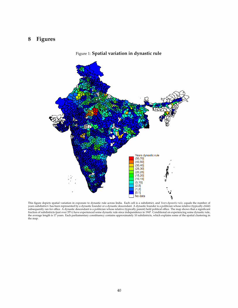
8 Figures

Figure 1: Spatial variation in dynastic rule

This figure depicts spatial variation in exposure to dynastic rule across India. Each cell is a subdistrict, and Years dynastic rulei equals the number ofyears subdistrict i has been represented by a dynastic founder or a dynastic descendant. A dynastic founder is a politician whose relative (typically child)subsequently ran for office. A dynastic descendant is a politician whose relative (typically parent) held political office. The map shows that a significantfraction of subdistricts (just over 35%) have experienced some dynastic rule since independence in 1947. Conditional on experiencing some dynastic rule,the average length is 17 years. Each parliamentary constituency contains approximately 10 subdistricts, which explains some of the spatial clustering inthe map.

40

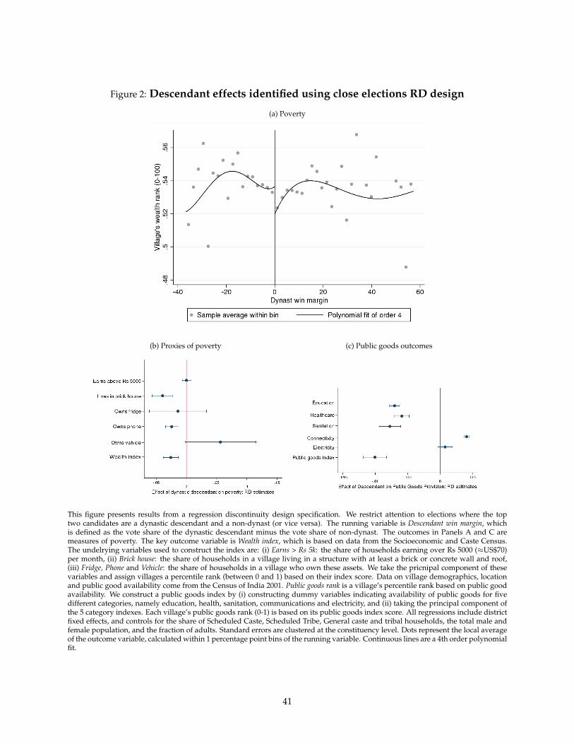
Figure 2: Descendant effects identified using close elections RD design

(a) Poverty

(b) Proxies of poverty (c) Public goods outcomes

This figure presents results from a regression discontinuity design specification. We restrict attention to elections where the toptwo candidates are a dynastic descendant and a non-dynast (or vice versa). The running variable is Descendant win margin, whichis defined as the vote share of the dynastic descendant minus the vote share of non-dynast. The outcomes in Panels A and C aremeasures of poverty. The key outcome variable is Wealth index, which is based on data from the Socioeconomic and Caste Census.The undelrying variables used to construct the index are: (i) Earns > Rs 5k: the share of households earning over Rs 5000 (≈US$70)per month, (ii) Brick house: the share of households in a village living in a structure with at least a brick or concrete wall and roof,(iii) Fridge, Phone and Vehicle: the share of households in a village who own these assets. We take the pricnipal component of thesevariables and assign villages a percentile rank (between 0 and 1) based on their index score. Data on village demographics, locationand public good availability come from the Census of India 2001. Public goods rank is a village’s percentile rank based on public goodavailability. We construct a public goods index by (i) constructing dummy variables indicating availability of public goods for fivedifferent categories, namely education, health, sanitation, communications and electricity, and (ii) taking the principal component ofthe 5 category indexes. Each village’s public goods rank (0-1) is based on its public goods index score. All regressions include districtfixed effects, and controls for the share of Scheduled Caste, Scheduled Tribe, General caste and tribal households, the total male andfemale population, and the fraction of adults. Standard errors are clustered at the constituency level. Dots represent the local averageof the outcome variable, calculated within 1 percentage point bins of the running variable. Continuous lines are a 4th order polynomialfit.

41

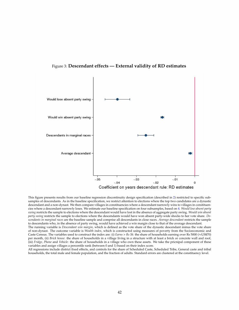
Figure 3: Descendant effects — External validity of RD estimates

This figure presents results from our baseline regression discontinuity design specification (described in 2) restricted to specific sub-samples of descendants. As in the baseline specification, we restrict attention to elections where the top two candidates are a dynasticdescendant and a non-dynast. We then compare villages in constituencies where a descendant narrowly wins to villages in constituen-cies where a descendant narrowly loses. We estimate our baseline specification on four subsamples, based on 4. Would lose absent partyswing restricts the sample to elections where the descendant would have lost in the absence of aggregate party swing. Would win absentparty swing restricts the sample to elections where the descendants would have won absent party-wide shocks to her vote share. De-scendants in marginal races are the baseline sample and comprise all descendants in close races. Average descendant restricts the sampleto descendants who, in the absence of party swing, would have achieved a win margin close to that of the average descendant.The running variable is Descendant win margin, which is defined as the vote share of the dynastic descendant minus the vote shareof non-dynast. The outcome variable is Wealth index, which is constructed using measures of poverty from the Socioeconomic andCaste Census. The variables used to construct the index are: (i) Earns > Rs 5k: the share of households earning over Rs 5000 (≈US$70)per month, (ii) Brick house: the share of households in a village living in a structure with at least a brick or concrete wall and roof,(iii) Fridge, Phone and Vehicle: the share of households in a village who own these assets. We take the pricnipal component of thesevariables and assign villages a percentile rank (between 0 and 1) based on their index score.All regressions include district fixed effects, and controls for the share of Scheduled Caste, Scheduled Tribe, General caste and tribalhouseholds, the total male and female population, and the fraction of adults. Standard errors are clustered at the constituency level.

42

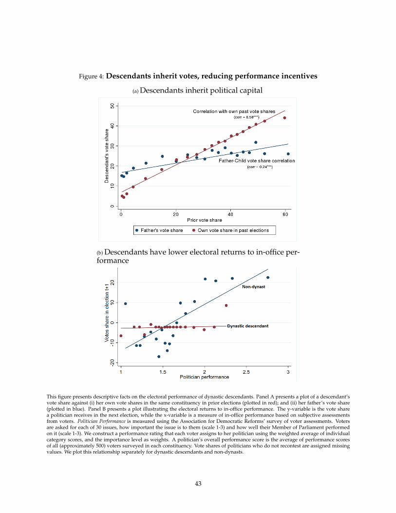
Figure 4: Descendants inherit votes, reducing performance incentives

(a) Descendants inherit political capital

(b) Descendants have lower electoral returns to in-office per-formance

This figure presents descriptive facts on the electoral performance of dynastic descendants. Panel A presents a plot of a descendant’svote share against (i) her own vote shares in the same constituency in prior elections (plotted in red); and (ii) her father’s vote share(plotted in blue). Panel B presents a plot illustrating the electoral returns to in-office performance. The y-variable is the vote sharea politician receives in the next election, while the x-variable is a measure of in-office performance based on subjective assessmentsfrom voters. Politician Performance is measured using the Association for Democratic Reforms’ survey of voter assessments. Votersare asked for each of 30 issues, how important the issue is to them (scale 1-3) and how well their Member of Parliament performedon it (scale 1-3). We construct a performance rating that each voter assigns to her politician using the weighted average of individualcategory scores, and the importance level as weights. A politician’s overall performance score is the average of performance scoresof all (approximately 500) voters surveyed in each constituency. Vote shares of politicians who do not recontest are assigned missingvalues. We plot this relationship separately for dynastic descendants and non-dynasts.

43

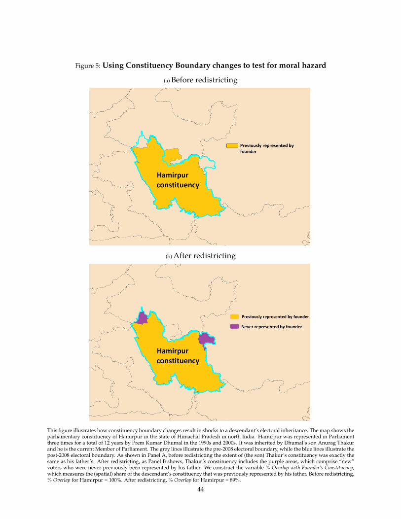
Figure 5: Using Constituency Boundary changes to test for moral hazard

(a) Before redistricting

(b) After redistricting

This figure illustrates how constituency boundary changes result in shocks to a descendant’s electoral inheritance. The map shows theparliamentary constituency of Hamirpur in the state of Himachal Pradesh in north India. Hamirpur was represented in Parliamentthree times for a total of 12 years by Prem Kumar Dhumal in the 1990s and 2000s. It was inherited by Dhumal’s son Anurag Thakurand he is the current Member of Parliament. The grey lines illustrate the pre-2008 electoral boundary, while the blue lines illustrate thepost-2008 electoral boundary. As shown in Panel A, before redistricting the extent of (the son) Thakur’s constituency was exactly thesame as his father’s. After redistricting, as Panel B shows, Thakur’s constituency includes the purple areas, which comprise “new”voters who were never previously been represented by his father. We construct the variable % Overlap with Founder’s Constituency,which measures the (spatial) share of the descendant’s constituency that was previously represented by his father. Before redistricting,% Overlap for Hamirpur = 100%. After redistricting, % Overlap for Hamirpur = 89%.

44

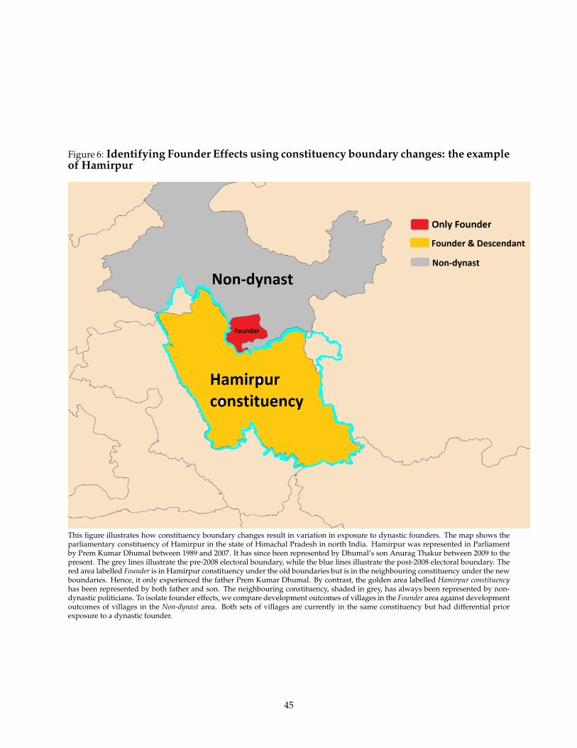
Figure 6: Identifying Founder Effects using constituency boundary changes: the exampleof Hamirpur

This figure illustrates how constituency boundary changes result in variation in exposure to dynastic founders. The map shows theparliamentary constituency of Hamirpur in the state of Himachal Pradesh in north India. Hamirpur was represented in Parliamentby Prem Kumar Dhumal between 1989 and 2007. It has since been represented by Dhumal’s son Anurag Thakur between 2009 to thepresent. The grey lines illustrate the pre-2008 electoral boundary, while the blue lines illustrate the post-2008 electoral boundary. Thered area labelled Founder is in Hamirpur constituency under the old boundaries but is in the neighbouring constituency under the newboundaries. Hence, it only experienced the father Prem Kumar Dhumal. By contrast, the golden area labelled Hamirpur constituencyhas been represented by both father and son. The neighbouring constituency, shaded in grey, has always been represented by non-dynastic politicians. To isolate founder effects, we compare development outcomes of villages in the Founder area against developmentoutcomes of villages in the Non-dynast area. Both sets of villages are currently in the same constituency but had differential priorexposure to a dynastic founder.

45

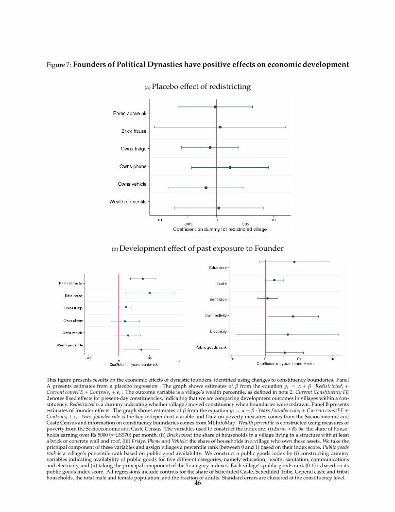
Figure 7: Founders of Political Dynasties have positive effects on economic development

(a) Placebo effect of redistricting

(b) Development effect of past exposure to Founder

This figure presents results on the economic effects of dynastic founders, identified using changes to constituency boundaries. PanelA presents estimates from a placebo regression. The graph shows estimates of β from the equation yi = α + β · Redistrictedi +Current constFE + Controlsi + εi . The outcome variable is a village’s wealth percentile, as defined in note 2. Current Constituency FEdenotes fixed effects for present-day constituencies, indicating that we are comparing development outcomes in villages within a con-stituency. Redistricted is a dummy indicating whether village i moved constituency when boundaries were redrawn. Panel B presentsestimates of founder effects. The graph shows estimates of β from the equation yi = α + β · Years f ounder rulei + Current constFE +Controlsi + εi . Years founder rule is the key independent variable and Data on poverty measures comes from the Socioeconomic andCaste Census and information on constituency boundaries comes from MLInfoMap. Wealth percentile is constructed using measures ofpoverty from the Socioeconomic and Caste Census. The variables used to construct the index are: (i) Earns > Rs 5k: the share of house-holds earning over Rs 5000 (≈US$70) per month, (ii) Brick house: the share of households in a village living in a structure with at leasta brick or concrete wall and roof, (iii) Fridge, Phone and Vehicle: the share of households in a village who own these assets. We take thepricnipal component of these variables and assign villages a percentile rank (between 0 and 1) based on their index score. Public goodsrank is a village’s percentile rank based on public good availability. We construct a public goods index by (i) constructing dummyvariables indicating availability of public goods for five different categories, namely education, health, sanitation, communicationsand electricity, and (ii) taking the principal component of the 5 category indexes. Each village’s public goods rank (0-1) is based on itspublic goods index score. All regressions include controls for the share of Scheduled Caste, Scheduled Tribe, General caste and tribalhouseholds, the total male and female population, and the fraction of adults. Standard errors are clustered at the constituency level.

46

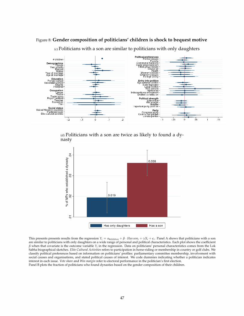
Figure 8: Gender composition of politicians’ children is shock to bequest motive

(c) Politicians with a son are similar to politicians with only daughters

(d) Politicians with a son are twice as likely to found a dy-nasty

This presents presents results from the regression Yi = α#children + β · Has soni + γXi + εi . Panel A shows that politicians with a sonare similar to politicians with only daughters on a wide range of personal and political characteristics. Each plot shows the coefficientβ when that covariate is the outcome variable Yi in the regression. Data on politicians’ personal characteristics comes from the LokSabha biographical sketches. Elite Cultural Activities refers to participation in horse-riding or membership in country or golf clubs. Weclassify political preferences based on information on politicians’ profiles: parliamentary committee membership, involvement withsocial causes and organisations, and stated political causes of interest. We code dummies indicating whether a politician indicatesinterest in each issue. Vote share and Win margin refer to electoral performance in the politician’s first election.Panel B plots the fraction of politicians who found dynasties based on the gender composition of their children.

47

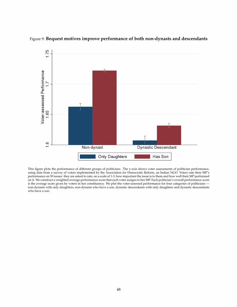
Figure 9: Bequest motives improve performance of both non-dynasts and descendants

This figure plots the performance of different groups of politicians. The y-axis shows voter assessments of politician performance,using data from a survey of voters implemented by the Association for Democratic Reform, an Indian NGO. Voters rate their MP’sperformance on 30 issues: they are asked to rate, on a scale of 1-3, how important the issue is to them and how well their MP performedon it. We construct a weighted average performance score that each voter assigns to her MP. Each politician’s overall performance scoreis the average score given by voters in her constituency. We plot the voter-assessed performance for four categories of politicians —non-dynasts with only daughters, non-dynasts who have a son, dynastic descendants with only daughters and dynastic descendantswho have a son.

48

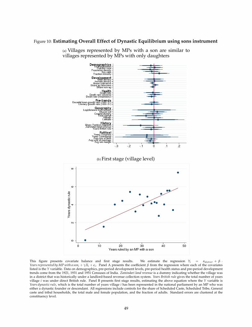
Figure 10: Estimating Overall Effect of Dynastic Equilibrium using sons instrument

(a) Villages represented by MPs with a son are similar tovillages represented by MPs with only daughters

(b) First stage (village level)

This figure presents covariate balance and first stage results. We estimate the regression Yi = αdistrict + β ·Years represented by MP with a soni + γXi + εi . Panel A presents the coefficient β from the regression where each of the covariateslisted is the Y variable. Data on demographics, pre-period development levels, pre-period health status and pre-period developmenttrends come from the 1921, 1931 and 1951 Censuses of India. Zamindari land revenue is a dummy indicating whether the village wasin a district that was historically under a landlord-based revenue collection system. Years British rule gives the total number of yearsvillage i was under direct British rule. Panel B presents first stage results, estimating the above equation where the Y variable isYears dynastic rule, which is the total number of years village i has been represented in the national parliament by an MP who waseither a dynastic founder or descendant. All regressions include controls for the share of Scheduled Caste, Scheduled Tribe, Generalcaste and tribal households, the total male and female population, and the fraction of adults. Standard errors are clustered at theconstituency level.

49

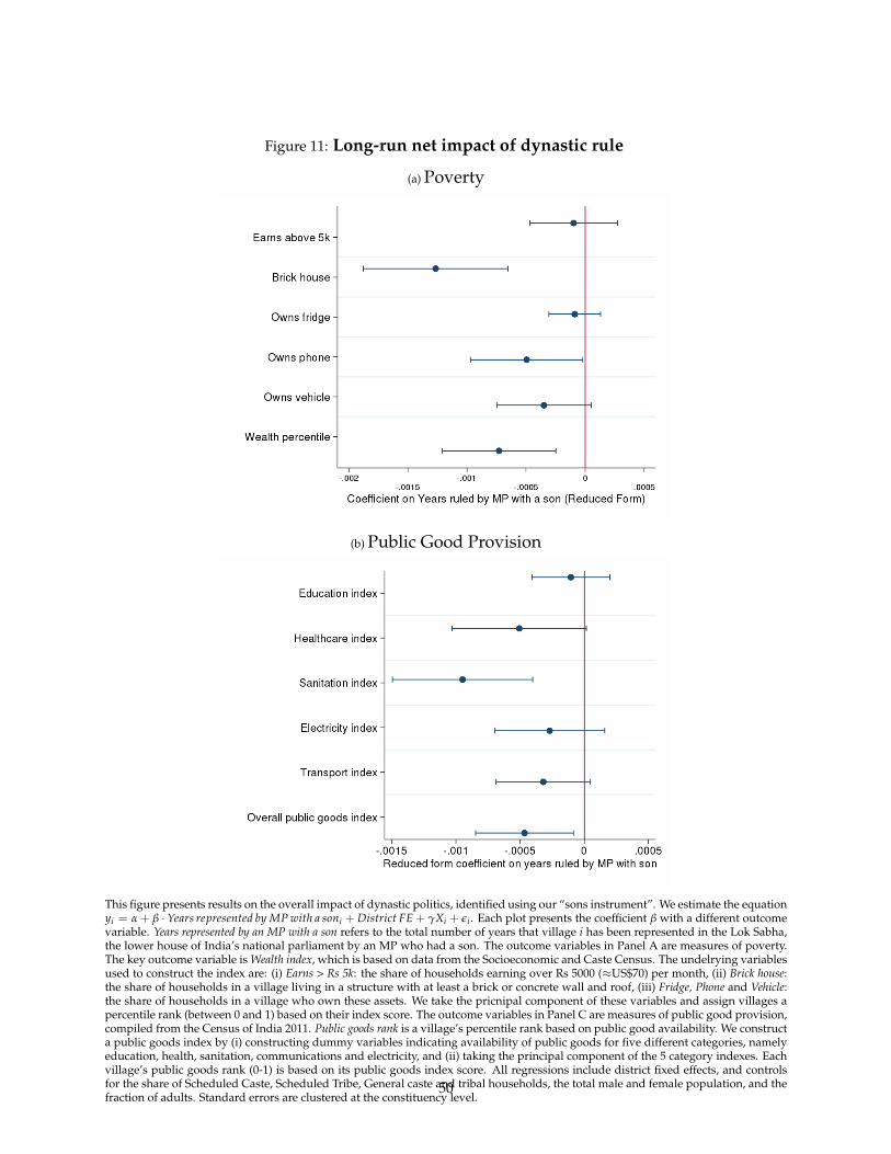
Figure 11: Long-run net impact of dynastic rule

(a) Poverty

(b) Public Good Provision

This figure presents results on the overall impact of dynastic politics, identified using our “sons instrument”. We estimate the equationyi = α + β · Years represented by MP with a soni + District FE + γXi + εi . Each plot presents the coefficient β with a different outcomevariable. Years represented by an MP with a son refers to the total number of years that village i has been represented in the Lok Sabha,the lower house of India’s national parliament by an MP who had a son. The outcome variables in Panel A are measures of poverty.The key outcome variable is Wealth index, which is based on data from the Socioeconomic and Caste Census. The undelrying variablesused to construct the index are: (i) Earns > Rs 5k: the share of households earning over Rs 5000 (≈US$70) per month, (ii) Brick house:the share of households in a village living in a structure with at least a brick or concrete wall and roof, (iii) Fridge, Phone and Vehicle:the share of households in a village who own these assets. We take the pricnipal component of these variables and assign villages apercentile rank (between 0 and 1) based on their index score. The outcome variables in Panel C are measures of public good provision,compiled from the Census of India 2011. Public goods rank is a village’s percentile rank based on public good availability. We constructa public goods index by (i) constructing dummy variables indicating availability of public goods for five different categories, namelyeducation, health, sanitation, communications and electricity, and (ii) taking the principal component of the 5 category indexes. Eachvillage’s public goods rank (0-1) is based on its public goods index score. All regressions include district fixed effects, and controlsfor the share of Scheduled Caste, Scheduled Tribe, General caste and tribal households, the total male and female population, and thefraction of adults. Standard errors are clustered at the constituency level.

50

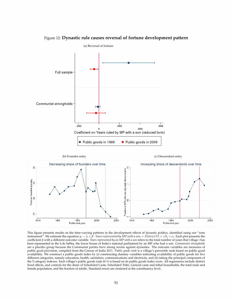
Figure 12: Dynastic rule causes reversal of fortune development pattern

(a) Reversal of fortune

(b) Founder entry (c) Descendant entry

This figure presents results on the time-varying patterns in the development effects of dynastic politics, identified using our “sonsinstrument”. We estimate the equation yi = α + β ·Years represented by MP with a soni + District FE + γXi + εi . Each plot presents thecoefficient β with a different outcome variable. Years represented by an MP with a son refers to the total number of years that village i hasbeen represented in the Lok Sabha, the lower house of India’s national parliament by an MP who had a son. Communist strongholdsare a placebo group because the Communist parties have strong norms against dynasties. The outcome variables are measures ofpublic good provision, compiled from the Census of India 2011. Public goods rank is a village’s percentile rank based on public goodavailability. We construct a public goods index by (i) constructing dummy variables indicating availability of public goods for fivedifferent categories, namely education, health, sanitation, communications and electricity, and (ii) taking the principal component ofthe 5 category indexes. Each village’s public goods rank (0-1) is based on its public goods index score. All regressions include districtfixed effects, and controls for the share of Scheduled Caste, Scheduled Tribe, General caste and tribal households, the total male andfemale population, and the fraction of adults. Standard errors are clustered at the constituency level.

51

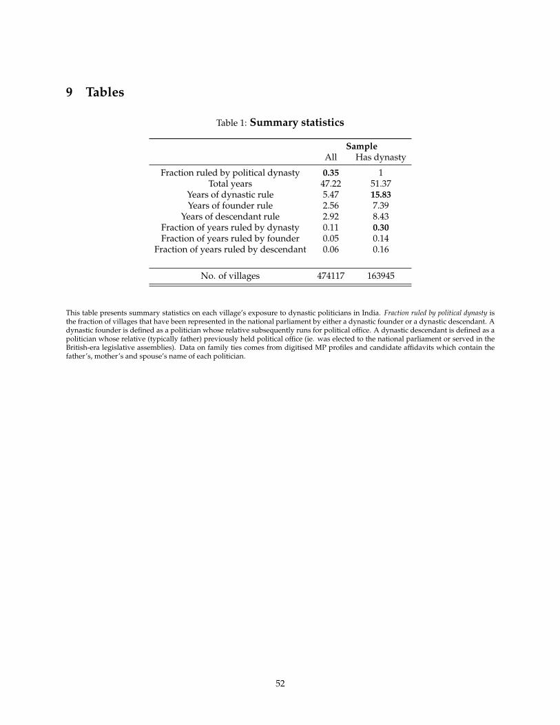
9 Tables

Table 1: Summary statistics

SampleAll Has dynasty

Fraction ruled by political dynasty 0.35 1Total years 47.22 51.37

Years of dynastic rule 5.47 15.83Years of founder rule 2.56 7.39

Years of descendant rule 2.92 8.43Fraction of years ruled by dynasty 0.11 0.30Fraction of years ruled by founder 0.05 0.14

Fraction of years ruled by descendant 0.06 0.16

No. of villages 474117 163945

This table presents summary statistics on each village’s exposure to dynastic politicians in India. Fraction ruled by political dynasty isthe fraction of villages that have been represented in the national parliament by either a dynastic founder or a dynastic descendant. Adynastic founder is defined as a politician whose relative subsequently runs for political office. A dynastic descendant is defined as apolitician whose relative (typically father) previously held political office (ie. was elected to the national parliament or served in theBritish-era legislative assemblies). Data on family ties comes from digitised MP profiles and candidate affidavits which contain thefather’s, mother’s and spouse’s name of each politician.

52

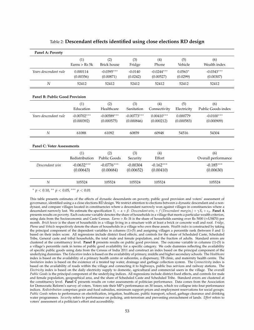
Table 2: Descendant effects identified using close elections RD design

Panel A: Poverty

(1) (2) (3) (4) (5) (6)Earns > Rs 5k Brick house Fridge Phone Vehicle Wealth index

Years descendant rule 0.000114 -0.0395∗∗∗ -0.0140 -0.0244∗∗∗ 0.0563∗ -0.0343∗∗∗

(0.00356) (0.00871) (0.0242) (0.00527) (0.0299) (0.00307)

N 52412 52412 52412 52412 52412 52412

Panel B: Public Good Provision

(1) (2) (3) (4) (5) (6)Education Healthcare Sanitation Connectivity Electricity Public Goods index

Years descendant rule -0.00702∗∗∗ -0.00589∗∗∗ -0.00773∗∗∗ 0.00410∗∗∗ 0.000779 -0.0100∗∗∗

(0.000392) (0.000575) (0.000846) (0.000212) (0.000583) (0.000909)

N 61088 61092 60859 60948 54516 54304

Panel C: Voter Assessments

(1) (2) (3) (4) (6)Redistribution Public Goods Security Effort Overall performance

Descendant win -0.0632∗∗∗ -0.0776∗∗∗ -0.00304 -0.162∗∗∗ -0.185∗∗∗

(0.00643) (0.00684) (0.00652) (0.00410) (0.00630)

N 105524 105524 105524 105524 105524

∗ p < 0.10, ∗∗ p < 0.05, ∗∗∗ p < 0.01

This table presents estimates of the effects of dynastic descendants on poverty, public good provision and voters’ assessment ofgovernance, identified using a a close elections RD design. We restrict attention to elections between a dynastic descendant and a non-dynast, and compare villages located in constituencies where a descendant narrowly won against villages in constituencies where adescendant narrowly lost. We estimate the specification Yi = α + β · Descendant wini + f (Descendant margini) + γXi + εit. Panel Apresents results on poverty. Each outcome variable denotes the share of households in a village that meets a particular wealth criterion,using data from the Socioeconomic and Caste Census. Earns > Rs 5k is the share of households earning over Rs 5000 (≈US$70) permonth. Brick house is the share of households in a village living in a structure with at least a brick or concrete wall and roof. Fridge,Phone and Vehicle respectively denote the share of households in a village who own these assets. Wealth index is constructed by takingthe principal component of the dependent variables in columns (1)-(5) and assigning villages a percentile rank (between 0 and 1)based on their index score. All regressions include district fixed effects, and controls for the share of Scheduled Caste, ScheduledTribe, General caste and tribal households, the total male and female population, and the fraction of adults. Standard errors areclustered at the constituency level. Panel B presents results on public good provision. The outcome variable in columns (1)-(5) isa village’s percentile rank in terms of public good availability for a specific category. We code dummies reflecting the availabilityof specific public goods using data from the Census of India 2011 and construct an index based on the principal component of theunderlying dummies. The Education index is based on the availability of primary, middle and higher secondary schools. The Healthcareindex is based on the availability of a primary health centre or subcentre, a dispensary, TB clinic, and maternity health centre. TheSanitation index is based on the existence of a treated tap water, drainage and garbage collection system. The Connectivity index isbased on the availability of roads within the village and connecting it to highways, public bus services and railway stations. TheElectricity index is based on the daily electricity supply to domestic, agricultural and commercial users in the village. The overallPublic Goods is the principal component of the underlying indices. All regressions include district fixed effects, and controls for maleand female population, geographical area, and the share of Scheduled Caste and Scheduled Tribe. Standard errors are clustered atthe constituency level. Panel C presents results on voter assessments of politician performance. Data comes from the Associationfor Democratic Reform’s survey of voters. Voters rate their MP’s performance on 30 issues, which we collapse into four performanceindices. Redistribution comprises grain and food subsidies, minimum support prices and employment reservations for social groups.Public Goods refers to performance on electrification, irrigation, healthcare, public transport, school, garbage clearance and drinkingwater programmes. Security refers to performance on policing, anti-terrorism and preventing enroachment of lands. Effort refers tovoters’ assessment of a politician’s effort and accessibility.

53

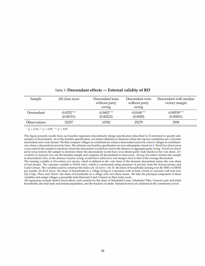
Table 3: Descendant effects — External validity of RD

Sample All close races Descendant loseswithout party

swing

Descendant winswithout party

swing

Descendant with medianvictory margin

Descendant -0.0252∗∗∗ -0.0402∗∗∗ -0.0168∗∗∗ -0.00539∗∗∗

(0.00151) (0.00222) (0.0028) (0.00031)

Observations 32257 10782 25279 3558

∗ p < 0.10, ∗∗ p < 0.05, ∗∗∗ p < 0.01

This figure presents results from our baseline regression discontinuity design specification (described in 2) restricted to specific sub-samples of descendants. As in the baseline specification, we restrict attention to elections where the top two candidates are a dynasticdescendant and a non-dynast. We then compare villages in constituencies where a descendant narrowly wins to villages in constituen-cies where a descendant narrowly loses. We estimate our baseline specification on four subsamples, based on 4. Would lose absent partyswing restricts the sample to elections where the descendant would have lost in the absence of aggregate party swing. Would win absentparty swing restricts the sample to elections where the descendants would have won absent party-wide shocks to her vote share. De-scendants in marginal races are the baseline sample and comprise all descendants in close races. Average descendant restricts the sampleto descendants who, in the absence of party swing, would have achieved a win margin close to that of the average descendant.The running variable is Descendant win margin, which is defined as the vote share of the dynastic descendant minus the vote shareof non-dynast. The outcome variable is Wealth index, which is constructed using measures of poverty from the Socioeconomic andCaste Census. The variables used to construct the index are: (i) Earns > Rs 5k: the share of households earning over Rs 5000 (≈US$70)per month, (ii) Brick house: the share of households in a village living in a structure with at least a brick or concrete wall and roof,(iii) Fridge, Phone and Vehicle: the share of households in a village who own these assets. We take the pricnipal component of thesevariables and assign villages a percentile rank (between 0 and 1) based on their index score.All regressions include district fixed effects, and controls for the share of Scheduled Caste, Scheduled Tribe, General caste and tribalhouseholds, the total male and female population, and the fraction of adults. Standard errors are clustered at the constituency level.

54

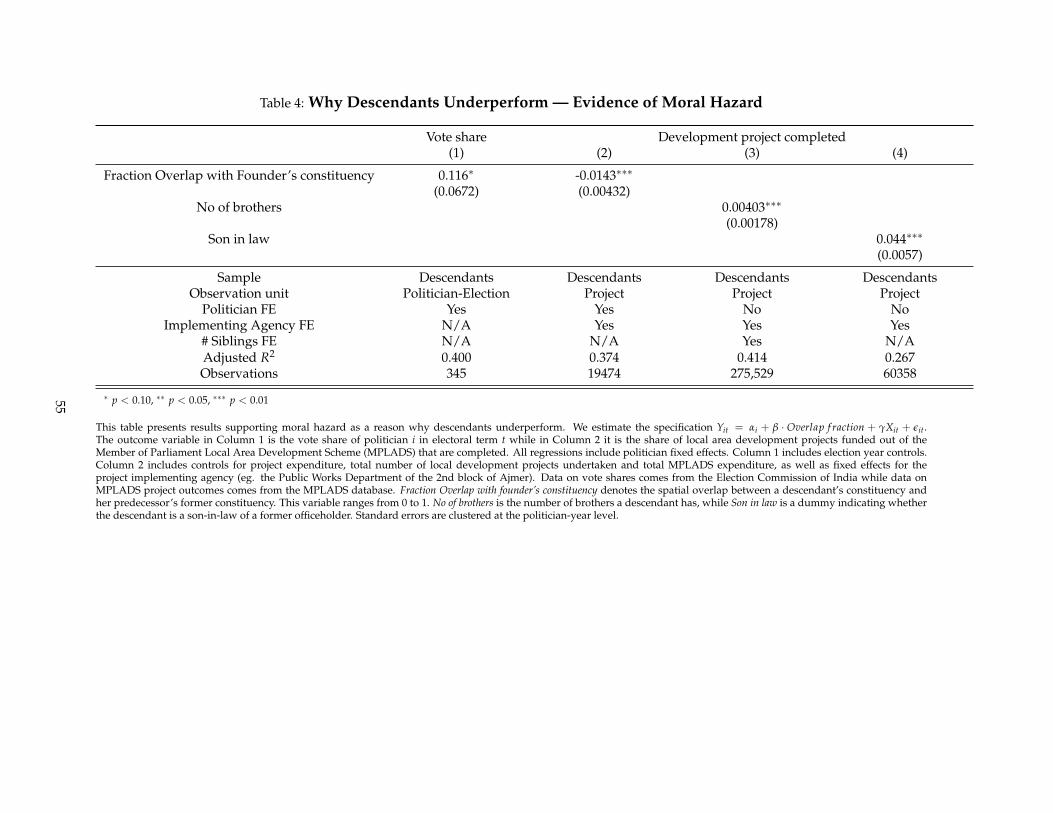
Table 4: Why Descendants Underperform — Evidence of Moral Hazard

Vote share Development project completed(1) (2) (3) (4)

Fraction Overlap with Founder’s constituency 0.116∗ -0.0143∗∗∗

(0.0672) (0.00432)No of brothers 0.00403∗∗∗

(0.00178)Son in law 0.044∗∗∗

(0.0057)

Sample Descendants Descendants Descendants DescendantsObservation unit Politician-Election Project Project Project

Politician FE Yes Yes No NoImplementing Agency FE N/A Yes Yes Yes

# Siblings FE N/A N/A Yes N/AAdjusted R2 0.400 0.374 0.414 0.267Observations 345 19474 275,529 60358

∗ p < 0.10, ∗∗ p < 0.05, ∗∗∗ p < 0.01

This table presents results supporting moral hazard as a reason why descendants underperform. We estimate the specification Yit = αi + β · Overlap f raction + γXit + εit.The outcome variable in Column 1 is the vote share of politician i in electoral term t while in Column 2 it is the share of local area development projects funded out of theMember of Parliament Local Area Development Scheme (MPLADS) that are completed. All regressions include politician fixed effects. Column 1 includes election year controls.Column 2 includes controls for project expenditure, total number of local development projects undertaken and total MPLADS expenditure, as well as fixed effects for theproject implementing agency (eg. the Public Works Department of the 2nd block of Ajmer). Data on vote shares comes from the Election Commission of India while data onMPLADS project outcomes comes from the MPLADS database. Fraction Overlap with founder’s constituency denotes the spatial overlap between a descendant’s constituency andher predecessor’s former constituency. This variable ranges from 0 to 1. No of brothers is the number of brothers a descendant has, while Son in law is a dummy indicating whetherthe descendant is a son-in-law of a former officeholder. Standard errors are clustered at the politician-year level.

55

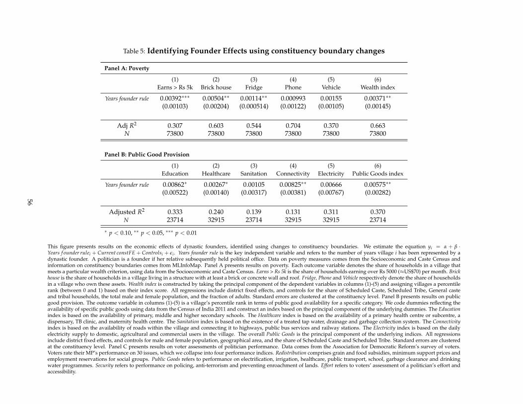
Table 5: Identifying Founder Effects using constituency boundary changes

Panel A: Poverty

(1) (2) (3) (4) (5) (6)Earns > Rs 5k Brick house Fridge Phone Vehicle Wealth index

Years founder rule 0.00392∗∗∗ 0.00504∗∗ 0.00114∗∗ 0.000993 0.00155 0.00371∗∗

(0.00103) (0.00204) (0.000514) (0.00122) (0.00105) (0.00145)

Adj R2 0.307 0.603 0.544 0.704 0.370 0.663N 73800 73800 73800 73800 73800 73800

Panel B: Public Good Provision

(1) (2) (3) (4) (5) (6)Education Healthcare Sanitation Connectivity Electricity Public Goods index

Years founder rule 0.00862∗ 0.00267∗ 0.00105 0.00825∗∗ 0.00666 0.00575∗∗

(0.00522) (0.00140) (0.00317) (0.00381) (0.00767) (0.00282)

Adjusted R2 0.333 0.240 0.139 0.131 0.311 0.370N 23714 32915 23714 32915 32915 23714

∗ p < 0.10, ∗∗ p < 0.05, ∗∗∗ p < 0.01

This figure presents results on the economic effects of dynastic founders, identified using changes to constituency boundaries. We estimate the equation yi = α + β ·Years f ounder rulei + Current constFE + Controlsi + εi . Years founder rule is the key independent variable and refers to the number of years village i has been represented by adynastic founder. A politician is a founder if her relative subsequently held political office. Data on poverty measures comes from the Socioeconomic and Caste Census andinformation on constituency boundaries comes from MLInfoMap. Panel A presents results on poverty. Each outcome variable denotes the share of households in a village thatmeets a particular wealth criterion, using data from the Socioeconomic and Caste Census. Earns > Rs 5k is the share of households earning over Rs 5000 (≈US$70) per month. Brickhouse is the share of households in a village living in a structure with at least a brick or concrete wall and roof. Fridge, Phone and Vehicle respectively denote the share of householdsin a village who own these assets. Wealth index is constructed by taking the principal component of the dependent variables in columns (1)-(5) and assigning villages a percentilerank (between 0 and 1) based on their index score. All regressions include district fixed effects, and controls for the share of Scheduled Caste, Scheduled Tribe, General casteand tribal households, the total male and female population, and the fraction of adults. Standard errors are clustered at the constituency level. Panel B presents results on publicgood provision. The outcome variable in columns (1)-(5) is a village’s percentile rank in terms of public good availability for a specific category. We code dummies reflecting theavailability of specific public goods using data from the Census of India 2011 and construct an index based on the principal component of the underlying dummies. The Educationindex is based on the availability of primary, middle and higher secondary schools. The Healthcare index is based on the availability of a primary health centre or subcentre, adispensary, TB clinic, and maternity health centre. The Sanitation index is based on the existence of a treated tap water, drainage and garbage collection system. The Connectivityindex is based on the availability of roads within the village and connecting it to highways, public bus services and railway stations. The Electricity index is based on the dailyelectricity supply to domestic, agricultural and commercial users in the village. The overall Public Goods is the principal component of the underlying indices. All regressionsinclude district fixed effects, and controls for male and female population, geographical area, and the share of Scheduled Caste and Scheduled Tribe. Standard errors are clusteredat the constituency level. Panel C presents results on voter assessments of politician performance. Data comes from the Association for Democratic Reform’s survey of voters.Voters rate their MP’s performance on 30 issues, which we collapse into four performance indices. Redistribution comprises grain and food subsidies, minimum support prices andemployment reservations for social groups. Public Goods refers to performance on electrification, irrigation, healthcare, public transport, school, garbage clearance and drinkingwater programmes. Security refers to performance on policing, anti-terrorism and preventing enroachment of lands. Effort refers to voters’ assessment of a politician’s effort andaccessibility.

56

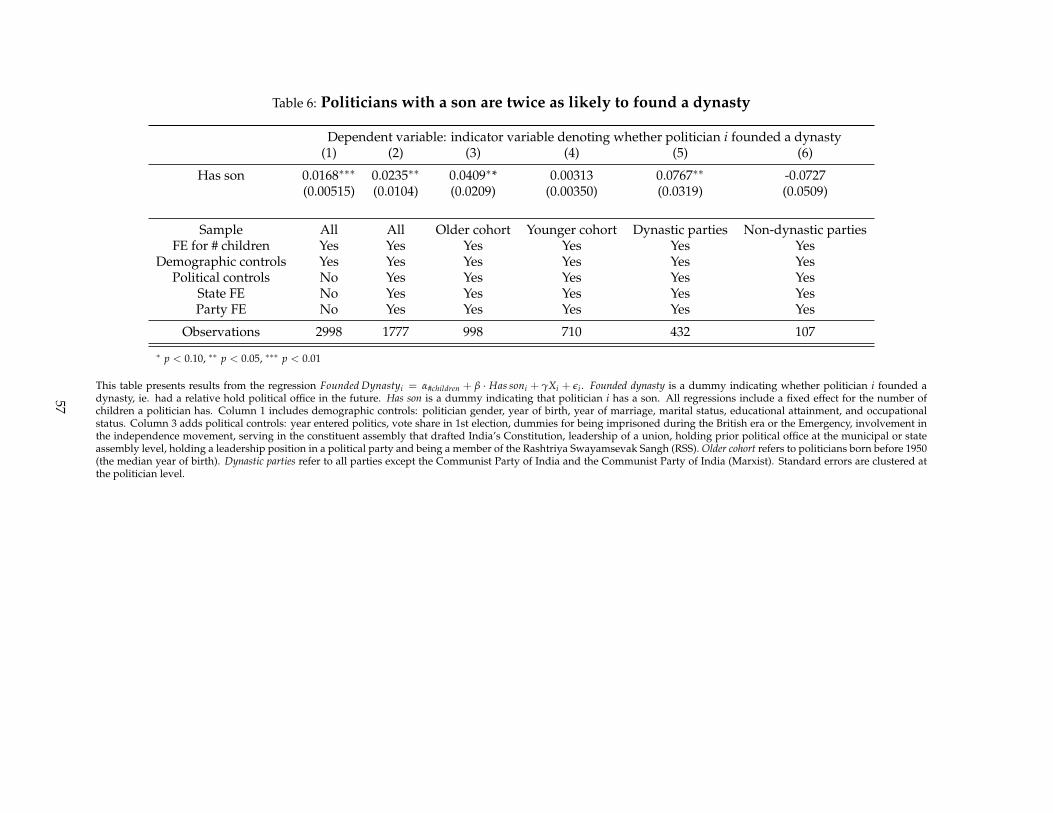
Table 6: Politicians with a son are twice as likely to found a dynasty

Dependent variable: indicator variable denoting whether politician i founded a dynasty(1) (2) (3) (4) (5) (6)

Has son 0.0168∗∗∗ 0.0235∗∗ 0.0409∗* 0.00313 0.0767∗∗ -0.0727(0.00515) (0.0104) (0.0209) (0.00350) (0.0319) (0.0509)

Sample All All Older cohort Younger cohort Dynastic parties Non-dynastic partiesFE for # children Yes Yes Yes Yes Yes Yes

Demographic controls Yes Yes Yes Yes Yes YesPolitical controls No Yes Yes Yes Yes Yes

State FE No Yes Yes Yes Yes YesParty FE No Yes Yes Yes Yes Yes

Observations 2998 1777 998 710 432 107

∗ p < 0.10, ∗∗ p < 0.05, ∗∗∗ p < 0.01

This table presents results from the regression Founded Dynastyi = α#children + β · Has soni + γXi + εi . Founded dynasty is a dummy indicating whether politician i founded adynasty, ie. had a relative hold political office in the future. Has son is a dummy indicating that politician i has a son. All regressions include a fixed effect for the number ofchildren a politician has. Column 1 includes demographic controls: politician gender, year of birth, year of marriage, marital status, educational attainment, and occupationalstatus. Column 3 adds political controls: year entered politics, vote share in 1st election, dummies for being imprisoned during the British era or the Emergency, involvement inthe independence movement, serving in the constituent assembly that drafted India’s Constitution, leadership of a union, holding prior political office at the municipal or stateassembly level, holding a leadership position in a political party and being a member of the Rashtriya Swayamsevak Sangh (RSS). Older cohort refers to politicians born before 1950(the median year of birth). Dynastic parties refer to all parties except the Communist Party of India and the Communist Party of India (Marxist). Standard errors are clustered atthe politician level.

57

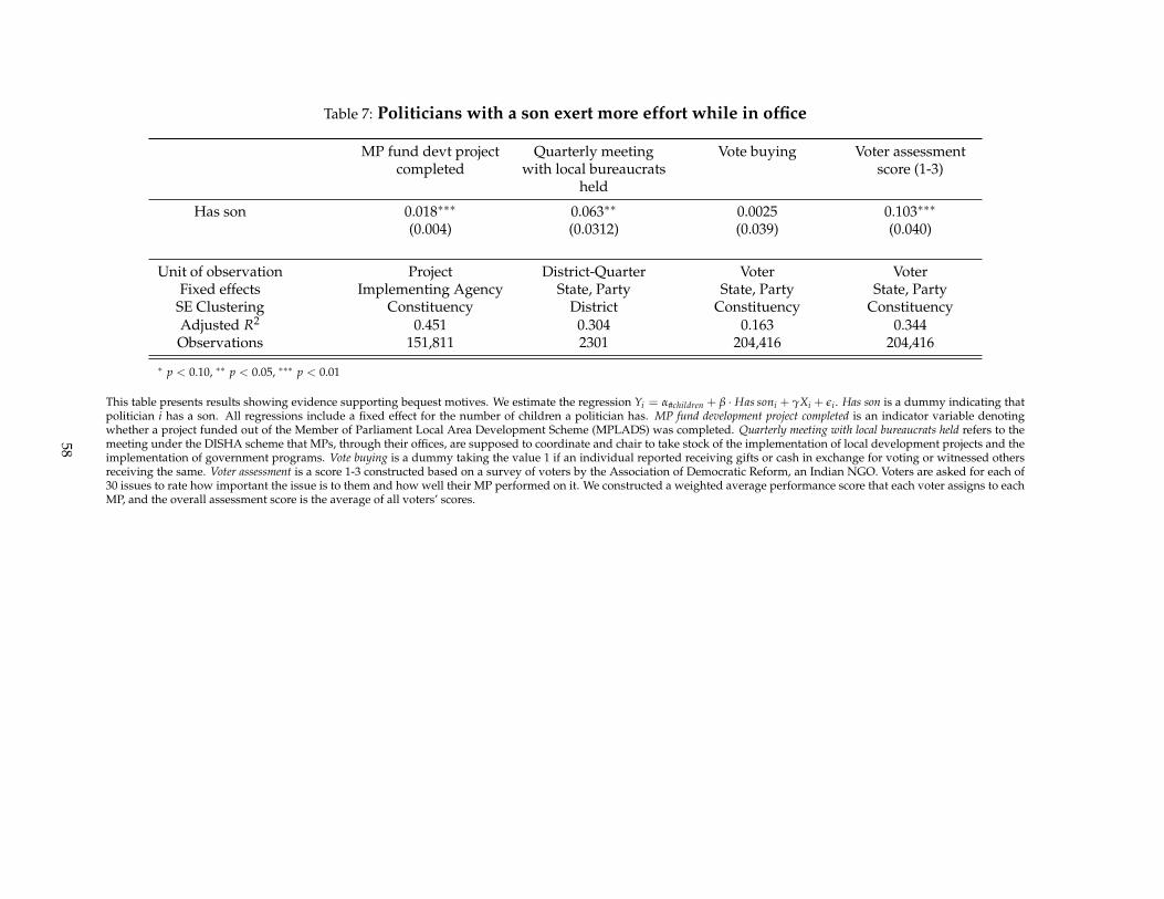
Table 7: Politicians with a son exert more effort while in office

MP fund devt projectcompleted

Quarterly meetingwith local bureaucrats

held

Vote buying Voter assessmentscore (1-3)

Has son 0.018∗∗∗ 0.063∗∗ 0.0025 0.103∗∗∗

(0.004) (0.0312) (0.039) (0.040)

Unit of observation Project District-Quarter Voter VoterFixed effects Implementing Agency State, Party State, Party State, Party

SE Clustering Constituency District Constituency ConstituencyAdjusted R2 0.451 0.304 0.163 0.344Observations 151,811 2301 204,416 204,416

∗ p < 0.10, ∗∗ p < 0.05, ∗∗∗ p < 0.01

This table presents results showing evidence supporting bequest motives. We estimate the regression Yi = α#children + β · Has soni + γXi + εi . Has son is a dummy indicating thatpolitician i has a son. All regressions include a fixed effect for the number of children a politician has. MP fund development project completed is an indicator variable denotingwhether a project funded out of the Member of Parliament Local Area Development Scheme (MPLADS) was completed. Quarterly meeting with local bureaucrats held refers to themeeting under the DISHA scheme that MPs, through their offices, are supposed to coordinate and chair to take stock of the implementation of local development projects and theimplementation of government programs. Vote buying is a dummy taking the value 1 if an individual reported receiving gifts or cash in exchange for voting or witnessed othersreceiving the same. Voter assessment is a score 1-3 constructed based on a survey of voters by the Association of Democratic Reform, an Indian NGO. Voters are asked for each of30 issues to rate how important the issue is to them and how well their MP performed on it. We constructed a weighted average performance score that each voter assigns to eachMP, and the overall assessment score is the average of all voters’ scores.

58

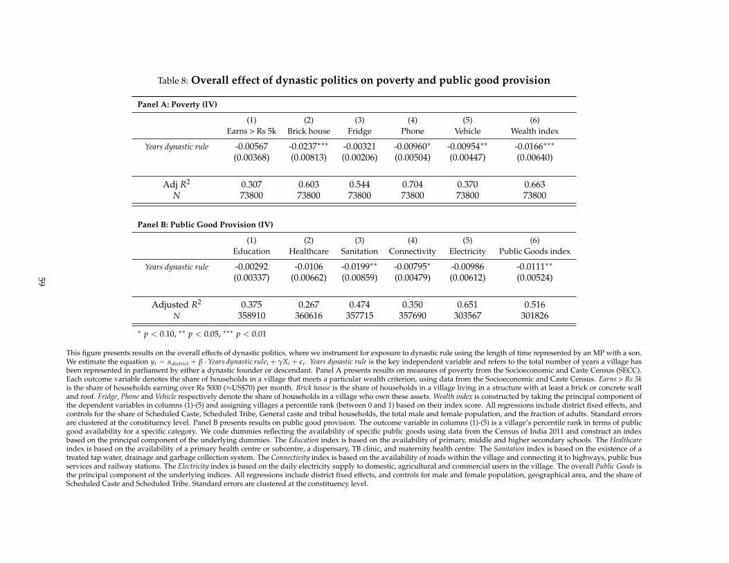
Table 8: Overall effect of dynastic politics on poverty and public good provision

Panel A: Poverty (IV)

(1) (2) (3) (4) (5) (6)Earns > Rs 5k Brick house Fridge Phone Vehicle Wealth index

Years dynastic rule -0.00567 -0.0237∗∗∗ -0.00321 -0.00960∗ -0.00954∗∗ -0.0166∗∗∗

(0.00368) (0.00813) (0.00206) (0.00504) (0.00447) (0.00640)

Adj R2 0.307 0.603 0.544 0.704 0.370 0.663N 73800 73800 73800 73800 73800 73800

Panel B: Public Good Provision (IV)

(1) (2) (3) (4) (5) (6)Education Healthcare Sanitation Connectivity Electricity Public Goods index

Years dynastic rule -0.00292 -0.0106 -0.0199∗∗ -0.00795∗ -0.00986 -0.0111∗∗

(0.00337) (0.00662) (0.00859) (0.00479) (0.00612) (0.00524)

Adjusted R2 0.375 0.267 0.474 0.350 0.651 0.516N 358910 360616 357715 357690 303567 301826

∗ p < 0.10, ∗∗ p < 0.05, ∗∗∗ p < 0.01

This figure presents results on the overall effects of dynastic politics, where we instrument for exposure to dynastic rule using the length of time represented by an MP with a son.We estimate the equation yi = αdistrict + β · Years dynastic rulei + γXi + εi . Years dynastic rule is the key independent variable and refers to the total number of years a village hasbeen represented in parliament by either a dynastic founder or descendant. Panel A presents results on measures of poverty from the Socioeconomic and Caste Census (SECC).Each outcome variable denotes the share of households in a village that meets a particular wealth criterion, using data from the Socioeconomic and Caste Census. Earns > Rs 5kis the share of households earning over Rs 5000 (≈US$70) per month. Brick house is the share of households in a village living in a structure with at least a brick or concrete walland roof. Fridge, Phone and Vehicle respectively denote the share of households in a village who own these assets. Wealth index is constructed by taking the principal component ofthe dependent variables in columns (1)-(5) and assigning villages a percentile rank (between 0 and 1) based on their index score. All regressions include district fixed effects, andcontrols for the share of Scheduled Caste, Scheduled Tribe, General caste and tribal households, the total male and female population, and the fraction of adults. Standard errorsare clustered at the constituency level. Panel B presents results on public good provision. The outcome variable in columns (1)-(5) is a village’s percentile rank in terms of publicgood availability for a specific category. We code dummies reflecting the availability of specific public goods using data from the Census of India 2011 and construct an indexbased on the principal component of the underlying dummies. The Education index is based on the availability of primary, middle and higher secondary schools. The Healthcareindex is based on the availability of a primary health centre or subcentre, a dispensary, TB clinic, and maternity health centre. The Sanitation index is based on the existence of atreated tap water, drainage and garbage collection system. The Connectivity index is based on the availability of roads within the village and connecting it to highways, public busservices and railway stations. The Electricity index is based on the daily electricity supply to domestic, agricultural and commercial users in the village. The overall Public Goods isthe principal component of the underlying indices. All regressions include district fixed effects, and controls for male and female population, geographical area, and the share ofScheduled Caste and Scheduled Tribe. Standard errors are clustered at the constituency level.

59

Appendix

Table of ContentsA Descendant effects: Additional Results 61

A.1 Additional Outcomes . . . . . . . . . . . . . . . . . . . . . . . . . . . . . . . . . . . . . . . . . . 61

A.2 Additional Identification Strategy . . . . . . . . . . . . . . . . . . . . . . . . . . . . . . . . . . . 61

A.3 Additional Mechanisms . . . . . . . . . . . . . . . . . . . . . . . . . . . . . . . . . . . . . . . . 63

B Additional Figures 64

C Additional Tables 77

60

A Descendant effects: Additional Results

A.1 Additional Outcomes

Night time luminosity is increasingly used by development economists and economic geographers as a

proxy for local economic growth. Existing work demonstrates that night light intensity correlates strongly

with human development levels and growth over time (Henderson, Storeygard and Weil 2012; Costinot,

Donaldson and Smith 2016; Donaldson and Storeygard 2016; Bruederle and Hodler 2018). The data come

from images taken by NASA satellites of the world at night. We compile this data at village level for India

from 1992-2013. The advantages of this data are that they are available as an annual panel and at a very fine

spatial level (1km2). We estimate the effects of descendant rule on night time lights growth, using the close

elections RD strategy discussed in 4.1.1.

A.8 presents results from this village-level RD regression. Visually we can see that the results demon-

strate a negative effect of dynastic rule on night lights growth. Next, we include district and subdistrict

fixed effects to control for unobserved district-level factors that affect night time lights growth. Column 1

of table A.7 tells us that dynastic rule reduces village-level night lights growth by 0.44 pp per annum on

average, which is approximately 0.21 std deviations. This effect is sizeable: it is roughly the difference in

growth between a constituency at the 50th percentile of the lights growth distribution (like Mysore) and a

constituency at the 5th percentile (like Dhar in Madhya Pradesh). The effect size and statistical significance

of the coefficient are similar in column 2, where the bandwidth is a dynastic victory margin of 3% rather

than the 5% in column 1. In column 3, we shrink the bandwidth to 1%, and the effect size is much less

precisely estimated. Column 4 shows that including district fixed effects leaves the point estimate virtually

unchanged by increases standard errors, but the coefficient is still statistically significant at the 10% level.

However, introducing subdistrict fixed effects, which is a very restrictive specification, marginally reduces

the point estimate and increases standard errors so that the coefficient is negative but no longer statistically

significant at the 10% level.

A.2 Additional Identification Strategy

In the paper we studied constituency boundary changes for two main purposes. In Section 4.3.2, we used

boundary changes to identify moral hazard as a channel for descendant underperformance. Redistrict-

ing affects the extent of overlap between a descendant’s constituency and his father’s former constituency,

changing the number of votes the same descendant inherits in different elections. Then, in Section 5, we

61

used boundary changes to identify founder effects. Some villages represented by the founder are redis-

tricted into a neighbouring constituency before the descendant enters politics, allowing to identify the ef-

fects of being represented by a founder but not a descendant.

We can also conduct the opposite exercise and use redistricting to identify descendant effects. Some

villages never represented by the founder are redistricted into a descendant’s constituency, and we can in

theory use this variation to identify the effects of exposure to a descendant but not a founder. In other

words, we would look at villages that were previously in the same constituency (represented by a non-

dynast), and compare villages that were redistricted into a descendant’s constituency against those that

remained behind in the original constituency. This identification strategy would be complementary to the

close elections RD design we described in Section 4.1.1. Specifically, we estimate

yi = αold constituency + β ·Years descendant rulei + γXi + εi

where i denotes a village, yi denotes poverty and public good outcomes of village i and αconstituency

is a fixed effect for each pre-boundary change constituency. Figure A.10 presents results on descendant

effects. In contrast to founders, descendants appear to have a negative impact on economic outcomes,

though the effects are statistically weaker. An additional year of exposure to descendants lowers the share

of households who (i) earn above Rs 5k by 0.3pp, (ii) own a fridge by 0.2pp, (iii) own a vehicle by 0.9pp.

However, only the coefficient on vehicle ownership is statistically significant at the 5% level. Moreover, the

point estimates on living in a brick house is actually positive though insignificant. In sum, an extra year of

exposure to descendants lowers a village’s wealth rank by 0.3pp (so a standard deviation would lower the

wealth rank by 2.4pp), though again this effect is not significant. We believe the weaker results from this

identification strategy are due to the following: the identifying variation of this empirical strategy comes

from villages that were redistricted into a descendant’s constituency during the boundary change exercise

of 2008, which took effect after the parliamentary election of 2009. Our outcomes are measured in 2011-12,

giving very little time for stock measures of poverty — such as share of population living in a brick house

— to change.

62

A.3 Additional Mechanisms

A.3.1 Name recognition

Dynasts inherit a bundle of political assets from their predecessors that confer electoral advantage. One

of these things is a prominent name. Political scientists have presented empirical evidence supporting the

claim that name recognition increases a candidate’s vote share (Kam and Zechmeister 2013). In this sec-

tion we compare the electoral advantages of descendants against a group of non-dynastic politicians who

nonetheless have name recognition amongst voters — celebrities. Several film stars and sportspeople (typi-

cally cricketers) have entered politics, and we can thus compare both the electoral and in-office performance

of celebrities and dynastic descendants. Table A.8 shows that celebrities do not seem to have large electoral

advantages and do not appear to perform worse in office, while dynasts on average have an electoral ad-

vantage of 2.4pp and perform worse in office (based on the RD). However, the point estimates on both

electoral advantage and in-office performance are similar for both dynasts and celebrity politicians, and we

are unable to reject that both sets of coefficients are different.

63

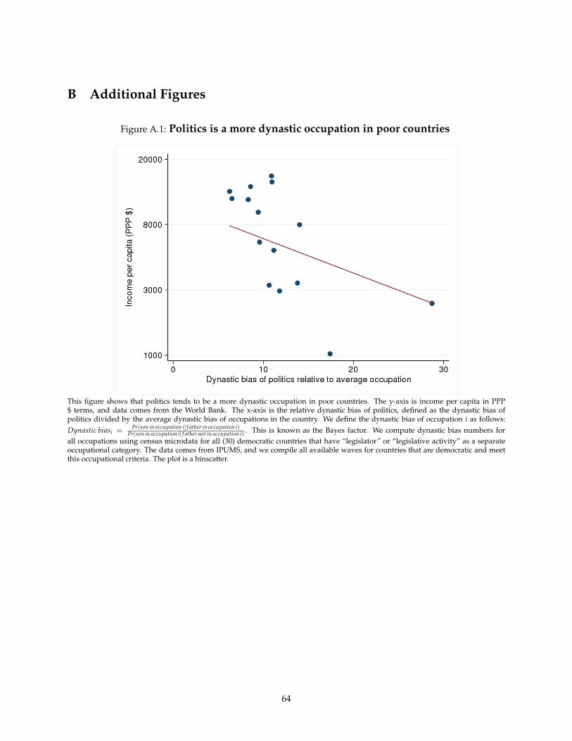
B Additional Figures

Figure A.1: Politics is a more dynastic occupation in poor countries

This figure shows that politics tends to be a more dynastic occupation in poor countries. The y-axis is income per capita in PPP$ terms, and data comes from the World Bank. The x-axis is the relative dynastic bias of politics, defined as the dynastic bias ofpolitics divided by the average dynastic bias of occupations in the country. We define the dynastic bias of occupation i as follows:Dynastic biasi = Pr(son in occupation i| f ather in occupation i)

Pr(son in occupation i| f ather not in occupation i) . This is known as the Bayes factor. We compute dynastic bias numbers forall occupations using census microdata for all (30) democratic countries that have “legislator” or “legislative activity” as a separateoccupational category. The data comes from IPUMS, and we compile all available waves for countries that are democratic and meetthis occupational criteria. The plot is a binscatter.

64

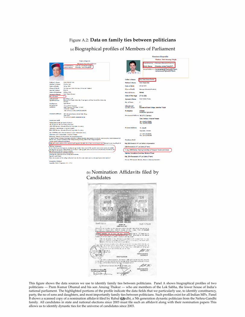
Figure A.2: Data on family ties between politicians

(a) Biographical profiles of Members of Parliament

(b) Nomination Affidavits filed byCandidates

This figure shows the data sources we use to identify family ties between politicians. Panel A shows biographical profiles of twopoliticians — Prem Kumar Dhumal and his son Anurag Thakur — who are members of the Lok Sabha, the lower house of India’snational parliament. The highlighted portions of the profile indicate the data fields that we particularly use, to identify constituency,party, the no of sons and daughters, and most importantly family ties between politicians. Such profiles exist for all Indian MPs. PanelB shows a scanned copy of a nomination affidavit filed by Rahul Gandhi, a 5th generation dynastic politician from the Nehru-Gandhifamily. All candidates in state and national elections since 2003 must file such an affidavit along with their nomination papers Thisallows us to identify dynastic ties for the universe of candidates since 2003.

65

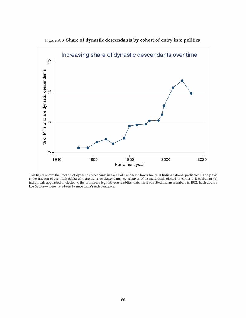
Figure A.3: Share of dynastic descendants by cohort of entry into politics

This figure shows the fraction of dynastic descendants in each Lok Sabha, the lower house of India’s national parliament. The y-axisis the fraction of each Lok Sabha who are dynastic descendants ie. relatives of (i) individuals elected to earlier Lok Sabhas or (ii)individuals appointed or elected to the British-era legislative assemblies which first admitted Indian members in 1862. Each dot is aLok Sabha — there have been 16 since India’s independence.

66

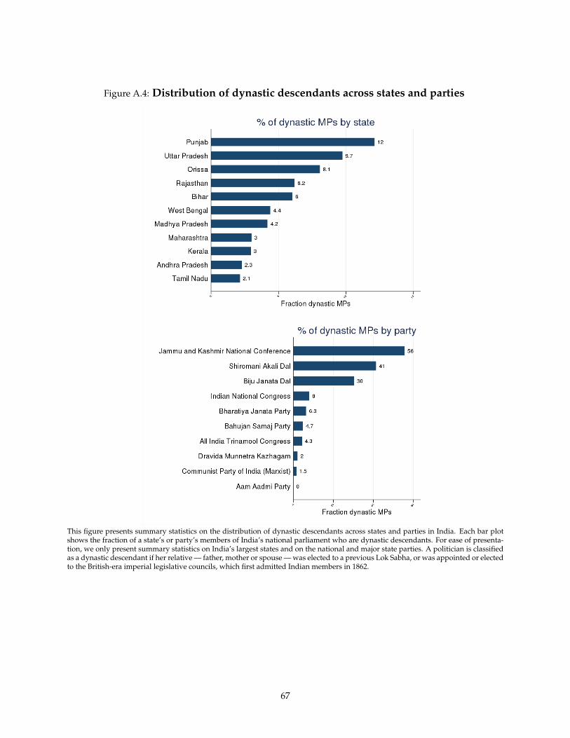
Figure A.4: Distribution of dynastic descendants across states and parties

This figure presents summary statistics on the distribution of dynastic descendants across states and parties in India. Each bar plotshows the fraction of a state’s or party’s members of India’s national parliament who are dynastic descendants. For ease of presenta-tion, we only present summary statistics on India’s largest states and on the national and major state parties. A politician is classifiedas a dynastic descendant if her relative — father, mother or spouse — was elected to a previous Lok Sabha, or was appointed or electedto the British-era imperial legislative councils, which first admitted Indian members in 1862.

67

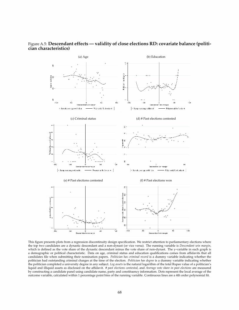
Figure A.5: Descendant effects — validity of close elections RD: covariate balance (politi-cian characteristics)

(a) Age (b) Education

(c) Criminal status (d) # Past elections contested

(e) # Past elections contested (f) # Past elections won

This figure presents plots from a regression discontinuity design specification. We restrict attention to parliamentary elections wherethe top two candidates are a dynastic descendant and a non-dynast (or vice versa). The running variable is Descendant win margin,which is defined as the vote share of the dynastic descendant minus the vote share of non-dynast. The y-variable in each graph isa demographic or political characteristic. Data on age, criminal status and education qualifications comes from affidavits that allcandidates file when submitting their nomination papers. Politician has criminal record is a dummy variable indicating whether thepolitician had outstanding criminal charges at the time of the election. Politician has degree is a dummy variable indicating whetherthe politician completed a university degree in any subject. Log assets is the natural logarithm of the total Rupee value of a politician’sliquid and illiquid assets as disclosed on the affidavit. # past elections contested, and Average vote share in past elections are measuredby constructing a candidate panel using candidate name, party and constituency information. Dots represent the local average of theoutcome variable, calculated within 1 percentage point bins of the running variable. Continuous lines are a 4th order polynomial fit.

68

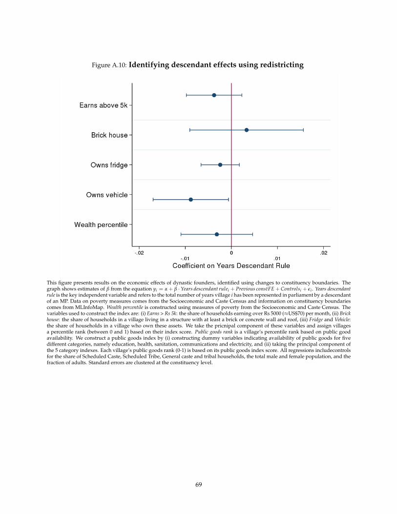
Figure A.10: Identifying descendant effects using redistricting

This figure presents results on the economic effects of dynastic founders, identified using changes to constituency boundaries. Thegraph shows estimates of β from the equation yi = α + β · Years descendant rulei + Previous constFE + Controlsi + εi . Years descendantrule is the key independent variable and refers to the total number of years village i has been represented in parliament by a descendantof an MP. Data on poverty measures comes from the Socioeconomic and Caste Census and information on constituency boundariescomes from MLInfoMap. Wealth percentile is constructed using measures of poverty from the Socioeconomic and Caste Census. Thevariables used to construct the index are: (i) Earns > Rs 5k: the share of households earning over Rs 5000 (≈US$70) per month, (ii) Brickhouse: the share of households in a village living in a structure with at least a brick or concrete wall and roof, (iii) Fridge and Vehicle:the share of households in a village who own these assets. We take the pricnipal component of these variables and assign villagesa percentile rank (between 0 and 1) based on their index score. Public goods rank is a village’s percentile rank based on public goodavailability. We construct a public goods index by (i) constructing dummy variables indicating availability of public goods for fivedifferent categories, namely education, health, sanitation, communications and electricity, and (ii) taking the principal component ofthe 5 category indexes. Each village’s public goods rank (0-1) is based on its public goods index score. All regressions includecontrolsfor the share of Scheduled Caste, Scheduled Tribe, General caste and tribal households, the total male and female population, and thefraction of adults. Standard errors are clustered at the constituency level.

69

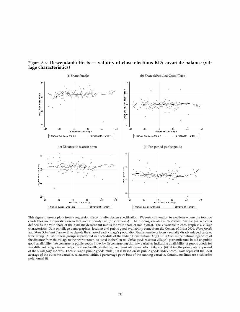
Figure A.6: Descendant effects — validity of close elections RD: covariate balance (vil-lage characteristics)

(a) Share female (b) Share Scheduled Caste/Tribe

(c) Distance to nearest town (d) Pre-period public goods

This figure presents plots from a regression discontinuity design specification. We restrict attention to elections where the top twocandidates are a dynastic descendant and a non-dynast (or vice versa). The running variable is Descendant win margin, which isdefined as the vote share of the dynastic descendant minus the vote share of non-dynast. The y-variable in each graph is a villagecharacteristic. Data on village demographics, location and public good availability come from the Census of India 2001. Share femaleand Share Scheduled Caste or Tribe denote the share of each village’s population that is female or from a socially disadvantaged caste ortribe group. A list of these groups is provided in a schedule of the Indian Constitution. Log Dist to town is the natural logarithm ofthe distance from the village to the nearest town, as listed in the Census. Public goods rank is a village’s percentile rank based on publicgood availability. We construct a public goods index by (i) constructing dummy variables indicating availability of public goods forfive different categories, namely education, health, sanitation, communications and electricity, and (ii) taking the principal componentof the 5 category indexes. Each village’s public goods rank (0-1) is based on its public goods index score. Dots represent the localaverage of the outcome variable, calculated within 1 percentage point bins of the running variable. Continuous lines are a 4th orderpolynomial fit.

70

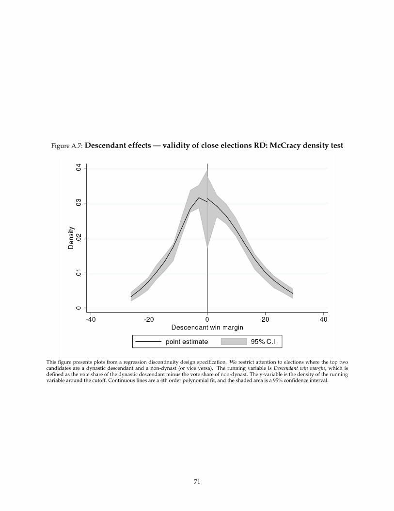
Figure A.7: Descendant effects — validity of close elections RD: McCracy density test

This figure presents plots from a regression discontinuity design specification. We restrict attention to elections where the top twocandidates are a dynastic descendant and a non-dynast (or vice versa). The running variable is Descendant win margin, which isdefined as the vote share of the dynastic descendant minus the vote share of non-dynast. The y-variable is the density of the runningvariable around the cutoff. Continuous lines are a 4th order polynomial fit, and the shaded area is a 95% confidence interval.

71

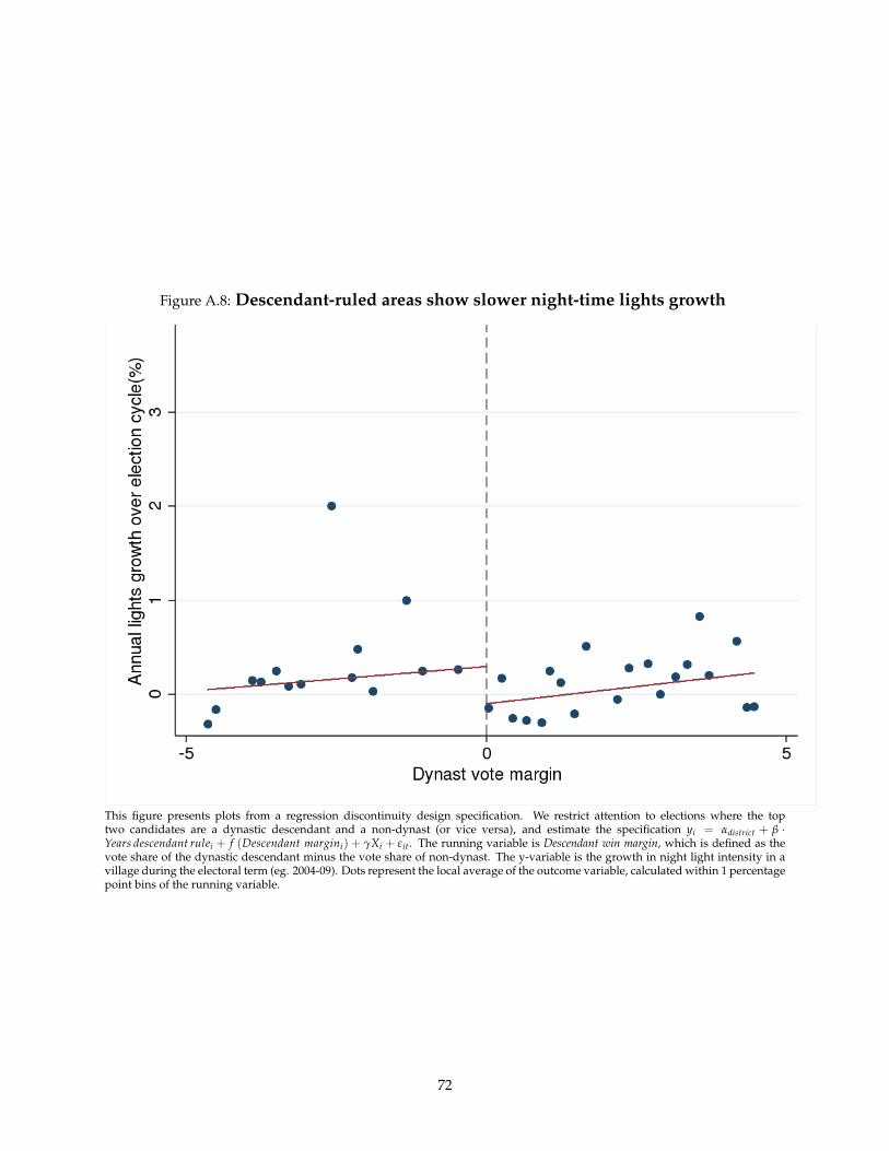
Figure A.8: Descendant-ruled areas show slower night-time lights growth

This figure presents plots from a regression discontinuity design specification. We restrict attention to elections where the toptwo candidates are a dynastic descendant and a non-dynast (or vice versa), and estimate the specification yi = αdistrict + β ·Years descendant rulei + f (Descendant margini) + γXi + εit. The running variable is Descendant win margin, which is defined as thevote share of the dynastic descendant minus the vote share of non-dynast. The y-variable is the growth in night light intensity in avillage during the electoral term (eg. 2004-09). Dots represent the local average of the outcome variable, calculated within 1 percentagepoint bins of the running variable.

72

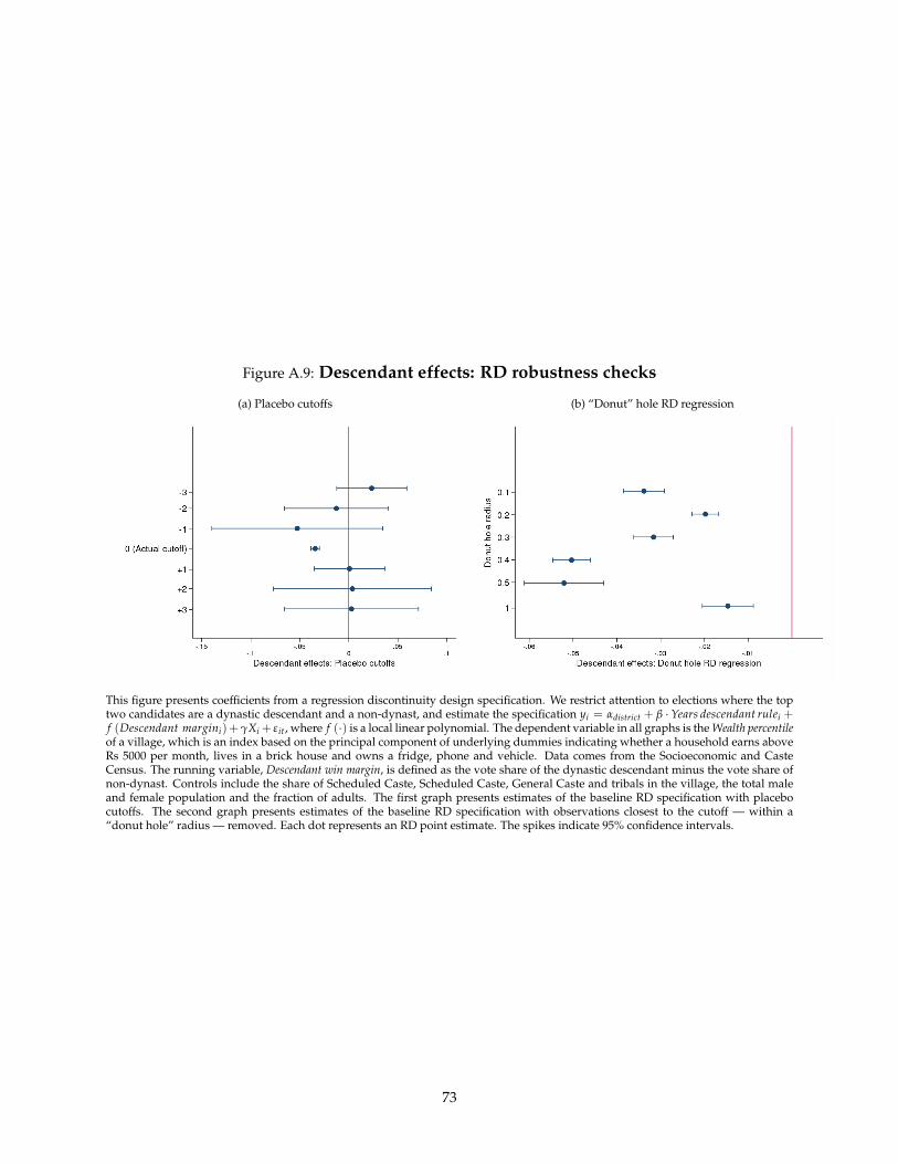
Figure A.9: Descendant effects: RD robustness checks

(a) Placebo cutoffs (b) “Donut” hole RD regression

This figure presents coefficients from a regression discontinuity design specification. We restrict attention to elections where the toptwo candidates are a dynastic descendant and a non-dynast, and estimate the specification yi = αdistrict + β · Years descendant rulei +f (Descendant margini)+γXi + εit, where f (·) is a local linear polynomial. The dependent variable in all graphs is the Wealth percentileof a village, which is an index based on the principal component of underlying dummies indicating whether a household earns aboveRs 5000 per month, lives in a brick house and owns a fridge, phone and vehicle. Data comes from the Socioeconomic and CasteCensus. The running variable, Descendant win margin, is defined as the vote share of the dynastic descendant minus the vote share ofnon-dynast. Controls include the share of Scheduled Caste, Scheduled Caste, General Caste and tribals in the village, the total maleand female population and the fraction of adults. The first graph presents estimates of the baseline RD specification with placebocutoffs. The second graph presents estimates of the baseline RD specification with observations closest to the cutoff — within a“donut hole” radius — removed. Each dot represents an RD point estimate. The spikes indicate 95% confidence intervals.

73

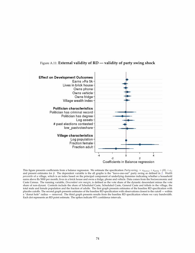
Figure A.11: External validity of RD — validity of party swing shock

This figure presents coefficients from a balance regression. We estimate the specification Party swingi = αdistrict + αparty + βXi + εi ,and present estimates for β. The dependent variable is the all graphs is the “leave-one-out” party swing as defined in 2. Wealthpercentile of a village, which is an index based on the principal component of underlying dummies indicating whether a householdearns above Rs 5000 per month, lives in a brick house and owns a fridge, phone and vehicle. Data comes from the Socioeconomic andCaste Census. The running variable, Descendant win margin, is defined as the vote share of the dynastic descendant minus the voteshare of non-dynast. Controls include the share of Scheduled Caste, Scheduled Caste, General Caste and tribals in the village, thetotal male and female population and the fraction of adults. The first graph presents estimates of the baseline RD specification withplacebo cutoffs. The second graph presents estimates of the baseline RD specification with observations closest to the cutoff — withina “donut hole” radius — removed. The third graph presents results from the baseline RD specification where we vary bandwidth.Each dot represents an RD point estimate. The spikes indicate 95% confidence intervals.

74

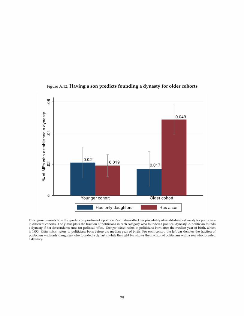
Figure A.12: Having a son predicts founding a dynasty for older cohorts

This figure presents how the gender composition of a politician’s children affect her probability of establishing a dynasty for politiciansin different cohorts. The y-axis plots the fraction of politicians in each category who founded a political dynasty. A politician foundsa dynasty if her descendants runs for political office. Younger cohort refers to politicians born after the median year of birth, whichis 1950. Older cohort refers to politicians born before the median year of birth. For each cohort, the left bar denotes the fraction ofpoliticians with only daughters who founded a dynasty, while the right bar shows the fraction of politicians with a son who foundeda dynasty.

75

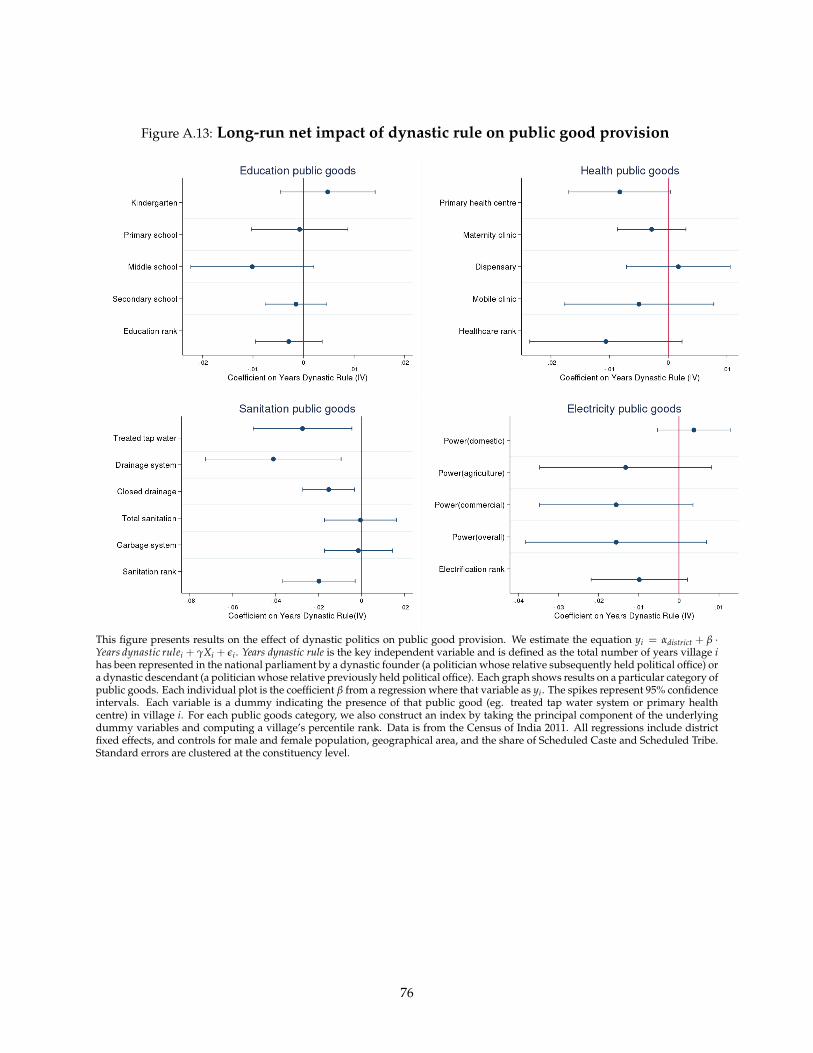
Figure A.13: Long-run net impact of dynastic rule on public good provision

This figure presents results on the effect of dynastic politics on public good provision. We estimate the equation yi = αdistrict + β ·Years dynastic rulei + γXi + εi . Years dynastic rule is the key independent variable and is defined as the total number of years village ihas been represented in the national parliament by a dynastic founder (a politician whose relative subsequently held political office) ora dynastic descendant (a politician whose relative previously held political office). Each graph shows results on a particular category ofpublic goods. Each individual plot is the coefficient β from a regression where that variable as yi . The spikes represent 95% confidenceintervals. Each variable is a dummy indicating the presence of that public good (eg. treated tap water system or primary healthcentre) in village i. For each public goods category, we also construct an index by taking the principal component of the underlyingdummy variables and computing a village’s percentile rank. Data is from the Census of India 2011. All regressions include districtfixed effects, and controls for male and female population, geographical area, and the share of Scheduled Caste and Scheduled Tribe.Standard errors are clustered at the constituency level.

76

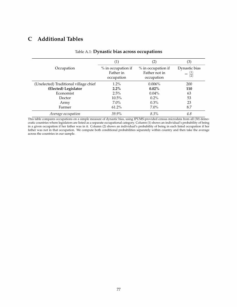
C Additional Tables

Table A.1: Dynastic bias across occupations

(1) (2) (3)

Occupation % in occupation ifFather in

occupation

% in occupation ifFather not inoccupation

Dynastic bias= (1)

(2)

(Unelected) Traditional village chief 1.2% 0.006% 200(Elected) Legislator 2.2% 0.02% 110

Economist 2.5% 0.04% 63Doctor 10.5% 0.2% 53Army 7.0% 0.3% 23

Farmer 61.2% 7.0% 8.7

Average occupation 39.9% 8.3% 4.8This table compares occupations on a simple measure of dynastic bias, using IPUMS-provided census microdata from all (30) demo-cratic countries where legislators are listed as a separate occupational category. Column (1) shows an individual’s probability of beingin a given occupation if her father was in it. Column (2) shows an individual’s probability of being in each listed occupation if herfather was not in that occupation. We compute both conditional probabilities separately within country and then take the averageacross the countries in our sample.

77

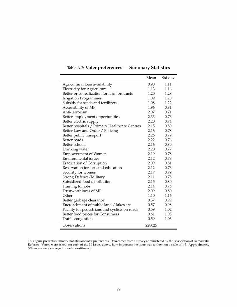
Table A.2: Voter preferences — Summary Statistics

Mean Std dev

Agricultural loan availability 0.98 1.11Electricity for Agriculture 1.13 1.16Better price-realization for farm products 1.20 1.28Irrigation Programmes 1.09 1.20Subsidy for seeds and fertilizers 1.08 1.22Accessibility of MP 1.96 0.81Anti-terrorism 2.07 0.71Better employment opportunities 2.33 0.76Better electric supply 2.20 0.74Better hospitals / Primary Healthcare Centres 2.15 0.80Better Law and Order / Policing 2.16 0.78Better public transport 2.26 0.79Better roads 2.22 0.76Better schools 2.16 0.80Drinking water 2.20 0.77Empowerment of Women 2.19 0.78Environmental issues 2.12 0.78Eradication of Corruption 2.09 0.81Reservation for jobs and education 2.12 0.76Security for women 2.17 0.79Strong Defence/Military 2.11 0.78Subsidized food distribution 2.15 0.80Training for jobs 2.14 0.76Trustworthiness of MP 2.09 0.80Other 1.10 1.16Better garbage clearance 0.57 0.99Encroachment of public land / lakes etc 0.57 0.98Facility for pedestrians and cyclists on roads 0.59 1.02Better food prices for Consumers 0.61 1.05Traffic congestion 0.59 1.03

Observations 228025

This figure presents summary statistics on voter preferences. Data comes from a survey administered by the Association of DemocraticReforms. Voters were asked, for each of the 30 issues above, how important the issue was to them on a scale of 1-3. Approximately500 voters were surveyed in each constituency.

78

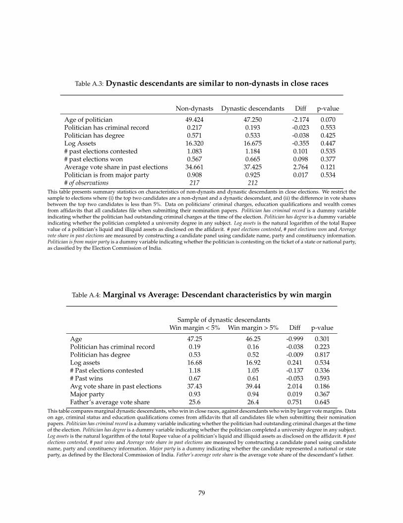
Table A.3: Dynastic descendants are similar to non-dynasts in close races

Non-dynasts Dynastic descendants Diff p-value

Age of politician 49.424 47.250 -2.174 0.070Politician has criminal record 0.217 0.193 -0.023 0.553Politician has degree 0.571 0.533 -0.038 0.425Log Assets 16.320 16.675 -0.355 0.447# past elections contested 1.083 1.184 0.101 0.535# past elections won 0.567 0.665 0.098 0.377Average vote share in past elections 34.661 37.425 2.764 0.121Politician is from major party 0.908 0.925 0.017 0.534# of observations 217 212

This table presents summary statistics on characteristics of non-dynasts and dynastic descendants in close elections. We restrict thesample to elections where (i) the top two candidates are a non-dynast and a dynastic descendant, and (ii) the difference in vote sharesbetween the top two candidates is less than 5%. Data on politicians’ criminal charges, education qualifications and wealth comesfrom affidavits that all candidates file when submitting their nomination papers. Politician has criminal record is a dummy variableindicating whether the politician had outstanding criminal charges at the time of the election. Politician has degree is a dummy variableindicating whether the politician completed a university degree in any subject. Log assets is the natural logarithm of the total Rupeevalue of a politician’s liquid and illiquid assets as disclosed on the affidavit. # past elections contested, # past elections won and Averagevote share in past elections are measured by constructing a candidate panel using candidate name, party and constituency information.Politician is from major party is a dummy variable indicating whether the politician is contesting on the ticket of a state or national party,as classified by the Election Commission of India.

Table A.4: Marginal vs Average: Descendant characteristics by win margin

Sample of dynastic descendantsWin margin < 5% Win margin > 5% Diff p-value

Age 47.25 46.25 -0.999 0.301Politician has criminal record 0.19 0.16 -0.038 0.223Politician has degree 0.53 0.52 -0.009 0.817Log assets 16.68 16.92 0.241 0.534# Past elections contested 1.18 1.05 -0.137 0.336# Past wins 0.67 0.61 -0.053 0.593Avg vote share in past elections 37.43 39.44 2.014 0.186Major party 0.93 0.94 0.019 0.367Father’s average vote share 25.6 26.4 0.751 0.645

This table compares marginal dynastic descendants, who win in close races, against descendants who win by larger vote margins. Dataon age, criminal status and education qualifications comes from affidavits that all candidates file when submitting their nominationpapers. Politician has criminal record is a dummy variable indicating whether the politician had outstanding criminal charges at the timeof the election. Politician has degree is a dummy variable indicating whether the politician completed a university degree in any subject.Log assets is the natural logarithm of the total Rupee value of a politician’s liquid and illiquid assets as disclosed on the affidavit. # pastelections contested, # past wins and Average vote share in past elections are measured by constructing a candidate panel using candidatename, party and constituency information. Major party is a dummy indicating whether the candidate represented a national or stateparty, as defined by the Electoral Commission of India. Father’s average vote share is the average vote share of the descendant’s father.

79

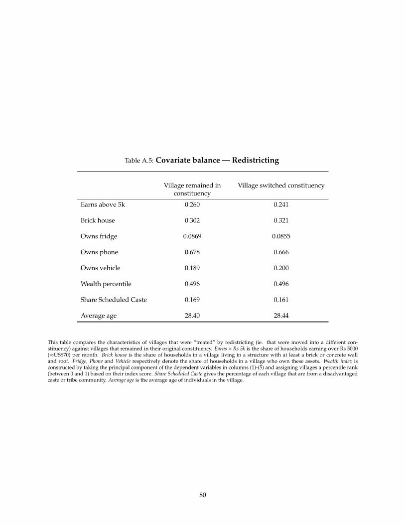
Table A.5: Covariate balance — Redistricting

Village remained inconstituency

Village switched constituency

Earns above 5k 0.260 0.241

Brick house 0.302 0.321

Owns fridge 0.0869 0.0855

Owns phone 0.678 0.666

Owns vehicle 0.189 0.200

Wealth percentile 0.496 0.496

Share Scheduled Caste 0.169 0.161

Average age 28.40 28.44

This table compares the characteristics of villages that were “treated” by redistricting (ie. that were moved into a different con-stituency) against villages that remained in their original constituency. Earns > Rs 5k is the share of households earning over Rs 5000(≈US$70) per month. Brick house is the share of households in a village living in a structure with at least a brick or concrete walland roof. Fridge, Phone and Vehicle respectively denote the share of households in a village who own these assets. Wealth index isconstructed by taking the principal component of the dependent variables in columns (1)-(5) and assigning villages a percentile rank(between 0 and 1) based on their index score. Share Scheduled Caste gives the percentage of each village that are from a disadvantagedcaste or tribe community. Average age is the average age of individuals in the village.

80

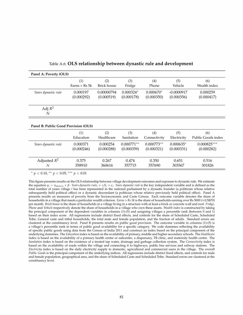
Table A.6: OLS relationship between dynastic rule and development

Panel A: Poverty (OLS)

(1) (2) (3) (4) (5) (6)Earns > Rs 5k Brick house Fridge Phone Vehicle Wealth index

Years dynastic rule 0.000197 0.00000794 0.000324∗ 0.000670∗ -0.0000917 0.000259(0.000292) (0.000519) (0.000178) (0.000350) (0.000356) (0.000417)

Adj R2

N

Panel B: Public Good Provision (OLS)

(1) (2) (3) (4) (5) (6)Education Healthcare Sanitation Connectivity Electricity Public Goods index

Years dynastic rule 0.000371 0.000254 0.000771∗∗ 0.000773∗∗ 0.000635∗ 0.000825∗∗∗

(0.000246) (0.000288) (0.000359) (0.000321) (0.000331) (0.000282)

Adjusted R2 0.375 0.267 0.474 0.350 0.651 0.516N 358910 360616 357715 357690 303567 301826

∗ p < 0.10, ∗∗ p < 0.05, ∗∗∗ p < 0.01

This figure presents results on the OLS relationship between village development outcomes and exposure to dynastic rule. We estimatethe equation yi = αdistrict + β · Years dynastic rulei + γXi + εi . Years dynastic rule is the key independent variable and is defined as thetotal number of years village i has been represented in the national parliament by a dynastic founder (a politician whose relativesubsequently held political office) or a dynastic descendant (a politician whose relative previously held political office). Panel Apresents results on measures of poverty from the Socioeconomic and Caste Census. Each outcome variable denotes the share ofhouseholds in a village that meets a particular wealth criterion. Earns > Rs 5k is the share of households earning over Rs 5000 (≈US$70)per month. Brick house is the share of households in a village living in a structure with at least a brick or concrete wall and roof. Fridge,Phone and Vehicle respectively denote the share of households in a village who own these assets. Wealth index is constructed by takingthe principal component of the dependent variables in columns (1)-(5) and assigning villages a percentile rank (between 0 and 1)based on their index score. All regressions include district fixed effects, and controls for the share of Scheduled Caste, ScheduledTribe, General caste and tribal households, the total male and female population, and the fraction of adults. Standard errors areclustered at the constituency level. Panel B presents results on public good provision. The outcome variable in columns (1)-(5) isa village’s percentile rank in terms of public good availability for a specific category. We code dummies reflecting the availabilityof specific public goods using data from the Census of India 2011 and construct an index based on the principal component of theunderlying dummies. The Education index is based on the availability of primary, middle and higher secondary schools. The Healthcareindex is based on the availability of a primary health centre or subcentre, a dispensary, TB clinic, and maternity health centre. TheSanitation index is based on the existence of a treated tap water, drainage and garbage collection system. The Connectivity index isbased on the availability of roads within the village and connecting it to highways, public bus services and railway stations. TheElectricity index is based on the daily electricity supply to domestic, agricultural and commercial users in the village. The overallPublic Goods is the principal component of the underlying indices. All regressions include district fixed effects, and controls for maleand female population, geographical area, and the share of Scheduled Caste and Scheduled Tribe. Standard errors are clustered at theconstituency level.

81

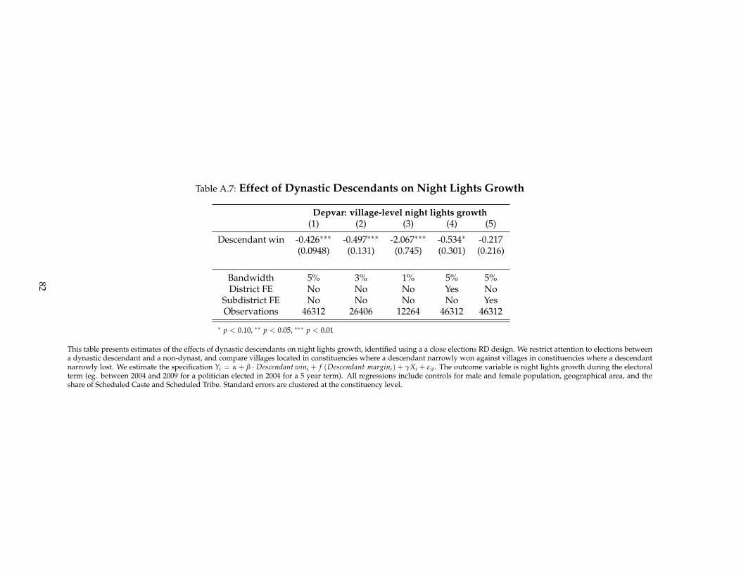
Table A.7: Effect of Dynastic Descendants on Night Lights Growth

Depvar: village-level night lights growth(1) (2) (3) (4) (5)

Descendant win -0.426∗∗∗ -0.497∗∗∗ -2.067∗∗∗ -0.534∗ -0.217(0.0948) (0.131) (0.745) (0.301) (0.216)

Bandwidth 5% 3% 1% 5% 5%District FE No No No Yes No

Subdistrict FE No No No No YesObservations 46312 26406 12264 46312 46312

∗ p < 0.10, ∗∗ p < 0.05, ∗∗∗ p < 0.01

This table presents estimates of the effects of dynastic descendants on night lights growth, identified using a a close elections RD design. We restrict attention to elections betweena dynastic descendant and a non-dynast, and compare villages located in constituencies where a descendant narrowly won against villages in constituencies where a descendantnarrowly lost. We estimate the specification Yi = α + β · Descendant wini + f (Descendant margini) + γXi + εit. The outcome variable is night lights growth during the electoralterm (eg. between 2004 and 2009 for a politician elected in 2004 for a 5 year term). All regressions include controls for male and female population, geographical area, and theshare of Scheduled Caste and Scheduled Tribe. Standard errors are clustered at the constituency level.

82

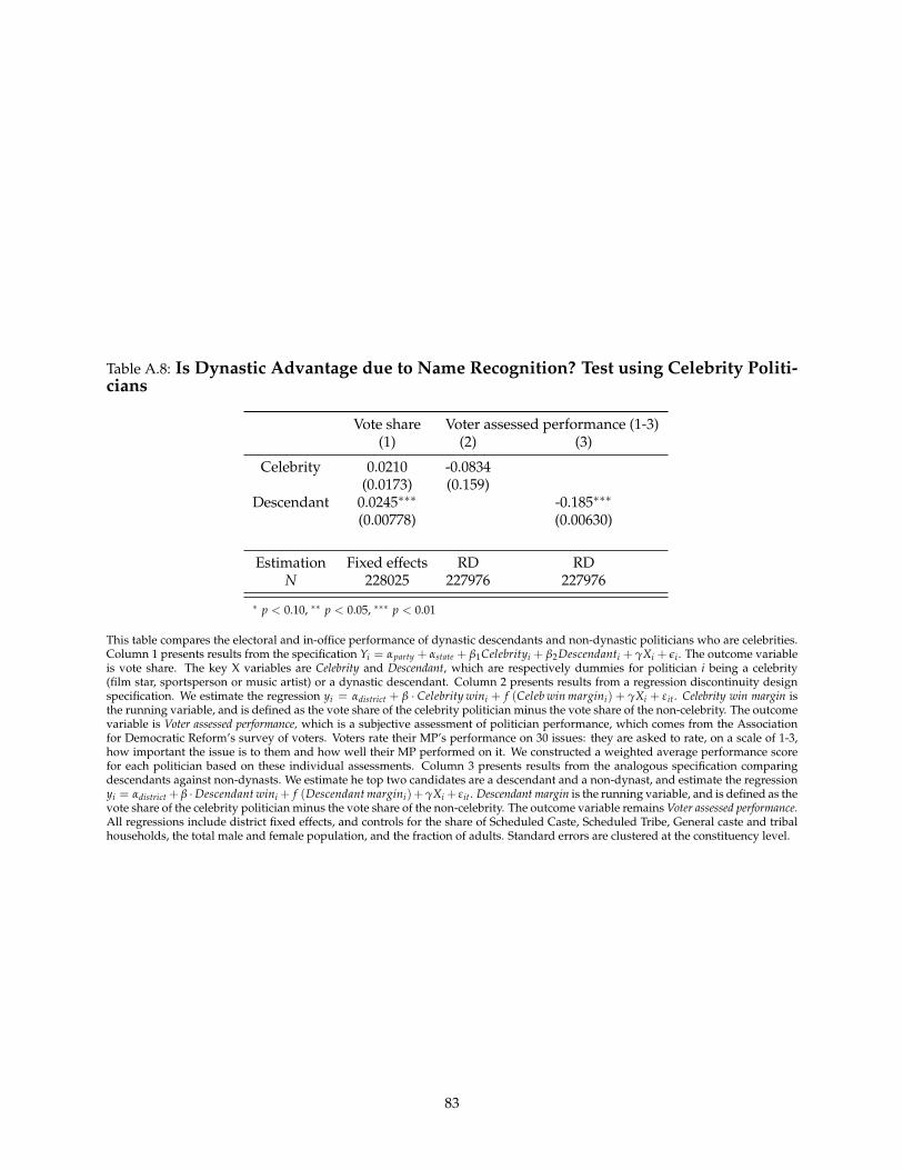
Table A.8: Is Dynastic Advantage due to Name Recognition? Test using Celebrity Politi-cians

Vote share Voter assessed performance (1-3)(1) (2) (3)

Celebrity 0.0210 -0.0834(0.0173) (0.159)

Descendant 0.0245∗∗∗ -0.185∗∗∗

(0.00778) (0.00630)

Estimation Fixed effects RD RDN 228025 227976 227976

∗ p < 0.10, ∗∗ p < 0.05, ∗∗∗ p < 0.01

This table compares the electoral and in-office performance of dynastic descendants and non-dynastic politicians who are celebrities.Column 1 presents results from the specification Yi = αparty + αstate + β1Celebrityi + β2Descendanti + γXi + εi . The outcome variableis vote share. The key X variables are Celebrity and Descendant, which are respectively dummies for politician i being a celebrity(film star, sportsperson or music artist) or a dynastic descendant. Column 2 presents results from a regression discontinuity designspecification. We estimate the regression yi = αdistrict + β · Celebrity wini + f (Celeb win margini) + γXi + εit. Celebrity win margin isthe running variable, and is defined as the vote share of the celebrity politician minus the vote share of the non-celebrity. The outcomevariable is Voter assessed performance, which is a subjective assessment of politician performance, which comes from the Associationfor Democratic Reform’s survey of voters. Voters rate their MP’s performance on 30 issues: they are asked to rate, on a scale of 1-3,how important the issue is to them and how well their MP performed on it. We constructed a weighted average performance scorefor each politician based on these individual assessments. Column 3 presents results from the analogous specification comparingdescendants against non-dynasts. We estimate he top two candidates are a descendant and a non-dynast, and estimate the regressionyi = αdistrict + β ·Descendant wini + f (Descendant margini)+γXi + εit. Descendant margin is the running variable, and is defined as thevote share of the celebrity politician minus the vote share of the non-celebrity. The outcome variable remains Voter assessed performance.All regressions include district fixed effects, and controls for the share of Scheduled Caste, Scheduled Tribe, General caste and tribalhouseholds, the total male and female population, and the fraction of adults. Standard errors are clustered at the constituency level.

83

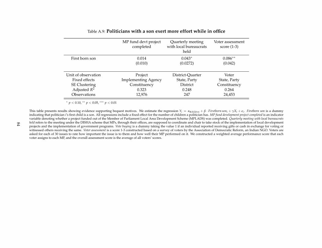
Table A.9: Politicians with a son exert more effort while in office

MP fund devt projectcompleted

Quarterly meetingwith local bureaucrats

held

Voter assessmentscore (1-3)

First born son 0.014 0.043∗ 0.086∗∗

(0.010) (0.0272) (0.042)

Unit of observation Project District-Quarter VoterFixed effects Implementing Agency State, Party State, Party

SE Clustering Constituency District ConstituencyAdjusted R2 0.323 0.248 0.264Observations 12,976 247 24,453

∗ p < 0.10, ∗∗ p < 0.05, ∗∗∗ p < 0.01

This table presents results showing evidence supporting bequest motives. We estimate the regression Yi = α#children + β · Firstborn soni + γXi + εi . Firstborn son is a dummyindicating that politician i’s first child is a son. All regressions include a fixed effect for the number of children a politician has. MP fund development project completed is an indicatorvariable denoting whether a project funded out of the Member of Parliament Local Area Development Scheme (MPLADS) was completed. Quarterly meeting with local bureaucratsheld refers to the meeting under the DISHA scheme that MPs, through their offices, are supposed to coordinate and chair to take stock of the implementation of local developmentprojects and the implementation of government programs. Vote buying is a dummy taking the value 1 if an individual reported receiving gifts or cash in exchange for voting orwitnessed others receiving the same. Voter assessment is a score 1-3 constructed based on a survey of voters by the Association of Democratic Reform, an Indian NGO. Voters areasked for each of 30 issues to rate how important the issue is to them and how well their MP performed on it. We constructed a weighted average performance score that eachvoter assigns to each MP, and the overall assessment score is the average of all voters’ scores.

84

85