[email protected] Washington State University · Fisher-Tippett-Gnedenko Theorem If F 2MDA(H), then...

High-Dimensional Extremes and Copulas

Haijun Li

[email protected] State University

CIAS-CUFE, Beijing, January 3, 2014

Figure : One-Period Binomial TreeHaijun Li High-Dimensional Extremes and Copulas CIAS-CUFE, Beijing, January 3, 2014 1 / 72

Outline

1 From Tukey to High-Dimensional Data Analysis

2 Univariate Extreme Value Theory: A Primer

3 Multivariate Extremes

4 Copula Representation of Multivariate Regular Variation

5 Tail Densities

6 Tail Densities of Vines

7 Concluding Remark

8 References

Haijun Li High-Dimensional Extremes and Copulas CIAS-CUFE, Beijing, January 3, 2014 2 / 72

John Wilder Tukey, 1915-2000

A chemist first and then a pure mathematician by training (PhDthesis “On Denumerability in Topology” in 1939)Statistician, information scientist, Presidential advisor...

Figure : From Paul Halmos’ “I Have a Photographic Memory”


Tukey’s Achievements

Teichmüller-Tukey Lemma, equivalent to the Axiom of Choice inaxiomatic set theoryTukey theory of analytic ideals, Tukey reducibility, ... (A competitorto Bourbaki’s approach to topology)

Computation: Fast Fourier TransformStatistics: Box plot, Quenouille-Tukey Jackknife...High-dimensional data analysis: Projection Pursuit (seekingnon-Gaussianity)


Tukey’s Collaborators and Awards

Focused on obtaining results rather than collecting credits.More than 100 collaborators and 55 PhD students. Worked wellwith Samuel Wilks, Walter Shewhart, Claude Shannon, John vonNeumann, Richard Feynman, etc.National Medal of Science, National Academy of Science, ForeignMember of the Royal Society, IEEE Medal of Honor, Samuel S.Wilks Memorial Award...


Tukey’s Belief

Much statistical methodology placed too great an emphasis onconfirmatory data analysis rather than exploratory data analysis.(Also see Leo Breiman, “Statistical Modeling: The Two Cultures”,Statistical Science, 2001)People should often start with their data and then look for atheorem, rather than vice versa.

Future of Data Analysis (Tukey, 1962)Data Analysis VS Mathematical Statistics? ... “All in all, I have come tofeel that my central interest is in data analysis ...”


New York Times Obituary (July 28, 2000):John Tukey, 85, Statistician; Coined the Word ‘Software’

A respected mathematician turned his back on mathematical proof,focusing on analyzing data instead.

“He legitimized that, because he wasn’t doing it because he wasn’tgood at math,’ Mr. Wainer (a Tukey’s former student) said. “He wasdoing it because it was the right thing to do.”

(David Donoho, High-Dimensional Data Analysis: The Blessings andCurses of Dimensionality, “Mathematical Challenges of the 21stCentury”, 2010)


Univariate Extremes

X1, . . . ,Xn are iid with df F .Mn := max{X1, . . . ,Xn} =: ∨n

i=1Xi .∧n

i=1Xi := min{X1, . . . ,Xn} = −max{−X1, . . . ,−Xn}, and so wefocus on large extremes only.

DefinitionIf there exist a non-degenerate df H, two normalizing sequences {cn}and {dn} with dn > 0, such that

limn→∞

P(

Mn − cn

dn≤ x

)= lim

n→∞F n(cn + dnx) = H(x), x ∈ R,

for all continuity points x of H, then F is said to be in the maximumdomain of attraction of H, and this is denoted as F ∈ MDA(H) orXn ∈ MDA(H).


Generalized Extreme Value Distribution (EV)

Fisher-Tippett-Gnedenko TheoremIf F ∈ MDA(H), then

H(x ; γ) = exp{−(1 + γx)−1/γ+ }, ∀x ∈ R,

where γ ∈ R is called the extreme value index.

After some location-scale transforms, we haveFréchet distribution: H+(x ; θ) = exp{−x−θ}, x > 0, θ > 0.Gumbel or double-exponential distribution: H0(x) = exp{−e−x},x ∈ R.(Reverse) Weibull distribution: H−(x ; θ) = exp{−(−x)θ}, x < 0,θ > 0.


Precise Tail Variations

xF := sup{x ∈ R : F (x) < 1}, the upper boundary of the support.F←(u) := inf{x ∈ R : F (x) ≥ u}, 0 < u < 1, the left-continuousinverse.

Gnedenko-de Haan Theorem: Fréchet MDA CaseF ∈ MDA(H(·; γ)) with γ > 0 if and only if xF =∞ and

limt→∞

1− F (tx)

1− F (t)= x−1/γ , x > 0,

where cn = 0 and dn = F←(1− n−1).


Precise Tail Variations (cont’d)

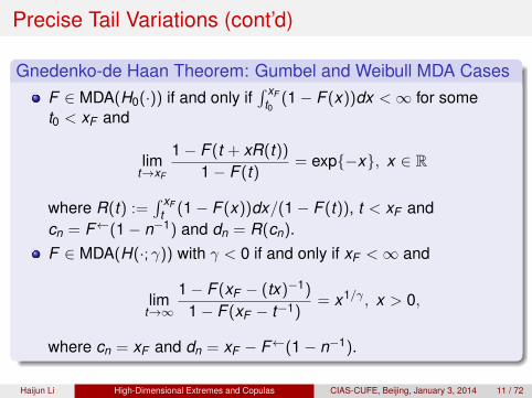
Gnedenko-de Haan Theorem: Gumbel and Weibull MDA CasesF ∈ MDA(H0(·)) if and only if

∫ xFt0

(1− F (x))dx <∞ for somet0 < xF and

limt→xF

1− F (t + xR(t))

1− F (t)= exp{−x}, x ∈ R

where R(t) :=∫ xF

t (1− F (x))dx/(1− F (t)), t < xF andcn = F←(1− n−1) and dn = R(cn).F ∈ MDA(H(·; γ)) with γ < 0 if and only if xF <∞ and

limt→∞

1− F (xF − (tx)−1)

1− F (xF − t−1)= x1/γ , x > 0,

where cn = xF and dn = xF − F←(1− n−1).


Example: Pareto Distribution

Consider the Pareto distribution

F (x) = 1− x−1/γ , x > 1, γ > 0.

Sincelim

t→∞1− F (tx)

1− F (t)= x−1/γ ,

F ∈ MDA(H(·; γ)) with Fréchet distribution H(·; γ), γ > 0.Set normalizing constants cn = 0 and dn = F−1(1− n−1) = nγ ,and clearly, for x > 0,

limn→∞

F n(cn + dnx) = limn→∞

(1− x−1/γ/n)n = exp{−x−1/γ}. �


Rewrite MDA in Terms of Tail Property

Without loss of generality, assume that X > 0.X ∼ F ∈ MDA(H)⇐⇒ limn→∞ F n(cn + dnx) = H(x).

Since − log x ≈ 1− x as x ↑ 1, it can be rephrased as follows

limn→∞

n(1− F (cn + dnx)) = − log H(x).

That is, X ∼ F ∈ MDA(H)⇐⇒ the tail dispersion stability:

limn→∞

n P(

X − cn

dn> x

)= − log H(x), ∀x > 0.


A Dimension-Free Tail Property of MDA

Define a (Radon) exponent measure

µ(x ,∞] := − log H(x), ∀ x ∈ R+.

Rewrite: ∀ “good” sets B ⊂ R+\{0}, µ(∂B) = 0,

limn→∞

n P(

X − cn

dn> x

)= − log H(x)

⇐⇒ limn→∞

n P(

X − cn

dn∈ B

)= µ(B)

︸︷︷︸Tail Dispersion

.

Note that the exponent measure µ(·) only has an asymptoticscaling property:

µ(t B) ≈ t−1/γµ(B), ∀ “good” sets B ⊂ R+\{0}, t →∞.


Scaling is Important for Prediction!

We want: µ(t B) = t−1/γµ(B), ∀ “good” sets B ⊂ R+\{0}, ∀ t > 0.

The tail stability and scaling allow us to estimate a tail regioncontaining fewer observations by a tail region containing moreobservations, whose distribution has the same shape.Extreme Value Theory = Mechanism for relating the probabilisticstructure within the range of the observed data to regions ofgreater extremity (Anderson, 1994).


Standardization of Regular Variation (RV)

DefinitionA random variable Z is regularly varying in the standard form if

limt→∞

t P(

Zt∈ B

)= ν(B), ∀ “good” sets B ⊂ R+\{0}, µ(∂B) = 0.

Note that ν(t B) = t−1ν(B) for any t > 0.

Consider two functions c(·),d(·) such that

c(tx)− c(t)d(t)

→ ψ(x) 6= 0, ∀x > 0, t →∞.

Observe thatTail Dispersion︷︸︸︷{c(Z )− c(t)

d(t)> x

}=

Standard RV︷︸︸︷{Zt> ψ←(x)

}


MDA⇔ Standard RV (Klüppelberg and Resnick, 2008)

Consider two functions c(·),d(·) such that

c(tx)− c(t)d(t)

→ ψ(x) 6= 0, ∀x > 0, t →∞.

1 If Z is standard regularly varying, then

X := c(Z ) ∈ MDA(H)

for some EV distribution H.2 If X ∈ MDA(H) for an EV distribution H(x), then there exists a

monotone transformation c(t) such that

Z := c←(X )

is standard regularly varying.


Remark

Regular variation is also the key ingredient in weak convergenceto stable laws (Meerschaert and Scheffler, 2001).Regular variation can be extended to general metric spaces todeal with functional data (Hult and Lindskog, 2006; Bingham andOstaszewski, 2008).“Extreme value distributions” for data clouds in high-dimensionalor functional spaces are difficult to define. Extremes emergingfrom high-dimensional data clouds may be best studied byexploring stability patterns of tail probability decays near databoundaries (Ledoux and Talagrand, 1991; Balkema andEmbrechts, 2007).Tail risk measures (e.g., Conditional Tail Expectation) can bederived directly from regular variation properties (see, e.g., Joeand Li, 2011).


von Mises Condition

Let df F have a positive derivative on [x0, xF ) for some 0 < x0 < xF ,and hF (x) = F ′(x)/(1− F (x)) be the hazard rate of F in a leftneighborhood of xF .

1 If there exist γ ∈ R and c > 0, such that

xF =

{∞ if γ ≥ 0−γ−1 if γ < 0

limx→xF

(1 + γx)hF (x) = c, (1)

then F ∈ MDA(H(·; γ/c)).2 If the derivative of F is monotone in a left neighborhood of xF for

some γ 6= 0, and if F ∈ MDA(H(·; γ/c)) for some c > 0, then Fsatisfies (1).


Examples

Consider the dfF (x) = 1− 1

log x, x > e,

that satisfies that

limx→∞

(x log x)hF (x) = 1.

Since the reciprocal hazard rate of this distribution is notasymptotically linear, there is no extreme value limit for F , withaffine thresholds.Note, however, that for the case where γ = 0, the von Misescondition is not necessary. For example, it is well known that thestandard normal df Φ ∈ MDA(H0(·)), but asymptoticallylimx→∞ x/hΦ(x) = 1. �


Laws of Small Numbers

Let {Z1, . . . ,Zn} be iid and standard regular varying:

n P (Z1 ∈ n B)→ ν(B), ∀ “good” sets B ⊂ R+\{0}, µ(∂B) = 0,

with scaling ν(t B) = t−1ν(B) for any t > 0.In particular, take B = (x ,∞) for x > 0, we have

limn→∞

n P (Z1 > nx) = ν((x ,∞)) =: ν.

Construct a counting process of exceedances of scaledobservations before time t :

Nn(t) =n∑

i=1

I{ in≤t , Zi>nx},

where IA denotes the indicator function of set A.


Dimension-Free Poisson Approximation

The count of exceedances before t :

Nn(t) =n∑

i=1

I{ in≤t , Zi>nx},

Take the expectation, we have

E(Nn(t)) = t × nP(Z1 > nx)→ tν, n→∞.

The counting processes (Nn(t), t ≥ 0) converge to a Poissonprocess with rate ν, as n→∞.The rate ν, or exponent measure ν(·) (also called the intensitymeasure for a good reason) encodes all the information ofextremes.


Multivariate Extremes

Xn = (X1,n, · · · ,Xd ,n), n = 1,2, · · · , are iid with df F (x1, . . . , xd ).Mn := (M1,n, . . . ,Md ,n), where Mi,n := ∨n

j=1Xi,j , 1 ≤ i ≤ d .

Notation: For any x , y ∈ Rd , the sum x + y , quotient x/y , and thevector inequalities are all operated component-wise.

Definition: Multivariate Extreme Value Distribution (MEV)If there exist a df G with non-degenerate margins, two normalizingsequences of real vectors {cn} and {dn} with dn > 0, such that

limn→∞

P(

Mn − cn

dn≤ x

)= lim

n→∞F n(cn + dnx) = G(x), x ∈ Rd ,

for all continuity points x of G, then F is said to be in the maximumdomain of attraction of G, and this is denoted as F ∈ MDA(G) orXn ∈ MDA(G).


Standardizing Margins⇒ Multivariate Scaling

Let X = (X1, . . . ,Xd ) ∼ F .

Xi ∼ Fi : the i-th marginal df of F .Gi : the i-th marginal df of G.Fi ∈ MDA(Gi), where Gi is the univariate, parametric EVdistribution.We assume that Fi is standard regularly varying.

Scaling Property Emerged from Equalizing Margins1 Gi is the standard Fréchet distribution with

log Gi(t xi) = t−1 log Gi(xi), ∀xi ∈ R+.

2 Jointly, the multivariate scaling emerges from the limiting process:

log G(t x) = t−1 log G(x), ∀x ∈ Rd+.


A Short Proof for Multivariate Scaling:

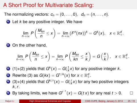
The normalizing vectors: cn = (0, . . . ,0), dn = (n, . . . ,n).

1 Let k be any positive integer. We have

limn→∞

P(

Mkn

n≤ x

)= lim

n→∞(F n(nx))k = Gk (x), x ∈ Rd

+.

2 On the other hand,

limn→∞

P(

Mkn

n≤ x

)= lim

n→∞P(

Mkn

kn≤ x

k

)= G

(xk

), x ∈ Rd

+.

3 (1)+(2) yields that Gk (x) = G( 1k x) for any positive integer k .

4 Rewrite (3) as G(kx) = G1/k (x) for x ∈ Rd+.

5 (3)+(4) yields that Gk/r (x) = G( rk x) for any two positive integers

k , r .6 By taking limits, we have Gt−1

(x) = G(t x) for any real t > 0. �Haijun Li High-Dimensional Extremes and Copulas CIAS-CUFE, Beijing, January 3, 2014 25 / 72

Remark on scaling G(t x) = Gt−1(x), t > 0

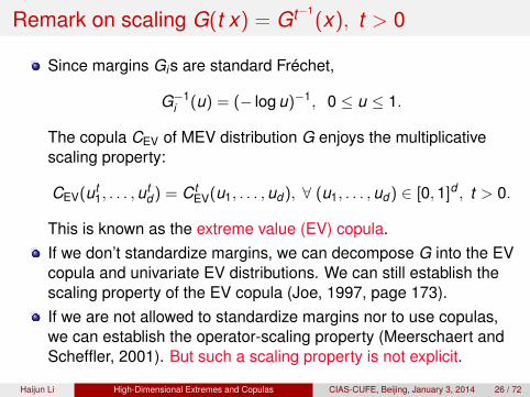
Since margins Gis are standard Fréchet,

G−1i (u) = (− log u)−1, 0 ≤ u ≤ 1.

The copula CEV of MEV distribution G enjoys the multiplicativescaling property:

CEV(ut1, . . . ,u

td ) = Ct

EV(u1, . . . ,ud ), ∀ (u1, . . . ,ud ) ∈ [0,1]d , t > 0.

This is known as the extreme value (EV) copula.If we don’t standardize margins, we can decompose G into the EVcopula and univariate EV distributions. We can still establish thescaling property of the EV copula (Joe, 1997, page 173).If we are not allowed to standardize margins nor to use copulas,we can establish the operator-scaling property (Meerschaert andScheffler, 2001). But such a scaling property is not explicit.


Multivariate Scaling⇒ Pickands Representation

The multivariate scaling property allows us to establish asemi-parametric representation for MEV G.

Let Sd−1+ = {a : a = (a1, . . . ,ad ) ∈ Rd

+, ||a|| = 1}, where || · || is a normdefined on Rd . Using the polar coordinates, G and its copula can beexpressed as follows:

G(x1, . . . , xd ) = exp

−b

∫

Sd−1+

∨

1≤i≤d

(ai

xi

)Q(da)

,

CEV(u1, . . . ,ud ) = exp

b

∫

Sd−1+

∧

1≤i≤d

(ai ln ui)Q(da)

,

where b > 0 and Q is a probability measure defined on Sd−1+ such that

b∫

Sd−1+

aiQ(da) = 1, 1 ≤ i ≤ d .


Pickands Representation⇒ Approximation Method

The probability measure Q is known as the spectral or angularmeasure. Its estimation and asymptotic properties can be found inResnick (2007).

Any probability measure Q on Sd−1+ can be approximated via

discrete probability measures on Sd−1+ .

The discretization of Q leads to a rich parametric family ofmax-stable multivariate Fréchet distributions (min-stablemultivariate exponential distributions, including the well-knownMarshall-Olkin distribution).The discretization of Q leads to a rich parametric family of EVcopulas with singularity components (e.g., Lévy-frailty copulas,Mai and Scherer, 2009).


Pickands Representation⇒ Positive Association

Y = (Y1, . . . ,Yd ) is said to positively associated if

E [f (Y )g(Y )] ≥ Ef (Y )Eg(Y ), ∀ f ,g : Rd → R, non-decreasing.

The positive association is a strong positive dependence and hasbeen extended to random elements in partially ordered, completeseparable metric space (Lindqvist, 1988).The positive association, equivalent to FKG inequality widely usedin statistical physics (Fortuin, Kastelyn, and Ginibre, 1971), is oneof several basic inequalities in analyzing concentrationphenomena (Ledoux and Talagrand, 1991).

Theorem (Marshall and Olkin, 1983)The MEV distribution G is positively associated.


Multivariate Regular Variation (MRV)

Assume that df F ∈ MDA(G).X = (X1, . . . ,Xd ) denote a random vector with distribution F andcontinuous, univariate margins F1, . . . ,Fd .Without loss of generality, margins F1, . . . ,Fd are identical.

Definition (Resnick, 1987 and 2007)The df F or X is said to be multivariate regularly varying at∞ withintensity measure ν if there exists a scaling function b(t)→∞ and anon-zero Radon measure ν(·) such that as t →∞,

t P(

Xb(t)

∈ B)→ ν(B), ∀ “good” sets B ⊂ Rd

+\{0}, with ν(∂B) = 0.

X is standard regularly varying if b(t) = t .


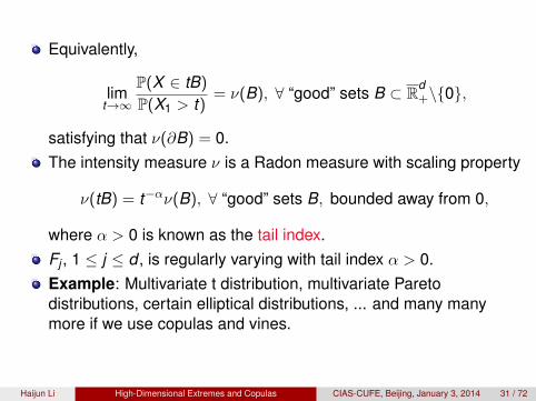
Equivalently,

limt→∞

P(X ∈ tB)

P(X1 > t)= ν(B), ∀ “good” sets B ⊂ Rd

+\{0},

satisfying that ν(∂B) = 0.The intensity measure ν is a Radon measure with scaling property

ν(tB) = t−αν(B), ∀ “good” sets B, bounded away from 0,

where α > 0 is known as the tail index.Fj , 1 ≤ j ≤ d , is regularly varying with tail index α > 0.Example: Multivariate t distribution, multivariate Paretodistributions, certain elliptical distributions, ... and many manymore if we use copulas and vines.


MDA⇔ Standard RV (Klüppelberg and Resnick, 2008)

Consider two functions c(t) = (c1(t), . . . , cd (t)), andd(t) = (d1(t), . . . ,dd (t)) such that component-wise

ci(txi)− ci(t)di(t)

→ ψi(x) 6= 0, ∀xi > 0, t →∞.

1 If Z = (Z1, . . . ,Zd ) is standard regularly varying, then

X = (c1(Z1), . . . , cd (Zd )) ∈ MDA(G)

for some MEV distribution G.2 If X ∈ MDA(G) for an MEV distribution G(x), then there exists a

component-wise monotone transformation c(t) such that

Z = (c←1 (X1), . . . , c←d (Xd ))

is standard regularly varying.


Example: Heavy-Tail Case

(Z1, . . . ,Zd ) is non-negative.For any α > 0, ci(z) := z1/α is increasing on R+, 1 ≤ i ≤ d .(X1, · · · ,Xd ) = (c1(Z1), . . . , cd (Z )) has the df F (x1, . . . , xd ).

Theorem (de Haan & Resnick, 1977; Marshall & Olkin, 1983)The following three statements are equivalent:

1 (Z1, . . . ,Zd ) is standard regular varying.2 (X1, · · · ,Xd ) is MRV with intensity measure ν(·).3 F ∈ MDA(G), where G(x) = exp{−ν([0, x ]c)}, x ∈ Rd

+, is ad-dimensional distribution with Fréchet margins

Gi(xi) = exp{−x−αi }, 1 ≤ i ≤ d .

Note that ν(tB) = t−αν(B) for any t > 0. �


The Copula Approach

Xn = (X1,n, · · · ,Xd ,n), n = 1,2, · · · , are iid with df F (x1, . . . , xd )that has continuous margins F1, . . . ,Fd .The copula of F :

C(u1, . . . ,ud ) := F (F−11 (u1), . . . ,F−1

d (u1)), (u1, . . . ,ud ) ∈ [0,1]d .

Figure : Two “squares” are topologically equivalent. Since limiting propertiesare topological, the copula method should be equivalent to the standard RVmethod.


Exponent and Tail Dependence Functions

(U1, . . . ,Ud ) := (F1(Xn,1), . . . ,Fd (Xn,d )).Define the exponent function: for all (w1, . . . ,wd ) ∈ Rd

+\{0},

a(w1, . . . ,wd ) := limu↓0

P(∪d

j=1 {Uj > 1− uwj})

u,

with scaling a(tw1, . . . , twd ) = t a(w1, . . . ,wd ) for t > 0.Define the tail dependence function:

b(w1, . . . ,wd ) := limu↓0

P(∩d

j=1 {Uj > 1− uwj})

u,

with scaling b(tw1, . . . , twd ) = tb(w1, . . . ,wd ) for t > 0.The existence of the exponent function ensures the existence ofthe exponent and tail dependence functions of all multivariatemargins of F .


Various tail dependence parameters are associated with thefunction b(·); for example, b(1, . . . ,1) is known as the taildependence coefficient.Due to the scaling property, b(·) = 0 iff b(1, . . . ,1) = 0, and in thiscase, the copula C is said to be (upper) tail independent.The notion of the exponent function a(·) can be traced back toGumbel (1960) and Pickands (1981). It describes the full extremaldependence structure of C, including the dependence of anymultivariate marginal tails.The tail dependence function b(·) is studied in Jaworski (2004,2006), Klüppelberg, Kuhn & Peng (2008), Nikoloulopoulos, Joe &Li (2009). Note that b(w1, . . . ,wd ) does not necessarily cover theextremal dependence structure of a multivariate margin.


Example: Archimedean Copulas

Let C(u;φ) = φ(∑d

i=1 φ−1(ui)) be an Archimedean copula where

the generator φ−1 is regularly varying at 1 with tail index β > 1.

a(w1, . . . ,wd ) =( d∑

j=1

wβj

)1/β, (w1, . . . ,wd ) ∈ Rd

+\{0}.

(Genest & Rivest, 1989; Barbe, Fougères & Genest, 2006)Let C have the survival copula C(u;φ) = φ(

∑di=1 φ

−1(ui)) withstrict generator φ−1, where φ is regularly varying at∞ with tailindex θ > 0.

b(w1, . . . ,wd ) =( d∑

j=1

w−1/θj

)−θ, (w1, . . . ,wd ) ∈ Rd

+\{0}.

(Charpentier & Segers, 2009) �


Tail Dependence Function “=” Intensity Measure

Theorem (Li and Sun, 2009)Let X = (X1, . . . ,Xd ) be a random vector with df F and copula C.

1 If F is MRV with intensity measure ν satisfying the scalingproperty that ν(tB) = t−αν(B), then for w = (w1, . . . ,wd ),

a(w) = ν(( d∏

i=1

[0,w−1/αi ]

)c), b(w) = ν

( d∏

i=1

(w−1/αi ,∞]

).

2 If the exponent function exists and marginal dfs F1, . . . ,Fd are(univariate) regularly varying, then

F (x1, . . . , xd ) = C(F1(x1), . . . ,Fd (xd )) is MRV.

The Radon measure generated by the exponent function a(·) is arescaled version of the intensity measure ν(·).


Copula Representation for MRV

Ingredients for High-Dimensional MRV1 Univariate dfs F1, . . . ,Fd are regularly varying with tail indexα1, . . . , αd respectively.

2 C is a copula with (upper) tail dependence limits.

Then F (x1, . . . , xd ) := C(F1(x1), . . . ,Fd (xd )) is MRV.

Remark:Tail dependence properties for vine copulas are obtained usingrecursive constructions according to underlying graph structures(Joe, Li and Nikoloulopoulos, 2010).


Copula Version of the Pickands Representation

Let C be a copula with (upper) exponent function a(·).The (upper) extreme-value copula of C:

CEV(u1, . . . ,ud ) = exp{−a(− log u1, . . . ,− log ud )},

where a(w1, . . . ,wd ) =∫Sd−1

+max1≤i≤d{aiwi}U(da), or

b(w1, . . . ,wd ) =

∫

Sd−11+

min1≤i≤d

{aiwi}U(da).

The spectral measure U(·) defined on Sd−11 is a finite measure.

In contrast to the Pickands representation for intensity measures,the spectral measure U(·) does not depend on margins.


Scaling Property, Again

Consider the d-dimensional copula C of a random vector (U1, . . . ,Ud )with standard uniform margins.

Recall that

a(tw) = ta(w), b(tw) = tb(w), ∀ w ∈ Rd+, t > 0.

The well-known Euler’s homogeneous theorem implies that

a(w) =d∑

j=1

∂a∂wj

wj , b(w) =d∑

j=1

∂b∂wj

wj , ∀w = (w1, . . . ,wd ) ∈ Rd+,

The partial derivatives can be interpreted as conditional limitingdistributions of the underlying copula C. For example,

∂b∂wj

= limu↓0

P(Ui > 1− uwi ,∀i 6= j | Uj = 1− uwj).


Deriving t-Copula via Euler’s Representation

Let X = (X1, . . . ,Xd ) have the t distribution Td ,ν,Σ with ν degreesof freedom and dispersion matrix Σ.The margins Fi = Tν for all 1 ≤ i ≤ d , where Tν is the t distributionfunction with ν degrees of freedom, and that Σ = (ρij) satisfiesρii = 1 for all 1 ≤ i ≤ d .The t-copula is defined as

Ct(u1, . . . ,ud ) = P(Tν(X1) ≤ u1, . . . ,Tν(Xd ) ≤ ud ).

Derive the extreme value copula Ct-EV.


Partial Correlation Matrix

For any i 6= j , k 6= j , let

ρi,k ;j =ρik − ρijρkj√

1− ρ2ij

√1− ρ2

kj

denote the partial correlations, and

Rj =

1 . . . ρ1,j−1;j ρ1,j+1;j . . . ρ1,d ;j...

. . ....

......

...ρ1,j−1;j . . . 1 ρj−1,j+1;j . . . ρj−1,d ;jρ1,j+1;j . . . ρj−1,j+1;j 1 . . . ρj+1,d ;j

......

......

. . ....

ρ1,d ;j . . . ρj−1,d ;j ρj+1,d ;j . . . 1

.


t-EV Copula

1 The tail dependence function of C is given by

b(w) =d∑

j=1

wjTd−1,ν+1,Rj

√ν + 1√1− ρ2

ij

[−(

wi

wj

)−1/ν

+ ρij

], i 6= j

,

for all w = (w1, . . . ,wd ) ∈ Rd+.

2 The t-EV copula is given by

Ct-EV(u1, . . . ,ud ) = exp{−a(w1, . . . ,wd )}, wj = − log uj , j = 1, . . . ,d ,

with exponent

a(w) =d∑

j=1

wjTd−1,ν+1,Rj

√ν + 1√1− ρ2

ij

[(wi

wj

)−1/ν

− ρij

], i 6= j

.


Two Limiting Distributions

Under some scaling conditions, Ct-EV(·) converges weakly to theHüsler-Reiss copula as ν →∞.As ν → 0, Ct-EV(·) converges weakly to a Marshall-Olkindistribution with some linear constraints.


The Tail Density Approach

The notion of tail density is local and geometric (Balkema andEmbrechts, 2007).Asymptotic analysis of tail risk measures often involves directlyintegral functionals of tail densities (Joe and Li, 2011).

Geometric Risk Analysis via Tail DensitiesA data cloud is a realization of a random set (e.g., random vectors,spatial point processes, high-dimensional Brownian motion, ...).“Central limit theorems” are concerned with clustering behaviorsat the “center” of a data cloud.“Extreme value theorems” are concerned with dispersive stabilitypatterns at the boundaries of a data cloud.Tail risk lives along the boundaries; it could be on the northeastboundary (max domain of attraction) or could be on the southwestboundary (min domain of attraction), or could be in other parts ofboundaries.


MRV Tail Densities

X = (X1, . . . ,Xd ) ∼ F that has identical continuous marginsF1, . . . ,Fd .F 1(t) := 1− F1(t) denotes the survival function of F1.

Theorem (de Haan and Resnick, 1987)

Assume the density f of F exists. If f (tx)

t−d F 1(t)→ λ(x) > 0 on Rd

+\{0}and uniformly on {x > 0 | ||x || = 1}, as t →∞, then

limt→∞

1− F (tx)

F 1(t)=

∫

[0,x ]cλ(y)dy =: µ([0, x ]c), x ∈ Rd

+\{0},

that is, F is MRV with intensity measure µ(·).


Perspective Shot of MTCJ Copula Density

Consider a bivariate MTCJ copula C(x , y) = (x−θ + y−θ − 1)−1/θ withdensity c(x , y) = (1 + θ)(xy)−θ−1(x−θ + y−θ − 1)−2−1/θ, θ > 0.Approaching the origin along the ray passing though (w1,w2), w1 > 0and w2 > 0, we have, as u → 0,

c(uw1,uw2) ≈ u−1[(1 + θ)(w1w2)−θ−1(w−θ1 + w−θ2 )−2−1/θ

︸︷︷︸?

]

0

1

0

1

0.133 4.151

2*(x^-1+y^-1-1)^-3*(x*y)^-2

Auto

Auto

15

x

z

xmin

zmin

xmax

zmax


Idea: Let (U1, . . . ,Ud )d∼ C. When u is sufficiently small,

tail density ≈ P(1− uwi ≤ Ui ≤ 1− u(wi − dwi),1 ≤ i ≤ d)/uκ

dw1 · · · dwd

≈ ud−κP(1− uwi ≤ Ui ≤ 1− uwi + d(uwi),1 ≤ i ≤ d)

d(uw1) · · · d(uwd )

In what follows, κ = 1.

0 1

0 1 1 - uw2 + udw2

1 - uw2

1 - uw1 1 - uw1 + udw1


Tail Densities of a Copula C

Assume that all the necessary regularity conditions hold.

DefinitionThe upper and lower tail densities of C are defined as

λU(w) := limu→0

DwC(1− uw1, . . . ,1− uwd )

u,

λL(w) := limu→0

DwC(uw1, . . . ,uwd )

u, ∀ w = (w1, . . . ,wd ) ∈ Rd

+

where Dw denotes the d-order partial differentiation operator and C isthe survival function of C.

C is upper (lower) tail independent if and only if λU = 0 (λL = 0).


Properties

Let c denote the density of C, then

λU(w) = limu→0

ud−1c(1− uwi ,1 ≤ i ≤ d),

λL(w) = limu→0

ud−1c(uwi ,1 ≤ i ≤ d), ∀ w = (w1, . . . ,wd ) ∈ Rd+

For a d-dimensional copula C, the tail densities are homogeneousof order 1− d . That is, λU(tw) = t1−dλU(w) for any w ∈ Rd

+ andt > 0.The Euler’s homogeneous theorem implies that the tail densitiesare directionally decreasing and convex, and go down to zero atinfinity.


Relation with Tail Dependence Functions

Recall that exponent and tail dependence functions:

a(w) := limu→0

P(Ui > 1− uwi , for some i)u

, ∀ w = (w1, . . . ,wd ) ∈ Rd+.

b(w) := limu→0

P(Ui > 1− uwi , for all i)u

, ∀ w = (w1, . . . ,wd ) ∈ Rd+.

TheoremRecall that Dw is the d-order partial differentiation operator.

λU(w) = Dwb(w) = (−1)d−1Dwa(w)

for all w ∈ Rd+.


Relation with Tail Density of MRV

Recall that λ(·) denotes the tail density of an MRV df F such that

limt→∞

1− F (tx)

F 1(t)=

∫

[0,x ]cλ(y)dy , x ∈ Rd

+.

Once again, λU denotes the upper tail density of the copula C of F .

Theorem (Li and Wu, 2013)Let α denote the tail index of F , then

λ(w1, . . . ,wd ) = αd (w1 · · ·wd )−α−1λU(w−α1 , . . . ,w−αd )

= |J(w−α1 , . . . ,w−αd )|λU(w−α1 , . . . ,w−αd ),

where |J(w−α1 , . . . ,w−αd )| is the Jacobian determinant of thehomeomorphism yi = w−αi , 1 ≤ i ≤ d .


Archimedean Tail Densities

Let C(u;φ) = φ(∑d

i=1 φ−1(ui)) be an Archimedean copula where the

Laplace transform φ.

Lower Tail DensityIf φ is regularly varying at∞ with tail index θ > 0, then

λL(w) =d∏

i=1

(1 +

i − 1θ

)( d∏

i=1

wi

)−1−1/θ( d∑

i=1

w−1/θi

)−θ−d.

Upper Tail Density

If φ−1 is regularly varying at 1 with tail index β > 1, then

λU(w) =d∏

i=1

((i − 1)β − 1)( d∏

i=1

wi

)β−1( d∑

i=1

wβi

)−d−1/β.


Lower Archimedean Tail Density

Figure 2: graphs for lower tail case

Its graph is shown below (θ = 1).

�

Theorem 2.5. Let X = (X1, . . . , Xd) be a non-negative MRV random vector with intensity

measure µ, copula C and continuous margins F1, . . . , Fd. If the marigins are tail equivalent

(i.e. Fi(t)/Fi(t)→ 1 as t→∞ for any i 6= j) with heavy-tail index β 0, then the upper tail

dependence function λ∗(·) exists and

1. λ∗(w) = ∂d

∂wµ([w

− 1β ,∞])

µ([1,∞]×Rd−1+ )

and a∗(w) = µ(([0,w− 1β ])c)

µ(([0,1]×Rd−1+ )c)

;

2. ∂d

∂w1···∂wdµ([w,∞])µ([0,1]c)

= (−1)d

a∗(1)· βd ·∏d

i=1 w−β−1i λ∗(w−β)

3 Tail approximation via tail density

In this section, we derive the tail asymptotics for V aRp(||X||), as p→ 1, for any fixed norm

|| · || on Rd. The results discussed in [6] can be obtained by taking the l1−norm and the tail

dependence function of Archimedean copulas.

Consider a non-negative MRV random vector X = (X1, . . . , Xd) with intensity measure

µ, joint distribution F and margins F1, . . . , Fd that are tail equivalent with heavy-tail index

β > 0. Without loss of generality, we use F1 to define the following limit:

q||·||(β, λ∗) := lim

t→∞Pr{||X|| > t}

F1(t)

6


Upper Archimedean Tail Density

Figure 1: graphs for upper tail case

4. λ∗(∞,∞) = 0.

The graph of this bivariate Gumbel copula is as follows (δ = 2).

�

Example 2.4. Consider a bivariate Clayton copula C(u, v; θ) = (u−θ + v−θ − 1)−1θ , θ > 0.

We know that Clayton copula only has lower tail dependence, no upper tail dependence. Its

lower tail density function is given by the following steps:

The bivariate copula density function with parameter θ is

c(uwi, 1 ≤ i ≤ 2) = (1 + θ)u−1(w−θ1 + w−θ2 − uθ)−1θ−2(w1w2)−θ−1

Therefore the lower tail density function is

λ(w) = limu→0

u · c(uwi, 1 ≤ i ≤ 2)

= limu→0

u · (1 + θ)u−1(w−θ1 + w−θ2 − uθ)−1θ−2(w1w2)−θ−1

= (1 + θ)(w1w2)−θ−1(w−θ1 + w−θ2 )−1θ−2, θ > 0.

The expression of λ(w) implies some properties:

1. λ(0, w2) = d(w1, 0) =∞

2. λ(0, 0) =∞

3. λ(∞, w2) = d(w1,∞) = 0

4. λ(∞,∞) = 0.

5


t Tail Density

Consider a d-dimensional symmetric t distribution with cdf

f (x ; ν,Σ) =Γ(ν+d

2 )

Γ(ν2 )(νπ)d/2 |Σ|− 1

2

[1 +

1ν

(xT Σ−1x)]− ν+d

2, x ∈ Rd

where ν > 0 is the degree of freedom, and Σ is a d × d dispersionmatrix.

Tail Density of t-Copula

λU(w) = λL(w) = π−d−1

2 |Σ|− 12 ν1−d Γ(ν+d

2 )

Γ(ν+12 )︸︷︷︸

ζ

[(w−1ν )T Σ−1w−

1ν ]−

ν+d2

∏di=1 w

ν+1ν

i

.

for any w ∈ Rd+.


Rewrite It as a Norm-Based Tail Density

Define a norm ||w || := (wT Σ−1w)1/2, w ∈ Rd+.

Let |J(w−1/ν1 , . . . ,w−1/ν

d )| be the Jacobian determinant oftopologically invariant transform yi = w−1/ν

i , 1 ≤ i ≤ d .Rewrite the upper tail density of a t copula:

λU(w1, . . . ,wd ) = ζ

d∏

i=1

w− ν+1

νi ((w−1/ν)T Σ−1w−1/ν)−

ν+d2

= ζνd |J(w−1/ν1 , . . . ,w−1/ν

d )| × ||w−1/ν ||−ν−d

For the symmetric t distribution itself,

λ(w1, . . . ,wd ) = ζνd ||w ||−ν−d

(de Haan and Resnick, 1987).


Vine Copula C of (U1, . . . ,Ud)

For any u = (u1, . . . ,ud ) ∈ [0,1]d , define

uS = (ui , i ∈ S), ∀ S ⊆ {1, . . . ,d}.

Ingredients for Vines{ci,j ,1 ≤ i < j ≤ d} = A set of the densities of bivariate linkingcopulas.For any S ⊆ {1, . . . ,d}, define the S-marginal densitycS := cS(uS).Define the conditional distribution of Uk given US = uS

Ck |S := Ck |S(uk |uS), k /∈ S.


D-Vine C

The density c{1,...,d} of C is constructed recursively as follows.

D-Vine Construction (Bedford and Cooke, 2001 and 2002)1 Baseline: For any 1 ≤ i ≤ d − 1, the density of the {i , i + 1}

margin is ci,i+1.2 Recursion:

c{1,...,d}c{2,...,d−1}

= c1,d(C1|2,...,d−1,Cd |2,...,d−1

) c{1,...,d−1}c{2,...,d−1}

c{2,...,d}c{2,...,d−1}

.


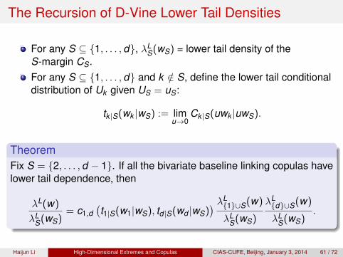
The Recursion of D-Vine Lower Tail Densities

For any S ⊆ {1, . . . ,d}, λLS(wS) = lower tail density of the

S-margin CS.For any S ⊆ {1, . . . ,d} and k /∈ S, define the lower tail conditionaldistribution of Uk given US = uS:

tk |S(wk |wS) := limu→0

Ck |S(uwk |uwS).

TheoremFix S = {2, . . . ,d − 1}. If all the bivariate baseline linking copulas havelower tail dependence, then

λL(w)

λLS(wS)

= c1,d(t1|S(w1|wS), td |S(wd |wS)

) λL{1}∪S(w)

λLS(wS)

λL{d}∪S(w)

λLS(wS)

.


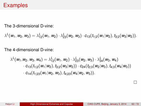
Examples

The 3-dimensional D-vine:

λL(w1,w2,w3) = λL12(w1,w2) · λL

23(w2,w3) · c13(t1|2(w1|w2), t3|2(w3|w2)).

The 4-dimensional D-vine:

λL(w1,w2,w3,w4) = λL12(w1,w2) · λL

23(w2,w3) · λL34(w3,w4)

· c13(t1|2(w1|w2), t3|2(w3|w2)) · c24(t2|3(w2|w3), t4|3(w4|w3))

· c14(t1|23(w1|w2,w3), t4|23(w4|w2,w3)).

�


Cautionary Remark

What happens if some or all bivariate baseline linking copulas of aD-vine C are tail independent? Joe et al (2010) has a partial answer:

C must be tail independent, e.g.,

C(uwi ,1 ≤ i ≤ d) ∼ uκh(w), as u → 0, κ > 1.

Some margins of C can still be tail dependent.

But can we quantify the order of scaling, e.g., κ, in the case of tailindependence of a vine copula?


Seeking Recursions of RV Near Data Boundaries

Consider the 3-dimensional D-vine

c(uw1,uw2,uw3) = c12(uw1,uw2) · c23(uw2,uw3)

· c13(C1|2(uw1|uw2),C3|2(uw3|uw2)), when u is small.

As functions of u, the regular variations of constructs c12, c23, C1|2,C3|2, and c13 should yield the regular varying property of c.

Example: If the baseline linking copulas C12 and C23 are Morgensterncopulas, and the linking copula C13 is a t copula, then c12(uw1,uw2)and c23(uw2,uw3) are asymptotically constant as u → 0 and

C1|2(uw1|uw2) ∼ uh1|2(w1,w2),C3|2(uw3|uw2) ∼ uh3|2(w2,w3), as u → 0.

Thus, as u → 0,

c(uw1,uw2,uw3) ∼ u−1h(w1,w2,w3).

That is, κ = 2. �Haijun Li High-Dimensional Extremes and Copulas CIAS-CUFE, Beijing, January 3, 2014 64 / 72

Concluding Remark: Predictability vs. Interpretability

In analyzing extremes, the goal is to develop accurate predictionrather than to provide good interpretability.In analyzing high-dimensional data clouds, margins are of multiplescales and it is entirely possible that only some multivariatemargins converge under possibly different surface/hyperplanethresholdings (Balkema and Embrechts, 2007).“Occam’s Razor” is often of little use in high-dimensionaldependence analysis. Simple and interpretable models do notmake the most accurate predictions. Sophisticated and flexiblemodels are called for.


If all a man has is a hammer, ...

Leo Breiman, “Statistical Modeling: The Two Cultures”, StatisticalScience (2001)

An old saying: “If all a man has is a hammer, then every problemlooks like a nail.”But the trouble for statisticians lately is that some of the newproblems have stopped looking like nails.Complex big data pose significant challenges.

Figure : One-Period Binomial TreeHaijun Li High-Dimensional Extremes and Copulas CIAS-CUFE, Beijing, January 3, 2014 66 / 72

References

Balkema, G. and Embrechts, P.: High Risk Scenarios andExtremes: A geometric approach. European Mathematical Society,Zürich, Switzerland, 2007.

Barbe, P., Fougères, A. L., Genest, C.: On the tail behavior ofsums of dependent risks. ASTIN Bulletin, 2006, 36(2):361-374.

Bedford, T. and Cooke, R. M.: Probability density decompositionfor conditionally dependent random variables modeled by vines.Annals of Mathematics and Artificial Intelligence, 2001,32:245-268.

Bedford, T. and Cooke, R. M.: Vines - a new graphical model fordependent random variables. The Annals of Statistics, 2002,30:1031-1068.

Charpentier, A. and Segers, J.: Tails of multivariate Archimedeancopulas. Journal of Multivariate Analysis, 2009, 100:1521-1537.


References

de Haan, L. and Resnick, S.I.: Limit theory for multivariate sampleextremes. Z. Wahrscheinlichkeitstheor. Verw. Gebiete, 1977,40:317-337.

de Haan, L. and Resnick, S.I.: On regular variation of probabilitydensities. Stochastic Process. Appl., 1987, 25:83-95.

Genest, C. and Rivest, L.-P.: A characterization of Gumbel’s familyof extreme value distributions. Statistics and Probability Letters,1989, 8:207-211.

Hua, L. and Joe, H.: Tail order and intermediate tail dependence ofmultivariate copulas. Journal of Multivariate Analysis, 2011,102:1454-1471.

Hua, L., Joe, H. and Li, H.: Relations between hidden regularvariation and tail order of copulas (under review). Technical report,Department of Mathematics, Washington State University, 2012.


References

Hüsler, J. and Reiss, R.-D.: Maxima of normal random vectors:between independence and complete dependence. Statistics &Probability Letters, 1989, 7(4):283–286.

Jaworski, P.: On uniform tail expansions of bivariate copulas.Applicationes Mathematicae, 2004, 31(4):397-415.

Jaworski, P.: On uniform tail expansions of multivariate copulasand wide convergence of measures. Applicationes Mathematicae,2006, 33(2):159-184.

Jaworski, P.: Tail Behaviour of Copulas, Chapter 8 in CopulaTheory and Its Applications, Eds. P. Jaworski, F. Durante, W.Härdle, and T. Rychlik, Lecture Notes in Statistics 198, Springer,New York, 2010.

Joe, H.: Multivariate Models and Dependence Concepts.Chapman & Hall, London, 1997.


References

Joe, H. and Li, H.: Tail risk of multivariate regular variation.Methodology and Computing in Applied Probability, 2011,13:671-693.

Joe, H., Li, H. and Nikoloulopoulos, A.K.: Tail dependencefunctions and vine copulas. Journal of Multivariate Analysis, 2010,101:252–270.

Klüppelberg, C., Kuhn, G. and Peng, L.: Semi-parametric modelsfor the multivariate tail dependence function – the asymptoticallydependent. Scandinavian Journal of Statistics, 2008,35(4):701–718.

Klüppelberg, C. and Resnick, S.: The Pareto copula, aggregationof risks, and the emperor’s socks. J. Appl. Probab., 2008, 45(1):67-84.

Kurowicka, D. and Cooke, R.: Uncertainty Analysis with HighDimensional Dependence Modelling. Wiley, New York, 2006.


References

Ledoux, M., and Talagrand, M.: Probability in Banach Spaces:Isoperimetry and Processes. Springer, 1991.

Li, H. and Sun, Y.: Tail dependence for heavy-tailed scale mixturesof multivariate distributions. J. Appl. Prob., 2009, 46 (4):925–937.

Li, H. and Wu, P.: Extremal dependence of copulas: A tail densityapproach. Journal of Multivariate Analysis, 2012, 114:99-111.

Marshall, A. W., and Olkin, I.: Domains of attraction of multivariateextreme value distributions. Annuals of Probability, 1983,11:168-177.

Meerschaert, M. M. and Scheffler, H.-P.: Limit Distributions forSums of Independent Random Vectors. John Wiley & Sons, 2001.


References

Mai, J.-F. and Scherer, M.: Reparameterizing Marshall-Olkincopulas with applications to sampling. Journal of StatisticalComputation & Simulation, 2009, 1-23.

Nikoloulopoulos, A. K., Joe, H. and Li, H.: Extreme valueproperties of multivariate t copulas. Extremes, 2009, 12:129–148.

Resnick, S.: Extreme Values, Regularly Variation, and PointProcesses, Springer, New York, 1987.

Resnick, S.: Hidden regular variation, second order regularvariation and asymptotic independence. Extremes, 2002,5:303-336.

Resnick, S.: Heavy-Tail Phenomena: Probabilistic and StatisticalModeling. Springer, New York, 2007.


[email protected] Washington State University · Fisher-Tippett-Gnedenko Theorem If F 2MDA(H), then...

Documents

Transcript of [email protected] Washington State University · Fisher-Tippett-Gnedenko Theorem If F 2MDA(H), then...