Light propagates in the form of waves
60
WAVE OPTICS (FOURIER OPTICS) ARNAUD DUBOIS October 2012
Transcript of Light propagates in the form of waves

WAVE OPTICS
(FOURIER OPTICS)
ARNAUD DUBOIS
October 2012
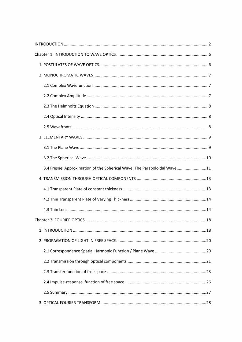
INTRODUCTION ............................................................................................................................... 2
Chapter 1: INTRODUCTION TO WAVE OPTICS ................................................................................. 6
1. POSTULATES OF WAVE OPTICS................................................................................................ 6
2. MONOCHROMATIC WAVES ..................................................................................................... 7
2.1 Complex Wavefunction ..................................................................................................... 7
2.2 Complex Amplitude ........................................................................................................... 7
2.3 The Helmholtz Equation .................................................................................................... 8
2.4 Optical Intensity ................................................................................................................ 8
2.5 Wavefronts ........................................................................................................................ 8
3. ELEMENTARY WAVES .............................................................................................................. 9
3.1 The Plane Wave ................................................................................................................. 9
3.2 The Spherical Wave ......................................................................................................... 10
3.4 Fresnel Approximation of the Spherical Wave; The Paraboloidal Wave.......................... 11
4. TRANSMISSION THROUGH OPTICAL COMPONENTS ............................................................. 13
4.1 Transparent Plate of constant thickness ......................................................................... 13
4.2 Thin Transparent Plate of Varying Thickness ................................................................... 14
4.3 Thin Lens ......................................................................................................................... 14
Chapter 2: FOURIER OPTICS .......................................................................................................... 18
1. INTRODUCTION ..................................................................................................................... 18
2. PROPAGATION OF LIGHT IN FREE SPACE ............................................................................... 20
2.1 Correspondence Spatial Harmonic Function / Plane Wave ............................................. 20
2.2 Transmission through optical components ..................................................................... 21
2.3 Transfer function of free space ....................................................................................... 23
2.4 Impulse-response function of free space ....................................................................... 26
2.5 Summary ......................................................................................................................... 27
3. OPTICAL FOURIER TRANSFORM ............................................................................................ 28
3.1 Amplitude in the far-field ................................................................................................ 28
3.2 Amplitude in the back focal plane of a lens ..................................................................... 29
4. DIFFRACTION ......................................................................................................................... 32
4.1 Fresnel diffraction ........................................................................................................... 32
4.2 Fraunhofer diffraction ..................................................................................................... 34
5. SPATIAL FILTERING ................................................................................................................ 36
6. Image formation .................................................................................................................... 39
6.1 Impulse response function .............................................................................................. 40
6.2 Image formation with coherent illumination .................................................................. 41
6.3 Image formation with incoherent illumination ............................................................... 41
Chapter 3: COHERENCE ................................................................................................................. 46
1. Statistical properties of random light .................................................................................... 46
1.1 Optical intensity .............................................................................................................. 46
1.2 Temporal coherence and spectrum ................................................................................. 48
1.3 Spatial coherence ............................................................................................................ 50
1.4 Gain of spatial coherence by propagation: Zernike and Van Cittert theorem ................. 52
2. Interference of partially coherent light ................................................................................. 54
2.1 Interference and temporal coherence ............................................................................ 54
2.2 Interference and spatial coherence ................................................................................. 55

1
References
1. “Fundamentals of Photonics” (Wiley Series in Pure and Applied Optics). Bahaa E. A. Saleh, Malvin Carl Teich. John Wiley & Sons, 1st edition (August 15, 1991)
2. “Introduction to Fourier Optics”, J.W. Goodman (Stanford University). Second edition Mc Graw-Hill (1996)
3. “Principle of Optics”, Born and Wolf (Pergamon Press 6th edition)

2
INTRODUCTION
Light is an electromagnetic wave phenomenon. Electromagnetic radiations are classified in
different categories, depending on their frequency. Light occupies a limited region of the
electromagnetic spectrum. The range of optical wavelengths contains three bands: ultraviolet
(10 to 390 nm), visible (390 to 760 nm), and infrared (760 nm to 1 mm). The corresponding range
of optical frequencies stretches from 3 1011 Hz to 3 1016 Hz.
The spectrum of electromagnetic waves
3
Since light is an electromagnetic wave, light can be described by the same theoretical
principles that govern all forms of electromagnetic radiation. Electromagnetic radiation
propagates in the form of two coupled vector waves, an electric-field wave and a magnetic-field
wave.
Although light is described by two wave vectors, it is possible to describe many optical
phenomena using a scalar wave theory. In this theory, light is described by a single scalar
wavefunction. This approximate way of treating light is called scalar wave optics, or simply wave
optics.
When light waves propagate through and around objects whose dimensions are much
greater than the wavelength, the wave nature of light is not discernable. In that case, the
behaviour of light can be described by rays. This model of light, called ray optics, obeys a set of
geometrical rules. Theoretically, ray optics is the limit of wave optics when the wavelength is
zero. However, the wavelength needs not actually be equal to zero for the ray-optics theory to
be useful. As long as the light waves propagate through and around objects whose dimensions
are much greater than the wavelength, the ray theory suffices for describing most phenomena.
Because the wavelength of visible light is much shorter than the dimensions of the visible objects
encountered in our daily lives, manifestations of the wave nature of light are not apparent
without careful observation.
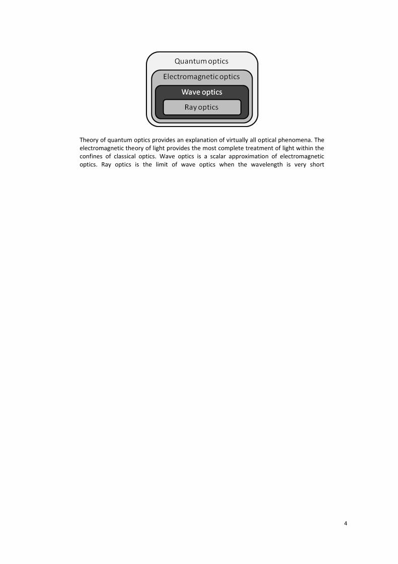
Thus, the electromagnetic theory of light encompasses wave optics, which in turn,
encompasses ray optics. Ray optics and wave optics provide approximate models of light which
derive their validity from their successes in producing results that approximate those based on
rigorous electromagnetic theory.
Although electromagnetic optics provides the most complete treatment of light within the
confines of classical optics, there are certain optical phenomena that are characteristically
quantum mechanical in nature and cannot be explained classically (spectrum of blackbody
radiation, absorption and emission of light by matter at specific wavelengths, etc...). These
phenomena are described by a quantum electromagnetic theory known as quantum
electrodynamics. For optical phenomena, this theory is also referred to as quantum optics.
Historically, optical theory developed roughly in the following sequence: (1) ray optics; (2)
wave optics; (3) electromagnetic optics; (4) quantum optics. Not surprisingly, these models are
progressively more difficult and sophisticated, having being developed to provide explanations
for the outcomes of successively more complex and precise optical experiments.
4
Theory of quantum optics provides an explanation of virtually all optical phenomena. The electromagnetic theory of light provides the most complete treatment of light within the confines of classical optics. Wave optics is a scalar approximation of electromagnetic optics. Ray optics is the limit of wave optics when the wavelength is very short

5
6
Chapter 1: INTRODUCTION TO WAVE OPTICS
Wave optics is a scalar approximation of electromagnetic optics. The vectorial nature of light is
therefore ignored in the wave optics theory. Wave optics can be used for describing many
optical phenomena that cannot be described by ray optics, including interference and
diffraction. However, wave optics cannot describe optical phenomena that require a vector
formulation, such as polarization effects. The wave optics theory is also not capable of providing
a complete picture of reflection and refraction of light at the boundaries between dielectric
materials.
1. POSTULATES OF WAVE OPTICS
The theory of wave optics can be built from a set of postulates. These postulates can be justified
by the electromagnetic theory of light :
- Light propagates in the form of waves.
- In free space, light waves travel with speed c0.
- A homogeneous transparent medium (such as glass) is characterized by a single constant, its
refractive index ( 1)n . In a medium of refractive index n, light waves travel with a reduced
speed 0 /c c n .
- An optical wave is described mathematically by a real function of position ( , , )x y zr and time
t, denoted ( , )u tr and known as the wavefunction. It satisfies the wave equation:
22
2 2
10
uu
c t
where 2 is the Laplacian operator. It is a scalar differential operator. In Cartesian coordinates,
it is defined as 2 2 2
2
2 2 2
u u uu
x y z
.
Any function satisfying the wave equation represents a possible optical wave.
Because the wave equation is linear, the principle of superposition applies; i.e., if 1( , )u tr and
2( , )u tr represent optical waves, then 1 2( , ) ( , ) ( , )u t u t u t r r r also represents a possible optical
wave.

7
The wave equation is approximately applicable to media with position-dependent
refractive indices, provided that the variation is slow within distances of a wavelength. The
medium is then said to be locally homogeneous. For such media, n and c are simply replaced
by position-dependent functions ( )n r and ( )c r , respectively.
2. MONOCHROMATIC WAVES
In the wave optics theory, a monochromatic wave is represented by a wavefunction with
harmonic time dependence,
( , ) ( )cos 2 ( )u t a t r r r ,
where
( )a r = amplitude ( ) r = phase
= frequency (cycles/s or Hz) = 2 = angular frequency (radians/s).
Both the amplitude and the phase are generally position dependent, but the wavefunction is a
harmonic function of time with frequency at all positions. As seen in the introduction, the
frequency of optical waves lies in the range 3 1011 to 3 1016 Hz.
2.1 Complex Wavefunction
It is usual and convenient to represent the real wavefunction ( , )u tr in terms of a complex
function
( , ) ( )exp ( ) exp( 2 )U t a j j t r r r ,
so that
*( , ) Re ( , ) 1/2 ( , ) ( , )u t U t U t U t r r r r .
The function ( , )U tr , known as the complex wavefunction, describes the wave completely; the
wavefunction ( , )u tr is simply its real part. Like the wavefunction ( , )u tr , the complex
wavefunction ( , )U tr must also satisfy the wave equation
22
2 2
10
UU
c t
.
2.2 Complex Amplitude
The complex wavefunction can be written in the form
8
( , ) ( )exp( 2 )U t U j tr r ,
where the time-independent factor ( ) ( )exp ( )U a jr r r is referred to as the complex
amplitude. The wavefunction ( , )u tr is therefore related to the complex amplitude by
( , ) Re ( )exp( 2 )u t U j tr r
At a given position r , the complex amplitude ( )U r is a complex variable whose magnitude
( ) ( )U ar r is the amplitude of the wave and whose argument arg ( ) ( )U r r is the phase.
2.3 The Helmholtz Equation
The monochromatic wave must satisfy the wave equation. Substituting
( , ) ( )exp( 2 )U t U j tr r into the wave equation, we obtain the differential equation
2 2 ( ) 0k U r
called the Helmholtz equation, where
2 / /k c c
is referred to as the wavenumber.
2.4 Optical Intensity
The optical intensity of a monochromatic ware is defined as the absolute square of its complex
amplitude
2( ) ( )I r U r
The intensity of a monochromatic wave does not vary with time.
2.5 Wavefronts
The wavefronts are the surfaces of equal phase, ( ) r = constant. The constants are often taken
to be multiples of 2, ( ) 2 q r , where q is an integer.
9
Summary
• A monochromatic wave of frequency is described by a complex wavefunction
( , ) ( )exp( 2 )U t U j tr r , which satisfies the wave equation.
• The complex amplitude ( )U r satisfies the Helmholtz equation; its magnitude ( )U r and
argument arg ( )U r are the amplitude and phase of the wave, respectively. The optical
intensity is 2
( ) ( )I r U r . The wavefronts are the surfaces of constant phase,
( ) arg ( ) 2U q r r ( q = integer).
• The wavefunction ( , )u tr is the real part of the complex wavefunction, ( , ) Re ( , )u t U tr r .
The wavefunction also satisfies the wave equation.
3. ELEMENTARY WAVES
We consider here two special monochromatic waves: the plane wave and the spherical wave.
These waves are the simplest solutions to the Helmholtz equation in a homogeneous medium.
3.1 The Plane Wave
The plane wave has a complex amplitude
( ) exp . exp x y zU A j A j k x k y k z r k r ,
where A is a constant called the complex envelope, and , ,x y zk k kk is called the
wavevector.
For the plane wave to satisfy the Helmholtz equation, 2 2 2 2x y zk k k k , so that the magnitude
of the wavevector k is the wavenumber k .
Since the phase arg ( ) argU A r k r , the wavefronts obey
2 argx y zk x k y k z q A k r ( q = integer). This is the equation describing parallel
planes perpendicular to the wavevector k (hence the name "plane wave"). These planes are
separated by a distance 2 /k , so that
/c
where is called the wavelength.

10
The plane wave has a constant intensity 2
( )I r A everywhere in space so that it carries
infinite power. This wave is clearly an idealization since it exists everywhere and at all times.
If the z axis is taken in the direction of the wavevector k , then ( ) expU r A jkz and
the corresponding wavefunction is
( , ) cos 2 arg cos 2 / argu t A t kz A A t z c A r
The wavefunction is therefore periodic in time with period 1/ , and periodic in space with
period 2 /k , which is equal to the wavelength . Since the phase of the complex wavefunction,
arg ( , ) 2 / argU t t z c A r , varies with time and position as a function of the variable
/t z c (see Fig), c is called the phase velocity of the wave. ( , )u z t
A plane wave travelling in the z direction is a periodic function of z with spatial period
and a periodic function of t with temporal period 1/.
In a medium of refractive index n :
- the phase velocity is 0 /c c n
- the wavelength is 0/ /c c n , so that 0 /n where 0 0 /c is the
wavelength in free space. For a given frequency , the wavelength in the medium is
reduced relative to that in free space by the factor n.
- as a consequence, the wavenumber 2 /k increases relative to that in free space
( 0 02 /k ) by the factor n .
In summary: as a monochromatic wave propagates through media of different refractive
indices its frequency remains the same, but its velocity, wavelength, and wavenumber are
modified.
3.2 The Spherical Wave
Another simple solution of the Helmholtz equation is the spherical wave. The complex amplitude
of a spherical wave is
( / )expU A r jkr r
11
where r is the distance from the origin and 2 / /k c c is the wavenumber.
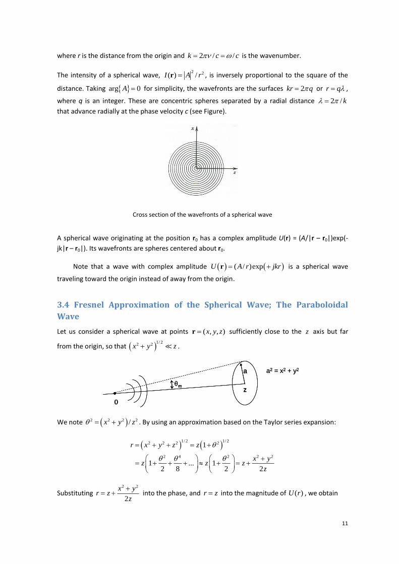
The intensity of a spherical wave, 2 2( ) /I A rr , is inversely proportional to the square of the
distance. Taking arg 0A for simplicity, the wavefronts are the surfaces 2kr q or r q ,
where q is an integer. These are concentric spheres separated by a radial distance 2 /k
that advance radially at the phase velocity c (see Figure).
Cross section of the wavefronts of a spherical wave
A spherical wave originating at the position r0 has a complex amplitude U(r) = (A/|r – r0|)exp(-
jk|r – r0|). Its wavefronts are spheres centered about r0.
Note that a wave with complex amplitude ( / )expU A r jkr r is a spherical wave
traveling toward the origin instead of away from the origin.
3.4 Fresnel Approximation of the Spherical Wave; The Paraboloidal
Wave
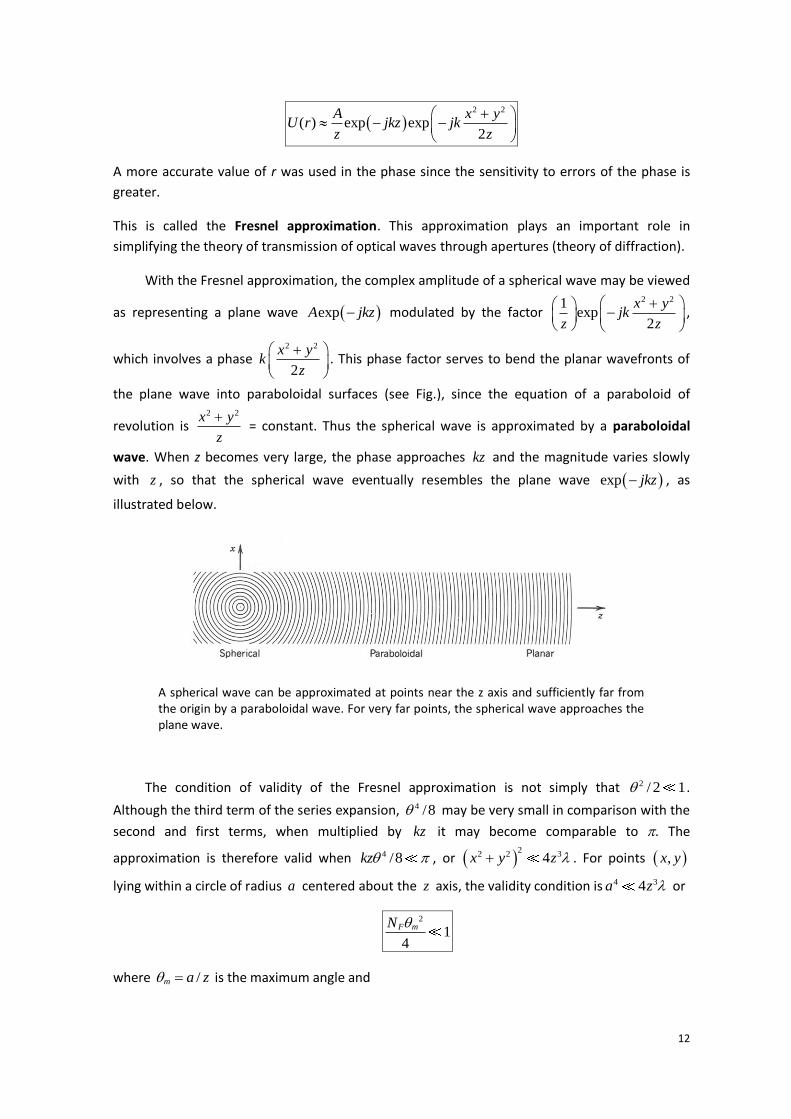
Let us consider a spherical wave at points ( , , )x y zr sufficiently close to the z axis but far
from the origin, so that 1/ 2
2 2x y z .
a
0
zm
a2 = x2 + y2a
0
zm
a
0
zm
a2 = x2 + y2
We note 2 2 2 2/x y z . By using an approximation based on the Taylor series expansion:
1/ 2 1/ 2
2 2 2 2
2 4 2 2 2
1
1 ... 12 8 2 2
r x y z z
x yz z z
z
Substituting 2 2
2
x yr z
z
into the phase, and r z into the magnitude of ( )U r , we obtain
12
2 2
( ) exp exp2
A x yU r jkz jk
z z
A more accurate value of r was used in the phase since the sensitivity to errors of the phase is
greater.
This is called the Fresnel approximation. This approximation plays an important role in
simplifying the theory of transmission of optical waves through apertures (theory of diffraction).
With the Fresnel approximation, the complex amplitude of a spherical wave may be viewed
as representing a plane wave expA jkz modulated by the factor 2 21
exp2
x yjk
z z
,
which involves a phase 2 2
2
x yk
z
. This phase factor serves to bend the planar wavefronts of
the plane wave into paraboloidal surfaces (see Fig.), since the equation of a paraboloid of
revolution is 2 2x y
z
= constant. Thus the spherical wave is approximated by a paraboloidal
wave. When z becomes very large, the phase approaches kz and the magnitude varies slowly
with z , so that the spherical wave eventually resembles the plane wave exp jkz , as
illustrated below.
A spherical wave can be approximated at points near the z axis and sufficiently far from the origin by a paraboloidal wave. For very far points, the spherical wave approaches the plane wave.
The condition of validity of the Fresnel approximation is not simply that 2 / 2 1 .
Although the third term of the series expansion, 4 /8 may be very small in comparison with the
second and first terms, when multiplied by kz it may become comparable to . The
approximation is therefore valid when 4 /8kz , or 2
2 2 34x y z . For points ,x y
lying within a circle of radius a centered about the z axis, the validity condition is 4 34a z or
2
14
F mN
where /m a z is the maximum angle and

13
2
F
aN
z
is known as the Fresnel number.
EXERCISE 1: Validity of the Fresnel Approximation.
Determine the radius of a circle within which a spherical wave of wavelength = 633 nm, originating at a
distance 1 m away, may be approximated by a paraboloidal wave. Determine the maximum angle m and
the Fresnel number NF.
4. TRANSMISSION THROUGH OPTICAL COMPONENTS
We now proceed to examine the transmission of optical waves through transparent optical
components such as plates and lenses. The effect of reflection at the surfaces of these
components will be ignored, since it cannot be properly described using the scalar wave optics
model of light. The effect of absorption in the material is also ignored. The main emphasis here
is on the phase shift introduced by these components and on the associated wavefront bending.
4.1 Transparent Plate of constant thickness
Consider first the transmission of a plane wave through a transparent plate of refractive index n
and thickness d surrounded by free space. The surfaces of the plate are the planes z = 0 and z =
d and the incident wave travels in the z direction. Let ( , , )U x y z be the complex amplitude of
the wave. Since external and internal reflections are ignored, ( , , )U x y z is assumed to be
continuous at the boundaries. The ratio ( , ) ( , , ) / ( , ,0)t x y U x y d U x y therefore represents the
complex amplitude transmittance of the plate. The incident plane wave continues to propagate
inside the plate as a plane wave with wavenumber 0nk , so that ( , , )U x y z is proportional to
0exp jnk d . Thus 0( , , ) / ( , ,0) expU x y d U x y jnk d , so that
0( , ) expt x y jnk d
i.e., the plate introduces a phase shift 0 2 /nk d d . z0 d
n
k
z0 d
n
k

14
4.2 Thin Transparent Plate of Varying Thickness
We consider now a thin transparent plate whose thickness ( , )d x y varies smoothly as a function
of x and y . The incident wave is a paraxial wave. The plate lies between the planes z = 0 and z =
d0, which are regarded as the boundaries of the optical component.
The wave crosses a thin plate of width ( , )d x y surrounded by thin layers of air of total
width 0 ( , )d d x y . The local transmittance is the product of the transmittances of a thin layer of
air of thickness 0 ( , )d d x y and a thin layer of material of thickness ( , )d x y so that
0 0 0( , ) exp ( , ) exp ( , )t x y jnk d x y jk d d x y , from which
0 0( , ) exp 1 ( , )t x y h j n k d x y
where 0 0 0exph jk d is a constant phase factor. This relation is valid in the paraxial
approximation (all angles are small) and when the thickness d0 is sufficiently small.
A transparent plate of varying thickness.
4.3 Thin Lens
The general expression for the complex amplitude transmittance of a thin transparent plate of
variable thickness is now applied to the plano-convex thin lens.
15
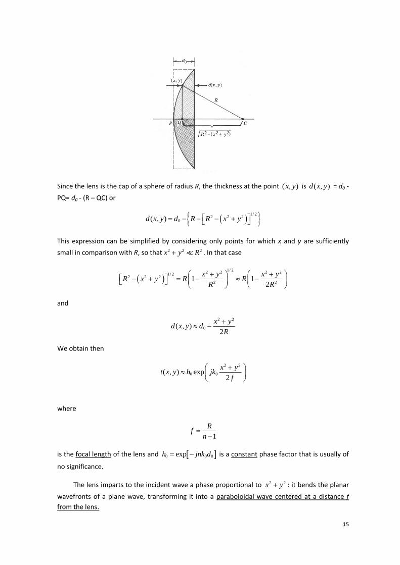
Since the lens is the cap of a sphere of radius R, the thickness at the point ( , )x y is ( , )d x y = d0 -
PQ= d0 - (R – QC) or
1/ 2
2 2 20( , )d x y d R R x y
This expression can be simplified by considering only points for which x and y are sufficiently
small in comparison with R, so that 2 2 2x y R . In that case
1/ 2
2 2 2 21/ 2
2 2 2
2 21 1
2
x y x yR x y R R
R R
and
2 2
0( , )2
x yd x y d
R
We obtain then
2 2
0 0( , ) exp2
x yt x y h jk
f
where
1
Rf
n
is the focal length of the lens and 0 0 0exph jnk d is a constant phase factor that is usually of
no significance.
The lens imparts to the incident wave a phase proportional to 2 2x y : it bends the planar
wavefronts of a plane wave, transforming it into a paraboloidal wave centered at a distance f
from the lens.
16
Double-Convex Lens: the complex amplitude transmittance of the double-convex lens is given by
2 2 2 2
0 0
1 2
( , ) exp ( 1) exp ( 1)2 2
x y x yt x y jk n jk n
R R
2 2
0 0( , ) exp2
x yt x y h jk
f
with
1 2
1 1 11n
f R R
Recall that, by convention, the radius of a convex/concave surface is positive/negative, i.e., R1 is
positive and R2 is negative for the lens in Figure. The parameter f is recognized as the focal
length of the lens.
General case: In the Fresnel approximation, the transmittance of a thin lens can be simply
written:
2 2
0( , ) exp2
x yt x y jk
f
where f is the focal length of the lens. A lens is therefore characterized by its focal length only,
regardless of its geometrical shape.
EXERCISE 2: Focusing of a plane wave by a thin lens.
Show that when a plane wave is transmitted through a thin lens of focal length f in a direction parallel to
the axis of the lens, it is converted into a paraboloidal wave (the Fresnel approximation of a spherical
wave) centered about a point at a distance f from the lens.
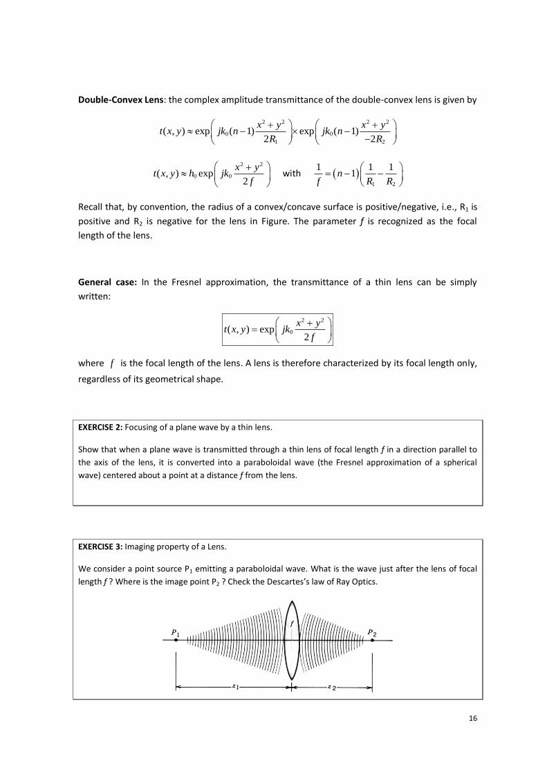
EXERCISE 3: Imaging property of a Lens.
We consider a point source P1 emitting a paraboloidal wave. What is the wave just after the lens of focal
length f ? Where is the image point P2 ? Check the Descartes’s law of Ray Optics.
17
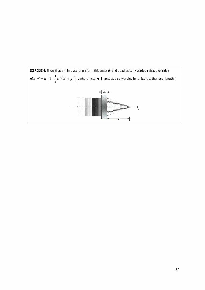
EXERCISE 4: Show that a thin plate of uniform thickness d0 and quadratically graded refractive index
2 2 20
1( , ) 1
2n x y n x y
, where 0 1d , acts as a converging lens. Express the focal length f.

18
Chapter 2: FOURIER OPTICS
1. INTRODUCTION
Fourier optics provides a description of the propagation of light waves based on harmonic
analysis and linear systems.
Harmonic analysis is based on the expansion of an arbitrary function of time as a sum of
harmonic functions of time of different frequencies and different amplitudes:
( ) ( )exp 2
f t f j t d
An arbitrary function ( )f t can be analyzed as a sum of harmonic functions of different
frequencies and complex amplitudes.
The function ( )exp 2 f j t is a harmonic function with frequency and complex amplitude
( )f .
The complex amplitude ( )f , as a function of frequency, is called the Fourier transform of
( )f t :
( ) ( )exp 2
f f t j t dt
This approach is useful for the description of linear systems. If the response of the system to
each harmonic function is known, the response to an arbitrary input function can be determined
(principle of superposition).
The response of a linear system can therefore be determined by the use of harmonic analysis at
the input and superposition at the output.
19
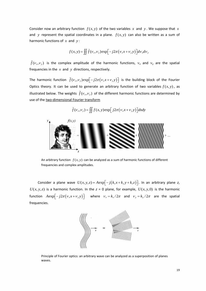
Consider now an arbitrary function ( , )f x y of the two variables x and y . We suppose that x
and y represent the spatial coordinates in a plane. ( , )f x y can also be written as a sum of
harmonic functions of x and y :
( , ) ( , )exp 2x y x y x yf x y f j x y d d
( , )x yf is the complex amplitude of the harmonic functions, x and y are the spatial
frequencies in the x and y directions, respectively.
The harmonic function ( , )exp 2x y x yf j x y is the building block of the Fourier
Optics theory. It can be used to generate an arbitrary function of two variables ( , )f x y , as
illustrated below. The weights ( , )x yf of the different harmonic functions are determined by
use of the two-dimensional Fourier transform
( , ) ( , )exp 2x y x yf f x y j x y dxdy
An arbitrary function ( , )f x y can be analyzed as a sum of harmonic functions of different
frequencies and complex amplitudes.
Consider a plane wave ( , , ) exp x y zU x y z A j k x k y k z . In an arbitrary plane z,
( , , )U x y z is a harmonic function. In the z = 0 plane, for example, ( , ,0)U x y is the harmonic
function exp 2 x yA j x y where / 2x xk and / 2y yk are the spatial
frequencies.
Principle of Fourier optics: an arbitrary wave can be analyzed as a superposition of planes waves.

20
Since an arbitrary function ( , )f x y can be analyzed as a sum of harmonic functions, an
arbitrary optical wave ( , , )U x y z may be analyzed as a sum of plane waves.
If it is known how a linear optical system modifies plane waves, the principle of
superposition can be used to determine the effect of the system on an arbitrary wave.
It is therefore useful to describe the propagation of light through linear optical
components, including free space (free space is a linear system because the wave equation is
linear). The complex amplitudes in two planes normal to the optic (z) axis are regarded as the
input and output of the system.
The transmission of an optical wave ( , , )U x y z through an optical system between an
input plane z = 0 and an output plane z = d. This is regarded as a linear system whose
input and output are the functions ( , ) ( , ,0)f x y U x y and ( , ) ( , , )g x y U x y d ,
respectively.
2. PROPAGATION OF LIGHT IN FREE SPACE
2.1 Correspondence Spatial Harmonic Function / Plane Wave
Consider a plane wave of complex amplitude ( , , ) exp x y zU x y z A j k x k y k z with
wavevector , ,x y zk k kk , wavelength , wavenumber 1 2
2 2 2 2x y zk k k k , and
complex envelope A. The vector k makes angles 1sinx xk k and 1siny yk k with the
y-z and x-z planes, respectively, as illustrated below.
21
The complex amplitude in the z = 0 plane, ( , ,0)U x y , is a spatial harmonic function
( , ) exp 2 x yf x y A j x y with spatial frequencies 2x xk and
2y yk (cycles/mm). The angles of the wavevector are therefore related to the spatial
frequencies of the harmonic function by
1x x and 1y y are the periods of the harmonic function in the x and y
directions. We see that the angles 1sinx x and 1siny y are governed by the
ratios of the wavelength of light to the period of the harmonic function in each direction. The
wavefronts of the wave match to the periodic pattern of the harmonic function in the z = 0
plane.
If kx << k and ky << k, so that the wavevector k is paraxial, the angles x , and y are small and
Thus the angles of inclination of the wavevector are directly proportional to the spatial
frequencies of the corresponding harmonic function.
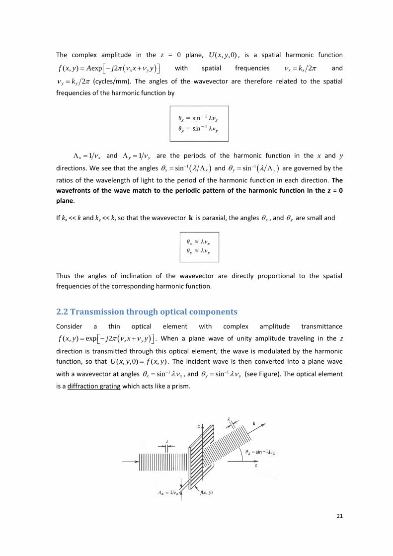
2.2 Transmission through optical components
Consider a thin optical element with complex amplitude transmittance
( , ) exp 2 x yf x y j x y . When a plane wave of unity amplitude traveling in the z
direction is transmitted through this optical element, the wave is modulated by the harmonic
function, so that ( , ,0) ( , )U x y f x y . The incident wave is then converted into a plane wave
with a wavevector at angles 1sinx x , and 1siny y (see Figure). The optical element
is a diffraction grating which acts like a prism.
22
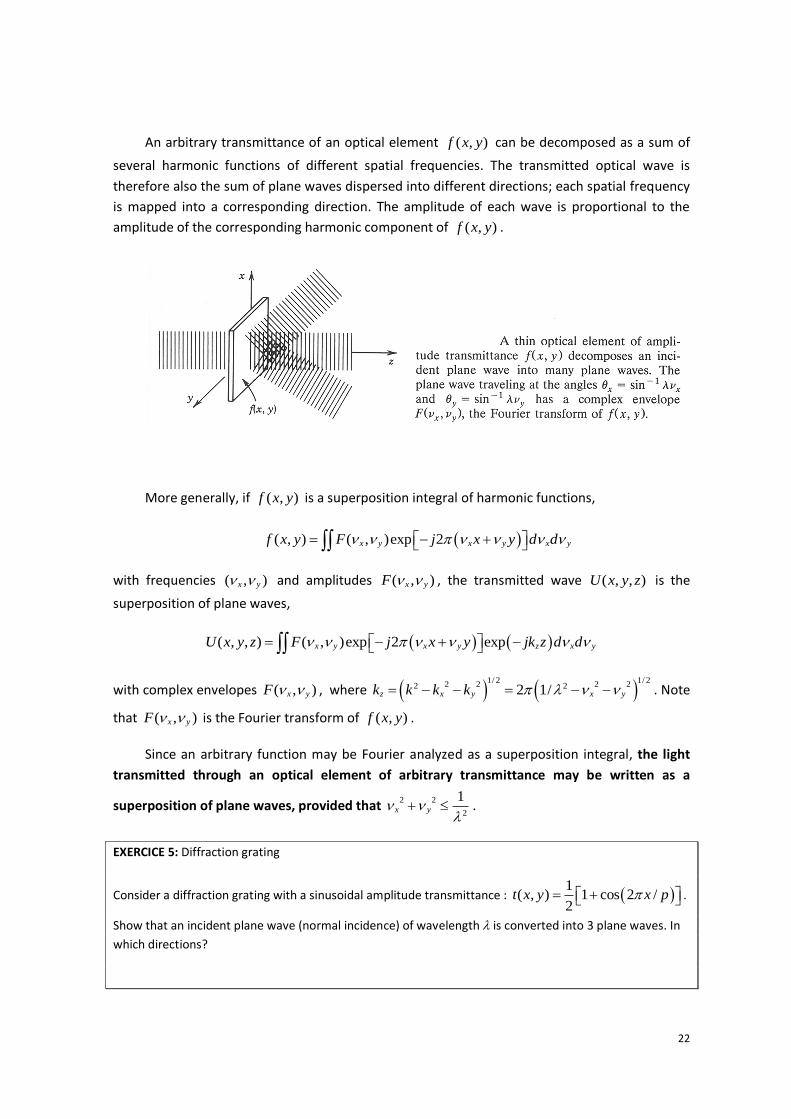
An arbitrary transmittance of an optical element ( , )f x y can be decomposed as a sum of
several harmonic functions of different spatial frequencies. The transmitted optical wave is
therefore also the sum of plane waves dispersed into different directions; each spatial frequency
is mapped into a corresponding direction. The amplitude of each wave is proportional to the
amplitude of the corresponding harmonic component of ( , )f x y .
More generally, if ( , )f x y is a superposition integral of harmonic functions,
( , ) ( , )exp 2x y x y x yf x y F j x y d d
with frequencies ( , )x y and amplitudes ( , )x yF , the transmitted wave ( , , )U x y z is the
superposition of plane waves,
( , , ) ( , )exp 2 expx y x y z x yU x y z F j x y jk z d d
with complex envelopes ( , )x yF , where 1/ 2 1/ 2
2 2 2 22 22 1/z x y x yk k k k . Note
that ( , )x yF is the Fourier transform of ( , )f x y .
Since an arbitrary function may be Fourier analyzed as a superposition integral, the light
transmitted through an optical element of arbitrary transmittance may be written as a
superposition of plane waves, provided that 2 2
2
1x y
.
EXERCICE 5: Diffraction grating
Consider a diffraction grating with a sinusoidal amplitude transmittance : 1
( , ) 1 cos 2 /2
t x y x p .
Show that an incident plane wave (normal incidence) of wavelength is converted into 3 plane waves. In
which directions?

23
2.3 Transfer function of free space
As seen before, the complex amplitude of a plane wave can be written as
( , , ) exp
exp exp
exp 2 exp
x y z
x y z
x y z
U x y z A j k x k y k z
A j k x k y jk z
A j x y jk z
where
2 , 2 .x x y yk k
A plane wave at z d is equal to this plane wave at 0z (harmonic function
exp 2 x yA j x y ) multiplied by the phase factor exp zjk d .
Since 2 2 22
x y zk k k k (Helmholtz)
1/ 2 1/ 2
2 2 2 22 22 1/z x y x yk k k k
If 2 2
2
1x y
,then zk is real. The sign of zk depends on the direction of
propagation. Here we consider a propagation in the direction of increasing z (+ sign).
We can then write
( , , ) ( , ,0) ( , )x yU x y d U x y H
where
1/ 2
2 2
2
1( , ) exp 2x y x yH j d
H is called the transfer function of free space.
The magnitude of the transfer function ( , ) 1x yH . The intensity of a plane wave is not
modified during propagation, but it undergoes a phase change.
If 2 2
2
1x y
,then
1/ 22 2 22 1/z x yk j . The transfert function is now
real: 1/ 2
2 2
2
1( , ) exp 2x y x yH d
. The + sign gives an exponentially
growing function, which is physically unacceptable. We have therefore

24
1/ 2
2 2
2
1( , ) exp 2x y x yH d
, which represents an attenuation factor.
The wave is then called an evanescent wave. We may therefore regard 1/ as the
cutoff frequency of the system. Features contained in spatial frequencies greater than
1/ (details smaller than ) cannot be transmitted by an optical wave over distances
much greater than the wavelength . The spatial resolution of imaging system in the
“far field” is limited by the wavelength. Near-filed optical imaging was demonstrated
recently to achieve super-resolution (not limited by the wavelength).
Fresnel approximation
The expression for the transfer function may be simplified if the spatial frequencies are such that 2 2 21/x y .
1/ 21/ 2
2 2 2 2 2
2
22 2 2 4 2 2
1 11
11 ...
2 8
x y x y
x y x y
We can approximate the transfer function by
2 2( , ) exp expx y x yH jkd j d
In this approximation, the phase is a quadratic function of the spatial frequencies. This
approximation is known as the Fresnel approximation.
The condition of validity of the Fresnel approximation is that
1/ 2
32
2 228
x y d . Noting 2 2 2 2 2 2x y x y , the condition of validity can
be rewritten as :
4
14
d
If a is the largest radial distance in the output plane, the largest angle is /m a d . The condition
of validity of the Fresnel approximation may be written in the form
2
14
F mN
where 2 /FN a d is the Fresnel number.

25
Input-output relation
Given an arbitrary monochromatic wave with complex amplitude ( , , )U x y z at 0z . It can be
decomposed into a sum of plane waves:
( , ,0) ( , ,0)exp 2x y x y x yU x y U j x y d d
( , ,0)x yU is the Fourier transform of ( , ,0)U x y . It represents the complex envelop of plane-
wave components at 0z :
( , ,0) ( , )x yU FT U x y ( , ,0) ( , )exp 2x y x yU U x y j x y dxdy
The complex envelop of plane-wave components at z d is :
( , , ) ( , ,0) ( , )x y x y x yU d U H
The complex amplitude of the wave ( , , )U x y z at z d is the sum of the contribution of
these plane waves :
( , , ) ( , , )exp 2x y x y x yU x y d U d j x y d d
1( ) (0)U d FT FT U H
( , )x yH
( , ,0)U x y
( , ,0)x yU ( , , )x yU d
( ', ', )U x y d
FT FT-1
2 2( , ) exp expx y x yH jkd j d
( , )x yH
( , ,0)U x y
( , ,0)x yU ( , , )x yU d
( ', ', )U x y d
FT FT-1
2 2( , ) exp expx y x yH jkd j d
26
2.4 Impulse-response function of free space
From 1( ) (0)U d FT FT U H , we see that 1( ) (0) ( )U d U FT H (convolution). The
inverse Fourier transform of the Transfer function is called the impulse-response function*:
2 2
0 0( , ) exp exp2
x y jh x y h jk with h jkd
d d
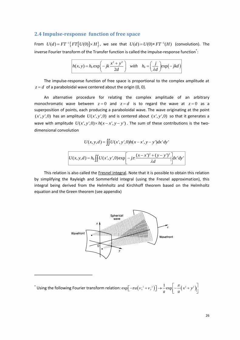
The impulse-response function of free space is proportional to the complex amplitude at
z d of a paraboloidal wave centered about the origin (0, 0).
An alternative procedure for relating the complex amplitude of an arbitrary
monochromatic wave between 0z and z d is to regard the wave at 0z as a
superposition of points, each producing a paraboloidal wave. The wave originating at the point
( ', ',0)x y has an amplitude ( ', ',0)U x y and is centered about ( ', ',0)x y so that it generates a
wave with amplitude ( ', ',0) ( ', ')U x y h x x y y . The sum of these contributions is the two-
dimensional convolution
( , , ) ( ', ',0) ( ', ') ' 'U x y d U x y h x x y y dx dy
2 2
0
( ') ( ')( , , ) ( ', ',0)exp ' '
x x y yU x y d h U x y j dx dy
d
This relation is also called the Fresnel integral. Note that it is possible to obtain this relation
by simplifying the Rayleigh and Sommerfeld integral (using the Fresnel approximation), this
integral being derived from the Helmholtz and Kirchhoff theorem based on the Helmholtz
equation and the Green theorem (see appendix)
* Using the following Fourier transform relation: 2 2 2 21
exp expx ya x ya a
27
This result is consistent with the Huygens-Fresnel principle which states that each point on
a wavefront generates an elementary spherical wave. The envelope of these elementary waves
constitutes a new wavefront. Their superposition constitutes the wave in another plane. In the
Fresnel approximation, a spherical wave centered at (0, 0) is approximated by the paraboloidal
wave :
2 2
( , ) exp2
x yh x y jk
d
2.5 Summary
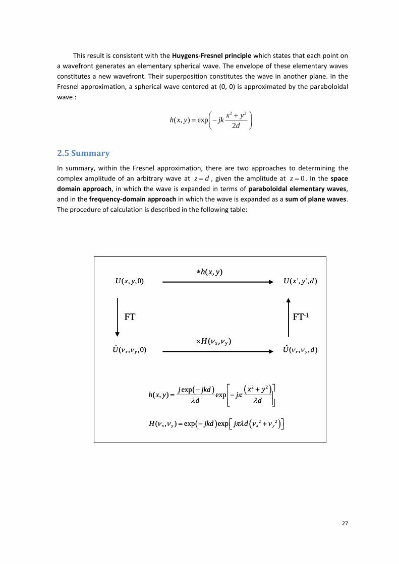
In summary, within the Fresnel approximation, there are two approaches to determining the
complex amplitude of an arbitrary wave at z d , given the amplitude at 0z . In the space
domain approach, in which the wave is expanded in terms of paraboloidal elementary waves,
and in the frequency-domain approach in which the wave is expanded as a sum of plane waves.
The procedure of calculation is described in the following table:
( , )x yH
( , ,0)U x y
( , ,0)x yU ( , , )x yU d
( ', ', )U x y d
FT FT-1
2 2( , ) exp expx y x yH jkd j d
( , )h x y
2 2exp
( , ) expx yj jkd
h x y jd d
( , )x yH
( , ,0)U x y
( , ,0)x yU ( , , )x yU d
( ', ', )U x y d
FT FT-1
2 2( , ) exp expx y x yH jkd j d
( , )h x y
2 2exp
( , ) expx yj jkd
h x y jd d
28
3. OPTICAL FOURIER TRANSFORM
3.1 Amplitude in the far-field
Consider the relation between ( , , )U x y d and ( ', ',0)U x y in the space-domain approach. We
have
2 2
0
( ') ( ')( , , ) ( ', ',0)exp ' '
x x y yU x y d h U x y j dx dy
d
The phase in the exponent is:
2 2 2 2 2 2( / ) ( ') ( ') ( / ) ( ) ( ' ' ) 2( ' ')d x x y y d x y x y xx yy
Suppose that ( ', ',0)U x y is confined to a circle of radius b , and that the distance d is sufficiently
large so that the Fresnel number 2' / 1FN b d .
2 2 2 2( / ) ( ') ( ') ( / )( ) (2 / )( ' ')d x x y y d x y d xx yy
We have then
2 2
0
' '( , , ) exp ( ', ',0)exp 2 ' '
x y xx yyU x y d h j U x y j dx dy
d d
Suppose that ( , , )U x y d is confined to a circle of radius a , and that the distance d is sufficiently
large so that the Fresnel number 2 / 1FN a d . We have then
0
' '( , , ) ( ', ',0)exp 2 ' '
xx yyU x y d h U x y j dx dy
d
We can recognize a Fourier transform:
( , , ) ( , ,0)x y
U x y d Ud d
This approximation is called the Fraunhofer approximation. It is valid when the Fresnel numbers
FN and 'FN are small. The Fraunhofer approximation is more difficult to satisfy than the Fresnel
approximation, which requires that 2 / 4 1F mN . Since 1m in the paraxial approximation, it
is possible to satisfy the Fresnel condition 2 / 4 1F mN for Fresnel numbers FN not necessarily
1.
29
In the Fraunhofer approximation, the complex amplitude ( , , )U x y d of a monochromatic wave
of wavelength , at z d , is proportional to the Fourier transform of the complex amplitude
( , ,0)U x y at 0z , evaluated at the spatial frequencies /x x d and /y y d . The
approximation is valid if ( , ,0)U x y is confined to a circle of radius b satisfying 2 / 1b d and if
( , , )U x y d is confined to a circle of radius a satisfying 2 / 1a d .
EXERCICE 6: Conditions of validity of the Fresnel and Fraunhofer approximations.
Demonstrate that the Fraunhofer approximation is more restrictive than the Fresnel approximation by
taking = 0.5 µm; assuming that the objects points (x, y) lie within a circle of radius a = 1 cm, and
determining the range of distances d for which the two approximations are applicable. The wave is
observed on the axis z.
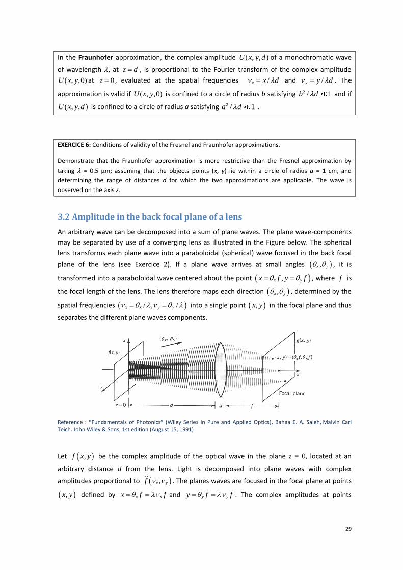
3.2 Amplitude in the back focal plane of a lens
An arbitrary wave can be decomposed into a sum of plane waves. The plane wave-components
may be separated by use of a converging lens as illustrated in the Figure below. The spherical
lens transforms each plane wave into a paraboloidal (spherical) wave focused in the back focal
plane of the lens (see Exercice 2). If a plane wave arrives at small angles ,x y , it is
transformed into a paraboloidal wave centered about the point ,x yx f y f , where f is
the focal length of the lens. The lens therefore maps each direction ,x y , determined by the
spatial frequencies / , /x x y y into a single point ,x y in the focal plane and thus
separates the different plane waves components.
Reference : “Fundamentals of Photonics” (Wiley Series in Pure and Applied Optics). Bahaa E. A. Saleh, Malvin Carl Teich. John Wiley & Sons, 1st edition (August 15, 1991)
Let ,f x y be the complex amplitude of the optical wave in the plane z = 0, located at an
arbitrary distance d from the lens. Light is decomposed into plane waves with complex
amplitudes proportional to ,x yf . The planes waves are focused in the focal plane at points
,x y defined by x xx f f and y yy f f . The complex amplitudes at points

30
,x y in the focal plane are therefore proportional to the Fourier transform of ,f x y
evaluated at /x x f , /y y f .
( , ) ,x y
g x y ff f
To determine the proportionality factor, we analyse the incident wave into its Fourier
components (plane wave decomposition) and propagate them into the optical system. We then
superimpose the contributions of these plane waves in the focal plane. We assume that the
Fresnel approximation is valid.
In the plane 0z ; the plane wave with angles ,x y has a complex amplitude
( , ,0) ( , )exp 2x y x yU x y f j x y . In the plane z d (just before crossing the lens),
the amplitude of the plane wave is ( , , ) ( , )exp 2 ,x y x y d x yU x y d f j x y H ,
with 2 2, exp expd x y x yH jkd j d
.
Upon crossing the lens, the complex amplitude is multiplied by the transmittance of the lens. We
suppose that the lens is very thin ( = 0). Within the Fresnel approximation, the complex
transmittance of the lens is
2 2 2 2
0( , ) exp exp2
x y x yt x y jk j
f f
.
Upon crossing the lens, the amplitude of the plane wave is therefore
( , , ) ( , )exp 2 , ( , )x y x y d x yU x y d f j x y H t x y
By noting
22 2 20 0
22 2 20 0
2 / 2 / ( ) /
2 / 2 / ( ) /
x x
y y
x x f x fx f x x x f
y y f y fy f y y y f
with 0 xx f and 0 yy f ,
the amplitude of the wave can be rewritten
2 2
0 0( , , ) , expx y
x x y yU x y d A j
f
where
2 2, exp exp ( , )x y x y x yA jkd j d f f

31
We recognize here the complex amplitude of a paraboloidal wave (spherical wave) converging
toward the point 0 0,x y in the lens focal plane.
We now have to examine the propagation in free space between the lens and its focal plane. By
using the Fresnel integral, we obtain finally
2
0 0 0( , , ) ,x yU x y d f h f A x x y y
where
0 expj
h jkff
The plane wave is focused into a single point at 0 xx f , 0 yy f .
The last step is to integrate over all the plane waves (all values of x and y ). We finally obtain
0, / , /g x y h A x f y f
or
2 2
2( , ) exp ,l
x y d f x yg x y h j f
f f f
where
2 2exp exp ( , )l x y x yh jkd j d f f
The intensity in the lens focal plane is
2
2
1( , ) ( , )
x yI x y f
f ff
The intensity of light in the back focal plane of the lens is proportional to the squared absolute
value of the Fourier Transform of the amplitude of the wave at the input plane, regardless of the
distance d .
If d f (front focal plane of the lens), we have then
( , ) ,l
x yg x y h f
f f
where
/ exp 2lh j f j kf .

32
The complex amplitude of light at a point ( , )x y in the back focal plane of a lens of focal length f
is proportional to the Fourier transform of the complex amplitude of the complex amplitude in
the front focal plane evaluated at the spatial frequencies /x x f and /y y f . This
relation is valid in the Fresnel approximation. That is why the back focal plane of a lens is called
the Fourier plane. Without lens, the Fourier transformation is obtained only in the Fraunhofer
approximation, which is more restrictive.
4. DIFFRACTION
When an optical wave is transmitted through an aperture and travel some distances in free
space, its intensity is called the diffraction pattern. If light were treated as rays, the diffraction
pattern would be a shadow of the aperture. Because of the wave nature of light, however, the
diffraction pattern may deviate from the aperture shadow, depending on the distance between
the aperture and the observation plane, the wavelength, and dimensions of the aperture.
The aperture is characterized by a transmittance, or aperture function:
1 inside the aperture( , )
0 outside the aperturep x y
The incident wave is multiplied by the aperture function and then propagates in free space.
The diffraction pattern is the intensity distribution of the light at a distance d from the aperture.
The diffraction pattern is known as the Fresnel diffraction or Fraunhofer diffraction, depending
on whether free space propagation is described using the Fresnel approximation or the
Fraunhofer diffraction, respectively.
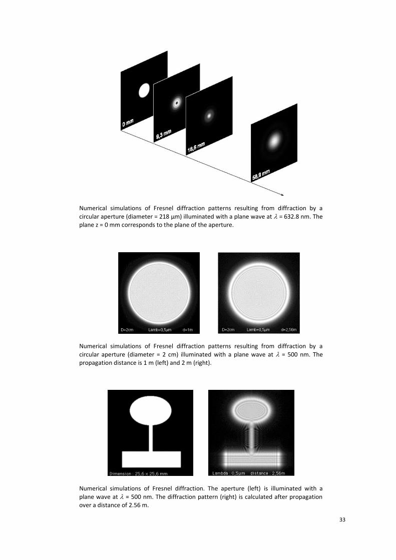
4.1 Fresnel diffraction
The theory of Fresnel diffraction is based on the assumption that the incident wave is multiplied
by the aperture function ( , )p x y and propagates in free space in accordance with the Fresnel
approximation (valid at any distance).
Explicit analytical expression of Fresnel diffraction patterns are often difficult to establish (it
was however easy for a Gaussian wave, see exercise). Numerical simulation are generally
performed (see examples)
33
Numerical simulations of Fresnel diffraction patterns resulting from diffraction by a
circular aperture (diameter = 218 µm) illuminated with a plane wave at = 632.8 nm. The plane z = 0 mm corresponds to the plane of the aperture.
Numerical simulations of Fresnel diffraction patterns resulting from diffraction by a
circular aperture (diameter = 2 cm) illuminated with a plane wave at = 500 nm. The propagation distance is 1 m (left) and 2 m (right).
Numerical simulations of Fresnel diffraction. The aperture (left) is illuminated with a
plane wave at = 500 nm. The diffraction pattern (right) is calculated after propagation over a distance of 2.56 m.
34
Reference : “Fundamentals of Photonics” (Wiley Series in Pure and Applied Optics). Bahaa E. A. Saleh, Malvin Carl Teich. John Wiley & Sons, 1st edition (August 15, 1991)
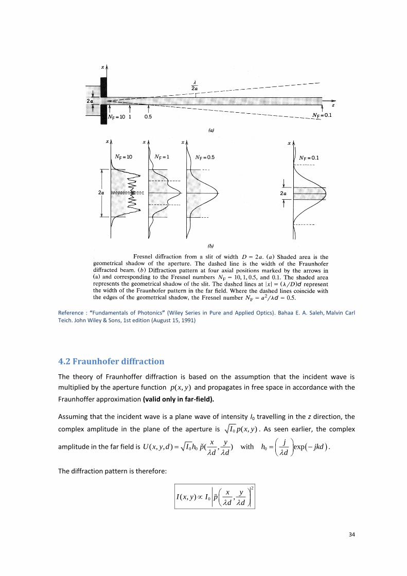
4.2 Fraunhofer diffraction
The theory of Fraunhoffer diffraction is based on the assumption that the incident wave is
multiplied by the aperture function ( , )p x y and propagates in free space in accordance with the
Fraunhoffer approximation (valid only in far-field).
Assuming that the incident wave is a plane wave of intensity I0 travelling in the z direction, the
complex amplitude in the plane of the aperture is 0 ( , )I p x y . As seen earlier, the complex
amplitude in the far field is 0 0 0( , , ) ( , ) with expx y j
U x y d I h p h jkdd d d
.
The diffraction pattern is therefore:
2
0( , ) ,x y
I x y I pd d
35
The Fraunhofer diffraction pattern at the point (x, y) is proportional to the squared magnitude of
the Fourier transform of the aperture function ( , )p x y evaluated at the spatial frequencies
/x x d and /y y d .
The Fraunhofer approximation is valid for distances d that are usually extremely large. They
are satisfied in applications of long-distance free-space optical communication such as laser
radar (lidar) and satellite communication. However, if a lens of focal length f is used to focus the
diffracted light, the intensity pattern in the focal plane is proportional to the squared magnitude
of the Fourier transform of ( , )p x y evaluated at /x x f and /y y f :
2
0( , ) ,x y
I x y I pf f
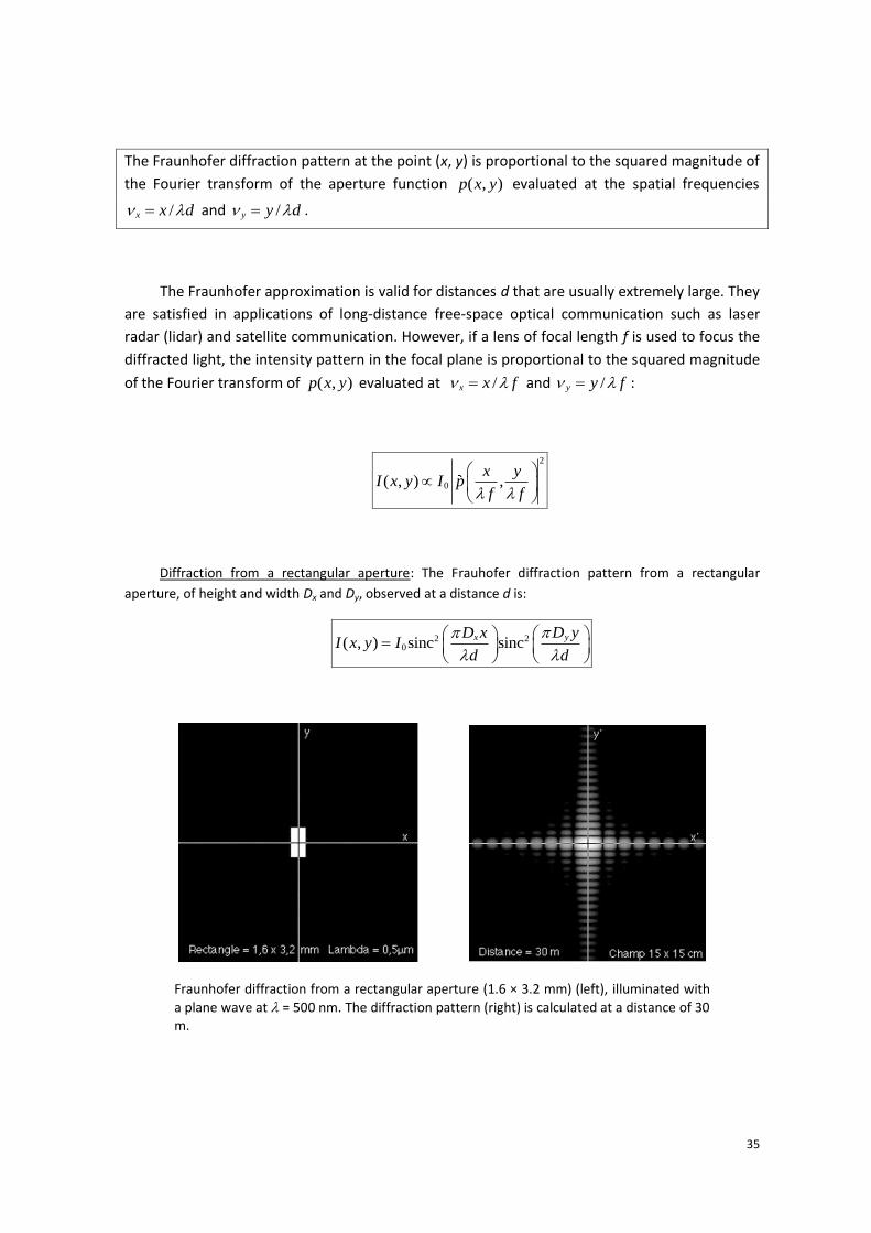
Diffraction from a rectangular aperture: The Frauhofer diffraction pattern from a rectangular
aperture, of height and width Dx and Dy, observed at a distance d is:
2 20( , ) sinc sinc
yx D yD xI x y I
d d
Fraunhofer diffraction from a rectangular aperture (1.6 × 3.2 mm) (left), illuminated with
a plane wave at = 500 nm. The diffraction pattern (right) is calculated at a distance of 30 m.
36
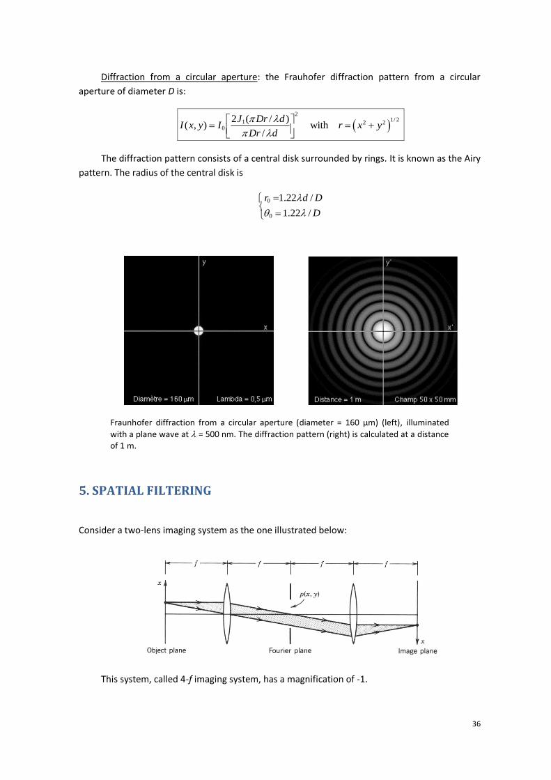
Diffraction from a circular aperture: the Frauhofer diffraction pattern from a circular
aperture of diameter D is:
2
1/ 21 2 20
2 ( / )( , ) with
/
J Dr dI x y I r x y
Dr d
The diffraction pattern consists of a central disk surrounded by rings. It is known as the Airy
pattern. The radius of the central disk is
0
0
1.22 /
1.22 /
r d D
D
Fraunhofer diffraction from a circular aperture (diameter = 160 µm) (left), illuminated
with a plane wave at = 500 nm. The diffraction pattern (right) is calculated at a distance of 1 m.
5. SPATIAL FILTERING
Consider a two-lens imaging system as the one illustrated below:
This system, called 4-f imaging system, has a magnification of -1.
37
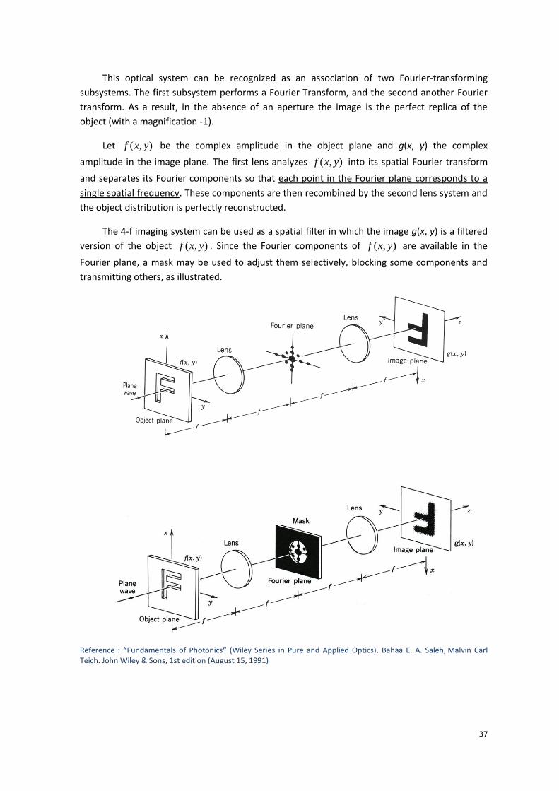
This optical system can be recognized as an association of two Fourier-transforming
subsystems. The first subsystem performs a Fourier Transform, and the second another Fourier
transform. As a result, in the absence of an aperture the image is the perfect replica of the
object (with a magnification -1).
Let ( , )f x y be the complex amplitude in the object plane and g(x, y) the complex
amplitude in the image plane. The first lens analyzes ( , )f x y into its spatial Fourier transform
and separates its Fourier components so that each point in the Fourier plane corresponds to a
single spatial frequency. These components are then recombined by the second lens system and
the object distribution is perfectly reconstructed.
The 4-f imaging system can be used as a spatial filter in which the image g(x, y) is a filtered
version of the object ( , )f x y . Since the Fourier components of ( , )f x y are available in the
Fourier plane, a mask may be used to adjust them selectively, blocking some components and
transmitting others, as illustrated.
Reference : “Fundamentals of Photonics” (Wiley Series in Pure and Applied Optics). Bahaa E. A. Saleh, Malvin Carl Teich. John Wiley & Sons, 1st edition (August 15, 1991)

38
Examples of spatial filters
The ideal low-pass filter has a transmittance represented by the “Disk” function. For example, if
the radius of the disk is r0 and the optical wavelength , the filter eliminates the spatial
frequencies greater than 0 /c r f .
• The high-pass filter is the complement of the low-pass filter. It blocks low frequencies and
transmits high frequencies. The mask is a clear transparency with an opaque central disk. The
filter output is high at regions of large rate of change and small at regions of smooth or slow
variation of the object. This filter is therefore useful for edge enhancement in image-processing
applications.
• The vertical-pass filter blocks horizontal frequencies and transmits vertical frequencies. Only
variations in the x direction are transmitted. If the mask is a vertical slit of width D, the highest
transmitted frequency is ( / 2) /y D f .

39
Composit photo of the moon (a). Filtered photo without horizontal lines (b). Fourier transform (c). Filtered Fourier transform (d).
Reference : “Fundamentals of Photonics” (Wiley Series in Pure and Applied Optics). Bahaa E. A. Saleh, Malvin Carl Teich. John Wiley & Sons, 1st edition (August 15, 1991)
6. Image formation
We consider image formation using the single lens imaging system shown below:
Reference : “Fundamentals of Photonics” (Wiley Series in Pure and Applied Optics). Bahaa E. A. Saleh, Malvin Carl Teich. John Wiley & Sons, 1st edition (August 15, 1991)
40
6.1 Impulse response function
By definition, the impulse response of the complex amplitude in the object plane of the wave
emitted by the point (an impulse) on the optical axis in the object plane. This point emits a
spherical wave, whose complex amplitude in the aperture plane (just before the lens) is
2 2
1
1
( , ) exp2
x yU x y h jk
d
where 1 1
1
expj
h jkdd
Upon crossing the aperture and the lens, the complex amplitude becomes
2 2
1( , ) ( , )exp ,2
x yU x y U x y jk p x y
f
The resultant field 1( , )U x y then propagates in free space a distance d2. The complex amplitude
in the image plane is then obtained by a convolution, according to
2 2
2 1
2
( ') ( ')( , ) ( ', ')exp ' '
x x y yh x y h U x y j dx dy
d
where 2 2
2
expj
h jkdd
We have finally:
2 2
1 2 1
2 2 2
( , ) exp ,x y x y
h x y h h j pd d d
,
where 1p is the Fourier transform of the function 2 2
1( , ) ( , )expx y
p x y p x y j
, and
2 1
1 1 1
d d f .
If the system is focused ( = 0), p1 = p. We have then
2 2
0
2 2 2
( , ) exp ,x y x y
h x y h j pd d d
where 0 1 2h h h .
The function ( , )h x y is called the impulse response function of the imaging system.
If the phase factor 2 2
2
x y
d
is much smaller than 1, it can be neglected, so that
0
2 2
( , ) ,x y
h x y h pd d
The system’s impulse response is proportional to the Fourier transform of the pupil function p.

41
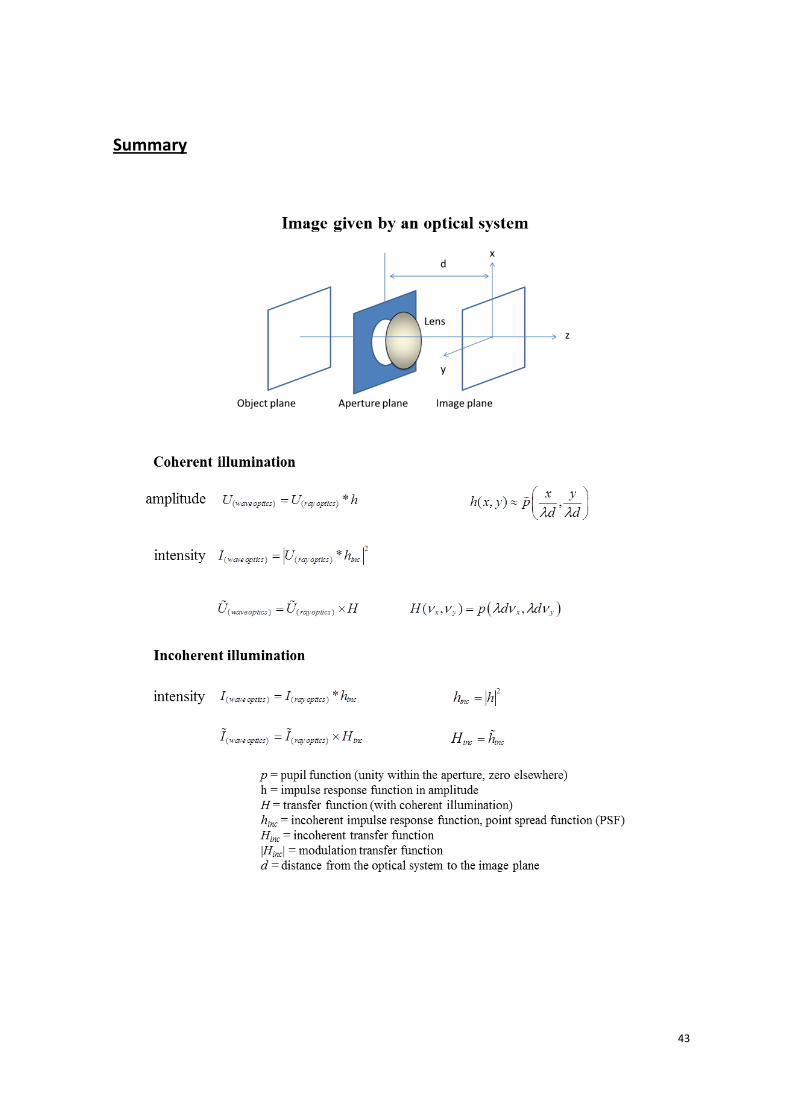
6.2 Image formation with coherent illumination
In the ray optics theory, each point A of the object, located at 0 0,x y , has an image which is a
point A’ located at 0 0', 'x y . In the wave optics theory, the image of the point A is proportional
to the impulse response function centered on A’ : 0 0' ', ' 'h x x y y . The complex amplitude
( )image waveopticsU in the image plane is therefore:
( ) ( ) 0 0 0 0 0 0( ', ') ( ', ') ' ', ' ' ' 'image wave optics image rayopticsU x y U x y h x x y y dx dy
where ( )image rayopticsU is the image obtained by ray tracing. This result can be written in a
condensed manner as using the convolution operator:
( ) ( ) *image waveoptics image rayopticsU U h
The image in amplitude is the perfect image (in amplitude, according to the ray optics theory)
convoluted by the impulse response function.
The spatial frequencies of the wave in the image plane are given by
( ) ( )image waveoptics image rayopticsU U H
where ( , )x yH is the transfert function of the imaging system, defined as the Fourier
transform of the impulse response function.
2 2( , ) ,x y x yH p d d
where ,p x y is the pupil function.
The image in intensity (which is what we can observe on a screen or a camera) is then:
2 2
( ) ( ) *image waveoptics image rayopticsU U h
The description of image formation considered here is valid if we consider coherent light. The concept of coherence will be presented in the next chapter
6.3 Image formation with incoherent illumination
In the previous studies, the light was supposed to be spatially coherent. This means that when
several optical waves are superimposed, the amplitude of the resulting wave is the sum of the
amplitude of each wave. If the light is supposed to be spatially incoherent, this result is not true.
The superposition of several incoherent waves gives a wave whose intensity (and not amplitude)
is the sum of the intensity (and not amplitude) of each wave.
42
The image of a point given by an optical system (the impulse response) has an intensity
2
0 0' ', ' 'h x x y y . The image formation with incoherent illumination is therefore given by
( ) ( ) 0 0 0 0 0 0( ', ') ( ', ') ' ', ' ' ' 'image wave optics image rayoptics incI x y I x y h x x y y dx dy ,
with 2
', ' ', 'inch x y h x y
Using condensed notation, we write :
( ) ( ) *image waveoptics image rayoptics incI I h .
By taking the Fourier transform of the previous relation, we have
( ) ( )image waveoptics image rayoptics incI I H ,
where inc incH h is referred to as the incoherent transfer function of the optical system.
The modulation transfert function is defined as incH .
43
Summary

44
Example: Imaging system with a circular aperture
If the pupil is a circle of radius a, the pupil function , 1p x y for points inside the circle and
zero elsewhere. The pupil function is described by ,r
p x y disa
where 2 2r x y .
The coherent impulse response function of the imaging system is then
1 2
,2
s
s
J rh x y
r
where s
a
d
The incoherent impulse response function is
2
2 1 2, ,
2
s
inc
s
J rh x y h x y
r
(Airy function)
The first zeros of h and inch are located at 1,22s
dr
a
.
With incoherent illumination, each point in the object plane has an image that is proportional to
inch . When two points of the object plane are close enough so that their images are distant of
the quantity sr , then it becomes impossible to resolve them. The quantity 1,22s
dr
a
is a
measure of the resolution of the imaging system.
In the case of coherent illumination, the coherent transfert function of the imaging system is
,x y
s
H dis
where
2 2
x y
In the case of incoherent illumination, the incoherent transfert function of the imaging system is
1/ 22
12cos 1
, if 22 2 2
0 otherwise
inc x y ss s sH
The cutoff frequency is
with coherent illumination
2 with incoherent illumination
c
a
d
a
d
The impulse response functions and tranfert functions with coherent or incoherent illumination
are shown below:

45
Impulse-response functions and transfer functions of a diffraction-limited single lens under coherent (a)
and incoherent (b) illumination. The pupil is supposed to be a circle of radius a.

46
Chapter 3: COHERENCE
In the previous chapters, light was assumed to be deterministic. The dependence of the wave
function on time and position was perfectly predictable. In reality, optical waves have random
fluctuations. For example, light radiated by a hot object (thermal light) is random because it is a
superposition of emissions from a large number of atoms radiating independently and at
different frequencies, amplitudes and phases. Randomness in light may also be a result of
scattering from rough surfaces, diffused glass or turbulent fluids.
The theory of the random fluctuations of light is known as statistical optics or also as the theory
of optical coherence. This theory is based on statistical averaging to define a number of non-
random quantitative measures.
1. Statistical properties of random light
An arbitrary optical wave is defined by a wavefunction ( , ) Re ( , )u t U tr r , where ( , )U tr is the
complex wavefunction. For random light, ( , )U tr is a random function that can be characterized
by a number of statistical averages introduced in this section.
1.1 Optical intensity
The intensity of coherent (deterministic) light is defined as
2( , ) ( , )I t U tr r
47
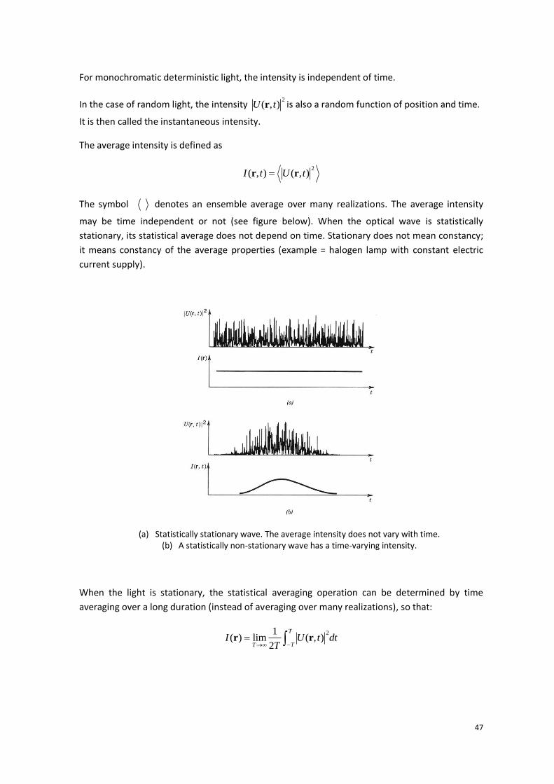
For monochromatic deterministic light, the intensity is independent of time.
In the case of random light, the intensity 2
( , )U tr is also a random function of position and time.
It is then called the instantaneous intensity.
The average intensity is defined as
2( , ) ( , )I t U tr r
The symbol denotes an ensemble average over many realizations. The average intensity
may be time independent or not (see figure below). When the optical wave is statistically
stationary, its statistical average does not depend on time. Stationary does not mean constancy;
it means constancy of the average properties (example = halogen lamp with constant electric
current supply).
(a) Statistically stationary wave. The average intensity does not vary with time. (b) A statistically non-stationary wave has a time-varying intensity.
When the light is stationary, the statistical averaging operation can be determined by time
averaging over a long duration (instead of averaging over many realizations), so that:
21( ) lim ( , )
2
T
TTI U t dt
T r r
48
1.2 Temporal coherence and spectrum
We consider the fluctuation of stationary light as a function of time, at a fixed position. The
random fluctuation of ( )U t can be characterized by a “memory time”. Fluctuations separated by
a time longer than the “memory time” are independent, so that the process “forgets” itself. The
function ( )U t appears to be smooth within the memory time, but “rough” when examined over
a longer time scale. A quantitative measure of this temporal behaviour can be established by
defining a statistical behaviour known as the autocorrelation function.
Temporal coherence function
The autocorrelation function of a stationary complex random function ( )U t is
*( ) ( ) ( )G U t U t
or
*1( ) lim ( ) ( )
2
T
TTG U t U t dt
T
In the theory of optical coherence, the autocorrelation function ( )G is called the temporal
coherence function. This function has a Hermitian symmetry: *( ) ( )G G . The intensity of
the wave is equal to ( )G when 0 : (0)G I . The phase of the function ( )G is equal to
the average of the phase difference between ( )U t and ( )U t . If there is no correlation
between ( )U t and ( )U t , ( ) 0G .
Degree of temporal coherence
The temporal coherence function ( )G carries information about the degree of correlation
(coherence) of stationary light and the intensity. A measure of the coherence that is insensitive
to the intensity is given by the normalized autocorrelation function, known as the degree of
temporal coherence:
*
*
( ) ( )( )( )
(0) ( ) ( )
U t U tGg
G U t U t
(0) 1g . The absolute value of ( )g cannot be greater than one. 0 ( ) 1g
The value of ( )g is a measure of the degree of correlation between ( )U t and ( )U t . In the
case of deterministic and monochromatic light, i.e. 0( ) exp 2U t A j t , ( ) 1g . ( )U t and
( )U t are completely correlated for all time delays .
Usually, ( )g drops from 1 for 0 to 0 for sufficiently large value of .
49
Coherence time / coherence length
The width of ( )g denoted c is a measure of the memory time of the fluctuations known as
the coherence time. For c , the fluctutations are strongly correlated, whereas for c
they are weakly correlated. Although a definition of the width of a function is arbitrary, the usual
definition of the coherence time is the power-equivalent width:
2
( )c g d
The coherence time of monochromatic light is infinite.
The coherence length is defined as
c cl c
Power spectral density
The power spectrale density is defined as 2
( ) ( )S U
The power spectral density is the Fourier Transform of the autocorrelation function. This relation
is known as the Wiener-Khinchin theorem
( ) ( )exp 2S G j d
Demonstration of the Wiener-Khinchin theorem
*( ) ( ) ( )G U t U t dt
( ) ( )exp 2U t U j t d
et * *( ) ( )exp 2U t U j t d
* , , ,
* , , , ,
* , , , ,
*
2
( ) ( )exp 2 ( )exp 2
( ) ( )exp 2 exp 2
( ) ( ) exp 2
( ) ( )exp 2
( )
G U j t d U j t d dt
U U j t j d d dt
U U j d d
U U j d
U
exp 2j d

50
We have ( ) ( )exp 2G S j d
Spectral width
The spectral width of light is defined as the width of the spectral density ( )S . Because of the
Fourier-transform relation between ( )S and ( )G , their widths are inversely related. A light
source of broad spectrum has a short coherence time (and short coherence length).
1c
c c
c
l
Source c cl
Filtered sunlight
(0 = 0.4 – 0.8 µm)
2.67 fs 800 nm
LED (0 = 1 µm, =
50 nm)
67 fs 20 µm
Low-pressure Sodium
lamp
2 ps 600 µm
Multimode He-Ne
laser (0 = 633 nm)
0.67 ns 20 cm
Single-mode He-Ne
laser (0 = 633 nm)
1 µs 300 m
1.3 Spatial coherence
Mutual coherence function
A descriptor of the spatial and temporal fluctuations of the random function ( , )U tr is the cross-
correlation function of 1( , )U tr and 2( , )U tr :
*1 2 1 2( , , ) ( , ) ( , )G U t U t r r r r
This function of the time delay is known as the mutual coherence function. Its normalized
form is called the complex degree of mutual coherence:
1 2
1 2 1 2
1 2
( , , )( , , )
( ) ( )
Gg
I I
r rr r
r r.

51
When the two points coincide ( 1 2 r r r ), ( , , )g r r is the degree of temporal coherence.
The absolute value of the degree of coherence is bounded between zero and unity. It is a
measure of the degree of correlation between the fluctuations at 1r and those at 2r at a time
later.
Degree of spatial coherence
The spatial correlation of light may be assessed by examining the dependence of the mutual
function on position for a fixed time delay ( 0 usually). The mutual coherence function at
0 is
*1 2 1 2( , ,0) ( , ) ( , )G U t U tr r r r
This function is denoted 1 2( , )G r r for simplicity.
Its normalized form called the degree of spatial coherence:
1 2
1 2 1 2
1 2
( , )( , )
( ) ( )
Gg
I I
r rr r
r r
Coherence area
For a given point at 2r , the area scanned by the point 1r within which 1 2( , ) 1/ 2g r r (for
example) is called the coherence area around the point 2r . In the case of perfectly spatially
coherent light the coherence area is infinite. In the case of totally spatially incoherent light the
coherence area is reduced to a point.
It is important to consider the coherence area when using an optical system. If the area of
coherence is greater than the size of the aperture through which light is transmitted, the light
may be regarded as coherent. If the coherence area is smaller than the resolution of the optical
system (size of the system’s incoherent impulse response), the light can be considered as
incoherent.
Light emitted by a hot object (thermal light) with an extended surface has an area of coherence
on the order of 2, where is the central wavelength. It can therefore be considered as spatially
incoherent is most cases. However, complete coherence or incoherence are only idealizations
(two limits of partial coherence).
In a microscope using Köhler illumination, the spatial coherence of illumination can be adjusted
with the aperture diaphragm (D1). The primary advantage of Köhler illumination is to provide
even illumination of the sample.

52
Principle of Köhler illumination in a microscope (in transmission here)
1.4 Gain of spatial coherence by propagation: Zernike and Van Cittert
theorem
We consider a spatially incoherent light source in the plane z = 0. We propose to calculate the
degree of, spatial coherence in an arbitrary plane z after propagation over a distance d.
,,s s and 1 2,r r represent two arbitray points in the plane of the source and in the plane z
respectively. Within the Fresnel approximation, the complex amplitude in the plane z can be
obtained by evaluating the Fresnel integral. We therefore have:
, 2
1* * , 2 ,1
( )( ) exp ( )exp
jU jkd U j d
d d
r sr s s
2
2 22
( )( ) exp ( )exp
jU jkd U j d
d d
r sr s s
The (spatial) mutual coherence function in the plane z is

53
*1 2 1 2
, 2 21 2* , 2 2 ,
2
, 2 21 2* , 2 2 ,
2
( , ) ( ) ( )
1 ( ) ( )( ) ( )exp
1 ( ) ( )( ) ( ) exp
rG U U
U U j d ddd
U U j d ddd
r r r r
r s r ss s s s
r s r ss s s s
Since the light source is supposed to be totally spatially incoherent, the mutual coherence
function in the plane of the source is
* , ,
, ,
( ) ( ) ( , )
( ) ( )
sU U G
I I
s s s s
s s s s, , s s being the Dirac distribution (= 0 for ,s s ).
The mutual coherence function after propagation over a distance d becomes
2 21 2 2
1 2 2
2 2
1 2 2 1 2
2
2 2
1 2 2 1 2
2
1 ( ) ( )( , ) ( )exp
1 ( ).( )exp exp 2
1 ( ).exp ( )exp 2
rG I j ddd
I j j dd dd
j I j dd dd
r s r sr r s s
r r r r ss s
r r r r ss s
2 2
1 2 2 11 2 2
1( , ) exprG j I
d dd
r r r rr r
Its normalized form is
1 22 2
1 21 2( , ) exp
0
Id
g jd I
r r
r rr r
and
1 2
1 2( , )0
Id
gI
r r
r r .
The degree of spatial coherence in the plane z after propagation over a distance d is related to
the Fourier transform of the intensity distribution of the incoherent light source. This result is
known as the Zernike and Van Cittert theorem. Although light is totally spatially incoherence in
the plane of the source, after propagation light is no longer totally incoherent (the light source
having a finite size). In general, light gains spatial coherence by the mere act of propagation. This
result is not surprising. Although light fluctuations at different points in the plan of the source
are uncorrelated, the radiation from each point spreads and overlaps with that from the

54
neighboring points. The light reaching two points in the output plane come from many points in
the source plane, some of which are common. These common contributions create partial
correlation between fluctuations at the output points.
If the area of the source is small, the area of coherence after propagation becomes large. In the
extreme limit of a point source, the area of coherence after propagation is infinite: the wave is
then spatially coherent.
2. Interference of partially coherent light
2.1 Interference and temporal coherence
In a Michelson interferometer (see figure below), a beam splitter generates two identical waves,
one of which having travelled a longer optical path before the two waves are recombined.
A interferometer such as a Michelson interferometer may therefore be used to add a wave to a
replica of a time-delayed replica of itself.
The intensity of light detected at the interferometer output is
2 2 2
I U t U t U t U t U t U t U t U t
We can write
0
0
2 1 Re
2 1 cos
I I g
I g
where g is the degree of temporal coherence of the wave.
The ability of a wave to interfere with a time delayed replica of itself is governed by the degree
of temporal coherence. The visibility of the interference fringes is determined by g .
The function I is called interferogram. It is proportional to the real part of the temporal
autocorrelation of the wave. A Michelson interferometer is thus sometimes called optical
autocorrelator. The width of the interferogram is the coherence length. This quantity can be very
easily measured by using a Michelson-type interferometer. By computing the Fourier transform

55
of the interferogram, the whole spectrum of the light can be obtained. This technique is known
as Fourier-transform spectroscopy.
Since 00
exp 2G I g S j d
(Wiener-Khinchin theorem)
and 00
I S d
we can write
0 02 Re exp 2I S d S j d
or
0
2 1 cos 2I S d
The interferogram can be interpreted as a weighted superposition of interferograms produced
by each of the monochromatic components of the wave. Each component of frequency and
weight S produces an interferogram with period 1/ and unity visibility.
4
Example of interferogram obtained with a halogen lamp of effective spectral width (µm-1); the
horizontal axis is = c .
2.2 Interference and spatial coherence
The effect of spatial coherence on interference can be demonstrated by considering the Young’s
double pinhole interference experiment. A partially coherent wave ,U tr illuminates an
opaque screen with two pinholes located at positions 1r and 2r .

56
Light is diffracted by the two pinholes in the form of spherical waves centered at the pinholes.
The two waves interfere and the intensity I is:
2 2 2 * *1 2 1 2 1 2 1 2I U U U U U U U U
The intensity is observed as a function of x.
We have 1 ,0,0a r , 2 ,0,0ar and ,0,x dr .
Within the Fresnel approximation, the two diffracted spherical wave can be written as
paraboidal waves:
2
1
1 1 1
/ 2, , ,
d x a dU t U t U t
c c
r rr r r
2
2
2 2 2
/ 2, , ,
d x a dU t U t U t
c c
r rr r r
The two waves have equal intensity equal to 0I . The normalized cross-correlation between the
two waves at r is
*1 2
12 1 2
0
( , ) ( , ), , x
U t U tg g
I
r rr r
where
2 2
1 2 2
2x
x a x a axx
c dc dc c
r r r r
is the time delay between the two waves.
If we consider monochromatic light with frequency 0 , 1 2 1 2 0, , , exp 2xg g j r r r r . The
intensity at the interferometer output is then
0 1 2
22 1 , cosI x I g x
r r
57
where 0/c , /x x c and 1 2arg ,g r r . The interference fringe pattern is sinusoidal
with spatial period / and visibility 1 2,g r r .
The visibility of the interference pattern is equal to the magnitude of the degree of spatial
coherence at the two pinholes.