Life Satisfaction and Income in Canadian Urban Neighbourhoods

Research Paper

Life Satisfaction and Income in Canadian Urban Neighbourhoods

by Feng Hou

Social Analysis DivisionOttawa, Ontario

February 2014

Catalogue no. 11F0019M — No. 357ISSN 1205-9153ISBN 978-1-100-23230-0

Analytical Studies Branch Research Paper Series

How to obtain more informationFor information about this product or the wide range of services and data available from Statistics Canada, visit our website, www.statcan.gc.ca.

You can also contact us by

email at [email protected],

telephone, from Monday to Friday, 8:30 a.m. to 4:30 p.m., at the following toll-free numbers:

• Statistical Information Service 1-800-263-1136• National telecommunications device for the hearing impaired 1-800-363-7629• Fax line 1-877-287-4369

Depository Services Program• Inquiries line 1-800-635-7943• Fax line 1-800-565-7757

To access this productThis product, Catalogue no. 11F0019M, is available free in electronic format. To obtain a single issue, visit our website, www.statcan.gc.ca, and browse by “Key resource” > “Publications.”

Standards of service to the publicStatistics Canada is committed to serving its clients in a prompt, reliable and courteous manner. To this end, Statistics Canada has developed standards of service that its employees observe. To obtain a copy of these service standards, please contact Statistics Canada toll-free at 1-800-263-1136. The service standards are also published on www.statcan.gc.ca under “About us” > “The agency” > “Providing services to Canadians.”

Published by authority of the Minister responsible for Statistics Canada

© Minister of Industry, 2014

All rights reserved. Use of this publication is governed by the Statistics Canada Open Licence Agreement (http://www.statcan.gc.ca/reference/licence-eng.htm).

Cette publication est aussi disponible en français.

Standard symbolsThe following symbols are used in Statistics Canada publications:

. not available for any reference period

.. notavailableforaspecificreferenceperiod

... not applicable0 true zero or a value rounded to zero0s value rounded to 0 (zero) where there is a meaningful

distinction between true zero and the value that was rounded

p preliminaryr revisedx suppressedtomeettheconfidentialityrequirementsofthe

Statistics ActE use with cautionF too unreliable to be published* significantlydifferentfromreferencecategory(p<0.05)

Note of appreciationCanada owes the success of its statistical system to a long-standing partnership between Statistics Canada, the citizens of Canada, its businesses, governments and other institutions. Accurate and timely statistical information could not be produced without their continued co-operation and goodwill.

http://www.statcan.gc.ca/

mailto:infostats%40statcan.gc.ca?subject=


http://www.statcan.gc.ca/reference/licence-eng.htm

http://www.statcan.gc.ca/reference/licence-eng.htm

Life Satisfaction and Income in Canadian

Urban Neighbourhoods

by

Feng Hou, Statistics Canada

11F0019M No. 357 ISSN 1205-9153

ISBN 978-1-100-23230-0

February 2014

Analytical Studies Research Paper Series

The Analytical Studies Research Paper Series provides for the circulation, on a pre-publication basis, of research conducted by Analytical Studies Branch staff, visiting fellows, and academic associates. The Analytical Studies Research Paper Series is intended to stimulate discussion on a variety of topics, including labour, business firm dynamics, pensions, agriculture, mortality, language, immigration, and statistical computing and simulation. Readers of the series are encouraged to contact the authors with their comments and suggestions.

Papers in the series are distributed to research institutes and specialty libraries. These papers can be accessed for free at www.statcan.gc.ca.

Publications Review Committee Analytical Studies Branch, Statistics Canada

24th Floor, R.H. Coats Building Ottawa, Ontario K1A 0T6

Acknowledgements The author would like to thank Aneta Bonikowska, Kristyn Frank, Haifang Huang, Grant Schellenberg, and Christopher Schimmele for advice and comments on various issues related to estimation strategies and interpretation of the results. Any errors are the responsibility of the author.


Analytical Studies – Research Paper Series - 4 - Statistics Canada – Catalogue no. 11F0019M, no. 357

Table of contents Abstract ..................................................................................................................................... 5

Executive summary .................................................................................................................. 6

1 Introduction ......................................................................................................................... 7

2 Locality income and subjective well-being ....................................................................... 8

3 Data, measures, and methods ......................................................................................... 11

3.1 Data ............................................................................................................................ 11

3.2 Measures .................................................................................................................... 12

3.3 Methods ...................................................................................................................... 15

4 Results ............................................................................................................................... 17

4.1 The distribution of life satisfaction and income across geographic areas ..................... 17

4.2 The effects of locality income at three geographic levels ............................................. 20

5 Conclusion and discussion ............................................................................................. 29

References .............................................................................................................................. 31


Abstract This study examines possible positive spillovers and negative consumption externalities of the average income in a geographic area (locality income) on individuals' life satisfaction, focusing on two issues. The first is whether the effect of locality income on life satisfaction is sensitive to the scale of geographic units. The second is how the choice of control variables influences the estimated effect of locality income. The analysis of 142,780 survey respondents nested within 31,000 immediate neighbourhoods, 5,000 local communities, and 430 municipalities suggests that the positive spillovers of locality income are stronger in immediate neighbourhoods and local communities than at the municipality level. The positive association between locality income and life satisfaction to a large extent is attributable to the selective geographic concentration of individuals by income, marital status, and home ownership. Although the analysis does not rule out the existence of negative consumption externalities, their effect, if any, does not override the positive spillovers.

Keywords: subjective wellbeing, life satisfaction, relative income, neighbourhood, community.


Executive summary An emerging area of subjective well-being (SWB) research is centered on the differences in the levels of SWB both across countries and among geographic regions within a country. The consideration of geographic differences would extend our knowledge about the determinants of SWB from "internal" factors of personality traits and individuals' socio-demographic characteristics to "external factors" embedded in individuals' environments. An issue with important theoretical and policy implications is whether the income of others in the same geographic area is associated with individuals' SWB. The association could be positive if people benefit from the improved resources, amenities, and social capital in high-income areas. The association could also be negative if people tend to emulate the lifestyles of their more affluent neighbours. Related empirical studies so far have not come to a consensus on this question. The present study attempts to contribute to this issue in two significant ways. First, this study examines whether the effect of the average income in a geographic area (locality income) on SWB is sensitive to the scale of geographic units. With a very large sample of survey respondents nested within three hierarchical levels of geographic areas, this study provides reliable estimates of the association of SWB with average incomes in immediate neighbourhoods (defined as "census dissemination areas"), local communities ("census tracts"), and municipalities ("census subdivisions"). Second, this study examines how the choice of control variables influences the estimated effect of locality income. By considering the effects of individual demographic and socioeconomic characteristics, self-evaluated general health, and area-level attributes in a sequential manner, it is possible to discuss the likely mechanisms through which locality income is related to individuals' SWB. This study draws nationally representative survey data from two sources: (1) the 2008-to-2011 General Social Survey (GSS); and (2) the 2009-to-2011 Canadian Community Health Survey (CCHS). These surveys provide the life satisfaction measure and other individual-level variables. The 2006 Canadian Census of Population 20% sample microdata file is used to derive locality income and other area-level attributes. The area-level data are merged with individual-level data using common geographic identifiers. The study sample contains 142,780 respondents, nested within 31,024 immediate neighbourhoods, 5,002 local communities, and 430 municipalities.

This study finds that the association between life satisfaction and the average income of others living in the same geographic area is sensitive to the scale of geographic areas, to area-level attributes associated with income, and to the inclusion of self-reported health as a control variable. When the fixed effects of higher geographic units (as a proxy for unmeasured area-level attributes) and self-reported health are not controlled for, both neighbourhood and community incomes are positively and significantly associated with life satisfaction even after taking into account geographic differences in individuals' demographic and socio-economic characteristics, while municipality income is negatively and significantly associated with life satisfaction. When geographic fixed effects are controlled for, the positive association of neighbourhood and community incomes with life satisfaction remains, but the negative effect of municipality income disappears. When self-reported health is further controlled for, none of the effects of neighbourhood, community, and municipality incomes are significant.

These results suggest that locality income has no negative net effect on life satisfaction. Its net effect is more likely to be positive because controlling for self-reported health may over-correct the association of locality income with life satisfaction. The results should not be taken to mean that people do not make social comparisons with their neighbours. However, it is clear that, if negative consumption externalities of neighbours' incomes do exist, their effect is certainly not strong enough to offset the spillovers of high-income neighbours.


1 Introduction An emerging area of subjective well-being (SWB) research is centered on the differences in the levels of SWB both across countries and among geographic regions within a country (e.g.: Brereton et al. 2008; Di Tella et al. 2003; Luttmer 2005; Shields et al. 2009). The consideration of geographic differences would extend our knowledge about the determinants of SWB from "internal" factors of personality traits and individuals' socio-demographic characteristics to "external factors" embedded in individuals' environments. This consideration would further help us examine whether the effects of some "internal" factors on SWB are conditioned by external environments (Clark 2003). The research along the geographic dimension would inform whether any policy initiatives to improve the population's SWB should focus solely on the improvement of individuals' socioeconomic circumstances or should also address community and societal factors. An issue with important theoretical and policy implications in SWB research is whether the income of others in the same geographic area is associated with individuals' SWB. The association could be positive if people benefit from the improved resources, amenities, and social capital in high-income areas. The association could also be negative if people tend to emulate the lifestyles of their more affluent neighbours, that is, "keeping up with the Joneses." Related empirical studies so far have not come to a consensus on this question. The present study attempts to contribute to this issue in two significant ways. First, this study examines whether the effect of the average income in a geographic area (locality income) on SWB is sensitive to the scale of geographic units. With a very large sample of survey respondents nested within three hierarchical levels of geographic areas, this study provides reliable estimates of the association of SWB with average incomes in immediate neighbourhoods (defined as "census dissemination areas"), local communities (defined as "census tracts"), and municipalities (defined as "census subdivisions"). Second, this study examines how the choice of control variables influences the estimated effect of locality income. By considering the effects of individual demographic and socioeconomic characteristics, self-evaluated general health, and area-level attributes in a sequential manner, it is possible to discuss the likely mechanisms through which locality income is related to individuals' SWB. The results of this study indicate that the positive spillovers of locality income are stronger in immediate neighbourhoods and local communities than at the municipality level. Furthermore, the positive association between locality income and SWB to a large extent is attributable to the selective geographic concentration of individuals by income, marital status, and home ownership. Although the results do not rule out the existence of negative consumption externalities of locality income, their effect, if any, certainly does not override possible positive spillovers.

The next section, Section 2, briefly reviews previous studies on the relationship between subjective well-being and locality income, and discusses how research questions of this study are situated within the broad literature. This is followed in Section 3 by a discussion of the data and analytical approaches used in the study. Section 4 ("Results") presents descriptive statistics and estimates from multivariate models. The final section, Section 5, summarizes the findings and reconciles the results with those from previous studies.


2 Locality income and subjective well-being While many of the geographic studies of SWB have focused on the impact of external factors related to the natural environment, including air pollution, noise, and climate, and to spatial amenities, such as proximity to facilities and transportation routes (e.g.: Brereton et al. 2008; van Praag and Baarsma 2005; Welsch 2006), some studies have examined the effects of the socioeconomic environment, particularly average income at various geographic levels. At the national level, the observation that major Western countries experienced substantial real-income growth over the last fifty years without a noticeable rise in self-reported happiness levels leads to the well-known "paradox of affluence" (Easterlin 1995). This paradox is commonly explained by the long-established relative-income effect (or, more generally, interdependent preferences in economics and social comparisons in psychology): individuals' SWB is positively associated with their own income but negatively associated with the incomes of others because the increase in the latter raises social norms or aspirations for more costly consumption (Easterlin 2003; Clark et al. 2008). The negative effect of relative income has been regarded as a standard finding in recent psychological and economic studies of happiness (Clark et al. 2008; Layard 2006). The relative-income thesis has far-reaching implications for tax and expenditure policies (Abel 2005). Is there a "localized" paradox of affluence (Morrison 2011)? Does a negative relationship between relative income and SWB also manifest itself at the local or regional level? Investigation into these questions touches on issues central to the relative-income thesis: With whom do people compare themselves? Do people consider their reference group to be based on residential areas, workplaces, and/or social circles? And how wide are people's spheres of comparison? If people do compare themselves with others in their area of residence, one would expect to find a stronger negative effect of relative income as the geographic scale of reference narrows from the national level, to the regional level, and to the local level because close physical proximity facilitates social contact and increases direct exposure to others (Brereton et al. 2008; Fowler and Christakis 2008). However, empirical tests of the relative-income effect at the local or regional level are not straightforward since many confounding factors could bias the estimate. On the one hand, areas with high income, particularly at the regional level, are often associated with some attributes that may reduce the level of SWB, for instance, high density, expensive housing, high cost of living, traffic congestion, and poor air quality. Failure to control these factors may result in overestimating the negative effect of relative income. On the other hand, local affluence may have positive spillovers that at least partially offset any negative effect of relative income. High-income neighbourhoods generally have better amenities (e.g., green space, recreational facilities, and housing conditions), are safer, and exhibit greater social cohesion, all of which likely promote SWB. Moreover, Wilson (1987) argued that, ceteris paribus, the less affluent derive positive externalities from sharing neighbourhoods with more affluent families as a result of richer institutional resources and/or "learning effects."

Empirical studies on the relationship between locality income and SWB remain too sparse to reach a consensus. Using U.S. data, Luttmer (2005) showed that, controlling for an individual's own income, higher average earnings at the regional level are associated with lower levels of self-reported happiness.1 Furthermore, he showed that an increase in regional-level income and a similarly sized decrease in own income have an equivalent negative effect on happiness. He interpreted these results as suggestive evidence that individuals' utility functions depend on both relative and absolute consumption. Using Canadian survey data and controlling for household income and a host of other individual-level variables, Helliwell and Huang (2010)

1. In the Luttmer study, a region is defined as a public use microdata area (PUMA), with an average population of

150,000. PUMAs are used by the U.S. Census Bureau to partition a state into sub-state areas for statistical reporting purpose. A PUMA is generally the aggregate of small counties or the aggregate of census tracts in large metropolitan areas, with at least 100,000 people.


found a negative association between life satisfaction and average income at the local-community level (census tract, with an average of 4,000 population). As Luttmer did, Helliwell and Huang found that the negative effect of community income on life satisfaction is large enough to mostly offset the positive effect of household income. With similar Canadian data, Barrington-Leigh and Helliwell (2008) further showed a negative effect of relative income at the local-community and metropolitan-area levels (with an average population ranging from 120,000 to 3.8 million), but not at the immediate-neighbourhood level (with an average population of 400 to 700 people) or municipality level (with an average population of about 50,000). A New Zealand study suggests that happiness at the sub-national level does not mirror the geographic distribution of wealth, although the result is interpreted as the effect of growth in population size and density (Morrison 2011). Knight et al. (2009) found a negative effect of making intra-village comparisons in rural China—having income above the village average increases the reported happiness level while having income below the village average reduces the happiness level. Other studies have tended to find either no significant effect or a positive effect of locality income. In examining how happiness spreads in social networks with U.S. data, Fowler and Christakis (2008) suggested that the geographic distribution of happiness is not systematically related to local levels of income and education. An Australian study found that the absence of economic deprivation is positively correlated with individual life satisfaction (Shields et al. 2009). A study based on a 1993 South Africa survey found that higher income among other households in a small community (with an average of 2,900 population) increases subjective well-being but that average income in a wider area—the district (with an average population of 125,000)—weakly decreases happiness (Kingdon and Knight 2007). It is difficult to directly resolve the divergent results from previous empirical studies because they differ not only in the geographic scale and the inclusion of various potential confounding factors, but also in broad societal contexts. Within a same country, however, it is possible to test the sensitivity of the relationship between SWB and locality income to the choices of geographic scales and control variables. One purpose of this study is to carefully examine the impact of geographic scale on the relationship between SWB and locality income.2 There are reasons to expect that geographic scale matters. Others' incomes may have both negative consumption externalities and positive spillovers, and the two opposite effects are likely to diminish at different rates as spatial distance increases. It is possible that the decline in the strength of effects with increased distance from the immediate community is steeper for positive spillovers than for consumption externalities, since people can benefit more directly from social ties and improved amenities in their immediate surroundings, while social comparisons with people far away can be sustained through work, other social contact, media, and travel. In short, the positive spillovers of others' incomes may offset negative consumption externalities more so in immediate neighbourhoods than in broad regions. The second purpose of the present study is to examine how the choice of control variables affects the estimated relationship between SWB and locality income. Since survey data normally do not contain direct measures of positive spillovers and negative consumption externalities, only the net effect of others' incomes can be empirically estimated when a reasonable set of potential covariates are taken into account. What are the key control variables to consider? Individual demographics, socio-economic status, and ideally some measures of personality traits are necessarily needed to control for selective sorting of people across areas.

2. Barrington-Leigh and Helliwell (2008) have also addressed this issue. However, their study is based on a much

smaller sample. For instance, only about 9000 respondents in their study are nesting simultaneously in neighbourhoods, local communities, and municipalities, while the sample size in the current study is 15 times larger. More importantly, the present study differs from that of Barrington-Leigh and Helliwell in modelling approaches, particularly in terms of the sequence of entering control variables.


Selective sorting refers to the tendency of people not to randomly choose their place of residence and the possibility that certain factors affecting people's residential choices may also affect their life satisfaction. Area-level attributes are another type of variable that may be correlated with both locality income and SWB but is often not fully taken into account in analyses. The omission of such variables would bias the estimated effect of locality income. This study addresses this issue by including area-level socio-demographic attributes and the fixed effects of higher geographic units as control variables. Such controls, particularly the fixed effects of higher geographic units, would effectively take into account possible negative effects of some environmental factors which may otherwise be confused with negative consumption externalities (Barrington-Leigh and Helliwell 2008). However, such controls, especially at the local level, may take away some of the positive spillovers of others' income, such as recreational facilities, green space, and safety, because these amenities often function beyond one's immediate neighbourhood and extend to the entire local community. Therefore, it is likely that the estimated net effect of others' incomes may weigh more heavily on negative consumption externalities.

Some control variables are more problematic. They are potentially endogenous but routinely included as determinants of SWB in empirical studies. If such variables are also strongly associated with locality income, their inclusion as control variables would bias the likely association between SWB and locality income. An obvious candidate is self-reported health. Self-reported health can be associated with SWB in three ways: as a health effect, as a personality traits effect, and simply as a part of SWB. Better health certainly improves happiness (Blanchflower 2009; Easterlin 2003), but self-reported health may capture more than physical and mental health.3 It may also reflect certain personality traits. People who are more optimistic about their lives are likely to over-report both their SWB and their general health status (Helliwell and Huang 2010; Morrison 2011). More importantly, both SWB and self-reported health are people's self-evaluation of their lives and thus likely represent related features of individuals' global welfare (Borgonovi 2008; Oshio and Kobayashi 2010; Subramanian et al. 2005; Veenhoven 2000). Given that self-reported health is also highly correlated with locality income (Hou and Myles 2005; Macintyre et al. 2002; Stafford and Marmot 2003), the overlap of self-reported health with SWB would pick up a large part of the positive effect of locality income on SWB. This study carefully examines the extent to which self-reported health confounds the estimated effect of locality income on life satisfaction.

3. Happiness also protects health (Diener and Chan 2011; Siahpush et al. 2008; Veenhoven 2008). The reciprocal

relationship between SWB and health cannot be sorted out with cross-sectional survey data.


3 Data, measures, and methods

3.1 Data

This study draws nationally representative survey data from two sources: (1) the 2008-to-2011 General Social Survey (GSS); and (2) the 2009-to-2011 Canadian Community Health Survey (CCHS). These surveys provide the life satisfaction measure and other individual-level variables. The 2006 Canadian Census of Population 20% sample microdata file is used to derive locality income and other area-level attributes. The area-level data are merged with individual-level data using common geographic identifiers.

Statistics Canada's GSS is an annual, nationally representative survey targeting the Canadian population aged 15 and over. Each GSS contains a set of standard socio-demographic questions common across years and a set of unique questions focusing on specific social policy issues. The four GSS data files used here focus on social networks (2008), victimization (2009), time use (2010), and family (2011). The GSS is conducted through computer-assisted telephone interviewing, with response rates ranging from 55% (2010) to 66% (2011). The total sample size is 20,401 for the 2008 survey, 19,422 for the 2009 survey, 15,390 for the 2010 survey, and 22,435 for the 2011 survey.

The CCHS is also a cross-sectional, nationally representative survey. It collects a standard set of demographic and socioeconomic characteristics, as well as a broad range of information on health status, determinants of health, and health system utilization. The CCHS targets the Canadian population aged 12 years and older. About half of the interviews were conducted in person using computer-assisted personal interviewing, and the other half were conducted over the phone using computer-assisted telephone interviewing. The response rate is 73.1% for 2009, 71.5% for 2010, and 69.8% for 2011. The total sample size of CCHS respondents is 61,673 for 2009, 63,197 for 2010, and 63,542 for 2011.

This study pools the data from the two surveys for three reasons. First, these surveys all represent comparable national samples. They have similar sample design and are collected within a relatively short period of four years. Second, these surveys use similar instruments (questions) for life satisfaction and common explanatory variables. As shown in Table 1, the life satisfaction measure and other individual-level control variables in the GSS and CCHS have essentially the same descriptive statistics. Third, and most importantly, pooling similar surveys has the advantage of reducing sampling, coverage, and measurement errors (Schenker and Raghunathan 2007). The combined dataset increases the sample size, and improves the reliability of multi-level regression estimates.4 All analyses are replicated separately with the GSS and CCHS, and no substantive differences are found in main findings, although the estimates tend to have much larger standard errors than those from the pooled sample. Nevertheless, survey type and survey year are controlled for in multivariate models in order to take into account potential differences in patterns of reporting on life satisfaction and other explanatory variables.

This study selects respondents aged 15 and over, residing in Canada's 33 census metropolitan areas (CMAs) and 15 large census agglomerations (CAs) in which census tracts (CTs) are delineated by Statistics Canada.5 The exclusion of respondents in rural areas and small urban 4. In analysis with both individual-level and group-level variables, the estimation of the effects of group-level

variables is equivalent to that from a grouped data model. That is, the group means of the individual-level outcome variables, after adjusting for group differences in individual-level control variables, are regressed on the group-level variables. The reliability of grouped data analysis strongly depends on the average size of observations within each group and the number of groups (Devereux 2007; Raudenbush et al. 2000).

5. A CMA or CA contains one or more adjacent municipalities situated around a major urban core. A CMA must have a total population of at least 100,000, of which 50,000 or more live in the urban core. A CA must have an urban core population of at least 10,000.


areas where CTs are not available is to ensure that the study sample has a complete hierarchical structure so that each respondent has a corresponding neighbourhood, local community, and municipality. Census dissemination areas (DAs) are used as the unit of immediate neighbourhoods. A DA is a small geographic unit composed of one or more adjacent street blocks which has a population of 400 to 700 persons. The DA is chosen as the starting level to analyze the locality income effect because it is within the walking distance of one's home and it is the place where social interactions with neighbours often occur. It is also the smallest standard geographic area for which census data are disseminated and neighbourhood income can be reliably estimated. Above immediate neighbourhoods, CTs are used as the unit of local communities. CTs are compact geographic areas with relatively homogeneous physical characteristics and social living conditions. CT boundaries often follow permanent and easily recognizable physical features. A typical CT consists of about 4,000 individuals. Above local communities, census subdivisions (CSDs) are used as the unit of municipalities—the third-level geographic area in the analysis. A CSD is typically a municipality or a municipal equivalent according to official designations adopted by provincial or federal authorities.

The final sample contains 142,780 respondents (48,880 from the GSS and 93,900 from the CCHS), nested within 31,024 neighbourhoods (with a median area size of 0.2 square kilometre), 5,002 local communities (with a median area size of 1.7 square kilometres), and 430 municipalities (with an average population of 51,600 and a median area size of 110 square kilometres).6 Locality income and other socio-demographic attributes in a geographic area are calculated from the 2006 Census of Population master microdata file. The 2006 Canadian Census of Population drew a 20% random sample of the entire population to collect detailed socioeconomic information on individuals and families. Census variables are estimated on an average sample size of about 100 individuals at the neighbourhood level, 800 individuals at the local-community level, and 10,000 individuals at the municipality level.

3.2 Measures

The outcome variable, life satisfaction, is based on a single question: "How do you feel about your life as a whole right now?" This single-question scale has been used widely by researchers for decades and has been established as a reliable and valid indicator of individuals' subjective well-being (Blanchflower 2009; Diener et al. 2013). There is a slight variation in the life satisfaction scale employed across surveys. In the 2008-to-2010 GSS, a ten-point scale was used in which 1 was associated with "very dissatisfied" and 10 with "very satisfied." In the 2011 GSS and the 2009-to-2011 CCHS, an 11-point scale was used in which 0 was associated with "very dissatisfied" and 10 with "very satisfied." This minor difference in the scale is unlikely to affect the validity of pooling the data from different survey years because, in any given survey/year, less than 2% of respondents reported level 2 or lower, no matter whether the minimum level was 1 or 0 (Bonikowska et al. 2013). Furthermore, the mean life satisfaction level varies much more among survey years using the 10-point scale than between surveys using the 10-point scale and the 11-point scale (see Table 4). Nonetheless, the fixed effects of survey type and year would capture these differences to a large extent.

The individual-level explanatory variables are chosen according to both data availability and their relevance to life satisfaction as revealed in the literature (Blanchflower 2009; Easterlin

6. The distribution of the sample across surveys is the following: 12,581 cases from the 2008 GSS, 12,214 cases

from the 2009 GSS, 9,777 cases from the 2010 GSS, 14,308 cases from the 2011 GSS, 30,609 cases from the 2009 CCHS, 31,573 cases from the 2010 CCHS, and 31,718 cases from the 2011 CCHS. Together, there are about 5 respondents per immediate neighbourhood, 29 respondents per local community, and 332 respondents per municipality.


2003; Helliwell 2003). These variables include age and its squared term, gender, marital status, education, household income, employment status, immigrant status, population group, number of children younger than age 18,7 household size, home ownership, language spoken at home, and self-reported health. The definitions and means (or frequency distributions) of these variables are presented in Table 1. Only a few of these variables need to be discussed further here. Household income is coded as five categories because a large proportion of respondents reported their household income in broad ranges rather than an exact dollar amount and a substantial proportion of respondents did not report their household income (see Table 1). Instead of dropping respondents with missing income from the analysis or imputing income by assuming certain data structure of the missing cases, missing income is treated as a separate category in the household income variable (Hou and Myles 2005; Shields et al. 2009). Since household income categories in the data do not directly take into account the economies of scale associated with family size, household size (its square root) is included as a flexible way to control for the reduced consumption needs of additional family members.8 A separate category is created for missing education, with a treatment similar to that employed for missing income. Self-reported health is based on the question "In general, would you say your health is: excellent, very good, good, fair, or poor?" The variable is coded as 1 (poor) to 5 (excellent).

7. The number of children younger than age 18 is defined differently in the GSS and the CCHS. In the GSS, it is the

number of respondents' single (never married) children 0 to 17 years of age living in the household. In the CCHS, it is the number of persons in the household less than 18 years of age. The mean of the variable is larger in the CCHS (0.62) than in the GSS (0.51).

8. The square root of family size is a conventional scale that discounts the consumption needs of additional family members. Controlling for this factor, the effect of household income on life satisfaction tends to increase. For instance, the coefficients for the lowest and lower middle household income groups (as relative to the higher middle) are -0.47 and -0.19, respectively, without controlling for family size in a model including all other individual-level socio-demographic variables. With the control, they change to -0.50 and -0.21, respectively (as in Model 2, Table 4).


Table 1 Descriptive statistics of individual-level variables

Pooled sample General Social Survey sample

Canadian Community Health

Survey sample

Life satisfaction (points) 7.9 7.9 7.9

Age 44.2 44.1 44.3

Number of children under age 18 0.58 0.51 0.62

Household size (square root) 1.7 1.7 1.6

Self-reported health 3.7 3.6 3.7

Women 51 51 51

Marital status

Married (reference) 50 51 49

Living common-law 10 10 10

Widowed 4 4 4

Divorced or separated 7 7 8

Single 28 28 29

Education

University degree (reference) 27 29 26

Some postsecondary 41 42 41

High school graduate 15 13 16

Less than high school 15 15 14

Level not reported 2 1 3

Immigration status

Canadian-born (reference) 73 74 72

Immigrant 27 26 28

Household income

Lowest: less than $30,000 12 10 14

Lower middle: $30,000 to $59,999 21 19 22

Middle: $60,000 to $99,999 24 22 24

Higher middle: $100,00 to $150,000 (reference) 16 16 16

Highest: more than $150,000 12 12 12

Not reported 15 20 12

Population group

White (reference) 77 79 76

Visible minority 21 18 22

Aboriginal 2 3 2

Employment status

Employed (reference) 64 65 64

Unemployed 5 6 5

Not in labour force 30 29 31

mean

percent

See note at end of table.


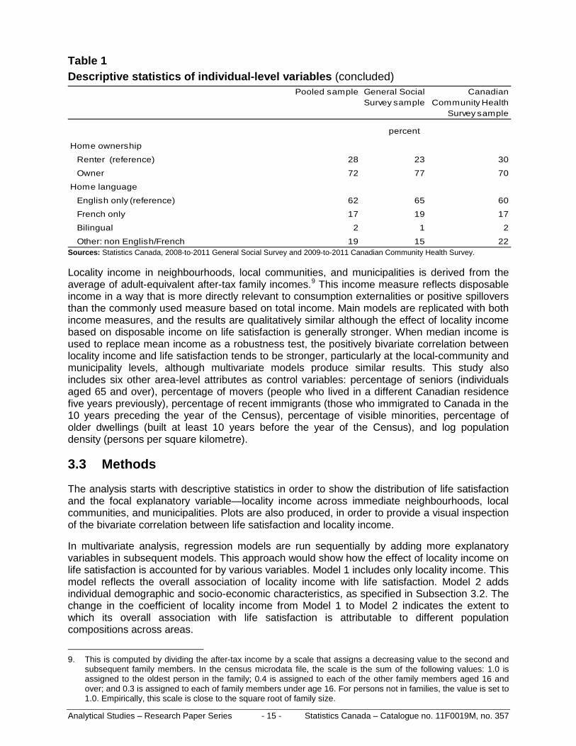
Table 1 Descriptive statistics of individual-level variables (concluded)

Pooled sample General Social Survey sample

Canadian Community Health

Survey sample

percent

Home ownership

Renter (reference) 28 23 30

Owner 72 77 70

Home language

English only (reference) 62 65 60

French only 17 19 17

Bilingual 2 1 2

Other: non English/French 19 15 22Sources: Statistics Canada, 2008-to-2011 General Social Survey and 2009-to-2011 Canadian Community Health Survey.

Locality income in neighbourhoods, local communities, and municipalities is derived from the average of adult-equivalent after-tax family incomes.9 This income measure reflects disposable income in a way that is more directly relevant to consumption externalities or positive spillovers than the commonly used measure based on total income. Main models are replicated with both income measures, and the results are qualitatively similar although the effect of locality income based on disposable income on life satisfaction is generally stronger. When median income is used to replace mean income as a robustness test, the positively bivariate correlation between locality income and life satisfaction tends to be stronger, particularly at the local-community and municipality levels, although multivariate models produce similar results. This study also includes six other area-level attributes as control variables: percentage of seniors (individuals aged 65 and over), percentage of movers (people who lived in a different Canadian residence five years previously), percentage of recent immigrants (those who immigrated to Canada in the 10 years preceding the year of the Census), percentage of visible minorities, percentage of older dwellings (built at least 10 years before the year of the Census), and log population density (persons per square kilometre).

3.3 Methods

The analysis starts with descriptive statistics in order to show the distribution of life satisfaction and the focal explanatory variable—locality income across immediate neighbourhoods, local communities, and municipalities. Plots are also produced, in order to provide a visual inspection of the bivariate correlation between life satisfaction and locality income.

In multivariate analysis, regression models are run sequentially by adding more explanatory variables in subsequent models. This approach would show how the effect of locality income on life satisfaction is accounted for by various variables. Model 1 includes only locality income. This model reflects the overall association of locality income with life satisfaction. Model 2 adds individual demographic and socio-economic characteristics, as specified in Subsection 3.2. The change in the coefficient of locality income from Model 1 to Model 2 indicates the extent to which its overall association with life satisfaction is attributable to different population compositions across areas.

9. This is computed by dividing the after-tax income by a scale that assigns a decreasing value to the second and

subsequent family members. In the census microdata file, the scale is the sum of the following values: 1.0 is assigned to the oldest person in the family; 0.4 is assigned to each of the other family members aged 16 and over; and 0.3 is assigned to each of family members under age 16. For persons not in families, the value is set to 1.0. Empirically, this scale is close to the square root of family size.


Model 3 adds other area-level attributes and the fixed effects of higher-level geographic units to Model 2. The geographic fixed effects control for unmeasured factors that could bias the estimated effect of locality income. For instance, the fixed effects of local communities could, by and large, capture variations across neighbourhoods in recreational facilities and green spaces, which generally benefit residents beyond an immediate neighbourhood. Similarly, the fixed effects of municipalities could capture variations in climate, cost of living, and traffic congestion across local communities. The CMAs/CAs are used as the fixed effects for models with municipality income as the focal explanatory variable. Note that no models include CMA/CA income as the focal explanatory variable owing to the lack of appropriate higher geographic units for the fixed effects.10 The difference in the coefficient of locality income from Model 2 to Model 3 points to the role of area-level attributes and geographic fixed effects in accounting for the association between locality income and life satisfaction. Finally, Model 4 adds self-reported health to Model 3. This variable is added last because it is likely endogenous. Given that self-reported health is strongly correlated with both life satisfaction and locality income, its inclusion may have a strong impact on the coefficient of locality income.

These sequential models are first run separately using immediate-neighbourhood income, local-community income, and municipality income as the focal explanatory variable. This is to make the results of this study comparable to those of previous studies that typically consider the effect of locality income at only one particular geographic level. However, this approach does not clearly address whether the effect of locality income varies with the scale of geographic units, because locality income is highly correlated across hierarchical geographic units. The effect of locality income at a lower geographic level may capture some of the effect of locality income at a higher geographic level. The reverse also applies (Barrington-Leigh and Helliwell 2008). To separate the independent effects of locality incomes at different geographic levels, the above sequential models are repeated but include simultaneously locality incomes measured at immediate neighbourhoods, local communities, and municipalities.

One methodological issue is the treatment of the functional form of life satisfaction. Life satisfaction is an ordinal measure, and the appropriate statistical techniques should be ordered logit models or ordered probit models. However, numerous studies have shown that treating life satisfaction as interval or ordinal makes little difference in the sign and significance of its determinants (Ferrer-i-Carbonell and Frijters 2004; Frey and Stutzer 2000). This is certainly the case with the current data. Only linear model results are presented because it is straightforward to compare changes in the coefficients across these models; this is not the case for logit or probit models (Mood 2010).11 It is also easier to estimate linear models that include a large number of fixed effects (some models contain about 5,000 fixed effects).

Another methodological issue is the multi-level nature of the data. To address this problem, in all regression models, cluster-robust standard errors are estimated in order to take into account correlated errors within an area (Steenbergen and Jones 2002). The level of clustering corresponds to the level of the locality income measures. When locality incomes at the DA, CT, and municipality levels are included in the same model, the DA is used as the level of clustering. Such a model is equivalent to a fixed-intercept model with level-1 covariates within the framework of hierarchical linear models (Raudenbush et al. 2000). This approach essentially

10. The next-higher geographic level is province, which is too broad. For instance, North Bay CMA in northern

Ontario is drastically different from Toronto CMA in southern Ontario in terms of population size, economic scales, population diversity, and climate.

11. This is because log odds ratios or odds ratios from logit or probit regression are affected by unobserved heterogeneity that may be reduced when an additional variable is added to the model even though the added variable is unrelated to the independent variables already in the model.


first estimates the mean outcome for each area, adjusted for differences in individual-level characteristics across areas, and then regresses the mean outcome on area-level predictors.

An additional methodological consideration is the weighting of data from different sources. Both the GSS and the CCHS contain weights to compensate for different sampling rates of different segments of the population. In the regression model with pooled GSS and CCHS data, the weights are standardized so that the sum of the standardized weights equals the sample size within each survey year and type.12

4 Results

4.1 The distribution of life satisfaction and income across geographic areas

The average level of life satisfaction varies strongly across geographic areas, particularly at the immediate-neighbourhood level, as shown in Table 2. To calculate the distribution of average life satisfaction across neighbourhoods (dissemination areas) in Table 2, average life satisfaction is first derived in neighbourhoods with at least 10 respondents. These neighbourhoods are then grouped into quintiles according to their average level of life satisfaction.13 The results show that the average score of life satisfaction among neighbourhoods in the bottom quintile is 1.7 points (out of a maximum 10 points) lower than that among neighbourhoods in the top quintile. The difference in life satisfaction is similarly large between local communities (CTs) in the bottom quintile and those in the top quintile, at 1.4 points. In comparison, among municipalities (CSDs), the difference in life satisfaction is smaller, at 0.7 points, as neighbourhoods with high life satisfaction scores and those with low scores offset each other within a municipality.

Much larger geographic differences exist in income distribution than in life satisfaction. The average family income among neighbourhoods in the top quintile of the income distribution is 2.3 times higher than that among neighbourhoods in the bottom quintile. The corresponding ratio is similarly high at the local-community level, at 2.1 times, but is lower, at 1.6 times, at the municipality level.

12. In the GSS, the average weight ranges from 1500 to 2000 depending on the survey year. In the CCHS, the

average weight is about 640. Standardizing these weights avoids an overestimation of the critical level while maintaining the same distributions as those of non-standardized weights. Alternatively, the weights could be standardized so that the sum of the standardized weights is the same in each survey year and type and equal to the sample size of the smallest survey year and type. Additional analysis (not shown) suggests that there is no substantive difference in model estimates from using either weighting method.

13. Out of the 31,024 immediate neighbourhoods, 3,301 contain at least 10 respondents. Thus, each quintile comprises about 660 neighbourhoods.


Table 2 Distribution of life satisfaction points by quintile across immediate neighbourhoods, local communities, and municipalities

mean standard deviation



Life satisfaction points

First quintile 7.0 0.4 7.2 0.4 7.7 0.1

Second quintile 7.7 0.1 7.7 0.1 7.9 0.0

Third quintile 8.0 0.1 8.0 0.1 8.0 0.0

Fourth quintile 8.3 0.1 8.2 0.1 8.2 0.0

Fifth quintile 8.7 0.2 8.5 0.2 8.5 0.1

Immediate neighbourhoods

Local communities Municipalities

Note: At each geographic level, only the units with at least 10 respondents from the combined General Social Survey and Canadian Community Health Survey files are included in the calculation of means and standard deviations. Sources: Statistics Canada, 2008-to-2011 General Social Survey and 2009-to-2011 Canadian Community Health Survey.

Table 3 Distribution of average adult-equivalent after-tax family income by quintile across immediate neighbourhoods, local communities, and municipalities




Family income (dollars)

First quintile 24,090 3,120 26,090 2,820 30,620 1,030

Second quintile 31,200 1,480 31,740 1,220 34,190 700

Third quintile 35,890 1,410 35,750 1,190 36,710 840

Fourth quintile 41,250 1,830 40,780 1,740 40,240 940

Fifth quintile 54,360 18,500 55,340 15,900 48,080 6,490

Immediate neighbourhoods

Local communities Municipalities

Note: At each geographic level, only the units with at least 10 respondents from the combined General Social Survey and Canadian Community Health Survey files are included in the calculation of means and standard deviations. All numbers are rounded to the nearest 10th. Source: Statistics Canada, 2006 Census of Population 20% microdata file.

The geographic distribution of life satisfaction is correlated with the distribution of income, at least at the immediate-neighbourhood and local-community levels, as shown in Figures 1, 2, and 3. At each geographic level, the average life satisfaction scores in geographic units with at least 10 survey respondents are plotted against these units' log average family income. These plots show a linear relationship between life satisfaction and log average income across neighbourhoods and local communities. At the immediate-neighbourhood level (Figure 1), an increase of one log point is associated with a half-point increase in the life satisfaction score. A similar relation is observed at the local-community level (Figure 2), but not at the municipality level (Figure 3).


Figure 1 Average life satisfaction and family income at the immediate-neighbourhood level

4

5

6

7

8

9

10

9.5 10.0 10.5 11.0 11.5 12.0 12.5log mean family income at the immediate-neighbourhood level

life satisfaction points

Sources: Statistics Canada, 2008-to-2011 General Social Survey, 2009-to-2011 Canadian Community Health Survey, and 2006 Census of Population.

Figure 2 Average life satisfaction and family income at the local-community level

4

5

6

7

8

9

10

9.5 10.0 10.5 11.0 11.5 12.0 12.5log mean family income at the local-community level


Sources: Statistics Canada, 2008-to-2011 General Social Survey, 2009-to-2011 Canadian Community Health Survey, and 2006 Census of Population.


Figure 3 Average life satisfaction and family income at the municipality level

4

5

6

7

8

9

10

9.5 10.0 10.5 11.0 11.5 12.0 12.5log mean family income at the municipality level


Sources: Statistics Canada , 2008-to-2011 General Social Survey, 2009-to-2011 Canadian Community Health Survey, and 2006 Census of Population.

The observed association between life satisfaction and locality income may arise because high-income neighbourhoods and communities have more people with high income and other characteristics positively associated with life satisfaction. If the selective geographic concentration can be controlled for, does life satisfaction still have a significant association with locality income? This is addressed in the following multivariate analyses.

4.2 The effects of locality income at three geographic levels

This subsection first presents in detail the sequential models with immediate-neighbourhood income as the focal explanatory variable. It is followed by a summary of the results from models with the focal explanatory variable being community income and municipality income, respectively, and the results from models with incomes at all three geographic levels.

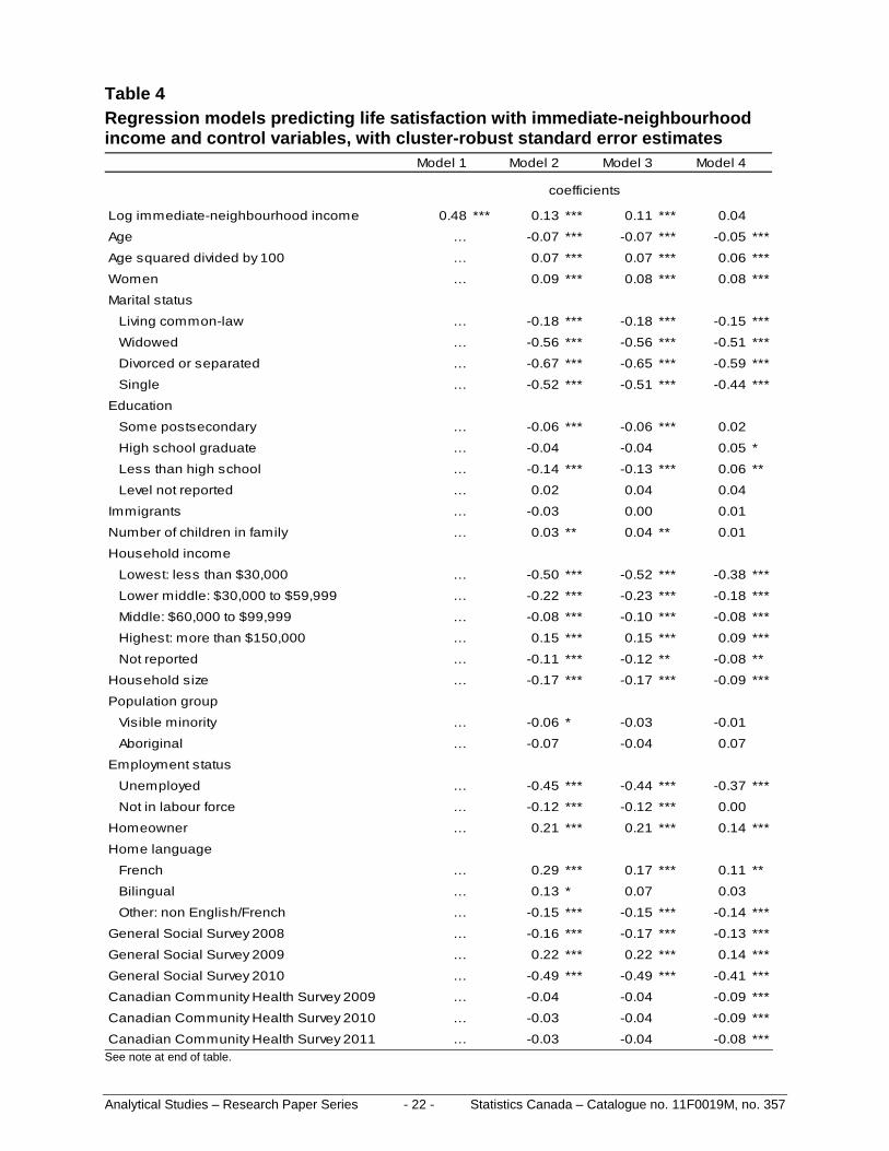
Table 4 presents a series of linear regression models with life satisfaction as the outcome and immediate-neighbourhood income as the focal explanatory variable. Model 1 simply replicates the bivariate association between life satisfaction and immediate-neighbourhood income as illustrated in Figure 1. The coefficient of immediate-neighbourhood income in Model 1 implies that a one-unit increase in immediate-neighbourhood log income is associated with a 0.48-point increase in life satisfaction. This effect is reduced to 0.13 points once individual-level demographic and socioeconomic variables are controlled for in Model 2. The change in the coefficient of immediate-neighbourhood income from Model 1 to Model 2 suggests that over two-thirds (73%) of the observed association between life satisfaction and immediate-neighbourhood income is attributable to selective sorting of people. Further decomposition shows that household income, marital status, and home ownership account for almost all of the change in the coefficient of immediate-neighbourhood income from Model 1 to Model 2.

This decomposition is based on two equations:

( ) ( ) andB - B’ / B = β - β’ / β, (1)


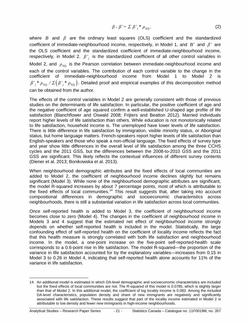
j XZjβ - β’ = Σ β’ * ρ , (2)

where B and β are the ordinary least squares (OLS) coefficient and the standardized coefficient of immediate-neighbourhood income, respectively, in Model 1, and B’ and β’ are the OLS coefficient and the standardized coefficient of immediate-neighbourhood income, respectively, in Model 2. jβ’ is the standardized coefficient of all other control variables in

Model 2, and XZjρ is the Pearson correlation between immediate-neighbourhood income and

each of the control variables. The contribution of each control variable to the change in the coefficient of immediate-neighbourhood income from Model 1 to Model 2 is

( )j XZj j XZjβ’ * ρ / Σ β’ * ρ . Detailed proof and empirical examples of this decomposition method

can be obtained from the author.

The effects of the control variables in Model 2 are generally consistent with those of previous studies on the determinants of life satisfaction. In particular, the positive coefficient of age and the negative coefficient of age squared confirm a well-established U-shaped age profile of life satisfaction (Blanchflower and Oswald 2008; Frijters and Beatton 2012). Married individuals report higher levels of life satisfaction than others. While education is not monotonically related to life satisfaction, household income is. The unemployed have lower levels of life satisfaction. There is little difference in life satisfaction by immigration, visible minority status, or Aboriginal status, but home language matters. French-speakers report higher levels of life satisfaction than English-speakers and those who speak a non-official language. The fixed effects of survey type and year show little differences in the overall level of life satisfaction among the three CCHS cycles and the 2011 GSS, but the differences between the 2008-to-2010 GSS and the 2011 GSS are significant. This likely reflects the contextual influences of different survey contents (Diener et al. 2013; Bonikowska et al. 2013).

When neighbourhood demographic attributes and the fixed effects of local communities are added to Model 2, the coefficient of neighbourhood income declines slightly but remains significant (Model 3). While none of the neighbourhood demographic attributes are significant, the model R-squared increases by about 7 percentage points, most of which is attributable to the fixed effects of local communities.14 This result suggests that, after taking into account compositional differences in demographic and socioeconomic characteristics across neighbourhoods, there is still a substantial variation in life satisfaction across local communities.

Once self-reported health is added to Model 3, the coefficient of neighbourhood income becomes close to zero (Model 4). The changes in the coefficient of neighbourhood income in Models 3 and 4 suggest that the estimated net effect of neighbourhood income strongly depends on whether self-reported health is included in the model. Statistically, the large confounding effect of self-reported health on the coefficient of locality income reflects the fact that this health measure is strongly correlated with both life satisfaction and neighbourhood income. In the model, a one-point increase on the five-point self-reported-health scale corresponds to a 0.6-point rise in life satisfaction. The model R-squared—the proportion of the variance in life satisfaction accounted for by the explanatory variables—increases from 0.15 in Model 3 to 0.26 in Model 4, indicating that self-reported health alone accounts for 11% of the variance in life satisfaction.

14. An additional model is estimated in which DA-level demographic and socioeconomic characteristics are included

but the fixed effects of local communities are not. The R-squared of this model is 0.0785, which is slightly larger than that of Model 2. In this additional model, the coefficient of log locality income is 0.083. Among the included DA-level characteristics, population density and share of new immigrants are negatively and significantly associated with life satisfaction. These results suggest that part of the locality income estimated in Model 2 is attributable to low density and fewer new immigrants in high-income neighbourhoods.


Table 4 Regression models predicting life satisfaction with immediate-neighbourhood income and control variables, with cluster-robust standard error estimates

Model 1 Model 2 Model 3 Model 4

Log immediate-neighbourhood income 0.48 *** 0.13 *** 0.11 *** 0.04

Age … -0.07 *** -0.07 *** -0.05 ***

Age squared divided by 100 … 0.07 *** 0.07 *** 0.06 ***

Women … 0.09 *** 0.08 *** 0.08 ***

Marital status

Living common-law … -0.18 *** -0.18 *** -0.15 ***

Widowed … -0.56 *** -0.56 *** -0.51 ***

Divorced or separated … -0.67 *** -0.65 *** -0.59 ***

Single … -0.52 *** -0.51 *** -0.44 ***

Education

Some postsecondary … -0.06 *** -0.06 *** 0.02

High school graduate … -0.04 -0.04 0.05 *

Less than high school … -0.14 *** -0.13 *** 0.06 **

Level not reported … 0.02 0.04 0.04

Immigrants … -0.03 0.00 0.01

Number of children in family … 0.03 ** 0.04 ** 0.01

Household income

Lowest: less than $30,000 … -0.50 *** -0.52 *** -0.38 ***

Lower middle: $30,000 to $59,999 … -0.22 *** -0.23 *** -0.18 ***

Middle: $60,000 to $99,999 … -0.08 *** -0.10 *** -0.08 ***

Highest: more than $150,000 … 0.15 *** 0.15 *** 0.09 ***

Not reported … -0.11 *** -0.12 ** -0.08 **

Household size … -0.17 *** -0.17 *** -0.09 ***

Population group

Visible minority … -0.06 * -0.03 -0.01

Aboriginal … -0.07 -0.04 0.07

Employment status

Unemployed … -0.45 *** -0.44 *** -0.37 ***

Not in labour force … -0.12 *** -0.12 *** 0.00

Homeowner … 0.21 *** 0.21 *** 0.14 ***

Home language

French … 0.29 *** 0.17 *** 0.11 **

Bilingual … 0.13 * 0.07 0.03

Other: non English/French … -0.15 *** -0.15 *** -0.14 ***

General Social Survey 2008 … -0.16 *** -0.17 *** -0.13 ***

General Social Survey 2009 … 0.22 *** 0.22 *** 0.14 ***

General Social Survey 2010 … -0.49 *** -0.49 *** -0.41 ***

Canadian Community Health Survey 2009 … -0.04 -0.04 -0.09 ***



coefficients



Table 4 Regression models predicting life satisfaction with immediate-neighbourhood income and control variables, with cluster-robust standard error estimates (concluded)


coefficients Immediate neighbourhood

Percentage of seniors … … 0.07 0.06

Percentage of movers … … -0.06 -0.04

Percentage of old dwellings … … -0.04 -0.04

Percentage of recent immigrants … … -0.21 -0.12

Percentage of visible minorities … … 0.17 0.10

Log population density … … 0.00 0.00

Self-reported health … … … 0.60 *** Model 1 Model 2 Model 3 Model 4

Local community fixed effects No No Yes Yes

Model R-squared 0.009 0.078 0.147 0.258 … not applicable *** significantly different from reference category (p<0.001) ** significantly different from reference category (p<0.01) * significantly different from reference category (p<0.05) Note: The sample includes 142,768 respondents nested in 31,017 immediate neighbourhoods (dissemination areas). Sources: Statistics Canada, 2008-to-2011 General Social Survey, 2009-to-2011 Canadian Community Health Survey, and 2006 Census of Population.

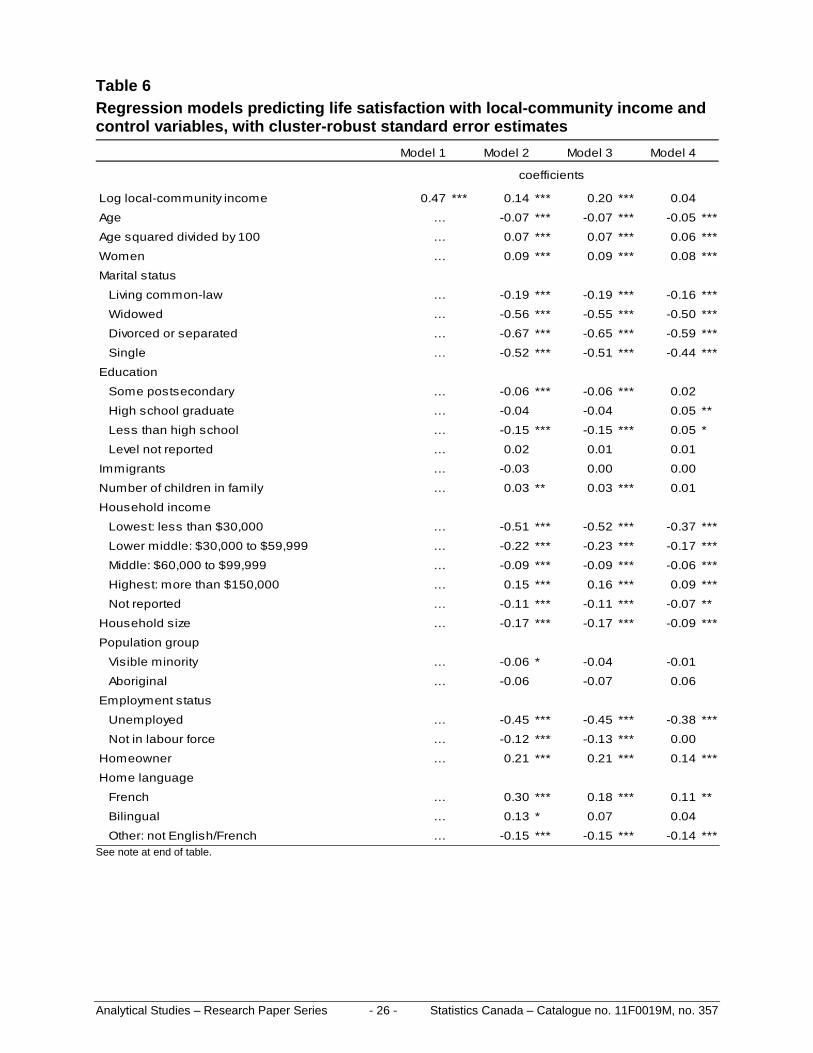
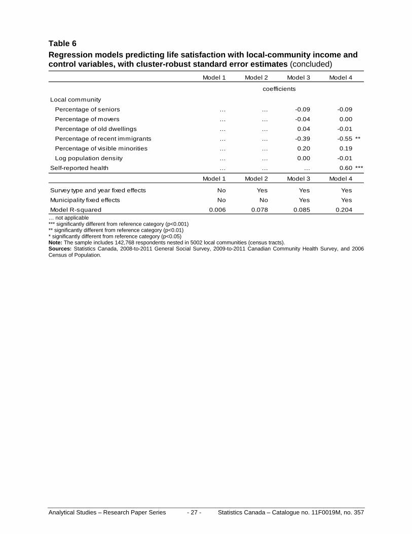
The results of corresponding sequential models with local-community income and municipality income as the focal explanatory variables, as well as models including locality incomes at all three geographic levels, are summarized in Table 5. The detailed model estimates are reported in Tables 6 and 7, which show that the coefficients of individual-level control variables are broadly similar to those in the corresponding models with neighbourhood income as the focal explanatory variable. For easy comparison, Table 5 presents only the coefficient of locality income from those models. The coefficients in the first row are taken from the models with immediate-neighbourhood income as the focal explanatory variable, as in Table 4. The coefficients in the second row are taken from the models with local-community income as the focal explanatory variable, while the coefficients in the third row are taken from the models with municipality income as the focal explanatory variable. The coefficients in the fourth, fifth, and sixth rows are taken from models including simultaneously all three levels of locality income.


Table 5 Comparisons of the regression coefficients of locality incomes in alternative model specifications


Immediate-neighbourhood-level income only

Log immediate-neighbourhood income 0.48 *** 0.13 *** 0.11 *** 0.04

Local-community-level income only

Log local-community income 0.47 *** 0.14 *** 0.20 *** 0.04

Municipality-level income only

Log municipality income 0.05 -0.07 0.17 * -0.04

Three levels nested

Log immediate-neighbourhood income 0.48 *** 0.11 *** 0.10 ** 0.01

Log local-community income 0.15 *** 0.09 ** 0.10 ** 0.03

Log municipality income -0.51 *** -0.23 *** 0.00 -0.04

coefficients


Individual background variables No Yes Yes Yes

Other areal attributes No No Yes Yes

Fixed effects of higher geographic units No No Yes Yes

Self-reported health No No No Yes*** significantly different from reference category (p<0.001) ** significantly different from reference category (p<0.01) * significantly different from reference category (p<0.05) Note: The sample includes 142,768 respondents nested in 31,017 immediate neighbourhoods, 5,002 local communities, and 430 municipalities. Sources: Statistics Canada, 2008-to-2011 General Social Survey, 2009-to-2011 Canadian Community Health Survey, and 2006 Census of Population.

The coefficient of community income is similar in size and significance to that of neighbourhood income in corresponding models (Table 5). These results imply that neighbourhood income and community income are associated with life satisfaction in a similar way. This likely reflects that a local community (defined as a "census tract") is a relatively compact and homogeneous area and that immediate neighbourhoods within a local community are similar in their average incomes.15

In several ways, the results from models with municipality income as the focal explanatory variable differ from models based on neighbourhood or community income (Table 5). There is no overall significant association between life satisfaction and municipality income (third row, Model 1). When individual demographic and socioeconomic characteristics are controlled for, the coefficient of municipality income turns negative, although it is not statistically significant (third row, Model 2). However, when the fixed effects of higher geographic units are taken into account, the coefficient of municipality income becomes significantly positive (Model 3). When self-reported health is further controlled for, the coefficient of municipality income becomes non-significant (Model 4).

As discussed in Subsection 3.3, the effect of locality income estimated separately at each geographic level may partly capture the effect of locality income at a higher or lower geographic

15. In the current data, neighbourhood income is strongly correlated with community income (Pearson r = 0.81).


level. To gauge the independent effects of locality incomes at different geographic levels, nested models that include neighbourhood income, community income, and municipality income simultaneously are estimated.16 The results are presented in the fourth, fifth, and sixth rows of Table 5. The results show that locality incomes at different geographic levels have different associations with life satisfaction. In Model 1, without any other controls, immediate-neighbourhood income has a much larger positive coefficient than local-community income, while municipality income has a large negative coefficient. Once controls for individuals' demographic and socioeconomic characteristics are applied, the positive coefficient of neighbourhood income is reduced much more than is the positive coefficient of community income, and the two become similar in size (Model 2). The large negative coefficient of municipality income also becomes smaller in size.

When the fixed effects of higher geographic areas (CMAs/CAs) are added to Model 2, the coefficients of neighbourhood and community income change only slightly, but the negative coefficient of municipality income becomes not significant (Model 3). When self-reported health is further controlled for, none of the coefficients of neighbourhood, community, and municipality incomes are significant (Table 5, Model 4).

These results suggest that the control of the fixed effects of higher geographic units determines whether the estimated net effect of locality income at the municipality level is significantly negative or non-significant. At this level, high average income is likely associated with attributes that tend to reduce life satisfaction, such as high cost of living, air pollution, and long commuting times. Without controlling for these unmeasured attributes, a significantly negative coefficient of municipality income would be mistakenly interpreted as the effect of consumption externalities. At the neighbourhood and community levels, however, unmeasured locality attributes have little influence on the effect of locality income on life satisfaction. Nevertheless, the inclusion of self-assessed health negates the otherwise positive association between locality income and life satisfaction. This reflects the fact that self-reported health is strongly correlated with neighbourhood and community incomes, but not with municipality income.17

16. In these models, community average income is calculated by excluding a respondent's immediate

neighbourhood, and municipality average income is calculated by excluding a respondent's local community (Barrington-Leigh and Helliwell 2008). The purpose of this procedure is to reduce correlation between locality incomes at various geographic levels. The nested models with three levels of locality income are not affected by multicolinearity. In all models, no coefficient has a variance inflation factor (VIF) value over 2.5. A general rule is that a VIF value of 10 or higher indicates considerable collinearity.

17. In a model similar to Model 3 in Table 5 but one that uses self-reported health as the outcome, the coefficient is 0.16 for neighbourhood income and 0.11 for community income, and both are significant at p<0.001. The coefficient for municipality income is not significant.


Table 6 Regression models predicting life satisfaction with local-community income and control variables, with cluster-robust standard error estimates


Log local-community income 0.47 *** 0.14 *** 0.20 *** 0.04

Age … -0.07 *** -0.07 *** -0.05 ***

Age squared divided by 100 … 0.07 *** 0.07 *** 0.06 ***

Women … 0.09 *** 0.09 *** 0.08 ***

Marital status


Widowed … -0.56 *** -0.55 *** -0.50 ***


Single … -0.52 *** -0.51 *** -0.44 ***

Education


High school graduate … -0.04 -0.04 0.05 **

Less than high school … -0.15 *** -0.15 *** 0.05 *


Immigrants … -0.03 0.00 0.00

Number of children in family … 0.03 ** 0.03 *** 0.01

Household income

Lowest: less than $30,000 … -0.51 *** -0.52 *** -0.37 ***

Lower middle: $30,000 to $59,999 … -0.22 *** -0.23 *** -0.17 ***

Middle: $60,000 to $99,999 … -0.09 *** -0.09 *** -0.06 ***


Not reported … -0.11 *** -0.11 *** -0.07 **

Household size … -0.17 *** -0.17 *** -0.09 ***

Population group


Aboriginal … -0.06 -0.07 0.06

Employment status

Unemployed … -0.45 *** -0.45 *** -0.38 ***


Homeowner … 0.21 *** 0.21 *** 0.14 ***

Home language

French … 0.30 *** 0.18 *** 0.11 **

Bilingual … 0.13 * 0.07 0.04

Other: not English/French … -0.15 *** -0.15 *** -0.14 ***

coefficients



Table 6 Regression models predicting life satisfaction with local-community income and control variables, with cluster-robust standard error estimates (concluded)


coefficients

Local community

Percentage of seniors … … -0.09 -0.09

Percentage of movers … … -0.04 0.00

Percentage of old dwellings … … 0.04 -0.01

Percentage of recent immigrants … … -0.39 -0.55 **

Percentage of visible minorities … … 0.20 0.19

Log population density … … 0.00 -0.01

Self-reported health … … … 0.60 ***


Survey type and year fixed effects No Yes Yes Yes

Municipality fixed effects No No Yes Yes

Model R-squared 0.006 0.078 0.085 0.204… not applicable *** significantly different from reference category (p<0.001) ** significantly different from reference category (p<0.01) * significantly different from reference category (p<0.05) Note: The sample includes 142,768 respondents nested in 5002 local communities (census tracts). Sources: Statistics Canada, 2008-to-2011 General Social Survey, 2009-to-2011 Canadian Community Health Survey, and 2006 Census of Population.


Table 7 Regression models predicting life satisfaction with municipality income and control variables, with cluster-robust standard error estimates


Log municipality income 0.05 -0.07 0.17 * -0.04

Age … -0.07 *** -0.07 *** -0.05 ***

Age squared divided by100 … 0.07 *** 0.07 *** 0.06 ***

Women … 0.09 *** 0.09 *** 0.09 ***

Marital status


Widowed … -0.56 *** -0.56 *** -0.50 ***


Single … -0.52 *** -0.51 *** -0.45 ***

Education


High school graduate … -0.05 * -0.05 * 0.06 **

Less than high school … -0.16 *** -0.16 *** 0.05 *


Immigrants … -0.02 -0.01 0.00

Number of children in family … 0.03 ** 0.03 ** 0.00

Household income

Lowest: less than $30,000 … -0.53 *** -0.54 *** -0.37 ***

Lower middle: $30,000 to $59,999 … -0.23 *** -0.24 *** -0.18 ***

Middle: $60,000 to $99,999 … -0.09 *** -0.09 *** -0.07 ***


Not reported … -0.11 *** -0.11 *** -0.07 **

Household size … -0.17 *** -0.17 *** -0.09 **

Population group


Aboriginal … -0.07 -0.07 0.06

Employment status

Unemployed … -0.45 *** -0.45 *** -0.38 ***


Homeowner … 0.23 *** 0.22 *** 0.15 ***

Home language

French … 0.27 *** 0.18 *** 0.12 ***

Bilingual … 0.11 ** 0.06 0.03

Other: non English/French … -0.16 *** -0.16 *** -0.15 ***

coefficients



Table 7 Regression models predicting life satisfaction with municipality income and control variables, with cluster-robust standard error estimates (concluded)


coefficients

Municipality

Percentage of seniors … … 0.25 0.07

Percentage of movers … … -0.16 -0.02

Percentage of old dwellings … … -0.03 -0.12

Percentage of recent immigrants … … 0.48 0.42 **

Percentage of visible minorities … … -0.11 -0.16

Log population density … … -0.02 * -0.02 *

Self-reported health … … … 0.60 ***


Survey type and year fixed effects No Yes Yes Yes

Metropolitan area fixed effects No No Yes Yes

Model R-squared 0.000 0.078 0.079 0.200 … not applicable *** significantly different from reference category (p<0.001) ** significantly different from reference category (p<0.01) * significantly different from reference category (p<0.05) Note: The sample includes 142,768 respondents nested in 430 municipalities (census subdivisions). Sources: Statistics Canada, 2008-to-2011 General Social Survey, 2009-to-2011 Canadian Community Health Survey, and 2006 Census of Population.

5 Conclusion and discussion Based on a large sample of survey respondents nested within immediate neighbourhoods, local communities, and municipalities, this study finds that the association between life satisfaction and the average income of others living in the same geographic area is sensitive to the scale of geographic areas, to area-level attributes associated with income, and to the inclusion of self-reported health as a control variable. When the fixed effects of higher geographic units (as a proxy for unmeasured area-level attributes) and self-reported health are not controlled for, neighbourhood and community incomes both are positively and significantly associated with life satisfaction even after one takes into account geographic differences in individuals' demographic and socio-economic characteristics, while municipality income is negatively and significantly associated with life satisfaction. When the geographic fixed effects are controlled for, the positive association of neighbourhood and community incomes with life satisfaction remains, but the negative effect of municipality income disappears. When self-reported health is further controlled for, none of the effects of neighbourhood, community, and municipality incomes are significant. How should these results be interpreted?

There is little doubt that observed and unmeasured area-level attributes should be controlled for in estimating the association between locality income and life satisfaction. Some area-level attributes, particularly at the regional level, such as cost of living, population density and diversity, air pollution, and traffic congestion, have little to do with the effect of social comparison or consumption externalities, but they may be positively associated with locality income while negatively associated with life satisfaction. Failure to control for these attributes may lead to the estimated association between locality income and life satisfaction being largely spurious, as clearly illustrated by the large change in the coefficient of municipality income from Model 2 to Model 3 in Table 5. Indeed, the result shown in Model 2 for municipality income as the focal


explanatory variable is similar to the result from Luttmer's main model (2005), where a negative association between locality income and happiness is found. It is possible that the discrepancy between Luttmer's study and the present study originates from the geographic fixed effects in this study.18

It is not straightforward to interpret the confounding effect of self-reported health given the endogenous nature of this variable. If self-reported health captures mainly the mediating effect of health and personality traits, controlling for this variable in estimating the association between life satisfaction and locality income would help to eliminate the impact of individuals' selective geographic concentration. However, if self-reported health is also part of life satisfaction, controlling for self-reported health may take away the part of life satisfaction that is positively associated with locality income. In additional analysis using the 2008 GSS, an objective measure of health (the number of chronic physical and mental illnesses diagnosed by health professionals) and a direct measure of personality traits (mastery) are used to replace self-reported health.19 These two variables jointly take away less than one-third of the positive association of community income with life satisfaction. In comparison, self-reported health alone takes away all positive association of community income with life satisfaction. When chronic illnesses and mastery are entered together with self-reported health, the coefficient of self-reported health on life satisfaction reduces only from 0.58 to 0.46.20 These results seem to suggest that self-reported health represents more than health and personality traits and that the inclusion of self-reported health in the model over-corrects the association of locality income with life satisfaction. The two previous Canadian studies that found a negative effect of community income are based on models controlling for self-reported health as well as a measure of trust in neighbours (Barrington-Leigh and Helliwell 2008; Helliwell and Huang 2010). The latter measure is an indicator of social capital and likely captures some of the positive spillovers of community income. The inclusion of such variables as controls would further move the estimated net effect of locality income towards negative. Thus, the evidence of negative consumption externalities in their studies was found only after exhausting possible positive spillovers.

Overall, the results of this study suggest that locality income has no negative net effect on life satisfaction. Its net effect is more likely to be positive because controlling for self-reported health may over-correct the association of locality income with life satisfaction. The results should not be taken to mean that people do not make social comparisons with their neighbours. However, it is clear that, if negative consumption externalities of neighbours' incomes do exist, the effect is certainly not strong enough to offset the spillovers of high-income neighbours.

18. Luttmer did control for the size of metropolitan area population and fraction of blacks in PUMA. He also

performed an additional test to control for PUMA housing price. These controls, however, may not fully capture other PUMA attributes that may be negatively associated with happiness. The negative coefficient of municipality income in Model 2 in the present study hardly changes when controlling only for other area-level attributes; it changes to positive and significant only when the fixed effects of CMAs/CAs are controlled for.

19. While the causal direction between self-reported health and life satisfaction is in doubt, it is reasonable to assume that chronic physical and mental illnesses can affect individuals' evaluation of their current SWB. Veenhoven (2008) suggests that happiness protects one against falling ill but that it does not cure diseases. Chronic physical and mental illnesses include asthma, arthritis, back problems, high blood pressure, migraine, chronic bronchitis, diabetes, heart disease, cancer, stomach or intestinal ulcers, effects of a stroke, urinary incontinence, bowel disorders, Alzheimer's disease or other dementia, mood disorders (such as depression, bipolar disorder, mania, or dysthymia), and anxiety disorders (such as a phobia, obsessive-compulsive disorder, or panic disorder). The mastery scale measures the extent to which people believe that their life-chances are under their control.

20. Model results are available on request. The 2008 GSS contains only 12,580 respondents nested within 9,538 neighbourhoods, 4,119 communities, and 378 municipalities. Likely as a result of the small sample size and the corresponding larger coverage errors and measurement errors, none of the coefficients of community income in Models 1, 2, 3, and 4 are statistically significant, although the size of the coefficients is similar to that reported in Table 5.


References Abel, A. 2005. "Optimal taxation when consumers have endogenous benchmark levels of consumption." The Review of Economic Studies 72 (1): 21–42. Barrington-Leigh, C., and J. Helliwell. 2008. "Empathy and emulation: Life satisfaction and the urban geography of comparison groups." NBER Working Paper Series, no. 14593. Cambridge, Massachusetts: National Bureau of Economic Research.

Blanchflower, D.G. 2009. "International evidence on well-being." In National Time Accounting and Subjective Well-being, ed. A.B. Krueger, chapter 7, p. 155–226. Chicago: National Bureau of Economic Research and University of Chicago Press.

Blanchflower, D.G., and A.J. Oswald. 2008. "Is well-being U-shaped over the life cycle?" Social Science & Medicine 66: 1733–1749.

Bonikowska, A., J. Helliwell, F. Hou, and G. Schellenberg. 2013. An Assessment of Life Satisfaction Responses on Recent Statistics Canada Surveys. Analytical Studies Branch Research Paper Series, no. 351. Statistics Canada Catalogue no. 11F0019M. Ottawa: Statistics Canada.

Borgonovi, F. 2008. "Doing well by doing good. The relationship between formal volunteering and self-reported health and happiness." Social Science & Medicine 66: 2321–2334.

Brereton, F., P. Clinch, and S. Ferreira. 2008. "Happiness, geography and the environment." Ecological Economics 65: 386–396.

Clark, A. 2003. "Unemployment as a social norm: Psychological evidence from panel data." Journal of Labor Economics 21 (2): 323–351.

Clark, A., P. Frijters, and M.A. Shields. 2008. "Relative income, happiness, and utility: An explanation for the Easterlin Paradox and other puzzles." Journal of Economic Literature 46 (1): 95–144. Devereux, P.J. 2007. "Small-sample bias in synthetic cohort models of labor supply." Journal of Applied Econometrics 22: 839–848.

Diener, E., and M. Chan. 2011. "Happy people live longer: Subjective well-being contributes to health and longevity." Applied Psychology: Health and Well-being 3 (1): 1–43.

Diener, E., R. Inglehart, and L. Tay. 2013. "Theory and validity of life satisfaction scales." Social Indicator Research 112: 497–527. Di Tella, R., R. MacCulloch, and A. Oswald. 2003. "The Macroeconomics of Happiness." The Review of Economics and Statistics 85 (4): 809–827. Easterlin, R. 1995. "Will raising the incomes of all increase the happiness of all?" Journal of Economic Behavior and Organization 27: 35–47.

Easterlin, R. 2003. "Explaining happiness." Proceedings of the National Academy of Sciences 100 (19): 11176–11183. Ferrer-i-Carbonell, A., and P. Frijters. 2004. "How important is methodology for the estimates of the determinants of happiness?" The Economic Journal 114: 641–659.


Frey, B., and A. Stutzer. 2000. "Happiness, economy and institutions." Economic Journal 110: 918–938.

Frijters, P., and T. Beatton. 2012. "The mystery of the U-shaped relationship between happiness and age." Journal of Economic Behavior & Organization 82: 525–542.

Fowler, J.H., and N.A. Christakis. 2008. "Dynamic spread of happiness in a large social network: Longitudinal analysis over 20 years in the Framingham Heart Study." BMJ 337 (768): a2338. Available at: http://www.bmj.com/content/337/bmj.a2338.pdf%2Bhtml (accessed July 23, 2013).

Helliwell, J.F. 2003. "How's Life? Combining Individual and National Variables to Explain Subjective Well-Being." Economic Modelling 20 (2): 331–360.

Helliwell, J.F., and H. Huang. 2010. "How's the Job? Well-Being and Social Capital in the Workplace." Industrial and Labor Relations Review 63 (2): 205–227.

Hou, F., and J. Myles. 2005. "Neighbourhood inequality, neighbourhood affluence and population health." Social Science & Medicine 60: 1557–1569.

Kingdon, G.G., and J. Knight. 2007. "Community, comparisons and subjective well-being in a divided society." Journal of Economic Behavior & Organization 64 (1): 69–90.

Knight, J., L. Song, and R. Gunatilaka. 2009. "Subjective well-being and its determinants in rural China." China Economic Review 20: 635–649.

Layard, R. 2006. "Happiness and public policy: a challenge to the profession." The Economic Journal 116: C24–C33.

Luttmer, E. 2005. "Neighbors as negatives: relative earnings and well-being." The Quarterly Journal of Economics 120: 963–1002.

Macintyre, S., A. Ellaway, and S. Cummins. 2002. "Place effects on health: how can we conceptualise, operationalise, and measure them?" Social Science & Medicine 55: 125–139.

Mood, C. 2010. "Logistic regression: Why we cannot do what we think we can do, and what we can do about it." European Sociological Review 26 (1): 67–82.

Morrison, P. 2011. "Local expressions of subjective well-being: The New Zealand experience." Regional Studies 45 (8): 1039–1058.

Oshio, T., and M. Kobayashi. 2010. "Income inequality, perceived happiness, and self-rated health: Evidence from nationwide surveys in Japan." Social Science & Medicine 70: 1358–1366.

Raudenbush, S.W., A.S. Bryk, Y.F. Cheong, and R.T. Congdon. 2000. HLM 5 Hierarchical Linear and Nonlinear Modeling. Skokie, Illinois: Scientific Software International.

Schenker, N., and T. Raghunathan. 2007. "Combining Information from Multiple Surveys to Enhance Estimation of Measures of Health." Statistics in Medicine 26: 1802–1811.

Shields, M., S. Wheatley Price, and M. Wooden. 2009. "Life satisfaction and the economic and social characteristics of neighbourhoods." Journal of Population Economics 22: 421–443.

Siahpush, M., M. Spittal, and G.K. Singh. 2008. "Happiness and Life Satisfaction Prospectively Predict Self-Rated Health, Physical Health, and the Presence of Limiting, Long-Term Health Conditions." American Journal of Health Promotion 23 (1): 18–26.

http://www.bmj.com/content/337/bmj.a2338.pdf%2Bhtml


Stafford, M., and M. Marmot, 2003. "Neighborhood deprivation and health: does it affect us all equally?" International Journal of Epidemiology 32: 357–366.

Steenbergen, M., and B. Jones. 2002. "Modeling multilevel data structure." American Journal of Political Science 46: 218–237.

Subramanian, S.V., D. Kim, and I. Kawachi. 2005. "Covariation in the socioeconomic determinants of self rated health and happiness: a multivariate multilevel analysis of individuals and communities in the USA." Journal of Epidemiology and Community Health 59: 664–669.

van Praag, B.M.S., and B.E Baarsma. 2005. "Using Happiness Surveys to Value Intangibles: The Case of Airport Noise." Economic Journal 115: 224–246.

Veenhoven, R. 2000. "The four qualities of life." Journal of Happiness Studies 1: 1–39. Veenhoven, R. 2008. "Healthy happiness: effects of happiness on physical health and the consequences for preventive health care." Journal of Happiness Studies 9: 449–469.

Welsch, H. 2006. "Environment and happiness: valuation of air pollution using life satisfaction data." Ecological Economics 58: 801–813.

Wilson, J. 1987. The truly disadvantaged: The inner city, the underclass, and public policy. Chicago: University of Chicago Press.

Life Satisfaction and Income in Canadian Urban Neighbourhoods

Documents

Transcript of Life Satisfaction and Income in Canadian Urban Neighbourhoods