Journal of Economic Growth Volume 4, Issue 3, September 1999, pp. 239-275

Life During Growth

William Easterly1

World Bank

Abstract: A remarkable diversity of indicators shows quality of life across nations to be positively associated with per capita income. At the same time, the changes in quality of life as income grows are surprisingly uneven. Either in levels or changes, moreover, the effect of exogenous shifts over time is surprisingly strong compared to growth effects. This paper reaches this conclusion with a panel dataset of 81 indicators covering up to 4 time periods (1960, 1970, 1980, and 1990). The indicators cover 7 subjects: (1) individual rights and democracy, (2) political instability and war, (3) education, (4) health, (5) transport and communications, (6) inequality across class and gender, and (7) “bads.” With a SUR estimator in levels, income per capita has an impact on the quality of life that is significant, positive, and more important than exogenous shifts for 32 out of 81 indicators. With a fixed effects estimator, growth has an impact on the quality of life that is significant, positive, and more important than exogenous shifts for 10 out of 81 indicators. With a first-differences IV estimator, growth has a causal impact on the quality of life that is significant, positive, and more important than exogenous shifts for 6 out of 69 quality of life indicators. The conclusion speculates about such explanations for the pattern of results as: (1) the long and variable lags that may come between growth and changes in the quality of life, and (2) the possibility that global socioeconomic progress is more important than home country growth for many quality of life indicators.

1 I acknowledge assistance on data collection and organization from a fortuitous succession of two hard-working research assistants, Peter Niessen and Giuseppe Iarossi. An unpublished literature survey by Peter Niessen was helpful as well. I have benefitted from comments of participants at the Poverty-Environment-Growth Workshop at the World Bank including discussants Andrew Steer and Tom Tietenburg and from participants in seminars at the World Bank, George Washington, Harvard, MIT, NYU, Syracuse, the University of Virginia, and the NBER small-group meeting on Growth. Comments from and/or discussions with two anonymous referees, Joshua Aizenman, Ken Chomitz, Richard Easterlin, Raquel Fernandez, Jan Gunning, Dean Jamison, Ross Levine, Norman Loayza, Aart Kraay, Paul Krugman, Martin Ravallion, Jakob Svennson, and Jaume Ventura were extremely helpful. I am most grateful of all to Lant Pritchett, who contributed several rounds of trenchant criticisms. None of these generous commentators should be held responsible for any errors. The views expressed here are those of the author and not of the World Bank or its member governments. The data and full text for this paper are available on the web page http://www.worldbank.org/html/prdmg/grthweb/growth_t.htm

2

I. Introduction Does life during growth get better? Scholars differ.

Scholars in the new growth literature have generally found the answer to be yes. Barro

[1996, 1997] finds quality of life indicators like civil liberties and democracy to be positive

functions of per capita income across countries. Barro and Sala-i-Martin 1995 likewise find per

capita income positively associated with two measures of health: infant mortality and life

expectancy.1 Barro and Lee 1997 find that per capita income is significant in a regression for the

schooling outcomes of test scores, repetition, and dropout rates. Pritchett and Summers 1995 find

that “wealthier is healthier,” i.e. that higher income causally lowers infant mortality. Grossman

and Krueger 1993 find that higher income eventually lowers pollution. Boone 1996 shows that

political, gender, and ethnic oppression decline as one goes from poorer to richer countries.

Mauro 1993 finds a strong relationship between per capita income and an average of indices of

red tape, inefficient judiciary, and corruption. Clague, Keefer, Knack, and Olson 1996 likewise

establish a relationship between high per capita income and high quality institutions -- freedom

from expropriation, freedom from contract repudiation, freedom from corruption, and rule of law.

Keefer and Knack 1997 find a strong association between per capita income and trust between

individuals in a society.

All of this literature has featured cross-national associations. However, if there are

country fixed factors, then these fixed factors may drive a spurious correlation between income

and the “life” indicator. There is no shortage of fixed factors in the new growth literature. Hall

and Jones (1997, 1998) suggest distance from the equator and use of a European language as

instruments for “social infrastructure” measured by openness and institutions, which in turn is an

explanatory variable for productivity. Sachs and Warner [1995, 1997] have suggested a country’s

access to the sea, natural resource abundance, and tropical location as fixed, explanatory variables

for income. Easterly and Levine 1997 point to ethnolinguistic fragmentation as a fixed factor

3

holding back Africa’s economy. Another quasi-fixed factor affecting the economy could be the

legal system (see La Porta, Lopez-de-Silanes, Shleifer, and Vishny 1998a). These fixed factors

may also affect the “life” indicators -- for example, Filmer and Pritchett 1997 found that

ethnolinguistic fractionalization increased infant mortality and La Porta, Lopez-de-Silanes,

Shleifer, and Vishny 1998b find that tropical location, ethnic heterogeneity, religion, and legal

origin affect the quality of government services.

The recent growth literature did not of course start the study of life during growth. Early

development economists were optimistic about how growth would improve a wide range of

health and education indicators. Political scientists went even further to include political

development (democracy and much more) as a correlate of economic development. Huntington

1968 (p. 32) saw a process of “modernization” that was “a multifaceted process involving

changes in all areas of human thought and activity.” The assumption, as Huntington recalled later,

was that “all good things go together.”2

The second generation of development economists and political scientists fiercely

challenged these conclusions. One prominent social scientist proclaimed “modernization: RIP.”3

According to the leading development textbook of Todaro 1997:

The experience of the 1950s and 1960s, when a large number of Third World nations did achieve the overall UN growth targets but the levels of living of the masses of people remained for the most part unchanged, signaled that something was very wrong with this narrow definition of development {per capita GNP}.

These sentiments have made their way into commentaries on development by many international

organizations and commissions.4 The usual concern, as expressed above, is that income

distribution worsens during growth sufficiently that the poor majority experience no rise in

income. The dissatisfaction with GDP as an indicator of well-being led Morris (1979) to propose

an alternative indicator to GDP called the Physical Quality of Life Index (PQLI). The PQLI was

an unweighted index of literacy, infant mortality, and life expectancy. Morris’ proposal was

4

widely adopted (the United Nations Development Program now uses a modified version called

the Human Development Indicator).

However, development economists looking at cross-section data about income per capita

and the quality of life in developing countries found evidence more in line with the earlier

optimism. Studies such as Wheeler 1980, Ram 1985, Dasgupta and Weale 1992, Dasgupta 1993,

Kakwani 1993, Sen 1994, and Klitgaard and Fedderke 1998 generally found quality of life

indicators to be higher in richer nations. But again these authors usually estimated the relationship

across nations.

The economic history literature contains virtually the only studies looking at life during

growth across time rather than across countries. It finds surprisingly mixed changes in quality of

life as per capita income increased. While many standard indicators like school enrollment and

infant mortality improved steadily with rising income, there are contrarian episodes for other

indicators. For example, US life expectancy declined from about 1790 to about 1840, a time of

robust per capita growth. Nutrition also advanced unevenly, as American nutrition (as measured

by stature) deteriorated from about 1830 to 1880 despite rising income (Fogel 1990). Conversely,

life expectancy rose by 4 years during the Great Depression of the 1930s (Fogel 1994). More

subjectively, there is the “Easterlin paradox” that surveys of self-reported happiness do not show

increasing happiness as per capita income rises over time within a given country (Easterlin 1996).

A debate about contrarian trends in living conditions during English industrialization

dates back to Engels’ denunciation of the “dark Satanic mills” as “social murder.” Pessimists like

Thompson (1975) believe that urban quality of life got worse from the late 18th to the mid 19th

centuries. Optimists like Lindert and Williamson 1983 concede that English real wages were

stagnant during early industrialization from 1755 to 1810, but they show that real wages doubled

from 1810 to 1851. Infant mortality also declined everywhere in England from 1841 to 1906

(Williamson 1982). On the other hand, crime, social unrest, and illegitimacy were apparently

5

rising during British industrialization (Lindert and Williamson 1983). Polak and Williamson

1991 document how capital stock per capita in public works fell by 6 percent from 1760 to 1830,

while nonresidential private capital was rising by 29 percent.

The economic history literature has also documented long lags between rising per capita

income and improved quality of life. Morris 1995 studied three episodes of rapid capitalist

development and concluded that four to five decades passed before the majority of the population

got “delivery of the goods.” Fogel 1994 believes that the gain in nutrition in OECD countries

between 1910 and 1980 “was due to a series of investments made as much as a century earlier.”

Authors in the “growth,” “development,” and “history” literatures have designed their

quality of life studies well to answer many important questions. But the question of this paper --

does life during growth get better? -- still needs further examination. First, the previous literature

has concentrated only on a small range of indicators (with the important exception of Fedderke

and Klitgaard 1998). Second, the cross-section studies usually focus on the partial relationship

between per capita income and any given individual indicator, holding other factors constant.

This is perfectly appropriate for many purposes, but it does not address the question of this paper

when virtually all other factors are themselves plausibly endogenous to income. Finally, as

already noted, the literature on recent data (with some exceptions) has emphasized only cross-

section associations between quality of life indicators and per capita income.5 The possibility of

country fixed factors suggests that econometric methods that control for fixed factors -- fixed

effects and first differences – should also be applied, even though the information from the cross-

section results remains of interest.

II. Data collection and methodology

This section describes how I selected and organized the data series.

6

1. Description of data collection and organization

I used two criteria to select indicators. The first criterion was that indicators should

unambiguously affect the quality of life. The majority of readers should agree on which direction

of change in the indicator is “good.” The second criterion was that each indicator should have

some public good aspect. Even the worst doubters about growth accept that a private individual

will purchase more private goods as his/her income rises; the effect of rising income on publicly

provided goods is less clear. While private goods will have their own effect on quality of life, I

focus on the collective quality of life. Data sources are listed in Appendix 1.6

Data span the years 1960, 1970, 1980, and 1990. For data series that were available only

at irregularly spaced intervals, I used the average of any data available in the decade subsequent

to the initial decade year. Data that were available at a single point in the decade other than the

decade year I assigned to the closest decade year (Appendix 1 lists these cases). The income per

capita data, from Summers and Heston 1993 (version 5.6), is always for the beginning of the

decade. The final data set includes 81 indicators of the quality of life in seven areas: (1)

individual rights and democracy, (2) political instability and war, (3) education, (4) health, (5)

transport and communications, (6) inequality across class and gender, and (7) “bads.".

2. Methodology

I thus have a panel data set for each indicator of quality of life and income. Allowing for

fixed time and country effects, I have:

(1) Lit = λt + µi + βyit + εit

where i indexes countries and t indexes time (1960, 1970, 1980, 1990 -- but note that one of the

time period effects has to be omitted). yit is the log of per capita income. The quality of life

indicator Lit I will allow to be either log or linear in this and the following equation, depending on

which gives a better statistical fit (determined on the basis of the absolute value of the t-statistic)

with respect to yit. Also if an increase in the indicator I am using means worse quality of life, then

7

I take the negative of the variable (or of its log). Hence, a positive β always means that higher

income improves quality of life. I am testing a simple H1 -- on average a given indicator of

quality of life gets better during growth, or on average it gets worse -- against the H0 of zero

change (β=0). I will later investigate the possibility of nonlinearities in the relationship.

I will use three estimation methods to estimate (1). First, I assume a common country

intercept (all µi = µ) and estimate (1) using the method of seemingly unrelated regressions (SUR)

across decades. This method uses both the cross-section and time series variation to make

inferences about β. Second, I estimate (1) directly by the method of fixed effects. This method

removes all cross-section variation and leaves only the time variation (as differenced from the

global time shifts represented by the λt).7 Neither SUR nor fixed effects address the problem of

possible reverse causality from quality of life to income. Indeed many of the indicators used here

have been used as determinants of income growth in the growth regression literature (e.g.

education and infrastructure). To address causality, I use a third method.

The third method is to take first differences of (1) to get:

(2) Lit - Lit-1 = λt - λt-1 + β(yit- yit-1) + εit-εit-1

Formulation (2), which also removes the country fixed effect, has advantages and disadvantages

compared to the fixed effects formulation (1). (However, note that these two methods are

numerically equivalent when there are only two time periods.) The most important advantage of

(2) is that it makes possible to correct for the possible endogeneity of y in (1). Instruments for y

that are exogenous and excludable from an L equation are hard to come by, but the lagged value

of y is always one popular candidate. As is well known, the lagged value of y is invalid as an

instrument in (1) because it is correlated with the error term. This is not a problem in (2) if yit-2 is

used as the instrument (Griliches and Hausman 1986, p. 102). The appropriately lagged growth

rate of y could also be used, but the literature has found the appropriately lagged level of y to

outperform the growth rate (Baltagi 1995, p. 126). The empirical growth literature has found a

8

number of policy determinants of growth, which are also available for use as instruments in (2). I

am going to use three familiar variables from the empirical growth literature -- the black market

premium, financial depth, and inflation.8 Note that the first-stage regression is much like the

cross-country regressions usually run in the growth literature, which feature initial income and

policies (cf. Barro and Sala-I-Martin 1995).

The disadvantage of first differences is that the properties of the fixed effects estimator

are better if y is exogenous and the error term is stationary (Griliches and Hausman 1986). The

first differences IV estimator may also have low power if the instruments for growth are less than

ideal. Hence, I will show both sets of estimates keeping in mind that the different estimators will

be appropriate under different circumstances and assumptions.

Note that all estimation methods give estimates of the shift over time in the intercept λt. I

will calculate this as annualized “exogenous change”. If Lit is in logs and we have data from

1960 to 1990, then the “exogenous change” is simply (λt - λt-3 )/30. Using the coefficient on log

per capita income from each regression and the world average log growth rate of .0195, I

calculate an analogous annualized “growth effect” .0195*β. When L is linear, then I will divide

the change by the mean in the initial period.

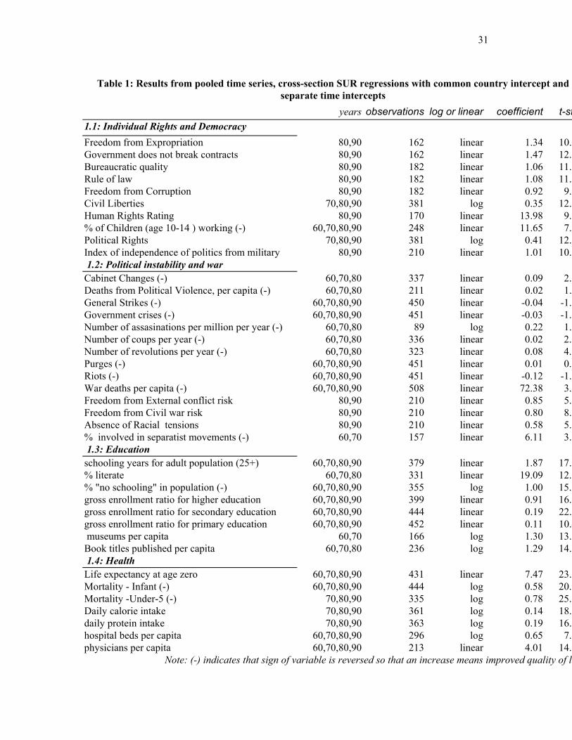
III. Results of SUR method in levels

Table 1 shows that 61 out of the 81 indicators display significant and positive effects of

income on the quality of life in levels, often with positive double-digit t-statistics (remember that

I take the minus of any variable where an increase indicates worse quality of life).

Rich countries compared to poor countries have more democracy, less corruption, less

expropriation of property, more contract-keeping by governments, more rule of law, and higher

bureaucratic quality. Rich countries compared to poor countries have more civil liberties, less

abuse of human rights, less use of child labor, more political rights, and more independence of

politics from the military. Rich countries compared to poor countries have fewer coups, cabinet

9

changes, and revolutions, less likelihood of civil or international war and less war deaths per

capita, less racial tension, and less separatism. 9 Rich countries compared to poor countries have

more museums, more average years of schooling, higher schooling enrollment ratios at all levels,

less illiteracy, less people with no schooling, and more book titles published per capita. Rich

countries compared to poor countries have greater life expectancy, fewer babies dying, less

children under 5 dying, more calorie and protein intake, more doctors, hospital beds, and nurses.

Rich countries compared to poor countries have more roads paved, more telegrams, telexes,

telephones, fax machines, radios, and TVs, fewer households without a toilet or clean drinking

water (including both rural and urban). Rich countries compared to poor countries have less

inequality between rich and poor, a smaller gap between men and women’s literacy, a smaller gap

between male and female enrollment ratios at all levels. Rich countries compared to poor

countries have less destruction of forest area, and less smoke in the air. The diversity of

indicators shown here to be positively associated with per capita income is greater than in any

previous study.

On the negative side, the “bads”, true to their name, show a negative effect of income on

the quality of life in eleven indicators. Some indicators of pollution, some crimes, injuries in the

workplace, and suicides get worse with higher income.10 Also road length per car (an indicator of

congestion of the road network) decreases with per capita income. So 12 of 81 indicators indicate

worsening quality of life with higher income. Only 8 of the 81 indicators of quality of life fail to

show a significant relationship with income, either positive or negative. These results indicate

very strong relationships between income and quality of life, which may either reflect a long run

causal relationship between income and quality of life, some reverse causality from quality of life

to income, or omitted fixed factors determining both income and life.

Although the income effects are strong, so is the exogenous time trend in many of the

quality of life indicators. Of the 61 quality of life indicators that show significant improvement

10

with growth, only 32 of them show a growth effect (at world mean growth) that is greater than the

exogenous improvement over time. Of the 12 indicators that showed a significant deterioration

with higher income, 11 of them have a positive exogenous improvement that partially offsets the

negative effects of higher income. These findings suggest that the previous literature, by focusing

on cross-section samples, overlooked the important role of exogenous global improvements in

quality of life indicators regardless of country incomes.

IV. Results controlling for country effects

Controlling for country effects has advantages and disadvantages. On one hand, it

removes any spurious correlation between income and quality of life that a third omitted factor

may have caused. On the other hand, sweeping out all the cross-section variation reduces the

range of variation of income and of the social indicators. Given that there is likely to be noise

from measurement error, this makes it harder to detect income effects on social indicators. If the

effects of income on quality of life occur with a long and variable lag, the results will be strong in

levels but weak controlling for country effects. I will argue that both the SUR levels results and

the results controlling for country effects should be taken seriously for a full picture of how the

quality of life evolves during growth.

I organize the results controlling for country effects by topic; each topic will have one

section in Table 2 and sometimes a graph. The sections show the statistics for each indicator and

for each estimation method. The patterns to look for are simply whether the relationship between

income and the quality of life indicator is significantly positive. At the end of this section, I will

do an overview of the patterns of significance of indicators.

1. Individual rights and democracy

Controlling for country effects, income coefficients for two democracy and rights

indicators are significant and positive in both the fixed effects and first differences-IV

regressions: child labor and government contract-keeping (Table 2). (Recall that I have changed

11

signs so that an increase in the variable always reflects improved quality of life.) One of the

institutional quality variables -- freedom from corruption -- have a significant and negative

relationship with income in both the fixed effects and first differences-IV results. The correlations

between income and civil liberties, political rights, and human rights do not show up here as

significant when the country fixed effects are removed.

Figure 1a shows the significant relationship in a scatter of the Humana human rights

index in levels against income. Figure 1b shows the non-relationship in deviations from time and

country averages. I will use here and in the following indicators a smoothing device to visually

inspect the data. I order the sample for indicator L by income. I calculate the average of indicator

L for the poorest 30 observations and the average of income for that same group, and plot that

point on a scatter diagram of indicator L against income. Then I move one observation and plot

the average of the group of observations 2 to 31 ordered by income. I keep doing this to get a

continuous stream of points until I get to the top 30 observations. Figure 1c shows the smoothed

data. Figures 1b and 1d show the unsmoothed and smoothed deviations from time and country

averages. This smoothing device is simply a moving average of 30 observations ordered by

income rather than by time. It closely resembles what the nonparametric literature calls a “k-

nearest neighbor estimator” of the typical y for a given x (see, for example, p. 42ff, Hardle

1990).)11 The dotted lines show the 2-standard deviation ranges for the means. I choose the scale

of the vertical axis of each graph to show the conceivable maximum and minimum that the

dependent variable could reach, unconditioned by income, in groups of 30 observations.12 This

helps us see how much y spans the range of variation of L. If the countries with the best (worst)

y are also the countries with the best (worst) L, then the heavy black line will hit the corners of

the box in each graph. Figure 1c shows the strong relationship in the smoothed data in levels.

Figure 1d shows the lack of relationship in smoothed data in deviations.

12

2. Political instability and war

None of the political instability or war measures are significant in both the fixed effects

and first differences-IV regressions (Table 2). In the fixed effect regressions, coups, revolutions,

and war deaths significantly improve with income.13 Absentees from a significant relationship

with income in fixed effects include racial tensions and prevalence of separatist movements,

which were strongly related to income in levels (see Table 1). Figure 2b with smoothed data

shows, for example, how little evidence there is for a relationship over time between income and

freedom from racial tensions after removing country effects, while figure 2a shows the strong

levels relationship.

3. Education

The relationship of education to income across countries has been firmly established in

the cross-section literature (as well as here in Table 1). However, none of the education variables

are positively and significantly related to income in both the fixed effects and first differences –

IV regressions(Table 2). Primary enrollment is actually negatively and significantly related to

income using both methods. (Pritchett (1997) shows a similar negative correlation in first

differences for enrollment ratios and income, although he is looking at income growth as the

dependent variable). The positive effects of income on average schooling years for the

population, college enrollment, and secondary enrollment do hold up under fixed effects.

Figures 3a and 3b illustrate again how different are the cross-section and the cross-time

results, in this case for literacy. Figure 3a shows the indisputable relationship between income

and literacy in the pooled cross-section, cross-time sample. Figure 3b shows the lack of

relationship in first differences. Recall that the range of values along the vertical axis represents

the maximum and minimum of the dependent variable. Figure 3b shows how none of this

variation is explained, in contrast to the levels chart where almost all the variation is explained.

13

To anticipate results on exogenous changes in social indicators, figure 3b also shows that the

growth in literacy was positive regardless of the growth rate of income.

4. Health

There are widely known relationships across countries between income and health

indicators such as infant mortality, under-5 mortality, and life expectancy, and many more (see

Table 1 again). Here, infant mortality, calorie intake, and protein intake are significantly and

positively related to income in both fixed effects and first differences – IV regressions.14

However, life expectancy’s relation to income is not positive and significant under either

fixed effects or first differences IV (see Table 2). Other variables simply are insignificant under

both methods, such as access to sanitation. Access to clean drinking water is also insignificantly

related to income under fixed effects. Hospital beds per capita, doctors per capita, and nurses per

capita are positively and significantly related to income under fixed effects, but not under first

differences – IV.

A monotonically negative relationship of infant mortality to income is strong in

deviations from time and country averages. The magnitude of the coefficient in fixed effects is in

the range that Filmer and Pritchett 1997 identified as common to most studies. Pritchett and

Summers 1996 present evidence that there is a causal relationship from income to infant

mortality. The first-differences IV results here confirm this finding.

5. Transport and communications

One would expect transport and communications (railroads, telegrams, telexes,

telephones, radios, TVs, faxes, percent roads paved) to go up strongly with income. Some of

these expectations are fulfilled. Such harbingers of civilization as telephones, telegrams, and TVs

are significantly positively related to income under both fixed effects and first differences IV

(Table 2). Although these are private rather than public goods, they are indicators of the degree to

which the government has invested in the public good of communications infrastructure.

14

Other relationships are more problematic. Romer 1990 treated radios in the cross section

as a variable so tightly linked to income that it could be used as an instrument for income

measured with error. Radios are positively and significantly related to income under fixed effects,

but negatively and significantly related to income under first differences.

Another notable absentee from the results is the percent of roads that are paved. In

contrast, the road length per car significantly declines according to the fixed effects estimator, as

it did in the levels regression (see Table 2).

6. Inequality across class and gender

The relation of inequality to income per capita has been intensively studied with a vast

literature seeking to confirm or reject the Kuznets curve. (For recent references, see Deininger

and Squire 1996 -- the source of my data here -- and Anand and Kanbur 1989). None of the

inequality indicators here are significant under both fixed effects and first differences IV. The

income share of the bottom quintile is positively related to income under first differences –IV, but

is of the opposite sign and insignificant under fixed effects. These non-results on income

inequality and income echo similar findings by Deininger and Squire 1996. 15 These results could

be seen as good news, because they contradict the fears of critics on the left that income

distribution would significantly worsen during growth.

As far as gender equality under fixed effects, female to male primary enrollment is

significant with the “wrong” sign with respect to income. Female to male secondary enrollment is

significant with the “right” sign. None of the gender equality measures are robust to the use of

the first differences IV estimator. Figures 4a and 4b show the absence of a relationship between

the female to male literacy ratio and income in first differences (4b), in contrast to the strong

relationship in levels (4a).

15

7. “Bads”

“Bads” are indicators that many consider a priori to be unwanted byproducts of higher

incomes. This section considers two principle types of “bads”: crime and the environment, as well

as some miscellaneous ones. Although the data on these indicators is poor, the strong interest in

them in the literature warrants some attempt to detect a relationship with income.

The relationship between crime and income is very weak in the fixed effects. The serious

problem of variation in reporting (in the UN Crime Survey) does not help this weak relationship.

The only crime to be significantly related to income (it worsens, in fixed effects) is manslaughter

(Table 2).16 I could interpret these weak results as good news if my prior was that crime worsened

with rising income. None of the crime indicators are significant under first differences IV.

The literature on per capita income and the other prominent “bad”-- pollution -- is already

extensive (see Grossman and Krueger 1993, Holtz-Eakin and Selden 1995, and Shafik 1995 for

important contributions). Here both the fixed effects and first-differences estimation shows that

the carbon emissions indicators (carbon dioxide and industrial carbon dioxide) and waste paper

production tend to get worse with income

The strong link between emissions and income here and elsewhere in the literature may

in part be an artifact of the way the source constructs emissions data.17 However derived, the

positive and significant coefficients on income for emissions of CO2 and industrial CO2 match

other results in the literature. Holtz-Eakin and Selden 1995 found a significant coefficient with an

IV fixed effects estimator on CO2.18

Grossman and Krueger 1993 used measures of ambient air quality instead of emissions

data. Unfortunately, the other ambient air quality measures and water quality measures that

Grossman and Krueger used did not have sufficient time or cross-section dimension for use in the

present study. However, there is one direct Grossman-Krueger measure of air quality with

sufficient data -- suspended particulate matter -- but it is not significantly related to income with

16

the fixed effects estimator. The annual change in forest area is likewise unrelated to income.

Finally, two very dissimilar “bads” – suicide and work injuries – are not significantly related to

income.19

8. Stock-Taking

How can we make sense of the large mass of material presented in Tables 1 and 2? There

is the good news that such core development indicators as child labor, infant mortality, nutritional

intake, and communications infrastructure are robustly related to income across countries and in

both fixed effects or first differences. The bad news is that other key modernization or

development indicators like democracy, good institutions, human rights, years of schooling,

school enrollment ratios, and life expectancy do not robustly improve with income controlling for

country effects and sometimes even have the wrong sign. Additional bad news is the robust

association of “bads” like CO2 emissions and waste paper production with growth.

One primitive means of summarizing the results is simply to count the number of

indicators where growth significantly betters welfare out of the total set of diverse indicators.

This is imperfect, since I can hardly assert that the indicators are independent Bernoulli trials of

some abstract quality of life concept. Still no alternative summary device is available. I will use

this one while reminding the readers it is preferable that they examine all of the information in

tables 1 and 2.

For the fixed effects estimator applied to 81 indicators, the coefficient of income was

significant at the 5% level for 34 indicators. Of these 34, 20 of them show improvement in the

quality of life associated with rising income. Fourteen indicators show significant deterioration in

quality of life as income rises. If we take the shortcut of regarding these as independent trials of

quality of life, we cannot reject the hypothesis that quality of life is equally likely to improve or

worsen with rising income (20 of 34 is not significantly greater than 50%).

17

The fixed effects estimator is appropriate if we simply want to chart the joint evolution of

income and “life,” or to discuss causal determination of “life” if income is exogenous. If income

is endogenous and we want to address causality, the first-differences IV estimator should be used.

Of the 69 indicators to which I applied this method20, income significantly affected 14 of them.

Six indicators of the quality of life significantly worsened with rising income -- corruption,

primary enrollment, radios, total CO2 emissions, industrial CO2 emissions, and waste paper

production. Eight out of the 69 indicators – government not breaking contracts, child labor,

calorie intake, protein intake, infant mortality, telephones, telegrams, and the share of the bottom

income quintile -- significantly improved with rising income. Again, we find that quality of life is

about equally likely to improve or worsen with rising income.

Although many of the associations between income and “life” in the SUR levels sample

are not robust to the use of fixed effects or first difference IV methods, I do not believe this

warrants discarding the SUR results. The SUR results in levels may still be capturing a long run

relationship between income (which is after all the sum of all past growth) and “life” (which is

the sum of all past social improvements). The weaker fixed effects and first differences IV results

may be reflecting the lack of a shorter-run contemporaneous relationship between income and

measured indicators of the quality of life.

9. Exogenous Changes in Quality of Life Indicators

I noted in section II that the estimation of separate time intercepts allows me to calculate

the “exogenous” change in each indicator. “Exogenous change” is the change in the indicator

over time holding income constant. (I put “exogenous” in quotes because these time shifts may

represent endogenous global innovation and may be a function of the global growth rate.)

Likewise, I can calculate the movement along the estimated indicator-income curve and derive

the “growth” contribution to the change over time in the indicator. I annualize in percent both the

“exogenous change” and the “growth effect." This allows me to assess the relative importance of

18

growth and exogenous change in movements in the indicator. I do this for the fixed effects

estimator.

Table 3 shows the results for all 81 indicators for the fixed effects estimator. Note first

that the time shifts are very important for some variables (* indicates significant at 5%), even

though we might have worried that such shifts would be imprecisely estimated with time periods

as short as a decade. Moreover, most of the time shifts (51 out of 81 indicators) improve quality

of life.

How does the exogenous time shift effect compare to the growth effect for each

indicator? I will use the same kind of crude indicator count as before. With the Fixed Effects

estimator, time shifts were more important than growth effects for 67 percent of the indicators. 21

I did this exercise also for the First Differences IV estimator. In the sample of 69

indicators available for the First Differences indicator, 62 percent of the indicators had time shifts

improve the indicator more than growth did (not shown but available upon request). For example,

even a variable as strongly related to income as infant mortality declined more from exogenous

change over time (-1.6% per year) than from rising income (-0.9% per year).

I combine this result with the previous results on significance of income. I noted before

that 20 out of 81 quality of life indicators had a significantly positive relationship with income

under fixed effects. Time improved 10 of these 20 indicators more than income did. The 10 that

had growth dominate with a significant positive sign are: a government that does not break

contracts, child labor, coups, revolutions, war deaths per capita, calorie intake, protein intake,

hospital beds, telephones, and mail. Under the first differences estimator, 6 out of 69 indicators

had a positive, significant relationship with income that was more important than exogenous

change: government does not break contracts, calorie intake, protein intake, telephones,

telegrams, and the share of the bottom income quintile. Of these six, telegrams and the share of

the bottom income quintile were not in the fixed effects list but the other four were. With the

19

SUR estimator, the indicator “government does not break contracts” has an exogenous trend

stronger than the growth effect. So there are three variables robust to all three estimators for

which growth is the primary life-improving and significant determinant: calorie intake, protein

intake, and telephones.

V. Robustness Checks

In this section, I perform a number of robustness checks. I check first-stage regressions,

apply some non-parametric tests, check for nonlinearities, and consider the special case of the

fast-growing East Asian economies.

One might worry that the IV coefficient estimates on income will be very imprecise if the

first stage regression was a poor fit. I have first-stage R-squareds of .32, .23, .23, .10, and .10 for

the first stage regressions in the different time periods 60,70,80,90; 80,90; 70,80,90; 70, 80; and

60,70,80. The F-statistic is insignificant only in the last two regressions (actually the same

regression given the use of income lagged two periods) for 70,80 and 60,70,80. There are 12

indicators run in first differences -IV that belong to these problematic time periods; only one of

them is significant. The estimates for the other time periods seem to be on firmer ground.

Next, I expand the length of period from 10 years to 30 years. Perhaps the decade data

are so noisy as to obscure the temporal association of life with growth. How did growth of

income over thirty years causally affect the growth of quality of life indicators? I run IV on the

25 indicators that have the requisite data, using the policy indicators as instruments (first stage

R2=.29).22 The results (not shown) have a familiar ring: 4 of the 25 indicators are significant

with the “right” sign and 4 with the “wrong” sign. The identity of the “good” significant

indicators is also familiar: child labor, infant mortality, phones, and TVs.

As another robustness check, I use a non-parametric test of whether a country that moved

up (down) in the ranks of income also moved up (down) in the ranks of the social indicator from

1960 to 1990. I do a simple signs test for whether the sign of the change in the ranking of the

20

social indicator matched that of the change in income ranking. Six of the 25 variables showed a

positive association between the change in rank in income from 1960 to 1990 and the change in

rank of the quality of life indicator. Four showed a negative association. Such standard

development indicators as female literacy, life expectancy, primary and secondary enrollment,

and the share of population with no schooling failed to show improvement with rising income

according to this method.

1. Nonlinearities

Next, I check directly whether there were pronounced nonlinearities that might have

caused the specifications (1) and (2) to be seriously misspecified. The quality of life literature

sometimes postulates a U-shaped or inverted U-shaped function of y for L. Could it be that a zero

average relationship obscures a path in which quality of life falls (rises) and then rises (falls) with

rising income?

I split the sample for the first-differences IV regression into the portions above and below

the whole sample mean across countries. If there were a pronounced U-shape, the coefficient on

income growth in this regression should change sign from low to high income. I perform this

exercise using both the log-change and linear-change specifications for the dependent variable.

As it turns out, there are only two variables that have significant coefficients of opposite

sign between low and high income. The linear change in doctors per capita is negatively and

significantly related to income growth at below-average incomes and positively and significantly

related to growth at above-average incomes. The change in primary school enrollment is

positively associated with growth at below average incomes and negatively associated at above

average incomes.

I perform a similar exercise for the fixed effects estimator by adding a quadratic term in

the log of initial income to the FE regression. The quadratic term will eventually become

dominant so its sign and significance indicate what will eventually happen to the dependent

21

variable as income rises (the turning points with significant quadratic terms were generally well

within the sample range). There were seven indicators that did not significantly improve with

growth under the linear specification that do show significant eventual improvement under the

quadratic specification (a right-side-up U). However, what the quadratic giveth, the quadratic

also taketh away. There were seven indicators that did show improvement under the linear

specification that show a significant eventual deterioration under the quadratic specification (an

upside down U). There is little evidence that the existence of U-curves is responsible for the low

number of quality of life indicators that are positively and significantly related to income under

fixed effects.

Note that the quadratic function of income could also capture a monotonic relationship

that is concave or convex. This would show up if the turning point in income were close to the

endpoints of the income range. Infant mortality, child labor, and mail per capita show a

relationship in which there is not much improvement at low income but there is much more at

higher incomes. Carbon dioxide emissions, sulfur dioxide emissions, war deaths, and the ratio of

females to males for higher education show a relationship to income in which there is a strong

change at lower levels of income that tails off at high incomes. (All these results are of the same

sign as in the original fixed effects results). The limited number of variables in which concave or

convex relationships hold, and with most of these having the same sign and significance as in the

fixed effects results, suggest that convexity or concavity of the income-social indicator

relationship does not change the basic story.

I next consider whether the existence of some bounded variables may have contributed to

the poor results with the linear or log-linear results. I do two monotonic transformations in fixed

effects of those L variables bounded between zero and one. First, I use the inverse logistic

function L/(1-L), which maps the [0,1] variable into [0,∞]. This transformation implies that y will

have a strong effect on L at low incomes, but progressively smaller effects at higher incomes.

22

Second, I use the negative reciprocal function, -1/L, which maps the [0,1] variable into [-∞,-1].

The negative reciprocal transformation implies that L will hardly improve at low incomes but will

improve much at high incomes. I apply these transformations to all the variables that are bounded

between zero and one and actually range between zero and one in the sample. These variables are

% literate, % no schooling in population, enrollment ratios for primary and secondary education,

% with access to clean drinking water (total, rural, and urban), and % with access to sanitation

(total, rural, and urban). Of these, the only one where income becomes positive and significant in

either of the two functional forms is % rural with access to clean drinking water (negative

reciprocal functional form).

I apply a related functional transformation to the first differences IV regression. I

estimate the improvement in the L variable as a ratio to the maximum possible improvement:

(L-L(-1))/(1-L(-1)).23 The only variable to become significant in differences in this functional

form is the enrollment ratio for secondary education.

Another type of nonlinearity might be irreversibility of social indicators. Some indicators

may improve with growth, but not symmetrically worsen with negative growth (for example,

roads paved and railroad mileage). I checked this by introducing intercept and slope dummies for

observations in which decade growth was negative.24 The only indicators that support the

irreversibility argument (having a significantly lower coefficient when growth is negative) are the

ratio of females to males in higher education, hospital beds, and literacy. However, the coefficient

on the positive change in income is not significantly different from zero for these three indicators.

I conclude that irreversibility is not a major factor in the evolution of social indicators.

2. Changes in Quality of Life Indicators in Fast Growing East Asian Economies

It may be that we fail to detect consistent changes in the quality of life with income

because income has not grown very much in many economies. Another robustness check I can

perform is to look at the subset of rapidly growing economies. I choose the countries covered in

23

the World Bank’s East Asian Miracle – Hong Kong, Indonesia, Japan, Korea, Malaysia,

Singapore, Taiwan, and Thailand (other high growth economies like Botswana and Lesotho have

poor data availability). To summarize a large amount of information, I use the device of

examining the change in percentile rank of each country for each indicator from 1960 to 1990.

This automatically controls for the global shift in level of each indicator from 1960 to 1990. As

shown in Table 4, each of the East Asian miracles moved up by around a quartile in the income

ranking from 1960 to 1990. Did they have some similarly large upward movements in the

rankings of the quality of life indicators?

Table 4 shows the results for individual indicators and countries. There are some notable

successes: the reduction in the unschooled population in Japan (shown with sign reversed), the

increase in life expectancy and reduction in infant mortality in Japan, the rise in hospital beds in

Korea and Thailand, the increase in TVs in Indonesia and Malaysia, the increase in radios in

Indonesia and Korea, the change in telephones in Korea, and the increase in female to male

average schooling years in Indonesia. However, another thing to note is the number of negative

signs (here as elsewhere I change the sign of each indicator so that increase means improved

quality of life). Out of 141 entries, 70 are negative – indicating that the East Asian miracles have

moved down in the rankings on quality of life indicators about as often as they have moved up.

This seems to reinforce the finding from the first difference regressions that there is not a strong

tendency for positive changes in quality of life to be associated with positive changes in income.

Examining individual countries, we see that Korea is the only one with a median strong

upward movement in quality of life rankings. Examining individual indicators, we see that goods

that have a strong private good element –telephones, TVs, and radios – do show a strong upward

movement with East Asian growth. There are a couple other indicators that show strong

improvement – nurses and ratio of female to male enrollment for secondary education. However,

24

the median change in percentile ranking in the quality of life indicators is just 3 percentage

points.

Figure 5 gives the example of the higher education indicators – both total enrollment and

equality between men and women. With total higher education enrollment, three of the tigers –

Japan, Taiwan, and Thailand – had faster increases than the world median, but four other tigers

had slower increases than the world median despite their faster GDP growth. On the ratio of

women to men in higher education, which was significantly related to income in the SUR levels

regressions, all of the tigers except Singapore have a slower increase than the world median.

(Singapore almost exactly follows the world median, which was why it is hard to distinguish in

the graph.)

V. Conclusions

How can the cross-time growth effects be so weak when the cross-section, cross-time

income effects are so strong? I believe both findings should be taken seriously, so we need a story

of how there could be a strong cross-country relationship but a weak cross-time relationship.

Note first of all that worsening income distribution, as hypothesized by many critics of

growth, is not the operative mechanism. There is no evidence here that income distribution

worsens during growth; actually, there is some evidence that the share of the poor in national

income gets better with growth. So what accounts for the strong cross-section cross-time findings

but weak cross-time results?

The most prosaic possibility is that the methods of fixed effects and first differences

simply remove too much of the signal and leave too much of the noise. The noise may come

from measurement error or just from temporary shocks to income or the quality of life indicator.

Detecting the signal is less likely once one removes the large cross-section differences in income.

However, note that the failure to pick up large quality of life improvements in the fast-growing

East Asian is evidence against this view. Moreover, even if measurement error is the problem,

25

these results are important to show us the limitations of our knowledge on the contemporaneous

link between growth and changed quality of life.

There is a related and plausible possibility. Perhaps long and variable lags and the lack of

sufficiently long time series prevent the detection in decade changes of the true relationship

between life and growth. Recall from the economic history literature on the now-rich nations the

documentation of episodes of declining quality of life indicators while per capita income was

rising. This historical evidence may reflect the long lags between income growth and quality of

life improvements. Similarly for our sample, past growth and social investment over many

decades may have been one of the “fixed factors” that was differenced out in the fixed effects and

first differences methods. The cross-section may contain the true long-run relationship after all,

while the fixed effects and first differences methods just showed the weak contemporaneous part

of a long lag structure.

A more fundamental change from conventional wisdom would be that fixed factors really

could be the dominant determinant of a country’s income and quality of life indicators. As

already noted, such fixed factors could include: a country’s resource endowments, access to the

sea, ethnic fragmentation, social infrastructure, climate, and legal systems. These factors would

create a spurious correlation in the cross section, which would be correctly removed in the fixed

effects and first differences methods.

Another possibility is that, since the main criterion for selecting these indicators was that

they were at least partially public goods, there is a public goods problem during growth. A rise in

private incomes (per capita GDP) does not necessarily translate into increased public goods. John

Kenneth Galbraith made a famous argument to this effect for the 1950s US in his Affluent

Society.

Finally, there is the credible possibility that changes in the home country’s quality of life

indicators depend as much on changes in world income as on changes in home country growth.

26

For example, the improvement in life expectancy everywhere may have reflected technical

breakthroughs in antibiotics associated with world economic growth. The strong results on the

exogenous time shifts, even in the SUR levels regressions, point in this direction.

In conclusion, the evidence that life gets better during growth is surprisingly uneven,

while the cross-country relationship between income and diverse indicators of the quality of life

remains strong.

27

Bibliography

Anand S. and S.M.R. Kanbur, 1993, Inequality and development: a critique, Journal of Development Economics 41: 19-43.

Baltagi, Badi H., 1995, Econometric Analysis of Panel Data, Wiley: New York. Barro, Robert and Xavier Sala-i-Martin, 1995, Economic Growth, McGraw-Hill: New York. Barro, Robert. 1996. “Democracy and Growth”, Journal of Economic Growth 1(1): 1-27. Barro, Robert, 1997, Determinants of Economic Growth: A Cross-Country Empirical Study, MIT Press, Cambridge

MA. Barro, Robert and Jong-wha Lee, 1997, “Determinants of schooling quality,” mimeo, Harvard and Korea Universities. Baumol, William J., Sue Anne Batey Blackman, and Edward N. Wolff, Productivity and American Leadership: the

Long View, MIT Press, 1989 Bennett, Richard R., 1991, “Development and crime: A cross-national, time-series analysis of competing models,” The

Sociological Quarterly 32(3): 343-363. Boone, Peter, 1996, “Political and gender oppression as a cause of poverty,” mimeo, London School of Economics,

April. Brandt Commission, 1980, North-South: A Programme for Survival. (London: Pan Books) Bruno, Michael and William Easterly, “Inflation Crises and Long-run Growth,” Journal of Monetary Economics,

February 1998. Clague, Christopher, Philip Keefer, Stephen Knack, and Mancur Olson, 1996, “Property and Contract Rights in

Autocracies and Democracies,” Journal of Economic Growth 1(2): 243-276. Dasgupta, Partha and Martin Weale, 1992, “On measuring the quality of life,” World Development 20(1):119-131. Dasgupta, Partha. 1993. An Inquiry into the Sources of Well-Being and Destitution. Oxford: Clarendon Press Deininger, Klaus and Lyn Squire, “A New Dataset Measuring Income Inequality.” The World Bank Economic

Review10(3): 565-91, September 1996 Easterlin, Richard A. 1996. “Does Satisfying Materal Needs Increase Human Happiness?”, Chapter 10 in Richard A.

Easterlin, Growth Triumphant: The Twenty-First Century in Historical Perspective (Ann Arbor: University of Michigan Press).

Easterly, W. and R. Levine, 1997, “Africa’s Growth Tragedy: Policies and Ethnic Divisions, Quarterly Journal of

Economics, Volume CXII, Issue 4 (November), 1203-1250. Fahnzylber, Pablo, Daniel Lederman, and Norman Loayza, “What Causes Violent Crime?”, Office of the Chief

Economist, Latin America Region, World Bank, mimeo, 1998 Fedderke, Johannes and Robert Klitgaard, 1998, “Economic growth and social indicators: An exploratory analysis,” ECONOMIC DEVELOPMENT AND CULTURAL CHANGE 46:455-89, April. Filmer, Deon and Lant Pritchett Child mortality and public spending on health : how much does money matter?

Washington, DC : World Bank, Policy research working paper 1864, December 1997. Fogel, Robert W., 1994, “Economic Growth, Population Theory, and Physiology: the Bearing of Long-term Processes

on the Making of Economic Policy,” American Economic Review 84(3): 369-395. Fogel, Robert W. 1990. “The Conquest of High Mortality and Hunger in Europe and America: Timing and

Mechanisms,” NBER Working Paper Series on Historical Factors in Long Run Growth No. 16, September.

28

Greene, William H., 1997, Econometric Analysis, (Prentice Hall: Upper Saddle River NJ) Griliches, Zvi and Jerry Hausman, 1986, “Errors in Variables in Panel Data,” Journal of Econometrics 31: 93-118. Grossman, G.M. and Krueger, A. B. 1993 “Environmental impacts of a North American free trade agreement,” in P.

Garber, ed., The US Mexico Free Trade Agreement, Cambridge: the MIT Press, 165-177. Hall, Robert E. And Charles I. Jones, “Levels of Economic Activity Across Countries,” AMERICAN ECONOMIC

REVIEW, PAPERS AND PROCEEDINGS 87, No. 2:173-177, May 1997 Hall, Robert E and Charles I. Jones, “Why do some countries produce so much more output than others?”, Stanford

University mimeo, March 1998. Hamermesh, Daniel S. and Neal M. Soss, 1974, “An economic theory of suicide,” Journal of Political Economy 82(1):

83-98. Hardle, Wolfgang. 1990. Applied Nonparametric Regression. Cambridge: Cambridge University Press. Helliwell, John F., 1992, “Empirical linkages between democracy and economic growth,” NBER Working Paper 4066,

May. Holtz-Eakin, Douglas and Thomas Selden, 1995, “Stoking the Fires: CO2 Emissions and Economic Growth,”

JOURNAL OF PUBLIC ECONOMICS 57:[85]-101 May. Huntington, Samuel, 1968, Political Order in Changing Societies, New Haven: Yale University Press. Huntington, Samuel, 1987, “The Goals of Development”, in Myron Weiner and Samuel P. Huntington, eds.,

Understanding Political Development, Boston: Little Brown and Company Independent Commission on Population and the Quality of Life, 1996, Caring for the Future. Oxford: Oxford

University Press. Galbraith, John Kenneth. 1958. The Affluent Society. (Boston: Houghton Mifflin) Kakwani, N., 1993, “Performance in living standards: an international comparison,” Journal of Development

Economics 41: 307-336. Knack, Stephen, and Philip Keefer, 1995, “Institutions and Economic Performance: Cross-country tests using

Alternative Institutional Measures,” Economics and Politics, Vol. 7, No. 3, 207-228. Knack, Stephen and Philip Keefer, 1997, “Does social capital have an economic payoff? A cross-country

investigation,” Quarterly Journal of Economics, November. La Porta, Rafael, Florencio Lopez-de-Silanes, Andre Shleifer and Robert Vishny, 1998a, “Law and Finance,” Journal-

of-Political-Economy 106(6), December, pages 1113-55. La Porta, Rafael, Florencio Lopez-de-Silanes, Andre Shleifer and Robert Vishny, 1998b, “The quality of government,”

NATIONAL BUREAU OF ECONOMIC RESEARCH WORKING PAPER SERIES No. 6727, September Lewis, W. Arthur, 1955, The Theory of Economic Growth (Irwin: Homewood, IL) Lindert, Peter H. and Jeffrey G. Williamson, “English Workers’ Living Standards During the Industrial Revolution: A

New Look”, The Economic History Review, Second Series, Volume XXXVI, No. 1, February 1983, pp. 1-25. Lipset, Seymour M., 1959, “Some social requisites of democracy: economic development and political legitimacy,”

The American Political Science Review 53(3), 69-105. Londregan, John B. and Keith T. Poole, 1990, “Poverty, the coup trap, and the seizure of executive power” World

Politics 42: 151-83.

29

Londregan, John B. and Keith T. Poole, 1996, “Does high income promote democracy?” World Politics 49(1): 1-30 Mauro, Paolo, 1995, “Corruption and Growth,” Quarterly Journal of Economics, 110(3): 681-712. Morris, Cynthia Taft. “How fast and why did early capitalism benefit the majority?” The Journal of Economic History,

Volume 55, Number 2, June 1995, pp. 211-226. Morris, Morris David. 1979. Measuring the condition of the world's poor : the physical quality of life index (New York : Published for the Overseas Development Council by Pergamon Press) North, Douglas. 1990. Institutions, Institutional Change, and Economic Performance (Cambridge: Cambridge

University Press). Oak Ridge National Laboratory, 1989, Estimates of CO2 Emissions from Fossil Fuel Burning and Cement

Manufacturing, ORNL/CDIAC-25, NDP-030, May. O’Kane, Rosemary, 1983, “Towards an examination of the general causes of coups d’etat,” European Journal of

Political Research, 11: 27-44. Polak, Ben and Jeffrey G. Williamson, “Poverty, policy, and industrialization: lessons from the distant past,” World

Bank Working Paper 645, April 1991. Preston, Samuel H., 1976, “The changing relationship between mortality and level of economic development,”

Population Studies 29:2: 231-247. Pritchett, Lant and Larry Summers, 1996, “Wealthier is Healthier,” Journal of Human Resources, 31(4): 841-68 Pritchett, Lant. 1997. “Where has all the Education Gone?”, World Bank Working Paper. Rahav, Giroa and Shiva Jaamdar, “Development and crime: a cross-national study,” Development and Change 13(4),

447-462. Ram, Rati 1985, “The role of real income level and income distribution in fulfillment of basic needs,” World

Development 13: 589-594. Ravallion, Martin, 1990, “Income effects on undernutrition,” Economic Development and Cultural Change 38: 489-

516. Ravallion, Martin, 1992, “Does undernutrition respond to incomes and prices? Dominance tests for Indonesia,” World

Bank Economic Review 6(1):109-124. Ravallion, Martin and Shaohua Chen, 1997, “What can new survey data tell us about recent changes in distribution and

poverty?”, The World Bank Economic Review 11(2): 357-82. Romer, Paul M. 1990. “Human Capital and Growth: Theory and Evidence.” Carnegie-Rochester Series on Public

Policy 32 (1990): 251-86. Sachs, Jeffrey D. and Andrew Warner, 1995, Natural resource abundance and economic growth. NATIONAL BUREAU

OF ECONOMIC RESEARCH. WORKING PAPER SERIES, No. 5398:1-47, December Sachs, Jeffrey D. and Andrew Warner, 1997, “Fundamental sources of long-run growth.” AMERICAN ECONOMIC

REVIEW, PAPERS AND PROCEEDINGS 87, No. 2:184-88, May. Sen, Amartya, 1994, “Economic regress: concepts and features,” Proceedings of the World Bank Annual Conference

on Development Economics, 315-330. Shafik, Nemat, 1994, “Economic development and environmental quality: an econometric analysis,” Oxford Economic

Papers 46:757-73 October Todaro, Michael P. 1997. Economic Development. 6th edition, Longman: New York.

30

United Nations Development Program, 1996, Human Development Report. United Nations Environment Program Yearbook 1994 Unithan, N. Prabha and Hugh P. Whitt, 1992, “Inequality, Economic Development, and Lethal Violence: A Cross-

national analysis of Suicide and Homicide,” International Journal of Comparative Sociology 33 (4), 182-196.

Wallerstein, Immanuel, 1976, “Modernization: Requiescat in Pace”, in Lewis A. Coser and Otto N. Larsen, eds., The

uses of controversy in sociology, New York: Free Press. Weede, Erich, 1981, “Income inequality, average income, and domestic violence,” Journal of Conflict Resolution

25(4): 639-654. Wheeler, David 1980, “Basic needs fulfillment and economic growth: a simultaneous model,” Journal of Development

Economics 7: 435-451. Williamson, Jeffrey G. “Was the Industrial Revolution worth it? Disamenities and Death in 19th Century British

towns.” Explorations in Economic History 19, 221-245 (1982) Wolfe, Barbara and Jere Behrman, 1983, “Is income overrated in determining adequate nutrition?,” Economic

Development and Cultural Change 31: 525-549.

31

Table 1: Results from pooled time series, cross-section SUR regressions with common country intercept and

separate time intercepts years observations log or linear coefficient t-st

1.1: Individual Rights and Democracy Freedom from Expropriation 80,90 162 linear 1.34 10.7Government does not break contracts 80,90 162 linear 1.47 12.7Bureaucratic quality 80,90 182 linear 1.06 11.3Rule of law 80,90 182 linear 1.08 11.0Freedom from Corruption 80,90 182 linear 0.92 9.6Civil Liberties 70,80,90 381 log 0.35 12.2Human Rights Rating 80,90 170 linear 13.98 9.9% of Children (age 10-14 ) working (-) 60,70,80,90 248 linear 11.65 7.7Political Rights 70,80,90 381 log 0.41 12.5Index of independence of politics from military 80,90 210 linear 1.01 10. 1.2: Political instability and war Cabinet Changes (-) 60,70,80 337 linear 0.09 2.3Deaths from Political Violence, per capita (-) 60,70,80 211 linear 0.02 1.2General Strikes (-) 60,70,80,90 450 linear -0.04 -1.9Government crises (-) 60,70,80,90 451 linear -0.03 -1.2Number of assasinations per million per year (-) 60,70,80 89 log 0.22 1.Number of coups per year (-) 60,70,80 336 linear 0.02 2.9Number of revolutions per year (-) 60,70,80 323 linear 0.08 4.5Purges (-) 60,70,80,90 451 linear 0.01 0.8Riots (-) 60,70,80,90 451 linear -0.12 -1.2War deaths per capita (-) 60,70,80,90 508 linear 72.38 3.3Freedom from External conflict risk 80,90 210 linear 0.85 5.7Freedom from Civil war risk 80,90 210 linear 0.80 8.5Absence of Racial tensions 80,90 210 linear 0.58 5.7% involved in separatist movements (-) 60,70 157 linear 6.11 3.3 1.3: Education schooling years for adult population (25+) 60,70,80,90 379 linear 1.87 17.6% literate 60,70,80 331 linear 19.09 12.3% "no schooling" in population (-) 60,70,80,90 355 log 1.00 15.gross enrollment ratio for higher education 60,70,80,90 399 linear 0.91 16.6gross enrollment ratio for secondary education 60,70,80,90 444 linear 0.19 22.3gross enrollment ratio for primary education 60,70,80,90 452 linear 0.11 10.4 museums per capita 60,70 166 log 1.30 13.5Book titles published per capita 60,70,80 236 log 1.29 14.9 1.4: Health Life expectancy at age zero 60,70,80,90 431 linear 7.47 23.Mortality - Infant (-) 60,70,80,90 444 log 0.58 20.6Mortality -Under-5 (-) 70,80,90 335 log 0.78 25.7Daily calorie intake 70,80,90 361 log 0.14 18.0daily protein intake 70,80,90 363 log 0.19 16.2hospital beds per capita 60,70,80,90 296 log 0.65 7.7physicians per capita 60,70,80,90 213 linear 4.01 14.3

Note: (-) indicates that sign of variable is reversed so that an increase means improved quality of li

32

years observations log or linear coefficient t-st1. 4: Health (continued) nurses per capita 60,70,80,90 95 linear 11.63 8.4% with access to safe water 70,90 144 linear 20.57 10.3% rural with access to safe water 70,90 143 linear 17.87 7.% urban with access to safe water 70,90 152 linear 11.10 5.5Access to sanitation 70,80,90 202 linear 22.94 15.6Access to sanitation (rural) 80,90 142 linear 21.80 10.0Access to sanitation (urban) 80,90 151 linear 15.66 8.9 1.5: Transport and Communications Paved Roads as share of all Roads 80,90 228 linear 17.24 10.6Road length per car 60,90 132 log -0.93 -11.9Railroad Mileage per square mile 60,70,80 289 log 0.72 7.3Telephones per capita 60,70,80,90 364 log 1.53 31.6International telexes, minutes per capita 80,90 134 log 0.91 4.8telegrams per capita 70,80,90 156 log 0.75 7.0Radios per capita 60,70,80,90 440 linear 0.82 20.2TVs per capita 60,70,80,90 362 log 1.79 23.2Mail Per capita 60,70 184 log 1.66 17.Fax machines per capita 80,90 105 log 1.84 18.6 1.6: Inequality across class and gender Gini coefficient (-) 60,70,80,90 193 linear 3.41 4.4Share of income of bottom 20% 60,70,80,90 157 linear 0.00 0.5Share of income held by middle 60% 60,70,80,90 157 linear 0.03 5.5Share of income of top 20% (-) 60,70,80,90 157 linear 0.03 4.9Female to male schooling years (age 26+) 60,70,80,90 375 linear 0.14 9.7Ratio of Women's Literacy to Men's 60,70,80,90 294 linear 13.12 6.3Female to male primary enrollment 60,70,80,90 390 linear 0.09 9.6Female to male secondary enrollment 60,70,80,90 374 log 0.28 12.Female to male higher enrollment 60,70,80,90 350 log 0.43 14.6 1.7: "Bads" Fraud rate per capita (-) 70,80,90 143 log -1.22 -8.3Freedom from Political terrorism (-) 80,90 210 linear -0.63 -6.2Homicide rate per capita (-) 70,80,90 141 linear 0.41 0.7manslaughter per capita (-) 70,80,90 104 linear 1.77 3.4Robbery rate per capita (-) 70,80,90 148 log -0.21 -1.2Rapes per capita (-) 70,80,90 145 log -0.37 -2.9Drug crimes per capita (-) 70,80,90 139 log -1.04 -5.8Carbon Dioxide Emissions per capita (-) 60,70,80,90 469 log -1.47 -32.4Industrl CO2 Emissions Per Capita (-) 70,80,90 375 log -1.45 -32.3Sulphur Dioxide Emissions per capita (-) 70,80,90 91 log -1.23 -9.4Nitrogen Oxides Emissions per capita (-) 70,80,90 107 log -1.10 -16.7Suspended particulate matter (-) 70,80 55 log 0.69 6.9Annual forest area change (%) 60,70,80 343 linear 0.00 4.0Waste paper production per capita (-) 60,70,80,90 191 log -1.68 -18.0Injuries at work (per 1000 workers) (-) 80,90 110 log -1.46 -10.9Suicides per capita (-) 70,80 61 log -0.53 -3.0Note: (-) indicates that sign of variable is reversed so that an increase means improved quality of life

33

34

35

Endnotes

1 p. 453, Barro and Sala-i-Martin 1995 2. Huntington was characterizing the viewpoint of the 60s from the vantage point of the 80s. 3 Wallerstein 1976. 4 The most well-known critic of GDP growth is the Human Development Report of the United Nations Development Program, the 1996 issue of which opened with: “The purpose of growth should be to enrich people’s lives. But far too often it does not.” The Brandt Commission of 1980 warned against the “persistent confusion of growth with development.” The 1994 Independent Commission on Population and the Quality of Life concluded that “GNP proves to be an inadequate road-map for the quality of life,” a conclusion the authors thought was so important that they repeated the sentence four separate times. The usual concern underlying these sentiments is that income distribution worsens during growth, so that the majority of the population experience no benefits. 5 Exceptions are Kakwani 1993, Sen 1994, Dasgupta and Weale 1992 and Pritchett and Summers 1995, but they all concentrate on one or a handful of indicators. Conversely, there is a literature on quality of life over time based on a small number of rich countries (e.g. Baumol et al. 1989, Fogel 1994). Finally there is Fedderke and Klitgaard 1998, who do have a diverse set of indicators but have no time dimension. 6 This project gathered data first from several large cross-national databases available: the World Bank’s BESD data collection, Political Risk Services data, Banks 1994, Deininger and Squire 1996, Taylor and Jodice 1983, Barro and Lee 1996, various United Nations publications, and the World Resources Institute 1994. (See Appendix 1 for a full list of sources.) Secondly, I used data from more specialized sources discovered in a literature search over the categories mentioned. Where multiple versions were available of the same indicator were available, I chose the one with the largest number of observations -- other things equal -- and I preferred original sources over secondary sources. When I had two slightly different measures of the same general phenomenon, I keep the one I judge to be closer to “quality of life” and discard the other. 7 I have an unbalanced panel because of uneven data availability by dates. I estimate (1) with the Least-Squares Dummy Variable method discussed by Greene 1997 and Baltagi 1995, i.e. simply running OLS on yit with dummy variables for the λt and µi. 8 The direct source for the first two is Easterly and Levine 1997. The source for inflation is Bruno and Easterly 1998. 9 Fedderke and Klitgaaard 1998 also found rights, institutional efficiency, political stability, and absence of separatism to improve with per capita income. 10 The positive correlation between crime and income, or between suicide and income may reflect greater reporting in high-income societies. 11 The only difference between this moving average over income and the k-nearest neighbor estimator is that the former averages over the k nearest in rank, while the latter averages over the k nearest in distance. 12 I calculated this by ordering the sample by the dependent variable and showing the mean dependent variable value for the top 30 and the bottom 30. 13 Other social scientists, such as O’Kane 1983 and Londregan and Poole 1990, have noted the negative cross-national relationship between income per capita and coups, albeit without controlling for country fixed effects. 14 Microeconomic studies have shown the connection between income and nutrition (Ravallion 1992,1990). Wolfe and Behrman 1983 show that it weakens if they introduce other controls such as mother’s knowledge of nutrition (correlated with income -- here’s the partial-total problem once again). 15 I do not have enough data to estimate a relationship between absolute poverty and income. Ravallion and Chen 1997 find a relationship between the increase in mean consumption and the reduction in poverty in a survey panel data set. 16 Note that most of the data here are from the upper national income quintiles, so we cannot say what is happening at the bottom 1, 2 or even 3 quintiles. The previous literature also showed an ambiguous relationship between crime and income, although again focusing on partial correlations and the cross-section. Rahav and Jaamdar 1982 for example found a positive partial correlation of theft with income and a negative relation of homicide to income. But they were controlling for factors strongly correlated with income such as urbanization, mass communication, transportation, and education. Bennett 1991 looks at INTERPOL cross-country crime statistics. He finds evidence for income per capita raising theft rates but not affecting homicide. His equation includes a number of other control variables. Unnithan and Whitt 1992 find no relationship between homicide and per capita income in a cross-national study. Fajnzylber, Lederman, and Loayza 1998 find no robust link between homicide/robbery and per capita income, either using cross-section or dynamic panel methods. 17 According to the United Nations Environment Program 1994, staff estimated carbon dioxide emissions based on UN consumption data for gases, liquids and solid fuels plus cement manufacturing -- not bad proxies for GDP. They then apply “appropriate emission factors (P. 34).” Oak Ridge National Laboratory 1989 (the source of the UN

36

methodology) confirms that these “appropriate emission factors” are applied as constants for each type of fuel (and for cement manufacturing) across countries and across time. 18 These authors find evidence of quadratic turning points, but they are at very high income levels. Shafik 1994 finds an extremely strong relationship between income and CO2 emissions without correcting for country effects. 19 Unnithan and Whitt 1992 find that suicide is not significantly correlated with income across nations. Hamermesh and Soss 1974 used micro data and found the sign of the income-suicide relation to be generally negative. There may be differences across cultures in the propensity to report suicides. 20 The other indicators did not have data for 80 or later, which is required for this method using income lagged two periods, or were missing data on the instruments making the sample too small. 21 Preston 1976 found that 16 percent of the rise in life expectancy from the 1930s to the 1960s was due to per capita income growth, while 84 percent was due to exogenous time shifts. 22The 25 indicators are child labor, strikes, government crises, purges, riots, war deaths per capita, average years of schooling, percent with no schooling, higher education enrollment, secondary enrollment, primary enrollment, life expectancy, infant mortality, hospital beds, doctors per capita, telephones per capita, radios per capita, TVs per capita, the Gini coefficient, ratio of average years of schooling for females to that for males, female literacy, ratio of female to male primary enrollment, ratio of female to male secondary enrollment, ratio of female to male higher educational enrollment, and carbon dioxide emissions. 23 An anonymous referee suggested this functional form. 24 I did the regressions with the intercept and slope dummy in OLS, given the difficulty of instrumenting for intercept and slope dummies. An anonymous referee suggested the irreversibility argument.