Life-CycleDynamicsandtheExpansionStrategiesofU.S...
52
Life-Cycle Dynamics and the Expansion Strategies of U.S. Multinational Firms ∗ Stefania Garetto Lindsay Oldenski Natalia Ramondo † Boston University and CEPR Georgetown University UC-San Diego and NBER October 17, 2017 Abstract This paper examines how the activities performed by multinational firms change over the life cycle, in order to quantify the frictions to their expansion. Using a long panel of U.S. multina- tional firms, we document that: the ratio of affiliate-to-parent sales grow very little over the life cycle of the affiliate; affiliates are born specialized in their life-long main activity, which is over- whelmingly serving the host market of operations; and activities that start later in life, namely exports, are performed at a low intensity. Informed by these facts, we propose a quantitative dynamic model of multinational activity that features entry costs to both multinational activity and affiliate export markets, heterogenous firms, and persistent aggregate productivity shocks. The model delivers qualitative testable implications that are consistent with the data. Quanti- tatively, the calibrated model sheds light on the nature of the costs of multinational activity. JEL Codes: F1. Key Words: Multinational firms, Foreign direct investment, Firm dynamics, Brownian motion, Sunk costs. * We have benefited from comments from Costas Arkolakis, Javier Cravino, Jonathan Eaton, Oleg Itskhoki, Sam Kortum, Andrei Levchenko, Eduardo Morales, Ezra Oberfield, Andr` es Rodr´ ıguez-Clare, Ana Maria Santacreu, Stephen Yeaple, as well as seminar participants at various conferences and institutions. The statistical analysis of firm-level data on U.S. multinational companies was conducted at the Bureau of Economic Analysis, U.S. Department of Commerce, under arrangements that maintain legal confidentiality requirements. The views expressed are those of the authors and do not reflect official positions of the U.S. Department of Commerce. † E-mail: [email protected]; [email protected]; [email protected].
Transcript of Life-CycleDynamicsandtheExpansionStrategiesofU.S...

Life-Cycle Dynamics and the Expansion Strategies of U.S.
Multinational Firms∗
Stefania Garetto Lindsay Oldenski Natalia Ramondo†
Boston University and CEPR Georgetown University UC-San Diego and NBER
October 17, 2017
Abstract
This paper examines how the activities performed by multinational firms change over the life
cycle, in order to quantify the frictions to their expansion. Using a long panel of U.S. multina-
tional firms, we document that: the ratio of affiliate-to-parent sales grow very little over the life
cycle of the affiliate; affiliates are born specialized in their life-long main activity, which is over-
whelmingly serving the host market of operations; and activities that start later in life, namely
exports, are performed at a low intensity. Informed by these facts, we propose a quantitative
dynamic model of multinational activity that features entry costs to both multinational activity
and affiliate export markets, heterogenous firms, and persistent aggregate productivity shocks.
The model delivers qualitative testable implications that are consistent with the data. Quanti-
tatively, the calibrated model sheds light on the nature of the costs of multinational activity.
JEL Codes: F1. Key Words: Multinational firms, Foreign direct investment, Firm dynamics,
Brownian motion, Sunk costs.
∗We have benefited from comments from Costas Arkolakis, Javier Cravino, Jonathan Eaton, Oleg Itskhoki,Sam Kortum, Andrei Levchenko, Eduardo Morales, Ezra Oberfield, Andres Rodrıguez-Clare, Ana Maria Santacreu,Stephen Yeaple, as well as seminar participants at various conferences and institutions. The statistical analysis offirm-level data on U.S. multinational companies was conducted at the Bureau of Economic Analysis, U.S. Departmentof Commerce, under arrangements that maintain legal confidentiality requirements. The views expressed are thoseof the authors and do not reflect official positions of the U.S. Department of Commerce.
†E-mail: [email protected]; [email protected]; [email protected].

1 Introduction
Multinational enterprises (henceforth, MNEs) are complex production structures engaged in dif-
ferent activities worldwide, and as such are the largest players in the global economy. In 2009, 75
percent of U.S. sales to foreign customers (nearly US$5 trillions) was accounted for by the sales of
foreign affiliates of U.S.-based multinationals, rather than by sales of domestically produced goods.1
Additionally, affiliates’ exports represent one third of world exports, and also one third of their total
sales, according to UNCTAD (2013)’s estimates. Similar magnitudes are reported by the Bureau
of Economic Analysis (BEA) for foreign affiliates of U.S. MNEs: in 2009, majority-owned foreign
affiliates of U.S. MNEs accounted for US$4,6 billions in sales, forty percent of which were exports,
i.e. directed to customers outside the host market of operation.
A frequently overlooked aspect in the analyses of the MNE and its affiliates is their dynamic
behavior, primarily because the data requirements are large. Consequently, questions about the
activities of MNE affiliates and their evolution through time have been barely addressed in the
literature. Yet, the answers to these questions are key to dissecting the nature of the costs of
multinational activity: whether these costs are country and/or activity dependent, and whether
variable, fixed, or sunk costs are relatively more important. In turn, understanding the nature of
the costs of multinational activity can be crucial for the quantification of the gains from openness
arising from MNEs operations.
This paper fills the gap in the literature first by documenting salient features of the life-cycle
behavior of U.S.-based MNEs and of their affiliates, and second by presenting a tractable dynamic
model of MNE activities amenable to quantitative analysis.
Using a panel of U.S. multinational firms over 25 years from the U.S. BEA, we classify MNE
affiliates’ activities as horizontal (directed to the host market) or exports (directed to other mar-
kets). We document three facts on the evolution of these types of sales over the life cycle of the
affiliate. First, the life-cycle affiliate-to-parent sales ratio is relatively flat, particularly when com-
pared with the same magnitude for new exporters. Second, affiliates of U.S. multinational firms
tend to specialize in a core activity at birth, typically horizontal sales, which persists as the main
activity during the life cycle. Third, some diversification from horizontal to export activities is
observed later in life, but this new activity remains secondary in terms of its share of affiliate sales.
Motivated by the facts, we present a dynamic model of the multinational firm that builds on
elements from Fillat and Garetto (2015) and Fillat et al. (2015). We model a set of Home-based
firms that must decide whether, how, and when to serve foreign markets through affiliate sales.
1See Antras and Yeaple (2014) for a detailed survey of the main facts and theories about multinational firms.
2

Multinational activities are treated as a real option for the firm, which gets exercised once an
affiliate opens abroad. Affiliate sales entail fixed and sunk costs of production, and the decisions
of setting up an affiliate and of exporting from it are shaped by the interaction of firms’ individual
productivity, persistent aggregate productivity shocks, and demand conditions in foreign markets.
Guided by the observation that almost all firms in our sample have horizontal activities, we assume
that firms that decide to do Foreign Direct Investment (FDI) must first set up an affiliate and sell
to the local market, and only then they can consider exporting from that affiliate. The model is
set up in continuous time, so that those two decisions —opening an affiliate and exporting from
it— can be made virtually simultaneously. In this way, the model is able to generate affiliates that
are born as exporters. Additionally, the continuous time problem delivers closed-form solutions for
the value functions, which are simple additive functions of the firm’s realized profit flow plus the
option value of further expansion. Crucially, we assume that the decision of opening an affiliate and
eventually exporting from it is independent across markets (e.g., whether a firm decides to export
to France from an affiliate located in Germany is independent of having an affiliate in France).
In this way, we avoid having to solve the complex permutational problem present in settings that
model these decisions as interdependent, such as in Tintelnot (2017), and achieve tractability in
the dynamic setting.
While the dynamic component of the model is built to replicate qualitatively the motivating
facts described above, the cross-sectional components of the model deliver additional testable im-
plications which are confirmed by the data. First, affiliates that both serve the host market and
export have larger horizontal sales than affiliates devoted exclusively to serving the host market.
This fact mimics an analogous pattern about exporters that is documented in the literature.2 In
this regard, affiliates of multinational firms are not different from standard domestic firms. Sec-
ond, affiliates that are exporters at birth have larger horizontal sales than affiliates that become
exporters later in their life cycle. Third, there is a pecking order in the way the MNE chooses
to open foreign affiliates: MNEs open first their largest affiliates, and subsequently their smaller
affiliates. Finally, there is a pecking order in the way an MNE accesses markets: first affiliates are
established in the largest host markets, and in markets which are easier to access, while later in
life the MNE opens affiliates in markets that are smaller and costlier to access.
These cross-sectional patterns mimic the facts for non-MNE exporters documented in the lit-
erature. The main difference between exporting affiliates and non-MNE exporters is that MNE
affiliates are more engaged in exports, both on the extensive and on the intensive margin. More-
over, the evidence hints to MNEs facing an array of barriers to their expansion, in particular
2See Bernard and Jensen (1999), among others.
3

into export markets, that are different in nature to the barriers faced by non-MNE firms, and in
particular, by non-MNE exporters.
The ability of the model to generate predictions that are qualitatively consistent with the data
raises our confidence in using this framework to quantify the barriers to expansion that MNEs
face. To this end, we extend the model to make it amenable to quantitative analysis, by allowing
MNEs to set up affiliates in any country and from them export to any destination. Thanks to
the assumption whereby an MNE’s affiliate location choice is independent across locations, the
quantitative model preserves most of the tractability of the simple framework. The mathematical
structure of the quantitative model is the one of a compound option, where opening an affiliate in a
country is an option which – when exercised – gives access to a set of additional options: exporting
from the affiliate to any other location. The independence assumption allows us to solve backwards
for the value of the firms also in this more complex case, and to use the full model to shed light
on the nature and magnitudes of the costs of multinational activity. Preliminary simulations show,
for instance, that a small change in the per-period cost of multinational activities can induce large
reallocations on the activities of affiliates, and the effects of these changes critically depend on
which type of frictions are involved, whether variable, fixed, or sunk.
Most contributions in the literature have analyzed MNEs’ complex choices in static settings.
As evident in the models in Arkolakis et al. (2017) and Tintelnot (2017), allowing firms to set up
affiliates in countries that might differ from the destinations of their sales results in a very complex
combinatorial problem when fixed costs of production are taken into account. The sharp patterns
that we document, arising from the observation of affiliates over time, help to simplify this problem
by reducing the choice set of firms in a way that is consistent with the data. More precisely, given
that most new affiliates in the data start out as entities partially or entirely specialized in horizontal
FDI, and possibly start exporting later in life, we argue that decisions about performing complex
foreign activities can be separated into simple choices that happen at different points in time. This
significantly simplifies the dynamic problem of the firm.
There is a large literature on export dynamics which has been concerned primarily with quan-
tifying fixed and sunk costs of export activities and studying their welfare implications. Earlier
contributions by Baldwin and Krugman (1989), Roberts and Tybout (1997), Das et al. (2007), and
Alessandria and Choi (2007) find substantial sunk costs of exporting, by focusing on observed pat-
terns of export entry and exit. Subsequent analyses, such as Eaton et al. (2008) and Ruhl and Willis
(2017), incorporate facts related to the life-cycle dynamics of new exporters and find that those
costs are much lower. Alessandria et al. (2015) take a further step and also calculate the welfare
gains from trade in a dynamic setting that matches well the life-cycle facts. Arkolakis (2016)
4

presents rich micro evidence on firm selection and export growth that supports dynamic theories of
endogenous entry costs vis-a-vis standard export sunk costs. By analyzing MNEs’ dynamics and
quantifying their frictions, our work complements the one on exporters and helps making useful
comparisons between the barriers to the two modes of market penetration.
There is also a small, but growing, literature on analyzing different aspects of the dynamics of
MNEs that uses rich firm-level data. Ramondo et al. (2013) study the implications of the proximity-
concentration tradeoff under uncertainty using BEA data. Egger et al. (2014) and Conconi et al.
(2016) use data for Germany and Belgium, respectively, and claim that their findings are consistent
with substantial learning. Even though these papers have rich data on the MNE behavior, they
do not focus on life cycle features. Conversely, Gumpert et al. (2016), using very rich data for
several countries, focus on life-cycle patterns of both MNEs and exporters, in the context of the
proximity-concentration tradeoff. Our paper complements theirs as it focuses on the life-cycle of
affiliates’ activities, for the first time separating them across locations and sales destinations.
Finally, our paper also makes contact with the large literature on domestic firms’ life-cycle
dynamics, which goes back to Davis et al. (1996), and more recently Decker et al. (2014, 2015). We
show that affiliates of MNEs are starkly different from domestic firms. We interpret the difference
between the behavior of new U.S. firms in the domestic and foreign markets as indicative of the
fact that they face different sets of costs.
The rest of the paper is organized as follows. Section 2 documents the facts about affiliates’
dynamics. Section 3 presents the simple version of the model and its testable implications. Section 4
shows empirical evidence in support of the model’s qualitative predictions. In Section 5 we present
the quantitative model and use it to pin down the magnitudes of the costs to MNE expansion.
Section 6 concludes.
2 Establishing the Facts
We document three novel empirical regularities concerning the behavior of foreign affiliates of U.S.
MNEs operating in the manufacturing sector. First, sales grow slowly over the life cycle of the
affiliate. Second, affiliates are born specialized in their life-long main activity which, for the vast
majority, consists of sales to the host market; only slowly affiliates incorporate a second activity,
mainly export sales. Finally, those activities that are incorporated later in life are done at a
relatively low intensity.
5

2.1 Data
Our descriptive empirical analysis is conducted using data from the U.S. Bureau of Economic
Analysis (BEA). The BEA collects firm-level data on U.S. multinational companies’ operations in
its annual surveys of U.S. direct investment abroad. All U.S.-located firms that have at least one
foreign affiliate and that meet a minimum size threshold are required by law to respond to these
surveys. The data include detailed information on the firms’ operations both in the U.S. and at
their foreign affiliates, for the period 1987-2011. Each foreign affiliate in the dataset is assigned an
industry classification based on its primary activity according to the BEA International Surveys
Industry (ISI) system, which closely follows the 3-digit Standard Industrial Classification (SIC)
system.3 We include affiliates that list an activity in manufacturing as their primary activity and
belong to a U.S. parent operating in any sector. We restrict our attention to majority-owned
affiliates that do not operate in tax haven countries.4 We further consolidate affiliates belonging to
the same parent and operating in the same country and four-digit industry.5 We also remove from
our sample affiliates and parents with zero total sales, assuming that there is a reporting error.
Finally, since we are interested in firms’ life cycle behavior, we focus on new affiliates that open
during our sample period and that survive for at least ten consecutive years in the market. We end
up with a sample that covers 23.12 percent of all new affiliates in manufacturing as well as 38.27
percent of their total sales.6
Crucially, the BEA data break down affiliate sales by destination. Affiliate sales can be directed
to the host market of operation (horizontal sales), or to other markets (exports).7 Table 1 shows
how our sample is distributed between the two types of affiliates’ activities. Almost 95 percent of
our affiliate-year observations have some horizontal sales, while more than two thirds of them have
some exports, indicating larger export market participation than for non-MNE firms. More than
one third of the observations correspond to pure-type horizontal affiliates (i.e., affiliates whose sales
3The BEA data use 3-digit SIC-based ISI codes for years prior to 1999. From 1999 onward, they use 4-digitNAICS-based ISI codes. For consistency, we convert the NAICS-based codes to 3-digit SIC-based ISI codes for therelevant years.
4The list of tax havens is from Gravelle (2015), but we keep in our sample Hong Kong, Singapore, Ireland, andSwitzerland, since these are important destinations of FDI. See Appendix A for more details.
5Based on the BEA definition, an affiliate is a business enterprise in a given industry operating in a particular hostcountry; it thus could operate several plants in different locations within the host country. We discuss the rationaleof this aggregation in Appendix A.
6The sample coverage may appear limited for a number of reasons. First, we drop tax havens. Second, we onlyinclude new affiliates that open during our sample and exist for 10 years. This implies excluding any affiliates thatopen in 2003 or later. We also drop observations for affiliates in their 11th year or greater, to have a balanced 10year panel.
7The data further distinguish between exports to the United States and to third markets. This distinction doesnot make any substantial difference for the facts presented below. We exploit the distinction among different exportdestination markets in the calibration.
6

Table 1: Summary statistics: number of observations, by sale type.
Horizontal sales Export sales
No. of observations 38,088 38,088
with positive sales 36,127 25,950(94.9%) (68.1%)
of pure type 14,030 2,423(36.8%) (6.4%)
of pure type at birth 19,905 3,595(52.3%) (9.4%)
Sales accounted by pure-type 15.62% 7.71%
Note: Observations are at the affiliate-year level, for new majority-owned affiliates that survive for at least tenconsecutive years, in manufacturing. A pure-type affiliate is an affiliate with either only horizontal or only exportsales.
are all directed to the host market), while the share of pure-type exporting affiliates is only six
percent. These shares go up to 52 and nine percent if one considers affiliates that are born with
only horizontal and export sales, respectively.
Table 1 provides our first assessment of the fact that horizontal sales are pervasive, while pure
exporting affiliates are few and account for a small share of total sales. Appendix A provides more
details on the BEA data, the construction and coverage of our sample, and summary statistics.
2.2 The Life-Cycle Affiliate-to-Parent Sales Ratio is Flat
Figure 1 shows the ratio of affiliate-to-parent sales, by affiliate age, for all affiliates. Sales are broken
down in horizontal and export sales.
On average, new affiliates have sales volumes of about seven percent of their parent’s sales.
Over the first five years of life, this ratio goes up to about nine percent, reaching ten percent at
age six and staying flat until at least the 10th year of the affiliate’s life. Examining sales profiles
by sale type reveals that horizontal and export sales, relative to the parent’s sales, exhibit a very
similar behavior in the first ten years of the affiliate’s life: they grow from below five percent to
more than six percent.
It is worth comparing the growth profile of horizontal sales of new affiliates with the growth
profile of foreign sales for new exporters, being these two modes the predominant ones through
which firms choose to enter foreign markets. For Colombia, Ruhl and Willis (2017) report that the
export-to-domestic sales share goes from six to 14 percent in the first five years of the exporter;
7

Figure 1: Affiliate-to-parent sales ratio, by sales type.0
.02
.04
.06
.08
.1.1
2.1
4.1
6af
filia
te s
ales
rel
ativ
e to
par
ent U
S s
ales
1 2 3 4 5 6 7 8 9 10Affiliate age
all sales horizontal sales export sales
Notes: Sample of new majority-owned affiliates that survive for at least ten consecutive years, in manufacturing. Simple averagestaken over affiliates with positive sales in each category.
in contrast, horizontal sales, relative to the parent’s sales increase, on average, from five to six
percent.8
The pattern observed in Figure 1 is confirmed formally by an Ordinary Least Square (OLS)
regression of the affiliate-to-parent sales ratio on affiliate age, including country-year fixed effects.
Results are shown in Table B.1 in Appendix B. Not only the affiliate-to-parent sales ratio is flat
across affiliates of different age (i.e. including industry fixed effects), but also within affiliates (i.e.
including affiliate fixed effects).
One could argue that the flatness in the life-cycle sales profiles of MNE affiliates may be due
to the fact that the affiliate “inherits” the age of the parent so that, de facto, it is a much older
firm and hence larger and growing more slowly. This may well be happening, as documented for
multi-plant versus single-plant firms in the United States by Kueng et al. (2016).9 Unfortunately,
the BEA data do not record the age of the parent firm. However, we can still look at affiliates’
8Ruhl and Willis (2017) consider exporters that survive at least four years in the export market, while we consideraffiliates that survive at least ten years in their market of operations.
9They document a stark difference in the life-cycle employment profiles of establishments belonging to single-versus multi-unit firms in manufacturing: while establishments in the first group grow steeply, the ones in the secondgroup do not grow.
8
position in the opening sequence of the parent —in particular, first affiliates versus subsequent
affiliates. In this way, we compare affiliates belonging to younger MNEs with affiliates belonging
to older MNEs (or to the same MNE when it is older). Figure B.1 in Appendix B shows that first
affiliates are much larger than subsequent affiliates, but they do not appear to grow faster.
A second argument is that the flat sales profiles observed for new affiliates may be due to
the fact that firms acquire experience and grow in a foreign market first through exports, and
only subsequently open affiliates at their optimum long-run size. Unfortunately, the BEA data
do not include information about parents’ exports that can inform our analysis in this respect.
Gumpert et al. (2016), however, report that for Norway and France, the difference in growth profiles
for MNEs with previous export experience into a market and those without it is not significant.
A final concern is related to the mode of FDI entry. If MNEs establish foreign affiliates mostly
through mergers and acquisitions (M&A), one could argue that “new” foreign affiliates are in reality
pre-existing plants that likely grew previously and were acquired by the MNEs already at their
maturity stage. This would explain the observed flat sales profiles. Again, Gumpert et al. (2016)
show that, for Germany, new affiliates that were previously domestic firms (i.e. were established
through M&A) have flatter life-cycle sales profiles than new affiliates created through greenfield
FDI. The BEA data also contains information on whether affiliates are the result of M&A or of a
greenfield investment. We plan to use this information to examine separately the growth profiles
of these two types of affiliates.
The fact portrayed in Figure 1 suggests that MNEs’ growth happens at the extensive margin
(i.e. adding new markets), not at the intensive margin within a market. For this reason, the model
we propose below features growth only at the extensive margin.
2.3 Affiliates are Born Specialized in their Main Life-Long Activity
We present here evidence on the specialization patterns of affiliates in terms of horizontal versus
export activities. We show that affiliates are born specialized in a core activity, typically horizontal
sales, that persists as the main activity later in life, even though affiliates may incorporate exports
as a secondary activity.
Figure 2 shows the evolution of the intensive and extensive margins of horizontal and export
sales shares. More precisely, Figure 2a shows the evolution of the mean horizontal sales share
and of the mean export sales share. We include in this figure only affiliates reporting positive
horizontal sales and positive export sales, respectively. On average, horizontal sales account for
about 80 percent of affiliate sales and decrease by ten percentage points over the first ten years
9

of life of the affiliate, while the export share is flat at 40 percent. To capture new affiliates that
start exporting, Figure 2b plots the percentage of affiliates with non-zero horizontal or export sales,
respectively. While the share of affiliates with horizontal sales is stable at more than 95 percent,
the share of exporting affiliates increases from 50 to 70 percent during the affiliates’ life cycle. In
other words, for horizontal activities, changes in sales shares are due to the intensive margin, while
for export activities, affiliates with previously zero exports are the ones contributing to the increase
in export shares. Hence the data suggest that, over time, affiliates incorporate export sales into
their activities, but they never stop selling in their host market.
Figure 2: Intensive and extensive margins of sale shares, by activity type.
All affiliates
(a) Affiliate sales shares (intensive margin)
.2.4
.6.8
1sa
les
shar
e
1 2 3 4 5 6 7 8 9 10Affiliate age
horizontal sales export sales
(b) Share of affiliates (extensive margin)
.2.4
.6.8
1sh
are
of a
ffilia
tes
1 2 3 4 5 6 7 8 9 10Affiliate age
horizontal sales export sales
Notes: Sample of new majority-owned affiliates that survive for at least ten consecutive years, in manufacturing. Horizontaland export sales refer, respectively, to sales to the market where the affiliate is located, and to sales to markets outside thelocal market. (2a): average sales, as a share of total affiliate sales, include affiliates with positive horizontal and exportsales, respectively (2b): number of affiliates, as a share of the total number of affiliates, include affiliates with positivehorizontal and export sales, respectively
The patterns in Figure 2 are confirmed by OLS regressions including a battery of fixed effects,
as shown in Table B.2 in Appendix B. Estimates that include affiliate fixed effects suggest that, on
average, horizontal (export) sales shares decrease (increase) during the life of an affiliate, and the
share of affiliates with exports is higher among older affiliates.
Appendix B reports analogous figures and regression tables for the subset of affiliates that are
pure-type at birth. The results illustrate that pure type affiliates diversify their activities over
the life cycle. This diversification mostly takes the form of pure-type horizontal affiliates starting
exporting at some point in their life cycle.
The fact portrayed in Figure 2 motivates another convenient feature of the model presented
10

below: we assume that all affiliates start foreign operations with some horizontal sales and may
endogenously expand into export markets over time.
2.4 Affiliate Activities that Start Later in Life Have Low Intensity
Finally, we document that the older an affiliate is when it starts a new activity (e.g. exporting),
the lower the intensity at which that activity is performed.
Figure 3 shows the average sales share, for horizontal and export sales, by the age at which
the affiliate starts the activity. This figure makes clear that the primary activity affiliates are born
doing remains their main activity for the remainder of their life. In contrast, if an the activity is
incorporated later in life, it never overcomes the activity performed earlier in life. Affiliates that
are born doing some horizontal sales have an average horizontal sale share of around 75 percent
(around the 50th percentile of this variable’s distribution), while affiliates that are born doing some
exports have an average export share of around 40 percent, which correspond to almost the 90th
percentile of that share’s distribution. If an affiliate were to start doing horizontal sales in its tenth
year of life, on average, it would dedicate only 35 percent of its sales to the local market, while an
affiliate that starts exporting in its tenth year would dedicate at most three percent of its sales to
exports.
Figure 3: Sales shares and entry age, by activity type.
0.2
.4.6
.8sa
les
shar
e
1 2 3 4 5 6 7 8 9 10Affiliate age at entry into activity
horizontal sales export sales
Notes: Sample of new majority-owned affiliates that survive for at least ten consecutive years, in manufacturing.Average horizontal (export) sales shares, by affiliate first age with positive horizontal (export) sales.
Since affiliates in the model may start exporting only contemporaneously or after having estab-
11

lished horizontal sales, standard iceberg costs of exports imply that activities that affiliates start
later in life (i.e., exports) are performed at lower intensity.
3 Baseline Model
We present here a simple dynamic model of MNE activities that is designed to reproduce the facts
documented in Section 2. In this section we put forward several simplifying assumptions to present
the intuition and the mechanism in a transparent way. In fact, this version of the model can be
solved entirely in closed form. In Section 5 we extend the model in order to use it for quantitative
analysis.
The static components of our model follow the treatment of firms in Melitz (2003), while
the dynamic choice of whether and when to enter a country with an affiliate is modeled as in
Fillat and Garetto (2015) and Fillat et al. (2015), where the dynamic FDI decision is treated as a
real option that the firm has for the future, and from which it derives value. The option is exercised
when the MNE enters a host market with some form of FDI activity, horizontal FDI or a mix of
horizontal sales and exports.
Guided by the observation of the time series data, we assume that MNEs need to first establish
an affiliate in the host country and carry out some horizontal activity before eventually engaging
in export activities. Because the model is specified in continuous time, these two decisions can
happen almost simultaneously, allowing for the existence of affiliates that are born as exporters.
The separation in time of the two decisions is a mere artifact to gain tractability.
Also key for tractability is an independence assumption. We assume that the choice of whether
to open an affiliate in a country—and export from there—is independent for each host country.
In other words, the profits of an affiliate are independent on the number of affiliates that the firm
has, so that –for example– whether an affiliate in Germany exports to France is independent of
having an affiliate in France. We can interpret this assumption as indicating that the demand
for a variety that a firm produces depends both on its source and on its location of production.
For example, consumers perceive differently Moet Chandon champagne produced in France and
Chandon sparkling wine produced by the same firm in Napa, California. This assumption implies
that there is no within-firm cannibalization associated with the production decisions of a MNE
because the decision of how much to produce is independent for each host-destination country
pair in which the firm operates.10 Both the independence in decisions across markets as well as the
10Notice that, as a consequence of this treatment of variety, our model does not feature the proximity-concentrationtradeoff by virtue of which exports and FDI are substitutes, as in Helpman et al. (2004).
12
sequential choice of affiliate activities allow us to avoid the difficult computational problem faced by
Tintelnot (2017) in a static setup, which would be even harder to solve in a dynamic environment.
In the baseline version of the model we assume that exit is exogenous, we do not distinguish
among different affiliate export destinations, and we take aggregate prices and quantities as given.
We remove all these simplifying assumptions in the extended model in Section 5.
3.1 Preferences and Technology
The economy is composed by N + 1 countries: the Home country (the U.S. in our data) and N
possibly asymmetric foreign countries. The Home country is populated by a mass of domestic firms
that decide whether to operate only in their home market or to establish foreign affiliates in other
countries.
Time is continuous. In each country k, consumers have linear intertemporal preferences over
an aggregate good Q,
Uk =
∫ ∞
0e−ρtQk(t)dt, (1)
where ρ is the subjective time discount rate. Qk(t) aggregates a continuum of varieties, indexed by
v, with constant elasticity of substitution (CES) η > 1:
Qk(t) =
∑
i
∑
j
∫
Ωijk(t)qijk(v, t)
η−1
η dv
ηη−1
(2)
where qijk(v, t) denotes consumption of variety v produced by a firm from country i via an affiliate
located in j and sold to country k at time t, and Ωijk(t) denotes the set of varieties produced by
firms from country i via affiliates located in j and sold to k at time t.
Labor is the only factor of production. Each country is populated by a continuum of firms.
Each firm produces with a linear technology and operates under monopolistic competition. As in
Melitz (2003), each firm is endowed with a productivity parameter ϕ that determines the labor cost
of one unit of its output. Each firm sets prices to maximize profits from sales to each destination,
so that prices are given by a constant mark-up over marginal cost, pijk(ϕ) = ηη−1MCijk(ϕ), and
the marginal cost depends on the location of production: MCijk(ϕ) = wjτjk/ϕ, where wj denotes
the wage of the country where affiliate production takes place, and τjk is a variable iceberg export
cost.11
11τjk > 1 ∀j 6= k and τjj = 1.
13

When a firm establishes an affiliate in a foreign country, it starts by selling there, so engaging in
horizontal FDI. We assume that an affiliate has to pay a sunk entry cost, F hj > 0, to start producing
in country j, and a per-period fixed cost, fhj > 0, and , to .12 Once the affiliate is in place, the
firm can expand its operations to serve other markets, so engaging in export activities. We assume
that an affiliate located in j has to pay an entry cost F ejk > 0 to start exporting to country k, and
a per-period fixed cost f ejk > 0. In the baseline model, firms and affiliates exogenously die at a
constant rate δ. We will remove this assumption in Section 5, where we introduce endogenous exit
to match data on exit rates.
Since in our data there is only one Home market (the U.S.) and the baseline version of the
model does not distinguish different affiliate export markets, in the remainder of this section we
simplify the notation to reflect only the location of an affiliate.
Let πd(ϕ) denote a firm’s domestic profits, πhj (ϕ) denote the profits from local sales of an affiliate
located in country j (horizontal sales), and πej (ϕ) denote the profits from exports of an affiliate
located in country j:
πd(ϕ) = H
(
wd
ϕ
)1−η
Ed, (3)
πhj (ϕ) = H
(
wj
ϕ
)1−η
Ej − fhj ≡ πh
j (ϕ)− fhj (4)
πej (ϕ) = H
(
τjwj
ϕ
)1−η
E∼j − f ej ≡ πe
j (ϕ)− f ej , (5)
where H ≡ η−η(η − 1)η−1, Ej ≡ P ηj Qj is the size of market j, and E∼j ∼ P η
∼jQ∼j is the total
market size for the exports of affiliates located in j.
Following Ghironi and Melitz (2005), we define the firm-level productivity ϕ to be the product
of a constant firm-specific component, z, and of a stochastic Home country-specific component, Z
ϕ ≡ z · Z. The term z is a firm-specific draw from a distribution G(z) (e.g., Pareto), as in Melitz
(2003). As in Impullitti et al. (2013), we assume that Z = eX , where X is a Brownian motion with
drift,
dX = µdt+ σdW, (6)
for µ ∈ ℜ and σ > 0, and dW denoting a standard Wiener process. This specification is equivalent
to assume that aggregate productivity behaves like a random walk, and that productivity growth is
independently and identically distributed. This is a convenient functional form assumption, which
12For simplicity, we assume that there are no per-period fixed costs associated with domestic production, so thatall firms produce in their Home market.
14
guarantees tractability to the model.
We assume that when a firm operates an affiliate in a foreign country, it transfers both the
aggregate and the idiosyncratic components of the productivity shocks to the host market, so that
MNEs operations contribute to the transmission of productivity shocks across countries, in the
spirit of Cravino and Levchenko (2017).13 In Section 4, we present evidence suggesting that the
structure of shocks we impose in the model explains a significant amount of variation in the data.
3.2 The MNE Dynamic Problem
Firms take decisions about whether, when and how to enter a market j by computing their expected
profits net of entry and continuation costs, which depend on their productivity z and on market
specific variables (here the aggregate productivity shock X), which represent the aggregate state
of the economy.
Bellman Equations. Let V(z,X) denote the expected net present value of a Home country
firm with productivity z, when the state of the economy is described by X, and following optimal
policy. The value of the firm is given by the value of its domestic operations, Vd(z,X), and by the
value of its operations abroad:
V(z,X) = Vd(z,X) +N∑
j=1
max
V oj (z,X), V h
j (z,X), V ej (z,X)
. (7)
V oj (z,X) denotes the option value of opening an affiliate in country j, V h
j (z,X) denotes the value
of a pure horizontal affiliate in country j, and V ej (z,X) denotes the value of an affiliate in country
j that also exports.
Since all firms operate in the domestic market, the value of domestic operations is simply given
by the evolution of domestic profits over time. Over a generic time interval ∆t,
Vd(z,X) =1
1 + (ρ+ δ)∆t
[
πd(z,X)∆t + E[Vd(z,X′)|X]
]
, (8)
where X ′ denotes the next period realization of the aggregate state.
We assume that a firm must open first a horizontal affiliate and then has the choice of starting
exporting from it. In this simple version of the model we also don’t allow for endogenous exit, so
13Our shock structure shares with Cravino and Levchenko (2017) the fact that both home country- and hostcountry-specific shocks affect affiliate sales in industry equilibrium. Exogenous home country shocks get transferredto the host country, while host country shocks affect affiliate operations through their impact on aggregate demandin industry equilibrium. Third country shocks also matter through their effect on the price indexes (see section ??).
15

the only decisions that a firm can take in a host country are whether or not to open an affiliate
and whether or not to start exporting from an existing affiliate. These possibilities are reflected in
the Bellman equations.
If a domestic firm does not have an affiliate in country j, all the value from operations in j is
an option value, i.e., the value of the possibility of entering j in the future, described by:
V oj (z,X) = max
1
1 + (ρ+ δ)∆tE[V o
j (z,X′)|X];V h
j (z,X) − F hj
. (9)
Equation (9) describes the fact that a firm may keep the option of entering market j, or may
enter country j by opening a horizontal affiliate there, in which case it pays the entry cost F hj and
gets the value of a horizontal affiliate in j, V hj (z,X).
Alternately, a domestic firm may already have an affiliate located in country j. In this case, it
gets value from horizontal sales in j. Once the affiliate is set up, it may decide to export from j to
other markets. This option is reflected in the Bellman equation:
V hj (z,X) = max
1
1 + (ρ+ δ)∆t
[
πhj (z,X)∆t + E[V h
j (z,X′)|X]
]
;V ej (z,X) − F e
j
, (10)
where V ej (z,X) is the value of sales of an affiliate in country j which also exports, and F e
j is the
sunk cost of starting exporting from an affiliate in j.
Lastly, the value of an affiliate that both serves the host market and exports is simply given by
its flow profit over time:
V ej (z,X) =
1
1 + (ρ+ δ)∆t
[
(πhj (z,X) + πe
j (z,X))∆t +E[V ej (z,X
′)|X]]
. (11)
Value Functions. The structure that we impose on the profit functions and the shock process
implies that, by evaluating the Bellman equations in their continuation regions and applying Ito’s
lemma, we can solve for the value functions in closed form up to multiplicative parameters. All the
derivations are contained in Appendix C.
The value of domestic sales is simply given by the present discounted value of profits from
domestic sales,
Vd(z,X) =πd(z,X)
ρ+ δ − µ, (12)
where µ = µ(η − 1)− 12σ
2(η − 1)2 is the drift of the stochastic process for the profit flow, and the
discount rate (ρ+ δ − µ) takes into account the exogenous exit rate and the effect of the evolution
16

of aggregate productivity on profits.
The option value of opening an affiliate in country j is
V oj (z,X) = Bo
j (z)eβX , (13)
where Boj (z) > 0 is a firm-specific parameter yet to be determined, and β > 1 is the positive root
of 12σ
2β2 + µβ − (ρ + δ) = 0. The option value is increasing in the realization of the aggregate
productivity shock, indicating that there is a higher value to be obtained from opening an affiliate
when aggregate productivity is high.
The value of an affiliate with only horizontal sales in country j is
V hj (z,X) =
πhj (z,X)
ρ+ δ − µ−
fhj
ρ+ δ+Bh
j (z)eβX , (14)
whereBhj (z) > 0 is a firm-specific parameter yet to be determined. The value of a horizontal affiliate
is the sum of discounted profits from sales in the host country plus the option value of expanding
to export markets. Additionally, the option value of exporting is increasing in the realization of
the aggregate productivity shock, indicating that the value of exporting is higher when aggregate
productivity is high.
Finally, the value of an affiliate located in country j who sells locally and exports is given by
the present discounted value of its profits,
V ej (z,X) =
πhj (z,X) + πe
j (z,X)
ρ+ δ − µ−
fhj + f e
j
ρ+ δ. (15)
Solution: Parameters and Thresholds.To completely characterize the problem of the MNE,
it remains to solve for the two firm-specific parameters Boj (z), B
hj (z) and for the aggregate produc-
tivity thresholds that induce a firm with productivity z to open an affiliate in j or to start exporting
from it, which we denote by Xhj (z) and Xe
j (z), respectively. For each firm and each foreign market,
these four variables are identified by the following system of value matching and smooth pasting
conditions:
V oj (z,X
hj ) = V h
j (z,Xhj )− F h
j (16)
V hj (z,X
ej ) = V e
j (z,Xej )− F e
j (17)
V oj′(z,Xh
j ) = V hj
′(z,Xh
j ) (18)
V hj
′(z,Xe
j ) = V ej′(z,Xe
j ). (19)
17

The value function parameters Bhj (z) and Bo
j (z) are given by:
Bhj (z) = kB ·
(
kej (z)
β(ρ+ δ − µ)
)
βη−1
·
(
f ej + (ρ+ δ)F e
j
ρ+ δ
)
η−1−βη−1
(20)
Boj (z) = kB ·
(
khj (z)
β(ρ+ δ − µ)
)β
η−1
·
(
fhj + (ρ+ δ)F h
j
ρ+ δ
)η−1−βη−1
+Bhj (z) (21)
where kB is a constant, and khj (z) and kej (z) are firm-specific revenue terms.14
Under the parameter restriction that β > η − 1, equation (21) shows that the option value
of opening an affiliate is decreasing in both the fixed and sunk costs of opening an affiliate and
of exporting from the affiliate. In other words, the less costly is are an affiliate’s operations in a
country, the more appealing it is to open an affiliate there. Similarly, equation (20) shows that the
option value of exporting from an affiliate is decreasing in both the fixed and sunk costs of exporting
from the affiliate. Finally, both option value parameters are increasing in the firm productivity z,
indicating that affiliate operations are more appealing for more productive firms.
The aggregate productivity thresholds Xhj (z) and Xe
j (z)) are given by:
Xhj (z) =
1
η − 1log
[
(
β
β − η + 1
)
·
(
ρ+ δ − µ
khj (z)
)
·
(
fhj + (ρ+ δ)F h
j
ρ+ δ
)]
(22)
Xej (z) =
1
η − 1log
[
(
β
β − η + 1
)
·
(
ρ+ δ − µ
kej (z)
)
·
(
f ej + (ρ+ δ)F e
j
ρ+ δ
)
]
. (23)
From (22), it is clear that the aggregate productivity threshold to open an affiliate in country j is
increasing in the fixed and sunk costs of opening the affiliate. Similarly, from (23), the aggregate
productivity threshold to export from an affiliate in country j is increasing in the fixed and sunk
costs of exporting from the affiliate. Moreover, both thresholds are decreasing in the firm produc-
tivity z, indicating that more productive firms need smaller positive aggregate productivity shocks
to start and expand affiliate operations compared to less productive firms.
Notice that iffhj +(ρ+δ)Fh
j
Pηj Qj
<(fe
j +(ρ+δ)F ej )τ
η−1
Pη∼jQ∼j
, i.e., if the overall cost of a horizontal affiliate
relative to its host market size is lower than the overall cost of a diversified affiliate relative to its
destination market size, then Xhj (z) < Xe
j (z). We assume that this restriction holds to illustrate
the predictions of the model that follow.
14kB ≡ (η − 1)(1 + β − η)η−1−β1−η , kh
j (z) ≡ H (wj/z)1−η Ej , and ke
j (z) ≡ H (τjwj/z)1−η E∼j .
18

3.3 Testable Implications
The baseline model is designed to capture qualitatively the facts presented in Section 2. First,
we have shown that the affiliate-to-parent life-cycle sales ratio is virtually flat (Figure 1). The
presence of only aggregate Home country shocks, together with the assumption that the MNE
transfers its productivity to its affiliates abroad, imply that a firm’s domestic and foreign sales
perfectly co-move, conditional on entry:15
salesj(z)
salesd(z)=
(
wj/ϕ
wd/ϕ
)1−η Ej
Ed
. (24)
Second, we documented that the vast majority of affiliates have some horizontal sales at birth
and that a negligible share of affiliates are pure exporters. The assumptions we put forward are
consistent with these observations: in the model, affiliates are born either with only horizontal sales
or with some horizontal sales and some exports. The specification of the aggregate productivity
shock as a unit root process drives persistence in the affiliate’s type, as observed in the data. More-
over, if aggregate productivity grows over time (i.e., µ > 0), firms tend to expand internationally
giving rise to the diversification pattern that we document.
Next, we illustrate the implications of the cross-sectional Melitz-style component of the model.
The relationship between firm-level productivity, host market characteristics, and entry and export-
ing thresholds, Xhj (z), X
ej (z), has two sets of implications: within a host market, across affiliates
of different MNEs; and within an MNE, across host markets.
Given a host market j, the model has two clear predictions relating affiliate size in the host
market with export status and timing of exports. Since more productive firms have lower entry
thresholds (∂Xhj (z)/∂z ≤ 0 and ∂Xe
j (z)/∂z ≤ 0): 1) affiliates that are exporters from birth have
larger horizontal sales than affiliates born with exclusively horizontal sales; 2) conditional on ag-
gregate productivity increasing over time, affiliates that start exporting later in life have smaller
horizontal sales than affiliates that start exporting earlier in their life cycle.
Figure 4 illustrates these predictions. Suppose the realization of the aggregate shock is X ′
and we observe two firms having affiliates in the same host country j. Firm 1 (with productivity
z1) has a pure type horizontal affiliate in j, while firm 2 (with productivity z2) has a diversified
affiliate in j. Since the thresholds Xhj (z), X
ej (z) are decreasing functions of z, they are invertible.
The observed selection pattern of affiliates indicates that z2 ≥ zej (X′) ≥ z1, hence (since z2 ≥ z1)
15This result is exact in partial equilibrium. In an industry equilibrium, Ej/Ed fluctuates driving fluctuations inthe affiliate-to-parent sales ratio. However, the fluctuations induced by productivity shocks on aggregate variablesare typically small in this class of models, so we expect that the sales ratio will be relatively stable over time.
19

the horizontal sales of the diversified affiliate of firm 2 must be larger than the horizontal sales
of the pure horizontal affiliate of firm 1 (panel 4a). To illustrate the prediction about the timing
of exports, suppose now that as aggregate productivity grows on average, the realization of the
aggregate shock becomes X ′′ > X ′. Now, as illustrated in panel 4b, z1 ≥ zej (X′′) and also firm 1
starts exporting from its foreign affiliate. Hence, keeping the host country fixed, early exporting
affiliates are more productive and exhibit larger horizontal sales than late exporters.
Figure 4: Affiliate size in the host market, export status, and timing of exports.
(a) Exporters vs Non-exporters
0 1 2 3 4 5 6 7 8 9 10-2
-1
0
1
2
3
4
Xjh(z)
Xje(z)
z1= z2=
z
X'
(b) Early vs Late exporters
0 1 2 3 4 5 6 7 8 9 10-2
-1
0
1
2
3
4
Xjh(z)
Xje(z)
z1= z2=
X'
X''
Regarding the implications about the expansion strategies of an MNE across countries, the
model predicts that: 1) since entry thresholds are decreasing in the size of the host market
(∂Xhj (z)/∂Ej ≤ 0), MNEs open first affiliates located in larger countries and subsequently affiliates
located in smaller countries; and 2) MNEs open first their largest affiliates and subsequently their
smaller affiliates. Moreover, since entry thresholds are increasing in entry costs (∂Xhj (z)/∂F
hj ≥ 0),
3) MNEs open first affiliates in markets with lower entry costs.
Figure 5 illustrates these predictions. Panel 5a plots affiliate entry thresholds for two host
countries j, k of different size: Ek < Ej, so that Xhk (z,Ek) ≥ Xh
j (z,Ej). As illustrated in the
figure, firm z only opens an affiliate in country j when the realization of the aggregate shock is X ′.
When aggregate productivity grows to X ′′ > X ′, the firm can afford to open an affiliate also in
country k. Since affiliate sales are positively correlated with host country size, the same figure also
illustrates the fact that, controlling for factor costs, an MNEs opens first its largest affiliates. Panel
5b plots affiliate entry thresholds for two host countries j, k with different entry costs: F hk > F h
j , so
that Xhk (z, F
hk ) ≥ Xh
j (z, Fhj ). As illustrated in the figure, firm z only opens an affiliate in country j
when the realization of the aggregate shock is X ′. When aggregate productivity grows to X ′′ > X ′,
20
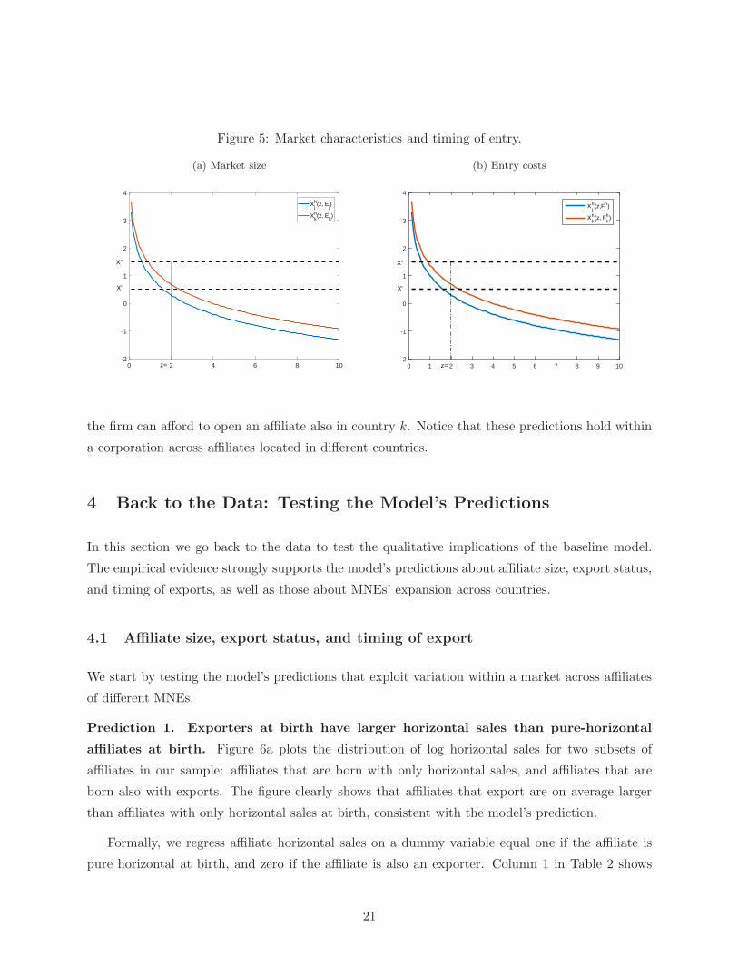
Figure 5: Market characteristics and timing of entry.
(a) Market size
0 2 4 6 8 10-2
-1
0
1
2
3
4
Xjh(z, E
j)
Xkh(z, E
k)
z=
X'
X''
(b) Entry costs
0 1 2 3 4 5 6 7 8 9 10-2
-1
0
1
2
3
4
Xjh(z,F
jh)
Xkh(z, F
kh)
z=
X'
X''
the firm can afford to open an affiliate also in country k. Notice that these predictions hold within
a corporation across affiliates located in different countries.
4 Back to the Data: Testing the Model’s Predictions
In this section we go back to the data to test the qualitative implications of the baseline model.
The empirical evidence strongly supports the model’s predictions about affiliate size, export status,
and timing of exports, as well as those about MNEs’ expansion across countries.
4.1 Affiliate size, export status, and timing of export
We start by testing the model’s predictions that exploit variation within a market across affiliates
of different MNEs.
Prediction 1. Exporters at birth have larger horizontal sales than pure-horizontal
affiliates at birth. Figure 6a plots the distribution of log horizontal sales for two subsets of
affiliates in our sample: affiliates that are born with only horizontal sales, and affiliates that are
born also with exports. The figure clearly shows that affiliates that export are on average larger
than affiliates with only horizontal sales at birth, consistent with the model’s prediction.
Formally, we regress affiliate horizontal sales on a dummy variable equal one if the affiliate is
pure horizontal at birth, and zero if the affiliate is also an exporter. Column 1 in Table 2 shows
21

Figure 6: Affiliate size, export status, and the timing of export entry.
(a) non-exporters vs exporters at birth
0.0
5.1
.15
.2.2
5.3
Den
sity
0 5 10 15log of affiliate’s horizontal sales
non−exporters at birth exporters at birth
kernel = epanechnikov, bandwidth = 0.2205
(b) early vs late exporters
0.1
.2.3
Den
sity
0 5 10 15log of affiliate’s horizontal sales
age of first export: 0−5 age of first export: 6−10
kernel = epanechnikov, bandwidth = 0.1968
Notes: Sample of new majority-owned affiliates that survive for at least ten consecutive years, in manufacturing. Kernel densityof log horizontal sales for affiliates that: are born with exclusively horizontal sales (non-exporters) and those with exports(exporters), in (6a); start exporting in their first five years of life and those that start after five years of life, in (6b).
that the negative correlation between size in the host market and being a pure horizontal affiliate
at birth survives the inclusion of an age control and of country-year and industry fixed effects.
Mimicking well-documented facts on domestic exporters, this result shows that affiliates that
export are larger in their host market than affiliates whose sales are limited to their host country.16
Prediction 2. Affiliates that start exporting earlier in life have larger horizontal sales
than late starters. Figure 6b illustrates the relationship between the size of an affiliate in its
host country, measured by the log of sales in the host country, and the time in the affiliate’s life
cycle at which it decides to export. We split the sample between affiliates that start exporting
in the first five years of life and affiliates that start exporting later in their life cycle. As the
figure shows, affiliates that start exporting earlier in life are larger in their host country compared
to affiliates that start exporting later. The pattern is robust to the choice of the age cutoff for
first exports (see Figure B.3 in Appendix B). Moreover, as column 2 in Table 2 shows, the negative
relationship between size in the host market and age at first export survives the inclusion of affiliate
age, country-year and industry fixed effects.
Column 3 in Table 2 combines Predictions 1 and 2 and shows that they jointly hold in the data.
16In a companion paper, Garetto et al. (2017) provide a thorough comparison of stylized facts about MNE exportersand non-MNE exporters.
22

Table 2: Affiliate size, by export status, timing of entry, and order in the affiliate opening sequence.OLS.
Dep var log of horizontal sales
(1) (2) (3) (4)
D(pure horizontal at birth) -0.979*** -0.698***(0.085) (0.079)
Age at first export -0.135*** -0.066***(0.015) (0.018)
D(first affiliate) 0.418***(0.111)
Age 0.069*** 0.072*** 0.065*** 0.080***(0.012) (0.018) (0.013) (0.010)
D(first affiliate)× Age -0.029***(0.010)
log global employment 0.421***(0.090)
Parent FE no no no yes
Obs 33,939 30,117 30,117 33,939R-sq 0.12 0.11 0.12 0.03
Note: Observations at the affiliate-year level, for new majority-owned affiliates that survive for at least ten consecutiveyears, in manufacturing. D(pure H at birth) is equal to one if the affiliate is born with only horizontal sales; andzero otherwise. D(1st affiliate) is equal to one if the affiliate is first in the opening sequence of the MNE; andzero otherwise. Global employment refers to the aggregate employment of the MNE, both in the United Statesand abroad. Pure exporters are excluded from the sample. All specifications include country-year and industryfixed effects. Standard errors, clustered at the parent level, are in parenthesis. Levels of significance are denoted∗∗∗p < 0.01, ∗∗p < 0.05, and ∗p < 0.1.
23

4.2 The expansion strategies of MNEs across countries
The second set of model’s predictions refer to the expansion of individual MNEs across different
host markets; that is, we exploit within-MNE variation across countries.
Prediction 3. MNEs open their largest affiliates first. Column 4 in Table 2 confirms this
prediction: horizontal sales are systematically larger for the first affiliate of a MNE, controlling for
affiliate age and size of the corporation. Notice that this specification includes country-industry
and parent fixed effects, so that we exploit variation across affiliates of the same MNE. Table B.4
in Appendix B provides more statistics differentiating first affiliates from subsequent ones: first
affiliates tend to have larger sales and employment than subsequent affiliates, and are more likely
to be exporters. Figure B.1 in Appendix B illustrates some of these size differences over the life
cycle.
Prediction 4. MNEs open affiliates first in larger markets. The model predicts sorting in
the order in which a MNE opens affiliates over time. The first row of Table B.4 illustrates that, on
average, affiliates located in a large host market open first.
Prediction 5. MNEs open affiliates first in markets with lower entry costs. Table 3
provides suggestive evidence supporting this prediction. As commonly done in the literature, we
proxy for entry costs using indicators from the World Bank’s Doing Business Database: the number
of administrative procedures required to open a business, the average number of days it takes to
open, the cost of starting a business as a percent of GDP per capita, and the minimum capital
requirement in US dollars. Table 3 makes clear that, under various measures, MNEs choose, on
average, to open affiliates first in markets that are less costly to enter. Countries in which MNEs
open their first affiliate have around a 20 percent lower number of business procedures, take 20,
rather than 25, days to open a business, and have a cost of starting a business that is two thirds of
the cost faced in subsequent markets. Additionally, on average, affiliates are first opened in markets
for which the minimum capital needed to start a business is 20 percent lower.
We conclude this section with some additional evidence in support of two of the model’s as-
sumptions: the independence assumption and the assumptions on the shock structure.
4.3 Extended gravity and the independence assumption
The tractability of the model hinges on the independence assumption, which postulates that both
the decisions of opening an affiliate and of exporting from it are independent across countries. We
find support for this assumption in the data.
24

Table 3: Affiliate size and market characteristics, by affiliate position in the MNE opening sequence.
Avg. first affiliates subsequent affiliates
GDP (billions of US$) 970 868
number of biz procedures 6.4 7.6
number of days to start biz 20.2 24.6
cost of start biz (% of GDPpc) 7.0 11.8
Min K needed to start biz (U$) 4,634 6,017
Note: Observations at the affiliate level, for new majority-owned affiliates that survive for at least ten consecutiveyears, in manufacturing. Variables related to entry costs are from the World Bank, Doing Business. GDP is fromthe Penn World Tables (8.0).
The independence assumption implies that it is possible for a firm to have an affiliate in a
country and at the same time to have affiliates elsewhere that export to that same country. This
is different from the models in Arkolakis et al. (2017) and Tintelnot (2017), in which each firm has
only one lowest-cost location to reach final consumers in a country.
Even though the BEA data contains limited information about the destination of affiliates’
exports, we are able to examine the coexistence of affiliates’ exports to three countries (Canada,
the United Kingdom, and Japan) with the presence of affiliates owned by the same parents in those
countries, for 2004.17 Our calculations imply that of the 20,359 affiliates that export to Canada, 64
percent belong to a U.S. parent that also has affiliates located in Canada. Similarly, of the 5,017
affiliates that export to the United Kingdom, 70 percent belong to a U.S. parent that also has
affiliates located in that country. Finally, of the 5,224 affiliates that export to Japan, 47 percent
belong to a U.S. parent that also has affiliates located in Japan.
A more direct test of the independence assumption is, for a given U.S. parent, the comparison
between the probability of owning an affiliate in a country and the same probability conditional
on already having an affiliate in a “neighboring” country (i.e. in a country belonging to the same
region). We follow Morales et al. (2015) and call the difference in these probabilities “extended
gravity”. Of course, the comparison is only possible for U.S. parents with at least two foreign
affiliates. Table B.5 in Appendix B shows the results for MNEs with at least two, five, and ten
affiliates worldwide, respectively. Countries are restricted to the ten most popular destinations for
U.S. MNEs that belong to four regions: North America, Europe, Latin America, and Asia (Central,
17Benchmark year surveys contain more information about affiliate export destinations than non-benchmark yearones.
25

South, and East Asia, plus the Pacific). Conditional and unconditional probabilities are strikingly
similar the larger the MNE in terms of number of affiliates worldwide. The largest differences are
observed when we include smaller MNEs (at least 2 affiliates) in countries –such as China– that are
typically part of global supply chains. Compared with the evidence for exporters in Morales et al.
(2015), extended gravity is much less pronounced for MNEs opening affiliates than for domestic
firms entering export destinations.
4.4 The structure of MNE shocks in the data
Our model assumes that the shock structure of MNEs is composed of a MNE-wide time-invariant
component and of a time-varying source-country component. Time-varying host-country compo-
nents also matter in industry equilibrium. How much of the variation in affiliates sales is captured
in the data by these shocks? Table B.6 in Appendix B illustrates that, while country-level time-
varying shocks and parent fixed effects explain almost a third of affiliate sales variation in the data,
parent-level time-varying variables (i.e. parent sales) contribute little to explain affiliate sales vari-
ation in the data. We interpret this evidence as support for our assumptions on the MNE shock
which does not rely in any time-varying firm-level component.
To conclude, the evidence in this section suggests that while in the cross-section, affiliates of
U.S. MNEs broadly behave like domestic exporters, in the time series, they display much flatter
growth profiles, more persistence, and less extended gravity than domestic exporters. The evidence
lends further support to modeling the cross-section of MNEs’ affiliates along the lines of a Melitz
model, and the time series with a productivity process that grows over time due to its aggregate
component, and not due to the idiosyncratic component.
5 Quantitative Analysis
We extend the model to make it amenable to quantitative analysis. To this end, firms can endoge-
nously decide to shut down affiliates, chose the destination of affiliate exports, and endogenously
decide to exit any export market. We close the model in industry equilibrium with aggregation
and determination of the country-level price indexes.
Incorporating endogenous exit is important for two reasons. Empirically, exit rates decline with
affiliate age and size, but are independent of whether the affiliate is an exporter or not (see Table
B.7 in Appendix B). Quantitatively, incorporating endogenous exit rates in the model allows to
separately identify the sunk and fixed costs of affiliate opening by matching moments on entry and
26
exit rates, respectively. In turn, incorporating the choice of the destination of exports for affiliates
will allow us to separately identify costs related to the Home market and to third markets, and
possibly to separate vertical investment motives distinguishing sales back to the U.S. market.
5.1 Quantitative model
Extending the model to endogenous exit, from a host country and from export markets, is straight-
forward. The value functions include an extra term, which is the option value of exit, as well as
additional value-matching and smooth pasting conditions that deliver the exit thresholds.
Modeling the choice of the destination of affiliate exports is more complex. An affiliate located
in any country j can in principle export to any subset of the set of potential export destinations,
and the value of an exporting affiliate depends on the set of countries in which the affiliate exports.
To maintain the problem tractable, we resort again to an independence assumption. Precisely,
we assume that the decision of an affiliate located in country j to export to a country k 6= j is
independent from the decision to export to any other country. Relying on this assumption, we
can write the problem of the firm as a compound option and solve it backwards, as suggested by
Dixit and Pindyck (1994, chap. 10). In other words, conditional on the firm having an affiliate in
country j, we solve for the value of exports and of horizontal sales, and determine the thresholds
that induce the affiliate to export or stop exporting to each country k 6= j. Once determined the
value of an affiliate in country j, we solve for the thresholds that induce the firm to open or shut
down that affiliate.
The value of a firm with productivity z when the state of the economy is X is:
V(z,X) = Vd(z,X) +
N∑
j=1
max
V oj (z,X), V a
j (z,X)
, (25)
where Vd(z,X) is the value of domestic sales, V oj (z,X) is the option value of opening an affiliate
in country j, and V aj (z,X) is the value of an affiliate in country j, regardless of the destination of
its sales. In turn, we can define V aj (z,X) as
V aj (z,X) = V h
j (z,X) +∑
k 6=j
max
V ojk(z,X), V e
jk(z,X)
, (26)
where V hj (z,X) is the value of horizontal sales, V o
jk(z,X) is the option value of exporting to country
k for an affiliate located in j, and V ejk(z,X) is the value of exports to country k for an affiliate
located in j. This formulation of the problem is analogous to a compound option because opening
27

an affiliate in a country is equivalent to exercising an option that gives access to another set of
options: the options to export to any other country.
We start by solving for V ojk(z,X) and V e
jk(z,X), conditional on the firm having an affiliate in
country j. This is a simple case of interlinked options (see Dixit and Pindyck 1994, chap. 7), that
gives as solution:
V ojk(z,X) = Bo
jk(z)eβX (27)
V ejk(z,X) =
πejk(z,X)
ρ+ δ − µ−
f ejk
ρ+ δ+Ae
jk(z)eαX (28)
where Bojk(z) > 0 and Ae
jk(z) > 0 are firm-specific parameters, and α < 0, β > 1 are the roots of12σ
2β2 + µβ − (ρ + δ) = 0. As Bojk(z)e
βX represents the option value of exporting to country k,
and is increasing in the realization of the aggregate productivity shock, similarly Aejk(z)e
αX is the
option value of quitting the export market k, and is decreasing in the realization of the aggregate
productivity shock, indicating that the option of exiting an export market has a larger value in
“bad times”.
For each country pair (j, k) and for each firm with productivity z, the parameters Bojk(z) > 0,
Aejk(z) > 0, and the aggregate productivity thresholds that induce the affiliate to start and stop
exporting, denoted by XOEjk and XEO
jk , respectively, can be recovered from the following system of
value-matching and smooth pasting conditions,
V ojk(z,X
OEjk ) = V e
jk(z,XOEjk )− F e
jk (29)
V ojk(z,X
EOjk ) = V e
jk(z,XEOjk ) (30)
V ′ojk(z,X
OEjk ) = V ′e
jk(z,XOEjk ) (31)
V ′ojk(z,X
EOjk ) = V ′e
jk(z,XEOjk ). (32)
The value of horizontal sales, conditional on having an affiliate, is given by the present discounted
value of profits from horizontal sales plus the option value of shutting down the affiliate,
V hj (z,X) =
πhj (z,X)
ρ+ δ − µ−
fhj
ρ+ δ+Ah
j (z)eαX , (33)
where Ahj (z) > 0 is a firm-specific parameter.
28

The value of an affiliate in country j can then be written as
V aj (z,X) =
πhj (z,X)
ρ+ δ − µ−
fhj
ρ+ δ+Ah
j (z)eαX+
∑
k∈Aj(z)
[
πejk(z,X)
ρ+ δ − µ−
f ejk
ρ+ δ+Ae
jk(z)eαX
]
+∑
k 6∈Aj(z)
[
Bojk(z)e
βX]
(34)
whereAj(z) denotes the set of export markets to which the affiliate in j with productivity z exports.
The independence assumption is clearly shown in (34): the value of an affiliate does not depend on
the sales or on the value of the firm’s other affiliates in other countries, but it does depend on the
set of potential export destinations from the affiliate’s host country.
It remains to solve for the decision of a firm to set up an affiliate in country j. The option value
of opening an affiliate in j is
V oj (z,X) = Bo
j (z)eβX . (35)
Hence, for each host country j and for each firm with productivity z, the parameters Boj (z) > 0,
Ahj (z) > 0, and the aggregate productivity thresholds that induce the firm to open and shut down
an affiliate, denoted by XOHj , XHO
j , respectively, can be recovered from the following system of
value-matching and smooth pasting conditions,
V oj (z,X
OHj ) = V a
j (z,XOHj )− F h
j (36)
V oj (z,X
HOj ) = V a
j (z,XHOj ) (37)
V ′oj(z,X
OHj ) = V ′a
j (z,XOHj ) (38)
V ′oj(z,X
HOj ) = V ′a
j (z,XHOj ). (39)
Lastly, the value of domestic sales is simply given by the present discounted value of profits
from domestic sales,
Vd(z,X) =πd(z,X)
ρ+ δ − µ. (40)
Details about the solution of the model are contained in Appendix C.
5.2 Industry equilibrium
The industry equilibrium in this economy is defined by a vector of price indexes Pk, for k = 1, ...N ,
and by laws of motion ruling the evolution of affiliate operations over time across countries. The
29
price index in country k at time k is
P 1−ηk =
N∑
i=1
N∑
j=1
P 1−ηijk (41)
where Pjk(t) denotes the price index of varieties produced by affiliates of Home firms located in
country j and selling to country k, at time t,
P 1−ηjk (t) =
∫
Ωjk
(τjkwj
zZ
)1−η
dz, (42)
where Ωjk is the set of Home firms having affiliates in j that export to k.
Let Mi denote the (exogenous) mass of firms from country i. The endogenous mass of affiliates
of firms from i located in j, Mij , is given by continuing affiliates plus new affiliates,
M ′ij = Mij · (1−Gi(z
HOij )) + (Mi −Mij) · (1−Gi(z
OHij )), (43)
while the mass of affiliates of firms from i located in j that export to k is given by continuing
exporting affiliates to k plus new exporters to k,
M ′ijk = Mijk · (1−Gi(z
EOijk )) + (Mij −Mijk) · (1−Gi(z
OEijk )). (44)
The variable zOHij (zHO
ij ) is the productivity threshold that induces a firm from i to open (shut
down) an affiliate in j, while zOEijk (zEO
ijk ) is the productivity threshold that induces an affiliate of
a firm from i in j to start (stop) exporting from j to k.18 Finally, Gi(z) denotes the c.d.f. of the
(exogenous) firm-level productivity distribution in country i.
5.3 Numerical example: the rise of China
We illustrate the mechanisms of the quantitative model with a numerical example. Assume that
there are three countries: the United States, Japan, and China. As in our data, multinational
firms are headquartered in the United States. They have to decide whether and where to open
affiliates and whether the affiliates will sell only to the host market or also export. The purpose
of this numerical exercise is to show that different changes in the cost structure of multinational
activity across host countries generate differences in the number of affiliates, sales, and the share
of affiliates that exports, by age.
18Theorem 1 in Fillat and Garetto (2015) assures that these firm-level productivity thresholds are well-defined.
30

We start with a scenario where China is identical to Japan. In this case, we set w = P = Q = 1,
F h = 10, F e = 8, τ = 2, and f e = fh = 0.3. A more realistic scenario is one where China is poorer,
but larger, than Japan. In this case we set wchn = Pchn = 0.6 and Qchn = 2; we will refer to this
as our “baseline” scenario.
Keeping the baseline values for wages and expenditure unchanged, we perform three comparative
statics exercises, meant to depict the “rise of China” in the different ways that our model allows:
a drop in iceberg trade costs from China to Japan; a drop in the sunk cost of entering China; and
a drop in the sunk cost of exporting from China to Japan. To explore the effect of a reduction in
the affiliate entry cost, we lower the fixed cost F hchn such that the per-period cost of horizontal FDI
(fhchn+ (ρ+ δ)F h
chn) drops by ten percent. Similarly, to explore the differential effects of reductions
in iceberg versus fixed costs of exports, we lower either τchn,jpn or F echn,jpn in such a way that the
per-period cost of affiliate exports ((f echn + (ρ+ δ)F e
chn)τchn,jpn) drops by ten percent. Notice that
in this way, a static model would generate exactly the same comparative statics following a change
in Fe and a change in τ , so that this exercise is well suited to illustrate the different predictions of
our model compared to static ones.19
Table 4 reports the number of U.S. affiliates located in China and Japan, respectively, under
each scenario. Of course, in the symmetric case, the United States opens the same number of
plants in the two host countries. As expected, in the baseline scenario where China is larger and
poorer than Japan, the number of affiliates located in China increases. Starting from the baseline
scenario, a decrease in the sunk cost of opening an affiliate increases the numbers of affiliates located
in China. However, changes in the costs of affiliate exports from China to Japan do not change
the number of U.S. affiliates that choose to operate in China and survive at least than ten periods.
The fact that the number of U.S. affiliates located in Japan does not change with shocks to China’s
MNE costs is just a consequence of our independence assumption on the MNE location choices and
of the partial equilibrium nature of this example.
Figure 7 shows the share of exporting affiliates located in Japan (left panel) and China (right
panel) in each of the described scenarios, by age. As expected, in the symmetric case those shares
are the same. In the baseline case, where China is larger and poorer, more U.S. firms open affiliates
in China than in Japan, and those affiliates have lower costs than the ones in Japan, so that they
are more likely to export. Notice that quantitatively, the cost savings of U.S. affiliates in China
dominate the fact that U.S. affiliates located in Japan have a larger export market.
19The remaining parameters of the model are: the time preference parameter, ρ = 0.02; the exogenous deathrate, δ = 0.01; the elasticity of substitution, η = 2; the drift for the productivity process, µ = 0.02; the standarddeviation for the productivity process σ = 0.06; the Pareto-shape parameter, θ = 3; and the lower bound of thePareto distribution, b = 1. We simulate 500 affiliates and 50 periods.
31

Table 4: Number of U.S. affiliates abroad, by country. Three-country simulation.
symmetry baseline low τchn,jpn low F echn,jpn low F h
chn
Japan 191 191 191 191 191
China 191 352 352 352 403
Notes: Affiliates that survive at least ten periods in the model, in each country.
Figure 7: Share of exporters, by age. Three-country simulation
1 2 3 4 5 6 7 8 9 100
0.01
0.02
0.03
0.04
0.05
0.06
0.07
0.08
0.09
0.1
Age
shar
e o
f U
.S. a
ffili
ates
th
at e
xpo
rt
Japan
China = JapanChina poorer but largerChina low tauChina low FhChina low Fe
1 2 3 4 5 6 7 8 9 100
0.1
0.2
0.3
0.4
0.5
0.6
0.7
0.8
0.9
1China
Age
shar
e o
f U
.S. a
ffili
ates
th
at e
xpo
rt
The decrease in the sunk cost Fh significantly increases the number of affiliates in China, but not
their likelihood to export, which actually decreases as less productive affiliates enter. In contrast,
changes in the variable and the sunk cost of affiliate exports do not affect the number of affiliates,
but increase their probability to export. It is interesting how the reduction in the sunk cost of
export generates a larger effect than the reduction in the variable cost, despite the numbers being
chosen so that the change in per-period costs is the same. The reason for this difference is that
when Fe decreases, not only the per period cost decreases, but also the band of inaction shrinks.
In other words, affiliates are more likely to start exporting because now their optimal choices are
more flexible. The overall effect of Fe is larger than the one of τ because it is a combination of a
static and a dynamic effect.
Finally, Figure 8 shows average horizontal sales and total sales of affiliates located in Japan
32

Figure 8: Affilate sales, by age. Three-country simulation.
1 2 3 4 5 6 7 8 9 101
1.1
1.2
1.3
1.4
1.5
1.6
1.7
1.8
Age
To
tal s
ales
, rel
to
ag
e 1
Japan, all sales
China = JapanChina poorer but largerChina low tauChina low FhChina low Fe
1 2 3 4 5 6 7 8 9 101
1.1
1.2
1.3
1.4
1.5
1.6
1.7
1.8China, all sales
Age
To
tal s
ales
, rel
to
ag
e 1
1 2 3 4 5 6 7 8 9 101
1.1
1.2
1.3
1.4
1.5Japan, horizontal sales
Age
Ho
rizo
nta
l sal
es, r
el t
o a
ge
1
1 2 3 4 5 6 7 8 9 101
1.1
1.2
1.3
1.4
1.5China, horizontal sales
Age
Ho
rizo
nta
l sal
es, r
el t
o a
ge
1
Notes: Affiliates that survive at least ten periods in the model. Averages across affiliates.
(left panel) and China (right panel) in each of the described scenarios. The “rise of China” has
interesting effects on the affiliates’ sales in the countries were the affiliates locate and export to.
As the variable cost τchn,jpn declines, Chinese affiliates become more profitable because exporting
is now less costly. This decline induces more entry in China and increases exports to Japan. Lower
entry costs into China barely have an effect on horizontal and total sales of Chinese affiliates, while
lower sunk costs of exports for Chinese affiliates have the effect of increasing total sales of Chinese
affiliates via exports.
5.4 Calibration
[TO BE COMPLETED]
6 Conclusions
This paper is a theoretical and empirical investigation of how the activities of multinational corpo-
rations evolve over the life cycle. We establish three novel facts: first, MNEs’ affiliates grow little
33

over their life cycle; second, MNEs affiliates’ are born specialized in their life-long activity; and
third, they diversify a small share of their activities over their life cycle.
These facts guide us in the construction of a simple dynamic model of multinational activity
which, albeit stylized, delivers rich testable implications for which we find strong support in the
data.
The quantitative model sheds light on the implications of dynamic features of the data for the
magnitudes and characteristics of the costs to the MNE, an essential ingredient to study the welfare
gains from multinational activity.
References
Alessandria, G. and H. Choi (2007). Do sunk costs of exporting matter for net exports dynamics?
Quarterly Journal of Economics 122 (1), 289–336.
Alessandria, G., H. Choi, and K. Ruhl (2015). Trade adjustment dynamics and the welfare gains
from trade. Mimeo, University of Rochester.
Antras, P. and S. R. Yeaple (2014). Multinational firms and the structure of international trade.
Handbook of International Economics 4, 55–130.
Arkolakis, C. (2016). A unified theory of firm selection and growth. Quarterly Journal of Eco-
nomics 131 (1), 89–155.
Arkolakis, C., N. Ramondo, A. Rodrıguez-Clare, and S. Yeaple (2017). Innovation and production
in the global economy. NBER WP 18792.
Baldwin, R. and P. Krugman (1989). Persistent trade effects of large exchange rate shocks. Quar-
terly Journal of Economics 104 (4), 635–654.
Bernard, A. B. and J. B. Jensen (1999). Exceptional exporter performance: cause, effect, or both?
Journal of International Economics 47, 1–25.
Conconi, P., A. Sapir, and M. Zanardi (2016). The internationalization process of firms: from
exports to fdi. Journal of International Economics 99, 16–30.
Cravino, J. and A. Levchenko (2017). Multinational firms and international business cycle trans-
mission. Quarterly Journal of Economics, Forthcoming 132 (2), 921–962.
34
Das, S., M. J. Roberts, and J. R. Tybout (2007). Market entry costs, producer heterogeneity, and
export dynamics. Econometrica 75 (3), 837–873.
Davis, S. J., J. Haltiwanger, and S. Schuh (1996). Small business and job creation: Dissecting the
myth and reassessing the facts. Small Business Economics 8 (4), 297–315.
Decker, R., J. Haltiwanger, R. Jarmin, and J. Miranda (2014). The role of entrepreneurship in us
job creation and economic dynamism. Journal of Economic Perspectives 28 (3), 3–24.
Decker, R., J. Haltiwanger, R. Jarmin, and J. Miranda (2015). Where has all the skewness gone?
the decline in high-growth (young) firms in the u.s. NBER Working Paper # 21776.
Dixit, A. K. and R. S. Pindyck (1994). Investment under Uncertainty. Princeton, NJ: Princeton
University Press.
Eaton, J., M. Eslava, M. Kugler, and J. Tybout (2008). The margins of entry into export markets:
Evidence from colombia. In E. Helpman, D. Marin, and T. Verdier (eds.), The Organization of
Firms in a Global Economy. Cambridge, MA: Harvard University Press.
Egger, P., M. Fahn, V. Merlo, and G. Wamser (2014). On the genesis of multinational foreign
affiliate networks. European Economic Review 65, 136–163.
Fillat, J. L. and S. Garetto (2015). Risk, returns, and multinational production. Quarterly Journal
of Economics 130 (4), 2027–2073.
Fillat, J. L., S. Garetto, and L. Oldenski (2015). Diversification, cost structure, and the risk
premium of multinational corporations. Journal of International Economics 96 (1), 37–54.
Garetto, S., L. Oldenski, N. Pandalai-Nayar, and N. Ramondo (2017). Exporters. Mimeo.
Ghironi, F. and M. J. Melitz (2005). International trade and macroeconomic dynamics with het-
erogeneous firms. The Quarterly Journal of Economics 120 (3), 865–915.
Gravelle, J. (2015). Tax havens: International tax avoidance and evasion. Congressional Research
Service 7 (5700), 1–55.
Gumpert, A., A. Moxnes, N. Ramondo, and F. Tintelnot (2016). Multinational firms and exporters
dynamics. Mimeo, UCSD.
Helpman, E., M. J. Melitz, and S. R. Yeaple (2004). Exports versus fdi with heterogeneous firms.
American Economic Review 94 (1), 300–316.
35
Impullitti, G., A. A. Irarrazabal, and L. D. Opromolla (2013). A theory of entry and exit into
exports markets. Journal of International Economics 90 (1), 75–90.
Kueng, L., M.-J. Yang, and B. Hong (2016). Sources of firm life-cycle dynamics: Size vs. age effects.
Mimeo, University of Washington.
Melitz, M. J. (2003). The impact of trade on intra-industry reallocations and aggregate industry
productivity. Econometrica 71 (6), 1695–1725.
Morales, E., G. Sheu, and A. Zahler (2015). Extended gravity. Mimeo, Princeton University.
Ramondo, N., V. Rappoport, and K. J. Ruhl (2013). The proximity-concentration tradeoff under
uncertainty. Review of Economic Studies 80 (4), 1582–1621.
Roberts, M. J. and J. R. Tybout (1997). The decision to export in colombia: An empirical model
of entry with sunk costs. The American Economic Review 87 (4), 545–564.
Ruhl, K. J. and J. Willis (2017). New exporter dynamics. International Economics Review 58 (3).
Tintelnot, F. (2017). Global production with export platforms. Quarterly Journal of Eco-
nomics 132 (1), 157–209.
Appendix
A Data Description and Summary Statistics
To describe the construction of our sample, it is important to notice that the BEA surveys affiliates
of U.S. parents applying minimum survey exemption levels, in terms of affiliate sales, which differ
over time. In general, reporting thresholds increased in recent years, reaching US$60 millions for
2011. Additionally, benchmark survey years (i.e., years in which the survey is more comprehen-
sive), which occur every 4 years, have lower reporting thresholds. Table A.1 shows the reporting
thresholds for the years in our sample.
Since the goal of this paper is to understand the evolution of the global structure of production,
and not the establishment of headquarters due to profit shifting motives, we restrict our attention
to affiliates that do not operate in tax haven countries. Affiliates in tax haven countries are likely
to open for different reasons and be subject to different cost structures than those in non-tax haven
countries, confounding our analysis. We compile our list of tax havens using information from
36

Table A.1: BEA minimum survey exemptions levels
survey year Minimum exemption levels survey year Minimum exemption levels(in U$ millions) (in U$ millions)
1987-88 10 2000-03 301989 3 2004 25
1990 -93 15 2005-07 401994 3 2008 601995-98 20 2009 25
1999 7 2010-11 60
Note: Exemption levels are for majority-owned foreign affiliates. Benchmark survey years are highlighted.
Gravelle (2015). We omit countries that meet some of the criteria for tax haven status but that
also have a substantial amount of real FDI production from the list. If a country is in the top ten
percent of U.S. FDI destinations measured by total U.S. MNE affiliate employment, we consider
it to be a location for actual production rather than a strict tax haven. Based on this definition,
Ireland, Switzerland, Hong Kong, and Singapore are the only countries from the Gravelle (2015)
list that we do not classify as tax havens. A full list of tax haven countries is reported below (TBA).
When a firm has more than one enterprise operating in the same country and industry, we
group these enterprises’ activities together and refer to them as a single affiliate. We do this for
two reasons. First, the firms themselves are permitted to report combined data in this way, making
it difficult to isolate individual plants. Based on the BEA definition, an affiliate is a business
enterprise in a given industry operating in a particular host country; it thus could operate several
plants in different locations within the host country. The BEA rules permit consolidated reporting
for distinct enterprises located in the same country that operate in the same narrowly defined
industry or otherwise are integral parts of the same business operation. Second, to the extent that
the costs of opening a new affiliate are incurred at the country-industry level, this is the appropriate
level of aggregation for our analysis. In a robustness exercise, we use reported openings of new
enterprises in a country-industry in which the firm already had existing affiliates to check whether
costs are incurred at the enterprise or country-industry level. This exercise, though based on noisy
data, confirms that focusing on the country-industry-firm-, rather than plant-level, is appropriate.
Table A.2 shows in more detail the distribution of horizontal sales and exports as a share of
total affiliate sales. On average, around 72 percent of the sales of an affiliate are destined to the host
market, while the remaining 28 percent are exports. The distribution of export sales is extremely
skewed: while the 25th percentile of the horizontal shares distribution is above 50 percent and
37
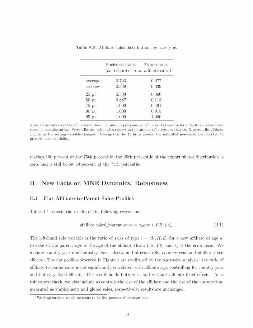
Table A.2: Affiliate sales distribution, by sale type.
Horizontal sales Export sales(as a share of total affiliate sales)
average 0.723 0.277std dev 0.339 0.339
25 pc 0.539 0.00050 pc 0.887 0.11375 pc 1.000 0.46190 pc 1.000 0.91595 pc 1.000 1.000
Note: Observations at the affiliate-year level, for new majority-owned affiliates that survive for at least ten consecutiveyears, in manufacturing. Percentiles are taken with respect to the variable of interest so that the X-percentile affiliateschange as the sorting variable changes. Averages of the 11 firms around the indicated percentile are reported topreserve confidentiality.
reaches 100 percent at the 75th percentile, the 25th percentile of the export shares distribution is
zero, and is still below 50 percent at the 75th percentile.
B New Facts on MNE Dynamics: Robustness
B.1 Flat Affiliate-to-Parent Sales Profiles
Table B.1 reports the results of the following regression:
affiliate salesia/parent sales = βaage+ FE + εia. (B.1)
The left-hand side variable is the ratio of sales of type i = all,H,E, for a new affiliate of age a,
to sales of the parent, age is the age of the affiliate (from 1 to 10), and εia is the error term. We
include country-year and industry fixed effects, and alternatively, country-year and affiliate fixed
effects.1 The flat profiles observed in Figure 1 are confirmed by the regression analysis: the ratio of
affiliate to parent sales is not significantly correlated with affiliate age, controlling for country-year
and industry fixed effects. The result holds both with and without affiliate fixed effects. As a
robustness check, we also include as controls the size of the affiliate and the size of the corporation,
measured as employment and global sales, respectively; results are unchanged.
1We drop outliers which turn out to be five percent of observations.
38

Table B.1: Affiliate-to-parent sales ratio, by sales type. OLS.
Dep var affiliate-to-parent sales ratio
all sales horizontal sales export sales
(1) (2) (3) (4) (5) (6)affiliate age 0.019 0.005 0.011 0.002 0.011 0.004*
(0.014) (0.003) (0.007) (0.001) (0.012) (0.002)
industry fe yes no yes no yes nocountry-year fe yes yes yes yes yes yesaffiliate fe no yes no yes no yes
Observations 38,088 38,088 36,127 36,127 25,950 25,950R-square 0.01 0.0002 0.04 0.0003 0.01 0.0001
Note: Observations at the affiliate-year level, for new majority-owned affiliates that survive for at least ten consecutive years, inmanufacturing. The dependent variable affiliate to parent sales refers to affiliate sales in each type, relative to the domesticsales of the U.S. parent. Standard errors, clustered at the parent level, are in parenthesis. Levels of significance are denoted∗∗∗p < 0.01, ∗∗p < 0.05, and ∗p < 0.1.
As a further step to describe sales growth profiles of different affiliates, Figure B.1 shows that
first affiliates are much larger than subsequent affiliates, but they do not appear to grow faster.
Figure B.1: Affiliate size, by activity type, age, and position in the MNE opening sequence.
(a) total sales
0.0
5.1
.15
.2.2
5af
filia
te s
ales
rel
ativ
e to
par
ent U
S s
ales
1 2 3 4 5 6 7 8 9 10Affiliate age
First affiliates Subsequent affiliates
(b) horizontal sales
0.0
5.1
.15
.2.2
5af
filia
te s
ales
rel
ativ
e to
par
ent U
S s
ales
1 2 3 4 5 6 7 8 9 10Affiliate age
First affiliates Subsequent affiliates
(c) export sales
0.0
5.1
.15
.2.2
5
affil
iate
sal
es r
elat
ive
to p
aren
t US
sal
es
1 2 3 4 5 6 7 8 9 10Affiliate age
First affiliates Subsequent affiliates
Notes: Sample of new majority-owned affiliates that survive for at least ten consecutive years, in manufacturing. First affiliatesrefer to the first affiliates opened by the MNE, while subsequence affiliates refer to the rest (2nd, 3rd, ..., nth).
39

Table B.2: Intensive and extensive margins of sale shares. OLS.
Dep var Intensive margin of sale shares Extensive margin of sale shares
horizontal sales export sales horizontal sales export sale share
(1) (2) (3) (4) (5) (6) (7) (8)
affiliate age -0.002 -0.012*** -0.005** 0.005*** 0.00003 -0.001 0.014*** 0.029(0.002) (0.001) (0.002) (0.001) (0.001) (0.0006) (0.003) (0.002)
industry fe yes no yes no yes no yes nocountry-year fe yes yes yes yes yes yes yes yesaffiliate fe no yes no yes no yes no yes
Observations 36,127 36,127 25,950 25,950 38,088 38,088 38,088 38,088R-square 0.079 0.013 0.092 0.000 0.042 0.0001 0.081 0.036
Note: Observations at the affiliate-year level, for new majority-owned affiliates that survive for at least ten consecutive years,in manufacturing. In columns (1)-(4), the dependent variable is horizontal (export) sales, as a share of total affiliate’s sales, foraffiliates with positive horizontal (export) sales; in columns (5)-(8), the dependent variable is the share of affiliates with positivehorizontal (export) sales. Standard errors, clustered at the parent level, are in parenthesis. Levels of significance are denoted∗∗∗p < 0.01, ∗∗p < 0.05, and ∗p < 0.1.
B.2 Affiliate Expansion over Time
To illustrate the evolution of horizontal and export sales shares over time, Table B.2 reports the
results of the following regression:
affiliate salesia/total affiliate salesa = βaage+ FE + εia (B.2)
where the left-hand side variable is the share of horizontal (export) sales of the affiliate, age is the
age of the affiliate (from 1 to 10), and εia is an error term. We include country-year and industry
fixed effects, and alternately, country-year and affiliate fixed effects.
Table B.2 shows the results. The regressions confirm that – within affiliates – the horizontal sales
share decreases and the export sales share increase, supporting the idea of increasing diversification
of affiliate sales in space over time. On the extensive margin, the share of affiliates selling to their
host market does not change over the life cycle, while the share of exporters increases, confirming
that affiliates add sales destinations over time.
Figure B.2 shows the evolution of the intensive and extensive margins of sales shares for affiliates
that are pure-type at birth. It is worth remembering that around 50 percent of affiliates are born
with only horizontal sales, while affiliates born with only exports are less than five percent of
40
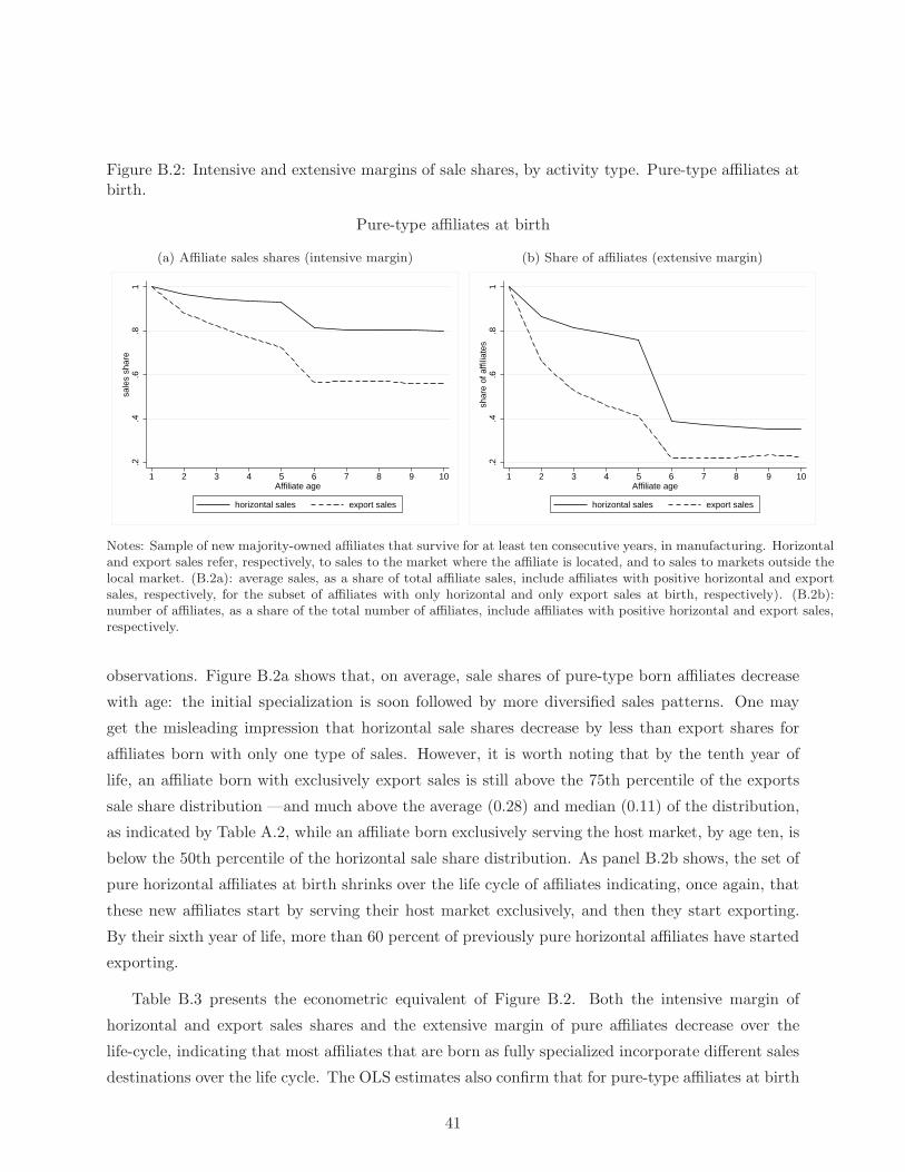
Figure B.2: Intensive and extensive margins of sale shares, by activity type. Pure-type affiliates atbirth.
Pure-type affiliates at birth
(a) Affiliate sales shares (intensive margin)
.2.4
.6.8
1sa
les
shar
e
1 2 3 4 5 6 7 8 9 10Affiliate age
horizontal sales export sales
(b) Share of affiliates (extensive margin)
.2.4
.6.8
1sh
are
of a
ffilia
tes
1 2 3 4 5 6 7 8 9 10Affiliate age
horizontal sales export sales
Notes: Sample of new majority-owned affiliates that survive for at least ten consecutive years, in manufacturing. Horizontaland export sales refer, respectively, to sales to the market where the affiliate is located, and to sales to markets outside thelocal market. (B.2a): average sales, as a share of total affiliate sales, include affiliates with positive horizontal and exportsales, respectively, for the subset of affiliates with only horizontal and only export sales at birth, respectively). (B.2b):number of affiliates, as a share of the total number of affiliates, include affiliates with positive horizontal and export sales,respectively.
observations. Figure B.2a shows that, on average, sale shares of pure-type born affiliates decrease
with age: the initial specialization is soon followed by more diversified sales patterns. One may
get the misleading impression that horizontal sale shares decrease by less than export shares for
affiliates born with only one type of sales. However, it is worth noting that by the tenth year of
life, an affiliate born with exclusively export sales is still above the 75th percentile of the exports
sale share distribution —and much above the average (0.28) and median (0.11) of the distribution,
as indicated by Table A.2, while an affiliate born exclusively serving the host market, by age ten, is
below the 50th percentile of the horizontal sale share distribution. As panel B.2b shows, the set of
pure horizontal affiliates at birth shrinks over the life cycle of affiliates indicating, once again, that
these new affiliates start by serving their host market exclusively, and then they start exporting.
By their sixth year of life, more than 60 percent of previously pure horizontal affiliates have started
exporting.
Table B.3 presents the econometric equivalent of Figure B.2. Both the intensive margin of
horizontal and export sales shares and the extensive margin of pure affiliates decrease over the
life-cycle, indicating that most affiliates that are born as fully specialized incorporate different sales
destinations over the life cycle. The OLS estimates also confirm that for pure-type affiliates at birth
41

Table B.3: Intensive and extensive margins of sale shares, pure-type affiliates at birth. OLS.
Dep var Intensive margin of sale shares Extensive margin of sale shares
horizontal sales export sales horizontal sales export sale share
(1) (2) (3) (4) (5) (6) (7) (8)
affiliate age -0.014*** -0.096*** -0.036** -0.021*** -0.046*** -0.044*** -0.059*** -0.038***(0.001) (0.001) (0.004) (0.003) (0.004) (0.002) (0.005) (0.004)
industry fe yes no yes no yes no yes nocountry-year fe yes yes yes yes yes yes yes yesaffiliate fe no yes no yes no yes no yes
Observations 19,463 19,463 3,032 3,032 19,905 19,905 3,595 3,595R-square 0.147 0.020 0.288 0.133 0.245 0.099 0.268 0.125
Note: Observations at the affiliate-year level, for new majority-owned affiliates that survive for at least ten consecutive years,in manufacturing. In columns (1)-(4), the dependent variable is horizontal (export) sales, as a share of total affiliate’s sales,for affiliates born with only horizontal (export) sales; in columns (5)-(8), the dependent variable is the share of affiliates bornwith only horizontal (export) sales. Standard errors, clustered at the parent level, are in parenthesis. Levels of significance aredenoted ∗∗∗p < 0.01, ∗∗p < 0.05, and ∗p < 0.1.
the decrease in sales shares is a result of within-affiliate changes: on average, affiliates of different
ages have undistinguishable export shares, but a pure exporter at birth decreases its export shares
as it gets older; for pure horizontal affiliates at birth, the effect is a mix of between- and within-firm
effects.
B.3 Testing the Predictions of the Model
Figure B.3 illustrates the relationship between affiliate size and timing of export for different time
cutoffs.
Table B.4 illustrates systematic differences between the first affiliate and subsequent affiliates
of a MNE in terms of size (defined as sales and employment) and likelihood of being an exporter.
Table B.5 provides support for the independence assumption by comparing the unconditional
probability that a MNE opens an affiliate in a country with the probability of opening conditional on
already having an affiliate in a “neighboring” country (i.e., a country located in the same continent.
Finally, table B.6 provides support for the structure of shocks that we assumed in the model by
illustrating that aggregate country-specific shocks and parent fixed effects account about 30 percent
of the variation in affiliate sales in our sample.
42

Table B.4: Affiliate size, by affiliate position in the MNE opening sequence.
Avg. first affiliates subsequent affiliates
affiliate employment 709 526
affiliate sales, as % of parent’s 20 6.5
affiliate H-sales, as % of parent’s 10 3.8
diversified affiliates (%) 65.7 59.3
Note: Observations at the affiliate level, for new majority-owned affiliates that survive for at least 10 consecutiveyears, in manufacturing.
Table B.5: Probabilities of observing affiliates in top-ten most popular destinations.
Probability of observing an affiliate in the same regionMNEs with: at least 10 affiliates at least 5 affiliates at least 2 affiliates
unconditional conditional unconditional conditional unconditional conditional
1 Canada 0.61 0.70 0.51 0.62 0.42 0.542 United Kingdom 0.68 0.64 0.62 0.64 0.57 0.593 Germany 0.71 0.72 0.60 0.62 0.40 0.514 Ireland 0.30 0.30 0.21 0.22 0.13 0.165 China 0.66 0.68 0.48 0.54 0.29 0.446 France 0.70 0.71 0.57 0.59 0.36 0.457 Brazil 0.60 0.60 0.50 0.47 0.26 0.318 Singapore 0.45 0.46 0.46 0.36 0.19 0.289 Mexico 0.61 0.70 0.50 0.54 0.32 0.4010 Japan 0.31 0.32 0.25 0.22 0.21 0.21
Note: Countries in the list belong to four regions (Europe, Asia, Latin America, and North America). Conditionalprobabilities refer to the probability of observing an affiliate country i given that the parent has an affiliate in a differentcountry of the same region. The number of parents with at least X affiliates worldwide is: 2,896 (X=10), 6,562 (X=5), and14,974 (X=2).
43
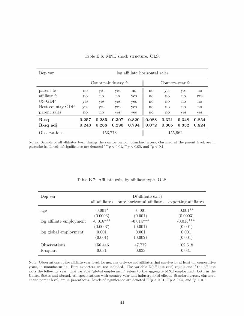
Table B.6: MNE shock structure. OLS.
Dep var log affiliate horizontal sales
Country-industry fe Country-year fe
parent fe no yes yes no no yes yes noaffiliate fe no no no yes no no no yesUS GDP yes yes yes yes no no no noHost country GDP yes yes yes yes no no no noparent sales no no yes yes no no yes yes
R-sq 0.257 0.285 0.307 0.829 0.088 0.321 0.348 0.854
R-sq adj 0.243 0.268 0.290 0.794 0.072 0.305 0.332 0.824
Observations 153,773 155,962
Notes: Sample of all affiliates born during the sample period. Standard errors, clustered at the parent level, are inparenthesis. Levels of significance are denoted ∗∗∗p < 0.01, ∗∗p < 0.05, and ∗p < 0.1.
Table B.7: Affiliate exit, by affiliate type. OLS.
Dep var D(affiliate exit)all affiliates pure horizontal affiliates exporting affiliates
age -0.001* -0.001 -0.001**(0.0003) (0.001) (0.0003)
log affiliate employment -0.016*** -0.014*** -0.015***(0.0007) (0.001) (0.001)
log global employment 0.001 0.001 0.001(0.001) (0.002) (0.001)
Observations 156,446 47,772 102,518R-square 0.031 0.033 0.031
Note: Observations at the affiliate-year level, for new majority-owned affiliates that survive for at least ten consecutiveyears, in manufacturing. Pure exporters are not included. The variable D(affiliate exit) equals one if the affiliateexits the following year. The variable ”global employment” refers to the aggregate MNE employment, both in theUnited States and abroad. All specifications with country-year and industry fixed effects. Standard errors, clusteredat the parent level, are in parenthesis. Levels of significance are denoted ∗∗∗p < 0.01, ∗∗p < 0.05, and ∗p < 0.1.
44

Figure B.3: Affiliate size, export status, and timing of export entry.
(a) Never vs Ever exporter
0.1
.2.3
Den
sity
0 5 10 15log of affiliate’s horizontal sales
ever exporter never exporter
kernel = epanechnikov, bandwidth = 0.1958
(b) Age one vs Rest
0.0
5.1
.15
.2.2
5.3
Den
sity
0 5 10 15lof of affiliate’s horizontal sales
exporter at age 1 exporter at age >1
kernel = epanechnikov, bandwidth = 0.2153
Notes: Sample of new majority-owned affiliates that survive for at least ten consecutive years, in manufacturing. Pure exportersare not included. Kernel density of (log) horizontal sales for affiliates that: never export versus the ones that export at somepoint in their life, in (B.3a ); first export at age one versus the ones that export at any age older than one, (B.3b).
C Derivation of the Solution of the Model
In this Appendix we provide details about the solution procedure of the model presented in Section
3 and of its quantitative extension in Section 5.
C.1 Solution of the value functions in the baseline model
In Section 3 we specified the problem of the firm by defining the Bellman equations. We derive
here the solution of the value functions.
We start by writing equation (8) in the continuation region:
[1 + (ρ+ δ)∆t]Vd(z,X) = πd(z,X)∆t+ E[Vd(z,X′)|X].
Taking the limit for ∆t → 0:
(ρ+ δ)Vd(z,X)dt = πd(z,X)dt + E[Vd(z,X′)|X] − Vd(z,X)
(ρ+ δ)Vd(z,X) = πd(z,X) + E
[
dVd(z,X)
dt
]
. (C.1)
From Ito’s Lemma:
E[dVd(z,X)] = µV ′d(z,X) +
σ2
2V ′′d (z,X), (C.2)
45

where V ′d(z,X) and V ′′
d (z,X) denote the first and second derivative of the value function with
respect to X. By substituting (C.2) into (C.1), we obtain the non-arbitrage condition:
(ρ+ δ)Vd(z,X) = πd(z,X) + µV ′d(z,X) +
σ2
2V ′′d (z,X) (C.3)
which states that the expected value of the asset (profit flow plus expected change) must be equal
to its normal return.
We guess the following form for the value function:
Vd(z,X) = Wd(z,X) + eξX
and substitute it into (C.3):
(ρ+ δ)[Wd(z,X) + eξX ] = πd(z,X) + µ[W ′d(z,X) + ξeξX ] +
σ2
2[W ′′
d (z,X) + ξ2eξX ].
We solve using the method of undetermined coefficients. Collecting the homogeneous terms we
obtain:
(ρ+ δ)eξX = µξeξX +σ2
2ξ2eξX
(ρ+ δ) = µξ +σ2
2ξ2.
Hence ξ is given by the solution of the quadratic equation:
ξ =−µ±
√
µ2 + 2σ2(ρ+ δ)
σ2. (C.4)
Collecting the nonhomogeneous term we obtain:
(ρ+ δ)Wd(z,X) = πd(z,X) + µW ′d(z,X) +
σ2
2W ′′
d (z,X). (C.5)
We guess the following form for the nonhomogeneous term:
Wd(z,X) =πd(z,X)
κ=
H(
wd
z
)1−ηe(η−1)XP η
dQd
κ.
46

Substituting it into C.5:
(ρ+ δ)H(
wd
z
)1−ηe(η−1)XP η
dQd
κ= H
(wd
z
)1−η
e(η−1)XP ηdQd + µ
H(
wd
z
)1−η(η − 1)e(η−1)XP η
dQd
κ+ ...
...σ2
2
H(
wd
z
)
)1−η(η − 1)2e(η−1)XP ηdQd
κ
(ρ+ δ)1
κ= 1 +
µ(η − 1)
κ+
σ2
2
(η − 1)2
κ
κ = (ρ+ δ)− µ(η − 1)−σ2
2(η − 1)2
so that:
Wd(z,X) =πd(z,X)
(ρ+ δ)− µ(η − 1)− σ2
2 (η − 1)2.
Hence the general solution for the value of domestic sales is given by:
Vd(z,X) =πd(z,X)
(ρ+ δ) − µ(η − 1)− σ2
2 (η − 1)2+Ad(z)e
αX +Bd(z)eβX ,
where α < 0 and β > 1 are the two values of ξ. Since all firms always have domestic sales, there is
no option value of domestic sales, so Ad(z) = Bd(z) = 0, and the value of domestic sales is simply
given by the present discounted value of domestic profits.
We proceed in an analogous way to solve for the other value functions. By following the same
steps as above, we obtain the following no-arbitrage condition for the option value of an affiliate
V oj (z,X).
(ρ+ δ)V oj (z,X) = µV ′o
j(z,X) +σ2
2V ′′o
j(z,X). (C.6)
We guess the following form for the value function:
V oj (z,X) = eξX
and following the procedure outlined above, we obtain the general solution:
V oj (z,X) = Ao
j(z)eαX +Bo
j (z)eβX
where α < 0 and β > 1 are the two values of ξ. Notice that there are no profit flows associated with
an option value function. Finally, as X → 0, the option of opening an affiliate becomes worthless,
so it must be that Aoj(z) = 0. Conversely, the option of opening an affiliate becomes more attractive
as X increases, so it must be that Boj (z) > 0.
47

The no-arbitrage condition for the value of a pure-type horizontal affiliate V hj (z,X) is:
(ρ+ δ)V hj (z,X) = πh
j (z,X) + µV ′hj (z,X) +
σ2
2V ′′h
j (z,X). (C.7)
We guess the following form for the value function:
V hj (z,X) = W h
j (z,X) + eξX .
The homogeneous term has the same functional form as in the previous cases. We then guess the
following form for the non-homogeneous term:
W hj (z,X) =
πhj (z,X)
κ1+
fhj
κ2
and following again the method of undetermined coefficients we find:
κ1 = (ρ+ δ) − µ(η − 1)−σ2
2(η − 1)2
κ2 = (ρ+ δ)
so that the general solution for the value of a pure-type horizontal affiliate is:
V hj (z,X) = Ah
j (z)eαX +Bh
j (z)eβX +
πhj (z,X)
(ρ+ δ) − µ(η − 1)− σ2
2 (η − 1)2−
fhj
(ρ+ δ).
Notice that, as X → 0, the value of horizontal sales also goes to zero (exit is only exogenous and
random in this version of the model), so it must be that Ahj (z) = 0. Conversely, as X increases,
the value of the affiliate also increases because of the option of starting to export, so it must be
that Bhj (z) > 0.
Finally, the no-arbitrage condition for the value of a diversified affiliate V ej (z,X) is:
(ρ+ δ)V ej (z,X) = πh
j (z,X) + πej (z,X) + µV ′e
j(z,X) +σ2
2V ′′e
j(z,X). (C.8)
Also here, we guess the following form for the value function:
V ej (z,X) = W e
j (z,X) + eξX .
The homogeneous term has the same functional form as in the previous cases. We then guess the
48

following form for the non-homogeneous term:
W ej (z,X) =
πhj (z,X) + πe
j(z,X)
κ1−
fhj + f e
j
κ2
and following again the method of undetermined coefficients we find:
κ1 = (ρ+ δ) − µ(η − 1)−σ2
2(η − 1)2
κ2 = (ρ+ δ)
so that the general solution for the value of a diversified affiliate is:
V ej (z,X) = Ae
j(z)eαX +Be
j (z)eβX +
πhj (z,X) + πe
j (z,X)
(ρ+ δ)− µ(η − 1)− σ2
2 (η − 1)2−
fhj + f e
j
(ρ+ δ).
Notice that, as X → 0, the value of the affiliate also goes to zero (exit is only exogenous and
random in this version of the model), so it must be that Aej(z) = 0. Also, as X increases, the value
of the affiliate converges to the discounted profit flow (there is no further expansion option), so it
must be that Bej (z) = 0.
C.2 Solution of the value functions in the quantitative model
In Section 5 we outlined the solution of the model with endogenous affiliate exit, choice of affiliate
export destinations, and endogenous exit from each export market. We provide here some details
about the derivation of the solution of the value functions in this more general case.
Since the model has the structure of a compound option, we solve it backwards, starting from
the problem of a firm that already has an affiliate in country j and has to decide whether to export
to any country k 6= j.
The Bellman equation describing the value of the option to export to country k for a firm with
an affiliate in country j is:
V ojk(z,X) = max
1
1 + (ρ+ δ)∆tE[V o
jk(z,X′)|X];V e
jk(z,X) − F ejk
, (C.9)
which describes the fact that the affiliate may keep the option of exporting to country k (and get
the continuation value of that option), or may start exporting to country k, in which case it pays
the entry cost F ejk and gets the value of exporting to k from j, V e
jk(z,X). Writing equation (C.9)
in the continuation region, taking the limit for ∆t → 0, and applying Ito’s Lemma, we obtain the
49

non-arbitrage condition:
(ρ+ δ)V ojk(z,X) = µV ′o
jk(z,X) +σ2
2V ′′o
jk(z,X). (C.10)
Following the same procedure outlined in the previous section, we can conclude that the value of
the option of exporting to country k for an affiliate in country j has the following general solution:
V ojk(z,X) = Ao
jk(z)eαX +Bo
jk(z)eβX
where α < 0 and β > 1 are the two values of ξ. As X → 0, the option of exporting becomes
worthless, so it must be that Aojk(z) = 0. Conversely, the option of exporting becomes more
attractive as X increases, so it must be that Bojk(z) > 0.
Similarly, the Bellman equation describing the value of exporting to country k from an affiliate
in country j is:
V ejk(z,X) = max
1
1 + (ρ+ δ)∆t
[
πejk(z,X)∆t+ E[V e
jk(z,X′)|X]
]
;V ojk(z,X)
, (C.11)
which describes the fact that the affiliate may keep exporting to country k (and get the continuation
value of that option), or may stop exporting to country k, in which case it gets the value of the
option of exporting to k from j, V ojk(z,X). Writing equation (C.11) in the continuation region,
taking the limit for ∆t → 0, and applying Ito’s Lemma, we obtain the non-arbitrage condition:
(ρ+ δ)V ejk(z,X) = πe
jk(z,X) + µV ′ejk(z,X) +
σ2
2V ′′e
jk(z,X). (C.12)
Following the same procedure outlined in the previous section, we can conclude that the value of
the option of exporting to country k for an affiliate in country j has the following general solution:
V ejk(z,X) = Ae
jk(z)eαX +Be
jk(z)eβX +
πej (z,X)
(ρ+ δ) − µ(η − 1)− σ2
2 (η − 1)2−
f ej
(ρ+ δ).
Notice that, as X → 0, there is value from the possibility of endogenously stopping to export, so
it must be that Aejk(z) > 0. Also, as X increases, the value of exports converges to the discounted
profit flow (there is no further expansion option), so it must be that Bejk(z) = 0.
The Bellman equation describing the value of horizontal sales for an affiliate in country j is:
V hj (z,X) = max
1
1 + (ρ+ δ)∆t
[
πhj (z,X)∆t+ E[V h
j (z,X ′)|X]]
;V oj (z,X)
, (C.13)
50

which describes the fact that the affiliate may keep surviving and have horizontal sales in j, or may
shut down, in which case the firm gets the value of the option of opening an affiliate in j, V oj (z,X).
Writing equation (C.13) in the continuation region, taking the limit for ∆t → 0, and applying Ito’s
Lemma, we obtain the non-arbitrage condition:
(ρ+ δ)V hj (z,X) = πh
j (z,X) + µV ′hj (z,X) +
σ2
2V ′′h
j (z,X). (C.14)
Following the same procedure outlined in the previous section, we can conclude that the value of
horizontal sales for an affiliate in country j has the following general solution:
V hj (z,X) = Ah
j (z)eαX +Bh
j (z)eβX +
πhj (z,X)
(ρ+ δ) − µ(η − 1)− σ2
2 (η − 1)2−
fhj
(ρ+ δ).
Notice that, as X → 0, there is value from the possibility of shutting down the affiliate, so it must
be that Ahj (z) > 0. Also, as X increases, the value of horizontal sales converges to the discounted
profit flow (the option value of exports has been determined already above), so it must be that
Bhj (z) = 0.
At this point, the value of an affiliate in country j, V aj (z,X) is completely characterized up to
the option value parameter Ahj (z):
V aj (z,X) = Ah
j (z)eαX+
πhj (z,X)
ρ+ δ − µ−
fhj
ρ+ δ+∑
k∈Aj(z)
[
πejk(z,X)
ρ+ δ − µ−
f ejk
ρ+ δ+Ae
jk(z)eαX
]
+∑
k 6∈Aj(z)
[
Bojk(z)e
βX]
(C.15)
where Aj(z) denotes the set of export markets in which an affiliate of a firm with productivity z
located in country j exports.
Lastly, the Bellman equation describing the value of the option to open an affiliate in country
j is:
V oj (z,X) = max
1
1 + (ρ+ δ)∆tE[V o
j (z,X′)|X];V a
j (z,X) − F hj
, (C.16)
which describes the fact that the affiliate may keep the option of opening an affiliate in country
j (and get the continuation value of that option), or may open an affiliate in country k, in which
case it pays the entry cost F hj and gets the value of an affiliate in country j, V a
j (z,X). Writing
equation (C.16) in the continuation region, taking the limit for ∆t → 0, and applying Ito’s Lemma,
we obtain the non-arbitrage condition:
(ρ+ δ)V oj (z,X) = µV ′o
j(z,X) +σ2
2V ′′o
j(z,X). (C.17)
51

Following the same procedure outlined in the previous section, we can conclude that the value of
the option of exporting to country k for an affiliate in country k has the following general solution:
V oj (z,X) = Ao
j(z)eαX +Bo
j (z)eβX
where α < 0 and β > 1 are the two values of ξ. As X → 0, the option of opening an affiliate
becomes worthless, so it must be that Aoj(z) = 0. Conversely, the option of opening an affiliate
becomes more attractive as X increases, so it must be that Boj (z) > 0.
Finally, the determination of the option value parameters in the more general case needs at-
tention: when the firm decides to open an affiliate in a country, it considers not only the value of
its horizontal sales, but also the option value of potential export to any destination country. For
this reason, the value-matching and smooth-pasting conditions that deliver the parameters Ahj (z),
Boj (z) together with the aggregate productivity thresholds that induce the firm to open or shut
down the affiliate (XOHj and XHO
j ) are computed using the option value function V oj (z,X) and the
total value of the affiliate V aj (z,X).
52