Life Cycle Human Capital Formation, SearchIntensity, and Earnings Dynamics

(Job Market Paper)Huju Liu ∗†

This draft: November 2007

Abstract

In this paper I develop an estimatable partial equilibrium model whereboth human capital investment and search intensity are endogenized. The mo-tivations of this unification are twofold. First, this unification enables me toquantify the relative contributions of each mechanism to life cycle earningsdynamics. Second, there are interesting interactions between human capitalinvestment and search behavior. I show that search and human capital pro-duction function parameters can be separately identified using both earningsinformation and information on job-to-job transitions and unemployment-to-job transitions over the full life cycle. The structural parameters are estimatedvia indirect inference using synthetic cohorts constructed from the NationalLongitudinal Survey of Youth and the Survey of Income and Program Partic-ipation. Preliminary results show that human capital investment and searchintensity reinforce each other and the two forces working together are able toproduce a concave life cycle earnings profile. Human capital accumulation isthe most important source for the earnings growth over the life cycle, account-ing for 67-80% of the total earnings growth. Job search accounts for 20-33% ofthe total earnings growth.Keywords: Human Capital, Job Search, Life Cycle, Earnings Dynamics,Structural Estimation.JEL codes: J24, J64, D91.

∗I thank my committee members, Professor Audra Bowlus, Professor Hiroyuki Kasahara, andProfessor Lance Lochner for continuous guidance and support. I am also grateful to seminar partic-ipants at the University of Western Ontario, at the 2006 CEA, and at the 2007 NASM, for valuablecomments, especially James Davies, Shintaro Yamaguchi, Seik Kim, and Hui He. I am responsiblefor all errors and mistakes.

†Correspondence: Department of Economics, Social Science Center, University of Western On-tario, London, Ontario. Email: hliu23@uwo.ca.

1

1 Introduction

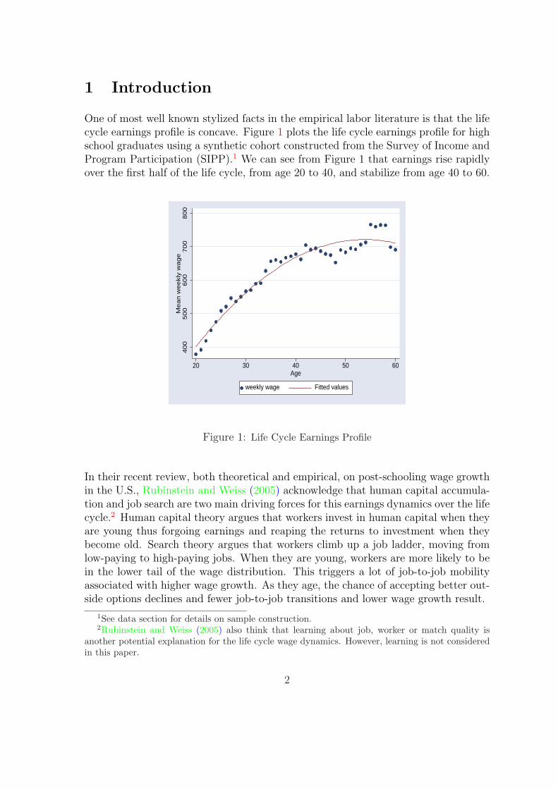
One of most well known stylized facts in the empirical labor literature is that the lifecycle earnings profile is concave. Figure 1 plots the life cycle earnings profile for highschool graduates using a synthetic cohort constructed from the Survey of Income andProgram Participation (SIPP).1 We can see from Figure 1 that earnings rise rapidlyover the first half of the life cycle, from age 20 to 40, and stabilize from age 40 to 60.

400

500

600

700

800

Mean w

eekly

wage

20 30 40 50 60Age

weekly wage Fitted values

Figure 1: Life Cycle Earnings Profile

In their recent review, both theoretical and empirical, on post-schooling wage growthin the U.S., Rubinstein and Weiss (2005) acknowledge that human capital accumula-tion and job search are two main driving forces for this earnings dynamics over the lifecycle.2 Human capital theory argues that workers invest in human capital when theyare young thus forgoing earnings and reaping the returns to investment when theybecome old. Search theory argues that workers climb up a job ladder, moving fromlow-paying to high-paying jobs. When they are young, workers are more likely to bein the lower tail of the wage distribution. This triggers a lot of job-to-job mobilityassociated with higher wage growth. As they age, the chance of accepting better out-side options declines and fewer job-to-job transitions and lower wage growth result.

1See data section for details on sample construction.2Rubinstein and Weiss (2005) also think that learning about job, worker or match quality is

another potential explanation for the life cycle wage dynamics. However, learning is not consideredin this paper.

2

This paper presents a life cycle model where both human capital investment andsearch intensity are endogenized to quantitatively examine the relative contributionsof both mechanisms to the earnings dynamics over the life cycle. The motivationof this unification is twofold. First, as pointed out by Rubinstein and Weiss (2005),it is important and interesting to study the relative contributions of human capitalaccumulation and job search to life cycle earnings growth since they have differentpolicy implications concerning training on the one hand and labor market mobilityon the other hand. Understanding which mechanism is more important can providetheoretical grounds and support for policy makers to design policies and programs toimprove workers’ welfare. To do this, a framework which incorporates both humancapital accumulation and job search is needed.

Second, there are interesting interactions between human capital investment andjob search behavior over the life cycle as briefly discussed in Rubinstein and Weiss(2005). In their paper, they provide a fairly simple exercise where workers decidehow much time to invest in human capital and receive exogenous job offers in theform of human capital rental rates. An interesting implication from their exercise isthat workers invest more in human capital than they would without job search andwith only a fixed rental rate of human capital. This is due to the upward drift in thedistribution of the human capital rental rate, which is inherent in the search model.However, their model may miss the interactions in the other direction. That is, searchbehavior may change if human capital accumulation is allowed. The intuition is sim-ple. Without human capital accumulation, the return to search is only realized for afixed level of human capital. With human capital accumulation, the return to searchis greater since it is now realized for growing human capital. Hence workers maytend to spend more effort on searching with human capital accumulation than with-out. Therefore, it is interesting to endogenize both human capital investment and jobsearch within a single framework to examine the joint interactions.

The literature on quantifying the relative contributions of human capital accumu-lation and job search to life cycle earnings growth is relatively new. It can be dividedinto papers that use reduced form empirical analysis and those that use structuralmodels. Using the first methodology, Mincer and Jovanovic (1979), Schonberg (2005),and Dustmann and Meghir (2005), among others, focus on using econometric methodsto control the endogeneity of job mobility and unobserved heterogeneity. In general,they find that general human capital is the most important source of wage growth.The return to firm-specific human capital is mixed and differentiated across countriesand skill groups. Job search accounts for 20 to 30% of total wage growth.

Within the structural model literature, the papers can be divided into 2 groups:papers that incorporate deterministic human capital accumulation into exogenoussearch models and those that allow for endogenous human capital accumulation inexogenous search models. Bunzel et al. (1999), Bagger et al. (2007), Barlevy (2005),Omer (2004), Yamaguchi (2006), and Pavan (2007) are included in the first group.Bunzel et al. (1999) allow for a linear human capital production function within Bur-

3

dett and Mortensen (1998)’s wage-posting framework where wages are allowed to growon the job linearly. They find that there is almost no human capital accumulation,especially for high school graduates using Danish data. Bagger et al. (2007) allowfor a piece-wise linear human capital production function to examine how earningsdynamics are related to interfirm competition due to search, human capital accumu-lation, and idiosyncratic production shock within Postel-Vinay and Robin (2002)’scounter-offer framework. They find that human capital accumulation is more impor-tant than job search early in the career for medium and high skilled workers. Omer(2004) allows for a linear human capital accumulation within a partial search modeland finds that on-the-job search contributes 4 times less than general experience tototal wage growth. Yamaguchi (2006) allows for a polynomial human capital accumu-lation process and focuses on wage bargaining between firms and workers. He findsthat human capital accumulation is more important and accounts for around 60% ofthe total wage growth over the first 10 years.

Compared to these papers, my paper differs in the following dimensions. First,these papers only allow for deterministic human capital accumulation and job offersarrive exogenously.3 In my paper, both human capital investment and search inten-sity are endogenized thus allowing for endogenous job arrival rates. Second, mostof these papers treat human capital accumulation and job search separately with nointeractions. Omer (2004) and Yamaguchi (2006) do discuss the interactions but theirmodels are restrictive in how human capital accumulation affects job search behav-ior. With human capital accumulation, the reservation wage (or match quality inYamaguchi (2006) is lower than without. However, in my model, the interactionsin both directions can be studied since both forces are endogenized. In particular,not only is the reservation rental rate lower, but the job arrival rate is higher withhuman capital accumulation than without. Third, these papers only focus on thewage growth over the first half of the life cycle within frameworks where workers liveinfinitely. My paper focuses on the earnings dynamics over the full life cycle withina life cycle framework.

Rubinstein and Weiss (2005) is included in the second group where only humancapital investment is endogenized. My paper takes a further step by explicitly model-ing both human capital investment and search intensity decisions within a relativelysimple search framework to examine the interactions between human capital invest-ment and job search. Jovanovic (1979) endogenizes both human capital investmentand search intensity. However, he primarily focuses on the relationship between thefirm-specific human capital and job separation within a matching framework.

In the model, workers face a non-degenerate distribution of the human capitalrental rate in the presence of labor market imperfections.4 Workers can improve their

3Pavan (2007) is an exception in the sense that he allows for the job arrival and job destructionrates to depend on a series of observable and unobservable characteristics.

4In this paper, I do not consider the firm’s problem, i.e., how the rental rate distribution isdetermined. However, this question is important and will be investigated in the future.

4

earnings over the life cycle by accumulating human capital and searching for betterrental rates. The expectation of rising rental rates through searching in the futuregives workers more incentive to invest in human capital. In the meantime, workerstend to spend more effort on searching for better jobs due to the reinforcement fromhuman capital accumulation. My preliminary results show that human capital in-vestment and job search working together are able to produce a concave life cycleearnings profile. Workers are willing to accept lower rental rates at the beginning oflife cycle in order to facilitate human capital formation. As more human capital isaccumulated, job search becomes more beneficial. These interactions between humancapital investment and job search cause a dramatic increase in earnings at the begin-ning of the life cycle. As the life cycle progresses, both job search and human capitalaccumulation slow down and so does earnings growth.

The structural model is estimated through indirect inference using synthetic co-horts constructed from the National Longitudinal Survey of Youth (NLSY) and theSurvey of Income and Program Participation (SIPP). I show that the search andhuman capital production function parameters can be identified using both earn-ings information and information on job-to-job transitions and unemployment-to-jobtransitions over the full life cycle. Preliminary results show that human capital ac-cumulation is more important in shaping the life cycle earnings profile, accountingfor 67-80% of the total earnings growth. Job search also plays a substantial role,accounting for 20-33% of the total growth.

The rest of the paper is organized as follows. The model is presented in Sec-tion 2. Section 3 discusses the identification and estimation strategies. Details onsample selection and construction of labor market histories are presented in Section4. Section 5 discusses estimation results and quantifies the relative contributions ofhuman capital accumulation and job search to life cycle earnings dynamics. Section6 concludes.

2 Model

2.1 The Environment

The model is built in the spirit of a Burdett and Mortensen (1998) search modeland a Ben-Porath (1967) human capital production model. Workers enter the labormarket unemployed at period 1, remain in the market until period T , and retire afterperiod T . They maximize their expected earnings over T periods in the labor marketby choosing how much market time to invest in human capital and how much effortto spend on search. At each period, they can be either unemployed or employed.

5

They may transit between unemployment and employment as well as from job tojob. Workers face a non-degenerate distribution of the rental rate of human capital,F (R), which is log-normally distributed. That is, ln(R) ∼ N(µ, σ2). Time is discrete.Workers discount the future at a rate β.

2.2 Human Capital Production Technology

Workers are endowed with an initial stock of human capital, h0, when they enter thelabor market. Human capital is assumed to be homogeneous and transferrable acrossjobs. Workers can only invest in human capital while on the job. Here human capitalrefers to skills that workers can only acquire through working. Human capital doesnot change during the course of unemployment. Following Heckman et al. (1998),human capital does not depreciate.

Assume a simplified Ben-Porath human capital production function Q(h, i), whereh is the current human capital stock and i is the fraction of market time allocated tohuman capital investment. Assume the production function Q(·, ·) is concave in bothh and i and takes the following specification

Q(h, i) = a(hi)α,

where 0 < α < 1 is a curvature parameter and a > 0 is a scale parameter whichrepresents learning ability. I assume learning ability is constant over time. Hence thelaw of motion for human capital for employed workers at period t is

ht+1 = ht + a(htit)α.

2.3 Search Technology

In the search literature, there are several ways of measuring search intensity: fractionof time devoted to job search (Seater (1977) and Jovanovic (1979)), number of appli-cations filled out or the number of job search methods used by a worker (Benhabiband Bull (1983) and Shimer (2004)), and search effort (Mortensen (2003), Chris-tensen et al. (2005), Lise (2005)). Search effort can include time and resources spenton search as well as anything else that affects the job offer arrival rate. In this paper,I follow Mortensen (2003) and Christensen et al. (2005) and use search effort as themeasure of search intensity.

Let λ(s) denote the job offer arrival rate, an increasing and concave function ofsearch effort s, with boundary conditions λ(0) = 0 and λ′s−→0 = +∞. Assume alinear production function for the job offer arrival rate, i.e. λ(s) = λs, where λ is a

6

search efficiency parameter. Let c(s) be the search cost function, increasing, strictlyconvex and twice differentiable, with boundary condition c(0) = c′s−→0 = 0. FollowingMortensen (2003) and Christensen et al. (2005), the search cost function takes thefollowing power form

c(s) =c0s

1+γ

1 + γ,

where c0 > 0 is a scale parameter and 1 + γ (γ > 0) is the elasticity of search costwith respect to search effort. Here the search cost refers to the pecuniary disutilityassociated with job search, not the opportunity cost of market time.

2.4 Worker’s Problem

The state variables upon which workers make decisions include the employment state,the current stock of human capital, and the current rental rate. Let Ut(h) denote thevalue of being unemployed at period t and with human capital h. Let Vt(h,R) bethe value of working at a firm offering a rental rate R at period t with human capitalh. The worker’s problem can be characterized recursively by two Bellman equations.The Bellman equation for an unemployed worker is

Ut(h) = maxs0t

bh− c(s0t ) + βλs0

t

∫max{Ut+1(h), Vt+1(h,R)}dF (R)

+β(1− λs0t )Ut+1(h)

s.t

0 ≤ λs0t ≤ 1 (1)

At period t, an unemployed worker receives some amount of compensation, bh whichdepends on his stock of human capital at that period. I assume b, the rental rateequivalent for the unemployed, is constant over time and independent of h. At thebeginning of period t, given his human capital, h, the worker must decide how mucheffort, s0

t , to expend on job search which in turn determines the job offer arrival rateat the end of period t. At the end of period t, with probability λs0

t , he receives a joboffer R from the offer distribution F (R). He has to immediately decide whether toaccept that offer by comparing the value of working at period t + 1 if accepts to thevalue of staying unemployed at period t + 1. With probability 1−λs0

t , he receives nooffer and hence stays unemployed at period t + 1.

The Bellman equation for an employed worker who works at a firm offering R

7

with human capital h at period t is

Vt(h,R) = max{s1

t ,it}Rh(1− it)− c(s1

t ) + β(1− δ)(1− λs1t )Vt+1(h

′, R)

+β(1− δ)λs1t

∫max{Vt+1(h

′, R′), Vt+1(h′, R)}dF (R′)

+βδUt+1(h′)

s.t

0 ≤ it ≤ 1,

0 ≤ λs1t ≤ 1

h′ = h + a(hit)α. (2)

At the beginning of period t, given his human capital stock h and rental rate R, anemployed worker has to decide not only how much effort s1

t to spend on searching fora better job but also how much time it to invest in human capital and thus earningsto forego. The worker receives earnings Rh(1− it) for period t and production, bothcommodity and human capital, then takes place. At the end of period t, the job canbe destroyed with probability δ in which case the worker returns to unemploymentat period t + 1. With probability (1− δ)λs1

t , the job is not destroyed and the workerreceives a new job offer R′ at the end of period t. The worker then must decidewhether to accept the new job offer R′ by comparing the value of working at the newjob at period t + 1 to that of staying with the current job at period t + 1 with thenew human capital h′. With probability (1− δ)(1−λs1

t ), the job is not destroyed andthe worker receives no offers and stays with the current job at period t + 1.5 Humancapital grows due to investment and human capital at period t + 1 is determined bythe law of motion.

It can be shown from backward induction that Ut(h) is increasing in h and Vt(h,R)is increasing in both h and R. Given these properties of the value functions, unem-ployed workers adopt the following reservation rental rate strategy: only offers thatare at least as good as the reservation rental rate, denoted by φt(h) and determinedby Ut(h) = Vt(h, φt(h)), are accepted. For employed workers, the reservation rentalrate, at which workers are indifferent between accepting the new offer and stayingwith the current job, is the current rental rate, since human capital is general andtransferable between jobs. Using the reservation rental rate strategies, the Bellman

5Since the model is non-stationary, it is possible that workers may find that quitting to unem-ployment is worthwhile in some cases. However, I find that they barely choose to do so after allowingvoluntary quit to unemployment. Hence I abstract that choice here for simplicity.

8

equations (1) and (2) can be simplified as follows.

Ut(h) = maxs0t

bh− c(s0t ) + βλs0

t

∫

φt+1(h)

(Vt+1(h,R′)− Ut+1(h)) dF (R′)

+βUt+1(h)

s.t.

0 ≤ λs0t ≤ 1. (3)

Vt(h,R) = max{s1

t ,it}Rh(1− it)− c(s1

t ) + β(1− δ)Vt+1(h′, R) + βδUt+1(h

′)

+β(1− δ)λs1t

∫

R

(Vt+1(h′, R′)− Vt+1(h

′, R)) dF (R′)

s.t.

0 ≤ it ≤ 1,

0 ≤ λs1t ≤ 1

h′ = h + a(hit)α. (4)

2.5 Analysis

Assuming interior solutions, the following three first order conditions characterize thesolutions to the model:

c′(s0t ) = βλ

∫

φt+1(h)

(Vt+1(h,R′)− Ut+1(h)) dF (R′), (5)

c′(s1t ) = β(1− δ)λ

∫

R

(Vt+1(h′, R′)− Vt+1(h

′, R)) dF (R′), (6)

Rh = β∂h′

∂it

(δ∂Ut+1(h

′)∂h′

+ (1− δ)∂Vt+1(h

′, R)

∂h′

+(1− δ)λs1t

∫

R

(∂Vt+1(h

′, R′)∂h′

− ∂Vt+1(h′, R)

∂h′

)dF (R′)

). (7)

Equation (5) characterizes the optimal search intensity for the unemployed. Theleft hand side of the equation is the marginal cost of search and the right hand sideis the marginal return to search. The interactions between human capital investmentand job search lie in that unemployed workers tend to spend more effort on searchand lower their reservation rates with human capital accumulation than without. Theintuition is simple. Working is more attractive than staying unemployed, if human

9

capital accumulation is allowed. On the one hand, workers receive constant compen-sation bh and see no growth in human capital while unemployed. On the other hand,they may augment their human capital and locate better outside offers while working.This encourages unemployed workers to exit unemployment as quickly as possible bysearching more intensively and lowering their reservation rates. Hence s0

t is higherand the reservation rate φt+1(h) is lower than they would be without human capitalgrowth. s0

t is increasing in h, because the marginal returns to search are higher forworkers with more human capital.6

Equation (6) characterizes the optimal search intensity for the employed workers.The on-the-job search intensity with human capital growth is higher than withoutsince the marginal return to search is higher than it would be with no human capitalgrowth.7 s1

t is increasing in h because search is more valuable for individuals withmore human capital as the right hand side is increasing in h′ which in turn is increas-ing in h. As R increases, the marginal return to search decreases since the probabilityof reaping the gains due to search becomes smaller. Hence s1

t is decreasing in R.Equation (7) characterizes the optimal investment in human capital. The invest-

ment is decreasing in h due to the concavity of the human capital production function.The right hand side is the expected marginal return to human capital investment. Itincludes 3 parts. The first term is the marginal return to investment if workers endup unemployed next period. The second term is the marginal return to investmentif workers stay with the same job. The last term is a “bonus” due to search, whichis the expected marginal return to investment if workers switch jobs. To see howhuman capital investment interacts with job search, set δ equal to 0 for a moment. Ina pure human capital world where there is no job search, the third term drops out andR does not matter for the investment decision. This is because what workers foregotoday per unit of human capital is the same as what they receive tomorrow. However,with job search, the marginal return to human capital investment now includes boththe second and the third terms. Hence the investment in human capital is greaterwith job search than without. Meanwhile with job search, the investment in humancapital is decreasing in R. This is because the “bonus” term is a decreasing functionof R. The higher the R is, the less likely workers receive the “bonus”. This is generalas long as δ is small and b is relatively low compared to the distribution of the rentalrate.

6This can be easily proved for period T − 1. I assume without loss of generality that UT+1 =VT+1 = 0. In this case, UT (h) = bh, VT (h,R) = Rh, and φT (h) = b. After substituting these intoequation (5), the right hand side becomes βλh

∫b(R′ − b)dF (R′) which is increasing in h, as long as

some of the rental rates are higher than b.7This is clear for period T − 1, since UT (h) = bh and VT (h,R) = Rh. The marginal return to

search with human capital accumulation is β(1− δ)λh′∫

R(R′ −R)dF (R′) which is greater than the

counterpart without human capital growth, β(1− δ)λh∫

R(R′ −R)dF (R′) since h′ > h.

10

2.6 Numerical Illustration

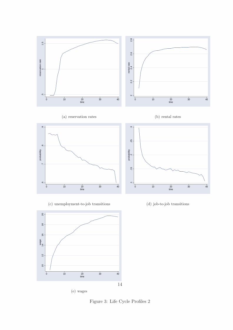
Due to the intractability of the analytical solutions to the structural model, I presenta numerical example in this section to demonstrate how the model works and howhuman capital accumulation interacts with job search over the life cycle. To do this,I solve a 40-period model for a set of parameters listed in Table 1. The model isthen simulated to generate a random sample of size of 20,000. Life cycle profiles ofsearch intensities and human capital investment and those of wages and transitionsare plotted in Figures 2 and 3.

Generally speaking, the search intensities, both for the unemployed and employed,decrease as workers age. Search intensity, plotted in panel (a) of Figure 2, for theunemployed is relatively flat. This is mainly because human capital only accumulateson the job. As long as investment in human capital is still beneficial, unemployedworkers would like to work rather than stay unemployed. The search intensity onthe job, plotted in panel (b) of Figure 2, is smaller than the counterpart for theunemployed. This implies the job arrival rate on the job is lower than that for theunemployed workers, which is consistent with the findings in the search literature.The search intensity on the job is decreasing over time because the values of outsideoptions decrease as workers move from low-paying to high-paying jobs. Human cap-ital investment, plotted in panel (c) of Figure 2, is also declining over time. At theend of the life cycle, workers barely invest in human capital. The curvature of thehuman capital investment depends on α. The larger α is, the more investment inhuman capital occurs at the beginning of the life cycle.

The reservation rate for the unemployed workers is generally increasing over time,as shown in panel (a) of Figure 3. At the beginning of the life cycle, workers wouldlike to accept any rental rate and set their reservation rates equal to the minimumrental rate in the distribution under the current parameterization. This is becauseinvestment in human capital at the beginning of the life cycle is so valuable thatworkers would like to accept any job to start accumulating human capital. As humancapital accumulates over time, the value of being unemployed increases and the incen-tive to invest in human capital declines. This causes the reservation rate to increase.The reservation rate decreases slightly when the life cycle comes to the end, equalto b at the last period. The rental rate, plotted in panel (b) of Figure 3, rises overtime with a dramatic increase at the beginning of the life cycle and then stabilizes.This causes a big drop in the job-to-job transition rate at the beginning of the lifecycle, as shown in panel (d) of Figure 3, along with the declining search intensity onthe job. The unemployment-to-job transition rate, plotted in panel (c) of Figure 3, isalso decreasing over time. Most of the decline is due to the increase of the reservationrate since the search intensity for the unemployed is relatively flat over time. As aresult of both human capital accumulation and job search, as shown in panel (e) ofFigure 3, wages increase over time and with a concave-shape.

The interactions between human capital investment and job search can be shown

11

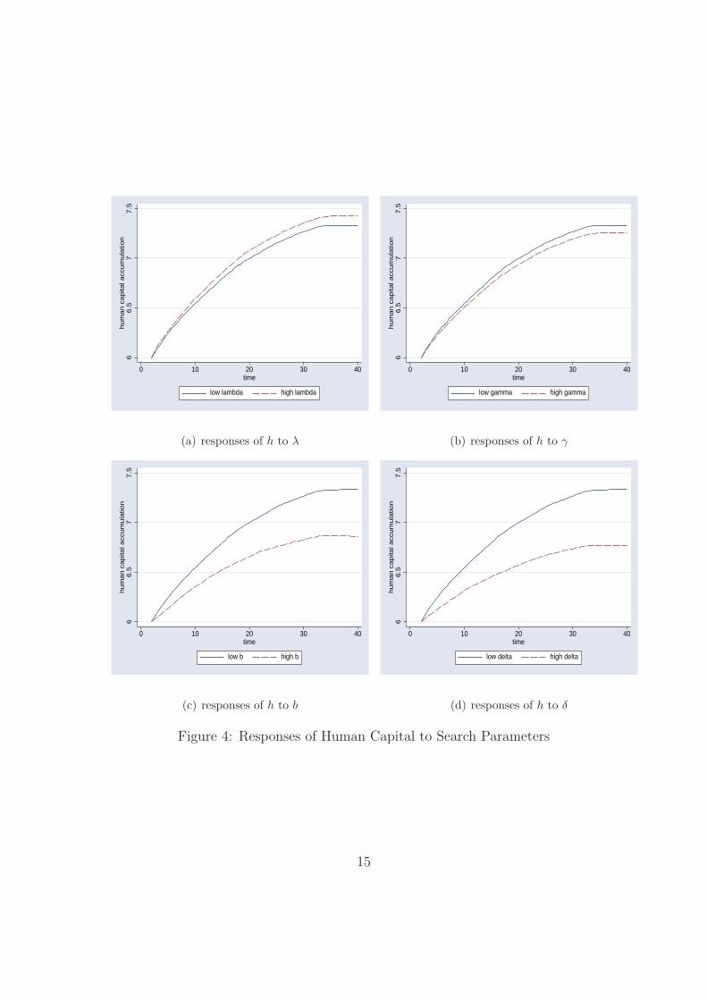
by examining how human capital investment responds to changes in the search pa-rameters on the one hand and how search behavior responds to changes in the humancapital production parameters. A high λ results in more investment in human capi-tal and more human capital accumulated over time, as shown in panel (a) of Figure4. This is because a high λ results in more unemployment-to-job and job-to-to jobtransitions increasing the expectation of an increase in the rental rate over the lifecycle, holding everything else constant. For γ the pattern is reversed. A high γ meanshigh search costs that discourage workers from searching for better outside options.Therefore workers make fewer unemployment-to-job and job-to-job transitions andless investment in human capital results, as shown in panel (b) of Figure 4. Theparameters b and δ work the same way as γ. A high b increases the value of beingunemployed and discourages workers from exiting unemployment. A high δ increasesthe probability of workers going back to unemployment and lowers the return to hu-man capital investment. In both cases, less human capital accumulation results, asplotted in panels (c) and (d) of Figure 4, respectively.

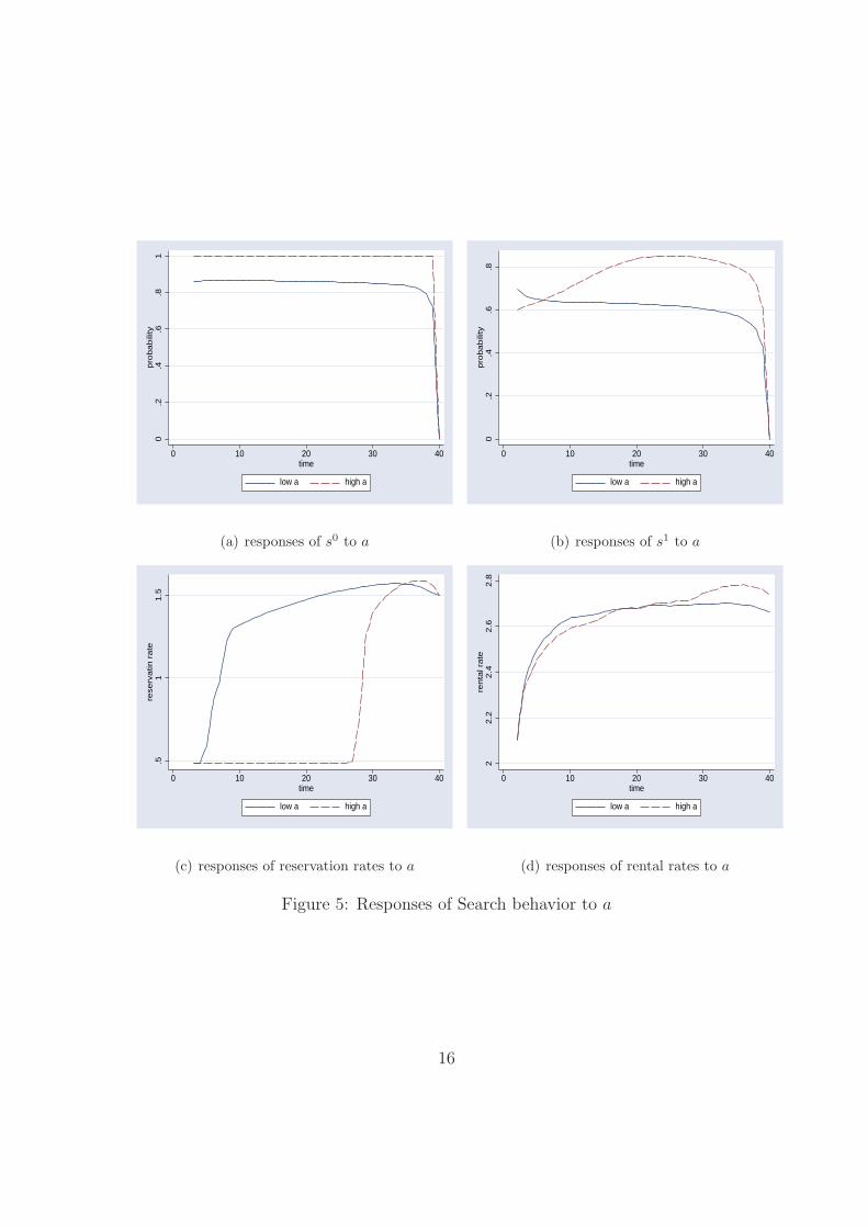
Changes in the human capital production parameters also affect search behaviorover the life cycle. A high value for learning ability, a, induces workers to investmore in human capital. This causes workers to spend more effort in searching whileunemployed to exit unemployment as quickly as possible, as plotted in panel (a) ofFigure 5. It is interesting that with a high a the search intensity on the job becomeslower at the beginning of the life cycle and then higher than that with a low a. Thisis mainly because a high a also induces more investment in human capital at thebeginning of the life cycle. Workers choose to substitute search intensity for humancapital investment because they can not afford to increase both at the same time. Asworkers accumulate more human capital, the search intensity on the job surpassesthat with a low a due to the positive interactions between search and human capitalaccumulation, as shown in panel (b) of Figure 5. The reservation rate with a higha is lower than that with a low a and is at the lower bound of the rental rates forlonger period of time. This is due to more investment in human capital associatedwith a high a. At the end of the life cycle, with a high a, more human capital ac-cumulates and the reservation rate becomes higher than that with a low a.Finally,with a high a, the average rental rate is lower during the first half of the life cycleand then overtakes that with a low a at the end of life cycle. This is a result of boththe reservation rate and search intensity on the job exhibiting similar patterns overthe life cycle. The parameter α works the same way as a does. A high α inducesmore investment in human capital at the beginning of the life cycle. Thus, in order totake advantage of this, workers want to exit unemployment as quickly as possible byincreasing search intensity and lowering the reservation rate, and to substitute searchintensity for human capital investment while working early in the life cycle.

12

λ c γ b δ a α h0 µ σ β T

0.57 1.0 4.0 1.5 0.2 0.08 0.6 6.0 0.7 0.3 0.96 40

Table 1: Parameters Used for Numerical Illustrations

0.2

.4.6

.8pro

babili

ty

0 10 20 30 40time

(a) search intensity while unemployed

0.2

.4.6

.8pro

babili

ty

0 10 20 30 40time

(b) on-the-job search intensity

0.1

.2.3

fract

ion

0 10 20 30 40time

(c) human capital investment

66.5

77.5

hum

an c

apita

l

0 10 20 30 40time

(d) human capital accumulation

Figure 2: Life Cycle Profiles 1

13

.51

1.5

rese

rvatio

n r

ate

0 10 20 30 40time

(a) reservation rates

22.2

2.4

2.6

2.8

renta

l rate

0 10 20 30 40time

(b) rental rates

.6.7

.8.9

pro

babili

ty

0 10 20 30 40time

(c) unemployment-to-job transitions

.1.1

5.2

.25

.3pro

babili

ty

0 10 20 30 40time

(d) job-to-job transitions

10

12

14

16

18

20

wage

0 10 20 30 40time

(e) wages

Figure 3: Life Cycle Profiles 2

14

66.5

77.5

hum

an c

apita

l acc

um

ula

tion

0 10 20 30 40time

low lambda high lambda

(a) responses of h to λ

66.5

77.5

hum

an c

apita

l acc

um

ula

tion

0 10 20 30 40time

low gamma high gamma

(b) responses of h to γ

66.5

77.5

hum

an c

apita

l acc

um

ula

tion

0 10 20 30 40time

low b high b

(c) responses of h to b

66.5

77.5

hum

an c

apita

l acc

um

ula

tion

0 10 20 30 40time

low delta high delta

(d) responses of h to δ

Figure 4: Responses of Human Capital to Search Parameters

15

0.2

.4.6

.81

pro

babili

ty

0 10 20 30 40time

low a high a

(a) responses of s0 to a

0.2

.4.6

.8pro

babili

ty

0 10 20 30 40time

low a high a

(b) responses of s1 to a

.51

1.5

rese

rvatin

rate

0 10 20 30 40time

low a high a

(c) responses of reservation rates to a

22.2

2.4

2.6

2.8

renta

l rate

0 10 20 30 40time

low a high a

(d) responses of rental rates to a

Figure 5: Responses of Search behavior to a

16

0.2

.4.6

.81

pro

babili

ty

0 10 20 30 40time

low alpha high alpha

(a) responses of s0 to α

0.2

.4.6

.8pro

babili

ty

0 10 20 30 40time

low alpha high alpha

(b) responses of s1 to α

.51

1.5

rese

rvatin

rate

0 10 20 30 40time

low alpha high alpha

(c) responses of reservation rates to α

22.2

2.4

2.6

2.8

renta

l rate

0 10 20 30 40time

low alpha high alpha

(d) responses of rental rates to α

Figure 6: Responses of Search behavior to α

17

3 Identification and Estimation

The structural parameters of interest include 5 parameters related to search friction(λ, δ, b, c, and γ), 2 human capital production function parameters (a and α), theinitial human capital level (h0), and 2 distribution parameters for the rental rate (µand σ). For this version, I assume workers are ex ante homogeneous in terms of theinitial stock of human capital h0 and learning ability a. This is mainly because thegoal of this paper is to examine the evolution of earnings over the life cycle for arelatively homogeneous group, white male high school graduates.

3.1 Identification

One of the key issues for the estimation is how to separately identify the search andhuman capital production function parameters, since these two forces interact witheach other over the life cycle. In the search literature, the search parameters usuallyare identified using wage information, information on unemployment durations andjob durations, and information on job-to-job transitions. The key idea of this paperin estimating search parameters is to use the information on unemployment-to-jobtransitions and job-to-job transitions over the full life cycle, especially the informationof older workers. The idea is as follows. The model predicts that the investment inhuman capital decreases as workers age. Older workers experience almost no humancapital growth. However, they still make job-to-job transitions especially when theircurrent jobs have a low rental rate. Hence, the search parameters can be identified byexamining how the job-to-job transitions, especially for the older workers, respondsto observed characteristics, for example, experience, job tenure, and wages. Sincesearch intensity is not observed in data, λ, c, and γ can only be identified up to scaleunless c is normalized (Christensen et al. (2005)). Here in this paper I normalize c to1 for identification purposes.

In the human capital literature, the human capital production function parametersare estimated using information on wage growth, because wage growth only comesfrom human capital investment in human capital models.8 However, wage growthin my model is a result of both human capital accumulation and job search throughjob-to-job transitions. Nevertheless, on the same job, wages grow solely due to humancapital accumulation. Hence the information on within-job wage growth can help toidentify the human capital production function parameters, a and α. It is well knownin the human capital literature that one cannot separately identify the level of initialhuman capital from the rental rate. Usually the rental rate is normalized to someparticular value so that it is possible to interpret human capital in a pecuniary sense.

8For example, see Heckman et al. (1998), Hugget et al. (2004), Heckman (1976), and Brown(1976).

18

The integration of job search and human capital accumulation in this paper does notresolve this issue either. In fact, in addition to the non-separation between h0 and µ,b and a can not be separated from h0 either, as shown in the following proposition.

Proposition 1 Given λ, γ, α, and σ, for any κ > 0,

h′0 = h0κ , µ′ = µ− ln(κ)

b′ = b/κ , a′ = aκ1−α

the two sets of parameters {h0, µ, b, a} and {h′0, µ′, b′, a′} yield the same behavior

(search intensities and human capital investment) with T = 2.

Proof. See the Appendix.The non-separation between h0 and µ and between h0 and b results from the

multiplicative period earnings functions, hR(1 − i) and hb, and the fact that h isnot observed. For decisions on search intensity, what really matters is the relativelocation in the rental rate distribution, which is not affected by the scaling. Recallthat within-job wage growth is used to identify the human capital production functionwhere a acts as the intercept and α acts as the slope of wage growth. Taking thedifference of wages drops the intercept term a, which leads to the identification for αbut not for a. Hence a has to adjust relative to h0.

To confirm that the scaling is also true in a more general setting, I solve andsimulate a 40-period model based on two sets of parameters that have the propertiesdescribed in the above proposition. The results (in Figures 7 and 8) show that humancapital investment and search intensity, as well as the transition and wage profiles,are almost identical under these two sets of parameters. Parameterizations are list inTable 2.

In this paper, the initial human capital h0 is normalized to 100. The model periodis set to a quarter (13 weeks). The discount factor β is then fixed following theconvention in the literature such that β = 1/(1 + r) where r is the quarterly risk-freeinterest rate. The quarterly interest rate is derived from an annual interest rate of 4%.The rest of the parameters are then estimated via indirect inference (Gourieroux et al.(1993)). Indirect inference is a generalization of the method of simulated moments.The main idea is to find a set of structural parameters that minimize the distancebetween a set of moments from the real data and the model-predicted counterpartsof these moments based on simulated data from the structural model. The set ofmoments that are matched can be viewed as a set of auxiliary parameters from a setof auxiliary models. These auxiliary models can be structural or just reduced formsand they should capture the main features of the original structural model.

19

0.2

.4.6

.8jo

b a

rriv

al ra

te o

ff the job

0 10 20 30 40time

h0=6 h0=3

(a) search intensity while unemployed

0.2

.4.6

.8o

n−

the

−jo

b a

rriv

al ra

te

0 10 20 30 40time

h0=6 h0=3

(b) on-the-job search intensity

0.1

.2.3

.4h.c

. in

vestm

ent

0 10 20 30 40time

h0=6 h0=3

(c) human capital investment

10

15

20

wages

0 10 20 30 40time

h0=6 h0=3

(d) wages

Figure 7: Decisions and Profiles under 2 Parameterizations

20

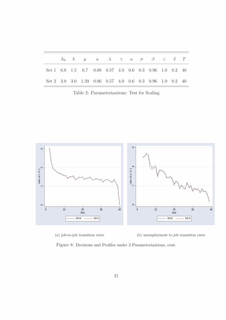
h0 b µ a λ γ α σ β c δ T

Set 1 6.0 1.5 0.7 0.08 0.57 4.0 0.6 0.3 0.96 1.0 0.2 40

Set 2 3.0 3.0 1.39 0.06 0.57 4.0 0.6 0.3 0.96 1.0 0.2 40

Table 2: Parameterizations: Test for Scaling

0.1

.2.3

rate

of

j−2

−j

0 10 20 30 40time

h0=6 h0=3

(a) job-to-job transition rates

.6.7

.8.9

rate

of

u−

2−

j

0 10 20 30 40time

h0=6 h0=3

(b) unemployment to job transition rates

Figure 8: Decisions and Profiles under 2 Parameterizations, cont.

21

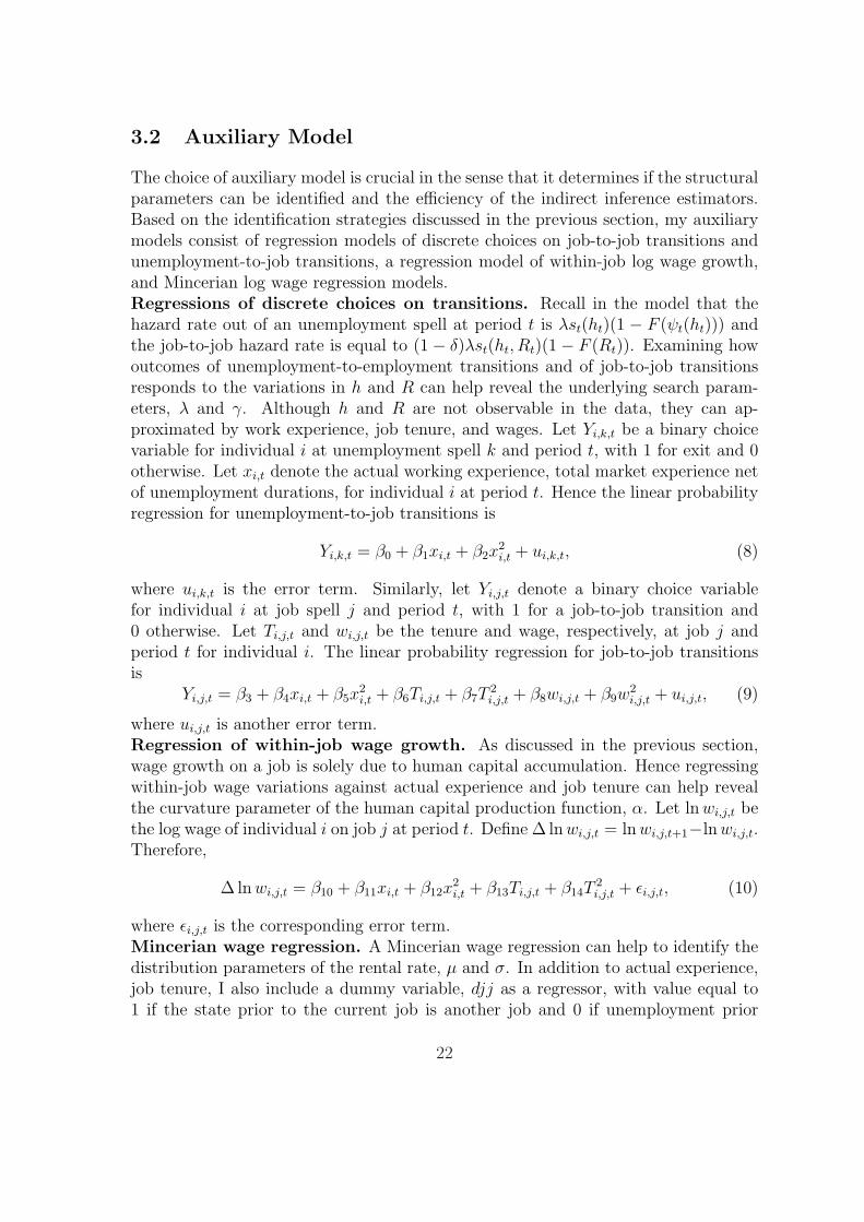
3.2 Auxiliary Model

The choice of auxiliary model is crucial in the sense that it determines if the structuralparameters can be identified and the efficiency of the indirect inference estimators.Based on the identification strategies discussed in the previous section, my auxiliarymodels consist of regression models of discrete choices on job-to-job transitions andunemployment-to-job transitions, a regression model of within-job log wage growth,and Mincerian log wage regression models.Regressions of discrete choices on transitions. Recall in the model that thehazard rate out of an unemployment spell at period t is λst(ht)(1 − F (ψt(ht))) andthe job-to-job hazard rate is equal to (1− δ)λst(ht, Rt)(1− F (Rt)). Examining howoutcomes of unemployment-to-employment transitions and of job-to-job transitionsresponds to the variations in h and R can help reveal the underlying search param-eters, λ and γ. Although h and R are not observable in the data, they can ap-proximated by work experience, job tenure, and wages. Let Yi,k,t be a binary choicevariable for individual i at unemployment spell k and period t, with 1 for exit and 0otherwise. Let xi,t denote the actual working experience, total market experience netof unemployment durations, for individual i at period t. Hence the linear probabilityregression for unemployment-to-job transitions is

Yi,k,t = β0 + β1xi,t + β2x2i,t + ui,k,t, (8)

where ui,k,t is the error term. Similarly, let Yi,j,t denote a binary choice variablefor individual i at job spell j and period t, with 1 for a job-to-job transition and0 otherwise. Let Ti,j,t and wi,j,t be the tenure and wage, respectively, at job j andperiod t for individual i. The linear probability regression for job-to-job transitionsis

Yi,j,t = β3 + β4xi,t + β5x2i,t + β6Ti,j,t + β7T

2i,j,t + β8wi,j,t + β9w

2i,j,t + ui,j,t, (9)

where ui,j,t is another error term.Regression of within-job wage growth. As discussed in the previous section,wage growth on a job is solely due to human capital accumulation. Hence regressingwithin-job wage variations against actual experience and job tenure can help revealthe curvature parameter of the human capital production function, α. Let ln wi,j,t bethe log wage of individual i on job j at period t. Define ∆ ln wi,j,t = ln wi,j,t+1−ln wi,j,t.Therefore,

∆ ln wi,j,t = β10 + β11xi,t + β12x2i,t + β13Ti,j,t + β14T

2i,j,t + εi,j,t, (10)

where εi,j,t is the corresponding error term.Mincerian wage regression. A Mincerian wage regression can help to identify thedistribution parameters of the rental rate, µ and σ. In addition to actual experience,job tenure, I also include a dummy variable, djj as a regressor, with value equal to1 if the state prior to the current job is another job and 0 if unemployment prior

22

to the current job. The model predicts that on average wages following job-to-jobtransitions are higher than those following unemployment. Let ln wi,j,t be the logwage at period t for individual i at job j. Hence,

ln wi,j,t = β15 + β16xi,t + β17x2i,t + β18Ti,j,t + β19T

2i,j,t + β20djji,j,t + νi,j,t. (11)

Regressions of initial wages and initial job-to-job transitions. Given theassumption of the common initial human capital among the same cohort, variationsof the initial wages and initial job-to-job transitions of the first job at period 2 solelycome from the variation of R and can help to identify the dispersion of the rentalrate distribution, σ. The initial wages of the first jobs at period 2 are also helpful toidentify the mean of the rental rate distribution, µ. Let ln wi,2 be the logarithm ofthe wage of the first job at period 2 for individual i.9 Let Yi,2 be a binary variableindicating a job-to-job transition from the first job at period 2 for individual i. LetTi,1 be the total tenure of the first job for individual i. Therefore,

ln wi,2 = β21 + β22Ti,1 + β23T2i,1 + ε1

i (12)

Yi,2 = β24 + β25Ti,1 + β26T2i,1 + β27wi,2 + β28w

2i,2 + ε2

i (13)

Additional moments. The job destruction rate, δ, is assumed in the model to bethe same for everyone and constant over time. Hence a consistent estimator of δ isthe average fraction of workers who are laid off over time. The rental rate equivalentfor the unemployed, b, affects the individual reservation rental rate and is equal tothe reservation rental rate at period T . Hence the minimum wage at period T , wT ,among those who just come out of unemployment can help to identify b.Summary. Denote θ as the set of parameters of interest that need to be estimated.That is θ = {λ, b, γ, a, α, µ, σ}.10 Denote ρ as the vector of auxiliary parameters,whose consistent estimator based on the real data is ρ. Here ρ includes all theregression coefficients β0 to β28 from equations (8) to (13) plus one additional moment,wT . In total, there are 30 moments that I seek to match using the structural model.Let ρ(θ)s be the consistent estimator of ρ from the artificial data generated fromone simulation of the structural model, indexed by s. Let ρ(θ) be the average of Ssimulations, ρ(θ) = (1/S)ΣS

s=1ρ(θ)s. Then the consistent estimator of θ, via indirectinference, is given by

θ = arg min(ρ(θ)− ρ)′W ∗(ρ(θ)− ρ), (14)

where W ∗ is the optimal weighting matrix, which is equal to the inverse of the co-variance matrix of ρ, V ar(ρ)−1. The minimization is implemented using simulated

9Every one in the model starts from unemployment at the first period. The initial wages areavailable from the second period, if any.

10The job destruction rate δ is set to match the empirical counterpart and not included in theestimation routine.

23

true values full life cycle first 25 years 20+20

λ 0.57 0.57 0.92 0.59

b 1.5 1.51 1.64 1.51

γ 4.0 4.09 5.97 4.63

a 0.08 0.08 0.08 0.08

α 0.6 0.60 0.57 0.6

h0 6.0 fixed fixed fixed

µ 0.7 0.70 0.60 0.69

σ 0.3 0.30 0.33 0.3

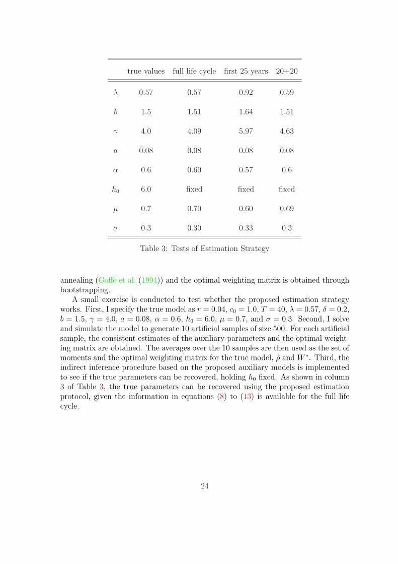
Table 3: Tests of Estimation Strategy

annealing (Goffe et al. (1994)) and the optimal weighting matrix is obtained throughbootstrapping.

A small exercise is conducted to test whether the proposed estimation strategyworks. First, I specify the true model as r = 0.04, c0 = 1.0, T = 40, λ = 0.57, δ = 0.2,b = 1.5, γ = 4.0, a = 0.08, α = 0.6, h0 = 6.0, µ = 0.7, and σ = 0.3. Second, I solveand simulate the model to generate 10 artificial samples of size 500. For each artificialsample, the consistent estimates of the auxiliary parameters and the optimal weight-ing matrix are obtained. The averages over the 10 samples are then used as the set ofmoments and the optimal weighting matrix for the true model, ρ and W ∗. Third, theindirect inference procedure based on the proposed auxiliary models is implementedto see if the true parameters can be recovered, holding h0 fixed. As shown in column3 of Table 3, the true parameters can be recovered using the proposed estimationprotocol, given the information in equations (8) to (13) is available for the full lifecycle.

24

3.3 Data Restrictions

My primary choice of data for the analysis is the NLSY from 1979 to 2004.11 Itprovides information on the job market history for around 20 to 25 years. Oneinteresting question is whether the proposed estimation strategy still works, giveninformation on only the first half of the life cycle is available as in the NLSY. To seethis, I conduct another exercise where only the information from the first 25 years isused in the estimation. The model specification is the same as the previous one. As wecan see from column 4 in Table 2, not all of the parameters are recovered, especiallythe search parameters, λ, b, and γ. This confirms that information for older workersis important to identify the search parameters as discussed in the previous section.The human capital production parameters, a and α, are almost recovered. This ismainly because younger workers undergo most of the investment in human capital.

To address this issue, I augment the NLSY with another panel data set, theSIPP. The most recent panel for the SIPP runs from 1996 to 2000. It providesdetailed information for every job held by respondents age 15 and over as of 1996over the survey period. I augment the auxiliary models with two extra regressions,the counterparts of regressions (9) and (11) for older workers. However, since theSIPP panel is a stock sample and short, job tenure and actual working experiencecan not be constructed. Hence, I replace actual working experience with potentialexperience and drop the job tenure in the these two regressions. The two regressionsfor the old workers are

Yi,j,t = β29 + β30exi,t + β31ex2i,t + β32wi,j,t + β33w

2i,j,t + ui,j,t, (15)

andln wi,j,t = β34 + β35exi,t + β36ex

2i,t + νi,j,t. (16)

where exi,t is the potential experience of individual i at period t.To summarize, my final auxiliary models for the indirect inference includes re-

gressions for two age groups, regressions (8) to (13) for the first half of the life cycle(the first 20 years in the NLSY), and regressions (15) and (16) for the second halfof the life cycle (age 40 to 60 in the SIPP). I conduct another exercise to test if therevised estimation strategy works due to the data limitations. The results are shownin column 5 of Table 3. Almost all of the parameters can be recovered except γ.At this stage, I can not tell if this is an upward bias due to the limited informationused in the regressions for the older group or just one randomization. Full sets ofMonte-Carlo exercises will be conducted to examine the properties of the estimatorunder 3 different scenarios: the full life cycle, only the first half, and the first halfplus limited information from the second half.

11See the data section for details on data issues.

25

4 Data

As discussed in the Estimation section, the identification strategy depends on havingboth wage information and information on unemployment-to-job transitions and job-to-job transitions over the full life cycle. There is not a single existing data set thatprovides all this information. My strategy is then to construct a synthetic cohortas consistent as possible from more than one panel data set. The two panel datasets I use are the NLSY and the SIPP. The NLSY consists of 12,686 individuals whowere 14 to 21 years old as of January 1979. It contains a nationally representativecore random sample, an oversample of blacks and Hispanics, and a special militaryoversample. Respondents have been interviewed since 1979 roughly once a year until1994 and once every two years after 1994. Detailed information on employment andschooling has been collected.

The SIPP survey is a continuous series of national panels with the first panel start-ing from 1984. For the 1984-1993 period, a new panel of households was introducedeach year in February. A 4-year panel was introduced in April 1996. The redesignabandoned the overlapping panel structure of the earlier SIPP, but maintained alarger sample size, with an initial sample size of 40,188 households. The 1996 panel isused for the analysis in this paper. The SIPP sample is a multistage-stratified sam-ple of the U.S. civilian non-institutionalized population. All household members 15years old and over are interviewed by self-response or proxy response every 4 months.Core information on labor force, program participation and income for the past 4months is asked at each interview. Both data sets provide instruments with whichjobs can be linked across interviews and thus individual labor market histories canbe constructed.

4.1 Sample Selection

In both data sets, I select only white males who are high school graduates and donot pursue further schooling. In the NLSY, I select only those who graduated fromhigh school after 1978, since reconstructing employment histories prior to 1978 is notpossible in the NLSY, and before 1984 in order to have more homogeneous cohorts. Inthe SIPP, I restrict the sample to those who were high school graduates as of January1996.

In both samples, a job is defined as an employment relationship that consists of atleast 35 hours a week12 and lasts longer than 4 weeks. In the NLSY, these full-timejobs have to start within three years after high school graduation to guarantee the

12The focus on full-time jobs is standard in the literature. See, for example, Bowlus et al. (2001),Eckstein and Wolpin (1995), Wolpin (1992), Yamaguchi (2006), Topel and Ward (1992), Rendon(2006).

26

school-to-work transition.13 If the first full-time job happens to surround the gradu-ation date, it is used as the first spell only if it is held at least 2 months longer aftergraduation. This eliminates temporary or summer jobs held while still in school. Todeal with overlapping jobs, I drop those jobs that are covered entirely by other longerjobs. For those jobs that only overlap in part, I replace the starting dates of the laterjobs with the stopping dates of the earlier jobs. In both samples, if a job is indicatedas still ongoing at the last interview, the job is right-censored. In the NLSY sample,the censoring rate is quite low, about 7.7% due to the long panel. The censoring ratefor the SIPP sample is around 67%.

Weekly wages are used as earnings and converted to 2000 dollars in both samples.In the NLSY, respondents are asked the time unit of rate of pay and correspondingrate of pay. If an individual is not paid weekly, the rate of pay is then converted toa weekly wage using hours information. In the SIPP, a monthly wage is recorded.Hence, a weekly wage is then equal to the monthly wage divided by the actual weeksworked for that particular month. In both samples, wages are trimmed 1% at the topand bottom of the distributions.

Those who had ever been self-employed, family workers, served in military, orretired are excluded in both samples. The final sample of analysis includes 552 in-dividuals and 2974 full-time jobs from the NLSY and 5109 individuals and 7575full-time jobs from the SIPP.

4.2 Quarterly Histories

The model period is a quarter (13 weeks). The quarterly labor market histories sincehigh school graduation are constructed for the two samples. The quarterly historiesare constructed according to the following rules.

First, I set the calendar quarter that contains the high school graduation date asthe first quarter in the labor market. This is in line with Wolpin (1992) and Ecksteinand Wolpin (1995). Second, employment states are determined based on the majoractivity occurring during a particular calendar quarter. In the literature, there aregenerally two ways to construct quarterly histories. One is to use the informationat the first week of a particular quarter. The other is to use the major activity ofa particular quarter.14 I follow the latter in this paper. A worker is classified asemployed, if he works most of the time, greater than 7 weeks, during a particularquarter. Otherwise, he is unemployed. Third, the job of the quarter is defined as theone that a worker stays with the longest during that quarter, given he is employedduring that quarter. The wage on this job during that quarter is then defined as the

13See Bowlus et al. (2001) for details.14Yamaguchi (2006) and Rendon (2006) use the former. Topel and Ward (1992) and Wolpin

(1992) use the latter.

27

wage for the quarter. Fourth, the quarterly transitions are determined based on theemployment states and jobs held during two consecutive quarters. A worker makesan unemployment-to-job transition if he is unemployed at the current quarter andemployed at the next quarter. A worker makes a job-to-job transition if he changesjobs between two quarters.

4.3 Sample of Analysis

Suppose individuals expect to work in the labor market for 40 years (160 quarters).The sample of analysis is a synthetic cohort which is composed of the NLSY cohort(the first 20 years) and the SIPP cohort which includes individuals who are 40 to60 between 1996 and 2000. The combined quarterly market histories from these twocohorts are then used for the estimation and analysis.

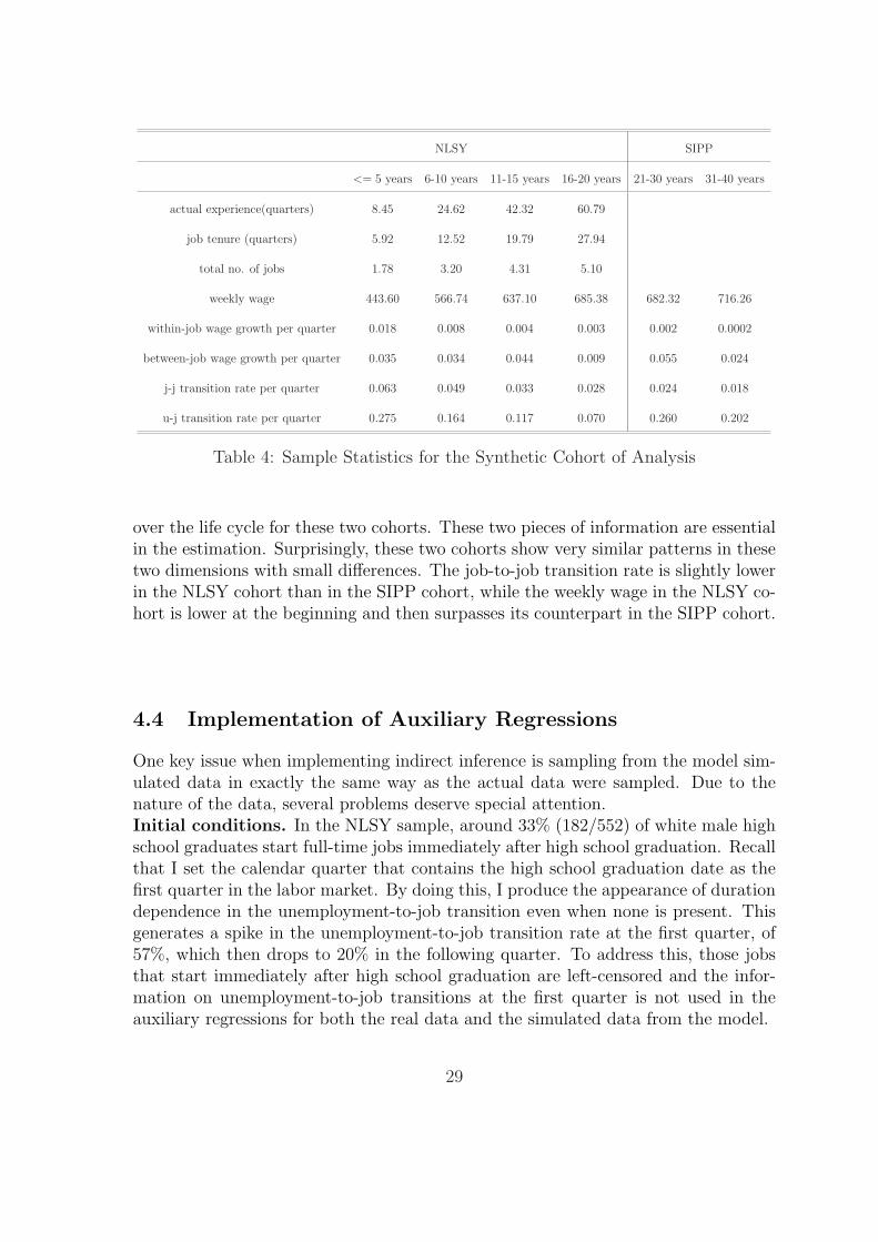
Table 4 shows some main sample statistics for the synthetic cohort of analysis.Columns 2 to 5 show statistics for the NLSY cohort and columns 6 and 7 for theSIPP cohort. Full-time work experience increases from 8.5 quarters over the first 5years to 61 quarters if one has been in the labor market for 16 to 20 years. Jobseniority increases from around 6 quarter (1.5 years) over the first 5 years to around28 quarters (7 years) if one has been in the market for 16 to 20 years. As experienceand job seniority increase, the average weekly wage increases from $443 to $685 overthe same period of time. The wage grows at a decreasing rate. From year 5 to year10, the wage increases by more than $120, then $70 from years 10 to 15 and $50 fromyears 15 to 20. No wage growth is seen from year 20 to year 30 and only a slightincrease, about $34, from year 30 to year 40. On average, a high school graduate canexpect wage growth of 2% per quarter on the job over the first 5 years. This amountsto about 8% per year. This growth declines over time, down to 0.3% per quarter ifone has been in the market for 16 to 20 years. Job switching results in wage growthof 3.5% per quarter over the first 5 years, which is almost twice as high as the growthon the job over the same period of time. The between-job wage growth does notdecrease as much as the within-job wage growth, at 2.4% per quarter over the last 10years. The job-to-job transition rate decreases over time and as the wage increases,from 6% per quarter over the first 5 years to about 2% over the last 10 years. Theunemployment-to-job transition rate also decreases over time from 27.5% per quarterover the first 5 years in the labor market to 7% if one has been in the market for 16to 20 years. The unemployment-to-job transition rate in the SIPP cohort is relativelyhigher than and does not decrease as much as that in the NLSY cohort.

One potential problem with using a synthetic cohort is that of cohort and timeeffects. The estimation and analysis based on the synthetic cohort would be inappro-priate if the NLSY cohort and the SIPP cohort were too different. To see how differentthese two cohorts are, Figure 9 plots the job-to-job transition rates and weekly wages

28

NLSY SIPP

<= 5 years 6-10 years 11-15 years 16-20 years 21-30 years 31-40 years

actual experience(quarters) 8.45 24.62 42.32 60.79

job tenure (quarters) 5.92 12.52 19.79 27.94

total no. of jobs 1.78 3.20 4.31 5.10

weekly wage 443.60 566.74 637.10 685.38 682.32 716.26

within-job wage growth per quarter 0.018 0.008 0.004 0.003 0.002 0.0002

between-job wage growth per quarter 0.035 0.034 0.044 0.009 0.055 0.024

j-j transition rate per quarter 0.063 0.049 0.033 0.028 0.024 0.018

u-j transition rate per quarter 0.275 0.164 0.117 0.070 0.260 0.202

Table 4: Sample Statistics for the Synthetic Cohort of Analysis

over the life cycle for these two cohorts. These two pieces of information are essentialin the estimation. Surprisingly, these two cohorts show very similar patterns in thesetwo dimensions with small differences. The job-to-job transition rate is slightly lowerin the NLSY cohort than in the SIPP cohort, while the weekly wage in the NLSY co-hort is lower at the beginning and then surpasses its counterpart in the SIPP cohort.

4.4 Implementation of Auxiliary Regressions

One key issue when implementing indirect inference is sampling from the model sim-ulated data in exactly the same way as the actual data were sampled. Due to thenature of the data, several problems deserve special attention.Initial conditions. In the NLSY sample, around 33% (182/552) of white male highschool graduates start full-time jobs immediately after high school graduation. Recallthat I set the calendar quarter that contains the high school graduation date as thefirst quarter in the labor market. By doing this, I produce the appearance of durationdependence in the unemployment-to-job transition even when none is present. Thisgenerates a spike in the unemployment-to-job transition rate at the first quarter, of57%, which then drops to 20% in the following quarter. To address this, those jobsthat start immediately after high school graduation are left-censored and the infor-mation on unemployment-to-job transitions at the first quarter is not used in theauxiliary regressions for both the real data and the simulated data from the model.

29

0.0

5.1

.15

fraction

0 20 40 60 80 100 120 140 160quarter

NLSY Fitted valuesSIPP Fitted values

(a) job-to-job transition rates

400

500

600

700

800

mean w

eekly

wage

0 20 40 60 80 100 120 140 160quarter

NLSY Fitted valuesSIPP Fitted values

(b) weekly wages

Figure 9: Comparisons of the NLSY Cohort and the SIPP Cohort

30

Wages in the NLSY. In the NLSY, during each interview, respondents are askeda wage for each job held since the last interview. If a job is ongoing at the interviewweek, the reported wage is treated as the wage as of the interview week for that job.If a job ends before the interview week, the reported wage is treated as the wage as ofthe last week for that job. Meanwhile, respondents are interviewed once a year before1994 and once every two years after 1994. Hence wages are not available for everyquarter, only for those quarters that contain the interview weeks and the last weeksof jobs. This poses two issues when implementing the auxiliary regressions, selectionand timing of the wages. The inclusion of wage as a regressor in equations (9) and(13) leads to a selection problem. This is because wages are only observed duringquarters that contain the last weeks of jobs and the interview weeks. Hence the prob-ability of a job-to-job transition is higher for those quarters with wage observationsthan that for every quarter. In fact, the mean job-to-job transition probability for allquarters is around 4% per quarter and the mean job-to-job transition probability ismuch higher around 17% for those quarters with wage observations. To address this,I exclude wages from regressions (9) and (13) for both the data and the model.

The other selection problem occurs for the initial wage regression in the NLSY,regression (12). Recall that I only select those high school graduates who graduatedbetween 1978 and 1984. Most of the interviews from 1978 to 1984 happen from Jan-uary to July, which are in the first and second calendar quarter. The most commoncalendar quarter for high school graduation is the second (April-June). Recall againthat I set the calendar quarter that contains high school graduation date as the firstquarter in the labor market. Therefore, the first job most likely starts from the thirdcalendar quarter, if any, which is not the interview quarter. Therefore, in order tohave a wage observation for the first job at the third calendar quarter, the job hasto be short to get a stopping wage at next interview. This results in a selection ofshort jobs conditional on having wage observations. In fact, the average duration ofthe first jobs in the NLSY sample is 13.4 quarters while the counterpart for first jobsconditional on having a wage in quarter 2 is only 1.6 quarters. The estimates of thedistribution of the rental rate are likely downward biased if only the wages of theseshort jobs are used since short jobs usually have low wages. To address this, I use thefirst available wage within the first year in the labor market from the first jobs in theauxiliary regression for the NLSY sample. By doing this, I ignore the wage growthover the first year on the first job and hence may bias the human capital investmentdownward at the beginning.

The wage timing problem occurs because in the NLSY wages are not available forevery quarter. Meanwhile, interviews are conducted roughly once a year before 1994and every two years after 1994. In the NLSY sample, the average distance betweentwo quarters that have wage observations on the same job is about 4 quarters before1994 and about 7.4 quarters after 1994. To make the model consistent with the datawhen implementing indirect inference, I apply an interviewing scheme to the simu-lated data where interviews start from quarter 2 and run for every 4 quarters before

31

quarter 58, and every 8 quarters after that. The quarter 58 corresponds to the yearof 1994 in the NLSY. I use only those wages that fall in the interview quarters andstopping quarters of jobs for the simulated data when estimating regressions (10) and(11). In addition to this, the log wage growth in regression (10) is transformed intoquarterly log wage growth by dividing the wage growth by the tenure differences inboth the real data and the simulated data.

Wages of older workers in the SIPP. Recall that the rental rate equivalentfor the unemployed, b, is identified through the minimum wage among those post-displaced workers at the last period. However, due to the short panel of the SIPPand the retirement of most older workers, there are too few post-displaced wage ob-servations. Using these few observations could bias the estimate of b. Hence insteadof using only the post-displaced wages at the last period, I use all the wages at thelast period. For this version of the paper, I calibrate b to 1.2, which is derived bydividing $120, the minimum wage in the last period in the SIPP, by 100, the initialhuman capital, rather than estimate it through the indirect inference.

5 Preliminary Results

A set of preliminary parameter estimates are presented in Table 5.15 The estimateof the search efficiency parameter, λ, is 0.056, which means that the job offer arrivalprobability for one unit of search effort is 5.6% per quarter. This estimate is smallerthan those found by the search literature that also endogenizes search intensity. Lise(2005) finds that λ is 0.65 per quarter using the NLSY. Christensen et al. (2005) usingDanish data find that λ is about 0.14 per quarter. The estimate for the search cost,γ is around 20. This is much higher than that in Christensen et al. (2005), around2. The estimate for the learning ability parameter in the human capital productionfunction is around 0.5, which is higher than those in the human capital literature.For example, Heckman et al. (1998) find that a is around 0.08. However, a is relatedto the initial human capital level. The initial human capital in my paper is almost 10times bigger than that in their paper. Thus a needs to be bigger in order to generatethe same amount of human capital investment.16 The curvature parameter, α, in thehuman capital production function is 0.14 and is smaller than that in Heckman et al.(1998), around 0.8. Partly this is because their analysis is based on annual wageswhile in my paper I assume human capital production takes place every quarter. Themean of the log of the rental rate distribution is 1.3 and the standard deviation is 0.3.

15Standard errors of these estimates are not available for this version.16Human capital investment is a decreasing function of human capital stock. If a were the same as

in their paper, my model would generate less human capital investment. Thus, the estimate of a inmy paper is larger than that in their paper in order to generate the same amount of the investment.

32

parameter estimate

search efficiency λ 0.056

search cost curvature γ 19.530

learning ability a 0.513

curvature in human capital production function α 0.144

mean of rental rate distribution µ 1.311

s.d. of the rental rate distribution σ 0.329

initial human capital h0 100

job destruction δ 0.03

rental rate equivalency for the unemployed b 1.2

Table 5: Preliminary Parameter Estimates

This translates into a mean rental rate of 3.9 and with a standard deviation of 1.3.Thus for one unit of human capital, the mean rental rate is about $3.90 per week.The implied rental rate distribution, as plotted in panel (b) of Figure 11, is disperse,ranging from 1 to 10, and skewed to the right with a long right tail. Compared to therental rate distribution, b is almost at the low end. Hence the rental rate distributionis fully uncovered. The parameters b is calibrated to match the minimum wage atthe last period in the SIPP. The minimum wage generated by the model based onthese estimates at the last period is about $127, which is quite close to the empiricalcounterpart in the SIPP, $120.

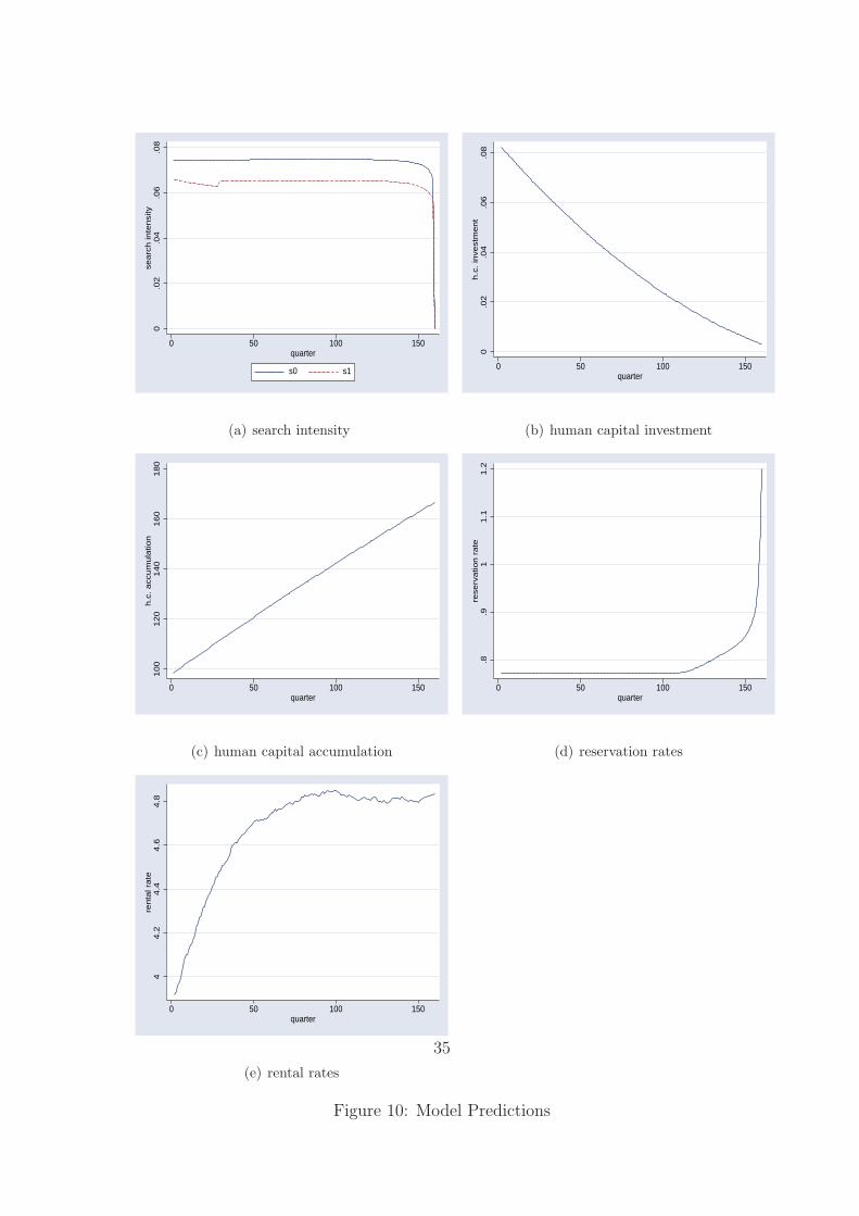
Under these estimates, the model predicts that human capital investment is de-creasing over time and leads an average increase in human capital over the life cycleof 65%, as shown in panels (b) and (c) of Figure 10. Panel (a) in Figure 11 plots thekernel density for the distribution of human capital at the end of the life cycle. Wecan see that the distribution is very disperse, ranging from 100 to 200. In the model,workers start with the same amount of human capital. However they experience verydifferent labor market trajectories over the life cycle resulting in different paths ofhuman capital investment and search behavior. These two forces working togethermake even ex-ante identical workers very different at the end of the life cycle. Withregard to search, the model predicts that the job arrival rate for the unemployed

33

workers is higher than that on the job, as shown in panel (a) of Figure 10. This isconsistent with most findings in the search literature. The reservation rate, plottedin panel (d) of Figure 10, is increasing over time and equal to the lowest rental rate inthe distribution at the beginning of the life cycle to take advantage of human capitalinvestment. The average rental rate, plotted in panel (e) of Figure 10, increases overtime from an average of 3.9 initially to 4.8 at the end of the life cycle. Panel (c) inFigure 11 plots two wage distributions, one for wages at the beginning of the life cycleand the other at the end of the life cycle. At the beginning of the life cycle, workershave the same amount of human capital, they are willing to accept any rental rate tostart accumulating human capital. Hence the initial wage distribution centers aroundthe mean of the rental rate multiplied by the initial human capital. The wage dis-persion at the beginning comes from the dispersion of the rental rate and associatedvariation in human capital investment. The wage distribution at the end of life cycleshifts to the right and is much more dispersed than the initial wage distribution. Thisis because both the rental rate and human capital grow over time. The dispersionnot only comes from the dispersion in the rental rates but also from that in humancapital levels at the end of the life cycle.

To examine the interactions between human capital accumulation and job search,I conduct two counterfactual experiments. In the first experiment, I turn off search onthe job but allow for exogenous unemployment-to-job transitions and job destruction.Everyone at the beginning of the life cycle takes a random draw from the rental ratedistribution and keeps it until the end of the life cycle. Compared to the model thathas both human capital accumulation and job search, this situation yields a loweraverage investment in human capital at the beginning of the life cycle and higher av-erage investment in the middle, as shown in panel (a) of Figure 12. At the beginningof the life cycle, workers in these two models start with the same amount of humancapital and the same rental rate. However, workers in the model with on-the-jobsearch expect their rental rates to rise over the life cycle and thus invest more at thebeginning. In contrast, workers in the model without on-the-job search know theirrental rates will stay the same and therefore their human capital investment decisionis independent of their rental rates. Over time, workers in the model with job searchhave higher rental rates than their counterparts in the model without job search thusreducing the investment. Overall, workers in these two models accumulate almost thesame amount of human capital on average over the life cycle. However, there is nodispersion in human capital in the model without on-the-job search.

In the second experiment, I turn off human capital accumulation and only allowfor job search. Compared to the model with human capital accumulation, workers inthe search only model search less intensively while unemployed and raise their reser-vation rates, as plotted in panels (c) and (e) of Figure 12. Search intensity on the jobis also lower than with human capital accumulation, as shown in panel (d) of Figure12. Panel (f) in Figure 12 plots life cycle wage profiles for 3 scenarios: model withboth human capital accumulation and job search, model with human capital accumu-

34

0.0

2.0

4.0

6.0

8se

arc

h in

tensi

ty

0 50 100 150quarter

s0 s1

(a) search intensity

0.0

2.0

4.0

6.0

8h.c

. in

vest

ment

0 50 100 150quarter

(b) human capital investment

100

120

140

160

180

h.c

. acc

um

ula

tion

0 50 100 150quarter

(c) human capital accumulation

.8.9

11.1

1.2

rese

rvatio

n r

ate

0 50 100 150quarter

(d) reservation rates

44.2

4.4

4.6

4.8

renta

l rate

0 50 100 150quarter

(e) rental rates

Figure 10: Model Predictions

35

0.0

1.0

2.0

3D

ensi

ty

100 120 140 160 180 200h

(a) distribution of h

0.1

.2.3

Densi

ty0 2 4 6 8 10

r

(b) distribution of rental rate

0.0

01

.002

.003

.004

densi

ty

0 500 1000 1500 2000wage

density: wage at the beginning density: wage at the end

(c) wage distributions

Figure 11: Distributions of Human Capital, Rental Rates, and Wages

36

lation only, and model with search only. As we can see, the average wage increasesby $440 over the life cycle in the model with both human capital accumulation andjob search. The model with human capital accumulation generates a wage increaseof $295. The model with job search can only generate a wage increase of $90. Thus,human capital accumulation is more important and accounts for 67-80% of the totalwage growth and job search accounts for 20-33%.

Tables 6 to 8 compare the auxiliary parameters from the data and the model. Themodel does a fairly good job in predicting the correct signs for most of the auxiliaryparameters. In particular, the model does well in matching the job-to-job transitionsfor the older workers, as shown in column 9 of Table 6, the initial job-to-job tran-sitions, as shown in column 7 of Table 6, and the total wage growth, as shown incolumn 3 of Table 7. However, the model also has some difficulties matching the datain other dimensions.

First, the model under-predicts the unemployment-to job transitions and job-to-job transitions, as shown in Table 6 and panels (b) and (c) in Figure 13. Partly thismay be because the wage information is not used in the auxiliary regressions relatedto job-to-job transitions. Wage information is an important piece of identificationinformation for the search parameters. However, due to the selection problem dis-cussed in the previous section, wages are excluded from the regressions. This maycause the model to have difficulty in pinning down the right search parameters. Apossible solution is to impute the wage for each quarter in the NLSY and in themodel. This way the selection problem can be avoided and more variation can beintroduced into the regressions by including the wage as a regressor. Another pos-sible reason for the poor fit is that the model has only one search cost function forboth unemployed and employed workers. This may make it difficult for the model tomatch both unemployment-to-job transitions and job-to-job transitions. To matchthe relatively low transitions on the job in the data, the model imposes a low λ anda high γ. However, at the same time, this generates low unemployment-to-job tran-sitions. There are more observations in the data on job-to-job transitions than onunemployment-to-job transitions. This puts more weight on the job-to-job transitionsin the weighting matrix, making that a priority to match. Hence under-prediction ofunemployment-to-job transition results.

Second, the model does not generate as much curvature for wage growth as in thedata, as seen in panel (a) of Figure 13. The estimate of the curvature parameter inthe human capital production function is smaller than those in the human capitalliterature. Partly this is because the model under-predicts the job-to-job transitions.Thus in order to match the overall wage growth in the data, the curvature in thehuman capital production function has to be smaller and the ability parameter a hasto be bigger to induce substantial wage growth due to human capital accumulation.

37

0.0

2.0

4.0

6.0

8h.c

. in

vest

ment

0 50 100 150quarter

both no search

(a) human capital investment

100

120

140

160

180

h.c

. acc

um

ula

tion

0 50 100 150quarter

both no search

(b) human capital accumulation

0.0

2.0

4.0

6.0

8ls

0

0 50 100 150quarter

both no h accumulation

(c) search intensity for the unemployed

0.0

2.0

4.0

6.0

8ls

1

0 50 100 150quarter

both no h accumulation

(d) search intensity on the job

.8.9

11.1

1.2

rese

rvatio

n r

ate

0 50 100 150quarter

both no h accumulation

(e) reservation rates

300

400

500

600

700

800

wage

0 50 100 150quarter

both no searchno h accumulation

(f) wages

Figure 12: Counterfactual Experiments

38

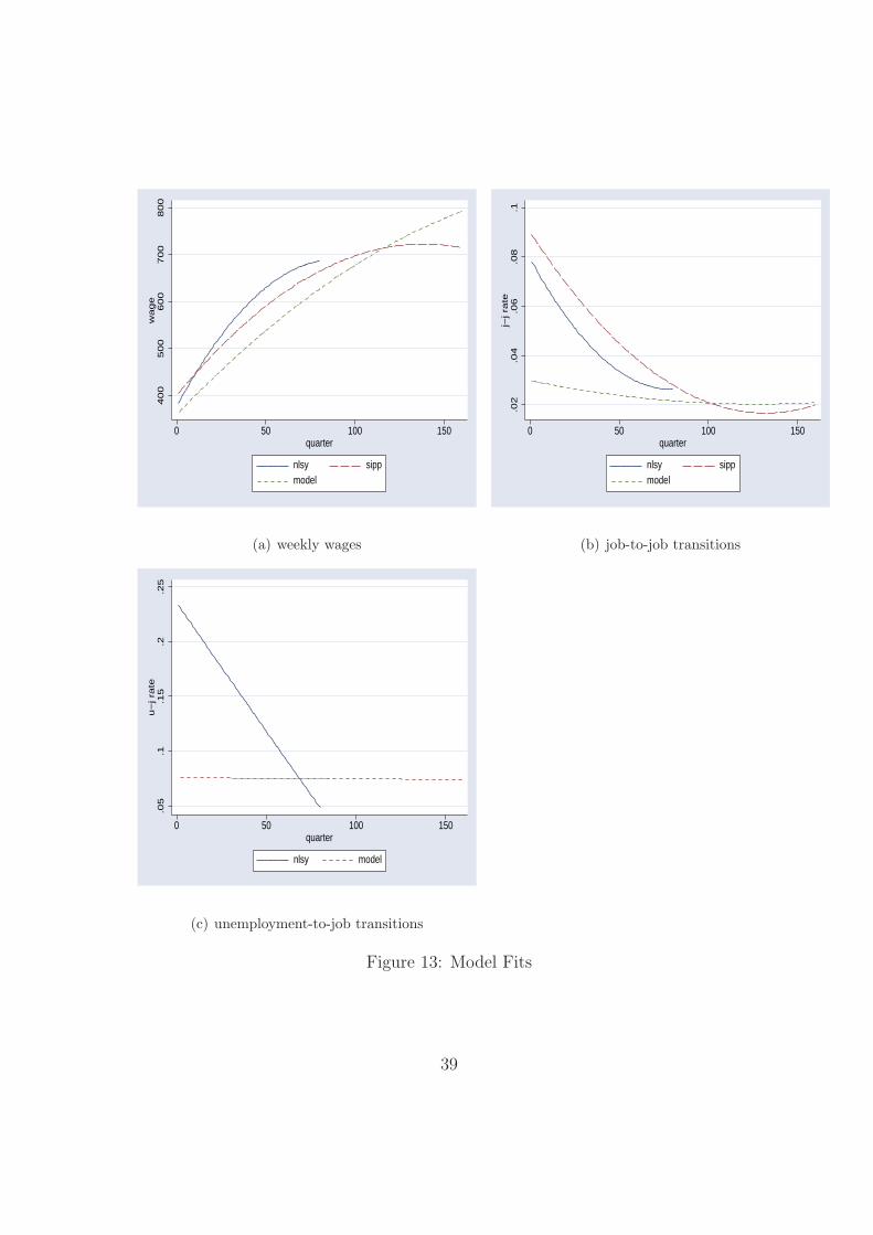
400

500

600

700

800

wage

0 50 100 150quarter

nlsy sippmodel

(a) weekly wages

.02

.04

.06

.08

.1j−

j ra

te

0 50 100 150quarter

nlsy sippmodel

(b) job-to-job transitions

.05

.1.1

5.2

.25

u−

j ra

te

0 50 100 150quarter

nlsy model

(c) unemployment-to-job transitions

Figure 13: Model Fits

39

u-to-j transition j-to-j transition

NLSY Model NLSY Model NLSY Model SIPP Model

(<= quarter 80) (<= quarter 80) (quarter 2) ( quarters 81-160)

exp/100 -0.251 0.003 -0.048 -0.045 -0.019 0.014

exp2/10000 0.266 -0.015 0.032 0.044

tenure/100 -0.250 -0.027 -1.031 -0.712

tenure2/10000 0.273 0.019 0.97 1.067

w/100 -0.011 -0.019

w2/10000 0.001 0.001

cons 0.180 0.074 0.081 0.036 0.165 0.093 0.089 0.098

Note: number in bold are statistically significant from zero.

Table 6: Auxiliary Parameters from the Data and the Model-Transition Regressions

log wage

NLSY Model NLSY Model SIPP Model

(<= quarter 80) (quarter 2) (quarters 81-160 )

exp/100 1.309 0.975 -0.703 0.769

exp2/10000 -1.032 -0.494 0.345 -0.184

tenure/100 0.940 0.498 0.054 1.509

tenure2/10000 -0.751 -0.013 0.134 -1.660

dju/100 10.132 22.247

cons 5.834 5.790 5.862 5.642 6.773 5.874

Note: number in bold are statistically significant from zero.

Table 7: Auxiliary Parameters from the Data and the Model-Wage Regressions

40

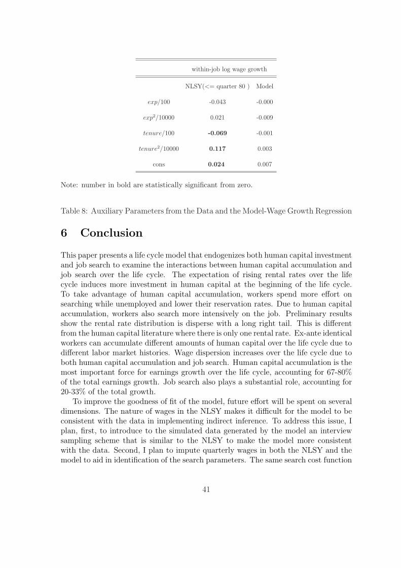
within-job log wage growth

NLSY(<= quarter 80 ) Model

exp/100 -0.043 -0.000

exp2/10000 0.021 -0.009

tenure/100 -0.069 -0.001

tenure2/10000 0.117 0.003

cons 0.024 0.007

Note: number in bold are statistically significant from zero.

Table 8: Auxiliary Parameters from the Data and the Model-Wage Growth Regression

6 Conclusion

This paper presents a life cycle model that endogenizes both human capital investmentand job search to examine the interactions between human capital accumulation andjob search over the life cycle. The expectation of rising rental rates over the lifecycle induces more investment in human capital at the beginning of the life cycle.To take advantage of human capital accumulation, workers spend more effort onsearching while unemployed and lower their reservation rates. Due to human capitalaccumulation, workers also search more intensively on the job. Preliminary resultsshow the rental rate distribution is disperse with a long right tail. This is differentfrom the human capital literature where there is only one rental rate. Ex-ante identicalworkers can accumulate different amounts of human capital over the life cycle due todifferent labor market histories. Wage dispersion increases over the life cycle due toboth human capital accumulation and job search. Human capital accumulation is themost important force for earnings growth over the life cycle, accounting for 67-80%of the total earnings growth. Job search also plays a substantial role, accounting for20-33% of the total growth.

To improve the goodness of fit of the model, future effort will be spent on severaldimensions. The nature of wages in the NLSY makes it difficult for the model to beconsistent with the data in implementing indirect inference. To address this issue, Iplan, first, to introduce to the simulated data generated by the model an interviewsampling scheme that is similar to the NLSY to make the model more consistentwith the data. Second, I plan to impute quarterly wages in both the NLSY and themodel to aid in identification of the search parameters. The same search cost function

41

for both unemployed and employed workers may make it difficult for the model tomatch both unemployment-to-job transitions and job-to-job transitions. To addressthis, I plan to introduce heterogeneity in terms of search technology or human capitalproduction to improve the flexibility of the model.

42

References

Bagger, J., F. Fontaine, F. Postel-Vinay, and J.-M. Robin (2007). A tractable equi-librium search model of individual wage dynamics with experience accumulation.Mimeo.

Barlevy, G. (2005). Estimating models of on-the-job search using record statistics.Federal Reserve Bank of Chicago Working Paper.

Ben-Porath, Y. (1967). The production of human capital and the life cycle earnings.Journal of Political Economy 75 (4), 352–365.

Benhabib, J. and C. Bull (1983). Job search: the choice of intensity. Journal ofPolitical Economy 91 (5), 747–764.

Bowlus, A. J., N. M. Kiefer, and G. R. Neumann (2001). Equilibrium search modelsand the transition from school to work. International Economics Review 42 (2),317–343.

Brown, C. (1976). A model of optimal human-capital accumulation and the wages ofyoung high school graduates. Journal of Political Economy , 299–316.

Bunzel, H., B. Christensen, P. Jensen, N. Kiefer, L. Korsholm, L. Muus, G. Neumann,and M. Rosholm (1999). Investment in human capital versus differences in companyproductivity levels: Specification and estimation of equilibrium search models fordenmark. Mimeo.

Burdett, K. and D. T. Mortensen (1998). Wage differentials, employer size, andunemployment. International Economic Review 39, 257–273.

Christensen, B., a. D. M. R. Lentz, G. Neumann, and A. Werwatz (2005). On-the-jobsearch and the wage distribution. Journal of Labor Economics 23 (1), 31–57.

Dustmann, C. and C. Meghir (2005). Wages, experience, and seniority. Review ofEconomic Studies 72, 77–108.

Eckstein, Z. and K. Wolpin (1995). Duration to first job and the return to schooling:estimates from a search-matching model. Review of Economic Studies 62 (2), 263–286.

Goffe, W., G. Ferrier, and J. Rogers (1994). Global optimization of statistical func-tions with simulated annealing. Journal of Econometrics 18, 115–168.

Gourieroux, C., A. Monfort, and E. Renault (1993). Indirect inference. Journal ofApplied Econometrics 8, S85–S118.

43

Heckman, J. (1976). A life-cycle model of earnings, learning, and consumption. Jour-nal of Political Economy 84 (2), S11–S44.

Heckman, J., L. Lochner, and C. Taber (1998). Explaining rising wage inequality:Explorations with a dynamic general equilibrium model of labor earnings withheterogeneous agents. Review of Economics Dynamics 1 (58).

Hugget, M., G. Ventura, and A. Yaron (2004). Human capital and earnings distribu-tion dynamics. Georgetown University, Mimeo.

Jovanovic, B. (1979). Firm specific capital and turnover. Journal of Political Econ-omy 87, 1246–1260.

Lise, J. (2005). On-the-job search and precautionary savings: Theory and empiricsof earnings and wealth inequality. Queen’s University, Mimeo.

Mincer, J. and B. Jovanovic (1979). Labor mobilty and wages. NBER Working Paper357.

Mortensen, D. (2003). Wage Dispersion: Why Are Similar Workers Paid Differently?Cambridge, Massachusetts: MIT Press.

Omer, V. (2004). Wage growth, search and experience: Theory and evidence. Uni-versity of Minnesota, Mimeo.

Pavan, R. (2007). Individual wage dynamics and heterogeneity in search technology.University of Rochester, Mimeo.

Postel-Vinay, F. and J.-M. Robin (2002). Equilibrium wage dispersion with workerand employer heterogeneity. Econometrica 70 (6), 2295–2350.

Rendon, S. (2006). Job search and asset accumulation under borrowing constraints.International Economic Review 47 (1), 233–263.

Rubinstein, Y. and Y. Weiss (2005). Post schooling wage growth: Investment, searchand learning. Tel-Aviv University, Mimeo.

Schonberg, U. (2005). Wage growth due to human capital accumulation and jobsearch: A comparision between the united states and germany. University ofRochester, Mimeo.

Seater, J. (1977). A unified model of consumption, labor supply, and job search.Journal of Economic Theory 14, 349–372.

Shimer, R. (2004). Search intensity. University of Chicago, Mimeo.

Topel, R. and M. Ward (1992). Job mobility and careers of young men. QuarterlyJournal of Economics 107 (2), 439–479.

44

Wolpin, K. (1992). The determinants of black-white differences in early employmentcareers: search, layoffs, quits, and endogenous wage growth. Journal of PoliticalEconomy 100, 535–560.

Yamaguchi, S. (2006). Job search, bargaining, and wage dynamics. McMaster Uni-versity, Mimeo.

45