CloudSat Project A NASA Earth System Science Pathfinder Mission

Level 2 GEOPROF Product Process Description and Interface Control Document Product: 2B-GEOPROF Product Version: P1_R05 Document Revision: 0 Date: 18 June 2018 Address questions concerning the document to: Roger Marchand rojmarch@u.washington.edu or Gerald Mace mace@met.utah.edu (801) 585-9489

2

Document Revision History Date Revision Description Section(s) Affected 18 April 2017 0 Initial Release All

3

Contents

Contents......................................................................................................................................31. Introduction................................................................................................................................42. AlgorithmTheoreticalBasis(Overview)..........................................................................53. AlgorithmInputs.......................................................................................................................63.1CloudSat.......................................................................................................................................................63.1.1CloudSatLevel1BCPR...................................................................................................................................63.1.2CloudSatLevel1AAuxiliaryData..............................................................................................................6

3.2AuxiliaryDatasets(Non-CloudSat)..................................................................................................73.2.1MODIScloudmaskdata(MODIS-AUX)...................................................................................................73.2.2ECMWF(ECMWF-AUX)..................................................................................................................................7

4. AlgorithmSummary.................................................................................................................84.1TheCloud/HydrometeorMask........................................................................................................84.1.1SignificantEchoMaskAlgorithm...............................................................................................................84.1.2SurfaceClutterIdentification...................................................................................................................11

4.2VariablesrelatedtotheMODISCloudMask.............................................................................125. DataProductOutputFormat..............................................................................................185.1FormatOverview..................................................................................................................................185.2CPRLevel2GEOPROFHDF-EOSDataContents......................................................................18

6. Summaryofchangesfrompreviousversions..............................................................207. References................................................................................................................................228. AcronymList............................................................................................................................239. AppendixA.FlowchartsofMODISpixelcloudinesscharacterizations................24

4

1. Introduction The presence or absence and vertical location of cloud layers impose powerful constraints on the radiative properties of an atmospheric column and, thereby, modulate strongly the radiative heating rate of the column. Information on the vertical distribution of cloud layers from analyses of conventional passive-sensor satellite radiometers (that observe only the emitted and reflected radiance from the atmosphere and surface) is limited and can provide only a rough estimate for the location and vertical extent of clouds and precipitation. Active remote sensors such as CloudSat, on the other hand, are uniquely adapted to observe the vertical location of hydrometeor layers. Therefore, a basic requirement of the CloudSat project is to use data from the Cloud Profiling Radar (CPR) to identify those levels in the vertical column sampled by CloudSat that contain significant radar echo from hydrometeors and to produce an estimate of the radar reflectivity factor for each volume deemed to contain significant echo (Stephens et al, 2001). The CloudSat orbit follows closely the orbit of the EOS PM1 satellite (Aqua) from which a number of advanced passive remote sensors observe the earth. This synergistic association can add significantly to our understanding of the CloudSat geometrical profile and we use this data source to our advantage. In particular, the Moderate-Resolution Imaging Spectroradiometer (MODIS) provides information regarding the occurrence and horizontal distribution of clouds within the CloudSat footprint. The MODIS cloud mask product (Ackerman et al., 1998) is available for use in the operational CloudSat processing stream. The MODIS cloud mask contains not only an estimate of the likelihood of clouds in 1km MODIS pixels, but also contains the results of a number tests with MODIS-observed spectral radiances that provide limited information on the nature of the clouds in the vertical column. The GeoProf dataset (whose algorithms are described in this documents) summarizes and stores some MODIS spectral tests results in order to assist in comparisons of the CloudSat hydrometeor mask and MODIS cloud mask. This document describes the algorithms that have been implemented operationally to identify significant radar echo in the CloudSat data stream and to summarize associated MODIS cloud detections. Specifically, the objective of the resulting GeoProf data are to:

• Determine if the radar data for each radar resolution volume is significantly different from radar measurement noise or surface clutter and, thus, deemed to contain hydrometeors (that is clouds or precipitating particles),

• Quantify the likelihood that a given range resolution volume with characteristics different from noise actually contains hydrometeors,

• Place the radar observations on a fixed vertical grid, relative to mean sea level, and

• Summarize information from the MODIS cloud mask associated with each CloudSat echo profile.

5

* Significant changes to the current release (P1 R05) of the CloudSat product from the previous release (R04) are:

• Reduced false detection rate • Improved estimates of radar noise floor power • Re-optimized filter parameters for “weak” detections (esp. confidence flag <= 10) • Improved surface clutter identification • Addition of an along track (profile-by-profile) estimate of the radar Minimum

Detectable Signal (MDS). • Improved DEM and Quality Flags (from 1B-CPR-R05)

We note the original release of R05 products (known as P0 R05) had a bug in the code used to determine the noise floor power. This bug created many problems and increases number of false detections. While the impact is minor for data prior to the 2011 Battery Anomaly (that is data files from epoch E02 to E04 provided in the file names), we recommend discarding all P0 R05 data and using only the most recent data (file names contain P1 R05).

2. Algorithm Theoretical Basis (Overview) The Geometrical Profile (GeoProf) algorithm contains two parts. The first part identifies significant radar echo in profiles of returned radar power from the CloudSat CPR data and is described in section 4.1. The second part is designed to assists in comparisons of the geometrical profile algorithm with the MODIS cloud mask spectral tests, section 4.2. The CloudSat hydrometeor detection algorithm is similar to the algorithm developed by Clothiaux et al. [1995, 2000] for vertically pointing cloud radar, but with two significant changes. These changes are (1) a power probability-weighting scheme and (2) an along-track integration scheme. The along-track integration scheme helps identify targets that are too weak to be detected at full resolution (0.16s) but which can be detected through along-track (temporal) averaging of the data. The algorithm used in R05 is the same as used in R04, with a few minor changes. The R04 algorithm is documented in detail in Marchand et al. [2008] and summarized below in section 4.1.1. Changes to this algorithm since R04 are highlighted in the text. In addition, the CloudSat product contains a clutter identification algorithm, which is necessitated by the occurrence of additional scattering from the Earth surface contributing to return power measurements near the surface. The R05 surface clutter identification is significantly changed and improved from R04 and is described 4.1.2. This algorithm (and updates discussed in section 4.1.1) will likewise be documented in the peer-reviewed literature in the near future [Marchand et al. 2018]. Unlike typical weather radars, which operate at much longer wavelengths and are primarily designed to detect rain rather than clouds, the effect of water vapor on CloudSat observed reflectivity can be significant. Two-way attenuation from the surface to the satellite of more than 5 dBZ is not unusual in the tropics. The GeoProf dataset contains

6

an estimate of the attenuation due to gasses (primarily water vapor but also including the effect of oxygen). This estimate is based on the Liebe 87 model and water vapor amounts from ECMWF analysis. We STRESS the “reflectivity” field in the GeoProf product is the measured reflectivity (return power) and has not been compensated for any attenuation. Users are advised to correct the measured power, if such is needed for their application. Note that hydrometeors themselves can also cause significant attenuation and multiple scattering. NO estimates for the attenuation from hydrometeors or multiple scattering contributions are provided. The attenuation due to hydrometeors depends strongly on the phase of the condensate and the particle size (distribution) and cannot be determined accurately from the radar reflectivity alone.

3. Algorithm Inputs 3.1 CloudSat 3.1.1 CloudSat Level 1B CPR The CPR Level 1 B (Li and Durden, 2001) is the main input for the GEOPROF Algorithm. 2B-GEOPROF algorithm requires the following inputs from the Level 1B CPR Science Data are (see Level 1B CPR Process Description and Interface Control Document). Spacecraft latitude and longitude are used to locate the position of satellite. Range bin sizes, Range to first bin, and Surface bin number are used to locate the height of resolution volumes. Received echo power is used as input to the cloud mask algorithm and for calculation of radar reflectivity. Radar transmission power, wavelength, and radar calibration coefficients are also needed when calculating radar reflectivity.

- Spacecraft latitude - Spacecraft longitude - Spacecraft altitude - Range bin sizes - Range to first bin - Surface bin number (based on radar return) - Wavelength - CPR radar calibration coefficients - Radar transmission power - Received echo power - Number of pulses transmitted - Surface clutter index and estimated surface clutter

3.1.2 CloudSat Level 1A Auxiliary Data Level 2 GEOPROF processing requires the following data:

− Land/Sea Flag − Altitude of Surface

7

3.2 Auxiliary Datasets (Non-CloudSat) 3.2.1 MODIS cloud mask data (MODIS-AUX) The MODIS cloud mask data, used here for the comparison of the geometrical profile algorithm with the MODIS cloud mask spectral tests.

− MODIS latitude − MODIS longitude − 48-bit MODIS mask data in a swath along the CLOUDSAT ground track

3.2.2 ECMWF (ECMWF-AUX) Meteorological data interpolated temporally and spatially to the CLOUDSAT range resolution volumes are needed to aid in the comparison of MODIS mask data with CLOUDSAT profile data. Temperature and pressure profiles are required for the calculation of CPR echo top characterization (see Table 4) and to estimate gasses attenuation.

− Temperature profile − Atmosphere pressure profile − Atmosphere water vapor

8

4. Algorithm Summary 4.1 The Cloud / Hydrometeor Mask 4.1.1 Significant Echo Mask Algorithm The primary GeoProf output is a “Cloud Mask” which indicates which radar reflectivity measurements are likely due to real hydrometeors (that is clouds or precipitating particles) and which are likely measurement noise or likely contain a significant contribution from surface clutter. The mask contains an integer values ranging from 0 to 40 (as specified in the table #1, below) indicating the likelihood that a given radar resolution volume reflectivity represents a good measurement.

Mask Value

Meaning % False Detections Goals for R05

-9 Bad or missing radar data 5 Significant return power but likely surface clutter

6-10 Very weak echo (detected using along-track averaging)

< 16 %

20 Weak echo (detection may be artifact of spatial correlation)

< 16%

30 Good echo < 2 % 40 Strong echo < 0.2 %

Table #1 – GeoProf R05 Cloud Mask values.

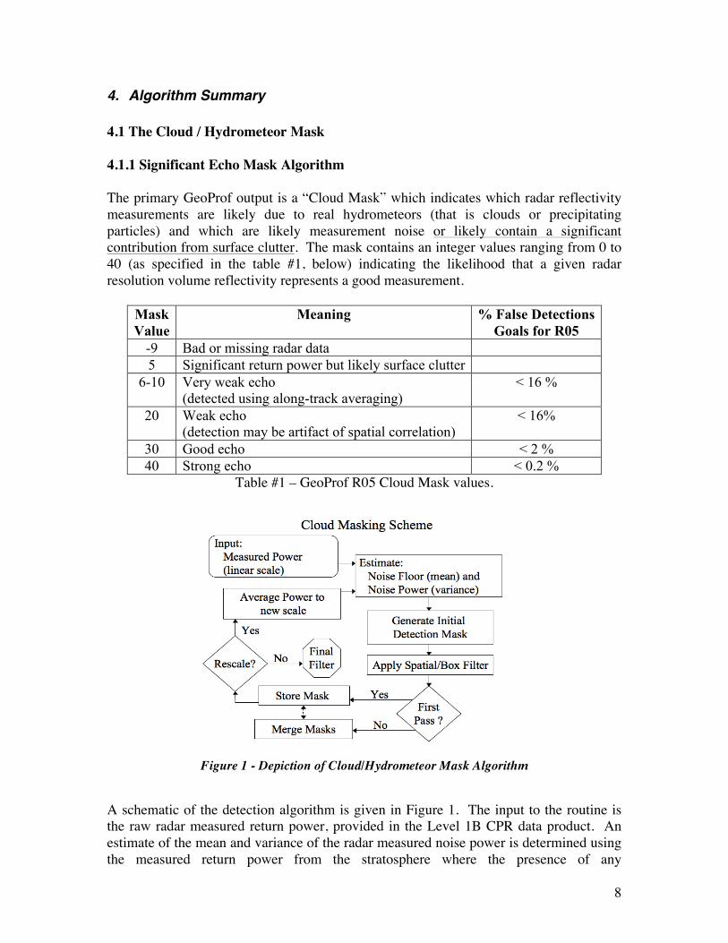
Figure 1 - Depiction of Cloud/Hydrometeor Mask Algorithm

A schematic of the detection algorithm is given in Figure 1. The input to the routine is the raw radar measured return power, provided in the Level 1B CPR data product. An estimate of the mean and variance of the radar measured noise power is determined using the measured return power from the stratosphere where the presence of any

9

hydrometeors—such as polar stratospheric clouds—would have a volume integrated backscatter cross-section much less than the detection threshold of the radar. Therefore, any power in these range bins is due primarily to microwave emission by the radar components, but also contains contributions from microwave emission by the Earth surface and gases such as water vapor in the atmospheric column. In R05, the mean noise power at each along-track sample is calculated using a mean filter that is ten range bins in the vertical for each profile. The standard deviation is calculated using the same vertical bins but all along-track bins (all good profiles) such that there is one value for each orbit. An initial set of hydrometeor detections is determined by comparing the target or return power with the noise power. Any range bin where the return power is greater than the noise power potentially contains backscattered power due to hydrometers. However, because of random fluctuations in the noise (which is Gaussian distributed), there is about a 16% chance that any range bin will have return power equal to one-standard deviation above the noise floor due solely to noise; i.e., a potential false detection. The detection algorithm starts by creating an initial cloud mask (with the same dimensions as the input return power matrix) with values ranging from zero to forty. Starting with R04, an estimate of surface clutter (contained in 1B-CPR product, see Tanelli et al. 2008) is subtracted from the return power in bins 2 through 5 above the surface. The original return power is kept in the surface bin, the bin 1 above the surface and all bins below the surface. For range bins where the return power is > than the mean noise power plus one standard deviation, the cloud mask is set to a value of 20; if the return power is > than two standard deviations the mask is set to 30; if > than three standard deviations the mask is set to 40; otherwise it is set to zero. We reserve values of 10 or less in the cloud mask to indicate clutter (value=5) OR the detection of clouds with signal power less then one standard deviation, which we discuss momentarily. To reduce the occurrence of false detections (which are uniformly randomly distributed) and to identify reliably range bins with true hydrometeors, a spatial box-filter is applied. Following Clothiaux et al. [1995, 2000], a box is centered over each range bin of a size Nw (range bins along track) by Nh (range bins in the vertical). We then count the number (No) of range bins in the box where the return power is > than the mean noise power plus one standard deviation, not counting the center range bin. The noise is expected to be Gaussian distributed and independent in each range bin, and so the probability (p) of any particular configuration with No, of the total (Nt = Nw Nh - 1) range bins would have a return power that is > than the mean noise power plus one standard deviation solely because of random noise is less than or equal to, (1) where G is the probability that the center pixel could be a false detection for a cloud mask value of level L (G(0) = 0.84, G(20) = 0.16, G(30)=0.028, G(40)=0.002). €

p ≤G L( ) 0.16N0( ) 0.84NT −N0( )

10

We expect that hydrometeor occurrence is highly spatially correlated over spatial scales of Nw by Nh range bins, and it is likely that, if a cloud is present, many range bins in the box will contain significant backscatter power. Thus, if p given by Eq. 1 is found to be less than some threshold value (i.e., p < pthresh), then the center range bin is unlikely to be noise and a hydrometeor (or other target) is likely present. In this situation, the cloud mask for the center range bin is then set to a value of 20 if it was zero in the initial cloud mask; otherwise the value in the initial cloud mask is retained. Likewise, if p >= pthresh, then the measured power could well be noise and the cloud mask is set to zero, regardless of the initial cloud mask value. Following Clothiaux et al. [1995, 2000] this box filter is applied to the data several times in succession. In each pass of the box filter some nominally false-detections are removed, and the effect of removing these detections is propagated to nearby pixels in the next pass. After a few passes one begins to remove more cloud (i.e. generate more failed detections) than to remove true false-detections. Like Clothiaux et al. we found 2 or 3 passes appeared nominal. The algorithm described is identical to that given by Clothiaux et al. [1995, 2000] except for the (center pixel) power weight in equation (1), that is, the factor G. Here the center pixel is given it full weight in order to reduce “corner removal” as discussed in detail in Marchand et al. [2008]. Having visually examined data from eight aircraft flights and months’ worth of ground-based radar data (both modified to look like less-sensitive CloudSat measurements, including the oversampling), as well as early mission CloudSat observations, we have found that, (2) with = 7, = 5, = 20 and three passes of the box filter produces good results, by which we mean that the algorithm is stable and produces few failed detections and a low rate of false detections. To improve the detection capability, the CloudSat algorithm is also designed to average the raw return power in the along-track direction. The purpose of this portion of the algorithm is to find condensate that is horizontally extensive (well beyond the size of the single radar profile) but below the single-profile sensitivity limit of the radar. We used four levels of along track averaging with 3, 5, 7 and 9 bin wide averaging windows. At each level, a separate cloud mask is created and merged in sequence, starting with the cloud mask created without any along track averaging. That is, we create a new cloud mask based on 3-bin along track averaging and then merge this 3-bin-cloud-mask with a cloud mask created without any along tracking averaging (what one might call a 0-bin-cloud-mask). We then create a cloud mask based on 5-bin along track averaging and merge this 5-bin-cloud-mask with the already combined 3-bin + 0-bin mask, etc.

pthresh =G 0.16Nthresh( ) 0.84NT−Nthresh( )

wN hN threshN

11

By applying a moving average to the data, the noise and target power become increasingly spatially correlated, thereby violating the independence assumption used in the spatial filter, Eq. 1. By trial and error, we found that using along-track averages of 3, 5, 7, and 9 bins for CloudSat required increasing Nthresh in order to compensate for the additional correlation. In R05 the required Nthresh is increased by 3+2.5*level (rounding up), where level goes from 1 to 4 and level 1 indicate a 3-bin along track average. This value is larger than that used in R04 (and earlier revisions) in order to reduce the false detection rate of the spatially-averaged detections to be close to that for level 20 detections. In addition to increasing Nthresh, we also only allow range bins to be marked as containing a likely hydrometeor in the moving averaged cloud masks if they initially contain a significant return. Thus, unlike the cloud mask created without along track averaging, no range bin in the n-bin-average mask can have a value greater than zero simply because it is surrounded by other likely detections. In order to merge each new moving-average mask with a previous mask, the new mask is compared with a reduced resolution version of the previous mask. This “reduced resolution previous mask” is constructed by taking a moving-average of the previous mask. The merged or combined mask is then given by the previous mask plus those range bins found to have both (a) values greater than zero in the new mask and (b) values of zero in the “reduced resolution version of the previous mask”. This last step prevents objects identified in the previous mask from being artificially expanded by the moving-average process. The new detections are given a cloud mask value of 11 minus the mask level number (which varies from 1 up to 4). Thus, cloud mask values of 6 to 10 indicate weak targets and specify the number of along-track bins averaged. Finally, after all levels are complete, the cloud mask is run through the spatial box filter a final time. This final filtering does allow pixels to be turned ON because of position (e.g., if a seemingly cloud-free pixel is completely surrounded by likely detections). 4.1.2 Surface Clutter Identification The nature of the CloudSat measurements near the surface is an important issue. The outgoing radar pulse is not a perfect square wave, but has a finite rise time. Because the surface is typically two to five orders of magnitude more reflective than hydrometeors, interaction between the surface and the edge of the radar pulse (which extends outside the nominal 480 m resolution volume) can contribute significant signal relative to that of potential near-surface hydrometeors. Measurements in the range bin closest to the surface and, because of oversampling, the bin directly above this bin, are expected to be dominated by the surface return. However, it is only for the fifth range bin (~ 1.2 km) above the surface that the signal returns approximately to the nominal sensitivity. Surface clutter is identified by a value of 5 in the CloudSat Hydrometeor Mask. The presence of a value of 5 means that there is significant return (scattered) power in the range bin, but it likely that this power has a significant component arise from scattering by the surface. That is, while Hydrometeors MAY also be present (it is often difficult to know) the measured reflectivity should NOT be take as that due to hydrometeors alone.

12

In R04, all detections below roughly the 99th percentile of the clear-sky return were set to a value of 5 – with separate threshold for ocean and land surfaces. Details (and threshold) values are given by Marchand [2008]. While this threshold is conservative in the sense that it should keep the false detection rate (by volume) below 1%, it also means that typically only rain and heavy drizzle can be detected in the third bin above the surface (~ 720 m) and moderate drizzle in the fourth bin (~ 860 m). Experience with R04 showed that this approach worked poorly over land surfaces, and in particular, over land surface where changes in elevation exceed 100 meters between neighboring radar profiles. In R05, the algorithm was changed in three ways. First, the thresholds over land where divided into to categories: “Smooth” land where the change in surface elevation (maximum – minimum) is 50 meters or less over 7 consecutive CloudSat profiles and “Rough” where the elevation change is larger. Second, the threshold was changed from 99% to 99.5%. Lastly, it was recognized the clutter always (or nearly always) increases toward the surface, whereas the scattering from hydrometeors are often observed to remain steady or decrease as one approaches the surface. The decrease is likely due the impact of attenuation. Thus, a third condition was added where the observed reflectivity (after subtraction of the Level 1B surface clutter estimate) had to increase (as one moves toward the surface) by at least 2 dB for the 99.5% clutter threshold to be applied. Finally, in R04 the surface height over land was based on the 1B CPR SurfaceBin variable, which is determined as the height bin (near the surface) with the largest reflectivity. However, in cases where the radar is heavily attenuated the strongest return may not be at the surface. Thus, the R04 algorithm required the 1B CPR SurfaceBin to agree within 2-bins of the Surface Digital Elevation Map (DEM). If it was not, the DEM height was used. Unfortunately, the DEM in R04 often had errors of more that 2 bins, causing many errors near the surface. In R05 the DEM has been greatly improved. Nonetheless there are still places with poor DEM values. The R05 GeoProf algorithm selects the surface height (over land) as whichever is lower the DEM or the 1B CPR SurfaceBin. 4.2 Variables related to the MODIS Cloud Mask CloudSat follows in orbit behind the EOS PM (Aqua) satellite. Aqua hosts the MODerate resolution Imaging Spectrometer (MODIS) and data acquired by MODIS are ingested into the operational CloudSat processing stream. The GeoProf product incorporates output form the MODIS cloud mask product (MOD35; Ackerman et al, 1998) as a quality/confidence check of the CloudSat GeoProf output. MODIS cloud mask data are available at 1 km (day and night) and 250m (daytime only) horizontal resolutions. The MODIS cloud mask includes 48-bit word (Table 1) for each 1km MODIS pixel. Table 1 provides a description of the information contained in the bitwise elements of the 48-bit word. Details of this product can be found in Ackerman et al. (1998). Given the nominal CloudSat footprint of 1.4 km across by 1.8 km along track [Tanelli et al. 2008], several MODIS 1 km pixels need to be examined to determine the likelihood that the CloudSat footprint is only partially filled with hydrometeors. It is expected that

13

some fraction of the hydrometeor-filled resolution volumes sampled by CloudSat will have a reflectivity below the minimum detectable signal of the CPR and will go undetected.

48 BIT CLOUD MASK FILE SPECIFICATION

BIT FIELD DESCRIPTION KEY RESULT 0 Cloud Mask Flag 0 = not determined

1 = determined 1-2 Unobstructed FOV Quality Flag 00 = cloudy

01 = uncertain clear 10 = probably clear 11 = confident clear

PROCESSING PATH FLAGS 3 Day / Night Flag 0 = Night / 1 = Day 4 Sun glint Flag 0 = Yes / 1 = No 5 Snow / Ice Background Flag 0 = Yes/ 1 = No

6-7 Land / Water Flag 00 = Water 01 = Coastal 10 = Desert 11 = Land

ADDITIONAL INFORMATION 8 Non-cloud obstruction Flag (heavy aerosol) 0 = Yes / 1 = No 9 Thin Cirrus Detected (near infrared) 0 = Yes / 1 = No

10 Shadow Found 0 = Yes / 1 = No 11 Thin Cirrus Detected (infrared) 0 = Yes / 1 = No 12 Spare (Cloud adjacency) (post launch)

1-km CLOUD FLAGS 13 Cloud Flag - simple IR Threshold Test 0 = Yes / 1 = No 14 High Cloud Flag - CO2 Threshold Test 0 = Yes / 1 = No 15 High Cloud Flag - 6.7 µm Test 0 = Yes / 1 = No 16 High Cloud Flag - 1.38 µm Test 0 = Yes / 1 = No 17 High Cloud Flag - 3.9-12 µm Test 0 = Yes / 1 = No 18 Cloud Flag - IR Temperature Difference 0 = Yes / 1 = No 19 Cloud Flag - 3.9-11 µm Test 0 = Yes / 1 = No 20 Cloud Flag - Visible Reflectance Test 0 = Yes / 1 = No 21 Cloud Flag - Visible Ratio Test 0 = Yes / 1 = No 22 Cloud Flag - Near IR Reflectance Test 0 = Yes / 1 = No 23 Cloud Flag - 3.7-3.9 µm Test 0 = Yes / 1 = No

ADDITIONAL TESTS 24 Cloud Flag - Temporal

Consistency 0 = Yes / 1 = No

25 Cloud Flag - Spatial Variability 0 = Yes / 1 = No 26-31 Spares

250-m CLOUD FLAG - VISIBLE TESTS

32 Element(1,1) 0 = Yes / 1 = No 33 Element(1,2) 0 = Yes / 1 = No 34 Element(1,3) 0 = Yes / 1 = No 35 Element(1,4) 0 = Yes / 1 = No 36 Element(2,1) 0 = Yes / 1 = No 37 Element(2,2) 0 = Yes / 1 = No 38 Element(2,3) 0 = Yes / 1 = No 39 Element(2,4) 0 = Yes / 1 = No 40 Element(3,1) 0 = Yes / 1 = No 41 Element(3,2) 0 = Yes / 1 = No 42 Element(3,3) 0 = Yes / 1 = No 43 Element(3,4) 0 = Yes / 1 = No 44 Element(4,1) 0 = Yes / 1 = No 45 Element(4,2) 0 = Yes / 1 = No 46 Element(4,3) 0 = Yes / 1 = No 47 Element(4,4) 0 = Yes / 1 = No

Table 1. Bitwise description of the elements of the MODIS cloud mask. (adapted from Ackerman et al., 1998)

14

Studies suggest that these clouds will be composed of primarily near-tropopause cirrus and liquid phase mid-level and boundary layer clouds. Stephens et al [2001] suggest that this characteristic of the CloudSat data does not detract from the main mission of the project – namely to characterize the radiative heating of the atmospheric column. The algorithm to compare the MODIS cloud mask and the CPR begins with a check of the status of the MODIS cloud mask and processing path used by the MODIS mask algorithm for the 15 1 km MODIS pixels nearest to the center of the CPR profile in question. A weighting is assigned to each pixel based on its location relative to the CloudSat footprint and the likelihood the pixel is within the CPR footprint. The schematic in Figure 2 illustrates the geometry of the problem accounting for the pointing uncertainty of the CPR of ~500 m. Once the pixel weighting is determined, bit 0 of each MODIS pixel is examined to ensure that the MODIS mask has been implemented and the processing path for that pixel is determined by examining bits 3-7 (see Table 1). The processing path bits identify which of the spectral tests are applicable. Bit 8 is also examined to ensure that heavy aerosol (smoke or dust) was not present to significantly contaminate the visible channel radiances. By examining the spectral tests for each of the relevant MODIS pixels it is possible to develop a broad characterization of the CloudSat scene. The level of detail that we can attain with this characterization depends largely on the processing path taken by the MODIS cloud mask algorithm (Table 2), with the processing path depending on the time of day and the surface ecosystem. Day

Ocean Night Ocean

Day Land

Night Land

Polar Day

(snow)

Polar Night

(snow)

Coast Day

Coast Night

Desert Day

Desert Night

BT11 (Bit 13) ü ü BT 13.9 (Bit 14) ü ü ü ü ü ü ü ü ü ü BT6.7 (Bit 15) ü ü ü ü ü ü ü ü ü ü R1.38 (Bit 16) ü ü ü ü ü BT3.7 - BT12 (Bit 17) ü ü ü BT8 - 11 & BT11 - 12 (Bit 18)

ü ü ü ü ü ü ü ü

Figure 2. Schematic of the CloudSat-MODIS pixel configuration. The circles represent the MODIS pixels. The green rectangular area represents the 1.1 km region that is most heavily weighted for the associated CloudSat CPR profile. The darker blue region are less heavily weighted. The light green area represents an outer region which may contribute due to pointing uncertainty.

15

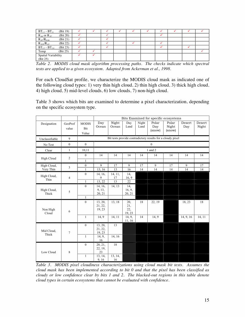
BT3.7 - BT11 (Bit 19) ü ü ü ü ü ü ü ü ü ü R.66 or R.87 (Bit 20) ü ü ü R.87/R0.66 (Bit 21) ü ü R.935/R.87 (Bit 22) ü ü ü ü BT3.7 - BT3.9 (Bit 23) ü ü ü ü Temp (Bit 25) ü ü ü Spatial Variability (Bit 25)

ü ü

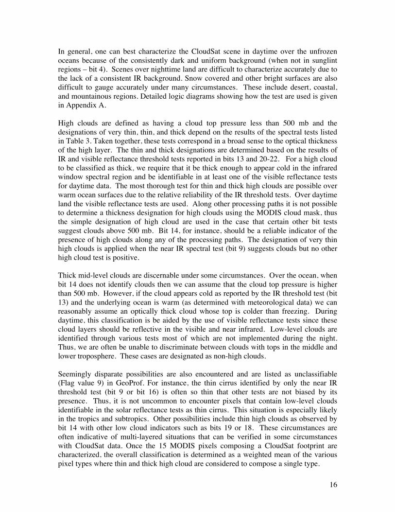
Table 2. MODIS cloud mask algorithm processing paths. The checks indicate which spectral tests are applied to a given ecosystem. Adapted from Ackerman et al., 1998. For each CloudSat profile, we characterize the MODIS cloud mask as indicated one of the following cloud types: 1) very thin high cloud, 2) thin high cloud, 3) thick high cloud, 4) high cloud, 5) mid-level clouds, 6) low clouds, 7) non-high cloud. Table 3 shows which bits are examined to determine a pixel characterization, depending on the specific ecosystem type.

Bits Examined for specific ecosystems

Designation GeoProf value

MODIS Bit

Value

Day Ocean

Night Ocean

Day Land

Night Land

Polar Day

(snow)

Polar Night (snow)

Desert Day

Desert Night

Unclassifiable 9 Bit tests provide contradictory results for a cloudy pixel

No Test 0 0 0

Clear 1 10,11 1 and 2

High Cloud 2 0 14 14 14 14 14 14 14 14

1 High Cloud, Very Thin 3 0 9 17 9 17 9 17 9 17

1 13, 16 13 16 14 14 14 14 14

High Cloud, Thin 4

0 14, 16, 9

14, 11, 17

14, 16, 9

1 13, 22 13 22

High Cloud, Thick 5

0 14, 16, 9, 13, 20, 21

14, 13 14, 16, 9, 20, 21

1

Non High Cloud 6

0 13, 20, 21, 22, 19, 23

13, 18 20, 21, 22,

19, 23

18 22, 19 18, 23 18

1 14, 9 14, 11 14, 9, 11, 16

14 14, 9 14, 9, 16 14, 11

Mid Cloud, Thick 7

0 13, 20, 21, 22, 19, 23

13

1 14, 9, 16

14, 16

Low Cloud 8

0 20, 21, 22, 19,

23

18

1 13, 14, 9, 16

13, 14, 16

Table 3. MODIS pixel cloudiness characterizations using cloud mask bit tests. Assumes the cloud mask has been implemented according to bit 0 and that the pixel has been classified as cloudy or low confidence clear by bits 1 and 2. The blacked-out regions in this table denote cloud types in certain ecosystems that cannot be evaluated with confidence.

16

In general, one can best characterize the CloudSat scene in daytime over the unfrozen oceans because of the consistently dark and uniform background (when not in sunglint regions – bit 4). Scenes over nighttime land are difficult to characterize accurately due to the lack of a consistent IR background. Snow covered and other bright surfaces are also difficult to gauge accurately under many circumstances. These include desert, coastal, and mountainous regions. Detailed logic diagrams showing how the test are used is given in Appendix A. High clouds are defined as having a cloud top pressure less than 500 mb and the designations of very thin, thin, and thick depend on the results of the spectral tests listed in Table 3. Taken together, these tests correspond in a broad sense to the optical thickness of the high layer. The thin and thick designations are determined based on the results of IR and visible reflectance threshold tests reported in bits 13 and 20-22. For a high cloud to be classified as thick, we require that it be thick enough to appear cold in the infrared window spectral region and be identifiable in at least one of the visible reflectance tests for daytime data. The most thorough test for thin and thick high clouds are possible over warm ocean surfaces due to the relative reliability of the IR threshold tests. Over daytime land the visible reflectance tests are used. Along other processing paths it is not possible to determine a thickness designation for high clouds using the MODIS cloud mask, thus the simple designation of high cloud are used in the case that certain other bit tests suggest clouds above 500 mb. Bit 14, for instance, should be a reliable indicator of the presence of high clouds along any of the processing paths. The designation of very thin high clouds is applied when the near IR spectral test (bit 9) suggests clouds but no other high cloud test is positive. Thick mid-level clouds are discernable under some circumstances. Over the ocean, when bit 14 does not identify clouds then we can assume that the cloud top pressure is higher than 500 mb. However, if the cloud appears cold as reported by the IR threshold test (bit 13) and the underlying ocean is warm (as determined with meteorological data) we can reasonably assume an optically thick cloud whose top is colder than freezing. During daytime, this classification is be aided by the use of visible reflectance tests since these cloud layers should be reflective in the visible and near infrared. Low-level clouds are identified through various tests most of which are not implemented during the night. Thus, we are often be unable to discriminate between clouds with tops in the middle and lower troposphere. These cases are designated as non-high clouds. Seemingly disparate possibilities are also encountered and are listed as unclassifiable (Flag value 9) in GeoProf. For instance, the thin cirrus identified by only the near IR threshold test (bit 9 or bit 16) is often so thin that other tests are not biased by its presence. Thus, it is not uncommon to encounter pixels that contain low-level clouds identifiable in the solar reflectance tests as thin cirrus. This situation is especially likely in the tropics and subtropics. Other possibilities include thin high clouds as observed by bit 14 with other low cloud indicators such as bits 19 or 18. These circumstances are often indicative of multi-layered situations that can be verified in some circumstances with CloudSat data. Once the 15 MODIS pixels composing a CloudSat footprint are characterized, the overall classification is determined as a weighted mean of the various pixel types where thin and thick high cloud are considered to compose a single type.

17

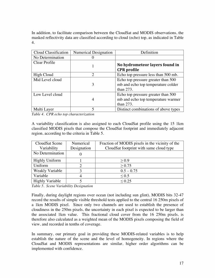
In addition, to facilitate comparison between the CloudSat and MODIS observations, the masked reflectivity data are classified according to cloud (echo) top, as indicated in Table 4.

Cloud Classification Numerical Designation Definition No Determination 0 Clear Profile

1 NohydrometeorlayersfoundinCPRprofile

High Cloud 2 Echo top pressure less than 500 mb. Mid Level cloud

3 Echo top pressure greater than 500 mb and echo top temperature colder than 273.

Low Level cloud 4

Echo top pressure greater than 500 mb and echo top temperature warmer than 273.

Multi Layer 5 Distinct combinations of above types Table 4. CPR echo top characterization A variability classification is also assigned to each CloudSat profile using the 15 1km classified MODIS pixels that compose the CloudSat footprint and immediately adjacent region, according to the criteria in Table 5.

CloudSat Scene Variability

Numerical Designation

Fraction of MODIS pixels in the vicinity of the CloudSat footprint with same cloud type

No Determination 0 Highly Uniform 1 ≥ 0.9 Uniform 2 ≥ 0.75 Weakly Variable 3 0.5 – 0.75 Variable 4 ≤ 0.5 Highly Variable 5 ≤ 0.25

Table 5. Scene Variability Designation Finally, during daylight regions over ocean (not including sun glint), MODIS bits 32-47 record the results of simple visible threshold tests applied to the central 16 250m pixels of a 1km MODIS pixel. Since only two channels are used to establish the presence of cloudiness in the 250m pixels, the uncertainty in each pixel is expected to be larger than the associated 1km value. This fractional cloud cover from the 16 250m pixels, is therefore also calculated as a weighted mean of the MODIS pixels composing the field of view, and recorded in tenths of coverage. In summary, our primary goal in providing these MODIS-related variables is to help establish the nature of the scene and the level of homogeneity. In regions where the CloudSat and MODIS representations are similar, higher order algorithms can be implemented with confidence.

18

5. Data Product Output Format 5.1 Format Overview The CPR Level 2 GEOPROF Product contains an estimate of the radar reflectivity factor and cloud mask. The format chosen for CPR Level 2 GEOPROF data is similar to that for CPR Level 1 B data. The format consists of metadata, which describes the data characteristics, and swath data, which includes the radar reflectivity factor, cloud mask and other information. The following schematic illustrates how GEOPROF data is formatted using HDF EOS. The variable nray is the number of radar profiles (frames, rays) in a granule. Each block is a 0.16 s average of radar data. Table 6. CPR Level 2 GEOPROF HDF-EOS Data Structure

Data Granule

Swath Data

Time Table: nray 10 bytes

Geolocation 2 × nray 4-byte float

SEM

Radar Reflectivity 125 × nray 2-byte integer

Quality assurance QA 125 × nray 1 byte integer

CPR Cloud Mask 125 × nray 1 byte integer

SEM-MODIS

MODIS scene characterizations (Table 3) 1 byte

nray CPR echo top characterizations (Table 4) 1 byte MODIS scene variability (Table 5) 1 byte MODIS 250m cloud fraction 1 byte

5.2 CPR Level 2 GEOPROF HDF-EOS Data Contents q Time (Vdata data, array size nray, record size 10 byte): Time is determined based on VTCW time. See Table 2 of Li and Durden (2001) for data format. q Geolocation (SDS, array size 2 × nray, 4-byte float): As documented in Li and Durden (2001), geolocation is defined as the Earth location of the center of the IFOV at the altitude of the Earth ellipsoid. The first dimension is latitude and longitude, in that order. The next dimension is ray number. Values are represented as floating point decimal degrees. Off earth is represented as less than or equal to -9999.9.

19

Latitude is positive north, negative south. Longitude is positive east, negative west. A point on the 180th meridian is assigned to the western hemisphere. q SEM product

§ Radar Reflectivity (SDS, array size 125 × nray, 2-byte integer) Radar reflectivity factor Ze is calculated with the echo power (Pr) and other input data as described in Level 1B CPR Process Description and Interface Control Document (Li and Durden, 2001).

§ Quality assurance QA (SDS, array size 125 × nray, 1-byte integer) Quality assurance QA is the likelihood that a CloudSat resolution volume with a particular value of peff contains hydrometeors as compared to MMCR data.

§ CPR Cloud Mask (SDS, array size 125 × nray, 1-byte integer) Each CPR resolution volume is assigned 1-bit mask value: 0 = No cloud detected 1 = Cloud detected q SEM-MODIS product

§ MODIS scene characterizations (SDS, 1-byte integer) This data includes MODIS pixel cloudiness characterizations using cloudmask bit tests. See Table 3 for a detailed specification.

§ CPR echo top characterizations (SDS, 1-byte integer) See Table 4 for the detail specification.

§ MODIS scene variability (SDS, 1-byte integer) MODIS scene variability includes the variability classification assigned to the CloudSat scene using the 1 km classified MODIS pixels that compose the CloudSat footprint and immediately adjacent region. See Table 5 for detail specification.

§ MODIS 250m cloud fraction (SDS, 1-byte integer) MODIS 250 m cloud fraction includes cloud fraction calculated with MODIS 250m pixels.

20

6. Summary of changes from previous versions Summary of changes from R03 to R04

An estimate of surface clutter (contained in 1B-CPR R04) is now subtracted from the return power in bins 2 through 5 above the surface. The original return power is kept in the surface bin, the bin 1 above the surface and all bins below the surface. See text below for more discussion. There are four additional variables in the R04: Clutter_reduction_flag

This flag has a value of 1, whenever an estimate of surface clutter has been subtracted from the measured return power (in bins 2 through 5 above the surface). It is zero, otherwise.

SurfaceHeightBin_fraction

This variable indicates the fractional location of the surface with in the pixel given by the variable “SurfaceHeightBin”. This value is estimated in the clutter estimation processes. The altitude of the surface with respect to mean sea level is thus given by Height(SurfaceHeightBin) + RangeBinSize*SurfaceHeightBin_fraction. This variable is real valued. Values less than -5 should not be used and indicate that the 2B GEOPROF code did consider the fraction to be valid.

MODIS_cloud_flag

This variable contains the MODIS summary cloud flag (bits 3 and 4 from MOD35) for the CloudSat column. Values are:

0 = Clear High Confidence 1 = Clear Low Confidence 2 = Cloudy Low Confidence 3 = Cloudy High Confidence

Note: the variable “MODIS_cloud_fraction” in 2B GEOPROF R03 and R04 is the fraction of VISIBLE pixels in the MODIS 250 m mask that are cloudy. This cloud fraction is only valid during the day and does not include cloud detection from at IR channels.

Sigma-Zero

21

This variable is a pass through from 1B-CPR. It is the estimated surface reflectance (in units of dBZ * 100).

Summary of changes from R04 to R05

R05 has a significantly improved false detection rate, primarily for weak detections, especially those identified using the along track averaging. This is due primarily to improved estimates of the radar noise floor power variance (using all profiles rather than moving average) and re-optimized filter parameters (see section 4.1.1). R05 also feature a new and improved surface clutter identification approach (see section 4.1.2). R05 also now includes an along track (profile-by-profile) estimate of the radar Minimum Detectable Signal (MDS). Other improves follow from changes to 1B CPR and ancillary data including and improved Digital Elevation Map and various changes to the data quality flags.

22

7. References Ackerman, S. A., K. I. Strabala, W. P. Menzel, R. A. Frey, C. C. Moeller, L. E. Gumley,

1998: Discriminating clear sky from clouds with MODIS. J. Geophys. Res., 103, 32141-32157.

Clothiaux, E. E., M. A. Miller, B. A. Albrecht, T. P. Ackerman, J. Verlinde, D. M. Babb,

R. M. Peters, and W. J. Syrett, 1995: An evaluation of a 94-GHz radar for remote sensing of cloud properties. J. Atmos. Oceanic. Technol., 12, 201-229.

Clothiaux EE, Ackerman TP, Mace GG, Moran KP, Marchand RT, Miller MA, Martner

BE, 2000 “Objective determination of cloud heights and radar reflectivities using a combination of active remote sensors at the ARM CART sites,” J APPL METEOROL 39 (5): 645-665 MAY 2000

Li, L. and S. Durden, 2001: Level 1 B CPR Process Description and Interface Control

Document. Jet Propulsion Laboratory. Marchand, R., G.G. Mace, T. Ackerman, and G. Stephens (2008), Hydrometeor

Detection Using Cloudsat—An Earth-Orbiting 94-GHz Cloud Radar. J. Atmos. Oceanic Technol., 25, 519–533.

Marchand, R., S. Tanelli, G. Mace, and G. Stephens (2018?), An Updates to the

Operational CloudSat Hydrometeor Detection Algorithm, GeoProf. Manuscript in preparation.

Tanelli, S., Durden, S. L., Im, E., Pak, K. S., Reinke, D. G., Partain, P., Haynes, J. M.,

and Marchand, R. T. (2008), CloudSat's Cloud Profiling Radar After Two Years in Orbit: Performance, Calibration, and Processing, IEEE Trans. on Geoscience and Remote Sensing, 46(11), p. 3560 - 3573, doi:10.1109/TGRS.2008.2002030.

23

8. Acronym List SEM – Significant Echo Mask MODIS – Moderate-Resolution Imaging Spectroradiometer

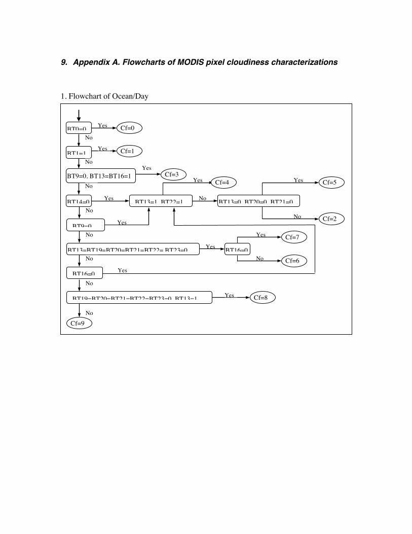
9. Appendix A. Flowcharts of MODIS pixel cloudiness characterizations

1. Flowchart of Ocean/Day

BT19=BT20=BT21=BT22=BT23=0, BT13=1 Cf=8

Cf=9

No

No

Yes

BT9=0, BT13=BT16=1 Yes

Cf=3

No

BT1=1

No

Cf=1 Yes

No

BT0=0 Yes Cf=0

BT14=0 Yes

No

Yes

BT13=1, BT22=1 BT13=0, BT20=0, BT21=0

Cf=5

Cf=2

No

Cf=4 Yes

Yes BT16=0

BT13=BT19=BT20=BT21=BT22= BT23=0 No

Yes

Yes

Cf=6

Cf=7

BT16=0

No

No

BT9=0 Yes

No

25

2. Flowchart of Ocean/Night

No

No

Yes BT11=0, BT17=0

BT13=0, BT16=1

BT14=0

BT17=0, BT13=1

BT13=0

BT13=0, BT18=0, BT11=1

BT18=0, bt13=1, BT16=1

Cf=5

Cf=3

Cf=4

Cf=2

Cf=7

Cf=9

Cf=8

BT0=0

Yes BT1=1

Cf=0 Yes

Cf=1

No

No

No

Yes

Cf=6

No

No

No

Yes

Yes

Yes

No

Yes

Yes

26

3. Flowchart of Land/Day

BT0=0

BT1=1

Cf=0 Yes

Yes Cf=1

No

No

Yes

Yes

Cf=3

Cf=2

No

No

No

BT14 + BT15 +BT16 <= 2

Cf=4

Cf=5

Cf=6

Cf=9

No

Yes

BT9 = 0 BT16 + BT19 + BT20 + BT21 + BT 22 = 5 Yes

No

BT20 + BT21 = 2 Yes

BT14 + BT15 +BT16 <= 1 And BT20 + BT21 <=1

Yes

BT19 + BT20 + BT21 + BT 22 <= 2 And BT9 + BT14 + BT16 == 3

4. Flowchart of Land/Night

Yes

Yes

No

No

BT0=0

BT1=1

Cf=0 Yes

Yes Cf=1

No

No

Yes Cf=2

No

BT14=0

Cf=9

Cf=6

Cf=3 BT17=0

BT18=0

27

BT0=0

BT1=1

Cf=0 Yes

Yes Cf=1

No

No Yes

Yes

Yes

No

Cf=2

No

No

BT14=0

Cf=9

Cf=6

Cf=3 BT9=0

BT19=0 and BT22=0

BT0=0

BT1=1

Cf=0 Yes

Yes Cf=1

No

No

Yes Cf=2

No

BT14=0

Yes

No

Cf=9

Cf=3 BT17=0

BT0=0

BT1=1

Cf=0 Yes

Yes Cf=1

No

No

Yes Cf=2

No

BT14=0

Yes

Yes

No

No

Cf=9

Cf=6

Cf=3 BT9=0

BT18=BT23=0 and BT16=1

BT0=0

BT1=1

Cf=0 Yes

Yes Cf=1

No

No

Yes Cf=2

No

BT14=0

Yes

Yes

No

No

Cf=9

Cf=6

Cf=3 BT17=0

BT18=0 and BT11=1

5. Flowchart of Polar/Day 6. Flowchart of Polar/Night

7. Flowchart of Desert/Day 8. Flowchart of Desert/Night