LESSON 5 Multiple Regression Copyright © 2006 Pearson Addison-Wesley. All rights reserved. 7-1.

LESSON 5

•Multiple Regression

Copyright © 2006 Pearson Addison-Wesley. All rights reserved. 7-1


Multiple Regression

• We know how to regress Y on a constant and a single X variable

• 1 is the change in Y from a 1-unit change in X

Y 0 1·X


Multiple Regression (cont.)

• Usually we will want to include more than one independent variable.

• How can we extend our procedures to permit multiple X variables?


Gauss–Markov DGP with Multiple X ’s

Y 0

1X

1i

2X

2i

kX

ki

i

E(i) 0

Var(i) 2

Cov(i,

j) 0, for i j

X1X

k fixed across samples (so we can

treat them like constants).


BLUE Estimators

• Ordinary Least Squares is still BLUE

• The OLS formula for multiple X ’s requires matrix algebra, but is very similar to the formula for a single X


BLUE Estimators (cont.)

• Intuitions from the single variable formulas tend to generalize to multiple variables.

• We’ll trust the computer to get the formulas right.

• Let’s focus on interpretation.


Single Variable Regression


Multiple Regression

• 1 is the change in Y from a 1-unit change in X1

Y 0 1X1



• How can we interpret 1 now?

• 1 is the change in Y from a 1-unit change in X1 , holding X2…Xk FIXED

Y 0 1X1 2 X2 k Xk



• How do we implement multiple regression with our software?


Example: Growth

• Regress GDP growth from 1960–1985 on– GDP per capita in 1960 (GDP60)

– Primary school enrollment in 1960 (PRIM60)

– Secondary school enrollment in 1960 (SEC60)

– Government spending as a share of GDP (G/Y)

– Number of coups per year (REV)

– Number of assassinations per year (ASSASSIN)

– Measure of Investment Price Distortions (PPI60DEV)


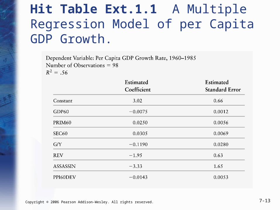
Hit Table Ext.1.1 A Multiple Regression Model of per Capita GDP Growth.


Example: Growth (cont.)

• A 1-unit increase in GDP in 1960 predicts a 0.008 unit decrease in GDP growth, holding fixed the level of PRIM60, SEC60, G/Y, REV, ASSASSIN, and PPI60DEV.

3.02 – 0.008· 60

0.025· 60 0.031· 60

- 0.119· / –1.950·

- 3.330· – 0.014· 60

GDP Growth GDP

PRIM SEC

G Y REV

ASSASSIN PPI DEV



• Before we controlled for other variables, we found a POSITIVE relationship between growth and GDP per capita in 1960.

• After controlling for measures of human capital and political stability, the relationship is negative, in accordance with “catch up” theory.



• Countries with high values of GDP per capita in 1960 ALSO had high values of schooling and a low number of coups/assassinations.

• Part of the relationship between growth and GDP per capita is actually reflecting the influence of schooling and political stability.

• Holding those other variables constant lets us isolate the effect of just GDP per capita.


Example: Growth

• The Growth of GDP from 1960–1985 was higher:

1. The lower starting GDP, and

2. The higher the initial level of human capital.

• Poor countries tended to “catch up” to richer countries as long as the poor country began with a comparable level of human capital, but not otherwise.



• Bigger government consumption is correlated with lower growth; bigger government investment is only weakly correlated with growth.

• Politically unstable countries tended to have weaker growth.

• Price distortions are negatively related to growth.



• The analysis leaves largely unexplained the very slow growth of Sub-Saharan African countries and Latin American countries.

20

Omitted Variable Bias

The error ε arises because of factors that influence Y but are not

included in the regression function; so, there are always omitted

variables.

Sometimes, the omission of those variables can lead to bias in

the OLS estimator.

21

Omitted variable bias, ctd.

The bias in the OLS estimator that occurs as a result of an

omitted factor is called omitted variable bias. For omitted

variable bias to occur, the omitted factor “Z” must be:

1. A determinant of Y (i.e. Z is part of ε); and

2. Correlated with the regressor X (i.e. corr(Z,X) 0)

Both conditions must hold for the omission of Z to result in

omitted variable bias.

22

Omitted variable bias, ctd.

In the test score example:

1. English language ability (whether the student has English as

a second language) plausibly affects standardized test

scores: Z is a determinant of Y.

2. Immigrant communities tend to be less affluent and thus

have smaller school budgets – and higher STR: Z is

correlated with X.

Accordingly, 1 is biased. What is the direction of this bias?

What does common sense suggest?

If common sense fails you, there is a formula…

23

The omitted variable bias formula:

1 p

1 + uXu

X

If an omitted factor Z is both:

(1) a determinant of Y (that is, it is contained in u); and

(2) correlated with X,

then Xu 0 and the OLS estimator 1 is biased (and is not

consistent). The math makes precise the idea that districts with few ESL students (1) do better on standardized tests and (2) have smaller classes (bigger budgets), so ignoring the ESL factor results in overstating the class size effect.

Is this is actually going on in the CA data?

24

Measures of Fit for Multiple Regression

Actual = predicted + residual: Yi = iY + ie

Se = std. deviation of ie (with d.f. correction)

RMSE = std. deviation of ie (without d.f. correction)

R2 = fraction of variance of Y explained by X

2R = “adjusted R2” = R2 with a degrees-of-freedom correction

that adjusts for estimation uncertainty; 2R < R2

25

Se and RMSE

As in regression with a single regressor, the Se and the RMSE are

measures of the spread of the Y’s around the regression line:

2

2

1

2

1

i

ie

en

RMSE

en

S

26

R2 and 2R

The R2 is the fraction of the variance explained – same definition

as in regression with a single regressor:

R2 = explained SS/Total SS= = TSS

residualSS1 ,

The R2 always increases when you add another regressor

(why?) – a bit of a problem for a measure of “fit”

27

R2 and , ctd.

The 2R (the “adjusted R2”) corrects this problem by “penalizing”

you for including another regressor – the 2R does not necessarily

increase when you add another regressor.

Adjusted R2: ]

1

1)1[(1 22

kn

nRR

Note that 2R < R2, however if n is large the two will be very

close.

2R

28

Measures of fit, ctd.

Test score example:

(1) ·TestScore = 698.9 – 2.28STR,

R2 = .05, Se = 18.6

(2) ·TestScore = 686.0 – 1.10STR – 0.65PctEL,

R2 = .426, 2R = .424, Se = 14.5

What – precisely – does this tell you about the fit of regression (2) compared with regression (1)?

Why are the R2 and the 2R so close in (2)?

29

The Least Squares Assumptions for Multiple Regression

Yi = 0 + 1X1i + 2X2i + … + kXki + ui, i = 1,…,n

1. The conditional distribution of u given the X’s has mean

zero, that is, E(u|X1 = x1,…, Xk = xk) = 0.

2. (X1i,…,Xki,Yi), i =1,…,n, are i.i.d.

3. Large outliers are rare: X1,…, Xk, and Y have four moments:

E( 41iX ) < ,…, E( 4

kiX ) < , E( 4iY ) < .

4. There is no perfect multicollinearity.

Testing Hypotheses


t- test – individual testF-test – joint test

Dummy Variables

• Used to capture qualitative explanatory variables

• Used to capture any event that has only two possible outcomes

e.g. race, gender , geographic region of residence etc.

Use of Intercept Dummy

• Most common use of dummy variables.

• Modifies the regression model intercept parameter

e.g. Let test the “location”, “location” “location” model of real estate

Suppose we take into account location near say a university or golf course

• Pt = βo + β1 St +β2 Dt + εt

• St = square footage

• D = dummy variable to represent if the characteristic is present or not

• D = 1 if property is in a desirable neighborhood

• 0 if not in a desirable neighborhood

• Effect of the dummy variable is best seen by examining the E(Pt).

• If model is specified correctly, E(εt )

• = 0

• E(Pt ) = ( βo + β2 ) + β1 St when D=1

βo + β1 St when D = 0

• B2 is the location premium in this case.

• It is the difference between the Price of a house in a desirable are and one in a not so desirable area, all things held constant

• The dummy variable is to capture the shift in the intercept as a result of some qualitative variable

• Dt is an intercept dummy variable

• Dt is treated as any explanatory variable.

• You can construct a confidence interval for B2

• You can test if B2 is significantly different from zero.

• In such a test, if you accept Ho, then there is no difference between the two categories.

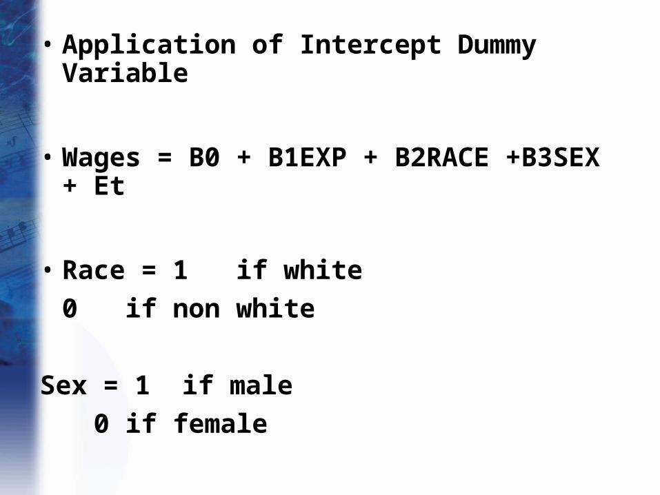
• Application of Intercept Dummy Variable

• Wages = B0 + B1EXP + B2RACE +B3SEX + Et

• Race = 1 if white

0 if non white

Sex = 1 if male

0 if female

• WAGES = 40,000 + 1487EXP + 1102RACE +1082SEX

• Mean salary for black female

40,000 + 1487 EXP

Mean salary for white female

41,102 + 1487EXP +1102

• Mean salary for Asian male

• Mean salary for white male

• What sucks more, being female or non white?

• Determining the # of dummies to use

• If h categories, then use h-1 dummies

• Category left out defines reference group

• If you use h dummies you’d fall into the dummy trap

Slope Dummy Variables

• Allows for different slope in the relationship

• Use an interaction variable between the actual variable and a dummy variable

e.g.

Pt = Bo + B1Sqfootage+B2(Sqfootage*D)+et

D= 1 desirable area, 0 otherwise

• Captures the effect of location and size on the price of a house

• E(Pt) = B0 + (B1+B2)Sqfoot if D=1

= BO + B1Sqfoot if D = 0

in the desirable area, price per square foot is b1+b2, and it is b1 in other areas

If we believe that a house location affects both the intercept and the slope then the model is

Pt = B0 +B1sqfoot +B2(sqfoot*D) + B3D +et

44

Dummies for Multiple Categories

• We can use dummy variables to control for something with multiple categories

• Suppose everyone in your data is either a HS dropout, HS grad only, or college grad

• To compare HS and college grads to HS dropouts, include 2 dummy variables

• hsgrad = 1 if HS grad only, 0 otherwise; and colgrad = 1 if college grad, 0 otherwise

45

Multiple Categories (cont)

• Any categorical variable can be turned into a set of dummy variables

• Because the base group is represented by the intercept, if there are n categories there should be n – 1 dummy variables

• If there are a lot of categories, it may make sense to group some together

• Example: top 10 ranking, 11 – 25, etc.

46

Interactions Among Dummies

• Interacting dummy variables is like subdividing the group

• Example: have dummies for male, as well as hsgrad and colgrad

• Add male*hsgrad and male*colgrad, for a total of 5 dummy variables –> 6 categories

• Base group is female HS dropouts

• hsgrad is for female HS grads, colgrad is for female college grads

• The interactions reflect male HS grads and male college grads

47

More on Dummy Interactions

• Formally, the model is y = 0 + 1male + 2hsgrad + 3colgrad + 4male*hsgrad + 5male*colgrad + 1x + u, then, for example:

• If male = 0 and hsgrad = 0 and colgrad = 0

• y = 0 + 1x + u


• y = 0 + 2hsgrad + 1x + u


• y = 0 + 1male + 3colgrad + 5male*colgrad + 1x + u

48

Other Interactions with Dummies

• Can also consider interacting a dummy variable, d, with a continuous variable, x

• y = 0 + 1d + 1x + 2d*x + u

• If d = 0, then y = 0 + 1x + u

• If d = 1, then y = (0 + 1) + (1+ 2) x + u

• This is interpreted as a change in the slope

49

y

x

y = 0 + 1x

y = (0 + 0) + (1 + 1) x

Example of 0 > 0 and 1 < 0

d = 1

d = 0

LESSON 5 Multiple Regression Copyright © 2006 Pearson Addison-Wesley. All rights reserved. 7-1.

Documents

Transcript of LESSON 5 Multiple Regression Copyright © 2006 Pearson Addison-Wesley. All rights reserved. 7-1.