Lesson 4 –Exponential Functions I · ... then an exponential function models the data best. ......

Lesson 4 –Exponential Functions I

149

Lesson 4 –Exponential Functions I Exponential functions play a major role in our lives. Population growth and disease processes are real-world problems that involve exponential change and can be modeled by exponential functions. Problems involving money, such as the growth of our savings account or the amount of interest we pay on a loan, can also be modeled by exponential functions. In this lesson, we begin our investigation of exponential functions by comparing them to linear functions, examining how they are constructed and how they behave. We then learn methods for evaluating exponential functions and solving equations that involve exponential functions. Lesson Topics:

Section 4.1: Linear Functions vs. Exponential Functions § Characteristics of Linear Functions § Comparing Linear and Exponential Growth § Using the Common Ratio to Identify Exponential Data § Horizontal Intercepts

Section 4.2: Characteristics of Exponential Functions Section 4.3: Solving Exponential Equations by Graphing

§ Graphing Using the TI83/84 Calculator § Viewing Window

Section 4.4: Applications of Exponential Functions

Lesson 4 –Exponential Functions I

150

Lesson 4 –Exponential Functions I - MiniLesson

151

Lesson 4 - Mini-Lesson

Section 4.1 – Linear Functions vs. Exponential Functions

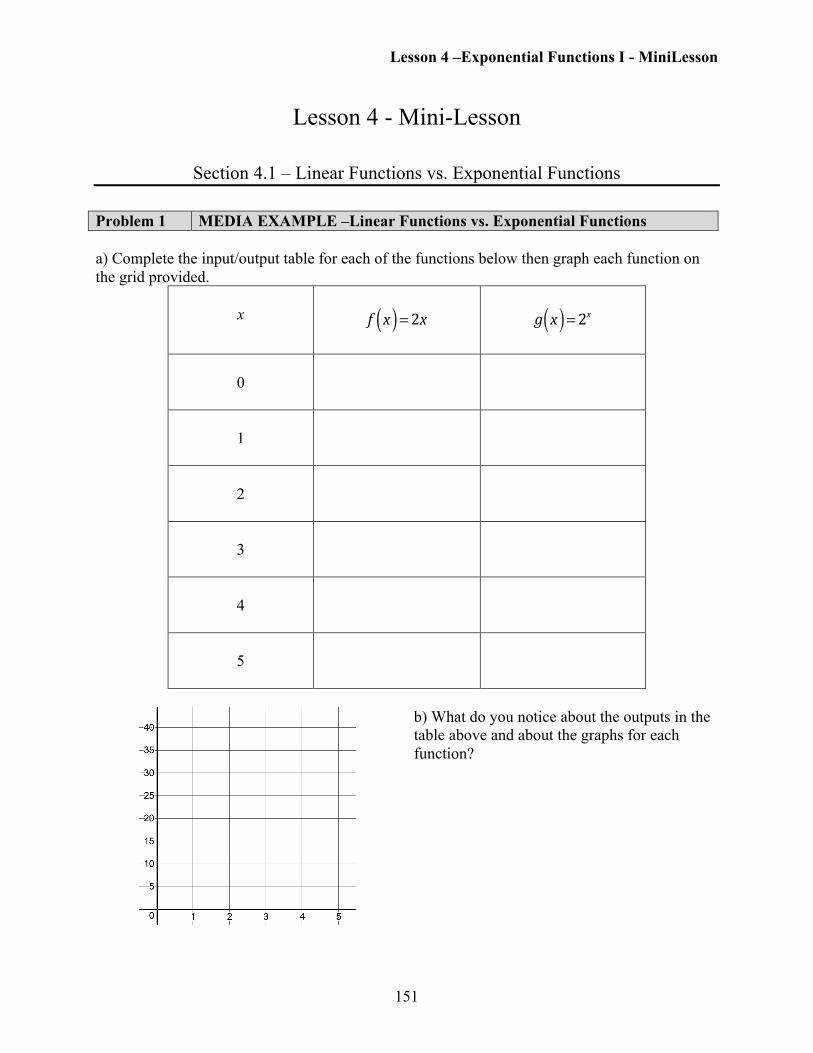
Problem 1 MEDIA EXAMPLE –Linear Functions vs. Exponential Functions a) Complete the input/output table for each of the functions below then graph each function on the grid provided.

x

!!f x( ) =2x

!!g x( ) =2x

0

1

2

3

4

5

b) What do you notice about the outputs in the table above and about the graphs for each function?


152

Exponential Functions vs. Linear Functions

The outputs for linear functions change via addition. The outputs for exponential functions change via multiplication.

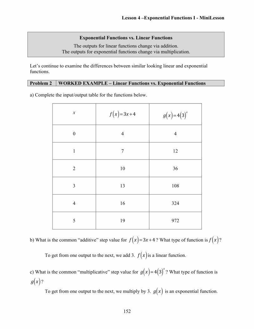
Let’s continue to examine the differences between similar looking linear and exponential functions. Problem 2 WORKED EXAMPLE – Linear Functions vs. Exponential Functions a) Complete the input/output table for the functions below.

x

!!f x( ) =3x +4

!!g x( ) = 4 3( )x

0

4

4

1

7

12

2

10

36

3

13

108

4

16

324

5

19

972

b) What is the common “additive” step value for !!f x( ) =3x +4 ? What type of function is!

f x( )?

To get from one output to the next, we add 3. !f x( ) is a linear function.

c) What is the common “multiplicative” step value for !!g x( ) = 4 3( )x ? What type of function is

!g x( ) ?

To get from one output to the next, we multiply by 3. !g x( ) is an exponential function.


153

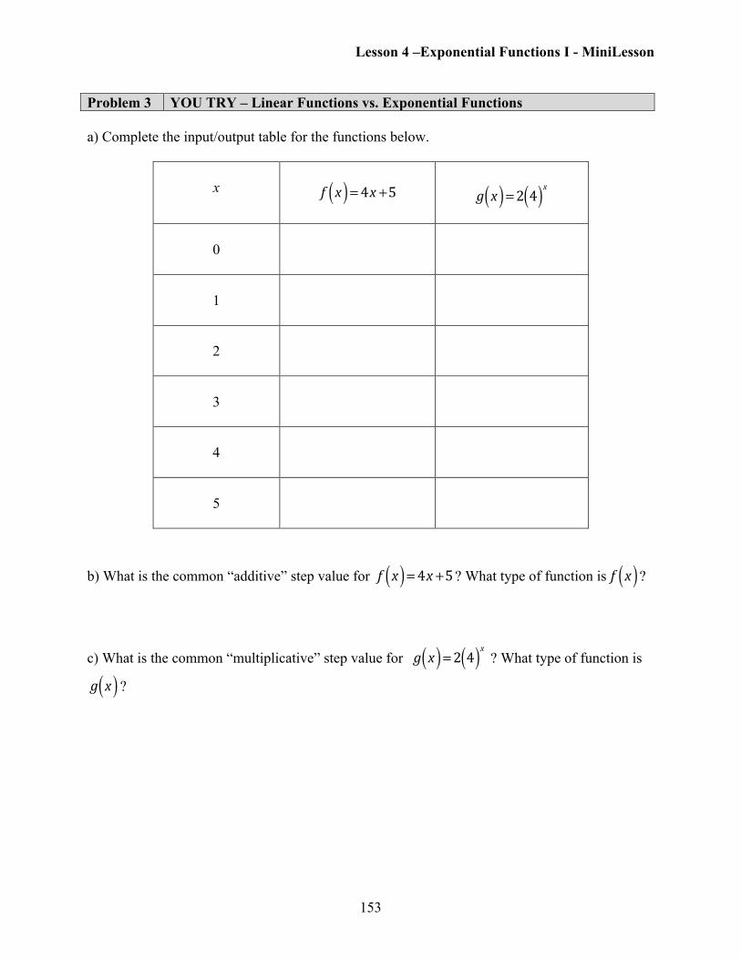
Problem 3 YOU TRY – Linear Functions vs. Exponential Functions a) Complete the input/output table for the functions below.

x

!!f x( ) = 4x +5

!!g x( ) =2 4( )x

0

1

2

3

4

5

b) What is the common “additive” step value for !!f x( ) = 4x +5? What type of function is!

f x( )?

c) What is the common “multiplicative” step value for !!g x( ) =2 4( )x ? What type of function is

!g x( ) ?


154

Are the Data Exponential?

To determine if an exponential function is the best model for a given data set, we calculate the

ratio,!!y2y1

, for each of the consecutive ordered pairs. If this ratio is approximately equal for each

of the consecutive ordered pairs, then an exponential function models the data best.

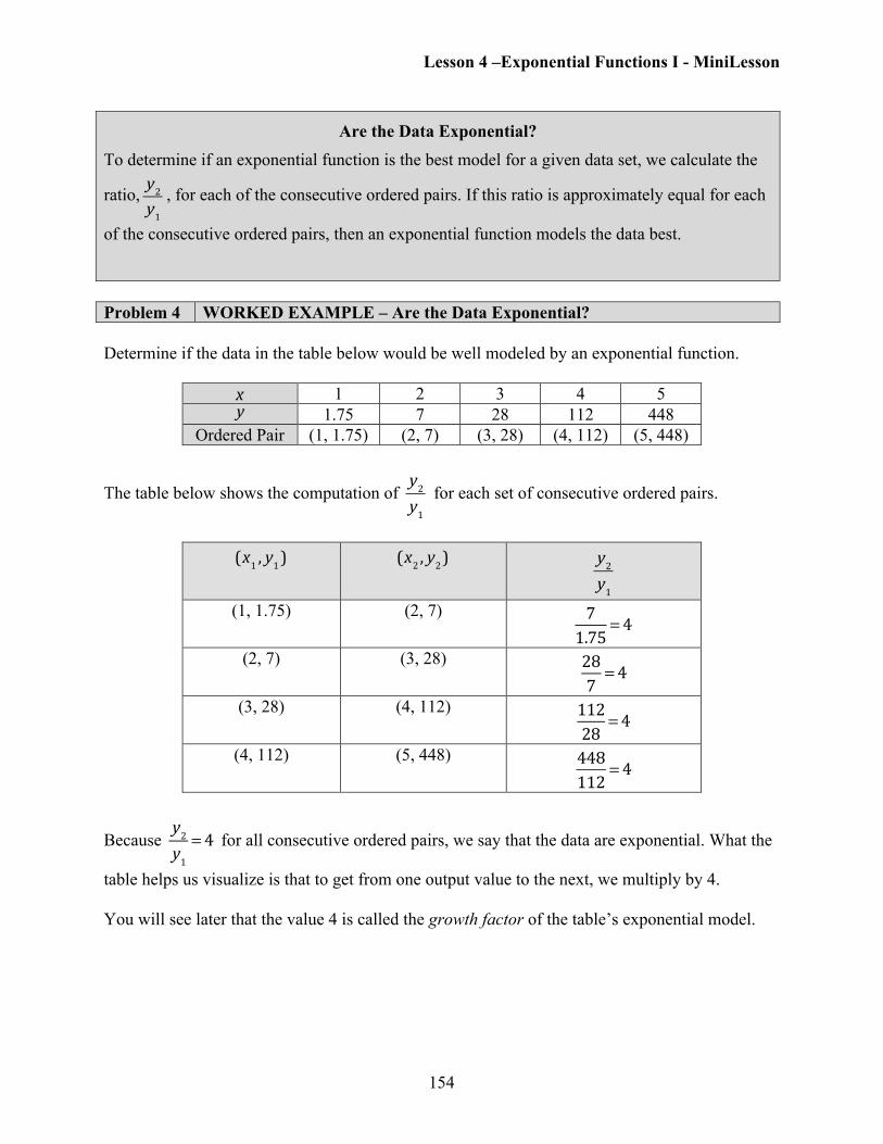
Problem 4 WORKED EXAMPLE – Are the Data Exponential? Determine if the data in the table below would be well modeled by an exponential function.

!x 1 2 3 4 5 !y 1.75 7 28 112 448

Ordered Pair (1, 1.75) (2, 7) (3, 28) (4, 112) (5, 448)

The table below shows the computation of !!y2y1

for each set of consecutive ordered pairs.

!!(x1 , y1) !!(x2 , y2)

!!y2y1

(1, 1.75) (2, 7)

!71.75 = 4

(2, 7) (3, 28)

!287 = 4

(3, 28) (4, 112)

!11228 = 4

(4, 112) (5, 448)

!448112 = 4

Because !!y2y1

= 4 for all consecutive ordered pairs, we say that the data are exponential. What the

table helps us visualize is that to get from one output value to the next, we multiply by 4. You will see later that the value 4 is called the growth factor of the table’s exponential model.


155

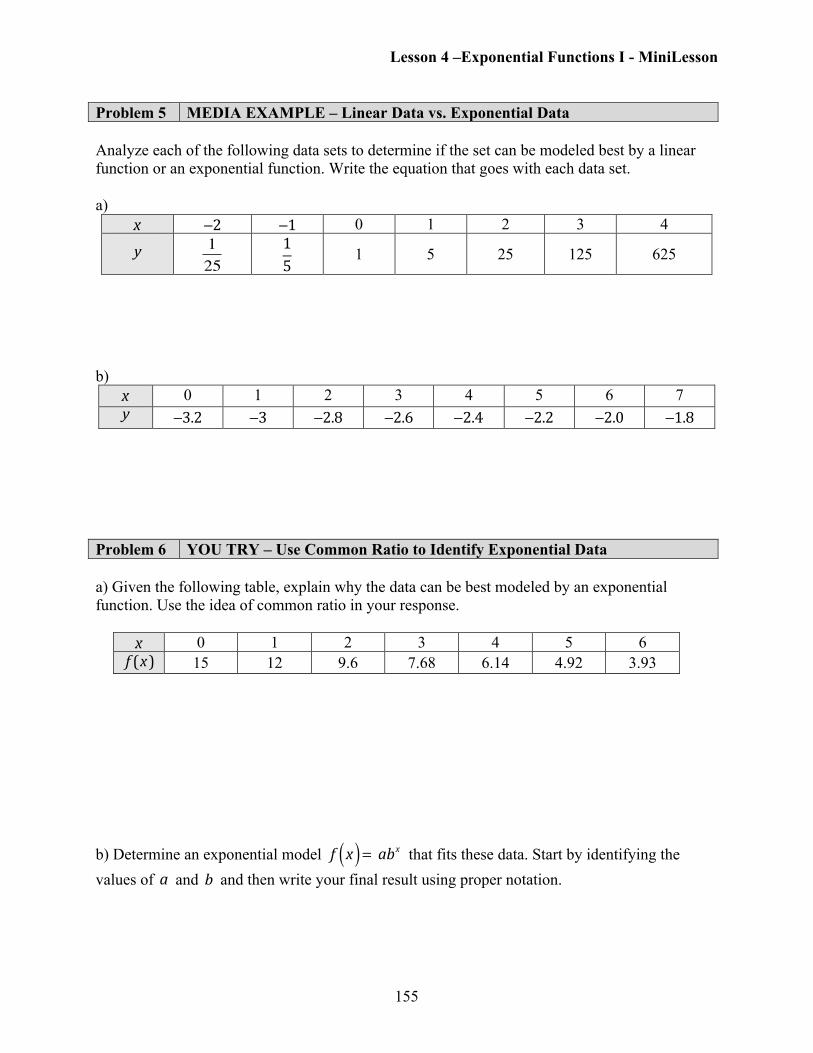
Problem 5 MEDIA EXAMPLE – Linear Data vs. Exponential Data Analyze each of the following data sets to determine if the set can be modeled best by a linear function or an exponential function. Write the equation that goes with each data set. a)

!x !−2 !−1 0 1 2 3 4

!y 125

15 1 5 25 125 625

b)

!x 0 1 2 3 4 5 6 7 !y !−3.2 !−3 !−2.8 !−2.6 !−2.4 !−2.2 !−2.0 !−1.8

Problem 6 YOU TRY – Use Common Ratio to Identify Exponential Data a) Given the following table, explain why the data can be best modeled by an exponential function. Use the idea of common ratio in your response.

!x 0 1 2 3 4 5 6 !!f (x) 15 12 9.6 7.68 6.14 4.92 3.93

b) Determine an exponential model !!f x( ) = !abx ! that fits these data. Start by identifying the values of !a and !b and then write your final result using proper notation.


156

Section 4.2 – Characteristics of Exponential Functions

Exponential Functions – General Form and Characteristics Exponential Functions are of the form !

f x( ) = abx where:

• !a is the initial value (also can be found by computing !!f 0( )). • !b is the base (!!b>0 and !!b≠1 ); also called the growth factor or decay factor.

• Input is in the exponent location.

• The graph of !f x( ) is in the shape of the letter “J” with vertical intercept !!(0, a) and base

!b (note that !b is the same as the common ratio from previous examples).

• If !!b>1 , the function is an exponential growth function, and the graph increases from left to right.

• If !!0! <b< !1 , the function is an exponential decay function, and the graph decreases from left to right.

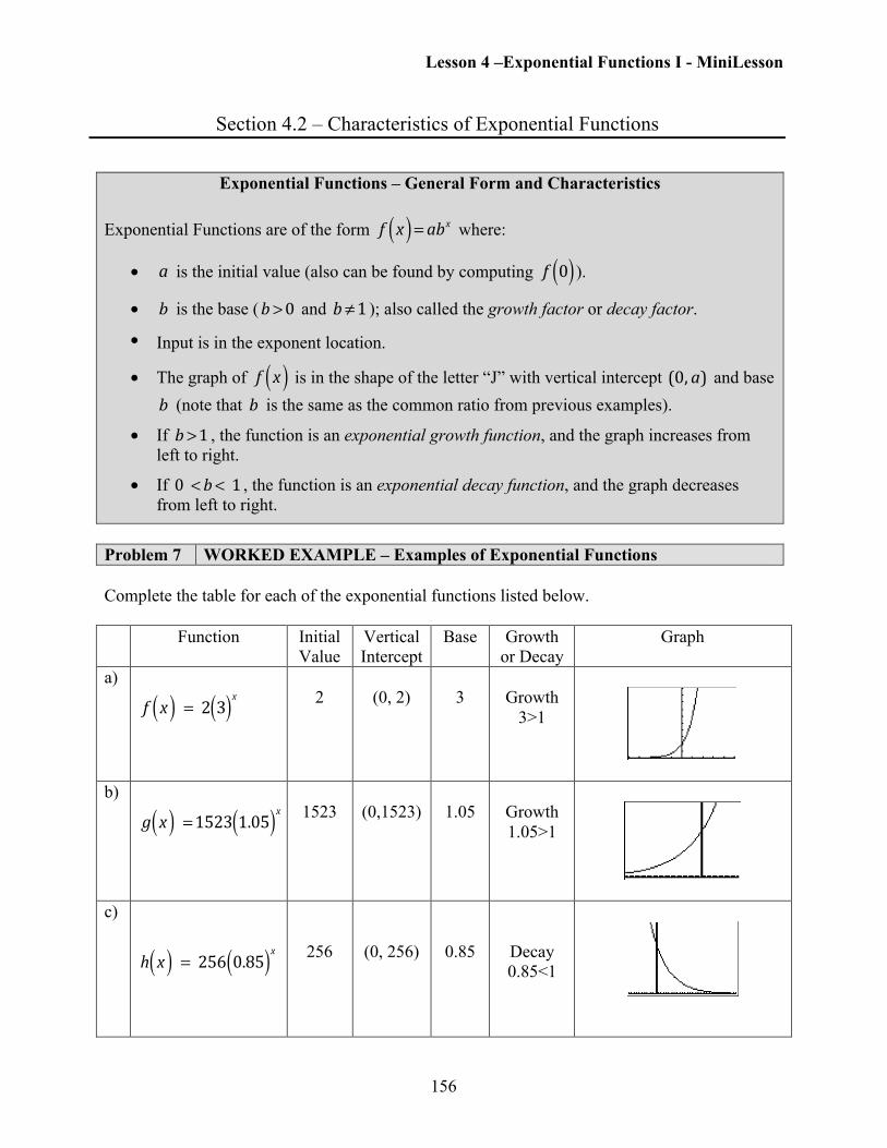
Problem 7 WORKED EXAMPLE – Examples of Exponential Functions Complete the table for each of the exponential functions listed below.

Function Initial Value

Vertical Intercept

Base Growth or Decay

Graph

a)

!!f x( ) ! = !2 3( )x !

2

(0, 2)

3

Growth

3>1

b)

!!g x( ) ! =1523 1.05( )x !

1523

(0,1523)

1.05

Growth 1.05>1

c)

!!h x( ) ! = !256 0.85( )x

256

(0, 256)

0.85

Decay 0.85<1


157

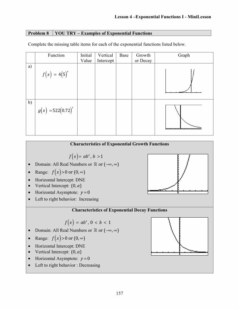
Problem 8 YOU TRY – Examples of Exponential Functions Complete the missing table items for each of the exponential functions listed below.

Function Initial Value

Vertical Intercept

Base Growth or Decay

Graph

a)

!!f x( ) ! = !4 5( )x !

b)

!!g x( ) ! =522 0.72( )x !

Characteristics of Exponential Growth Functions

!!f x( ) = !abx , !b! >1

• Domain: All Real Numbers or ! !!or!(−∞,∞) • Range: !!f x( ) >0!or!(0,∞)

• Horizontal Intercept: DNE • Vertical Intercept: !!(0, a) • Horizontal Asymptote: !!y =0 • Left to right behavior: Increasing

Characteristics of Exponential Decay Functions

!!f x( ) ! = !abx , !0! < !b! < !1

• Domain: All Real Numbers or ! !!or!(−∞,∞) • Range: !!f x( ) >0!or!(0,∞)

• Horizontal Intercept: DNE • Vertical Intercept: !!(0, a) • Horizontal Asymptote: !!y =0 • Left to right behavior : Decreasing


158

Problem 9 MEDIA EXAMPLE – Characteristics of Exponential Functions Complete the table below for each of the functions. Draw your graph by hand first, then confirm using your calculator and the window: X[-10..10], Y[0..500].

!!f x( ) =150 1.25( )x !!g x( ) =150 0.75( )x

Graph

Initial Value

Base

Domain

Range

Horizontal Intercept

Vertical Intercept

Horizontal Asymptote

Increasing or Decreasing


159

Problem 10 YOU TRY – Characteristics of Exponential Functions Complete the table below for each of the functions. Draw your graph by hand first, then confirm using your calculator and the window: X[-10..10], Y[0..500].

!!f x( ) =235 1.14( )x !!g x( ) =235 0.95( )x

Graph

Initial Value

Base

Domain

Range

Horizontal Intercept

Vertical Intercept

Horizontal Asymptote

Increasing or Decreasing


160

Section 4.3 – Solving Exponential Equations by Graphing

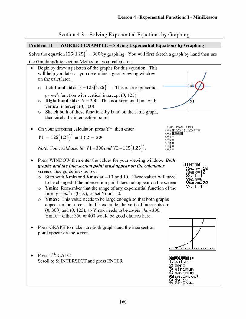
Problem 11 WORKED EXAMPLE – Solving Exponential Equations by Graphing

Solve the equation!!125 1.25( )x ! =300 by graphing. You will first sketch a graph by hand then use the Graphing/Intersection Method on your calculator. • Begin by drawing sketch of the graphs for this equation. This

will help you later as you determine a good viewing window on the calculator.

o Left hand side: !!Y =125 1.25( )x ! . This is an exponential growth function with vertical intercept (0, 125)

o Right hand side: Y = 300. This is a horizontal line with vertical intercept (0, 300).

o Sketch both of these functions by hand on the same graph, then circle the intersection point.

• On your graphing calculator, press Y= then enter

!!Y1! = !125 1.25( )x ! and !!Y2! = !300

Note: You could also let !!Y1=300 and !!Y2=125 1.25( )x .

• Press WINDOW then enter the values for your viewing window. Both graphs and the intersection point must appear on the calculator screen. See guidelines below. o Start with Xmin and Xmax at !−10 and 10. These values will need

to be changed if the intersection point does not appear on the screen. o Ymin: Remember that the range of any exponential function of the

form y = abx is (0, ∞), so set Ymin = 0. o Ymax: This value needs to be large enough so that both graphs

appear on the screen. In this example, the vertical intercepts are (0, 300) and (0, 125), so Ymax needs to be larger than 300. Ymax = either 350 or 400 would be good choices here.

• Press GRAPH to make sure both graphs and the intersection

point appear on the screen.

• Press 2nd>CALC

Scroll to 5: INTERSECT and press ENTER


161

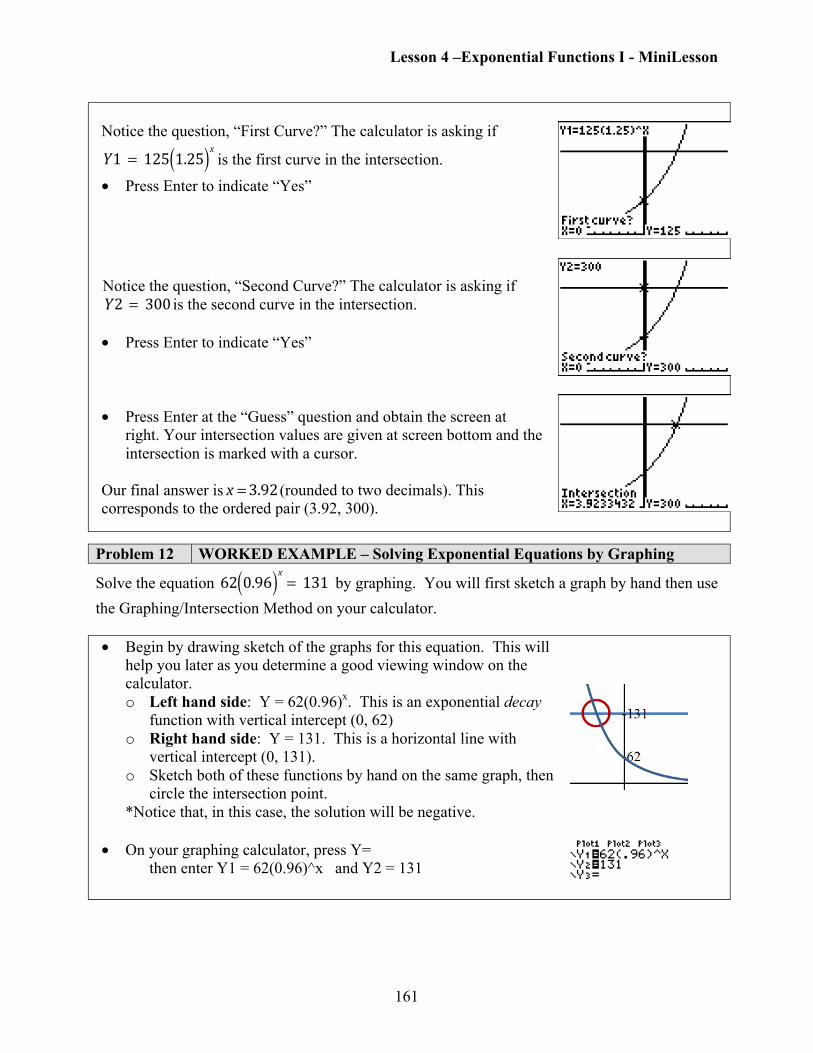
Notice the question, “First Curve?” The calculator is asking if

!!Y1! = !125 1.25( )x is the first curve in the intersection.

• Press Enter to indicate “Yes”

Notice the question, “Second Curve?” The calculator is asking if !!Y2! = !300 is the second curve in the intersection. • Press Enter to indicate “Yes”

• Press Enter at the “Guess” question and obtain the screen at

right. Your intersection values are given at screen bottom and the intersection is marked with a cursor.

Our final answer is!!x =3.92(rounded to two decimals). This corresponds to the ordered pair (3.92, 300).

Problem 12 WORKED EXAMPLE – Solving Exponential Equations by Graphing

Solve the equation !!62 0.96( )x = !131! by graphing. You will first sketch a graph by hand then use the Graphing/Intersection Method on your calculator. • Begin by drawing sketch of the graphs for this equation. This will

help you later as you determine a good viewing window on the calculator. o Left hand side: Y = 62(0.96)x. This is an exponential decay

function with vertical intercept (0, 62) o Right hand side: Y = 131. This is a horizontal line with

vertical intercept (0, 131). o Sketch both of these functions by hand on the same graph, then

circle the intersection point. *Notice that, in this case, the solution will be negative.

• On your graphing calculator, press Y= then enter Y1 = 62(0.96)^x and Y2 = 131


162

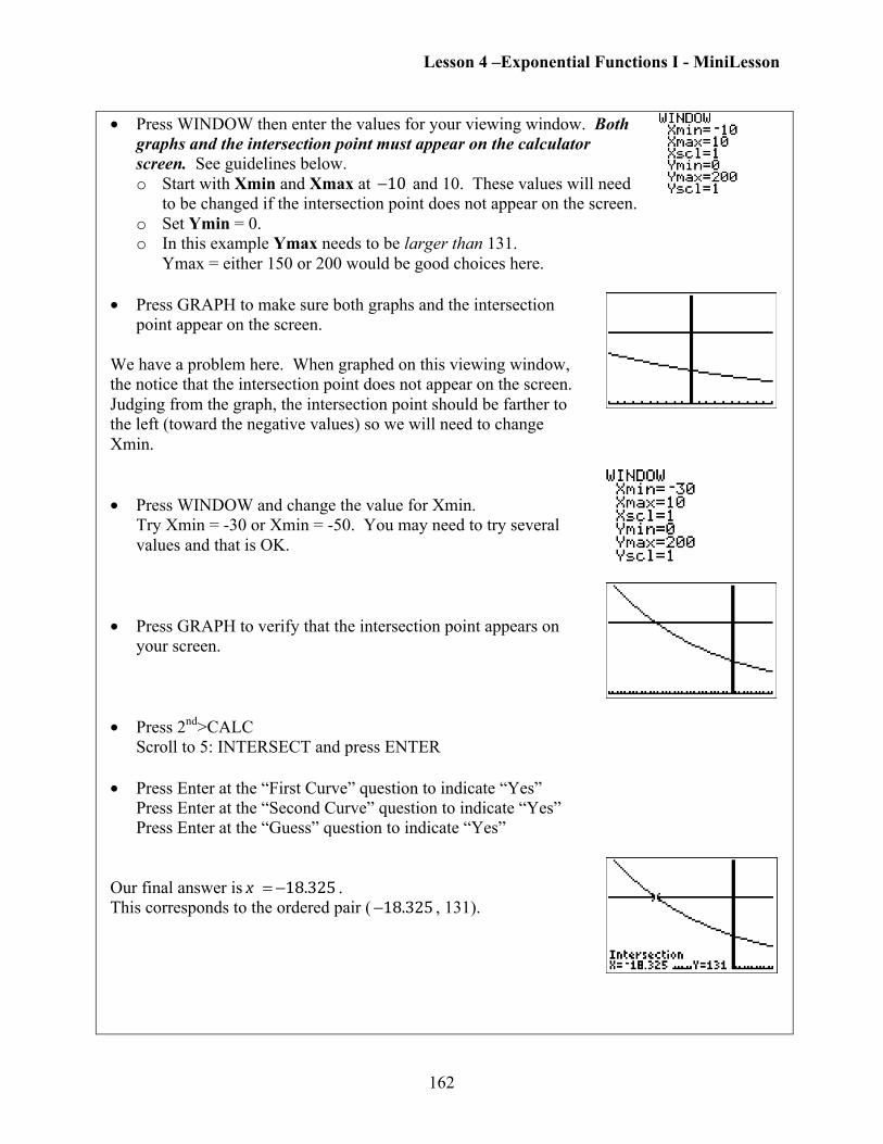
• Press WINDOW then enter the values for your viewing window. Both graphs and the intersection point must appear on the calculator screen. See guidelines below. o Start with Xmin and Xmax at !−10 and 10. These values will need

to be changed if the intersection point does not appear on the screen. o Set Ymin = 0. o In this example Ymax needs to be larger than 131.

Ymax = either 150 or 200 would be good choices here.

• Press GRAPH to make sure both graphs and the intersection

point appear on the screen. We have a problem here. When graphed on this viewing window, the notice that the intersection point does not appear on the screen. Judging from the graph, the intersection point should be farther to the left (toward the negative values) so we will need to change Xmin. • Press WINDOW and change the value for Xmin.

Try Xmin = -30 or Xmin = -50. You may need to try several values and that is OK.

• Press GRAPH to verify that the intersection point appears on

your screen.

• Press 2nd>CALC

Scroll to 5: INTERSECT and press ENTER

• Press Enter at the “First Curve” question to indicate “Yes” Press Enter at the “Second Curve” question to indicate “Yes” Press Enter at the “Guess” question to indicate “Yes”

Our final answer is!!x ! = −18.325 . This corresponds to the ordered pair (!−18.325 , 131).


163

GUIDELINES FOR SELECTING WINDOW VALUES FOR INTERSECTIONS While the steps for using the Graphing/Intersection Method are straightforward, choosing values for your window are not always easy. Here are some guidelines for choosing the edges of your window:

• Start by drawing a sketch of the graph by hand. This will help you visualize the situation, and will help you to determine the viewing window.

• The intersection of the equations MUST appear clearly in the window you select. Try to avoid intersections that appear just on the window’s edges, as these are hard to see and your calculator will often not process them correctly.

• When choosing values for x, start with the standard Xmin = -10 and Xmax = 10 UNLESS the problem is a real-world problem. In that case, start with Xmin=0 as negative values for a world problem are usually not important. If the values for Xmax need to be increased, choose 25, then 50, then 100 until the intersection of graphs is visible.

• When choosing values for y, start with Ymin = 0 unless negative values of Y are needed for some reason. For Ymax, make sure to choose a value so that all graphs and intercepts

appear on the screen. So, if solving something like!!234 1.23( )x = !1000 , then choose Ymax to be bigger than 1000 (say, 1200 or 1500). Otherwise the graph of !!y ! = !1000 will not appear.

• If the intersection does not appear in the window, then you will need to adjust your Xmin or Xmax settings. Try to change only one window setting at a time so you can clearly identify the effect of that change (i.e. make Xmin smaller OR make Xmax bigger but not both at once). Refer to your sketch and try to think about the functions you are working with and what they look like and use a systematic approach to making changes.

Problem 13 WORKED EXAMPLE – Choosing Window Values for Exponential

Equations The table below illustrates recommended window values to show important aspects of the given equations. Graph each one on your own calculator to verify the window choices below. Y1 is the left side of the equation and Y2 is the right side. Other window values will also work.

Equation Xmin Xmax Ymin Ymax

!!50=25(1.15)x -10 10 0 75

!!250=25(1.15)x -10 25 0 300

!!5=10(0.86)t -10 10 0 15

!!40=10(0.86)t -15 10 0 50

!!1500=1000(2.32)x -10 10 0 2000

!!400=1000(2.32)x -10 10 0 1100


164

Problem 14 MEDIA EXAMPLE – Solving Exponential Equations by Graphing In each situation below, use graphing to find the solution to the equation using the Graphing/Intersection Method described in this lesson. Fill in the missing blanks for each situation. Include a rough but accurate sketch of the graphs and intersection point. Mark and label the intersection. Round answers to two decimal places.

a) Solve !!50=25 1.15( )x Solution: x = ______________

Xmin = __________ Xmax = __________ Ymin = __________ Ymax = __________

b) Solve !!250=25 1.15( )x Solution: x = ______________


c) Solve !!5=10 0.86( )t Solution: t = ______________



165

d) Solve !!40=10 0.86( )t Solution: t = ______________


e) Solve !!1500=1000 2.32( )x Solution: x = ______________


e) Solve !!400=1000 2.32( )x Solution: x = ______________



166

Problem 15 YOU TRY – Solving Exponential Equations by Graphing

In each situation below, use graphing to find the solution to the equation using the Graphing/Intersection Method described in this lesson. Fill in the missing blanks for each situation. Include a rough but accurate sketch of the graphs and intersection point. Mark and label the intersection. Round answers to two decimal places.

a) Solve !!54 1.05( )x =250 Solution: x = ______________


b) Solve !!2340 0.82( )x =1250 Solution: x = ______________


c) Solve !!45! = !250 1.045( )x !!! Solution: x = ______________



167

Section 4.4 – Applications of Exponential Functions

Writing Exponential Function Models Use the following steps to help you write an exponential model for a given data set:

1. Identify the initial value. This is the “!a ” part of the exponential function!!f x( ) ! = !abx . To find !a , look for the output that goes with an input of 0.

2. Find the common ratio. This is the “!b ”part of the exponential function!!f x( ) ! = !abx . To find !b , make a fraction (ratio) of any two consecutive outputs (as long as the inputs are separated by exactly 1). Simplify this fraction and round as the problem indicates to obtain the value of !b .

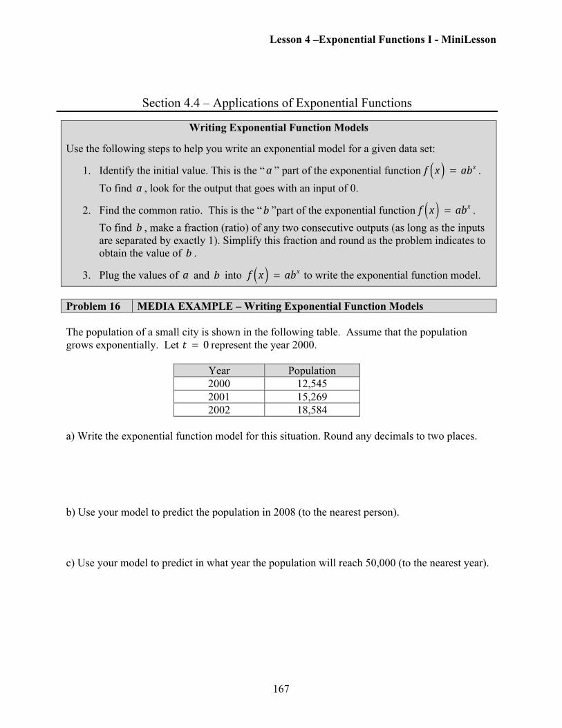
3. Plug the values of !a and !b into !!f x( ) ! = !abx to write the exponential function model. Problem 16 MEDIA EXAMPLE – Writing Exponential Function Models The population of a small city is shown in the following table. Assume that the population grows exponentially. Let !!t ! = !0 represent the year 2000.

Year Population 2000 12,545 2001 15,269 2002 18,584

a) Write the exponential function model for this situation. Round any decimals to two places. b) Use your model to predict the population in 2008 (to the nearest person). c) Use your model to predict in what year the population will reach 50,000 (to the nearest year).


168

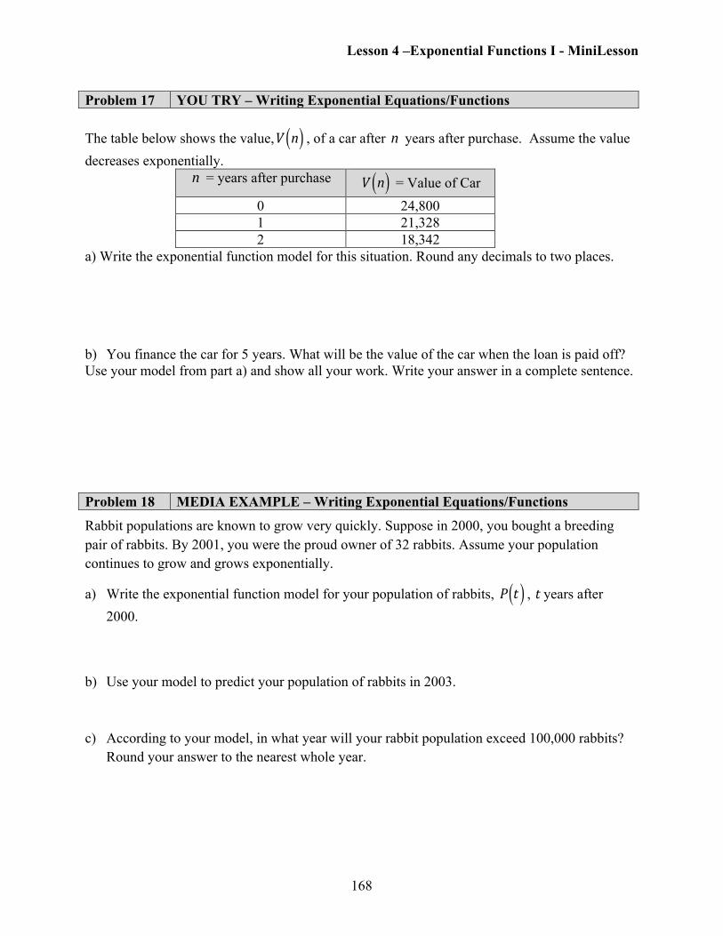
Problem 17 YOU TRY – Writing Exponential Equations/Functions The table below shows the value,!

V n( ) , of a car after !n years after purchase. Assume the value decreases exponentially.

!n = years after purchase !V n( ) = Value of Car

0 24,800 1 21,328 2 18,342

a) Write the exponential function model for this situation. Round any decimals to two places. b) You finance the car for 5 years. What will be the value of the car when the loan is paid off? Use your model from part a) and show all your work. Write your answer in a complete sentence. Problem 18 MEDIA EXAMPLE – Writing Exponential Equations/Functions

Rabbit populations are known to grow very quickly. Suppose in 2000, you bought a breeding pair of rabbits. By 2001, you were the proud owner of 32 rabbits. Assume your population continues to grow and grows exponentially.

a) Write the exponential function model for your population of rabbits, !P t( ) , !t years after

2000.

b) Use your model to predict your population of rabbits in 2003.

c) According to your model, in what year will your rabbit population exceed 100,000 rabbits? Round your answer to the nearest whole year.


169

Problem 19 YOU TRY – Writing Exponential Equations/Functions

In 2010, the population of Gilbert, AZ was about 208,000. By 2011, the population had grown to about 215,000. Assume that the population grows exponentially.

a) Write the exponential function model that expresses the population of Gilbert, !P t( ) , !t years

after 2010. Round numerical values to three decimals as needed.

b) Use your model to predict the population of Gilbert in 2014. Write your answer in a complete sentence.

c) Based on the model, in what year will the population of Gilbert reach 300,000? Round your answer to the nearest whole year. Write your answer in a complete sentence.

Problem 20 YOU TRY – Applications of Exponential Functions

One 8-oz cup of coffee contains about 100 mg of caffeine. The function !!A x( ) ! = !100 0.88( )x !gives the amount of caffeine (in mg) remaining in the body !x hours after drinking an 8-oz cup of coffee. Show all work. Write answers in complete sentences. Round numerical results to two places.

a) Identify the vertical intercept of this function. Interpret its meaning in this situation. b) How much caffeine remains in the body 8 hours after drinking a cup of coffee? c) How long will it take the body to metabolize half of the caffeine from one 8-oz cup of coffee? (i.e. How long until only 50 mg of caffeine remains in the body?)

Lesson 4 –Exponential Functions I · ... then an exponential function models the data best. ......

Documents

Transcript of Lesson 4 –Exponential Functions I · ... then an exponential function models the data best. ......