Lesson 2: Entering Excel Formulas and Formatting … · Lesson 2: Entering Excel Formulas and...

EXCEL 2007 Tutorial Lesson 2 2010/2011

Lesson 2: Entering Excel Formulas and Formatting Data

Lesson 1 familiarized you with the Excel 2007 window, taught you how to move around the

window, and how to enter data. A major strength of Excel is that you can perform mathematical

calculations and format your data. In this lesson, you learn how to perform basic mathematical

calculations and how to format text and numerical data. To start this lesson, open Excel.

Set the Enter Key Direction

In Microsoft Excel, you can specify the direction the cursor moves when you press the Enter key.

In the exercises that follow, the cursor must move down one cell when you press Enter. You can

use the Direction box in the Excel Options pane to set the cursor to move up, down, left, right, or

not at all. Perform the steps that follow to set the cursor to move down when you press the Enter

key.

1. Click the Microsoft Office button. A menu appears.

2. Click Excel Options in the lower-right corner. The Excel Options pane appears.


3. Click Advanced.

4. If the check box next to After Pressing Enter Move Selection is not checked, click the

box to check it.

5. If Down does not appear in the Direction box, click the down arrow next to the Direction

box and then click Down.

6. Click OK. Excel sets the Enter direction to down.

Perform Mathematical Calculations

In Microsoft Excel, you can enter numbers and mathematical formulas into cells. Whether you

enter a number or a formula, you can reference the cell when you perform mathematical

calculations such as addition, subtraction, multiplication, or division. When entering a

mathematical formula, precede the formula with an equal sign. Use the following to indicate the

type of calculation you wish to perform:

+ Addition

- Subtraction

* Multiplication

/ Division

^ Exponential


In the following exercises, you practice some of the methods you can use to move around a

worksheet and you learn how to perform mathematical calculations. Refer to Lesson 1 to learn

more about moving around a worksheet.

EXERCISE 1

Addition

1. Type Add in cell A1.

2. Press Enter. Excel moves down one cell.

3. Type 1 in cell A2.


5. Type 1 in cell A3.


7. Type =A2+A3 in cell A4.

8. Click the check mark on the Formula bar. Excel adds cell A1 to cell A2 and displays the

result in cell A4. The formula displays on the Formula bar.

Note: Clicking the check mark on the Formula bar is similar to pressing Enter. Excel records

your entry but does not move to the next cell.

Subtraction


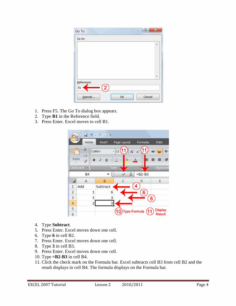
1. Press F5. The Go To dialog box appears.

2. Type B1 in the Reference field.

3. Press Enter. Excel moves to cell B1.

4. Type Subtract.


6. Type 6 in cell B2.


8. Type 3 in cell B3.


10. Type =B2-B3 in cell B4.

11. Click the check mark on the Formula bar. Excel subtracts cell B3 from cell B2 and the

result displays in cell B4. The formula displays on the Formula bar.


Multiplication

1. Hold down the Ctrl key while you press "g" (Ctrl+g). The Go To dialog box appears.

2. Type C1 in the Reference field.

3. Press Enter. Excel moves to cell C1

4. Type Multiply.


6. Type 2 in cell C2.


8. Type 3 in cell C3.


10. Type =C2*C3 in cell C4.

11. Click the check mark on the Formula bar. Excel multiplies C1 by cell C2 and displays the

result in cell C3. The formula displays on the Formula bar.

Division

1. Press F5.

2. Type D1 in the Reference field.

3. Press Enter. Excel moves to cell D1.

4. Type Divide.


6. Type 6 in cell D2.


8. Type 3 in cell D3.


10. Type =D2/D3 in cell D4.

11. Click the check mark on the Formula bar. Excel divides cell D2 by cell D3 and displays

the result in cell D4. The formula displays on the Formula bar.

When creating formulas, you can reference cells and include numbers. All of the following

formulas are valid:

=A2/B2

=A1+12-B3

=A2*B2+12

=24+53

AutoSum

You can use the AutoSum button on the Home tab to automatically add a column or row of

numbers. When you press the AutoSum button , Excel selects the numbers it thinks you want

to add. If you then click the check mark on the Formula bar or press the Enter key, Excel adds


the numbers. If Excel's guess as to which numbers you want to add is wrong, you can select the

cells you want.

EXERCISE 2

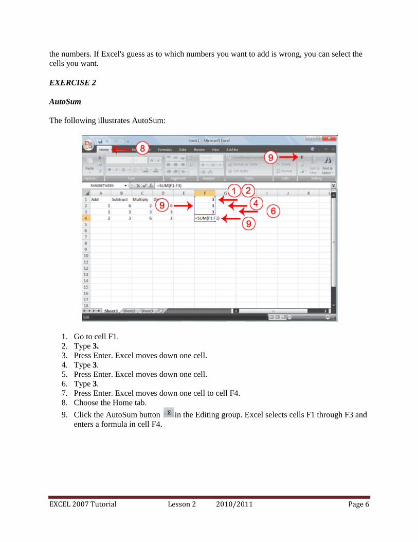
AutoSum

The following illustrates AutoSum:

1. Go to cell F1.

2. Type 3.


4. Type 3.


6. Type 3.

7. Press Enter. Excel moves down one cell to cell F4.

8. Choose the Home tab.

9. Click the AutoSum button in the Editing group. Excel selects cells F1 through F3 and

enters a formula in cell F4.


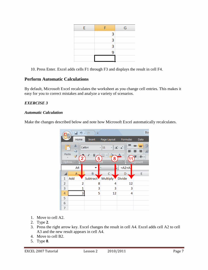
10. Press Enter. Excel adds cells F1 through F3 and displays the result in cell F4.

Perform Automatic Calculations

By default, Microsoft Excel recalculates the worksheet as you change cell entries. This makes it

easy for you to correct mistakes and analyze a variety of scenarios.

EXERCISE 3

Automatic Calculation

Make the changes described below and note how Microsoft Excel automatically recalculates.

1. Move to cell A2.

2. Type 2.

3. Press the right arrow key. Excel changes the result in cell A4. Excel adds cell A2 to cell

A3 and the new result appears in cell A4.

4. Move to cell B2.

5. Type 8.


6. Press the right arrow key. Excel subtracts cell B3 from cell B3 and the new result

appears in cell B4.

7. Move to cell C2.

8. Type 4.

9. Press the right arrow key. Excel multiplies cell C2 by cell C3 and the new result appears

in cell C4.

10. Move to cell D2.

11. Type 12.

12. Press the Enter key. Excel divides cell D2 by cell D3 and the new result appears in cell

D4.

Align Cell Entries

When you type text into a cell, by default your entry aligns with the left side of the cell. When

you type numbers into a cell, by default your entry aligns with the right side of the cell. You can

change the cell alignment. You can center, left-align, or right-align any cell entry. Look at cells

A1 to D1. Note that they are aligned with the left side of the cell.

EXERCISE 4

Center

To center cells A1 to D1:

1. Select cells A1 to D1.


3. Click the Center button in the Alignment group. Excel centers each cell's content.


Left-Align

To left-align cells A1 to D1:

1. Select cells A1 to D1.


3. Click the Align Text Left button in the Alignment group. Excel left-aligns each cell's

content.

Right-Align

To right-align cells A1 to D1:

1. Select cells A1 to D1. Click in cell A1.


3. Click the Align Text Right button. Excel right-aligns the cell's content.

4. Click anywhere on your worksheet to clear the highlighting.


Note: You can also change the alignment of cells with numbers in them by using the alignment

buttons.

Perform Advanced Mathematical Calculations

When you perform mathematical calculations in Excel, be careful of precedence. Calculations

are performed from left to right, with multiplication and division performed before addition and

subtraction.

EXERCISE 5

Advanced Calculations

1. Move to cell A7.

2. Type =3+3+12/2*4.

3. Press Enter.

Note: Microsoft Excel divides 12 by 2, multiplies the answer by 4, adds 3, and then adds another

3. The answer, 30, displays in cell A7.

To change the order of calculation, use parentheses. Microsoft Excel calculates the information

in parentheses first.

1. Double-click in cell A7.

2. Edit the cell to read =(3+3+12)/2*4.

3. Press Enter.

Note: Microsoft Excel adds 3 plus 3 plus 12, divides the answer by 2, and then multiplies the

result by 4. The answer, 36, displays in cell A7.

Copy, Cut, Paste, and Cell Addressing

In Excel, you can copy data from one area of a worksheet and place the data you copied

anywhere in the same or another worksheet. In other words, after you type information into a


worksheet, if you want to place the same information somewhere else, you do not have to retype

the information. You simple copy it and then paste it in the new location.

You can use Excel's Cut feature to remove information from a worksheet. Then you can use the

Paste feature to place the information you cut anywhere in the same or another worksheet. In

other words, you can move information from one place in a worksheet to another place in the

same or different worksheet by using the Cut and Paste features.

Microsoft Excel records cell addresses in formulas in three different ways, called absolute,

relative, and mixed. The way a formula is recorded is important when you copy it. With relative

cell addressing, when you copy a formula from one area of the worksheet to another, Excel

records the position of the cell relative to the cell that originally contained the formula. With

absolute cell addressing, when you copy a formula from one area of the worksheet to another,

Excel references the same cells, no matter where you copy the formula. You can use mixed cell

addressing to keep the row constant while the column changes, or vice versa. The following

exercises demonstrate.

EXERCISE 6

Copy, Cut, Paste, and Cell Addressing

1. Move to cell A9.

2. Type 1. Press Enter. Excel moves down one cell.



5. Move to cell B9.




In addition to typing a formula as you did in Lesson 1, you can also enter formulas by using

Point mode. When you are in Point mode, you can enter a formula either by clicking on a cell or

by using the arrow keys.

1. Move to cell A12.

2. Type =.

3. Use the up arrow key to move to cell A9.

4. Type +.


6. Type +.


8. Click the check mark on the Formula bar. Look at the Formula bar. Note that the formula

you entered is displayed there.


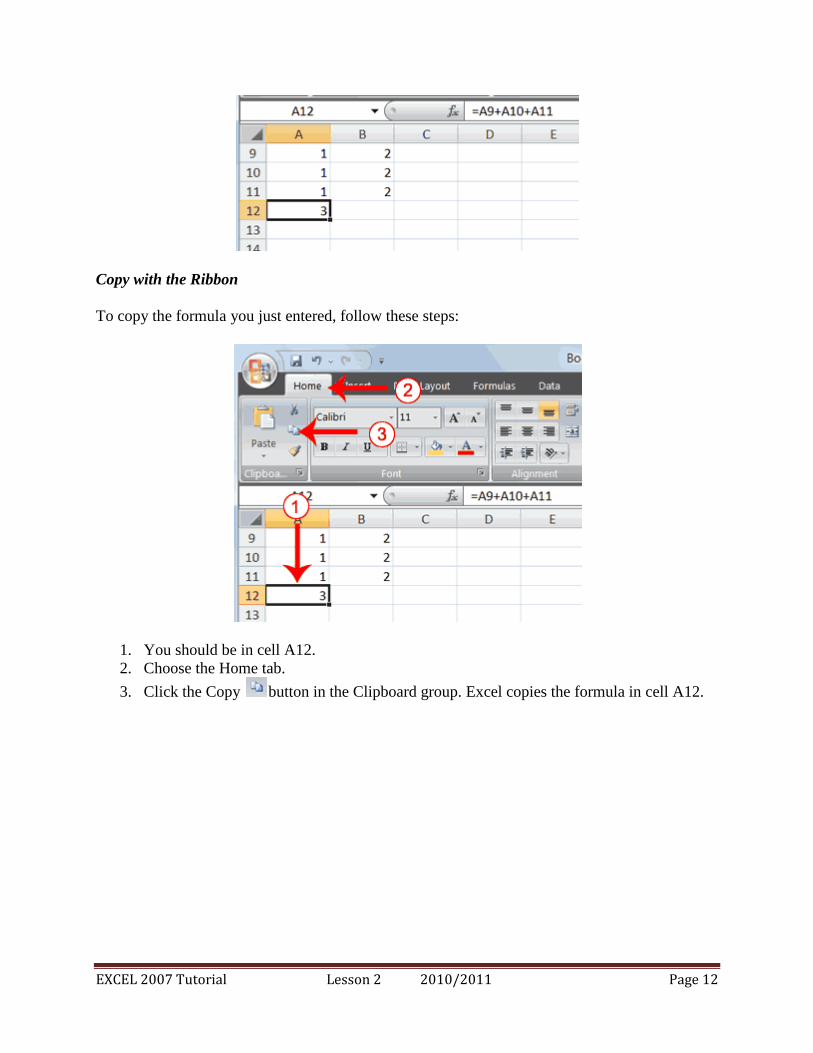
Copy with the Ribbon

To copy the formula you just entered, follow these steps:

1. You should be in cell A12.


3. Click the Copy button in the Clipboard group. Excel copies the formula in cell A12.


4. Press the right arrow key once to move to cell B12.

5. Click the Paste button in the Clipboard group. Excel pastes the formula in cell A12

into cell B12.

6. Press the Esc key to exit the Copy mode.

Compare the formula in cell A12 with the formula in cell B12 (while in the respective cell, look

at the Formula bar). The formulas are the same except that the formula in cell A12 sums the

entries in column A and the formula in cell B12 sums the entries in column B. The formula was

copied in a relative fashion.

Before proceeding with the next part of the exercise, you must copy the information in cells A7

to B9 to cells C7 to D9. This time you will copy by using the Mini toolbar.


Copy with the Mini Toolbar

1. Select cells A9 to B11. Move to cell A9. Press the Shift key. While holding down the

Shift key , press the down arrow key twice. Press the right arrow key once. Excel

highlights A9 to B11.

2. Right-click. A context menu and a Mini toolbar appear.

3. Click Copy, which is located on the context menu. Excel copies the information in cells

A9 to B11.

4. Move to cell C9.

5. Right-click. A context menu appears.

6. Click Paste. Excel copies the contents of cells A9 to B11 to cells C9 to C11.


7. Press Esc to exit Copy mode.

Absolute Cell Addressing

You make a cell address an absolute cell address by placing a dollar sign in front of the row and

column identifiers. You can do this automatically by using the F4 key. To illustrate:

1. Move to cell C12.

2. Type =.

3. Click cell C9.

4. Press F4. Dollar signs appear before the C and the 9.

5. Type +.

6. Click cell C10.


8. Type +.

9. Click cell C11.


11. Click the check mark on the formula bar. Excel records the formula in cell C12.

Copy and Paste with Keyboard Shortcuts

Keyboard shortcuts are key combinations that enable you to perform tasks by using the

keyboard. Generally, you press and hold down a key while pressing a letter. For example, Ctrl+c

means you should press and hold down the Ctrl key while pressing "c." This tutorial notates key

combinations as follows:

Press Ctrl+c.

Now copy the formula from C12 to D12. This time, copy by using keyboard shortcuts..

1. Move to cell C12.

2. Hold down the Ctrl key while you press "c" (Ctrl+c). Excel copies the contents of cell

C12.

3. Press the right arrow once. Excel moves to D12.

4. Hold down the Ctrl key while you press "v" (Ctrl+v). Excel pastes the contents of cell

C12 into cell D12.


5. Press Esc to exit the Copy mode.

Compare the formula in cell C12 with the formula in cell D12 (while in the respective cell, look

at the Formula bar). The formulas are exactly the same. Excel copied the formula from cell C12

to cell D12. Excel copied the formula in an absolute fashion. Both formulas sum column C.

Mixed Cell Addressing

You use mixed cell addressing to reference a cell when you want to copy part of it absolute and

part relative. For example, the row can be absolute and the column relative. You can use the F4

key to create a mixed cell reference.

1. Move to cell E1.

2. Type =.

3. Press the up arrow key once.

4. Press F4.

5. Press F4 again. Note that the column is relative and the row is absolute.

6. Press F4 again. Note that the column is absolute and the row is relative.

7. Press Esc.

Cut and Paste

You can move data from one area of a worksheet to another.


1. Select cells D9 to D12


3. Click the Cut button.

4. Move to cell G1.


5. Click the Paste button . Excel moves the contents of cells D9 to D12 to cells G1 to

G4.

The keyboard shortcut for Cut is Ctrl+x. The steps for cutting and pasting with a keyboard

shortcut are:

1. Select the cells you want to cut and paste.

2. Press Ctrl+x.

3. Move to the upper-left corner of the block of cells into which you want to paste.

4. Press Ctrl+v. Excel cuts and pastes the cells you selected.

Insert and Delete Columns and Rows

You can insert and delete columns and rows. When you delete a column, you delete everything

in the column from the top of the worksheet to the bottom of the worksheet. When you delete a

row, you delete the entire row from left to right. Inserting a column or row inserts a completely

new column or row.

EXERCISE 7

Insert and Delete Columns and Rows

To delete columns F and G:

1. Click the column F indicator and drag to column G.


2. Click the down arrow next to Delete in the Cells group. A menu appears.

3. Click Delete Sheet Columns. Excel deletes the columns you selected.

4. Click anywhere on the worksheet to remove your selection.

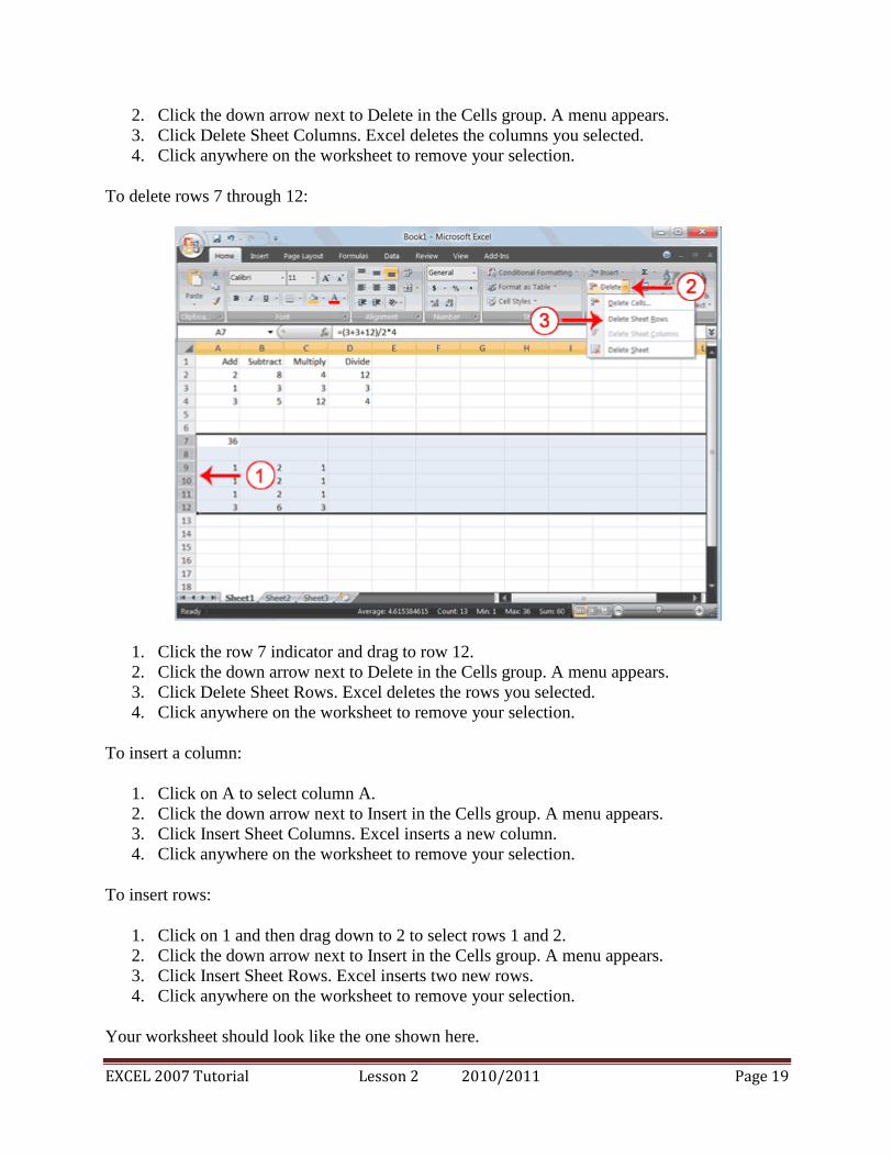
To delete rows 7 through 12:

1. Click the row 7 indicator and drag to row 12.

2. Click the down arrow next to Delete in the Cells group. A menu appears.

3. Click Delete Sheet Rows. Excel deletes the rows you selected.


To insert a column:

1. Click on A to select column A.

2. Click the down arrow next to Insert in the Cells group. A menu appears.

3. Click Insert Sheet Columns. Excel inserts a new column.


To insert rows:

1. Click on 1 and then drag down to 2 to select rows 1 and 2.

2. Click the down arrow next to Insert in the Cells group. A menu appears.

3. Click Insert Sheet Rows. Excel inserts two new rows.


Your worksheet should look like the one shown here.


Create Borders

You can use borders to make entries in your Excel worksheet stand out. You can choose from

several types of borders. When you press the down arrow next to the Border button , a

menu appears. By making the proper selection from the menu, you can place a border on the top,

bottom, left, or right side of the selected cells; on all sides; or around the outside border. You can

have a thick outside border or a border with a single-line top and a double-line bottom.

Accountants usually place a single underline above a final number and a double underline below.

The following illustrates:

EXERCISE 8

Create Borders

1. Select cells B6 to E6.



3. Click the down arrow next to the Borders button . A menu appears.

4. Click Top and Double Bottom Border. Excel adds the border you chose to the selected

cells.


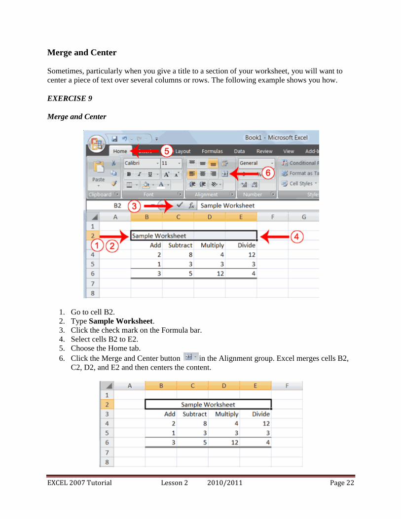
Merge and Center

Sometimes, particularly when you give a title to a section of your worksheet, you will want to

center a piece of text over several columns or rows. The following example shows you how.

EXERCISE 9

Merge and Center

1. Go to cell B2.

2. Type Sample Worksheet.

3. Click the check mark on the Formula bar.



6. Click the Merge and Center button in the Alignment group. Excel merges cells B2,

C2, D2, and E2 and then centers the content.


Note: To unmerge cells:

1. Select the cell you want to unmerge.


3. Click the down arrow next to the Merge and Center button. A menu appears.

4. Click Unmerge Cells. Excel unmerges the cells.

Add Background Color

To make a section of your worksheet stand out, you can add background color to a cell or group

of cells.

EXERCISE 10

Add Background Color



3. Click the down arrow next to the Fill Color button .

4. Click the color dark blue. Excel places a dark blue background in the cells you selected.


Change the Font, Font Size, and Font Color

A font is a set of characters represented in a single typeface. Each character within a font is

created by using the same basic style. Excel provides many different fonts from which you can

choose. The size of a font is measured in points. There are 72 points to an inch. The number of

points assigned to a font is based on the distance from the top to the bottom of its longest

character. You can change the Font, Font Size, and Font Color of the data you enter into Excel.

EXERCISE 11

Change the Font




3. Click the down arrow next to the Font box. A list of fonts appears. As you scroll down

the list of fonts, Excel provides a preview of the font in the cell you selected.

4. Find and click Times New Roman in the Font box. Note: If Times New Roman is your

default font, click another font. Excel changes the font in the selected cells.

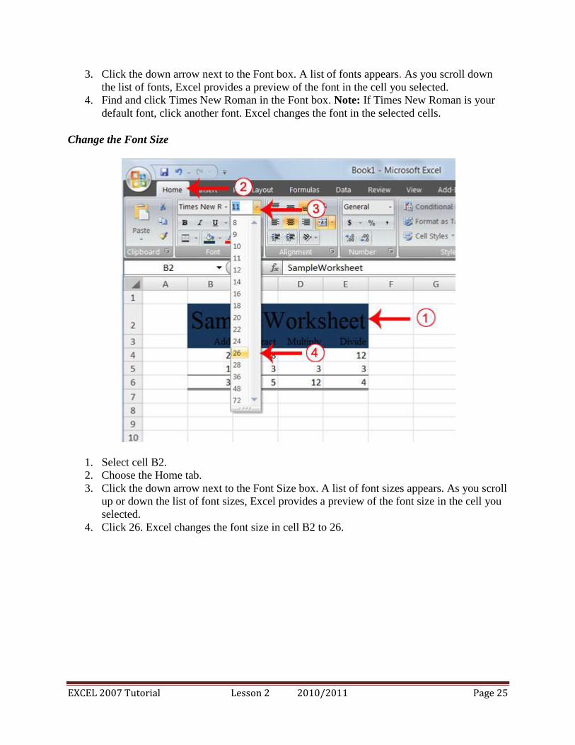
Change the Font Size

1. Select cell B2.


3. Click the down arrow next to the Font Size box. A list of font sizes appears. As you scroll

up or down the list of font sizes, Excel provides a preview of the font size in the cell you

selected.

4. Click 26. Excel changes the font size in cell B2 to 26.


Change the Font Color



3. Click the down arrow next to the Font Color button .

4. Click on the color white. Your font color changes to white.

Your worksheet should look like the one shown here.

Move to a New Worksheet

In Microsoft Excel, each workbook is made up of several worksheets. Each worksheet has a tab.

By default, a workbook has three sheets and they are named sequentially, starting with Sheet1.


The name of the worksheet appears on the tab. Before moving to the next topic, move to a new

worksheet. The exercise that follows shows you how.

EXERCISE 12

Move to a New Worksheet

Click Sheet2 in the lower-left corner of the screen. Excel moves to Sheet2.

Bold, Italicize, and Underline

When creating an Excel worksheet, you may want to emphasize the contents of cells by bolding,

italicizing, and/or underlining. You can easily bold, italicize, or underline text with Microsoft

Excel. You can also combine these features—in other words, you can bold, italicize, and

underline a single piece of text.

In the exercises that follow, you will learn different methods you can use to bold, italicize, and

underline.

EXERCISE 13

Bold with the Ribbon

1. Type Bold in cell A1.


2. Click the check mark located on the Formula bar.


4. Click the Bold button . Excel bolds the contents of the cell.

5. Click the Bold button again if you wish to remove the bold.

Italicize with the Ribbon

1. Type Italic in cell B1.



4. Click the Italic button . Excel italicizes the contents of the cell.

5. Click the Italic button again if you wish to remove the italic.

Underline with the Ribbon

Microsoft Excel provides two types of underlines. The exercises that follow illustrate them.

Single Underline:


1. Type Underline in cell C1.



4. Click the Underline button . Excel underlines the contents of the cell.

5. Click the Underline button again if you wish to remove the underline.

Double Underline

1. Type Underline in cell D1.



4. Click the down arrow next to the Underline button and then click Double Underline.

Excel double-underlines the contents of the cell. Note that the Underline button changes

to the button shown here , a D with a double underline under it. Then next time you

click the Underline button, you will get a double underline. If you want a single

underline, click the down arrow next to the Double Underline button and then

choose Underline.

5. Click the double underline button again if you wish to remove the double underline.

Bold, Underline, and Italicize

1. Type All three in cell E1.



4. Click the Bold button . Excel bolds the cell contents.

5. Click the Italic button . Excel italicizes the cell contents.

6. Click the Underline button . Excel underlines the cell contents.


Alternate Method: Bold with Shortcut Keys

1. Type Bold in cell A2.


3. Hold down the Ctrl key while pressing "b" (Ctrl+b). Excel bolds the contents of the cell.

4. Press Ctrl+b again if you wish to remove the bolding.

Alternate Method: Italicize with Shortcut Keys

1. Type Italic in cell B2. Note: Because you previously entered the word Italic in column

B, Excel may enter the word in the cell automatically after you type the letter I. Excel

does this to speed up your data entry.


3. Hold down the Ctrl key while pressing "i" (Ctrl+i). Excel italicizes the contents of the

cell.

4. Press Ctrl+i again if you wish to remove the italic formatting.

Alternate Method: Underline with Shortcut Keys

1. Type Underline in cell C2.


3. Hold down the Ctrl key while pressing "u" (Ctrl+u). Excel applies a single underline to

the cell contents.

4. Press Ctrl+u again if you wish to remove the underline.

Bold, Italicize, and Underline with Shortcut Keys

1. Type All three in cell D2.


3. Hold down the Ctrl key while pressing "b" (Ctrl+b). Excel bolds the cell contents.

4. Hold down the Ctrl key while pressing "i" (Ctrl+i). Excel italicizes the cell contents.

5. Hold down the Ctrl key while pressing "u" (Ctrl+u). Excel applies a single underline to

the cell contents.

Work with Long Text

Whenever you type text that is too long to fit into a cell, Microsoft Excel attempts to display all

the text. It left-aligns the text regardless of the alignment you have assigned to it, and it borrows

space from the blank cells to the right. However, a long text entry will never write over cells that

already contain entries—instead, the cells that contain entries cut off the long text. The following

exercise illustrates this.


EXERCISE 14

Work with Long Text

1. Move to cell A6.

2. Type Now is the time for all good men to go to the aid of their army.

3. Press Enter. Everything that does not fit into cell A6 spills over into the adjacent cell.

4. Move to cell B6.

5. Type Test.

6. Press Enter. Excel cuts off the entry in cell A6.

7. Move to cell A6.

8. Look at the Formula bar. The text is still in the cell.

Change A Column's Width

You can increase column widths. Increasing the column width enables you to see the long text.


EXERCISE 15

Change Column Width

1. Make sure you are in any cell under column A.


3. Click the down arrow next to Format in the Cells group.

4. Click Column Width. The Column Width dialog box appears.

5. Type 55 in the Column Width field.

6. Click OK. Column A is set to a width of 55. You should now be able to see all of the text.

Change a Column Width by Dragging

You can also change the column width with the cursor.

1. Place the mouse pointer on the line between the B and C column headings. The mouse

pointer should look like the one displayed here , with two arrows.

2. Move your mouse to the right while holding down the left mouse button. The width

indicator appears on the screen.

3. Release the left mouse button when the width indicator shows approximately 20. Excel

increases the column width to 20.


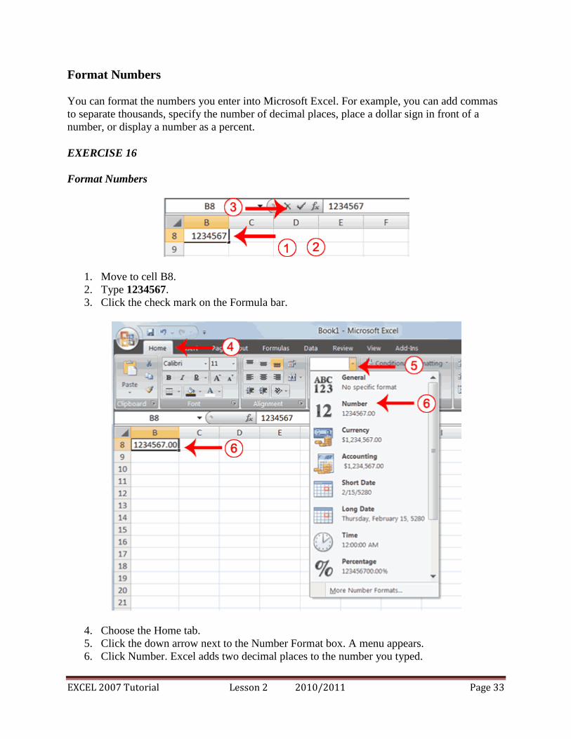
Format Numbers

You can format the numbers you enter into Microsoft Excel. For example, you can add commas

to separate thousands, specify the number of decimal places, place a dollar sign in front of a

number, or display a number as a percent.

EXERCISE 16

Format Numbers

1. Move to cell B8.

2. Type 1234567.

3. Click the check mark on the Formula bar.


5. Click the down arrow next to the Number Format box. A menu appears.

6. Click Number. Excel adds two decimal places to the number you typed.


7. Click the Comma Style button . Excel separates thousands with a comma.

8. Click the Accounting Number Format button . Excel adds a dollar sign to your

number.

9. Click twice on the Increase Decimal button to change the number format to four

decimal places.

10. Click the Decrease Decimal button if you wish to decrease the number of decimal

places.

Change a decimal to a percent.

1. Move to cell B9.

2. Type .35 (note the decimal point).

3. Click the check mark on the formula bar.



5. Click the Percent Style button . Excel turns the decimal to a percent.

This is the end of Lesson 2. You can save and close your file. See Lesson 1 to learn how to save

and close a file.

Lesson 2: Entering Excel Formulas and Formatting … · Lesson 2: Entering Excel Formulas and...

Documents

Transcript of Lesson 2: Entering Excel Formulas and Formatting … · Lesson 2: Entering Excel Formulas and...