In this chapter you will:

Learn about Trees Learn about varieties of Trees Learn how to implement a Tree data structure Examine different Tree traversal methods Discover Tree applications Learn about Graphs Examine representation of Graphs in memory Learn about Graph traversal methods

13.1. Introduction 13.2. The Tree data structure 13.3. Formula-Based representation of Trees 13.4. Linked Representation of Trees 13.5. Binary Tree ADT & implementation 13.6. Graph data structure and ADT 13.7. Adjacency Matrix and Lists 13.8. Depth First Search and Breadth First Search 13.9. Summary 13.10. Technical terms 13.11. Model questions 13.12. References

Lesson 13: Trees and Graphs

Objectives

SSttrruuccttuurree ooff tthhee LLeessssoonn

A tree is a non-linear data structure in which elements are represented as

nodes and are linked together in hierarchical fashion. A tree has the

ability to grow and expand, and is therefore a dynamic, flexible, and open-

ended system.

Definition: A tree t is a finite nonempty set of elements. One of these

elements is called the root, and the remaining elements (if any) are

partitioned into trees, which are called the subtrees of t.

A tree is drawn with each element represented as a node. The root node

is drawn at the top, and its subtrees are drawn below. An edge (line) is

drawn from the tree root to the roots of its subtrees (if any). The roots of the subtrees are called children of the root node, and root node is termed

as their parent. Children of the same parent are called siblings. Each

subtree is drawn similarly with its root at the top and its subtrees below. In a tree, a node with no child nodes is called leaf. The number of children

of a node is called the degree of that node. Every node in a tree has a

level. By definition the tree root is at level 1; Its children (if any) are at

level 2; Their children (if any) are at level 3; and so on.

Trees are very much useful to represent hierarchical data. Hierarchical

data has ancestor-descendant, superior-subordinate, or whole-part

relationship among data elements. For example the subdivisions of a

government can be shown as in the following tree.

1133..11..IInnttrroodduuccttiioonn

The hierarchical administrative structure of a corporation can be shown

as following tree.

Government

Education Revenue Defense

Army Navy Air Force

President

VP Sales VP Mktg VP Finance VP Research

Binary Tree A Binary Tree t is a finite (may be empty) collection of elements, with one element designated as root, and the remaining elements partitioned into

two binary trees, which are called left and right subtrees of t.

The subtle differences between a tree and a binary tree are given in the

following table.

Tree Binary Tree

A tree cannot be empty A binary tree can be empty

Each element can have any

number of subtrees.

Each element can have exactly

two subtrees.

The subtrees are unordered. The subtrees are ordered.

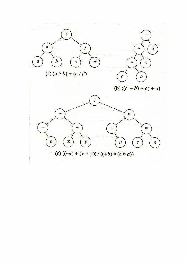
Binary trees are drawn similar to trees, with root node at the top. An

example for a binary tree is expression tree. Expression trees are used in

generation of optimal computer code to evaluate an expression. The

following figures show sample expression trees.

1133..22.. TThhee TTrreeee DDaattaa ssttrruuccttuurree..

Binary Tree Properties

The drawing of every binary tree with n (n>0) elements has

exactly (n-1) edges. The number of levels in a binary tree is called its depth or height.

A binary tree of height h, h0, has atleast h and at most 2h-1

elements in it.

The height of a binary tree that contains n, n0, elements is at

most n and at least log2(n+1).

A binary tree with height h, and contains exactly 2h-1 elements is called a Full Binary Tree.

The nodes in full binary tree are numbered sequentially, starting at

1, from level 1 to level h, and from left to right in each level.

A binary tree with maximum posible number of nodes at each level, except possibly the last is called a complete binary tree.

In a binary tree the maximum possible number of nodes at level k

is 2(k-1).

For an element numbered k, in a complete binary tree, if k=1, then

it is the root element. if k>1, then its parent has been assigned the

number (int) (k/2). Its left child is numbered 2k (no left child if 2k >

n), and right child is numbered 2k+1 (no right child if 2k+1 > n ,

where n is maximum number of nodes).

Binary Search Tree (BST) A BST is a binary tree with the following properties:

1. Every element has a key (or value). All keys are distinct.

2. The keys (if any) in the left subtree of the root are smaller than the

key in the root.

3. The keys (if any) in the right subtree of the root are larger than the

key in the root.

4. The left and right subtrees of the root are also binary search trees.

An example of a binary tree is shown below. (A circle with dotted line

indicates missing node.)

An example of a binary search tree in which elements have distinct keys

is shown below.

Level 1 node

Level 2 nodes

Level 3 nodes

A

B C

D E F

A

B C

E D

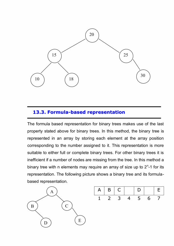
The formula based representation for binary trees makes use of the last

property stated above for binary trees. In this method, the binary tree is

represented in an array by storing each element at the array position

corresponding to the number assigned to it. This representation is more

suitable to either full or complete binary trees. For other binary trees it is

inefficient if a number of nodes are missing from the tree. In this method a

binary tree with n elements may require an array of size up to 2n-1 for its

representation. The following picture shows a binary tree and its formula-

based representation.

A B C D E

1 2 3 4 5 6 7

20

15 25

30 10 18

1133..33.. FFoorrmmuullaa--bbaasseedd rreepprreesseennttaattiioonn

The Linked representation is a popular way to store binary trees in

memory. This representation uses links or pointers. A node that has

exactly two link fields represents each element. The links are called left_child and right_child. In addition to these two link fields, each node

has a field has a field named data. An edge in the drawing of a binary tree

is represented by, a pointer from the parent node to the child node. This

pointer is placed in the appropriate link field of the parent node. Since an

n-element binary tree has exactly n-1 edges, (n+1) link fields are set to

zero or NULL. The following is the node class for linked representation of

binary trees:

template<class T>

class BinaryTreeNode{

public:

BinaryTreeNode() { left_child = right_child = 0; }

BinaryTreeNode(const T&e) {

data = e; left_child = right_child = 0;

}

private:

T data;

BinaryTreeNode<T> *left_child, // left subtree

*right_child; // right subtree.

};

1133..44.. LLiinnkkeedd rreepprreesseennttaattiioonn

Common binary tree operations: Some common

operations on binary trees are:

o Determine its height.

o Determine the number of elements in it.

o Make a copy.

o Delete the tree.

o Traverse and list the nodes in a tree.

o Search for a specific node in a tree.

The above said operations can be performed, by traversing the binary tree in a systematic manner. In a binary tree traversal, each element is

visited exactly once. During this visit the necessary action regarding this

node is taken. There are four common ways to traverse a binary tree.

They are:

A

B 0 C 0

D 0 0 E 0 0

Linked Representation of a binary tree

Preorder

Inorder

Postorder

Level order

The first three traversal methods are described in the following recursive

algorithms and procedures. Algorithm for preorder traversal:

step1: Visit the root node.

step2: Traverse the left subtree in preorder.

setp3: Traverse the right subtree in preorder.

Recursive implementation of the above algorithm:

template <class T>

void preorder(BinaryTreeNode<T> *t)

{ // preorder traversal of *t.

if( t) {

visit(t);

preorder(t->left_child); // start preorder traversal of left subtree.

preorder(t->right_child);//start preorder traversal of right subtree.

}

}

Algorithm for Inorder traversal:

step1: Traverse the left subtree in inorder.

step2: Visit the root node.

setp3: Traverse the right subtree in inorder.

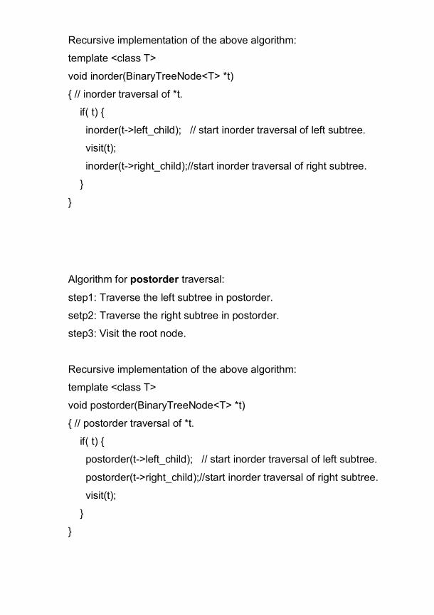
Recursive implementation of the above algorithm:

template <class T>

void inorder(BinaryTreeNode<T> *t)

{ // inorder traversal of *t.

if( t) {

inorder(t->left_child); // start inorder traversal of left subtree.

visit(t);

inorder(t->right_child);//start inorder traversal of right subtree.

}

}

Algorithm for postorder traversal:

step1: Traverse the left subtree in postorder.

setp2: Traverse the right subtree in postorder.

step3: Visit the root node.

Recursive implementation of the above algorithm:

template <class T>

void postorder(BinaryTreeNode<T> *t)

{ // postorder traversal of *t.

if( t) {

postorder(t->left_child); // start inorder traversal of left subtree.

postorder(t->right_child);//start inorder traversal of right subtree.

visit(t);

}

}

+

* /

d b c a

The visit() function in the above implementations defines the necessary

action to be taken on the nodes. Its simplest implementation is to display

the data at the node. In the preorder, inorder, and postorder traversal

methods the left subtree is traversed before the right subtree. The

difference in these traversals is in the time at which a node is visited. In

preorder each node is visited before its left and right subtree nodes are

visited. In inorder traversal, each node is visited after the left subtree

nodes and are visited and before the right subtree nodes. In postorder

traversal, each node is visited after both the left and right subtree nodes

are visited in that order. For the expression tree shown below the

preorder, inorder and postorder traversal methods give the prefix, infix

and postfix notations of the expression represented by the tree.

Preorder: +*ab/cd

Inorder: a*b+c/d

Postorder: ab*cd/+

The infix form of an expression is the form in which we normally write an

expression. In this form each binary operator appears between its

operands. In the prefix form each operator comes immediately before the

prefix from of its operands. The operands appear in left to right order. In

postfix notation each operator comes immediately after the postfix form of

its operands. The operands appear in left to right order.

Level order traversal: In a level order traversal of a binary tree, the

elements are visited by level from top to bottom. Within each level,

elements are visited from left to right. The following function shows an

implementation of the level order traversal of a binary tree.

// level order traversal.

template <class T>

void levelorder(BinaryTreeNode<T> *t)

{ // levelorder traversal of *t.

LinkedQueue<BinaryTreeNode<T>*> q;

while( t) {

visit(t);

if (t->left_child) q.add(t->left_child);

if (t->right_child) q.add(t->right_child);

// get next node to visit.

try { q.delete(t); } catch(OutOfBounds) {return;}

}

}

The space complexity of each of the four traversal programs is O(n) and

time complexity is (n), where n is the number of nodes in the binary tree.

Having some understanding of binary tree, we can specify an ADT for

binary tree as below.

AbstractDataType BinaryTree{

instances: collection elements; if not empty, the collection is

partitioned into a root, left subtree, and right subtree; each subtree is

also binary tree. operations: Create(): Create an empty binary tree. IsEmpty(): Return true if empty, false otherwise.

MakeTree(root, left, right): create a binary tree with root as the root

element, left and right subtrees.

PreOrder(): Do preorder traversal of the binary tree.

Inorder(): Do inorder traversal of the binary tree.

Postorder(): Do postorder traversal of the binary tree.

LevelOrder(): Do level order traversal of the binary tree.

}

1133..55.. BBiinnaarryy TTrreeee AADDTT && IImmpplleemmeennttaattiioonn

The following program gives the implementation of the binary tree ADT.

#ifndef BinaryTree_

#define BinaryTree_

int _count;

#include<iostream.h>

#include "lqueue.h"

#include "btnode2.h"

#include "xcept.h"

template<class E, class K> class BSTree;

template<class E, class K> class DBSTree;

template<class T>

class BinaryTree {

friend BSTree<T,int>;

friend DBSTree<T,int>;

public:

BinaryTree() {root = 0;};

~BinaryTree(){};

bool IsEmpty() const

{return ((root) ? false : true);}

bool Root(T& x) const;

void MakeTree(const T& element,

BinaryTree<T>& left, BinaryTree<T>& right);

void BreakTree(T& element, BinaryTree<T>& left,

BinaryTree<T>& right);

void PreOrder(void(*Visit)(BinaryTreeNode<T> *u))

{PreOrder(Visit, root);}

void InOrder(void(*Visit)(BinaryTreeNode<T> *u))

{InOrder(Visit, root);}

void PostOrder(void(*Visit)(BinaryTreeNode<T> *u))

{PostOrder(Visit, root);}

void LevelOrder(void(*Visit)(BinaryTreeNode<T> *u));

void PreOutput() {PreOrder(Output, root); cout << endl;}

void InOutput() {InOrder(Output, root);

cout << endl;}

void PostOutput() {PostOrder(Output, root);

cout << endl;}

void LevelOutput() {LevelOrder(Output);

cout << endl;}

void Delete() {PostOrder(Free, root); root = 0;}

int Height() const {return Height(root);}

int Size()

{_count = 0; PreOrder(Add1, root); return _count;}

private:

BinaryTreeNode<T> *root; // pointer to root

void PreOrder(void(*Visit)

(BinaryTreeNode<T> *u), BinaryTreeNode<T> *t);

void InOrder(void(*Visit)

(BinaryTreeNode<T> *u), BinaryTreeNode<T> *t);

void PostOrder(void(*Visit)

(BinaryTreeNode<T> *u), BinaryTreeNode<T> *t);

static void Free(BinaryTreeNode<T> *t) {delete t;}

static void Output(BinaryTreeNode<T> *t)

{cout << t->data << ' ';}

static void Add1(BinaryTreeNode<T> *t) {_count++;}

int Height(BinaryTreeNode<T> *t) const;

};

template<class T>

bool BinaryTree<T>::Root(T& x) const

{// Return root data in x.

// Return false if no root.

if (root) {x = root->data;

return true;}

else return false; // no root

}

template<class T>

void BinaryTree<T>::MakeTree(const T& element,

BinaryTree<T>& left, BinaryTree<T>& right)

{// Combine left, right, and element to make new tree.

// left, right, and this must be different trees.

// create combined tree

root = new BinaryTreeNode<T>

(element, left.root, right.root);

// deny access from trees left and right

left.root = right.root = 0;

}

template<class T>

void BinaryTree<T>::BreakTree(T& element,

BinaryTree<T>& left, BinaryTree<T>& right)

{// left, right, and this must be different trees.

// check if empty

if (!root) throw BadInput(); // tree empty

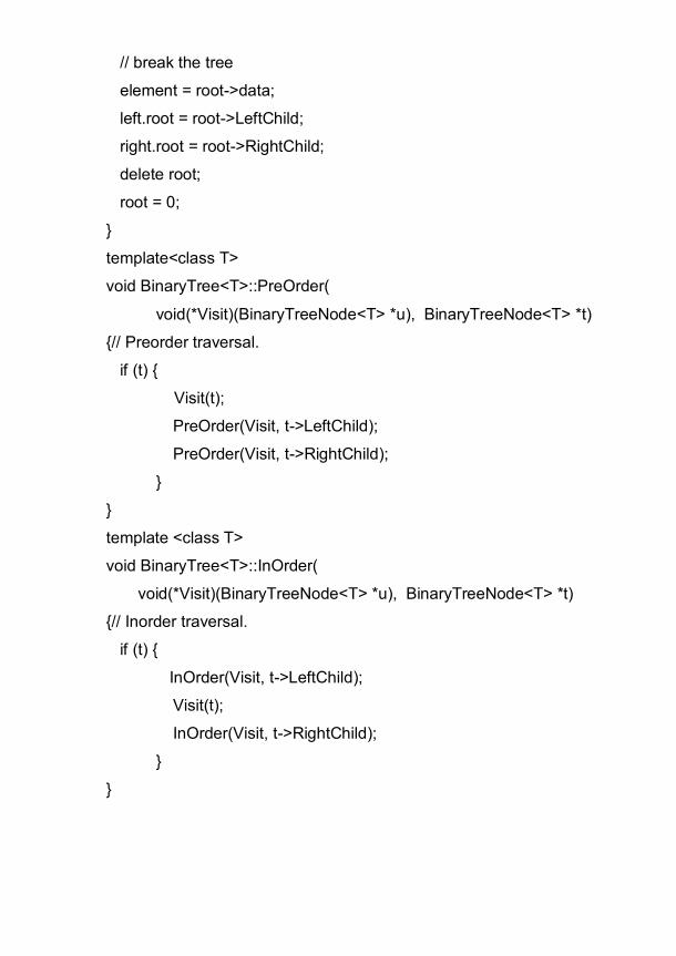
// break the tree

element = root->data;

left.root = root->LeftChild;

right.root = root->RightChild;

delete root;

root = 0;

}

template<class T>

void BinaryTree<T>::PreOrder(

void(*Visit)(BinaryTreeNode<T> *u), BinaryTreeNode<T> *t)

{// Preorder traversal.

if (t) {

Visit(t);

PreOrder(Visit, t->LeftChild);

PreOrder(Visit, t->RightChild);

}

}

template <class T>

void BinaryTree<T>::InOrder(

void(*Visit)(BinaryTreeNode<T> *u), BinaryTreeNode<T> *t)

{// Inorder traversal.

if (t) {

InOrder(Visit, t->LeftChild);

Visit(t);

InOrder(Visit, t->RightChild);

}

}

template <class T>

void BinaryTree<T>::PostOrder( void(*Visit)(BinaryTreeNode<T> *u),

BinaryTreeNode<T> *t) {// Postorder traversal.

if (t) {

PostOrder(Visit, t->LeftChild);

PostOrder(Visit, t->RightChild);

Visit(t);

}

}

template <class T>

void BinaryTree<T>::LevelOrder( void(*Visit)(BinaryTreeNode<T> *u))

{// Level-order traversal.

LinkedQueue<BinaryTreeNode<T>*> Q;

BinaryTreeNode<T> *t;

t = root;

while (t) {

Visit(t);

if (t->LeftChild) Q.Add(t->LeftChild);

if (t->RightChild) Q.Add(t->RightChild);

try {Q.Delete(t);

}

catch (OutOfBounds) {return;}

}

}

template <class T>

int BinaryTree<T>::Height(BinaryTreeNode<T> *t) const

{// Return height of tree *t.

if (!t) return 0; // empty tree

int hl = Height(t->LeftChild); // height of left

int hr = Height(t->RightChild); // height of right

if (hl > hr) return ++hl;

else return ++hr;

}

#endif

A graph is a collection of nodes, pairs of which are joined by lines or edges. A more formal definition can be given as: Definition: A graph G = (V,E) is an ordered pair of finite sets V and E. The elements of V are called vertices or nodes or points. The elements of E are called edges. Each edge in E joins two different vertices of V and is denoted by the ordered pair (i,j), where I and j are the two vertices. A graph is displayed with nodes as circles and edges as lines. The edges may have a orientation. An edge with an orientation is called a directed edge. An undirected edge has no orientation. If all the edges in a graph are directed then it is called a directed graph or digraph. Two vertices i and j are called adjacent if and only if there is an edge from vertex i to vertex j. The edge (i,j) is incident on vertices i and j. When weights have been assigned to edges, then that graph is called a weighted graph. Some examples of graphs are shown below:

1133..66.. GGrraapphh DDaattaa SSttrruuccttuurree

digraph

1

3 2

4

5

6 1

3 2

4

graph

Path: a sequence of vertices P = i1, i2,… ,ik is an i1 to ik path in the graph or digraph G = (V,E) if and only if the edge (ij,ij+1) is in E for every j, 1 j < k. Simple path: It is a path in which all vertices, except possibly the first and last, are different. Length of a path: The length of a path is the number of edges involved in that path. Cycle: A cycle is a simple path with the same start and end vertex. Subgraph: A graph H is a subgraph of another graph G if and only if its vertex and edge sets are subsets of those of G.

weighted graph

12

10

18 24

1

3 6 7

2

5

4

28

16 14

25

22

Connected graph: A graph G is connected if and only if there is a path between every pair of vertices in G. Note: A connected undirected graph that contains no cycles is a tree. Spanning tree: A subgraph of G that contains all the vertices of G and is a tree is a spanning tree of G. Some properties of graphs:

1) A connected graph with n vertices must have at least n-1 edges. 2) Let G be an undirected graph. The degree di of vertex i is the

number of edges incident on vertex i. 3) An n-vertex graph with n(n-1)/2 edges is a complete graph. 4) Let G be a digraph. The in-degree di

in of vertex i is the number of edges incident to i. The out-degree di

out of vertex i is the number of edges incident from this vertex.

5) A complete digraph with n vertices contains exactly n(n-1) directed edges.

The ADTs Graph and Digraph The abstract data type Graph refers to undirected graphs. The abstract data type Digraph refers to digraphs. The below listing gives the ADTs Graph and Digraph. AbstractDataType Graph{

instances a set V of vertices and a set E of edges

operations Create(n): create an undirected graph with n vertices and no edges Exist(i,j): return true if edge (i,j) exists, false otherwise Edges(): return the number of edges in the graph Vertices(): return the number of vertices in the graph Add(i,j): add the edge (i,j) Delete(i,j): delete the edge (i,j) Degree(i): return the degree of vertex i.

}

AbstractDataType DiGraph{ instances

a set V of vertices and a set E of edges operations

Create(n): create a directed graph with n vertices and no edges Exist(i,j): return true if edge (i,j) exists, false otherwise Edges(): return the number of edges in the graph Vertices(): return the number of vertices in the graph Add(i,j): add the edge (i,j) to the graph Delete(i,j): delete the edge (i,j) InDegree(i): return the in-degree of vertex i. OutDegree(i): return the out-degree of vertex i

} The most frequently used representation schemes for graphs and digraphs are adjacency based: adjacency matrices, and adjacency lists. Adjacency Matrix The adjacency matrix of an n-vertex graph G = (V,E) is an n x n matrix A. Each element of A is either zero or one. We shall assume that V = {1,2,…,n}. If G is an undirected graph, then the elements of A are defined as follows:

1 if (i,j) E or (j,i) E A(i,j) =

0 otherwise If G is a digraph, then the elements of A are defined as follows:

1 if (i,j) E A(i,j) =

0 otherwise

1133..77.. AAddjjaacceennccyy MMaattrriixx aanndd AAddjjaacceennccyy LLiissttss..

The adjacency matrices for two graphs are as shown here.

Adjacency matrix:

1 2 3 4 1 0 1 1 1 2 1 0 1 0 3 1 1 0 1 4 1 0 1 0

Adjacency matrix:

1 2 3 4 5 6 1 0 0 1 1 0 0 2 0 0 1 0 0 0 3 0 0 0 0 1 1 4 0 1 1 0 0 0 5 1 0 1 1 0 0 6 0 0 0 0 1 0

The n x n adjacency matrix A may be mapped into a array of the same size or of size (n+1) x (n+1) of type int using the mapping A(i,j) = A[i][j], where 1 i n, and 1 j n. Adjaceny Lists In the case of adjaceny lists (or linked-adjacency lists), each adjacency list is maintained as a chain. The adjacency lists of the above given two grapsh are as shown.

1

3 2

4

1

3 2

4

5

6

Adjacency List:

Adjacency List:

1

3 2

4

h

[1]

[2]

[3]

[4]

4

2 3 0

3 1 0

1

2 4 1 0

3 0

1

3 2

4

5

6 3 4 0

3 0

2

5 6 0

3 0

[1]

[2]

[3]

[4]

[5]

[6]

1 3 4 0

5 0

h

Many operations on graph require traversing its nodes. There are two standard ways to do this. These are known as search methods. They are Breadth-First search and Depth-First Search. Although both methods are popular, Depth-First search is used frequently. Breadth-First Search (BFS) This method proceeds by starting at a vertex and identifying all vertices reachable from it. i.e. identifying all adjacent vertices to it and repeating this procedure from each such vertex in that order until all the vertices are visited. The queue data structure is used to perform this search. The tree resulting from this search is called Breadth first search spanning tree. The following is the pseudo code for BFS. //Breadth first search beginning at vertex v. Label vertex v as reached; Initialize Q to be a queue with only v in it; while(Q is not empty) {

Delete a vertex w from the queue; Let u be a vertex (if any) adjacent from w;

while(u){ if (u has not been labeled) { Add u to the queue; Label u as reached; u = next vertex that is adjacent from w; } }

}

1133..88.. BBrreeaaddtthh--FFiirrsstt aanndd DDeepptthh--FFiirrsstt SSeeaarrcchh

Depth-First Search (DFS) This is an alternative to BFS. Starting at a vertex v, the DFS proceeds as follows: First the vertex v s marked as visited, and then an unreached vertex u adjacent from v is selected. If such a vertex does not exist, the search terminates. If u exists, the DFS is now initiated from u. When this search is completed, another vertex adjacent from v is selected, and the process continues until no such un visited vertex exists. The tree obtained from DFS is called DFS spanning tree. The pseudo code for DFS is given below. //Depth first search beginning at vertex v. Label vertex v as reached; Initialize S to be a stack with only v on its top; while(S is not empty) {

pop a vertex w from the stack S; Let u be a vertex (if any) adjacent from w;

if (u has not been labeled) { push u on to the stack S; Label u as reached; } }

}

(a) Directed Graph (b)Breadth-First Search Tree of Graph in (a).

In computer science, a tree is a widely-used computer data structure that emulates a tree structure with a set of linked nodes. It is a special case of a graph. A tree is considered as a recursive structure that usually maps an ordered set of data from an internal definition to some data space. Each node in a tree has zero or more child nodes, which are below it in the tree. A node that has a child is called the child's parent node. A child has at most one parent; The topmost node in a tree is called the root node. Being the topmost node, the root node will not have parents. Nodes at the bottom most level of the tree are called leaf nodes. Since they are at the bottom most level, they will not have any children. A binary tree is a rooted tree in which every node has at most two children. A full binary tree is a tree in which every node has zero or two children. Also known as a proper binary tree. A perfect binary tree is a full binary tree in which all leaves (vertices with zero children) are at the same depth (distance from the root, also called height). Pre-order, in-order, and post-order traversal visit each node in a tree by recursively visiting each node in the left and right subtrees of the root. If the root node is visited before its subtrees, this is preorder; if after, postorder; if between, in-order. In-order traversal is useful in binary search trees, where this traversal visits the nodes in increasing order. a graph is an abstract data type (ADT) that consists of a set of nodes and a set of edges that establish relationships (connections) between the nodes. A graph G is defined as follows: G=(V,E), where V is a finite, non-empty set of vertices and E is a set of edges (links between pairs of vertices). When the edges in a graph have no direction, the graph is called undirected, otherwise called directed. In practice, some information is associated with each node and edge. An adjacency list associates each node with an array of incident edges. If no information is required to be stored in edges, only in nodes, these arrays can simply be pointers to other nodes and thus represent edges with little memory requirement. An advantage of this approach is that new nodes can be added to the graph easily, and they can be connected with existing nodes simply by adding elements to the appropriate arrays. A disadvantage is that determining whether an edge exists between two nodes requires O(n) time, where n is the average number of incident edges per node.

1133..99.. SSuummmmaarryy

An alternative way is to keep a square matrix (a two-dimensional array) M of boolean values (or integer values, if the edges also have weights or costs associated with them). The entry Mi,j then specifies whether an edge exists that goes from node i to node j. An advantage of this approach is that finding out whether an edge exists between two nodes becomes a trivial constant-time memory look-up. Similarly, adding or removing an edge is a constant-time memory access. In depth-first order, we always attempt to visit the node farthest from the root that we can, but with the caveat that it must be a child of a node we have already visited. Unlike a depth-first search on graphs, there is no need to remember all the nodes we have visited, because a tree cannot contain cycles. Preorder, in-order, and postorder traversal are all special cases of this. Contrasting with depth-first order is breadth-first order, which always attempts to visit the node closest to the root that it has not already visited.

Tree A tree is a non-linear data structure in which elements are

represented as nodes and are linked together in hierarchical fashion. Root

A root node is a specially chosen node in a tree data structure at which all operations on the tree begin Degree

The number of children of a node is called the degree of that node. Leaf

A node with no child nodes is called leaf. Binary Tree

A binary tree is a rooted tree in which every node has at most two children. Graph

A graph is a collection of nodes, pairs of which are joined by lines or edges.

1133..1100.. TTeecchhnniiccaall TTeerrmmss

1. Define a Tree. Describe its properties. 2. Describe Tree Traversal techniques. 3. Implement a Binary Tree and its operations using C++. 4. Discuss different Memory Representations of Trees. 5. Define a Graph. Discuss its Memory Representations. 6. State the difference and similarity between a Tree and a Graph. 7. Discuss DFS and BFS procedures. 8. Implement Graph search algorithms using C++; 9. Write the ADTs for Tree and Graph.

1133..1111.. MMooddeell QQuueessttiioonnss

1133..1122.. RReeffeerreenncceess