Les tests bases sur les permutationsEchantillons de tailles faibles et nombre important de variables

Yohann.Foucher@univ-nantes.fr

Equipe d’Accueil 4275 ”Biostatistique, recherche clinique et mesures subjectives ensante”, Universite de Nantes

MASTER 1 Bionformatique et Biostatistique - UE donnees omics

1 / 1

Plan

2 / 1

Plan

3 / 1

Problematique

� Les nouveaux outils d’analyse a haut debit permettent la mesuresimultanee de milliers caracteristiques d’un individu

ex : Puces ADN : elles peuvent mesurer plusieurs milliers de genes.

� Objectif : identifier des caracteristiques differemment exprimeesentre plusieurs groupes.

ex : identifier les genes differemment exprimes entre les malades etles non-malades.

4 / 1

Problematique

Update on Gene Expression Analysis, Proteomics, and Network Discovery

Gene Expression Analysis, Proteomics, andNetwork Discovery1

Sacha Baginsky, Lars Hennig, Philip Zimmermann, and Wilhelm Gruissem*

Department of Biology and Zurich-Basel Plant Science Center, ETH Zurich Universitatstrasse 2,8129 Zurich, Switzerland

Technological advances in biological experimenta-tion are now enabling researchers to investigate livingsystems on an unprecedented scale by studying ge-nomes, proteomes, or molecular networks in theirentirety. Genomics technologies have led to a para-digm shift in biological experimentation because theymeasure (profile) most or even all components of oneclass (e.g. transcripts, proteins, etc.) in a highly parallelway. Whether gene expression analysis using micro-arrays, proteome and metabolome analysis usingmass spectrometry, or large-scale screens for geneticinteractions, high-throughput profiling technologiesprovide a rich source of quantitative biologicalinformation that allows researchers to move beyonda reductionist approach by both integrating and un-derstanding interactions between multiple compo-nents in cells and organisms (Fig. 1; for a recentupdate of bioinformatics tools, see Pitzschke andHirt, 2010). Currently, most genomics experimentsinvolve profiling transcripts, proteins, or metabolites.Increasing efforts to complement molecular data withphenotypic information will further advance our un-derstanding of the quantitative relationships betweenmolecules in directing systems behavior and function.In the following Update we will briefly review recentadvances in the field and highlight advantages andlimitations of current approaches to develop models ofgenetic and molecular networks that aim to describeemergent properties of plant systems.

GENOMICS TECHNOLOGIES: THE POWER OFGENOME-SCALE QUANTITATIVE DATARESOLUTION PROFILING TRANSCRIPTOMES

Transcript profiling offers the largest coverage and awide dynamic range of gene expression informationand can often be performed genome wide. Micro-

arrays are currently most popular for transcriptprofiling and can be readily afforded by manylaboratories. Various commercial and academic micro-array platforms exist that vary in genome coverage,availability, specificity, and sensitivity (Table I). Micro-arrays manufactured by Affymetrix are probably mostcommonly used in plant biology (Redman et al., 2004;Rehrauer et al., 2010), but commercial arrays fromAgilent or arrays from the academic Complete Arabi-dopsis Transcriptome MicroArray (CATMA) consor-tium are often used as well (for review, see Busch andLohmann, 2007). Serial analysis of gene expression(SAGE) and massively parallel signature sequencing(MPSS) are well-established alternatives to microar-rays. Both techniques can be superior to microarraysbecause they do not depend on prior probe selection.More recently, direct sequencing of transcripts byhigh-throughput sequencing technologies (RNA-Seq)has become an additional alternative to microarraysand is superseding SAGE and MPSS (Busch andLohmann, 2007). Like SAGE and MPPS, RNA-Seqdoes not depend on genome annotation for priorprobe selection and avoids biases introduced dur-ing hybridization of microarrays. On the other hand,RNA-Seq poses novel algorithmic and logistic chal-lenges, and current wet-lab RNA-Seq strategies re-quire lengthy library preparation procedures.Therefore, RNA-Seq is the method of choice in projectsusing nonmodel organisms and for transcript discov-ery and genome annotation. Because of their robustsample processing and analysis pipelines, often micro-arrays are still a preferable choice for projects thatinvolve large numbers of samples for profiling tran-scripts in model organisms with well-annotated ge-nomes. Tools such as Genevestigator (Hruz et al., 2008)and MapMan (Usadel et al., 2009) allow researchers toorganize large gene expression datasets and analyzethem for relational networks within a single experi-ment or across many experiments (contextual meta-analysis).

PROFILING EPIGENOMES AND TRANSCRIPTIONFACTOR BINDING

Much control of gene expression occurs at the levelof transcription, and information on genome-widechromatin profiles (epigenomes) and transcriptionfactor binding to promoters is needed to decipher

1 This work was supported by the European Union (EUFramework Program 6, AGRON-OMICS; grant no. LSHG–CT–2006–037704), the Swiss National Science Foundation, CTI (SwissInnovation Promotion Agency), ETH Zurich, and the FunctionalGenomics Center Zurich for our profiling experiments.

* Corresponding author; e-mail wgruissem@ethz.ch.The author responsible for distribution of materials integral to the

findings presented in this article in accordance with the policydescribed in the Instructions for Authors (www.plantphysiol.org) is:Wilhelm Gruissem (wgruissem@ethz.ch).

www.plantphysiol.org/cgi/doi/10.1104/pp.109.150433

402 Plant Physiology�, February 2010, Vol. 152, pp. 402–410, www.plantphysiol.org � 2009 American Society of Plant Biologists

Update on Gene Expression Analysis, Proteomics, and Network Discovery

Gene Expression Analysis, Proteomics, andNetwork Discovery1

Sacha Baginsky, Lars Hennig, Philip Zimmermann, and Wilhelm Gruissem*

Department of Biology and Zurich-Basel Plant Science Center, ETH Zurich Universitatstrasse 2,8129 Zurich, Switzerland

Technological advances in biological experimenta-tion are now enabling researchers to investigate livingsystems on an unprecedented scale by studying ge-nomes, proteomes, or molecular networks in theirentirety. Genomics technologies have led to a para-digm shift in biological experimentation because theymeasure (profile) most or even all components of oneclass (e.g. transcripts, proteins, etc.) in a highly parallelway. Whether gene expression analysis using micro-arrays, proteome and metabolome analysis usingmass spectrometry, or large-scale screens for geneticinteractions, high-throughput profiling technologiesprovide a rich source of quantitative biologicalinformation that allows researchers to move beyonda reductionist approach by both integrating and un-derstanding interactions between multiple compo-nents in cells and organisms (Fig. 1; for a recentupdate of bioinformatics tools, see Pitzschke andHirt, 2010). Currently, most genomics experimentsinvolve profiling transcripts, proteins, or metabolites.Increasing efforts to complement molecular data withphenotypic information will further advance our un-derstanding of the quantitative relationships betweenmolecules in directing systems behavior and function.In the following Update we will briefly review recentadvances in the field and highlight advantages andlimitations of current approaches to develop models ofgenetic and molecular networks that aim to describeemergent properties of plant systems.

GENOMICS TECHNOLOGIES: THE POWER OFGENOME-SCALE QUANTITATIVE DATARESOLUTION PROFILING TRANSCRIPTOMES

Transcript profiling offers the largest coverage and awide dynamic range of gene expression informationand can often be performed genome wide. Micro-

arrays are currently most popular for transcriptprofiling and can be readily afforded by manylaboratories. Various commercial and academic micro-array platforms exist that vary in genome coverage,availability, specificity, and sensitivity (Table I). Micro-arrays manufactured by Affymetrix are probably mostcommonly used in plant biology (Redman et al., 2004;Rehrauer et al., 2010), but commercial arrays fromAgilent or arrays from the academic Complete Arabi-dopsis Transcriptome MicroArray (CATMA) consor-tium are often used as well (for review, see Busch andLohmann, 2007). Serial analysis of gene expression(SAGE) and massively parallel signature sequencing(MPSS) are well-established alternatives to microar-rays. Both techniques can be superior to microarraysbecause they do not depend on prior probe selection.More recently, direct sequencing of transcripts byhigh-throughput sequencing technologies (RNA-Seq)has become an additional alternative to microarraysand is superseding SAGE and MPSS (Busch andLohmann, 2007). Like SAGE and MPPS, RNA-Seqdoes not depend on genome annotation for priorprobe selection and avoids biases introduced dur-ing hybridization of microarrays. On the other hand,RNA-Seq poses novel algorithmic and logistic chal-lenges, and current wet-lab RNA-Seq strategies re-quire lengthy library preparation procedures.Therefore, RNA-Seq is the method of choice in projectsusing nonmodel organisms and for transcript discov-ery and genome annotation. Because of their robustsample processing and analysis pipelines, often micro-arrays are still a preferable choice for projects thatinvolve large numbers of samples for profiling tran-scripts in model organisms with well-annotated ge-nomes. Tools such as Genevestigator (Hruz et al., 2008)and MapMan (Usadel et al., 2009) allow researchers toorganize large gene expression datasets and analyzethem for relational networks within a single experi-ment or across many experiments (contextual meta-analysis).

PROFILING EPIGENOMES AND TRANSCRIPTIONFACTOR BINDING

Much control of gene expression occurs at the levelof transcription, and information on genome-widechromatin profiles (epigenomes) and transcriptionfactor binding to promoters is needed to decipher

1 This work was supported by the European Union (EUFramework Program 6, AGRON-OMICS; grant no. LSHG–CT–2006–037704), the Swiss National Science Foundation, CTI (SwissInnovation Promotion Agency), ETH Zurich, and the FunctionalGenomics Center Zurich for our profiling experiments.

* Corresponding author; e-mail wgruissem@ethz.ch.The author responsible for distribution of materials integral to the

findings presented in this article in accordance with the policydescribed in the Instructions for Authors (www.plantphysiol.org) is:Wilhelm Gruissem (wgruissem@ethz.ch).

www.plantphysiol.org/cgi/doi/10.1104/pp.109.150433

402 Plant Physiology�, February 2010, Vol. 152, pp. 402–410, www.plantphysiol.org � 2009 American Society of Plant Biologists

5 / 1

Problematique

most suitable PTPs for the detection and quantificationof specific proteins. However, only experimental dataprovide the necessary reliability for PTP selectionbecause in practice PTP prediction often deviatesfrom experimental observations. Therefore, effortsare under way to catalogue PTPs for model organismproteomes. Proteome maps for Arabidopsis generatedPTPs for 4,105 proteins, many of which may be opti-mal for the detection of proteins in different organs(Baerenfaller et al., 2008).Similar quantitative approaches are also used for

metabolites, because in addition to RNA and proteinlevels, understanding the function and behavior ofmetabolic networks requires global information aboutmetabolite concentrations and fluxes as well. In recentyears, much progress has been made in metabolicprofiling, and the interested reader is referred to recentreviews (e.g. Issaq et al., 2009, and refs. therein).

TRANSCRIPTS AND MORE TRANSCRIPTS:WHAT CAN WE LEARN FROM GENEEXPRESSION ANALYSIS?

During the analysis of large gene expression data-sets the researcher is often confronted with severalquestions. How do we interpret a mathematical rela-tionship between genes or between genes and condi-tions? For example, does a high correlation betweentwo genes mean that they are coregulated, or couldone of them be the positive regulator of the other? Orcan we assume that they are involved in the same

pathway or biological process? Although it is notpossible to answer these questions conclusively fromgene expression data alone, a number of parallelapproaches can be useful to distinguish between dif-ferent scenarios. For example, Gene Ontology enrich-ment analysis can provide confidence that a givengene cluster is enriched in genes that are known tohave a common function, cellular location, or biolog-ical process. Similarly, conserved cis-regulatory ele-ments in the promoters of genes from the same clusterindicate that they are likely coregulated. Althoughthese methods do not establish proof of the nature ofthe relationship between genes, they allow formulat-ing hypotheses that can be tested in the laboratory. Insummary, although gene expression analysis by itselfis rather descriptive (i.e. describing how genes re-spond to various test conditions or tissues), it is avaluable validation tool and an excellent starting pointto study novel cellular process and to formulate novelhypotheses.

A major challenge of genome-scale transcriptionanalysis is the very large number of predictors (genes)compared to a generally small number of measure-ments (microarrays). Without appropriate statisticalmeasures to correct for multiple testing and includingfalse discovery rates, almost any approach will yieldsignificant genes, including many false positives. Thecreation of large databases in recent years has broughtan additional layer of complexity and precautions totake (see Table II). For example, large databases suchas Genevestigator (Hruz et al., 2008) not only profile alarge number of genes, but also allow contextual meta-

Table II. Overview of some of the most popular plant gene expression microarray platforms and the number of available experimentsin ArrayExpress

The Arabidopsis ATH1 array is the most frequently used microarray, followed by the CATMA 25k and 23k arrays. In all, approximately 750Arabidopsis microarray experiments have been published so far. Rice (Oryza sativa) and barley (Hordeum vulgare) are the second and third plantspecies in terms of microarray experiments published. Soybean (Glycine max) also has a high number of arrays, but this is due to a single very largeexperiment containing 2,521 arrays. IPK, Leibniz Institute of Plant Genetics and Crop Plant Research; TIGR, The Institute for Genomic Research.

Species ProviderArray

FormatArray Name Experiments Arrays

Arabidopsis Affymetrix 8K AG 41 352Affymetrix 22K ATH1 554 8,895Agilent 22K Arabidopsis 2 34 253Agilent 44K Arabidopsis 3 7 60CATMA 25K CATMA2_URGV to CATMA2.3_URGV 83 851CATMA 23K CATMA Arabidopsis 23K array 50 1,290TIGR 26K TIGR Arabidopsis whole genome 6 264

Rice Affymetrix 57K GeneChip Rice Genome Array 29 418Agilent 21K Agilent Rice Oligo Microarray 22 164

Barley Affymetrix 22K GeneChip Barley Genome Array 35 1,165IPK 6K + 4K IPK barley PGRC1_A and B 7 324

Medicago Affymetrix 61K GeneChip Medicago Genome Array 19 218Maize Affymetrix 17K GeneChip Maize Genome Array 22 370Soybean Affymetrix 61K GeneChip Soybean Genome Array 22 3,236Tomato (Solanum

lycopersicum)Affymetrix 10K GeneChip Tomato Genome Array 6 127

Grape (Vitis vinifera) Affymetrix 16K GeneChip Vitis vinifera Genome Array 6 239Wheat (Triticum aestivum) Affymetrix 61K GeneChip Wheat Genome Array 25 811Total 968 19,037

Gene Expression Analysis, Proteomics, and Network Discovery

Plant Physiol. Vol. 152, 2010 405

6 / 1

Limites des methodes traditionnelles

� Methode : calcul des probabilites critiques (pvalue ∗).

→ Soit pj la probabilite critique associee au gene j .

� Supposons k = 1000 genes etudies.

� Deux groupes A et B de tailles NA et NB

� On observe les expressions du gene j :

� xjA1, xjA2, ..., xjANA dans le groupe A→ moyenne : xjA et ecart-type sjA

� xjB1, xjB2, ..., xjBNB dans le groupe B→ moyenne : xjB et ecart-type sjB

∗. probabilite que la difference observee soit due au hasard (probabilitecritique en francais) 7 / 1

Limites des methodes traditionnelles

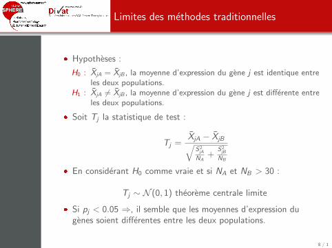
� Hypotheses :

H0 : XjA = XjB , la moyenne d’expression du gene j est identique entreles deux populations.

H1 : XjA 6= XjB , la moyenne d’expression du gene j est differente entreles deux populations.

� Soit Tj la statistique de test :

Tj =XjA − XjB√

S2jA

NA+

S2jB

NB

� En considerant H0 comme vraie et si NA et NB > 30 :

Tj ∼ N (0, 1) theoreme centrale limite

� Si pj < 0.05 ⇒, il semble que les moyennes d’expression dugenes soient differentes entre les deux populations.

8 / 1

Limites des methodes traditionnelles

> N.A <- 100> N.B <- 100> k <- 1000> E.A <- rnorm(N.A, mean=0, sd=1)> E.B <- rnorm(N.B, mean=0, sd=1)> E.A

[1] 0.259767012 0.104756575 0.309616563 0.624475170 -0.627431940[6] 1.262903438 0.835544333 -0.806822577 0.636655175 0.001920257[11] 1.308219156 -0.593271319 -1.781291756 0.928474836 0.047191736[16] 0.097193687 0.188600260 -0.896055910 -0.780684894 -0.903431156[21] -1.404657666 -1.112908505 -0.482515098 -0.305200701 -2.959189767[26] -0.619398436 0.964401705 -0.677996115 0.570158887 0.500985102[31] 1.310491882 -0.026689214 -0.834014767 1.487892811 -0.806169717[36] 0.875037438 -0.615388338 -0.767584042 -1.006066605 -1.790111173[41] -0.711082650 2.402996565 1.579152671 -1.360627507 0.557139166[46] -0.233817692 0.906085507 -0.816444847 -0.745482092 -1.768722704[51] 0.653054726 -1.139583695 -0.799815577 -1.194266380 -0.224372307[56] -0.892277328 -0.986516414 1.168128361 -1.765169418 -0.127545667[61] 2.073436445 -0.679708254 -1.397863208 -1.922954639 -0.310621692[66] 0.691923479 0.378232604 0.304669060 -1.386852628 -0.352114839[71] -1.356227305 0.265875723 -1.064897180 0.506978879 0.241024861[76] -0.959748501 0.678611734 -0.068313695 0.593750095 -0.370472628[81] 0.454820690 0.342254341 -0.746135230 -0.955464046 1.456725980[86] 0.388536819 -0.162063823 0.708618518 0.358394361 -0.336222683[91] 0.580267446 0.008241462 0.808807889 0.680924584 -0.872851582[96] 0.024976298 -2.223802297 -0.706544494 -1.916743943 2.188871939

> E.B

[1] 2.274006261 -0.177904256 -0.517614196 1.867644610 -0.889814720[6] -0.345420349 -0.056324463 1.640423490 -1.071025365 -0.726124355[11] 0.007195359 -0.115107492 1.813858939 0.731196085 -0.888783731[16] 1.023850478 0.056208381 1.109414726 -0.354122506 -0.801464288[21] -0.344592521 -1.094493819 2.464724754 -0.224061827 0.490715189[26] 0.773812657 -0.913603509 0.173088042 -0.033537909 -0.802618082[31] 0.072162132 0.290617942 0.008683900 1.425903421 2.066885394[36] 0.356077263 -0.380686772 0.622003033 -0.995290475 -1.461427800[41] 0.485610146 -0.141726073 -0.524877686 0.921722197 -0.582693895[46] -1.652037170 1.045227827 -0.107041561 -0.134118706 1.786325022[51] 1.960097265 1.402754711 -0.663989734 -1.605792976 -0.345822479[56] 0.625123386 -0.120433782 1.508371309 -2.464148126 0.564656250[61] 0.778728700 2.105730304 -2.402203109 0.594559532 0.375680395[66] 0.831399081 -0.378015702 0.347715392 -1.183469810 -0.418527631[71] 1.104859638 -0.390936467 0.878613248 -0.045749960 -0.542231378[76] 0.566612958 -1.989790346 1.998894492 1.760628557 -0.368664506[81] 0.767826257 -0.130066314 -2.528992623 1.657669258 -0.246187302[86] -0.602133683 -0.786925388 1.371395046 0.690559781 -0.557043214[91] 0.264796796 -0.826886138 -0.100128426 -0.040564443 -0.879317927[96] -0.235905015 0.525496584 1.363851421 -0.891425991 -0.939637293

9 / 1

Limites des methodes traditionnelles

> t.test(E.A, E.B)

Welch Two Sample t-test

data: E.A and E.Bt = -1.868, df = 197.301, p-value = 0.06324alternative hypothesis: true difference in means is not equal to 095 percent confidence interval:-0.56670225 0.01535635sample estimates:mean of x mean of y-0.1703542 0.1053187

> t.test(E.A, E.B)$p.value

[1] 0.06324423

10 / 1

Limites des methodes traditionnelles

> pvalues <- rep(NA, k)> for(j in 1:k)+ {+ E.A <- rnorm(N.A, mean=0, sd=1)+ E.B <- rnorm(N.B, mean=0, sd=1)+ pvalues[j] <- t.test(E.A, E.B)$p.value+ }> pvalues[1:10]

[1] 0.8066186 0.8363131 0.8869664 0.4589966 0.3805023 0.2423012[7] 0.2317830 0.5548061 0.9269442 0.1275307

> table(pvalues<0.05)

FALSE TRUE939 61

> table(pvalues<0.05)/k

FALSE TRUE0.939 0.061

> hist(pvalues, nclass=30, xlab="p-values", main="")> abline(v=0.05, col="red3", lwd=3, lty=2)

11 / 1

Limites des methodes traditionnelles

p−values

Fre

quen

cy

0.0 0.2 0.4 0.6 0.8 1.0

010

2030

4050

60

12 / 1

Problematique

Nombre variables >>> Nombre de sujets

1 Impossibilite de connaitre la distribution des statistiques de testsous l’hypothese nulle.

2 Comparaisons multiples et augmentation du nombre d’erreurs de1ere espece.

13 / 1

Plan

14 / 1

Multiple Test Procedure (MTP) : References

Article M.J. van der Laan, S. Dudoit, K.S. Pollard (2004),Augmentation Procedures for Control of the GeneralizedFamily-Wise Error Rate and Tail Probabilities for the Proportionof False Positives, Statistical Applications in Genetics andMolecular Biology, 3(1).

Livre S. Dudoit and M.J. van der Laan. Multiple Testing Proceduresand Applications to Genomics. Springer Series in Statistics.Springer, New York, 2008.

R Package ”multtest”.

15 / 1

MTP : Deux principes fondamentaux

1 Estimation non-parametrique des distributions des statistiquesde test sous H0.

2 Penalisation des probabilites critiques pour la prise en comptedes comparaisons multiples.

16 / 1

Plan

17 / 1

Principe de la permutation

� Permutation des libelles des colonnes (groupes A/B).

� Distributions des genes deviennent independantes des groupes.

Donnees observees : H0 ou H1 ?

Groupes A A A A A B B B B BValeurs 1.2 2.4 0.5 0.7 1.0 2.2 3.4 1.5 0.7 0.9

⇓

Donnees permutees : H0 est vraie

Groupes B A B B A B A B A AValeurs 1.2 2.4 0.5 0.7 1.0 2.2 3.4 1.5 0.7 0.9

18 / 1

Construction des distributions sous H0 et calculdes p-values

� On calcul classiquement la statistique de test pour les k genes :

t1, t2, ..., tk

� On realise B iterations. Pour chaque iteration (b = 1, 2, ...,B) :

� Permutation des colonnes.� Calcul des statistiques de test pour chaque gene :

t(b)1 , t

(b)2 , ..., t

(b)k

� Calcul des probabilites critiques (non corrigees) :

p∗j =

∑Bb=1 I (|t

(b)j | ≥ |tj |)B

ou I (a) est egale a 1 si la condition a est respectee et 0 sinon.

19 / 1

Exemple

> Groupes <- c("A", "A", "A", "A", "A", "B", "B", "B", "B", "B")> Valeurs <- c(1.2, 2.4, 0.5, 0.7, 1.0, 2.2, 3.4, 1.5, 0.7, 0.9)> Valeurs[Groupes=="A"]

[1] 1.2 2.4 0.5 0.7 1.0

> Valeurs[Groupes=="B"]

[1] 2.2 3.4 1.5 0.7 0.9

> t.test(Valeurs[Groupes=="A"], Valeurs[Groupes=="B"])

Welch Two Sample t-test

data: Valeurs[Groupes == "A"] and Valeurs[Groupes == "B"]t = -0.9787, df = 7.036, p-value = 0.3602alternative hypothesis: true difference in means is not equal to 095 percent confidence interval:-1.9798766 0.8198766sample estimates:mean of x mean of y

1.16 1.74

20 / 1

Exemple

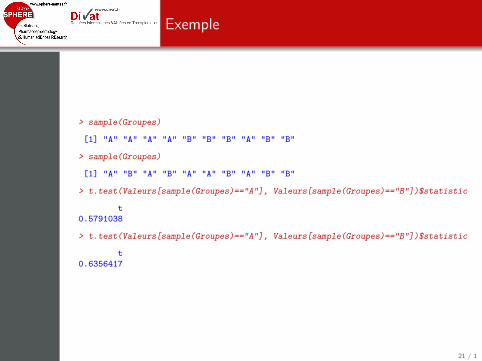
> sample(Groupes)

[1] "A" "A" "A" "A" "B" "B" "B" "A" "B" "B"

> sample(Groupes)

[1] "A" "B" "A" "B" "A" "A" "B" "A" "B" "B"

> t.test(Valeurs[sample(Groupes)=="A"], Valeurs[sample(Groupes)=="B"])$statistic

t0.5791038

> t.test(Valeurs[sample(Groupes)=="A"], Valeurs[sample(Groupes)=="B"])$statistic

t0.6356417

21 / 1

Exemple

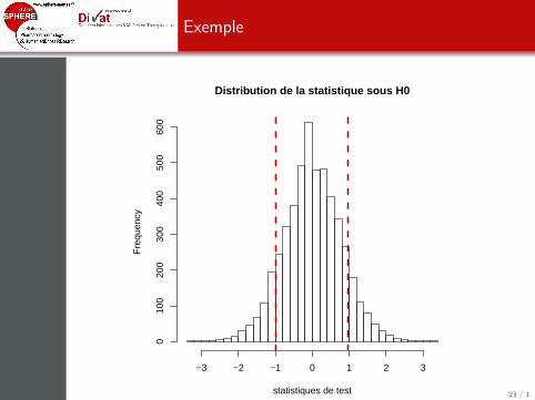
> B<-5000> statistics <- rep(NA, B)> for(b in 1:B)+ {+ statistics[b] <- t.test(Valeurs[sample(Groupes)=="A"],+ Valeurs[sample(Groupes)=="B"])$statistic+ }> hist(statistics, nclass=30, xlab="statistiques de test", main="Distribution de la statistique sous H0")> stat.ini <- t.test(Valeurs[Groupes=="A"], Valeurs[Groupes=="B"])$statistic> abline(v=stat.ini, col="red3", lwd=3, lty=2)> abline(v=-1*stat.ini, col="red3", lwd=3, lty=2)

22 / 1

Exemple

Distribution de la statistique sous H0

statistiques de test

Fre

quen

cy

−3 −2 −1 0 1 2 3

010

020

030

040

050

060

0

23 / 1

Un exemple pour mieux comprendre...

> hist(abs(statistics), nclass=30, xlab="statistiques de test", main="Distribution de la statistique sous H0")> abline(v=abs(stat.ini), col="red3", lwd=3, lty=2)

24 / 1

Exemple

Distribution de la statistique sous H0

statistiques de test

Fre

quen

cy

0.0 0.5 1.0 1.5 2.0 2.5 3.0 3.5

010

020

030

040

050

060

0

25 / 1

Un exemple pour mieux comprendre...

> sum(abs(statistics)>=abs(stat.ini))

[1] 1008

> sum(abs(statistics)>=abs(stat.ini))/B

[1] 0.2016

> t.test(Valeurs[Groupes=="A"], Valeurs[Groupes=="B"])$p.value

[1] 0.3601715

p∗j =

∑Bb=1 I (|t

(b)j | ≥ |tj |)B

= 0.2016

pj = 0.3602 (sans permutation)

26 / 1

Plan

27 / 1

Correction de Bonferroni

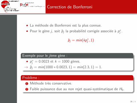
� La methode de Bonferroni est la plus connue.

� Pour le gene j , soit pj la probabilite corrigee associee a p∗j .

pj = min(kp∗j , 1)

Exemple pour le j eme gene :

� p∗j = 0.0023 et k = 1000 genes.

→ pj = min(1000 ∗ 0.0023, 1) = min(2.3, 1) = 1.

Probleme :

1 Methode tres conservative.

2 Faible puissance due au non rejet quasi-systematique de H0.

28 / 1

Procedure de Holm

� Procedure de Holm moins conservative

� Idee :

� Ordonner les genes selon les probabilites critiques.� A chaque fois qu’un test est significatif, le gene suivant est

inclus.� La probabilite critique du gene inclus est corrigee selon le

nombre de genes restant a inclure.

� Posons pr1 ≤ pr2 ≤ ... ≤ prk , les probabilites critiques ordonneesen utilisant les valeurs obtenues par permutation(p∗j , j = 1, 2, ..., k) :

pr1 = kpr1

prj = max(pr(j−1), (k − j + 1)prj) pour 2 ≤ j ≤ k

� Les probabilites critiques superieures a 1 sont corrigees a 1.

29 / 1

Exemple

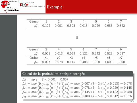
Genes 1 2 3 4 5 6 7p∗j 0.122 0.001 0.523 0.013 0.029 0.987 0.342

⇓

Genes 2 4 5 1 7 3 6p∗j 0.001 0.013 0.029 0.122 0.342 0.523 0.987

Ordre r1 r2 r3 r4 r5 r6 r7prj

0.007 0.078 0.145 0.488 1.000 1.000 1.000

Calcul de la probabilite critique corrigee

pr1 = kpr1 = 7× 0.001 = 0.007pr2 = max(pr(j−1), (k− j + 1)prj) = max(0.007, (7−2 + 1)×0.013) = 0.078pr3 = max(pr(j−1), (k− j + 1)prj) = max(0.078, (7−3 + 1)×0.029) = 0.145pr4 = max(pr(j−1), (k− j + 1)prj) = max(0.145, (7−4 + 1)×0.122) = 0.488pr5 = max(pr(j−1), (k− j + 1)prj) = max(0.488, (7−5 + 1)×0.342) = 1.026

30 / 1

Exemple

Genes 1 2 3 4 5 6 7p∗j 0.122 0.001 0.523 0.013 0.029 0.987 0.342

⇓

Genes 2 4 5 1 7 3 6p∗j 0.001 0.013 0.029 0.122 0.342 0.523 0.987

Ordre r1 r2 r3 r4 r5 r6 r7prj 0.007

0.078 0.145 0.488 1.000 1.000 1.000

Calcul de la probabilite critique corrigee

pr1 = kpr1 = 7× 0.001 = 0.007

pr2 = max(pr(j−1), (k− j + 1)prj) = max(0.007, (7−2 + 1)×0.013) = 0.078pr3 = max(pr(j−1), (k− j + 1)prj) = max(0.078, (7−3 + 1)×0.029) = 0.145pr4 = max(pr(j−1), (k− j + 1)prj) = max(0.145, (7−4 + 1)×0.122) = 0.488pr5 = max(pr(j−1), (k− j + 1)prj) = max(0.488, (7−5 + 1)×0.342) = 1.026

30 / 1

Exemple

Genes 1 2 3 4 5 6 7p∗j 0.122 0.001 0.523 0.013 0.029 0.987 0.342

⇓

Genes 2 4 5 1 7 3 6p∗j 0.001 0.013 0.029 0.122 0.342 0.523 0.987

Ordre r1 r2 r3 r4 r5 r6 r7prj 0.007 0.078

0.145 0.488 1.000 1.000 1.000

Calcul de la probabilite critique corrigee

pr1 = kpr1 = 7× 0.001 = 0.007pr2 = max(pr(j−1), (k− j + 1)prj) = max(0.007, (7−2 + 1)×0.013) = 0.078

pr3 = max(pr(j−1), (k− j + 1)prj) = max(0.078, (7−3 + 1)×0.029) = 0.145pr4 = max(pr(j−1), (k− j + 1)prj) = max(0.145, (7−4 + 1)×0.122) = 0.488pr5 = max(pr(j−1), (k− j + 1)prj) = max(0.488, (7−5 + 1)×0.342) = 1.026

30 / 1

Exemple

Genes 1 2 3 4 5 6 7p∗j 0.122 0.001 0.523 0.013 0.029 0.987 0.342

⇓

Genes 2 4 5 1 7 3 6p∗j 0.001 0.013 0.029 0.122 0.342 0.523 0.987

Ordre r1 r2 r3 r4 r5 r6 r7prj 0.007 0.078 0.145

0.488 1.000 1.000 1.000

Calcul de la probabilite critique corrigee

pr1 = kpr1 = 7× 0.001 = 0.007pr2 = max(pr(j−1), (k− j + 1)prj) = max(0.007, (7−2 + 1)×0.013) = 0.078pr3 = max(pr(j−1), (k− j + 1)prj) = max(0.078, (7−3 + 1)×0.029) = 0.145

pr4 = max(pr(j−1), (k− j + 1)prj) = max(0.145, (7−4 + 1)×0.122) = 0.488pr5 = max(pr(j−1), (k− j + 1)prj) = max(0.488, (7−5 + 1)×0.342) = 1.026

30 / 1

Exemple

Genes 1 2 3 4 5 6 7p∗j 0.122 0.001 0.523 0.013 0.029 0.987 0.342

⇓

Genes 2 4 5 1 7 3 6p∗j 0.001 0.013 0.029 0.122 0.342 0.523 0.987

Ordre r1 r2 r3 r4 r5 r6 r7prj 0.007 0.078 0.145 0.488

1.000 1.000 1.000

Calcul de la probabilite critique corrigee

pr1 = kpr1 = 7× 0.001 = 0.007pr2 = max(pr(j−1), (k− j + 1)prj) = max(0.007, (7−2 + 1)×0.013) = 0.078pr3 = max(pr(j−1), (k− j + 1)prj) = max(0.078, (7−3 + 1)×0.029) = 0.145pr4 = max(pr(j−1), (k− j + 1)prj) = max(0.145, (7−4 + 1)×0.122) = 0.488

pr5 = max(pr(j−1), (k− j + 1)prj) = max(0.488, (7−5 + 1)×0.342) = 1.026

30 / 1

Exemple

Genes 1 2 3 4 5 6 7p∗j 0.122 0.001 0.523 0.013 0.029 0.987 0.342

⇓

Genes 2 4 5 1 7 3 6p∗j 0.001 0.013 0.029 0.122 0.342 0.523 0.987

Ordre r1 r2 r3 r4 r5 r6 r7prj 0.007 0.078 0.145 0.488 1.000 1.000 1.000

Calcul de la probabilite critique corrigee

pr1 = kpr1 = 7× 0.001 = 0.007pr2 = max(pr(j−1), (k− j + 1)prj) = max(0.007, (7−2 + 1)×0.013) = 0.078pr3 = max(pr(j−1), (k− j + 1)prj) = max(0.078, (7−3 + 1)×0.029) = 0.145pr4 = max(pr(j−1), (k− j + 1)prj) = max(0.145, (7−4 + 1)×0.122) = 0.488pr5 = max(pr(j−1), (k− j + 1)prj) = max(0.488, (7−5 + 1)×0.342) = 1.026

30 / 1

Remarque : l’interet d’une filtration prealable

� Objectif : limiter le nombre de genes candidats.

pr1 = kpr1

prj = max(pr(j−1), (k − j + 1)prj) pour 2 ≤ j ≤ k

� La correction diminue quand k diminue.

� Methodes couramment rencontrees :

� Elimination des genes ayant de trop faible ou de trop fortcoefficient de variation.

� Elimination des genes qui ont trop d’individus au-dessus d’uncertain seuil.

31 / 1

Plan

32 / 1

Les donnees †

� 128 patients avec un diagnostic de leucemie aiguelymphoblastique (ALL).

� Des puces contenant l’expression de 12625 genes ont etecollectes.

� Objectif de l’exemple : Identifier les genes qui sont associes a lareponse therapeutique des patients.

†. S. Chiaretti et al. Gene expression profile of adult T-cell acute lymphocyticleukemia identifies distinct subsets of patients with different response totherapy and survival. Blood, 2004, Vol. 103, No. 7 33 / 1

Les analyses sous R

> library(Biobase)> library(multtest)> library(ALL)> library(genefilter)> data(ALL)> dim(exprs(ALL))

[1] 12625 128

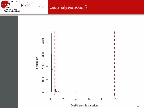
> X<-exprs(ALL)> pheno<-pData(ALL)> coef.var<-function(x) {sd(x)/abs(mean(x))}> coef.var.vector<-apply(2^X, 1, coef.var)> hist(coef.var.vector, nclass=30, xlab="Coefficients de variation",+ main="", xlim=c(0, 10.5))> abline(v=0.7, col="red3", lwd=3, lty=2)> abline(v=10, col="red3", lwd=3, lty=2)

34 / 1

Les analyses sous R

Coefficients de variation

Fre

quen

cy

0 2 4 6 8 10

010

0020

0030

0040

00

35 / 1

Les analyses sous R

> sum(coef.var.vector<=0.7)/length(coef.var.vector)

[1] 0.926495

> sum(coef.var.vector>10)/length(coef.var.vector)

[1] 0

> ffun<-filterfun(pOverA(p=0.2, A=100), cv(a=0.7, b=10))> filt<-genefilter(2^X, ffun)> sum(filt)

[1] 431

> mb<-as.character(pheno$mdr)> table(mb)

mbNEG POS101 24

> filtX<-X[filt,!is.na(mb)]> dim(filtX)

[1] 431 125

> mb <- mb[!is.na(mb)]> length(mb)

[1] 125

36 / 1

Les analyses sous R

> mb.boot<-MTP(X = filtX, Y=mb, test = "t.twosamp.equalvar", robust=TRUE, alpha=c(0.05), B = 100, get.cutoff = TRUE)

running bootstrap...iteration = 100

> sum(mb.boot@rawp<=0.05)/sum(filt)

[1] 0.0324826

> sum(mb.boot@adjp<=0.05)/sum(filt)

[1] 0

> plot(mb.boot@rawp, mb.boot@adjp, ylim=c(0,1), xlim=c(0,1), xlab="P-values non corrigees", ylab="p-value corrigees")> abline(v=0.05, col="red3", lty=2, lwd=2)> abline(h=0.05, col="red3", lty=2, lwd=2)

37 / 1

Les analyses sous R

●● ●● ●● ●●● ●●●● ●●●● ●● ●●● ●● ● ●●●●●● ● ●● ● ●● ●● ●●●

●

●●● ●● ●● ●● ●●●●● ●●● ●● ● ●●● ●●●● ● ●● ●●●●●●● ●●●● ● ●● ● ●●● ●●● ●● ●●● ●● ●● ● ●●●●●●●● ● ● ●● ●

●

●● ● ● ●● ● ●●● ● ●●● ●●● ● ●● ●● ●●●● ●● ●● ●●●● ●● ● ●●●● ●● ● ●●● ●● ● ●● ● ●●●● ●● ●●●● ● ● ●●● ●●● ●●● ●● ● ● ●●●● ● ●●● ●● ●●● ●● ● ● ●●● ●●● ●●● ● ● ●●● ●● ●● ●●● ●● ●●●● ●● ● ●●

●

● ●●●● ●● ●●● ● ● ●●● ●● ● ●● ● ● ●● ●● ● ●●● ●●● ● ●● ● ●●● ● ●● ●● ●● ● ● ●● ● ●●

●● ● ● ●●● ●●●●

● ●●● ● ●●●● ●● ●

●

● ● ● ●● ●● ●● ●● ●● ●●● ●● ● ●●●● ●● ●● ●● ● ●● ●

●

● ● ●●● ● ●● ●●● ●● ●● ●●●● ● ●●● ● ●●● ● ●●● ●● ●●●● ● ● ●●● ●● ●● ● ● ●●●●● ● ●● ●●● ●● ●● ●● ●● ●●● ● ●●

0.0 0.2 0.4 0.6 0.8 1.0

0.0

0.2

0.4

0.6

0.8

1.0

P−values non corrigées

p−va

lue

corr

igée

s

38 / 1

Plan

39 / 1

Limites

� Ne prend pas en compte la structure de dependance des genes

→ Algorithme de Westfall et Young. ‡

� Meme apres permutations et corrections, les probabilites critiquessont peu fiables

→ Cette methode permet de retrouver des resultats plus realistes etde classer les genes en fonction de leur potentiel interet.

� Survol de la methode MTP : nombreuses autres possibilites.

� Apres classement/selection des genes par MTP :

1 Calcul d’une taille d’echantillon minimale necessaire pour unevalidation externe

2 Methodes de mesure specifique des expressions descaracteristiques (PCR, etc.)

3 On retrouve une situation acceptable pour l’utilisation desmethodes statistiques :

Nombre variables <<< Nombre de sujets

‡. Resampling-based multiple testing. Peter H. Westfall, S. Stanley Young,Wiley, New York, 1993 40 / 1