LES and RANS Analysis of the End-Wall Flow in a Linear LPT ...

LES and RANS Analysis of the End-Wall Flow in a Linear LPT Cascade, Part I: Flow and Secondary

Vorticity Fields Under Varying Inlet Condition

Richard PichlerYaomin Zhao

Richard Sandberg*

Dept. of Mechanical EngineeringUniversity of Melbourne

Parkville, Victoria 3010, [email protected]

Vittorio MichelassiBaker Hughes, a GE Company

Via Felice Matteucci 10,50127, Florence, Italy

[email protected]

Roberto PaccianiMichele Marconcini

Andrea ArnoneDept. of Industrial Engineering

University of Florencevia di Santa Marta, 3, 50139 Florence, Italy

[email protected]

ABSTRACT

In low-pressure-turbines (LPT) around 60-70% of losses are generated away from end-walls, while the remaining 30-40% is controlled by the

interaction of the blade profile with the end-wall boundary layer. Experimental and numerical studies have shown how the strength and penetration of

*Corresponding author

TURBO-19-1065 1 Sandberg

the secondary flow depends on the characteristics of the incoming end-wall boundary layer. Experimental techniques did shed light on the mechanism

that controls the growth of the secondary vortices, and scale-resolving CFD allowed to dive deep into the details of the vorticity generation. Along these

lines, this paper discusses the end-wall flow characteristics of the T106 LPT profile at Re=120K and M=0.59 by benchmarking with experiments and

investigating the impact of the incoming boundary layer state. The simulations are carried out with proven Reynolds-averaged Navier–Stokes (RANS)

and large-eddy simulation (LES) solvers to determine if Reynolds Averaged models can capture the relevant flow details with enough accuracy to drive

the design of this flow region.

Part I of the paper focuses on the critical grid needs to ensure accurate LES, and on the analysis of the overall time averaged flow field and

comparison between RANS, LES, and measurements when available. In particular, the growth of secondary flow features, the trace and strength of the

secondary vortex system, its impact on the blade load variation along the span and end-wall flow visualizations are analysed. The ability of LES and

RANS to accurately predict the secondary flows is discussed together with the implications this has on design.

INTRODUCTION

In low-pressure-turbines (LPT) at design point around 60-70% of losses are generated away from end-walls, while the remaining 30-40% is

controlled by the interaction of the blade profile with the end-wall boundary layer. At off-design conditions, end-wall losses may grow above the

percentage indicated above, especially for highly loaded LPT designs often sought after by engine designers to reduce weight and cost.

Due to the presence of the end-wall a vortex system forms and the general flow topology has been summarized by, for example, Sieverding [1]

and Langston [2]. Upstream of the leading edge the end-wall boundary layer separates due to the potential flow field induced by the blade, causing the

formation of a horseshoe vortex with two legs stretching along the suction and pressure sides respectively as discussed by Langston [3]. The potential

flow field in the passage causes a cross flow that moves the pressure-side leg of the horseshoe vortex away from the pressure side and eventually hits the

suction side further downstream (passage vortex). For the suction side leg, two scenarios have been reported. Based on measurements of mass transfer,

Goldstein and Spores [4] proposed that the suction leg travels next to the passage vortex. In contrast Sieverding and Bosche [5] as well as Wang et

al. [6] observed in flow visualization experiments that the suction leg wraps around and merges with the passage vortex. In addition a vortex located

above the passage vortex close to the suction side with opposite rotation to the passage vortex, referred to as counter vortex, has been reported in several

studies. While Langston [3] proposed that the counter vortex originated from the suction side vortex close to the end-wall, Hodson and Dominy [7] as

well as Wang et al. [6] argued that the formation of the counter vortex was due to the skew of the blade surface boundary layer and the strong passage

vortex.

Hermanson and Thole [8] suggested that the differences in the vortex systems discussed above might be due to different inlet conditions and

showed a significant variation of the end-wall flow when comparing uniform inlet profiles to realistic combustor exit profiles for a high pressure turbine


vane. Studies summarized in Vera et al. [9] suggest that the end-wall boundary layer in an LPT is transitional as a result of the boundary layer restarting

downstream of the passage vortex, a conjecture that has been the motivation for comparing laminar and turbulent end-wall boundary layer profiles.

De la Rosa Blanco et al. [10] conducted experiments of two low-speed LPT cascades and used a thin laminar, a thin turbulent and a thick turbulent

end-wall boundary layer. They investigated the stagnation pressure loss in a traverse plane downstream of the cascade and skin friction on the end-wall.

A laminar boundary layer resulted in a larger separation at the end-wall upstream of the leading edge compared to the case with a turbulent boundary

layers, two separate vortex cores in the stagnation pressure loss profile as opposed to one in case of the turbulent boundary layer and the loss cores

being closer to the end-wall for the laminar case.

With the rise of computer power, eddy resolving simulations of low pressure turbines including end-walls have become affordable. Koschichow et

al. [11] simulated an LPT passage with end-wall and studied in particular the impact of an incoming wake on the instantaneous flow field. Cui [12, 13]

used LES to investigate the influence of different boundary layer states as well as an incoming wake on the flow features in the passage and discussed

the influence on loss generation.

In the current work simulations of the T106 LPT profile with parallel end-walls at Re=120K and M=0.59, as described in the experimental setup

of Duden and Fottner [14], are conducted. This experimental study has been chosen as a reference since it represents an engine-like combination of

Mach and Reynolds number, however, the description of the inlet boundary layer state is incomplete. Since it is well known that the inlet boundary

layer state might have a severe influence on the flow, two different inlet boundary layer states are simulated here and compared to understand the

uncertainties associated with the boundary layer specification. The simulations are carried out by both RANS, due to its persisting role as the design

verification workhorse, and highly resolved LES to determine whether Reynolds Averaged models can capture the relevant flow details with a degree of

accuracy able to drive the design of this crucial flow region. Although RANS accuracy is overall good, the remaining deviation from measurement data

is scrutinized with the help of the LES that provides a much deeper insight into the flow field. Part I of the paper focuses on the flow field aerodynamics,

in particular the growth of the secondary flow, the trace and strength of the secondary vortex system, its impact on the blade load variation along the

span, and the decay of the secondary vortex downstream of the trailing edge, a key parameter to determine carry-over effects on adjacent blade rows.

The ability of LES and RANS to predict the secondary flows is discussed together with the implications on design.

NUMERICAL METHODS

Large Eddy simulation

HiPSTAR is a University of Melbourne in-house multi-block structured compressible Navier–Stokes solver purposely developed and optimized

to exploit the latest massively parallel high- performance computing systems. HiPSTAR is a multi-block compressible Navier-Stokes solver that uses

fourth-order accurate finite difference schemes in the spatial domain. Here, only a short summary of the key features of the numerical method are given


as a comprehensive presentation of the code and its performance can be found in Sandberg et al. [15] and Michelassi et al. [16]. In the current study,

derivatives in all three spatial directions are computed using fourth-order accurate explicit central finite-difference schemes with energy-preserving

fourth-order accurate boundary schemes [17]. To ensure the accuracy of the implementation the code has been tested on several canonical cases, most

notably a linear LPT cascade midspan section [15]. At all walls (blade and end-walls) adiabatic no slip boundary conditions have been used whereas

the inlet was specified through a Riemann invariant boundary condition, and at the outlet a zonal characteristic boundary condition was employed [18].

For cases where inlet turbulence was prescribed a digital filtering technique has been used that is based on [19, 20] as discussed in more detail in Pichler

et al. [21]. Statistical averaging is performed in time and about the symmetry plane (center plane). All temporal averages have been conducted using

Favre averaging as described in Wilcox [22].

The axial-pitchwise grids used in this study have been taken from Pichler et al. [23] where the baseline mesh and the fine mesh have 274,176 (G1

in ref. [23]) and 581,760 (G2 in ref. [23]) points, respectively. Both grids have been designed with the aim to resolve most of the turbulence such

that the contribution of the LES subgrid scale model is minimal. The spanwise resolution is designed to have an end-wall normal spacing of less than

1.5 in terms of plus units (z+) in the entire domain and at least 150 points are available across the end-wall boundary layers with a total of 855 points

in the spanwise direction. Hence, the total number of points for the baseline and fine simulations are 234 Million and 497 Million respectively. The

simulations have been conducted on a GPU system (NVIDIA P100) where 30 flow-trough times took 100 hours on 21 GPUs and 83 hours on 53 GPUs

for the baseline and fine cases, respectively. Exploiting the spanwise symmetry about the midplane, averaging of the statistics was performed both in

time and about the symmetry plane to obtain convergence in about 30 flow-through times.

RANS

The TRAF code (Arnone [24]) was selected for the complementary RANS investigations. The code solves the unsteady, three-dimensional,

Reynolds-averaged Navier-Stokes equations in a finite volume formulation on multi-block structured grids. Convective fluxes are discretized by a

2nd-order accurate TVD-MUSCL strategy build on Roe’s up- wind scheme. A central difference scheme is used for the viscous fluxes. The transition

modelling is handled by coupling the widely- used γ−Reθ ,t model proposed by Langtry and Menter [25] to the Wilcox k−ω turbulence model [22]. The

transition model couples an intermittency and a transition-onset Reynolds number transport equation to obtain a dynamic description of the transition,

which makes use of local variables only [26].

The computational domain was discretized using an O-H grid with 621× 101× 161, and 81× 121× 161 mesh points respectively, for a total of

about 11.5 million cells. The mesh was selected on the basis of previous grid-dependence analyses. The y+ values of the mesh nodes closest to the wall

are below 0.3 along the whole blade surface. The z+ values range between 0.2 and 0.5 along the endwall surface.


TESTCASE

The aim of this study is to investigate the end-wall flow field in a linear low pressure turbine cascade using RANS and LES at a realistic Mach

and Reynolds number combination. To understand the accuracy of the simulations it is of interest to compare against experiments. For the targeted

Reynolds number and Mach number range there are only a few reported studies available. The study of Duden and Fottner [14] has been chosen as

the best compromise between a realistic Reynolds (120,000) and Mach number (0.59) on the one hand, and affordability of several cases for a high

resolution LES study on the other hand. The blade profile is the T106A with a pitch to chord ratio of 0.799 and a span to chord ratio (aspect ratio) of 3.

The inlet flow angle is 127.7 degree with respect to the pitchwise direction. The shortcoming of the experimental study is that the inlet boundary layer

state has only been reported in terms of boundary layer thickness, displacement thickness and momentum thickness. While some studies provide more

detailed information like the mean flow profile and one rms profile in the wall normal direction, the authors are not aware of an end-wall flow study in

which the (turbulent) state of the boundary layer is fully characterized and includes information on anisotropy and length scales.

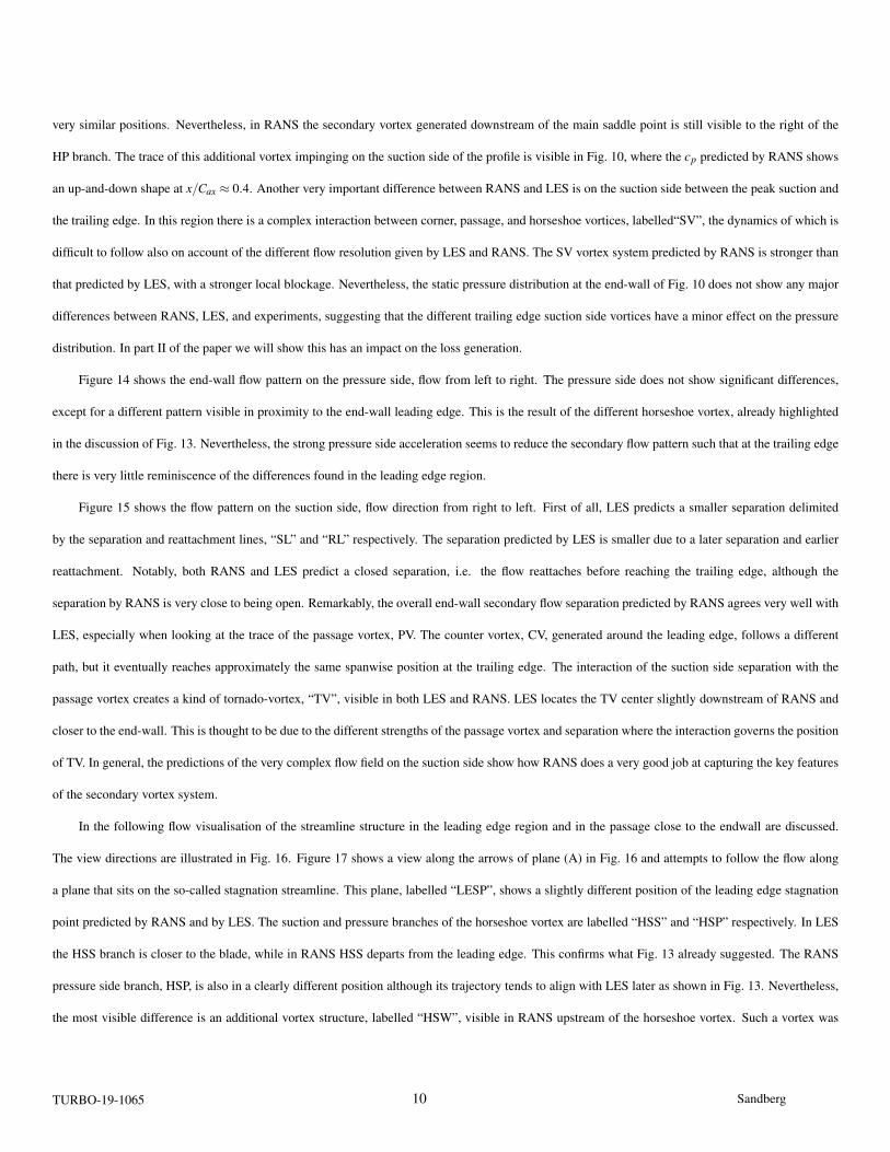
In Fig 1 the computational domain used for the LES is visualized where x, y and z are the axial, pitchwise and spanwise directions, respectively.

If not otherwise stated all lengths are nondimensionalized with the chord length. The leading edge is located at (0,0), the inlet is at x = −0.8 and the

outlet is at x = 2.4.

As mentioned above, the exact profile of the end-wall boundary layer for the reference experiment by Duden and Fottner [14] was not reported.

However, the boundary layer used by Ciorciari, Kirik and Niehus [27] in a study in the same wind tunnel at a slightly lower Reynolds number featured

similar boundary layer parameters as in [14], and therefore their profile is used in the current study. Considering the sensitivity of the flow to the

inlet end-wall boundary layer another LES was also conducted with a second boundary layer state. Comparing the displacement thickness, momentum

thickness and shape factor reported by Duden [14] to zero pressure gradient turbulent boundary layer data, the momentum thickness Reynolds number

would be far in excess of 10,000 which characterizes a fully turbulent zero pressure gradient boundary layer. Since in a real engine the boundary layer

is considered transitional (e.g. Vera et al.[9]), one more LES wtih an inlet boundary layer with a lower momentum thickness Reynolds number was

performed to both estimate the uncertainties in the resulting flow due to the inlet condition and to investigate a more realistic inlet boundary layer. Data

for this lower momentum thickness BL has been taken from an LES study of a zero pressure gradient boundary layer by Eitel-Amor et. al [28]. Both

boundary layers have been fitted to match the inlet boundary layer thickness of the other cases. The cases using the inlet boundary layer profiles by

Eitel-Amor et. al [28] or Ciorciari [27] will be referred to as C2.


RESULTS

Grid convergence

To understand the quality of the solution first a grid convergence study has been conducted. This preparatory study has been conducted using the

end-wall boundary layer profile of case C1, however, at midspan no inflow turbulence has been prescribed such that the results in this section differ

from the ones reported later. Considering that the grid requirement in the freestream is well understood [23], this is not considered a limitation. For the

discretization schemes used in HiPSTAR the target values of x+, y+ and z+ for a high-quality LES in a zero pressure gradient turbulent boundary layer

are x+ < 50, y+ < 2 and z+ < 15−20. For the baseline mesh the maximum x+ along the entire blade is below 30 and the fine mesh is about 30% finer.

In the wall normal direction y+ is less than 2.2 at midspan and less than 3 at the end-wall while along most of the blade the values are below 2 and

the fine mesh is about twice as fine reaching y+ < 1 everywhere except for the last 10% on the pressure side. In the spanwise direction the grid used

satisfies the required values discussed in [23] at the midspan section to provide grid-independent results of the Reynolds stress such that a refinement

study was not necessary. At the end-wall the target grid is inspired by DNS values as can be seen in Fig. 2 such that it is expected to suffice for an LES.

For the RANS simulations this study relied on the guideline values developed in numerous previous studies.

The influence of the grid on the solution is first assessed by the pressure distribution around the blade, defined as [14]

cp =p(x)− pout,mix, f ree

pt,in, f ree − pout,mix, f ree(1)

where pt,in, f ree is the freestream stagnation pressure at the inlet and pout, f ree is the mixed-out static pressure at the outlet, illustrated in Fig. 3. Only

close to the wall minor variations between the two grids can be seen but overall the agreement is excellent. Also, the solution qualitatively captures the

trend of the pressure distribution seen in the experiment.

Since it also incorporates viscous effects, vortex shedding and the subsequent mixing of the wake, the total pressure loss downstream of the blade

row shown in Fig. 4 is a more difficult metric to match. The loss coefficient is defined as [14]

ω =pt,in, f ree − pt(x,y,z)

pt,in, f ree − pout,mix, f ree. (2)

Filled contours represent the fine mesh whereas lines indicate the baseline mesh. Again the agreement between the two solutions is good, with only

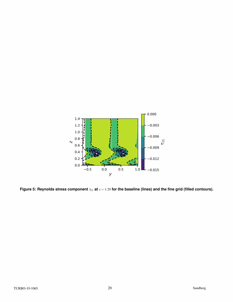
minor variations in the free-stream and in the region between the freestream and the end-wall region. Finally, the resolved Reynolds stresses [22]

depicted in Fig. 5 shows good agreement and the solutions on both grids show a similar levels of resolved Reynolds stress. The resolved Reynolds

stress is comprised of structures of different size where smaller structures carry less energy. Hence, if the sum is virtually the same it means that the

structures that contribute to the Reynolds stress significantly are resolved on both grids and it implies that all quantities of interest to this study are fully

resolved and grid independent.


INFLUENCE OF THE INLET PROFILE

In this section a comparison with the experiment is presented that requires a discussion of the influence of the inlet flow profile since the actual

profile used in the experiment is not fully known. For the LES the inlet profiles are prescribed in terms of the mean velocity profile as well as

the Reynolds stress components available from [28] for case (C1) and for case (C2) the measured [27] values of TKE and velocity magnitude are

prescribed. Turbulence is introduced using the digital filter technique that allows to prescribe length scale as well as intensity in all three directions.

However, since synthetic turbulence is used it needs some length to develop to a real boundary layer profile. Therefore, the flow is characterised in

terms of the mean velocity magnitude (time and pitchwise mixed-out averaged) as well as the turbulence kinetic energy profile close to the leading edge

at x =−0.25Cax, which are shown in Fig. 6. Both profiles have a slightly greater boundary layer thickness as compared to the inlet and the difference

in terms of momentum distribution is obvious. This suggests that C2 might be a profile at substantially larger momentum thickness Reynolds number.

In addition the peak TKE level close to the end-wall is higher in the C2 case, however, the plateau in the outer region of the boundary layer is missing.

The free-stream TKE value is almost the same in both cases and corresponds to a free-stream turbulence intensity of 5.0%(√

2k/3/cloc

)which is

higher than in the experiment (3.5%). The length scale present in the experiment is not provided, thus in the LES it was set to 4% of the chord length

at the inlet based on previous mid-span studies. For the RANS simulations inlet profile C2 is used and prescribed in terms of total temperature, total

pressure and turbulence kinetic energy, where the near wall peak has not been prescribed. However, a small peak develops close to the end-wall and its

magnitude is about half that of the LES. More detailed discussions are presented in part II [29].

The pressure distribution of the two different inlet profiles as predicted by LES are compared to each other and to the experiments at different

locations along the span in Fig. 7 where solid lines as well as dashed lines represent cases C2 and C1, respectively. Directly at the end-wall the two

inlet conditions bracket the experimental values on the suction side up to x/Cax = 0.7 where both cases approach each other and the experiment. At

z/H ≈ 0.01 both cases show similar differences on the entire suction side. At z/H ≈ 0.05 the cp distribution is about midway between the end-wall and

the mid-span ones.

At z/H ≈ 0.14 the pressure distribution shows only minor differences to the midspan profile on the suction side up to peak suction for both cases

and lower cp values downstream.

Notable differences are restricted to downstream of peak suction where the plateau indicating a separation develops when moving away from

the wall. In general the development of the separation and the recovery of the midspan profile occurs at larger spanwise location for case C1 with

respect to case C2. At midspan both inlet conditions give similar pressure distributions, in close agreement with the experiment. On the pressure side

the end-wall profiles with the two different inlets have a different shape up to x/Cax = 0.4 which is due to a larger separation in the C1 case. Again

the experimental values lie between those of the two inlet boundary layers considered here up to x/Cax ≈ 0.6. Close to the trailing edge the pressure

coefficient computed in the simulations is larger than the one measured in the experiment. While neither of the simulations predicts the same details of

the flow, the simulations bracket the experiment suggesting that an inlet profile between the two profiles used would result in the correct solution.


To get a better understanding of the extent of the flow separation, a contour of mean zero skin friction on the suction side for both inlet boundary

layer cases is superimposed on the oil film visualization reported from the experiment (Fig. 8). Skin friction has been computed only considering the

wall shear stress in the tangential direction and omitting the spanwise contribution. The area encircled by the contour has negative mean skin friction

and indicates a separation bubble. At midspan the separation extent of both inlet profile cases is the same, as expected considering the same inlet

turbulence intensity of the incoming flow at midspan. Differences can be seen closer to the end-wall where inlet profile C2 exhibits separation closer

to the end-wall than in case C1. In general, it is expected that the vortex system of the secondary flow suppresses a separation on the suction side due

to the higher mixing of momentum. Hence, this behaviour indicates that the vortex system in case C2 is closer to the end-wall than in case C1. The

agreement of the simulation results with the experiments is reasonable with the experiment showing an earlier separation at midspan and the attached

area close to the end-wall matching case C1.

Stagnation pressure loss ω is presented in Fig. 9 where the top part shows a 2D map aligned with the pitchwise and spanwise direction. Filled

contours represent case C1 and the solid lines show case C2. At midspan both cases have a similar loss shape as expected since the flow in the midspan

is not affected by the end-wall. The elevated stagnation loss areas at (y,z)≈ (−0.5,0.4) are related to secondary vortices, namely the passage and the

counter vortex. As suggested above the fuller velocity profile results in the secondary vortices being closer to the end-wall which is confirmed by the

stagnation pressure loss plots. Close to the end-wall the flow wake is wider for the C1 case and it seems that at around z = 0.05 the pitchwise location

is shifted towards lower values indicating a larger turning at that height. The pitchwise mass-averaged stagnation pressure loss is presented in Fig. 9

(bottom) and it is obvious that the stagnation pressure loss coefficient is higher for case C1. Note that this is due to the definition of the stagnation

pressure loss that does not account for the momentum deficit in the endwall boundary layer which is larger for C1 compared to C2. Hence, part of the

additional loss might be due that effect. When comparing the simulations to the experiment both simulations show higher losses at midspan that might

be caused by the different inlet turbulence conditions. From z = 0 to z = 0.2 the agreement between case C2 and the experiment is good and case C1

shows a higher loss. The peak in loss due to the secondary vortices is at z=0.38, 0.41 and 0.42 for C2, the experiment and C1 respectively. Again,

the experiment is between the results from the two inlet boundary layer locations. However, the peak loss magnitudes in both simulations is higher

than in the experiment. Overall, the agreement is reasonable with regard to the uncertainty in the inlet boundary condition. In part II [29] additional

comparisons with the experiment are presented.

COMPARISON BETWEEN RANS AND LES

Pressure distributions of RANS and LES using inlet C2 are compared in Fig. 10 at different spanwise locations. At the end-wall the pressure

distribution on the suction side obtained with RANS shows some variations around x/Cax 0.4 which is approximately the location where the passage

vortex reaches the suction side as will be shown later. Overall, though, the agreement is good. At z/H = 10% both profiles are virtually on top of each


other and only close to the trailing edge the pressure coefficient recovers faster in the RANS. Also at midspan the agreement between the two methods

is good. On the pressure side there is virtually no difference between the RANS or LES solutions.

The skin friction coefficient c f for both methods is presented in Fig. 11. On the pressure side both solutions are in good agreement. Differences

can be seen for the suction side where the differences are larger for profiles closer to the end-wall. At midspan only the post-separation behaviour is

different and it appears as if the LES is closer to reattachment as will be shown later. At z/H = 10% the LES simulation almost predicts separation and

then picks up in skin friction again which might indicate transition. This behaviour might indicate an intermittent separation (e.g. [21]). The RANS

clearly does not separate, however, the skin friction does not grow to values comparably to the LES. At z/H = 5% the behaviour over most of the

suction side is the same except for the region around x/Cax ≈ 0.65 where skin friction in the LES does not increase as much in the beginning but then

shows a more pronounced peak than the RANS simulation.

In Fig. 12 the mass averaged flow angle evolution downstream of the trailing edge is displayed. RANS and LES with the same inlet profile C2

show reasonable agreement at all axial locations. In general the RANS computes a lower turning close to the end-wall (z/H < 0.05) followed by a

higher turning up to the minimum location. The minimum in the RANS is slightly further away from the end-wall and also the midspan value is reached

at higher z/H values. With respect to the differences between LES and RANS the difference between the LES solutions at different inlet conditions

is significantly larger and the deviations from the midspan value is larger both in terms of minimum and maximum. The experimental value again is

between the LES solutions with different inlet conditions suggesting that the inlet in the experiment is between those two values.

Flow visualizations

This section compares the surface flow on the end-walls predicted by RANS and LES. Figure 13 shows the end-wall flow details. The same

figure shows the pressure distribution contours. While the general flow patterns from LES and RANS are quite similar there are some differences in

the details. The saddle point“SaP” identifies the location where the two branches of the horseshoe vortex splits to the pressure and suction side [30].

RANS and LES predict very similar locations of SaP, indicating that the two approaches predict very similar profile leading edge potential effects.

Although the simulations used the same inlet velocity and turbulent kinetic profiles, RANS predicts a more complex flow pattern as compared with

LES. While this will be further discussed in the analysis of the stagnation plane, here it is evident that downstream of the saddle point LES shows one

single horseshoe vortex core, while RANS predicts an additional separation line that highlights the presence of a secondary end-wall vortex (SaP1). As

discussed by [12] several vortices are also present in the instantaneous snapshots, however, since they move around and average out only the one at the

leading edge remains in the time-averaged data. This result highlights a potential risk in the simulations as RANS and LES may react differently to the

same inlet profile. Nevertheless, the additional stagnation line in the mean flow field predicted by RANS remains confined and does not have any major

impact on the flow field. This is confirmed by the position of the pressure side branch of the horseshoe vortex (HP), which LES and RANS predict at


very similar positions. Nevertheless, in RANS the secondary vortex generated downstream of the main saddle point is still visible to the right of the

HP branch. The trace of this additional vortex impinging on the suction side of the profile is visible in Fig. 10, where the cp predicted by RANS shows

an up-and-down shape at x/Cax ≈ 0.4. Another very important difference between RANS and LES is on the suction side between the peak suction and

the trailing edge. In this region there is a complex interaction between corner, passage, and horseshoe vortices, labelled“SV”, the dynamics of which is

difficult to follow also on account of the different flow resolution given by LES and RANS. The SV vortex system predicted by RANS is stronger than

that predicted by LES, with a stronger local blockage. Nevertheless, the static pressure distribution at the end-wall of Fig. 10 does not show any major

differences between RANS, LES, and experiments, suggesting that the different trailing edge suction side vortices have a minor effect on the pressure

distribution. In part II of the paper we will show this has an impact on the loss generation.

Figure 14 shows the end-wall flow pattern on the pressure side, flow from left to right. The pressure side does not show significant differences,

except for a different pattern visible in proximity to the end-wall leading edge. This is the result of the different horseshoe vortex, already highlighted

in the discussion of Fig. 13. Nevertheless, the strong pressure side acceleration seems to reduce the secondary flow pattern such that at the trailing edge

there is very little reminiscence of the differences found in the leading edge region.

Figure 15 shows the flow pattern on the suction side, flow direction from right to left. First of all, LES predicts a smaller separation delimited

by the separation and reattachment lines, “SL” and “RL” respectively. The separation predicted by LES is smaller due to a later separation and earlier

reattachment. Notably, both RANS and LES predict a closed separation, i.e. the flow reattaches before reaching the trailing edge, although the

separation by RANS is very close to being open. Remarkably, the overall end-wall secondary flow separation predicted by RANS agrees very well with

LES, especially when looking at the trace of the passage vortex, PV. The counter vortex, CV, generated around the leading edge, follows a different

path, but it eventually reaches approximately the same spanwise position at the trailing edge. The interaction of the suction side separation with the

passage vortex creates a kind of tornado-vortex, “TV”, visible in both LES and RANS. LES locates the TV center slightly downstream of RANS and

closer to the end-wall. This is thought to be due to the different strengths of the passage vortex and separation where the interaction governs the position

of TV. In general, the predictions of the very complex flow field on the suction side show how RANS does a very good job at capturing the key features

of the secondary vortex system.

In the following flow visualisation of the streamline structure in the leading edge region and in the passage close to the endwall are discussed.

The view directions are illustrated in Fig. 16. Figure 17 shows a view along the arrows of plane (A) in Fig. 16 and attempts to follow the flow along

a plane that sits on the so-called stagnation streamline. This plane, labelled “LESP”, shows a slightly different position of the leading edge stagnation

point predicted by RANS and by LES. The suction and pressure branches of the horseshoe vortex are labelled “HSS” and “HSP” respectively. In LES

the HSS branch is closer to the blade, while in RANS HSS departs from the leading edge. This confirms what Fig. 13 already suggested. The RANS

pressure side branch, HSP, is also in a clearly different position although its trajectory tends to align with LES later as shown in Fig. 13. Nevertheless,

the most visible difference is an additional vortex structure, labelled “HSW”, visible in RANS upstream of the horseshoe vortex. Such a vortex was


visible in Fig. 13 as well, but Fig. 17 shows that it remains distinct from both HSS and HSP. Therefore, the different HSS and HSP paths predicted by

RANS compared to LES should not be attributed directly to the presence of HSW, but rather to the different end-wall boundary layer upstream HSP

and HSS seen in RANS as a consequence of HSW.

In Figs. 18 and 19 mean flow streamlines are presented for the C1 and C2 case, respectively. The view direction is along the blue arrows, see

Fig. 16. A view from the back onto the cascade is presented where the normal vector pointing out of the plane is the mean flow direction. Two

subsequent trailing edges are labelled TE1 and TE2 and the blade’s opacity has been set to 0.5 such that the streamlines evolution through the passage

can be seen. Streamlines have been seeded along pitchwise lines at x = 0. (LE) and different spanwise heights z = 0.01, z = 0.06, z = 0.12, z = 0.2,

z= 0.3 and z= 0.4 that are labelled (a), (b), (c), (d), (e), and (f), respectively. Hence, streamlines of the same seed form a streamsurface that contains the

flow that passed through the same spanwise height of the end-wall boundary layer at x = 0.. Note that the seeding extent along the pitchwise direction

has been set to cover all the streamlines in the passage between TE1 and TE2. However, the seeding does not provide all the streamlines through the

neighbouring passages such that the discussion will be limited to the passage between TE1 and TE2.

Looking at the stream surfaces at the exit allows to understand the relocation of the incoming end-wall boundary layer. At midspan flow to the left

of the stagnation plane shown in Fig. 17 wraps around the leading edge flow along the suction side whereas those to the right of the suction side remains

and moves along the pressure side. Close to the end-wall though, the passage vortex interacts with the near wall flow such that most of it ends up close

to the suction side as can be seen when looking at the brown streamlines in Fig. 18, representing the end-wall boundary layer at the inlet. While the flow

to the left of the stagnation surface follows a similar path as in the midspan region, the flow to the right is divided by two mechanisms. Flow closest

to the end-wall is deflected and crosses the passage upstream of the passage vortex as can be seen in 17. Flow further away, but still close enough to

the passage vortex, wraps around the vortex and merges with the passage vortex. Hence, the near end-wall flow at the inlet follows the passage vortex

that moves across the passage until it reaches the suction side as discussed above. The extent of flow that interacts with the passage vortex depends

on the inlet condition, as can be seen in Figs. 18 and 19. In both cases the near wall layer (brown) mostly is deflected and ends up to the left of the

passage vortex. The following streamline layers of the inlet boundary layers visualized wrap around the passage vortex up to a spanwise coordinate

of ≈ 0.2 and ≈ 0.12 for cases C1 and C2, respectively. Considering that the boundary layer thickness at the inlet is 0.26 in cases C1 ≈ 75% of the

inlet end-wall boundary layer ends up in the passage vortex. For case C2 still about 50% of the inlet endwall boundary layer rolls up into the passage

vortex. Considering that the stagnation pressure loss is based on constant reference values for all regions and that the inlet endwall boundary layer in

general has a momentum deficit, the actual loss in the core might be overestimated, in particular when comparing losses between cases with different

inlet boundary layer momentum thickness deficit. A detailed analysis of the loss generation can be found in part II [29].


CONCLUSIONS

LES and RANS have been conducted of a linear cascade of the well-known T106A low pressure turbine blade. The configuration under investiga-

tion here has parallel end-walls. RANS calculations have been conducted by following very well established grid size best practice rules applicable to

this class of flows. Conversely, LES grid convergence was carefully scrutinized to make sure the end-wall flows were appropriately captured. LES was

used to determine the impact of the inlet boundary layer characteristics on the development and penetration of secondary flows. Such an investigation

is of key importance to designers who are often asked to proceed with uncertainties in the blade row end-wall boundary layer details.

Motivated by the limited description of the end-wall boundary layer state in the reference experiment and to understand the influence of smaller

differences in the inlet boundary layer state as investigated in previous studies, LES solutions of two different turbulent inlet end-wall boundary layers

with the same boundary layer thickness but different momentum thickness have been conducted and investigated. LES showed that while the overall

flow structure did not change with the different inlet conditions, the passage vortex core migration is affected, and consequently the secondary flow

spanwise penetration. Both LES solutions show small deviations from the experimental study but remain generally quite close to the values reported in

the experiments. Also the qualitative agreement with experimental values and overall flow features that have been reported in previous studies is good.

In the 3D design of airfoils, two key prerequisites of a prediction tool are to get the pressure distribution and skin friction right along the span. The

direct comparison of cp predicted by LES and RANS with test data showed a remarkable agreement both at midspan and at the endwall. Also, the skin

friction coefficient from RANS is indistinguishable from LES at midspan. Some difference arise at 5% and 10% span after the peak suction position,

i.e. where the pressure gradient switches from favourable to adverse. Notably the reference experiment, RANS and LES agree on the presence of a

suction side separation that reattaches prior to the trailing edge. Although the flow angle was measured quite far downstream, and surely downstream

of the expected position of a downstream blade row, LES remains close to the reference data (further details will be discussed in part II).

The flow visualization revealed some local differences between LES and RANS, in particular close to the wall-surfaces where additional vortices

have been found. Nevertheless, these local changes do not significantly affect the global flow topology and downstream of the blade row both methods,

RANS and LES, give similar results. Part I allows to conclude that RANS and LES are able to drive the design substantially in the same direction. Part

II will focus on a more quantitative analysis and will focus on losses.

ACKNOWLEDGEMENTS

The authors gratefully acknowledge Baker Hughes, a GE Company for granting the permission to publish this paper. Compute time for the LES has

been provided by the Pawsey Supercomputing center in Perth, Australia, and the Swiss national supercomputing center CSCS in Lugano, Switzerland.

The work conducted at the University of Melbourne was conducted under a GE research grant.


NOMENCLATURE

C blade chord

c velocity magnitude

cp blade pressure distribution

k turbulence kinetic energy

H span height

l blade surface length

Greek

ω stagnation loss coefficient

τi j Reynolds stress

Subscripts and Superscripts

ax axial

in inlet

is isentropic

f ree freestream

loc local

out outlet

t total quantity

Acronyms

CV counter vortex

EW end-wall

LE leading edge

LES Large eddy simulation

LPT Low pressure turbine

PV passage vortex

TE trailing edge

TKE turbulent kinetic energy


References

[1] Sieverding, C., 1985. “Recent Progress in the Understanding of Basic Aspects of Secondary Flows in Turbine Blade Passages”. J. Eng. Gas Turb.

Power, 107(2), pp. 248–257.

[2] Langston, L., 2001. “Secondary Flows in Axial Turbines – A Review”. Annals of the New York Academy of Sciences, 934(1), pp. 11–26.

[3] Langston, L., 1980. “Crossflows in a Turbine Cascade Passage”. Journal of Engineering for Power, 102(4), pp. 866–874.

[4] Goldstein, R., and Spores, R., 1988. “Turbulent Transport on the Endwall in the Region Between Adjacent Turbine Blades”. ASME J. Heat

Transfer, 110, pp. 862–869.

[5] Sieverding, C., and Van Den Bosche, P., 1983. “The use of Coloured Smoke to Visualize Secondary Flows in a Turbine-Blade Cascade”. J. Fluid

Mech., 134, pp. 85–89.

[6] Wang, H., Olson, S., Goldstein, R., and Eckert, E., 1997. “Flow Visualization in a Linear Turbine Cascade of High Performance Turbine Blades”.

ASME J. Turbomach., 119(1), pp. 1–8.

[7] Hodson, H., and Dominy, R., 1987. “Three-Dimensional Flow in a Low-Pressure Turbine Cascade at Its Design Condition”. ASME J. Turbomach.,

109(2), pp. 177–185.

[8] Hermanson, K. S., and Thole, K. a., 2000. “Effect of Inlet Conditions on Endwall Secondary Flows”. J. Propuls. Power, 16(2), pp. 286–296.

[9] Vera, M., de la Rosa Blanco, E., Hodson, H., and Vazquez, R., 2009. “Endwall Boundary Layer Development in an Engine Representative

Four-Stage Low Pressure Turbine Rig”. ASME Conf. Proc., 131(1), pp. 011017–1 – 011017–9.

[10] de la Rosa Blanco, E., Hodson, H. P., Vazquez, R., and Torre, D., 2003. “Influence of the state of the inlet endwall boundary layer on the interaction

between pressure surface separation and endwall flows”. P. I. Mech. Eng. A-J. Pow., 217(4), pp. 433–442.

[11] Koschichow, D., Fröhlich, J., Kirik, I., and Niehuis, R., 2014. “DNS of the Flow Near the Endwall in a Linear Low Pressure Turbine Cascade

with Periodically Passing Wakes”. In Proc. ASME Turbo Expo 2014, paper GT2014-25071.

[12] Cui, J., Nagabhushana Rao, V., and Tucker, P., 2015. “Numerical Investigation of Contrasting Flow Physics in Different Zones of a High-Lift

Low-Pressure Turbine Blade”. ASME J. Turbomach., 138(1), p. 011003.

[13] Cui, J., Rao, V. N., and Tucker, P. G., 2017. “Numerical investigation of secondary flows in a high-lift low pressure turbine”. Int. J. Heat Fluid

Flow, 63, pp. 149–157.

[14] Duden, A. and Fottner, L., 1997, “Influence of Taper, Reynolds Number and Mach Number on the Secondary Flow Field of a Highly Loaded

Turbine Cascade”. P. I. Mech. Eng. A-J. Pow., 211(4), pp. 309–320.

[15] Sandberg, R., Michelassi, V., Pichler, R., Chen, L., and Johnstone, R., 2015. “Compressible Direct Numerical Simulation of Low-Pressure

Turbines - Part I: Methodology”. ASME J. Turbomach., 137(5).

[16] Michelassi, V., Chen, L.-W., Pichler, R., and Sandberg, R., 2015. “Compressible Direct Numerical Simulation of Low-Pressure Turbines - Part II:


Effect of Inflow Disturbances”. ASME J. Turbomach., 137(7).

[17] Carpenter, M. H., Nordström, J., and Gottlieb, D., 1999. “A Stable and Conservative Interface Treatment of Arbitrary Spatial Accuracy”. J. Comp.

Phys., 148(2), pp. 341–365.

[18] Sandberg, R. D., Jones, L. E., and Sandham, N. D., 2006. “A zonal characteristic boundary condition for numerical simulations of aerodynamic

sound”. In Eur. Conf. Comput. Fluid Dyn. {ECCOMAS CFD} 2006, P. Wesseling, E. Oñate, and J. Périaux, eds.

[19] Klein, M., Sadiki, A., and Janicka, J., 2003. “A digital filter based generation of inflow data for spatially developing direct numerical or large

eddy simulations”. J. Comp. Phys., 186(2), pp. 652–665.

[20] Xie, Z. T., and Castro, I. P., 2008. “Efficient generation of inflow conditions for large-eddy simulation of street-scale flows”. Flow, Turbul.

Combust., 81(3), pp. 449–470.

[21] Pichler, R., Sandberg, R. D., Laskowski, G., and Michelassi, V., 2017. “High-fidelity simulations of a linear hpt vane cascade subject to varying

inlet turbulence”. In Proc. Procedings ASME Turbo Expo 2017 - paper GT2017-63079.

[22] Wilcox, D. C., 1998. Turbulence Modeling for CFD, 2nd ed. DCW Industries.

[23] Pichler, R., Sandberg, R. D., and Michelassi, V., 2016. “Assessment of grid resolution requirements for accurate simulation of disparate scales of

turbulent flow in low-pressure turbines”. In Procedings ASME Turbo Expo 2016 - paper GT2016-56858.

[24] Arnone, A., 1994. “Viscous Analysis of Three–Dimensional Rotor Flow Using a Multigrid Method”. ASME J. Turbomach., 116(3), pp. 435–445.

[25] Langtry, R. B., and Menter, F. R., 2009. “Correlation-Based Transition Modeling for Unstructured Parallelized Computational Fluid Dynamics

Codes”. AIAA J., 47(12), dec, pp. 2894–2906.

[26] Pacciani, R., Marconcini, M., Arnone, A., and Bertini, F., 2014. “Predicting High-Lift Low-Pressure Turbine Cascades Flow Using Transition-

Sensitive Turbulence Closures”. ASME J. Turbomach., 136(5), sep, p. 051007.

[27] Ciorciari, R., Kirik, I., and Niehuis, R., 2013. “Effects of Unsteady Wakes on the Secondary Flows in the Linear T106 Turbine Cascade”. In Proc.

ASME Turbo Expo 2013 - paper GT2013-94768.

[28] Eitel-Amor, G., Örlü, R., and Schlatter, P., 2014. “Simulation and validation of a spatially evolving turbulent boundary layer up to Reθ =8300”.

Int. J. Heat Fluid Flow, 47, pp. 57–69.

[29] Marconcini, M., Pacciani, R., Arnone, A., Michelassi, V., Pichler, R., Zhao, Y., and Sandberg, R., 2019. “Large Eddy Simulation and RANS

Analysis of the End-Wall Flow in a Linear Low-Pressure-Turbine Cascade - Part II: Loss Generation”. ASME J. Turbomach., 141(5), p. 051004.

[30] Contini, D., Manfrida, G., Michelassi, V., and Riccio, G., 2000. “Measurements of vortex shedding and wake decay downstream of a turbine inlet

guide vane”. Flow, Turbul. Combust., 64(4), pp. 253–278.


LIST OF FIGURES

Figure 1: Simulation domain for the LES: block edges are shown. The inlet and outlet planes are indicated and

all open blockfaces are interfaces where those at the pitchwise domain boundary are connected using a

periodic condition. (turbo-19-1065-fig01)

Figure 2: End-wall normal grid spacing of the first cell in plus units (z+) for both grids at different spanwise loca-

tions z for the baseline simulation. (turbo-19-1065-fig02)

Figure 3: Pressure distribution around the blade at different spanwise locations z/H where solid lines denote the

fine simulation and dashed lines denote the baseline simulation. Circles and squares denote the mea-

sured [14] pressure distribution at the end-wall and at midspan, respectively. (turbo-19-1065-fig03)

Figure 4: Total pressure loss at x = 1.29 for the baseline (lines) and the fine grid (filled contours). (turbo-19-1065-fig04)

Figure 5: Reynolds stress component τ11 at x = 1.29 for the baseline (lines) and the fine grid (filled contours). (turbo-

19-1065-fig05)

Figure 6: Pitchwise mixed-out velocity magnitude (top) and pitchwise mass-averaged turbulence kinetic energy

(bottom) close to the inlet at x/Cax =−0.25.

(a) (turbo-19-1065-fig06a)

(b) (turbo-19-1065-fig06b)

Figure 7: Pressure distribution at different spanwise locations for case C1 (dashed) and case C2 (solid). (turbo-19-

1065-fig07)

Figure 8: Comparison of the flow separation extent between the experiment [14], case C1 and C2, where l is the

length along the suction surface measured from the leading edge. (turbo-19-1065-fig08)

Figure 9: Top: Total pressure loss at x/Cax = 1.5 for case C1 (filled contours) and case C2 (lines). Bottom: Pitch

average loss coefficient compared with experiments [14].

(a) (turbo-19-1065-fig09a)

(b) (turbo-19-1065-fig09b)


Figure 10: Pressure distribution comparison between RANS and LES using inlet profile C2 at three different span-

wise positions. (turbo-19-1065-fig10)

Figure 11: Skin friction around the blade - comparison between RANS and LES using inlet profile C2 at three differ-

ent spanwise positions. (turbo-19-1065-fig11)

Figure 12: Pitchwise averaged flow angle with respect to the axial direction along the spanwise direction where

the end-wall is at zero at four locations: (a) x/Cax = 1.03; (b) x/Cax = 1.1; (c) x/Cax = 1.3; (d) x/Cax = 1.5. The

experimental data which is only available at x/Cax = 1.5 is presented with circles. (turbo-19-1065-fig12)

Figure 13: Hub streamlines for LES and RANS. (turbo-19-1065-fig13)

Figure 14: Pressure side streamlines for LES and RANS. (turbo-19-1065-fig14)

Figure 15: Suction side streamlines for LES and RANS. (turbo-19-1065-fig15)

Figure 16: Visualisation of the view directions used to discuss detailed flow features. The view plane labelled (A)

is used to show the leading edge flow patterns and the view plane labelled (B) is used to investigate the

streamlines in the passage. (turbo-19-1065-fig16)

Figure 17: Streamlines in the leading edge region for LES and RANS. (turbo-19-1065-fig17)

Figure 18: Illustration of streamlines for case C1: all streamlines pass through pitchwise line at x = 0 and different

spanwise values of z = 0.01 (a), z = 0.06 (b), z = 0.12 (c), z = 0.2 (d) z = 0.3 (e) and z = 0.4 (f). The view direction

is such that the normal vector out of the plane is the mean flow direction. (turbo-19-1065-fig18)

Figure 19: Illustration of streamlines for case C2: all streamlines pass through pitchwise line at x = 0 and different

spanwise values of z = 0.01 (a), z = 0.06 (b), z = 0.12 (c), z = 0.2 (d) z = 0.3 (e) and z = 0.4 (f). The view direction

is such that the normal vector out of the plane is the mean flow direction. (turbo-19-1065-fig19)


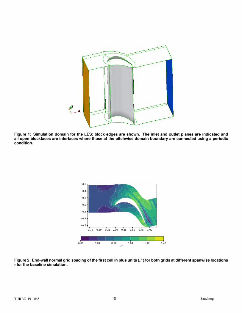
Figure 1: Simulation domain for the LES: block edges are shown. The inlet and outlet planes are indicated andall open blockfaces are interfaces where those at the pitchwise domain boundary are connected using a periodiccondition.

−0.75 −0.50 −0.25 0.00 0.25 0.50 0.75 1.00−0.6

−0.4

−0.2

0.0

0.2

0.4

0.6

0.00 0.28 0.56 0.84 1.12 1.40z +

Figure 2: End-wall normal grid spacing of the first cell in plus units (z+) for both grids at different spanwise locationsz for the baseline simulation.


-0.6

-0.4

-0.2

0.0

0.2

0.4

0.6

0.8

1.0

0.0 0.2 0.4 0.6 0.8 1.0

Cp

x/Cax

EXP 0%

EXP 50%

LES 0%

LES 2%

LES 15%

LES 50%

Figure 3: Pressure distribution around the blade at different spanwise locations z/H where solid lines denote thefine simulation and dashed lines denote the baseline simulation. Circles and squares denote the measured [14]pressure distribution at the end-wall and at midspan, respectively.

0.5 0.0 0.5 1.0y

0.0

0.2

0.4

0.6

0.8

1.0

1.2

1.4

z

0.0

0.1

0.2

0.3

0.4

Figure 4: Total pressure loss at x = 1.29 for the baseline (lines) and the fine grid (filled contours).


0.5 0.0 0.5 1.0y

0.00.20.40.60.81.01.21.4

z

0.015

0.012

0.009

0.006

0.003

0.000

11

Figure 5: Reynolds stress component τ11 at x = 1.29 for the baseline (lines) and the fine grid (filled contours).


0.0

0.1

0.2

0.3

0.4

0.5

0.0 0.1 0.2 0.3 0.4 0.5 0.6

Cm

ix

z

LES C1

LES C2

0.0000

0.0005

0.0010

0.0015

0.0020

0.0025

0.0 0.1 0.2 0.3 0.4 0.5 0.6

km

ass

z

LES C1

LES C2

Figure 6: Pitchwise mixed-out velocity magnitude (top) and pitchwise mass-averaged turbulence kinetic energy(bottom) close to the inlet at x/Cax =−0.25.

-0.6

-0.4

-0.2

0.0

0.2

0.4

0.6

0.8

1.0

0.0 0.2 0.4 0.6 0.8 1.0

Cp

x/Cax

EXP 0%

EXP 50%

1%

5%

14%

50%

Figure 7: Pressure distribution at different spanwise locations for case C1 (dashed) and case C2 (solid).


0.0

0.2

0.4

0.6

0.8

1.0

0.0 0.2 0.4 0.6 0.8 1.0

LE TE

separation

z/l

tot

l/ltot

EXP

C1

C2

Figure 8: Comparison of the flow separation extent between the experiment [14], case C1 and C2, where l is thelength along the suction surface measured from the leading edge.


−0.6 −0.4 −0.2 0.0 0.2 0.4 0.6 0.8y

0.0

0.2

0.4

0.6

0.8

1.0

1.2

1.4

z

0.0

0.1

0.2

0.3

0.4

ω

0.0

0.1

0.2

0.3

0.4

0.5

0.00 0.05 0.10 0.15 0.20

z/H

ω

EXP

LES C1

LES C2

Figure 9: Top: Total pressure loss at x/Cax = 1.5 for case C1 (filled contours) and case C2 (lines). Bottom: Pitchaverage loss coefficient compared with experiments [14].


-0.6

-0.4

-0.2

0.0

0.2

0.4

0.6

0.8

1.0

0.0 0.2 0.4 0.6 0.8 1.0

Cp

x/Cax

EXP 0%

EXP 50%

LES 0%

LES 10%

LES 50%

RANS 0%

RANS 10%

RANS 50%

Figure 10: Pressure distribution comparison between RANS and LES using inlet profile C2 at three different span-wise positions.

-0.005

0.000

0.005

0.010

0.015

0.0 0.2 0.4 0.6 0.8 1.0

Cf

x/Cax

LES 5%

LES 10%

LES 50%

RANS 5%

RANS 10%

RANS 50%

Figure 11: Skin friction around the blade - comparison between RANS and LES using inlet profile C2 at threedifferent spanwise positions.


60

65

70

(a)β

ma

ss

LES C1

LES C2

RANS C2

(b)

LES C1

LES C2

RANS C2

60

65

70

0 0.05 0.10 0.15 0.20

(c)

βm

ass

z/H

LES C1

LES C2

RANS C2

0 0.05 0.10 0.15 0.20

(d)

z/H

LES C1

LES C2

RANS C2

EXP

Figure 12: Pitchwise averaged flow angle with respect to the axial direction along the spanwise direction where theend-wall is at zero at four locations: (a) x/Cax = 1.03; (b) x/Cax = 1.1; (c) x/Cax = 1.3; (d) x/Cax = 1.5. The experimental datawhich is only available at x/Cax = 1.5 is presented with circles.

Figure 13: Hub streamlines for LES and RANS.


Figure 14: Pressure side streamlines for LES and RANS.

Figure 15: Suction side streamlines for LES and RANS.


B

A

Figure 16: Visualisation of the view directions used to discuss detailed flow features. The view plane labelled (A) isused to show the leading edge flow patterns and the view plane labelled (B) is used to investigate the streamlinesin the passage.

Figure 17: Streamlines in the leading edge region for LES and RANS.

a

b

c

d

e

f

TE1 TE2

PV

EW

PV

Figure 18: Illustration of streamlines for case C1: all streamlines pass through pitchwise line at x = 0. and differentspanwise values of z = 0.01 (a), z = 0.06 (b), z = 0.12 (c), z = 0.2 (d) z = 0.3 (e) and z = 0.4 (f). The view direction is such thatthe normal vector out of the plane is the mean flow direction.


a

f

e

dcb

b

c

d

e

f

a

TE1 TE2

EW

PV

CV

PV

Figure 19: Illustration of streamlines for case C2: all streamlines pass through pitchwise line at x = 0. and differentspanwise values of z = 0.01 (a), z = 0.06 (b), z = 0.12 (c), z = 0.2 (d) z = 0.3 (e) and z = 0.4 (f). The view direction is such thatthe normal vector out of the plane is the mean flow direction.


Minerva Access is the Institutional Repository of The University of Melbourne

Author/s:

Pichler, R; Zhao, Y; Sandberg, R; Michelassi, V; Pacciani, R; Marconcini, M; Arnone, A

Title:

Large-Eddy Simulation and RANS Analysis of the End-Wall Flow in a Linear Low-Pressure

Turbine Cascade, Part I: Flow and Secondary Vorticity Fields Under Varying Inlet Condition

Date:

2019-12-01

Citation:

Pichler, R., Zhao, Y., Sandberg, R., Michelassi, V., Pacciani, R., Marconcini, M. & Arnone,

A. (2019). Large-Eddy Simulation and RANS Analysis of the End-Wall Flow in a Linear Low-

Pressure Turbine Cascade, Part I: Flow and Secondary Vorticity Fields Under Varying Inlet

Condition. Journal of Turbomachinery, 141 (12), https://doi.org/10.1115/1.4045080.

Persistent Link:

http://hdl.handle.net/11343/241973

File Description:

Accepted version

LES and RANS Analysis of the End-Wall Flow in a Linear LPT ...

Documents

Transcript of LES and RANS Analysis of the End-Wall Flow in a Linear LPT ...