Leisure-Enhancing Technological Change*

Łukasz Rachel†

November 19, 2020click here for the latest version

JOB MARKET PAPER

Abstract

Modern economies are awash with leisure-enhancing technologies: products suppliedin exchange for time and attention, rather than money. This paper studies how such tech-nologies interact with the broader macroeconomy. The theory provides a technology-basedaccount for the decades-long downward trend in hours worked and lackluster productiv-ity growth observed across developed economies. In particular, since leisure technologiescrowd out ‘traditional’ innovation, the theory sheds new light on the modern manifesta-tion of the Solow Paradox. I show that the adverse productivity effect dominates the utilitygain from the free products, leaving societies persistently worse-off. The market equilib-rium is inefficient: the ad-based business model of leisure innovators means that the wrongprice values leisure technologies in equilibrium; moreover, the adverse impact of leisure-enhancing innovations on future productivity is external to individual choices.

*I am deeply indebted to my advisors, Ricardo Reis, Ben Moll and Francesco Caselli for their continuousguidance and support. I am very grateful to Daron Acemoglu, Philippe Aghion, Ufuk Akcigit, Robert Barro,Charlie Bean, Olivier Blanchard, Erik Brynjolffson, Tiago Cavalcanti, Svetlana Chekmasova, Maarten De Ridder,Nicola Fontana, Emmanuel Farhi, Matthew Gentzkow, Austan Goolsbee, Shane Greenstein, Gene Grossman,Wouter den Haan, Elhanan Helpman, Chad Jones, Per Krusell, Robin Lee, Josh Lerner, Rachel Ngai, ThomasSampson, Larry Summers and John Van Reenen and for helpful conversations and comments. I would like tothank participants at seminars and conferences including NBER Summer Institute, LSE, Harvard, VMACS JuniorMacro Conference and the RES Annual Meeting for the many comments that significantly improved the paper.I am grateful for the hospitality of the Department of Economics at Harvard University where I worked on thisproject as a Fulbright Visiting Fellow. Financial support of US-UK Fulbright Commission and the Bank of Englandare gratefully acknowledged. The views in this paper are solely mine and do not reflect the views of the Bank ofEngland or its policy committees.

†LSE and the Bank of England. Email: l.p.rachel@lse.ac.uk. Web: https://sites.google.com/site/lukaszrachel/

1 IntroductionIn models of economic growth, technological change is a catch-all generalization of a large anddiverse set of innovations undertaken in the real world. In this paper I distinguish between‘traditional’ product- or process-innovations and inventions that are leisure-enhancing.

The defining difference between the traditional and leisure-enhancing technologies is theway they are monetized. Improving a production process or introducing a new product tends toraise the profits of the innovator directly. Instead, leisure-enhancing products are often availablefor free, and are instead monetized indirectly through harnessing consumers’ time and atten-tion. Because of this, leisure-enhancing innovations are designed to capture consumers’ time:they are time-biased.1 The main insight of this paper is that the traditional and the time-biasedtechnologies interact in ways that shed new light on important macroeconomic phenomena,such as dynamics of hours worked and a modern incarnation of the Solow (1987) Paradox,2

with associated implications for welfare and efficiency.Examples of leisure-enhancing technologies range from free newspapers given out on the

metro and TV channels to smartphone apps.3 These ever-more-present products have changedthe nature of leisure dramatically. Social media is a telling example. With nearly 4 billion usersworldwide – including 70-80% of the industrialized world’s population – and average daily usein excess of two hours as of 2020, social media are ubiquitous.4 In factor markets social mediaplatforms attract top talent and have little trouble sourcing financing, with market valuationsputting some of the firms among the world’s most valued businesses. Social media platformsare also innovation hubs (Figure 1). The ‘like’ button, the scroll-down newsfeed, various photofilters and the like have kept populations across the globe engaged for trillions of hours over thelast decade. Consumers can tap into those services largely without reaching for their wallets:it is their time, attention and data that buys them access.5 Industry estimates suggest that over

1Traditional innovations do not exhibit such systematic bias. It is true that consumption of many goods andservices takes time; but while some traditional innovations are increasingly time intensive (e.g. better movies), manyare specifically designed to save time (e.g. a robot hoover, a high-speed train or a tax return software).

2In 1987 Bob Solow famously quipped that “computer age is visible everywhere except for the productivitystatistics”. Computer age eventually made an appearance in the mid-90s, driving much of the pick-up in growth incapital intensity and total factor productivity in the United States (see Jorgenson (2005) for a summary). However,this revival was ultimately short-lived, and TFP growth since the early 2000s has again been puzzlingly sluggish.The perception that we live in an era of rapid technological change appears to be, once again, at odds with theofficial statistics. The theory of leisure technologies can help explain the puzzle as it predicts that lower (traditionaland well-measured) productivity growth is accompanied by potentially rapid leisure-enhancing technical change.

3Following an average annual growth of 160% over the past decade, the number of apps available to be down-loaded from the Google Play Store has reached almost 3 million in June 2020, with a vast majority – around 96%– available free of charge (see Appendix A).

4Source: Globalwebindex, a consultancy which runs a large scale (550,000 participants) survey of online be-haviors.

5In the model I focus on the role of consumers’ time spent on the technologies, which I view as correlated withattention. Arguably time spent on using technologies is a pre-requisite to gathering data, so in that sense I alsocapture the data gathering motive. However, data gathering has some distinct features, and is more relevant for

1

Figure 1Timeline of Selected Innovations in the Social Media Sector

Source: Ofcom.

90% of social media firms’ revenues comes from advertising (OfCOM, 2019).These characteristics carry beyond the handful of social media platforms operating in recent

years. The ‘leisure sector’ as a whole is an important cluster of innovation and discovery, and hasbecomemore so over the recent past. For example, a proxy for its share in overall R&D spendingacross the industrialized world has more than doubled between 2005 and 2014, according tothe data produced by the OECD.6 Furthermore, monetizing time and attention is hardly a newphenomenon. Using data for the United States, the first panel of Figure 2 shows that free ad-financed products have been around since at least 1950s. The share of advertising revenues inGDP follows a similar pattern. And historically leisure technologies have been instrumental inshifting time allocation patterns: for example, Aguiar and Hurst (2007a) and Gentzkow (2006)find evidence that the introduction of the television in the 1950s and 1960s had a large impacton time allocation patterns in the United States, and Falck et al. (2014) document the significantimpact on leisure time of the roll-out of the internet in Germany in the 2000s. Both episodesconstituted an expansion of free-of-charge, ad-financed services available to consumers.

the digital technologies. I discuss these issues further in the concluding section.6This refers to the share in total private sector R&D of the sectors that can be loosely classified as leisure sectors.

See Figure A.2 in Appendix A.

2

Figure 2Motivating Trends: Free Products in the United States, and Cross-Country Trends in Hours Worked

and Total Factor Productivity

Notes: Estimates of the cost of production of free consumer services are from the Bureau of Economic Analysis(Nakamura et al. (2017)). The figure shows the ratio of free consumer content, measured by the costs of production,to GDP. Thus, for example, it does not attempt to capture utility benefit of Facebook, but only the cost of providingit. Hours worked are from PennWorld Tables 9.0 (Feenstra et al. (2015)). The US TFP growth rate is the utilization-adjusted series following Basu et al. (2006). The TFP growth rate for advanced economies is constructed by the IMFand is PPP-weighted (Adler et al. (2017)). Both series show 10-year growth rates.

The technological developments in leisure have occurred against the backdrop of a trenddecline in hours worked (Figure 2, middle panel) and slowing growth of labor- and total factorproductivity (the right panel). How, if at all, are these trends linked?

To begin thinking about this question, I use an illustrative setup with exogenous growth inleisure technology, modeled as a trend in the weight on leisure in the utility function. Whilethis exercise puts aside the crucial question of what might bring about such a trend, it allowsfor a preview of the interactions between the leisure-enhancing and traditional technologies. Ishow that with an exogenously increasing weight on leisure utility, hours worked decline at aconstant rate and yet this decline is consistent with balanced growth and thus with the KaldorFacts. More importantly, if the development of traditional technology is endogenous and relieson human input, the decline in hours worked has a negative effect on productivity growth inthe ‘traditional’ sector. These insights suggest that, to the extent that leisure technologies can bethought of as shifting the relative weight on the utility of leisure relative to consumption, theyprovide a candidate explanation for the joint dynamics of hours and productivity elsewhere inthe economy. But why is it sensible to think of leisure technologies in this way? Where do thesetechnologies come from? And are there any other ways through which they interact with themacroeconomy?

To study these issues more closely I develop a tractable general equilibrium theory of anattention economy – the economic ecosystem that supports the existence of leisure-enhancing inno-

3

vations. The essence of an attention economy is that brand equity – a form of intangible capitalacquired by firms through advertising – requires consumers’ time and attention.

On the consumer side, the model builds on Becker (1965), with leisure utility generatedfrom combining users’ time with market goods and services. The novel aspect is that I focus onservices that are free (available at zero prices) and strongly non-rival (the marginal cost of supplyingan extra user is zero) – such as TV channels, web content or social media. This focus is justifiedgiven the proliferation of such services; it also plugs the gap in the existing literature, which hasfocused on the role of durable goods (such as TV sets, computers, smartphones) and fixed-costexpenditure (e.g. broadband subscription) in household production of leisure. I show that withinsuch a framework the index of leisure technology naturally shows up as a time-varying shifter inthe household utility function.

On the firm side, I derive a tractable extension to the canonical monopolistic competitionsetup in which firms demand brand equity in equilibrium.

Between the consumers seeking free entertainment and firms demanding brand equity arethe platforms. On one side they innovate on leisure technologies in order to capture ‘eyeballs’, onthe other they supply businesses with ads. I derive a closed-form expression for the equilibriumsupply of leisure technologies to the market, hence endogenizing leisure-enhancing technologi-cal change.

Embedding these features in a setting with endogenous ‘traditional’ innovation brings outthe following insights.

Leisure-enhancing technologies emerge endogenously on the growth path, once the econ-omy is sufficiently developed. This is driven by the interaction between a feature of householdpreferences (leisure technologies must be sufficiently developed for households to use them) and amarket size effect (the economy must be sufficiently large to support platforms’ business model).The steady-state equilibrium thus takes a form of a segmented balanced growth path (sBGP). Theremaining results of the paper concern the changing nature of economic growth between thetwo segments of the sBGP, elucidating this new kind of structural change.

One feature of the equilibrium is that hours worked decline in the presence of leisure-enhancing innovations. Ever-improving leisure options tilt the balance towards more free leisureand less work and traditional consumption. This prediction matches the trend in time use ob-served across countries over long periods (Aguiar and Hurst, 2007b) and provides a new way tointerpret the recent dramatic shifts in time allocation (Appendix A presents more evidence onthese shifts).

The growth rate of productivity in the ‘traditional’ sectors of the economy declines followingthe entry of the platforms. There are three channels through which this effect operates. Thefirst channel underlines the heightened competition for time and attention that is characteristic

4

of the attention economy: better leisure leaves less time for productive activities.7 Second, thenew sector competes with the traditional R&D sector in factor markets (e.g. for talent). Third,brand equity competition results in profit shifting, away from competing firms and towards theplatform sector. To delineate these effects I derive analytical expressions for the steady stateshares of labor employed in the two (traditional- and leisure-) R&D sectors. I find that theemergence of the attention economy accounts for between a third and a half of the slowdownin TFP growth observed in the data.8

The theory also generates novel insights with regards to the measurement of the attentioneconomy. Two questions arise in the context of leisure-enhancing technological change: first,is GDP mismeasured? And second, does GDP do a good job of capturing changes in welfare?I answer the first question in the negative: the components that are missing from GDP aretoo small to make a difference. The answer to the second question is a qualified ‘yes’: to theextent that increases in usage go hand-in-hand with increases in utility,9 GDP does miss a poten-tially sizeable welfare effect of leisure technologies. Leisure-enhancing technologies introducea systematically growing wedge between GDP and welfare.10 All in all, they are associated withdeclining GDP growth, but this decline might be less of a concern since GDP does not reflectthe positive welfare effects.

An obvious next question is what happens to welfare on net: does the leisure economy makeus better off ? Do the leisure technologies make up for the loss in traditional technologies? Ishow analytically that in the period immediately after leisure technologies emerge, the welfare

7The framework for analysis of leisure technologies in this paper builds on the semi-endogenous growthparadigm (Jones, 1995), in which the long-run growth rate of total factor productivity is tied to the growth rateof the labor input used to generate ideas. The decline in hours worked translates into slower growth of the pool ofresources that are devoted to generating new ideas and knowledge. But as I explain below, the insights carry overinto any model in which innovation and adoption of ideas require human cognition.

8The quantitative exercise holds structural parameters of the model fixed. But it is likely that these parametersmight have changed over time: for example, digital technologies of the 2010s are in some ‘structural’ respects quitedifferent from audio-visual technologies of the 1970s. In Appendix E I consider the response of the economy toshifts in the preference and technology parameters that could be thought of as capturing some of the features ofthe digital revolution. I show that these shifts may have further contributed to slowdown in traditional productivitymore recently.

9This qualification is an important one. For example, there is growing evidence of an association betweengreater social media use and higher depressive and anxiety scores, poor sleep, low self-esteem and body imageconcerns (Kelly et al. (2018); Royal Society for Public Health (2017)). There is evidence that at least for some userssocial media is addictive (see e.g. https://www.addictioncenter.com/drugs/social-media-addiction/ who explainthat “social media platforms produce the same neural circuitry that is caused by gambling and recreational drugs.Studies have shown that the constant stream of retweets, likes, and shares from these sites have affected the brain’sreward area to trigger the same kind of chemical reaction as other drugs, such as cocaine.”). Nonetheless, at abroader level, measures of leisure and leisure time are correlated with higher life satisfaction and well-being (OECD(2009)). So without detracting from the potential importance of these concerns, the present paper abstracts fromthe direct negative effects of the leisure technologies on wellbeing and focuses on the case where revealed preferenceargument holds. Note that even with this assumption it finds negative welfare effects. Introducing habit formationand addiction into the analysis would only strengthen these results.

10These findings suggest that leisure time enhanced with technology should be an important component in themeasures of economic wellbeing, in the spirit of Nordhaus and Tobin (1972) and Stiglitz et al. (2009).

5

response is determined by the response of consumption utility. I also demonstrate in simulationsthat the net-negative welfare effect is persistent. Two complementary intuitions are available forthis result. First, when the level of consumption utility is greater than the level of utility derivedfrom leisure technologies, a negative effect on the former is likely to dominate any positive effectof the latter. The second intuition is that when consumers allocate their time they take wages asgiven; yet in an economy with endogenous growth more leisure today drives down future growthin wages – a dynamic externality.

The final set of results goes deeper into the efficiency properties of the decentralized equilib-rium, studying the dynamic externality described above and the static inefficiency, which arisesbecause of the zero-price nature of the leisure services. Intuitively, the equilibrium supply ofleisure technologies is guided by the wrong price (the price of brand equity and not the marginalrate of substitution between consumption and leisure).

Related literature. In proposing a directed-technology explanation for the trend in hoursworked, this paper brings together the literatures on endogenous innovation11 with that on thelong-run shifts in time allocation.12 Since the seminal paper of King et al. (1988) which derive the‘balanced growth’ preference class, most growth models have featured constant hours workedalong the balanced growth path. This prediction is rejected by the historical data which showa steady long-run decline of around -0.4% per annum across a wide range of countries (Jones,2015).13 In contributions closely related to this paper, Ngai and Pissarides (2008) and Boppartand Krusell (2020) provide two alternative accounts for this trend: the former paper highlightsthe role of differential sectoral growth rates and non-separability of preferences while the lattercharacterizes the preference class that delivers an income effect larger than the substitution effectalong the BGP. Both of these papers and other related contributions assume growth is exogenous.Instead, this paper assumes separable balanced growth preferences and instead focuses on theprofit-driven equilibrium rise of the attention economy as an explanation for the shifts in timeuse.

The present paper extends the line of research that starts from the work of Becker (1965), re-cently summarized in Aguiar and Hurst (2016), which develops a unified theory of consumptionand time allocation. The contribution is to develop a tractable model for analysis of zero price

11It is impossible to cite all, or even most, of the contributions in this vein. Some of the prominent examplesinclude Romer (1990), Aghion and Howitt (1992), Jones (1995), Kortum (1997), Segerstrom (1998), Acemoglu(2002) Acemoglu and Guerrieri (2008), and Aghion et al. (2014).

12Prominent contributions include Aguiar and Hurst (2007a), Ramey and Francis (2009), Aguiar et al. (2017),Vandenbroucke (2009), Aguiar et al. (2012) and Scanlon (2018).

13The aggregate trend masks the underlying heterogeneity, not least by income and education groups. Leisureinequality has increased as the less well-off, less educated households increased their leisure time by more than therich (Aguiar and Hurst (2008), Boppart and Ngai (2017a)). The free leisure technologies could be considered animportant component driving this trend. Analysis of this hypothesis is beyond the scope of this paper and is left forfuture work.

6

services and study the implications. The focus on leisure technologies brings the paper closeto Aguiar et al. (2017) who investigate how video games have altered the labor supply of youngmen in the United States. Relative to that paper I cast the net more broadly: intertemporally,cross-sectionally, and in terms of the scope of analysis.14

The paper also contributes to the literature on the productivity slowdown and the mismea-surement hypothesis.15 Within that literature the structural model developed here can serve asa useful organizing framework for the analysis of a narrower issue of ‘free economy’. The pa-per shows that while mismeasurement of GDP (a production-based metric) is second order, agrowing disconnect between GDP and measures of economic wellbeing is likely. The decline inproductivity growth is thus less concerning than it otherwise would be. Nonetheless, the persis-tent negative welfare impact demonstrates that the attention economy poses challenges that gofar beyond mismeasurement alone.

Finally, this paper builds on the literature on two-sided markets, intangible capital and ad-vertising in industrial organization and in macroeconomics.16 Relative to this literature mycontribution is to point out a crucial feature of advertising, namely that its production requiresconsumers’ time and attention as inputs. Viewed from this perspective, competition through adsunderlies the very existence of the attention economy. The paper embeds this relationship in ageneral equilibrium setting and shows that it opens up new ways of interpreting salient trendsobserved in the data.

Roadmap. Section 2 sets the scene by illustrating the growth effects of exogenous leisuretechnologies. Section 3 outlines themodel of the attention economy and defines the equilibrium.The main results characterizing the balanced growth equilibrium are presented in Section 4.

14My theory speaks to historical events such as the roll-out of the TV in the 1950s as well as the more recentdigital trends. Also, I consider the whole swathe of free technologies which are used by a vast majority of thepopulation, whereas Aguiar et al. (2017) focus on computer games which are used primarily by young men. Finally,Aguiar et al. (2017) focus on the labor supply aspect, whereas I venture beyond that, also exploring the implicationsfor total factor productivity, measurement and welfare.

15Useful references include Brynjolfsson and Oh (2012), Byrne et al. (2016a), Bean (2016), Bridgman (2018),Syverson (2017), Coyle (2017), Aghion et al. (2017), Nakamura et al. (2017), Hulten and Nakamura (2017), Bryn-jolfsson et al. (2018) and Jorgenson (2018).

16Classic references on the economics of platforms are Rochet and Tirole (2003) and Anderson and Renault(2006) who study the equilibrium pricing decisions in two-sided markets. Relative to that literature I explore theimplications of the two-sided market structure in a macro setting, drawing on the lessons that this literature hasoffered on optimal pricing. Specifically I assume that platforms do not charge for the leisure technologies. InAppendix D I show how the insights from this literature help rationalize this assumption. There is an extensiveliterature on the economics of advertising, going back to Marshall (1890) and Chamberlin (1933), and summarizedin the IO Handbook Chapter by Bagwell (2007). Several papers analyzed theoretically the way in which ads enterthe consumer problem, and what the positive and normative implications are (Dorfman and Steiner (1954), Dixitand Norman (1978), Becker and Murphy (1993), Benhabib and Bisin (2002)) as well as the businesses decisionsto invest in and accumulate intangible capital (Hall (2008), Corrado and Hulten (2010), Corrado et al. (2012),Gourio and Rudanko (2014)). The present paper assumes a neutral formulation in terms of direct utility impact ofadvertising, and focuses instead on the indirect impact of the advertising production process. On the firm side itproposes a simple and tractable way to incorporate advertising in a model of monopolistic competition.

7

Section 5 illustrates the magnitudes. Section 6 discusses the measurement challenges. Section 7studies the efficiency properties of the market equilibrium. Section 8 concludes with a historicalnarrative through the lens of the model and a discussion of areas for future work.

2 Growth effects of exogenous leisure-enhancing tech-nological change

To illustrate the long-run growth effects of leisure technologies and to set the stage for the analysisthat follows I begin with a simple setup with exogenous leisure-enhancing technologies (denotedM ) and endogenous growth of ‘traditional’ total factor productivity (denoted A). The economy ispopulated by N = N0e

nt households with balanced growth preferences (King et al., 1988) whomaximize their lifetime utility subject to a usual flow budget constraint:17

maxc,h

ˆ ∞

0

e−ρt(log c+Mψ(1− h)

)dt s.t. a = ra+ wh− c. (1)

where c is consumption and 1−h is leisure time. The only difference to the standard setup is thatinstead of being a parameter,M is a variable.18 One of the contributions of this paper is a theoryofM , which elucidates whyM enters the utility function in this way, and when, why and howit changes over time. I develop this theory in the following section. For now, I simply assumethat M grows at an exogenous rate γM satisfying n > ψγM (throughout the paper notation γdenotes net growth rates).

The supply side of the economy is standard, with a constant-returns final good productionfunction and profit-driven innovation, as in Romer (1990) and Jones (1995). On the balancedgrowth path wages increase with A, which expands as a result of R&D activity. New ideas aredeveloped by researchers, whose success rate depends on the stock of knowledge:

A︸︷︷︸new ideas

= LA︸︷︷︸researcher-hours

· Aϕ︸︷︷︸success rate

(2)

where LA := N · h · sA and sA is the share of labor input in R&D. I assume that ϕ < 1.19

This coarse description of the economy omits many relevant details but is sufficient to gaininsights into the interactions between leisure- and traditional- technologies.

17In the budget constraint, w is the wage rate and a denotes the level of assets. I normalize the time endowmentto 1.

18Parameter ψ controls the elasticity of utility to leisure technologies. In the full model below ψ will be derivedas a combination of the underlying structural preference parameters.

19This places my benchmark framework within the semi-endogenous class of growth models (Jones, 1995). Theevidence does indeed suggest that ideas “are getting harder to find”, supporting the assumption of ϕ < 1 (Bloomet al., 2020). But the lessons here are more general and extend beyond this particular underlying growth paradigm.I discuss this issue further below.

8

Solving problem (1) we obtain that households choice of hours satisfies

h = min1,

Φ

Mψ

, (3)

whereΦ := 1−α1−sA

YCis a variable that is constant on the balanced growth path (BGP) – an equilib-

rium where all variables grow at constant rates. Note that the choice of hours is independent ofwage w: with balanced growth preferences, income and substitution effects of rising wages can-cel out. Balanced growth preferences thus conveniently isolate the effect of leisure technologyalone. Indeed, forM sufficiently large, (3) implies

γh = −ψγM , (4)

that is, hours worked decline at a rate proportional to the growth rate ofM .Differentiating (2) with respect to time yields the expression for the growth rate of A on the

BGP:γA =

n+ γh1− ϕ

. (5)

Combining (4) and (5) gives the following result:

Proposition 1. Growth effects. SupposeM0 is large and n > ψγM . Then growth is balanced, withhours declining at a constant rate given by (4) and A increasing at a constant rate given by

γA =n− ψγM1− ϕ

.

The growth rate of A is decreasing in γM .

The result is simple yet striking: leisure-enhancing technology weighs down on the growthrate of the ‘traditional’ economy not just directly through the labor input, but also indirectlythrough TFP growth. The mechanism is straightforward: the long-run growth rate of A ispinned down by the growth rate of the pool of resources devoted to generating ideas. Leisuretechnologies effectively reduce the growth of that pool.

Beyond the specifics of the ideas production function in (2), a broader interpretation of thisresult is that productivity-enhancing improvements and discoveries rely on human input, makingtime and attention important determinants of long-run growth. Note also that the adverse effecton productivity is external to the individual choices: consumers choose h taking wages (and sothe level of A) as given.

Balanced growth preferenceswith growingM . The setup above assumed that the utilityfunction is linear in leisure (defined as l := Mψ(1− h)), which is a particular case of separable

9

“balanced growth preferences”:

log c+l1−η

1− η, 0 ≤ η < 1. (6)

The restriction η = 0 imposed above turns out to be important for generating balanced growthwith growingM . To see why, consider the intratemporal optimality condition implied by (6):

w

c=M (1−η)ψ (1− h)−η . (7)

Suppose there exists a balanced growth path with variables increasing at constant rates. Condi-tion (7) implies that the following must hold: γw − γc = (1− η)ψγM − ηγ1−h, where again γxdenotes the net growth rate of x. Furthermore, the budget constraint implies that on the bal-anced growth path consumption and labor income must grow at the same rate: γc = γw + γh.

Together these imply:− γh = (1− η)ψγM − ηγ1−h. (8)

Since clearly it is impossible for h and 1− h to simultaneously grow at constant non-zero rates,there are only two scenarios under which (8) holds: it must be that either γM = γh = γ1−h = 0

(the standard case without leisure technologies) or that η = 0. This proves that for the case withγM > 0, η = 0 is the necessary restriction for the model to be consistent with exact balancedgrowth.20

Note however that a closely related function which takes disutility of work as an argumentdoes not suffer from the same issue. Letting ω denote the disutility of labor, we have that

log c− ω1+ 1θ

1 + 1θ

ω :=Mψh, θ > 0, (9)

which gives the equivalent to equation (8):

−γh =(1 +

1

θ

)ψγM − 1

θγh,

which reduces to (4) for any value of the Frisch elasticity θ. Thus in most applications formulation(9) can be used without imposing any parametric restrictions on the Frisch elasticity and stillbeing consistent with balanced growth. The two formulations – the one with linear utility ofleisure as in (1) and the one with convex disutility of work in (9) – yield identical conclusions interms of the elasticity of hours worked to leisure technology (in either case this elasticity is equal

20In the case with γM , η > 0 growth can still be balanced asymptotically, since in the long-run 1− h convergesto a constant (= 1) and so γ1−h converges to zero. However, hours worked approach zero at that point limitingapplicability in practice.

10

Traditional technology A

R&D firms

labor, $

labor, $

time & attention

leisure techs M

Platforms

$

brand equityHouseholds

Retail firms

Producers

intermediates, $final good, labor, $

Populationgrowth

Figure 3The Model Structure

to −ψ). I work with the more flexible (9) throughout, except for the welfare analysis in Sections6 and 7 where (6) is more appropriate.

3 EndogenousM : the attention economyThe previous Section provided a preview of the interactions between leisure- and traditionaltechnologies but it assumed that the leisure technologies are exogenous. I now turn to the all-important question of whatM is and how it is determined in equilibrium.

The framework builds on the classic monopolistic competition setting (Dixit and Stiglitz,1977) with endogenous horizontal innovation as in Romer (1990) and Jones (1995). Figure 3illustrates the structure. Two ingredients are necessary to capture the main mechanisms: con-sumers ought to engage with the available leisure technologies, and this engagement ought tomake the production of brand equity possible. These are represented by the arrows to the leftand to the right of platforms in the middle of Figure 3, respectively. The platforms are the two-sided businesses that are at the centre of the attention economy. I now lay out the assumptionson the behavior of different agents in this economy, starting with households, then describingfirms in the business sector, before finally turning to the platforms.

11

3.1 Households

3.1.1 Activity-based framework

If l denotes leisure and ℓ denotes time spent on leisure, then in a standard macro model l = ℓ

by the equivalent definitions of the two variables.Analysis of leisure technologies requires a more careful treatment of leisure. To address this, I

develop a tractable formulation in which households derive utility from a range of leisure activities:

l =

M

0

[minℓι,mι]︸ ︷︷ ︸activity ι

ν−1ν dι

ν

ν−1

. (10)

where ℓι is the time spent on activity ι and mι denotes the leisure services required for thatactivity. There is a continuum ofM activities so that total leisure time is ℓ := 1− h =

´M0ℓιdι.

Parameter ν > 1 is the elasticity of substitution across activities.21

Note the assumptions embodied in this formulation: first, ν > 1 implies that different activ-ities are substitutes. As long as ν is finite, there is love of variety in leisure options. Second, withineach activity, there is no substitutability between time and free services: enjoying a TV show orbrowsing the web requires both, in fixed proportions. This is a natural assumption given zeroprices: a positive elasticity would lead to a complete substitution towards free services.22

To see how this formulation affects household’s dynamic optimization problem, it is usefulat this stage to consider optimal behavior given (10). Households choose how much time andleisure services to devote to each individual activity. Clearly, the Leontief structure implies thatmι = ℓι∀ι23 and, given the symmetry of the problem, it is easy to see that the optimal choice isto spread leisure time evenly across the activities, which implies the following Lemma:

Lemma 1. Leisure and leisure time. Optimal allocation of time across activities implies:

l = ℓM1

ν−1 . (11)

Proof. Appendix B.

Relative to the standard formulation where l = ℓ, the framework highlights the importance21Activities that do not involve free leisure technologies, such as walking in a park or hiking, are outside of the

benchmark model for simplicity, but they are straightforward to incorporate. Appendix H presents the extensionalong these lines.

22In practice, besides time and leisure services, paid-for consumption goods – broadband charges, TV sets,phones or computers, for example – are inputs in leisure production. Appendix C proposes a more general leisureproduction function in which there are complementarities between leisure and consumption goods, and shows thatthe insights continue to hold in that more general formulation.

23This is the case even if leisure services are supplied at positive prices. Positive prices would only alter the budgetconstraint of the household and not the form of leisure utility.

12

of technology for generating leisure utility. We can define the disutility from labor ω in ananalogous fashion, by multiplying hours worked by the same factor:

Definition 1. Instantaneous disutility from labour is ω := hM1

ν−1 .

We’re now in the position to spell out the dynamic optimization problem of a representativeconsumer.

3.1.2 Representative household’s problem

The representative household chooses the path of consumption and hours worked to maximizediscounted lifetime utility:

maxc,h

ˆ ∞

0

e−ρt log c− ω1+ 1θ

1 + 1θ

dt subject to

K = whN + asset income− cN, (12)

ω = hM1

ν−1

where c is consumption,K is the aggregate capital stock, w is the hourly wage rate.24 Note that,sincem(ι) are available at zero prices, they do not show up in the household budget constraint.

3.2 Traditional production and brand equity competition

3.2.1 Final good

Competitive final good producers combine labor with differentiated intermediate goods xi, i ∈[0, A]. The sole departure from the benchmark expanding variety framework is that the desir-ability of product i is determined by the brand equity capital of its producer:25

Y =

A

0

((bib

)χ·Ωxi

)α

L1−αY di, (13)

where bi ≥ 0 is the brand equity associated with product i and b is the average brand equityacross all firms: b := 1

A

´ A0bidi. Fraction bi

bmeasures the relative advantage of firm i due to

24Asset income is equal to rK +AΠ+ JΠB − V A, where V, Π and ΠB are value of the blueprint, profits of afirm in the intermediate sector and profits of a platform, respectively, and A is the flow of patents purchased by thehousehold each period.

25In this simple setting each producer operates a single production line and sells only one product. With multipleproduction lines, large firms may find advertising more profitable than smaller firms since advertising one producthas spillover effects to other products under the same brand (a phenomenon known as umbrella advertising). SeeCavenaile and Roldan-Blanco (2020) who study this aspect of brand equity competition using a variant of Akcigitand Kerr (2018) model with advertising.

13

its holdings of brand equity, as compared to its competitors.26 Parameter χ ≥ 0 measures theperceived effectiveness of ads. Indicator variable Ω equals to 1 when b > 0 and 0 otherwise,making (13) well-defined when no firm invests in brand equity.

The implication of (13) is that only by investing in brand equity by more than its competi-tors can a firm boost demand for its product: brand equity is all about relative advantage. Thisassumption is supported by empirical evidence on advertising, starting from the early studiessuch as Borden (1942) and Lambin (1976), and through more recent work summarized in Bag-well (2007). This literature suggests that marketing may have some positive short-lived impacton individual firm’s sales, but that the effect tends to disappear once the unit of observation isexpanded to a broader sector (or to the macroeconomy).

Beyond its simplicity and empirical relevance, an advantage of this formulation is its neu-trality: in a symmetric equilibrium, brand equity investments have no direct impact on aggregateproductivity or consumer welfare (since in such equilibrium bi = b ∀i and the bi

bterm vanishes).

This is a neutral stance since there are many possible channels outside of the model but analyzedin the literature, both positive and negative, through which brand equity might affect aggregateoutput and welfare.27 To give just a few examples: on the positive side, brand equity invest-ments can provide consumers with useful information about available products, which mightlead to fiercer competition, lowering the distortion that arises from monopoly power (Nelson,1974; Butters, 1977; Grossman and Shapiro, 1984; Milgrom and Roberts, 1986; Stahl, 1989;Rauch, 2013); they can complement consumption goods (Becker and Murphy, 1993); or, wheninterpreted as accumulation of information and data, they can help firms better target consumerneeds (Jones and Tonetti, 2019; Farboodi and Veldkamp, 2019). Examples of negative effectsinclude the possibilities that the brand equity competition may lead to greater product differ-entiation, raising markups and exacerbating the monopoly distortion (Molinari and Turino,2009); that aggressive advertising might become a nuisance to consumers (Johnson, 2013); thatcollection of mass datasets might raise privacy concerns (Tucker, 2012); and that advertisingleads to envy and supports ‘conspicuous consumption’, ultimately diminishing consumers’ util-ity (Veblen, 1899; Benhabib and Bisin, 2002; Michel et al., 2019). Incorporating some of thesechannels into the theory would necessarily be somewhat ad-hoc and would detract from thefocus of the paper. Consequently, the formulation in (13) puts these considerations aside andallows the paper to focus on teasing out the indirect macro effects of brand equity competition

26The final-good firms anticipate any shifts in relative demand due to firms’ intangible capital investments anddemands more of the varieties with higher brand equity. This setup is isomorphic to the model where consumerswere choosing the products directly and their relative taste for specific varieties was driven by brand equity.

27The literature has distinguished three broad views of advertising: the persuasive view which sees advertising asprimarily shifting demand curves outwards or lowering the elasticities of substitution across goods; the informative viewaccording to which ads help consumers make better choices; and the complement view which sees ads as complementsto the advertised consumption goods. The formulation in this paper is most closely aligned with the persuasive view;but the relative competition assumption implies that direct negative effects associated with ads in the persuasive viewwash out in equilibrium.

14

and the attention economy.28

3.2.2 Intermediate goods

The differentiated goods are produced by a continuum of monopolistically competitive firms.Every firm has to invest in a blueprint as the prerequisite of production. The owner of a blueprintis the only producer of the respective good. Technology is such that each unit of capital, whichcan be rented at net rate r and depreciates at rate δ, can be used to produce a unit of theintermediate good. Furthermore, each producer can invest in intangible capital in the form ofbrand equity, which can be purchased at price pB. For simplicity, I assume that brand equitydepreciates fully after use, so that producer i’s problem remains static. The profit maximizationproblem of producer i is:

maxxi,pi,ki,bi

pixi − (r + δ)ki − pBbi (14)

subject to the linear technology xi = ki, the demand curve for its product and taking the averageintangible investment of its competitors b as given.

3.2.3 Traditional R&D sector

New designs of differentiated goods are invented by the R&D sector employing researchers(equation (2)). The value of a blueprint at time t is:

V (t) =

ˆ ∞

t

Π(τ)e−´ τt r(u)dudτ. (15)

There is free entry to the R&D sector so that

V · Aϕ = w. (16)

3.3 Platforms

3.3.1 Market structure

Platforms are the centerpiece of the attention economy. I assume that there are J of them, with Jexogenous and constant. Without loss of generality, I assume that platforms engage in Cournotcompetition in the brand equity market, implying that J determines the degree of competitionand mark-ups in that market. I also make the following assumption:

Assumption 1: Platforms do not charge for leisure services: their price is zero.28Appendix J considers two non-neutral ways of modeling brand equity competition.

15

Assumption 1 underlies the focus of this study on zero price services. The introduction andAppendix A present empirical basis for this assumption. From a theoretical standpoint it canbe motivated in several ways. Zero prices can be a result of optimal pricing behavior in two-sidedmarkets characterized by asymmetric externalities and differing elasticities of demand (andlikely some transaction costs which prevent prices for going negative). To explore this possibilityin more detail, Appendix D derives the optimal pricing strategy of a monopoly platform in atwo-sided market and shows that the optimal price charged on the consumer side might be zeroor negative when consumer demand is highly elastic and when the interaction externalities areasymmetric. These are exactly the conditions that are likely to be satisfied in the context of theattention economy: consumers exert positive externalities on the advertisers and on each other(ad watching and network effects, respectively), while advertisers do the opposite (if ads are anuisance to consumers, and in the likely scenario when congestion limits their effectiveness).There are other possible microfoundations too.29 Incorporating these features into the modelis not the focus of this article, which instead studies the consequences of this business model onthe macroeconomy.

3.3.2 Technologies

Platforms are endowed with two technologies. To produce brand equity, they must captureconsumers’ time:

Bj = ℓj where ℓj = ℓ · Mj

M. (17)

The amount of brand equity produced is linear in consumers’ time captured by platform j,30

and j’s share of consumers’ time is determined by the share of leisure technologies that platformj supplies. Second, platforms operate the technology for generatingM : the leisure ideas productionfunction. I consider two formulations:

Dynamic: Mj =LMj · Aϕ (18)

Static:Mj =LMj · Aϕ. (19)

29A complementary explanation relies on competition and strong non-rivalry. Since the marginal cost of pro-viding an extra user with a leisure technology that already exists is zero, a high degree of competition betweenplatforms could depress prices towards the marginal cost and possibly beyond (again, transaction costs might ac-count for exactly zero prices in equilibrium). Another explanation could be that, in a model with firm life-cycle,entry and exit, firms may find it optimal to charge zero prices during a certain period to build customer base.

30The particular form of (17) is chosen for parsimony. The production function of brand equity could also includeother inputs, such as labor or capital, without altering the conclusions of the analysis. Clearly, the important pointis that consumers’ leisure time is an input in production of brand equity.

16

where −1 ≤ ϕ < 1 and A is the stock of existing knowledge in the economy.31 The dynamicformulation follows the tradition in growth theory literature and assumes that new leisure tech-nologies are added to the existing stock, mirroring the ideas production function used in thetraditional R&D sector and hence putting leisure technologies on an equal modeling footingwith the traditional technologies. The static alternative assumes that leisure technologies depre-ciate every period. In this caseM can be interpreted as a measure of content, such as TV showsor news websites. The main long-run results of the paper hold for either of these two formula-tions (see Proposition 4). The static formulation makes it possible to derive closed-form solutionfor equilibrium M which is useful to gain the intuition for how leisure economy operates. Forthat reason I use the static formulation (19) in the main text, and I delegate the analysis of thedynamic formulation to Appendix G.32

3.3.3 Aggregation

Brand equity output is homogenous across platforms, so that the aggregate supply is simplyB =

∑J Bj. Similarly, we have: M =

∑JMj = LMAϕ.

3.4 Equilibrium definition

Definition 2. The almost-perfect foresight equilibrium is a set of paths of aggregate quantitiesY,C,K, h, ℓ, sA, sM , LY , A,M,B∞t=0; micro-level quantities xi, bi,mι, hι, Bj∞t=0∀i, ι, j; pricespi, pB, w, r∞t=0∀i and platform activity indicator Ω∞t=0 such that: households choose con-sumption and hours to maximize utility taking all aggregate variables as given; final-outputproducers choose xi and LY to maximize profits taking all aggregate variables, bi∀i and bas given; intermediate producers choose pi and bi to maximize profits, taking b and other ag-gregate variables as given; platform j chooses Bj to maximize profits taking actions of all otherplatforms Bk∀k = j , the average level of ads b, the households’ leisure policy function and allaggregate variables as given; there is free entry to the traditional R&D sector; wages are equalacross sectors; labour, goods and brand equity markets clear so that LY = (1− sA − sM)Nh,Y = K + C + δK, Ab = B; if Bj(t) = 0 then Ω(t) = 0 and = 1 otherwise; if Bj(s) = 0

31For the sake of transparency I assume that parameter ϕ which governs the magnitude of increasing returns toR&D is the same in the traditional- and the leisure-enhancing sector.

32The long-run growth results are also robust to alternative formulations of the leisure production function; forexample,M could be produced using final output. Note that (18) and (19) imply that there is a knowledge spilloverfrom the traditional sector towards the leisure sector, reflecting the fact that the production of leisure technologiesdraws on all the existing technologies. The long-run results of the paper are unchanged also if the spillover comesfrom both the traditional innovations and the leisure technologies. In this case we would haveMj = LM

j ·(A+M)ϕ

and perhaps A = LA · (A +M)ϕ if the leisure technologies can affect innovation in the traditional sector. It isstraightforward to show thatA andM grow at the same rate in equilibrium: ifX := A+M then A

A = LA ·Xϕ/A,and so 0 = n+γh+ϕγX−γA. We also have γM = n+γh+ϕγX . These two equations imply that γM = γA = γXand γA = n+γh

1−ϕ . But while the long-run results are unchanged, the formulation in (19) is slightly more convenientas the equilibrium supply of leisure technologies can be expressed in closed form.

17

∀j and ∀s ≤ t, and all firms and households expect Bj(s′) = 0 for all j, s′ > t. Otherwise

agents have perfect foresight.

The equilibrium definition follows naturally from the economic environment; the only non-standard feature is that agents do not anticipate leisure technologies if no leisure technologieshad ever existed. This arguably makes the concept of equilibrium more realistic: it is unlikelythat firms and consumers at the start of the 20th century had anticipated the invention and therise of television or that they had acted upon these expectations. It is also convenient since itallows for a tractable analysis of endogenous entry of the platforms along the growth path.

This completes the description of the environment. I now solve the model and characterizethe equilibrium.

4 The segmented balanced-growth pathGoal and strategy. In most models of economic growth the balanced growth path can becharacterized by computing the constant growth rates of model variables. The balanced growthpath in this paper instead consists of two segments along which growth is balanced, with a transi-tion in between. When the economy is smaller than a certain threshold, platforms are inactiveand there is no leisure-enhancing technological change (segment 1); as the economy grows, atsome point leisure innovations appear, the economy adjusts, and asymptotically growth is againbalanced (segment 2). The goal of this Section is to prove that the growth path indeed takes thissegmented form, and to characterize segments 1 and 2 analytically (the following Section thenquantifies the effects described here and numerically computes the transition path).

The strategy for characterizing the equilibrium is as follows. I first guess that some platformsare active. Under this guess I compute the equilibrium as an intersection of (1) the householdoptimal choice of hours for a given level of leisure technologies, with (2) the platforms’ optimalsupply of leisure technologies for a given level of hours. This approach lends itself to a graphicalanalysis which gives the intuition on the equilibrium dynamics. I then find the conditions underwhich it is indeed optimal for the platforms to operate.

4.1 Equilibrium time allocation and the leisure technologies

Appendix B contains the solution to the representative household’s problem (12); the main resultis summarized in the following lemma:

Lemma 2. Hours worked and leisure technology. Optimal hours worked satisfy:

h = 1− ℓ = min1,ΦM1

1−ν (20)

18

where Φ :=(YC

1−α1−sA−sM

) θ1+θ is a variable that is constant when growth is balanced.

Proof. Appendix B.

When leisure technologies are not well developed, households optimally choose the cornersolution h = 1, with no time spent on marketable leisure. ForM sufficiently large, hours workedvary inversely with the measure of available leisure options (recall that ν > 1).33

I now turn to the supply side of the attention economy to pin down the equilibrium level ofM .

4.2 Equilibrium supply of leisure technologies

4.2.1 Demand for brand equity

Equilibrium M is ultimately determined by the equilibrium supply of brand equity B: for theplatforms, leisure technologies are strictly a means to an end. This and the next subsectioncompute equilibrium B.

Starting on the demand side, solving (14) gives the following results:

Lemma 3. Demand curve and intermediate profits. Firm i′s (inverse) demand for brand equitybi satisfies:

pB = α2χY

A

1

b

(bib

) 1ε

(21)

where ε = − 11− α

1−αχ.

In a symmetric equilibrium all firms choose identical brand equity investments: bi = b and thus the equilib-rium price satisfies

pB = α2χY

B. (22)

Equilibrium prices, quantities and revenues in the intermediate sector are “as if ” there was no brand equitycompetition. Equilibrium profits of an intermediate firm are

Π = αY

A(1− α− αχ) , (23)

which is lower than αYA(1− α), the value of profits with no brand equity competition.

33The implication of the theory that there is a causal link between leisure technology and total leisure timereceives strong empirical support. For example, Gentzkow and Shapiro (2008) and Aguiar and Hurst (2007b)show how the introduction of television substantially raised leisure consumption in the United States. Falck et al.(2014) identify exogenous geographical variation in the speed of the roll-out of broadband internet in Germany anddocument the significant boost to leisure consumption as high-speed internet became available. Using proprietarydata on television and internet subscriptions, Reis (2015) documents that television shows and internet content areimperfect substitutes, supporting the prediction that more plentiful leisure varieties increase overall leisure time.

19

Proof. Appendix B.

The hoped-for revenue-boosting effects of brand equity investments wash-out in equilibrium.Consequently, from an individual firm’s perspective brand equity competition lowers profits.This will have important implications for the innovation incentives, the issue I return to below.34

4.2.2 Platforms’ cost structure

Equations (17) and (19) imply:

Bj =ℓ

MLMj A

ϕ (24)

Using this together with equation (20), platform j′s cost function is:

C(Bj) = Bj · w · MℓAϕ

. (25)

That is, at any t platform j faces a constant marginal cost MB = w MℓAϕ . Note that this cost

will be changing over time, but it is independent of the quantity produced at any instance. Thisfeature makes the platform problem extremely tractable.

4.2.3 Platform’s problem

Platform j solves

maxBj≥0

pB

(Bj +

∑k =j

Bk

)·Bj −Bj · MB (26)

where Bk is the output level of platform k, k = j. This is a textbook Cournot competitionproblem: each platform acts as a monopolist facing the demand curve pB

(Bj +

∑k =j Bk

),

taking the actions of its competitors as given. Since in equilibrium bi =∑Bj

Aby the symmetry

of the choices of the intermediate firms, equation (21) implies that the demand curve can bewritten as follows:35

pB

(Bj +

∑k =j

Bk

)= α2χ

Y

Bj +∑

k =j Bk

(Bj +

∑k =j Bk

Ab

) α1−α

χ

. (27)

Solving the Cournot game in (26) given (27) yields the next lemma:34Lemma 3 shows that competition through brand equity can be easily incorporated in themonopolistically com-

petitive setting with tractable closed-form results such as the constant elasticity demand function in (21). Since themonopolistically competitive setting is present in a vast number of application in economics, it would be straightfor-ward to consider brand equity competition in those models as well, demonstrating a potentially wider applicabilityof the formulations developed here.

35Note that, in line with Definition 2, each platform takes the average brand equity investments in the economyb as given. This setting applies more directly to the case where there are several platforms and J is not too low. Itis however without loss of generality, in that had platforms internalized their impact on b, the mark-up would be(1− 1/J)−1 and all the results would continue to hold.

20

Lemma 4. Supply of brand equity. Each platform faces a constant (independent of quantity) marginalcost of production equal to

MB = wM

ℓAϕ. (28)

The price of brand equity in the Nash equilibrium of the Cournot competition game is equal to markup over themarginal cost, where the markup is:

Ψ :=pBMB

=1

1−(1− α

1−αχ)

1J

. (29)

The markup depends on the degree of competition (the number of firms J ) active in the market. As J gets large,the markup converges to zero.

Lemma 4 shows that the seemingly complicated problem of platform optimization is in factstraightforward to characterize and yields intuitive outcomes. The framework can accommodatevarying degree of competition in the platformmarket, from high levels of concentration and highmarkups for low J , to perfect competition as J becomes large.

4.2.4 Equilibrium supply of leisure technologies

Combining equations (17), (22), (28) and (29) yields the following lemma:

Lemma 5. Equilibrium supply of leisure technologies. When h = 1, platforms are inactive:Bj =Mj = 0∀j and Ω = 0.

Whenever h < 1 platform j’s profits are non-negative:

ΠBj = BjMB (Ψ− 1) ≥ 0,

and the equilibrium supply of leisure technologiesM satisfies:

M = ΥAϕhN. (30)

where Υ := α2

1−α(1− sA − sM)χ is a variable that is constant when growth is balanced.

Lemma 5 states that whenever households choose to spend positive amount of time onleisure, platforms can make positive profit. In that case the equilibrium supply of leisure tech-nologies depends positively on the size of the economy (hours worked, population and technicaladvancement), because a larger economy generates more demand for brand equity and becauseit makes the leisure technologies cheaper to produce. If households spend no time on leisure,platforms have no way of making a positive return and they remain inactive.

21

<latexit sha1_base64="X5QXe+ocMh9RwLN8Ezz9FfVZQ4k=">AAAB6XicbVBNS8NAEJ3Ur1q/qh69LBbBU0lKQY8FL16EFqwttKFstpN27WYTdjdCCf0FXjwoiFf/kTf/jds2B219MPB4b4aZeUEiuDau++0UNja3tneKu6W9/YPDo/LxyYOOU8WwzWIRq25ANQousW24EdhNFNIoENgJJjdzv/OESvNY3ptpgn5ER5KHnFFjpdbdoFxxq+4CZJ14OalAjuag/NUfxiyNUBomqNY9z02Mn1FlOBM4K/VTjQllEzrCnqWSRqj9bHHojFxYZUjCWNmShizU3xMZjbSeRoHtjKgZ61VvLv7n9VITXvsZl0lqULLlojAVxMRk/jUZcoXMiKkllClubyVsTBVlxmZTsiF4qy+vk06t6tWrnteqVxq1PI8inME5XIIHV9CAW2hCGxggPMMrvDmPzovz7nwsWwtOPnMKf+B8/gA2Moz6</latexit>

M

<latexit sha1_base64="iCYD30fVD5NPny9ceB9FaCyH0wI=">AAAB6XicbVA9SwNBEJ3zM8avqKXNYhCswm0IaBmwsUzAmEByhL3NXLJmb+/Y3RNCyC+wsVAQW/+Rnf/GTXKFJj4YeLw3w8y8MJXCWN//9jY2t7Z3dgt7xf2Dw6Pj0snpg0kyzbHFE5noTsgMSqGwZYWV2Ek1sjiU2A7Ht3O//YTaiETd20mKQcyGSkSCM+ukJu2Xyn7FX4CsE5qTMuRo9EtfvUHCsxiV5ZIZ06V+aoMp01ZwibNiLzOYMj5mQ+w6qliMJpguDp2RS6cMSJRoV8qShfp7YspiYyZx6DpjZkdm1ZuL/3ndzEY3wVSoNLOo+HJRlEliEzL/mgyERm7lxBHGtXC3Ej5imnHrsim6EOjqy+ukXa3QWoXSZq1cr+Z5FOAcLuAKKFxDHe6gAS3ggPAMr/DmPXov3rv3sWzd8PKZM/gD7/MHC6aM3g==</latexit>

1

<latexit sha1_base64="wDj4PbT1KxCWk9m1B41lObHN26c=">AAAB6XicbVBNS8NAEJ3Ur1q/qh69LBbBU0lKoR4LXjy2YG2hDWWznbRrN5uwuxFK6C/w4kFBvPqPvPlv3LY5aOuDgcd7M8zMCxLBtXHdb6ewtb2zu1fcLx0cHh2flE/PHnScKoYdFotY9QKqUXCJHcONwF6ikEaBwG4wvV343SdUmsfy3swS9CM6ljzkjBortd1hueJW3SXIJvFyUoEcrWH5azCKWRqhNExQrfuemxg/o8pwJnBeGqQaE8qmdIx9SyWNUPvZ8tA5ubLKiISxsiUNWaq/JzIaaT2LAtsZUTPR695C/M/rpya88TMuk9SgZKtFYSqIicniazLiCpkRM0soU9zeStiEKsqMzaZkQ/DWX94k3VrVq1c9r12vNGt5HkW4gEu4Bg8a0IQ7aEEHGCA8wyu8OY/Oi/PufKxaC04+cw5/4Hz+AAohjN0=</latexit>

0

Time allocation

Leisure tech supply

h

time

Asymptotic Segment 2

Segment 1

Transition

Figure 4Equilibrium Over Time

4.2.5 Existence and uniqueness

Equations (20) and (30) readily give the following result:

Proposition 2. Existence and uniqueness. The equilibrium exists and is unique.

4.3 Graphical representation

Figure 4 illustrates the equilibrium graphically. Households’ choice of leisure hours (equation(20)) is a downward sloping curve with a flat section for low values ofM . This “Time allocation”curve is stable through time if growth is balanced (since then Φ is a constant). Equation (30) isa ray from the origin for h ∈ [0, 1); for h = 1, it is the point on the y-axis since platformsare inactive in that case. Since its slope depends on the levels of N and A which are growingvariables, this ray continuously rotates clockwise over time.36

As long as the economy is small and the two curves cross on the flat section of the “Timeallocation” curve, we have M = 0 in equilibrium. Once N and A get sufficiently large andthe “Leisure tech supply” is sufficiently flat, the two lines cross at h < 1, and the equilibriumcoincides with the crossing point of the two curves. The point labelled ‘Segment 1’ and the thickarrow labelled ‘Transition’ and ‘Asymptotic Segment 2’ trace out the dynamics of the equilibriumover time.37

36The intuition for why this curve is upward sloping is simply that higher level of hours worked translates intohigher output and thus to greater demand for brand equity, thus supporting a higher supply of leisure technologiesin equilibrium. The curve rotates for similar reasons.

37This representation is illustrative only, since it ignores the shift in the “Time allocation” curve during transitionas a result of changes in Φ. I compute the full transition path numerically below.

22

4.4 Origins of the attention economy

Proposition 3. The condition for leisure-enhancing technological change. Platforms areactive and there is leisure-enhancing technological change if

N(t) ≥ Γ, (31)

where Γ is a variable that is constant.

Proof. See Appendix B.

Proposition 3 describes a watershedmoment for an economy, which occurs when the “Leisuretech supply” curve first crosses the “Time allocation” curve at the interior value of h (i.e. h < 1).Since N grows exponentially and Γ is constant, the proposition shows that it is only a matterof time when the leisure technologies emerge in equilibrium, confirming the graphical intuitionabove. In that sense leisure-enhancing technologies are an integral part of the growth process.The emergence of the attention economy brings about a new kind of structural change: con-sumers are steadily moving away from material consumption and towards ‘consumption’ oftechnologically-enhanced leisure time.

Given this result, the balanced growth equilibrium can be formally defined as follows:

Definition 3. A segmented balanced growth path (sBGP) is an equilibrium trajectory along which: (i)when (31) is not satisfied, per capita consumption, output and the measure of varietiesA all growat a constant rate; (ii) as t → ∞, per capita consumption, output, A and M grow at possiblydistinct but constant rates, and h decreases at a constant rate.

To facilitate a tractable characterization of the sBGP I make the following assumption aboutthe initial levels of the state variables in this economy:

Assumption 3: Initial levels of capital and technology K0 and A0 are such that growth isbalanced for all t < t.38

Assumption 3 helps with the exposition and is without loss of generality – an alternative andweaker condition that yields identical results would be to require the initial values of the statesto be such that the economy is (approximately) on the balanced growth path by t. One could ofcourse also analyze the evolution of the economy starting outside of the steady state.

4.5 Long-run growth effects of leisure technologies

How does the nature of growth change as a result of leisure-enhancing technological change?The following proposition shows what happens to the growth rates in segments 1 and 2 of thesBGP.

38In the formulation with a dynamic leisure ideas production function in (18), I further assume thatM0 is zero.

23

Proposition 4. Growth along the sBGP. Suppose Assumption 3 holds. There exists t such that (31)holds ∀t ≥ t: N(t) = Γ.

For t ≤ t, platforms are inactive, there is no leisure enhancing technological change, hours worked are constantand equal to 1, and per capita consumption, per capita output, wages and TFP all grow at the same constantrate given by:

g :=n

1− ϕ. (32)

For t ≥ t, platforms are active and the economy transitions to segment 2 of the sBGP. Asymptotically, hoursworked decline at a constant rate

γh = − n

(ν − 1)(1− ϕ) + 1(33)

and the growth rates of traditional- and leisure technologies are equal and given by:

γA = γM =n

1− ϕ+ 1ν−1

< g. (34)

Per-capita output and consumption grow at:

γy = γA

(ν − 2

ν − 1

)< g (35)

which is positive if ν > 2.

These long-run results hold irrespectively of whether the leisure ideas production function assumes a dynamic(18) or a static (19) formulation.

Proof. See Appendix B.

The first part of Proposition 4 derives the growth rate of the economy on segment 1 of thesBGP. The expression in (32) is familiar from the canonical semi-endogenous growth model firstformulated by Jones (1995).39 Along segment 1 platforms are inactive,M is zero, labor supply isconstant, and firms and households do not anticipate the future entry of platforms (in line withthe equilibrium definition above). Segment 1 thus serves as a convenient benchmark againstwhich to compare the economy once the leisure sector emerges.

The second part of the Proposition mirrors the results in Proposition 1. In segment 2 hoursworked are no longer constant but are instead falling at a constant rate. The speed of the declineis governed by the elasticity of substitution across leisure varieties ν. The effect vanishes in thelimit as ν → ∞ and leisure varieties become perfect substitutes.

The next result is that along the sBGP leisure technologies grow at the same rate as ‘tradi-tional’ technologies. This implication is a straightforward corollary of the fact that the leisure

39The only difference is that I have implicitly assumed no R&D duplication externalities.

24

ideas production function (equations (18) or (19)) takes the same form as the ideas productionfunction in the traditional sector (equation (2)).

The emergence of leisure-enhancing technologies is associated with a decline in the long-rungrowth rate of traditional technology. The mechanics of this effect are the same as those thatunderlie Proposition 1, and the economic intuition is that the heightened competition for timeand attention that results from leisure technologies leaves less resources available for productiveactivities.

How plausible is this mechanism? Recent research has highlighted the importance of theresources devoted to innovation. For example, Bloom et al. (2020) show that research productiv-ity (defined as A/A

LA) is declining, both at the aggregate and at the industry- and firm-level. This

suggests that the growth of inputs into research is the crucial determinant of the long-run growthrate of innovation. A related idea is that technologies and leisure content available today mayact to divert peoples’ time and attention away from creative thinking. Some suggest that moredistracted minds may lower workers’ productivity (Klein (2016), Nixon (2017)). Consistent withthat, the nascent experimental evidence shows that leisure technologies occupy our limited cog-nitive resources, significantly decreasing cognitive performance (Ward et al., 2017). The growthchannel highlighted in Proposition 4 can be thought of as broadly capturing some of these ideas.

It is important to note that the result that leisure technologies lead to a decline in productivitygrowth is arguably more general and goes beyond the particular growth paradigm consideredhere. In anymodel in which human labor is important for generating frontier ideas or facilitatingthe process of technology diffusion, the heightened competition for peoples’ time and attention islikely to have adverse effects on the growth of ideas. For example, in endogenous growth modelswith scale effects (such as the expanding variety models in the tradition of Romer (1990), orthe Schumpeterian economies in the spirit of Aghion and Howitt (1992)) an increasing share oftime and attention devoted to leisure translates into a decrease in the supply of labor engaged inresearch as well as diminished market size, as households consume relatively fewer ‘traditional’goods and services. In either framework these effects will tend to weigh on the growth rate ofthe traditional economy.40

The last result in Proposition 4 shows that the declining hours worked and slower growth inhourly productivity combine to deliver a severe slowdown in growth of per-capita output andconsumption. Indeed, for low values of ν the effect can be so powerful as to reduce the growthrate to zero or below. This is the first sign of the externalities present in the model which maylead to excessive leisure and growth of consumption and output that are too low from a welfare

40In fact in models with scale effects the economy’s growth rate is also impacted through another channel, namelythe decreased equilibrium profitability of the intermediate sector. Appendix F sketches out and solves a Schum-peterian model with leisure technologies and illustrates this effect explicitly. In the semi-endogenous benchmarkmodel employed in this paper this effect only affects the growth rates temporarily, and has a long-run effect inlevels. I elaborate on these effects in the following section.

25

perspective – the subject to which I return in Section 7.

4.6 Allocative effects of leisure technologies

The advent of the attention economy changes how labor is allocated across sectors. Recall thatworkers can be employed in the production sector of the economy, as well as in the two researchsectors: the traditional R&D (the A) sector and the platform R&D (theM ) sector. Denote theshares of labor employed in each of these three sectors with 1−sA−sM , sA and sM respectively.The following proposition pins down the values of these shares in steady state.

Proposition 5. Allocation of labor on the sBGP. For t < t (in segment 1 of the sBGP) the shareof labor employed in the platform sector sM is zero. The share of labor in the A sector is:

sA =1

1 + 1−α∆1

where ∆1 = α (1− α)g

ρ+ g(36)

This share is increasing in ∆1 and thus increasing in g.In segment 2 of the sBGP the share of labor employed in the R&D sector converges to

sA =1

1 + 1−α∆2

where ∆2 = α (1− α− αχ)γA

ρ+ γA

(1 +

α2χ

Ψ(1− α)

)−1

. (37)

Since χ > 0 and γA < g, the share of labor in traditional R&D is lower once the attention economy emerges.The share of labor employed by platforms in leisure-enhancing research is:

sM =1− sA

1 +(

α2χΨ(1−α)

)−1 . (38)

Proof. Appendix B.

The leisure-driven structural change shifts the allocation of labor away from traditional R&Dand towards leisure-enhancing R&D via three channels, which can be seen directly in the closed-form expression for ∆2 in Proposition 5:

∆2 = α

1− α− αχ︸︷︷︸lower profits

· γAρ+ γA︸ ︷︷ ︸ ·

fewer inventions

(1 +

α2

Ψ(1− α)χ

)−1

︸ ︷︷ ︸competition for researchers

.

The first channel reflects the hit to intermediate producers’ profitability. A share of firm rev-enues is shifted in equilibrium to the platform sector. Each newly invented blueprint – whosevalue is a discounted sum of future profits – is worth less as a consequence, lowering the marginalrevenue product of traditional research in equilibrium. The ‘fewer inventions’ channel operates

26

via lowering the pace at which new ideas are being invented and hence diminishing the produc-tivity of researchers.41 Finally, the ‘competition for researchers’ channel denotes the effect thattraditional R&D firms must now compete for workers with platforms. A share of workers who inthe absence of leisure technologies would work in the traditional R&D sector find employmentin the leisure sector instead.

Each of these three channels lowers the long-run value of sA. Within the semi-endogenousframework this has no impact on the long-run growth rate of technology – the causation runsfrom γA to sA and not vice-versa, and the effect on growth is temporary, generating persistentlevel effects.42 In models with scale effects in which the level of profitability or the size of the poolof potential researchers has an impact on growth rates, these effects would affect the long-rungrowth rate.

5 QuantificationThe analysis so far concerned the initial and the asymptotic segments of the sBGP. The analyticalresults allowed for a sharp characterization of the key variables along the growth path. ThisSection quantifies the long-run effects and solves for full transitional dynamics between the twosegments. It also contrasts the model predictions with data.

5.1 sBGP as a dynamic system

If an economy admits a balanced growth path its equilibrium can be written as a system ofdifferential-algebraic equations in normalized variables that are constant on the BGP. The chal-lenge in the context of the present model is that the balanced growth path is segmented. Thefollowing proposition presents the model in its stationary form:43

Proposition 6. Equilibrium as a dynamic system. Let γA := n1−ϕ+Ω 1

ν−1

, γY := n +(ν−2ν−1

)ΩγA, βA := γA/n and βY := γY /n where Ω = 0 if t < t and Ω = 1 otherwise. Let the

lower case letters denote the variables constant along the sBGP: a := ANβA

, k := KNβY

, c := CNβY

, v :=V

NβY −βA, π := Π

NβY −βA, y := Y

NβY, h := h

N1

1−ν βA. The dynamic equilibrium is the solution to the

following system:41This is only partly offset by a less crowded market that results from the slowdown in growth. The first of these

two effects shows up in the nominator and the second in the denominator of γA

ρ+γA.

42Although since the transition takes a long time, the effects on the growth rates can persists for some time.43In Appendix G I derive the stationary form under the assumption that the leisure ideas production is given by

equation (18).

27

k = y − c− δk − γY k (39)

a = aϕsAh− γAa (40)

c = c (r − ρ− γY ) (41)

v = v (r − (γY − γA))− π (42)

(1− α)y

1− sA − sM= vaϕh (43)

y = kα((1− sA − sM)ha

)1−α (44)

h =(ht)Ω−1

ν

(Φ1−ν α2

Ψ(1− α)χ(1− sA − sM)aϕ

)−Ων

(45)

r = α2 y

k− δ (46)

π = αy

a(1− α− αχΩ) (47)

sM = Ω1− sA

1 +(

α2χΨ(1−α)

)−1 (48)

where ht := Φ(t)1−ν α2

Ψ(1−α)χ(1 − sA(t) − sM(t))a(t)ϕ follows from the fact that hours worked do notjump at t.44

Proof. Appendix B.

The intuition for why at t hours worked do not jump is that, first, hours worked are alreadyat their feasible upper bound prior to t so they could potentially drop but cannot increase. Butif there was a drop in hours at t then any platform could make additional positive profit byentering the market earlier. Thus platform entry must occur at t such that hours do not jump.

The system can be used to compute the transitional dynamics following t. Once the modelis parametrized, the transition path can be computed as a response of the system to a changein Ω from 0 to 1 and in the pair ν, χ from [+∞, 0] to the calibrated parameter values.45 Thisgives the values of the normalized variables over the transition. The final step is to convert thenormalized variables back into original units. For this we need to computeN(t), the populationsize at which leisure enhancing technological change first emerges. At t the optimal “shadow”

44Equation (39) describes the evolution of the capital stock in the economy; (40) is a stationary ideas productionfunction; (41) is the Euler equation; (42) is the Bellman equation for the value of the blueprint; (43) denotes equalityof wages across sectors; (44) is the production function; (45) is an equation that pins down equilibrium hours worked;(46) is the capital demand equation; (47) are the profits of intermediate firms; and (48) is the share of labor in theplatform sector. Note that when Ω = 0, the model collapses to a stationary representation of the Jones (1995)economy. Note also that the equation for normalized hours worked follows from the fact that there can be no jumpin hours worked at t: if there was a jump, each platform could increase its profits by entering at t < t.

45I compute the transition of the model using the relaxation algorithm developed by Trimborn et al. (2008).

28

choice of hours worked crosses unity from above – in other words, there is no jump in h at t.Therefore, by the definition of h, N(t) solves

N(t) =(ht)(1−ν)(1−ϕ)−1

. (49)

5.2 Calibration

Parametrization corresponds to annual frequency, with the discount rate of 1% and populationgrowth of 1% per annum. Several parameters are calibrated to standard values: the capitalshare α equals 0.35, the depreciation rate δ is 5% per year and the Frisch elasticity of laborsupply θ is 1.

Parameter ϕ guides the degree of increasing returns to innovation and determines the steadystate growth rate of the economy. Recent work by Bloom et al. (2017) has found that the ϕparameter varies widely across sectors in the US economy, but is likely to be well below 1. I setit to 0.5, targeting the growth rate of the economy in segment 1 of g = 2%.

The elasticity across leisure varieties ν pins down the strength of the link between leisuretechnologies and time allocation choices (a higher ν makes this link weaker). To get a senseof the plausible magnitudes it is useful to consider the estimates of other elasticities from theexisting literature. For example, Goolsbee and Klenow (2006) estimate the elasticity betweeninternet vs. everything else of about 1.5, highlighting that such elasticies can be quite low whenthe categories are broadly defined. The calibrated value of ν needs to be significantly higherthan this. Elsewhere, Broda andWeinstein (2006) study the welfare gains from increased varietyas a result of the rising trade penetration in the US economy. In the process, the authors esti-mate thousands of elasticities of substitution between similar products imported from differentcountries. For example, they establish that the elasticity of substitution across cars (apparel andtextiles) imported from different countries is around 3 (6). Within products classified as differ-entiated, the median elasticity is around 2 and the mean is about 5. Given these estimates I setν = 4. This is a cautious calibration, in part on account of the fact that leisure technologiessubstitute for non-marketable leisure activities and not solely for work hours (see Appendix H).I explore the robustness of the numerical results to different values of ν in Appendix K.

Parameter χ corresponds to the perceived effectiveness of brand equity. I set this parameterto 0.08, which means that for each producer a unilateral doubling of brand equity is expectedto increase quantity sold by 5%.46 This is motivated by the consensus in the empirical literaturethat estimates the effectiveness of advertising (Bagwell (2007), DellaVigna and Gentzkow (2010),Lewis and Reiley (2014), Lewis and Rao (2015)). Finally, I set J equal to 5, to capture the high

46To see this, note that equilibrium quantity sold is x(i) = [α2(

b(i)

b

)αχL1−αY ]

11−α , thus the elasticity to intan-

gible capital is αχ1−α , which is roughly 0.05 for α = 0.35 and χ = 0.08.

29

Parameter Description Value Target / sourceρ Household discount rate 0.01 r ≈ 4%n Population growth 0.01 AEs dataα Capital share 0.35 standard calibrationδ Capital depreciation 0.05 standard calibrationθ Frisch elasticity 1 standard calibrationϕ Returns to ideas in R&D 0.5 Bloom et al. (2020)J Number of platforms 5 high degree of concentrationχ Perceived effectiveness of brand equity 0.08 empirical elasticitiesν Elasticity of substitution between leisure activities 4 see text

Table 1Model calibration

degree of concentration in the market. The results are insensitive to this choice.

5.3 The magnitude of long-run growth effects

Plugging in the parameter values into the formulas in Propositions 4 and 5 revels that leisuretechnologies can have substantial macroeconomic effects. The model predicts hours workeddeclining by around -0.4% per annum. The growth of traditional technology falls from g = 2%to γA = 1.2% along the sBGP. The share of workers in traditional R&D sector is 4% initiallyand falls to 2.5%, with the platforms employing 1.5% of the workforce. I now turn to how thesemagnitudes compare to the trends observed in the data.

5.4 Confronting the model with the data

In order to compare the simulated transition path with the observed trends we must first decideon the counterpart to t in the data. A plausible candidate is 1950, the year when a mass roll-outof television has started in the United States (Figure 5). Television is widely recognized to haverevolutionized the world of mass-available leisure. Adoption along the extensive margin wasrapid, and the time-use data show that television had dramatically altered the way people spendtheir time, with average daily watching time north of 1.5 hours by mid-1960s.47

Taking 1950 as a benchmark for t, Figure 6 plots the model’s growth path against the trendsobserved in the data. Consider first the black lines with empty circles, which show the transitionpath of the economy without any further structural shifts. This path is thus conditional on the

47The mass adoption of the radio that had begun in the mid 1920s would be another candidate. Adoptionof the radio along the extensive margin was slower, however, and there is no time-use data that would allow fora systematic analysis of its effects on time allocation. And while the adoption of radio receivers occurred beforeWorldWar 2, the top right panel in Figure 6 below shows that the explosion in the number of radio stations occurredafter the war, again supporting the choice of 1950 as the point of departure. Furthermore, listening to the radio ismore amenable to multitasking, so it likely has less of an impact on the allocation of attention than television does.Consistent with this, Vandenbroucke (2009) considers the period 1900-1950 and finds that only about 7% of theshift in time allocation over that period was due to leisure technology.

30

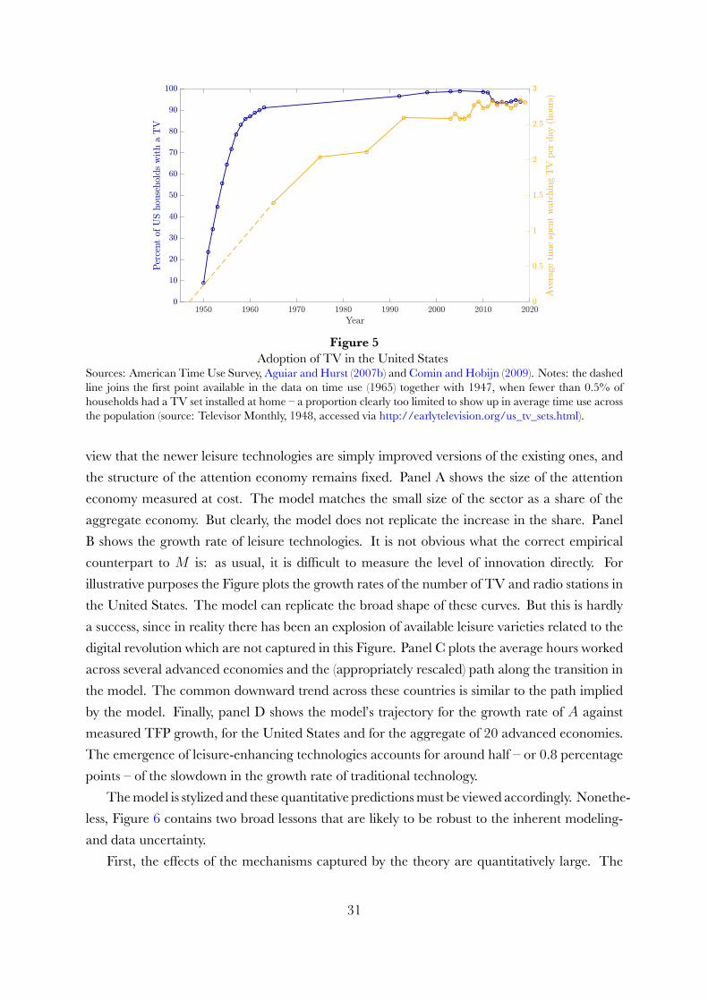
Figure 5Adoption of TV in the United States

Sources: American Time Use Survey, Aguiar and Hurst (2007b) and Comin and Hobijn (2009). Notes: the dashedline joins the first point available in the data on time use (1965) together with 1947, when fewer than 0.5% ofhouseholds had a TV set installed at home – a proportion clearly too limited to show up in average time use acrossthe population (source: Televisor Monthly, 1948, accessed via http://earlytelevision.org/us_tv_sets.html).

view that the newer leisure technologies are simply improved versions of the existing ones, andthe structure of the attention economy remains fixed. Panel A shows the size of the attentioneconomy measured at cost. The model matches the small size of the sector as a share of theaggregate economy. But clearly, the model does not replicate the increase in the share. PanelB shows the growth rate of leisure technologies. It is not obvious what the correct empiricalcounterpart to M is: as usual, it is difficult to measure the level of innovation directly. Forillustrative purposes the Figure plots the growth rates of the number of TV and radio stations inthe United States. The model can replicate the broad shape of these curves. But this is hardlya success, since in reality there has been an explosion of available leisure varieties related to thedigital revolution which are not captured in this Figure. Panel C plots the average hours workedacross several advanced economies and the (appropriately rescaled) path along the transition inthe model. The common downward trend across these countries is similar to the path impliedby the model. Finally, panel D shows the model’s trajectory for the growth rate of A againstmeasured TFP growth, for the United States and for the aggregate of 20 advanced economies.The emergence of leisure-enhancing technologies accounts for around half – or 0.8 percentagepoints – of the slowdown in the growth rate of traditional technology.

Themodel is stylized and these quantitative predictionsmust be viewed accordingly. Nonethe-less, Figure 6 contains two broad lessons that are likely to be robust to the inherent modeling-and data uncertainty.

First, the effects of the mechanisms captured by the theory are quantitatively large. The

31

Figure 6The Model’s Growth Path versus the Trends Observed in the Data

Data sources as in Figure 2, except for the top-right panel in which the data are from the Federal CommunicationsCommission and Statista. These data are interpolated over the missing values. The black lines with empty circlesshow transition following the entry of platforms in 1950. The pink line with filled circles show the transition withadditional shocks to parameters χ (increase) and Ψ (decrease) calibrated in such a way that the size of the leisuresector matches the data in the top-left panel.

simple model, which features only two additional parameters (ν and χ) relative to a standardbenchmark, can potentially account for a significant proportion of the decline in traditionalsector total factor productivity and for most of the cross-country decline in hours worked. Allthis despite the attention economy being minuscule in the aggregate. The lesson here is not todiscount the attention economy as important for macro merely because it is small: the macroe-conomic effects come about not through its size, but indirectly through its influence on the timeallocation decisions of the consumers.

Second, one needs to go beyond the endogenous entry of the leisure sector that I studied sofar to better capture the developments observed in the data. This is not at all surprising: clearly,the attention economy itself has undergone dramatic technological shifts over the decades, someof which go well beyond the steady pace of progress in M captured in the baseline simulation

32

considered so far. For example, panel A of Figure 6 shows that the balanced growth path withconstant preference- and technological parameters is a good description of the first few decadesfollowing the adoption of television, but struggles to account for what happened in the digitalsphere over the past thirty years or so. Put differently, in some ways the leisure technologies wesee today represent a natural progression from those that we saw in the 1950s, but in othersthere are structural differences that, in the context of the model, would show up as changes inmodel’s parameters.

To provide an illustration of such shifts, consider the pink lines with filled circles in Figure 6which show the transitional dynamics if, in addition to the entry of the platforms in 1950, theeconomy experiences a shift in parameters that is sufficient to match the rise in the relative sizeof the attention economy since late 1970s shown in panel A of the Figure. Specifically, I con-sider a steady increase in the perceived effectiveness of brand equity χ and a rise in the degreeof competition among the platforms (a fall in the mark-upΨ),48 starting in the late 1970s. PanelB shows that the expanded production of brand equity can in equilibrium support faster growthof leisure technologies, which leads to a sharper decline in hours worked in the market, shownin panel C. This more rapid decline in hours leads to an additional downward drag on tradi-tional productivity (panel D). The model’s prediction is thus that the rapid leisure-enhancingtechnological change co-exists (and causally leads to) low traditional productivity growth.

Future work could usefully explore ways of capturing some of the structural differences be-tween the leisure technologies of today and those available in the past. These differences includedata gathering, user-generated content, or the portability of devices through which leisure tech-nologies can be accessed.49 Once these shifts are mapped to model parameters, the frameworkcan be used to study the potential effects of these changes for the phenomena observed in thedata. Appendix E provides some further analysis along these lines.

5.4.1 Cross-country evidence on the market-size effect

In light of the theory, the equilibrium level of leisure technologies depends onmarket size. Figure7 provides a simple test of this prediction, by regressing the number of TV channels acrosscountries on GDP per capita, population and the level of aggregate GDP separately in thethree consecutive panels. The number of TV channels is a useful metric ofM in the context ofcross-country analysis, because of the language- and culture- barriers tend to limit the marketto national borders.50 The results suggest that both the level of development and the size of thepopulation matter in determining how many options individuals have when they switch on their

48Which is isomorphic to an increase in platforms’ productivity in turning consumers’ time into brand equity.49This portability enables leisure consumption during all hours of the day, including at work – see Figure A.5 in

Appendix A.50For some other leisure technologies such as mobile phone apps the market is global and cross-country exercise

may be less useful. This concern could also apply to the English-speaking countries in the case of TV though.

33

Figure 7The Number of TV Channels and Market Size

Sources: Data on GDP per capita are from Penn World Tables 9.0 (Feenstra et al. (2015)). Data on population arefrom the World Bank. Data on the number of TV channels in each country has been hand collected from onlinesources. As such these data are subject to some measurement error. TV channels include state-run channels.

TV. In effect, the number of TV channels is best predicted by aggregate GDP (the final panel),with R2 of nearly 70%.

Having discussed the impact of leisure technologies on the attention economy, I now proceedto the analysis of the implications for measurement and welfare.

6 Measuring the leisure economyLeisure technologies and the services that they provide are not captured in headline GDP statis-tics. The 2008 UN System of National Accounts views platforms as advertising agencies: theiroutput is ads, which serve as intermediate inputs of the ad-buyers (Byrne et al. (2016b), (Bean,2016)).51 Two questions arise in this context. First, does this mean that GDP is mismeasured?And second, does the attention economy make GDP a less reliable guide to welfare? In this

51To illustrate this, it is useful to demonstrate measuring GDP using the output-, expenditure- and income ap-proaches in the model economy. The output measure is the sum of value added in the final, intermediate andplatform sectors:

GDP (O) = (Y −Ax) + (Ax−B) +B = Y.

This equation shows explicitly that brand equity output of the platforms is netted out as an intermediate in theproduction of differentiated goods. The expenditure measure is the sum of consumption, investment and capitalconsumption:

GDP (E) = C + K + δK = Y

34

Section I explain why the answers to these questions are ‘no’ and ‘yes’, respectively.52

6.1 Production cost-based value of leisure technologies

To answer the first question it is useful to be precise about what GDP is designed to capture.There is an ongoing debate about this issue: while GDP has been designed as a measure of(market) production, in practice it includes elements that are outside of the production boundary,such as home production of goods, or services from owner-occupied housing, and, for the lackof an agreed more comprehensive measure of economic wellbeing, it is often used as measureof welfare (see Jorgenson (2018) for an overview of the history and the vast literature on theseissues, and Coyle (2017) for an extensive discussion of the production boundary in the context ofdigital goods). Sticking to the use its originators, including Simon Kuznets, intended for GDP,does the attention economy as described in this paper lead to mismeasurement? Since leisuretechnologies are used for consumption by households, they should be included: the view ofthe platforms as solely ad-agencies misses out on their role as leisure-innovators. One strikingexample of this is that if a consumer switches from a paid-for to a zero price product, GDPdeclines. To deal with this issue, Nakamura et al. (2017) propose valuing the production of theseservices at cost, consistent with the usual treatment in the National Accounts. In the context ofthe present model this cost is:

V1 := w · LM =α2χ

Ψ(1− α)Y (50)

where the second equality follows from substituting the equilibrium value of wages. An imme-diate implication of (50) is that V1 grows at the same rate as output.

6.2 Consumption-based measures of value

The production-based measure discussed above does not attempt to capture the consumer sur-plus from free technologies. For that, one must turn to measures on the consumption side. The

where the final equality follows from the resource constraint. Finally, the income measure is the sum of wagepayments, profits, rent payments and households’ outlays on patents:

GDP (I) = ((1− sA − sM )wY + sAwA + sMwM )hN + JΠB +AΠ+ (r + δ)K − V A =

= (1−α)Y +V ·AϕLA +α2χ

Ψ(1− α)Y +

(α2χY − α2χ

Ψ(1− α)Y

)+αY (1− α− αχ)+α2Y −V ·AϕLA =

= Y.

GDP in this economy is simply equal to final output Y . Clearly, GDP does not include leisure technologies.52To meaningfully talk about welfare effects of leisure technologies, in the remainder of the paper I assume that

households’ utility follows (6): that is, more leisure technologies raise utility. Specifically, I use the formulation ofinstantaneous utility that is consistent with balanced growth: u = log c+M

1ν−1 (1− h).

35

literature has considered valuing leisure time at an ongoing wage (Goolsbee and Klenow (2006),Brynjolfsson and Oh (2012)) to capture the surplus. In addition to this measure, the modelcan be deployed to directly compute the compensating variation measure which answers thefollowing question: how much would aggregate consumption had to increase to compensateconsumers for a lack of access to leisure technologies? The two measures are given by:

V2a := N · w ·M

0

ℓ(ι)dι =1− α

1− sA − sM

1− h

hY (51)

V2b := N(c− c) =(exp

((1− h)M

1ν−1

)− 1)C. (52)

where again the second set of equalities follows from substituting in the equilibrium values.

6.3 Analysis

Proposition 7. Measurement of the growth rates. In equilibrium, the production cost-based mea-sure V1 is proportional to output. The value of leisure technologies derived from the consumption side V2a andV2b grow faster than output even in the long-run:

γV1 = γY < γV2

Proof. Appendix B.

The Proposition says that production-cost adjustments will leave growth of the enhancedmeasure of activity unchanged, relative to measured GDP. Conversely, the consumption based-adjustments will alter the growth rate. The underlying reason for why the production- andconsumption-based measures give a different read is strong non-rivalry: in the attention econ-omy, consumption is detached from production.

To illustrate these results quantitatively, Figure 8 plots the level and the growth rate of GDPper capita following the current measurement methodology, together with the ‘enhanced’ GDPmetrics that include the values computed above. The Figure corresponds to the simulationdiscussed in Section 5.

36

Figure 8The Level and the Growth Rate of GDP and the Enhanced Measures of Activity

Because the leisure sector is small in the aggregate, the production cost-based measures donot make much difference to the level of activity. Including consumption-side measures on theother hand makes a significant difference not only to the level but also to the growth rate, in linewith Proposition 7. Quantitatively, the consumption-based measures boost the growth rate by0.4% per annum, which is roughly the negative of the growth rate of the hours worked. Thismagnitude of the quantitative effects is similar to some of the estimates reported in the earlierwork.53

The time-cost approach tracks the path of instantaneous utility of the representative agentclosely, suggesting that it can be a useful measure in practice. Quantitatively, the welfare gainsfrom free technologies can make-up around half of the slowdown in activity.

What with the other half ? Despite accounting for the utility benefits of free leisure, thegrowth rate of utility declines and stays depressed for many decades.54 This may appear sur-prising at first: the time-cost based measure effectively ‘relabels’ leisure time as productive time,it might thus appear that once it is added to GDP, the resulting measure of economic activitywould not deviate from the continuation of its initial trend. The reason why this logic is incor-rect is that it ignores the general equilibrium feedback from hours worked and the growth rate ofTFP. Even as one values hours spent on leisure at the current marginal product of labor, this doesnot recover the lost ground in activity because the marginal product of labor declines relative

53E.g. Brynjolfsson and Oh (2012) find the effect of around 0.3 percentage points per annum.54The effect ultimately turns around, since the consumption utility increases linearly and leisure utility increases

exponentially. But the negative effect dominates for more than 300 years in the simulations.

37

to the no-leisure-economy counterfactual. Furthermore, the negative productivity effect alwaysdominates the positive leisure utility effect for some time after t, since the level of consumptionutility is much higher than the level of leisure utility. To see this, note that in equilibrium, fort ≥ t, utility is:55

u = log(c) + Φ

(1

h− 1

). (53)

Clearly, the second term is small when h is close to 1. And the corollary of Proposition 3 isthat consumption is relatively large when the leisure sector emerges. Together, these implythat the first term on the right hand side of (53) is much larger than the second. So while theconsumers are willingly substituting away from consumption and towards leisure on the margin,the adverse productivity effect lowers the growth rate of consumption, hurting consumers a lotsince consumption is a much larger component of utility in levels.

The productivity effect is clearly external to the individual choices. In the next Section Idiscuss the efficiency aspects of the attention economy.

7 EfficiencyLeisure-enhancing technological change introduces two additional inefficiencies to the marketequilibrium.56 The static inefficiency arises because platforms only benefit from the provision ofMindirectly: the supply of leisure technologies is in equilibrium driven by the price of brand equityrather than themarginal rate of substitution between leisure technologies and consumption. Thedynamic inefficiency results from the adverse effects of leisure today on productivity growth in thefuture. Before discussing those inefficiencies in some detail, I briefly remark on the optimal levelof advertising.

7.1 Brand equity in socially-optimal allocation

Given the combative nature of brand equity competition in the benchmark model, the planneris indifferent as to the level of brand equity as long as its provision requires no extra resources:

Lemma 6. Optimal brand equity. For a given (optimal) choice of leisure hours ℓ∗, the planner isindifferent between producing any amount of brand equity between 0 and B(ℓ∗). If there was an infinitesimalreal resource cost to production of brand equity then the planner would choose to produce none.

Proof. Follows immediately from the fact that for a given level of ℓ∗ the choice ofB∗ in [0, B(ℓ∗)]

has no impact on the resource constraint or utility.

55To see this, use equation (20) in u = log c+M1

ν−1 (1− h).56In addition to the inefficiencies familiar from the literature on optimal growth: the presence of monopolistic

competition, externalities to R&D and possibly duplication externalities in research. For the analysis of theseexternalities see Jones (2015).

38

In what follows I assume that B∗ = 0, but this is clearly without the loss of generality.

7.2 Static inefficiency

Consider a static setup in which an economy is endowed with exogenously given levels of capitalstockK and knowledgeA.57 The supply side is identical to before, except there is no traditionalR&D sector (since A is fixed). In particular, intermediate firms advertise and platforms supplybrand equity and leisure technologies. Households maximize a separable utility function:

U = u(C) + v(1− h,M)

Since there is no saving, market clearing requires C = Y . Equilibrium conditions naturallymirror those in the dynamic model and I compare them to the social optimality conditionsmomentarily.

I study the following unconstrained problem of the social planner:

maxh,sM

u(C) + v(1− h,M) s.t. Y = FY (K,A, h, sM), M = FM(A, h, sM) and Y = C. (54)

The planner maximizes social welfare subject to technology and resource constraints. (54) isan unconstrained problem in the sense that the planner has control over time allocation of therepresentative household: h is one of the two choice variables. Another is the share of laboremployed in theM sector. These two controls determine traditional output and consumption,as well as the level of leisure technologies.

Socially optimal h∗ satisfies the necessary condition

∂u(C)

∂C

∂Y

∂h+∂v(1− h,M)

∂M

∂M

∂h≥ ∂v(1− h,M)

∂h(55)

which holds with equality if h∗ is interior. This condition compares the utility benefit of addi-tional time spent working – higher consumption and more leisure technologies – with the cost:the loss of leisure utility as a result of working more. The equivalent condition in the decentral-ized equilibrium is:58

∂u(C)

∂C

∂Y

∂h+∂u(C)

∂C

pBΨ

1− h

M

∂M

∂h≥ ∂v(1− h,M)

∂h. (56)

The difference between the two conditions lies in the way M is valued. In condition (55) this57I assume that the level of capital is such that the capital-to-output ratio at full employment is constant and

equal to 3 – that is, I consider pairs of A and K such that capital varies linearly with A: K = 31

1−αA.58To see this, note that households’ labor income is (wY (1− sM ) + wMsM )h. Wages in the two sectors are

wY = ∂Y∂LY

= ∂Y∂h

11−sM

and wM = pB · 1Ψ · 1−h

M · ∂M∂LM

= pB · 1Ψ · 1−h

M · ∂M∂h

1sM

. Combining these expressionswith the optimality condition ∂u

∂C (wY (1− sM ) + wMsM ) ≥ ∂v∂h yields (56).

39

value is ∂v(1−h,M)∂M

: the utility that this technology brings to the consumer on the margin. Butin condition (56) it is the marginal revenue product of a platform, and that revenue comes fromthe sales of brand equity, not leisure technology. Put differently, the wage in the leisure sectordoes not reflect the marginal revenue product of the free technologies – instead, it reflects themarginal revenue product of brand equity. Since workers choose their labor supply based on theongoing wage, the distortion in the level of wages translates into the distortion in hours worked.

The same distortion also affects the allocation of labor across sectors. The optimal share oflabor employed in the platform sector satisfies

− ∂Y

∂sM≥ ∂M

∂sM

∂v/∂M

∂u/∂C︸ ︷︷ ︸MRSM,C

. (57)

Condition (57) compares the marginal cost and the marginal benefit of shifting labor away fromproduction of the consumption good and towards the platform sector. The corresponding con-dition in equilibrium is:59

− ∂Y

∂sM≥ ∂M

∂sM

1− h

M

pB︸︷︷︸wrong price

+∂pB∂Bj︸︷︷︸

market power

. (58)

Comparing conditions (57) and (58) we see that the exact same distortion drives misallocation.In addition, the allocation of labor across industries is distorted due to the market power ofplatforms: since the term ∂pB

∂Bjis non-positive, market power has the usual effect of making the

sector too small relative to the optimum. But the market power distortion is insignificant relativeto the distortion that stems from the platforms’ business model.

To illustrate what this inefficiency means for the calibrated model, Figure 9 compares theoptimal and equilibrium allocations for different levels of A (and implicitly K ). Clearly, in astatic economy calibrated with parameter values in Table 1 the optimal allocation features amuch higher share of labor devoted to leisure innovation, compared to the equilibrium. Thisdistortion affects both the point at which leisure technologies become available (the plannerchooses positiveM at comparatively much lower levels ofA) and the extent, or intensive margin,of the provision of leisure technologies.

59This follows from differentiating ∂∂sM

(pB ·Bj).

40

Figure 9Socially optimal allocation and equilibrium in the static model

Note: The Figure plots the socially optimal allocation and equilibrium allocation for different values of A andimplicitlyK, holding the capital-to-output ratio constant at 3.

7.3 Dynamic inefficiency

The dynamic inefficiency arises because leisure technologies translate into lower future produc-tivity – an effect that is external to the individual choices. Consider the planner’s constraineddynamic optimization problem. When maximizing social welfare, the planner must respecthouseholds’ time allocation decisions

h = min1,ΦM1

1−ν where Φ =

(1− α

1− s− sM

Y

C

) θθ+1

.

This implies that h is a function of sM (since h depends onM ). The Hamiltonian of this problemis:

H(K,A,C, s, sM ;µK , µA) = u(c) + v(1− h,M) + µK(Y − C − δK) + µAA,

where µK and µA are the costate variables associated with capital and the level of traditionaltechnology. The relevant necessary condition is:

∂v

∂h

∂h

∂sM+

∂v

∂M

(∂M

∂sM+∂M

∂h

∂h

∂sM

)︸ ︷︷ ︸

utility benefit

+ µK

(∂Y

∂sM+∂Y

∂h

∂h

∂sM

)︸ ︷︷ ︸

static output cost

+ µA

(∂A

∂h

∂h

∂sM

)︸ ︷︷ ︸

dynamic TFP cost

= 0.

The final term reflects the dynamic cost that is absent from the decentralized problem.I collect the efficiency results in the following proposition.60

60The dynamic externality highlighted here is a separate issue to the externality that has been at the center of theliterature on endogenous growth: the positive externalities to R&D. Specifically, the dynamic inefficiency wouldstill be present with an R&D subsidy that internalizes the learning externalities from product innovation. The two

41

Proposition 8. Efficiency of market equilibrium. Platform’s ad-based business model results ina static inefficiency since the wrong price values leisure technologies in equilibrium. This distortion suggests thatthere is insufficient supply of leisure technologies in equilibrium. There is also a dynamic inefficiency as more timespent on leisure lowers future productivity. This inefficiency means the supply of leisure technologies in equilibriumis too high.

8 ConclusionIn this paper I formalized the idea of leisure-enhancing technologies: products that are availablefor free and are thus specifically designed to capture our time and attention. Using the theoryI studied how these technologies shape the growth patterns and what the welfare consequencesare. The main takeaway is that these endogenously time-biased technologies can simultaneouslyexplain shifts in hours worked and account for the low growth observed in the data. The effecton GDP growth reflects both the measurement difficulties and the ‘real’ slowdown, since leisuretechnologies fail to fully compensate for the crowding out of traditional productivity.

The analysis can be extended in many interesting directions. To organize thoughts, thisconcluding Section presents an account of how one might interpret developments in leisureeconomy over the past century through the lens of the model. Such historical narrative is nec-essarily more speculative than the analysis thus far, but it is interesting, and it helps spot gapsand spur ideas.

The theory delivered the conclusion that the size of the economy determines whether leisuretechnologies are viable or not. But other factors play a role too.

One such factor is the share of time that households can feasibly allocate to marketableleisure. The first half of the 20th century saw a substantial increase in this share. Two historicalevents were key: the introduction of the two-day weekend in the 1930s61 and the gradual adop-tion of household appliances – the washing machine, the flush toilet, the vacuum and others– from 1920s through 1940s and beyond. Both of these freed up time for other activities.62 Itis plausible that these developments have acted to direct resources towards inventions and ac-tivities that complement leisure and leisure time, in the spirit of the directed technical changeliterature (Acemoglu, 2002). Incorporating these mechanisms in the model and assessing theirempirical validity is an interesting avenue for future work.

Second, the audio-visual entertainment revolution that started in the 1920s and rapidly ac-celerated in the 1950s has been propelled by the introduction of general purpose technologies

externalities may interact in interesting ways, and the optimal R&D subsidy policy in the context of both is aninteresting area for future work.

61In the US, Henry Ford made Saturday and Sunday days off for his staff as early as 1926, and the US as a wholeadopted the five-day system in 1932 (in part to counter the unemployment caused by the Great Depression).

62This is especially interesting since the model presented here abstracted from home production – a margin thatis clearly important in practice.

42

that allowed for the signal to be transmitted to households: the radio receiver and the televi-sion set. More recently, invention of PCs, smartphones and tablets made it possible for the freeleisure technologies to spread far and wide (Figure 10).

Figure 10Adoption of leisure-linked general purpose technologies

Sources: Comin and Hobijn (2009).

To analyze these one could bring in the insights from Fernald and Jones (2014) on model-ing general purpose technologies into the framework developed here. An alternative that stayscloser to the current model is to view the arrival of these technologies as exogenous shifts inthe productivity parameters of the leisure technology production functions: each of these GPTsmade the delivery of free leisure services easier and cheaper and boosted the ability of plat-forms to turn consumers’ time and attention into brand equity.63 Appendix E presents analysisalong those lines. It shows that such changes effectively turbo-charge the development of leisuretechnologies, exacerbating the effects discussed in the main body of the paper and potentiallyexplaining the rise of large and highly profitable platforms.

Relatedly, the arrival of the internet, social media and smartphones has arguably been associ-ated with a culture shift towards online activities among consumers. One particularly intriguingfeature is the ubiquity of user-generated content: for example, social media are largely popu-

63Another effect of the GPTs such as computers and smartphones is that they blur the boundary between leisureand work, enabling leisure consumption at the workplace and making it easier for workers to engage in productiveactivities at home. Eldridge and Pabilonia (2010) study how ‘bringing work home’ affects the level and the growthrate of hours worked. They identify 0.7-0.9% downward bias in the level of hours worked due to prevalence ofunpaid work at home in the period 2003-08, much of which has been enabled by the technologies mentionedabove. However, they find no evidence that the growth rate over the period 2003-08 is affected, and consequentlyconclude that unpaid work from home over that period did not alter the observed trend in productivity growth. Ina recent contribution, Restrepo and Zeballos (2020) study workers who work from home regularly (one day a weekfor example), and find that working from home cuts the time spent on grooming and commuting and leaves moretime for food preparation and for leisure.

43

lated by content created by consumers, whereby a platform is just that: a platform that connectspeople and facilitates content generation.

An open question is how the rise of the leisure sector interacts with heterogeneity, both at thehousehold and at the firm level. On the household side, it is interesting to study how time alloca-tion decisions interact with income and wealth inequality. For example, disaggregated evidenceon time allocation across the income distribution shows that poor individuals increased theirleisure more than the rich (Boppart and Ngai, 2017b). Allowing for household and income het-erogeneity in the presence of leisure-enhancing technologies could bring out new insights and aidthe debate on leisure-inequality and the welfare implications. Considering firm heterogeneitymay be important, too: the current setting is well suited to analyze equilibrium outcomes whenheterogenous firms compete not only in prices but also in intangible assets. More productivefirms may devote more resources to brand building, cementing their market share, with inter-esting implications for market power (De Loecker and Eeckhout, 2017). To tackle these issues,the framework developed here could be usefully incorporated into a model of firm dynamicsand growth in the tradition of Klette and Kortum (2004).

As leisure economy becomes ever more important going forward, the framework built herecan be used as a base for explorations of some of the pressing policy questions, such as optimaltaxation of platforms or competition- and anti-trust policy in presence of zero-price services.These ideas formulate an exciting research agenda for economics in general, and macroeco-nomics specifically, in the years to come.

44

ReferencesAcemoglu, D. (2002). Directed Technical Change. Review of Economic Studies, 69 (4), 781–809.— and Guerrieri, V. (2008). Capital Deepening and Nonbalanced Economic Growth. Journal of Political

Economy, 116 (3), 467–498.Adler, G., Duval, R., Furceri, D., Kiliç Çelik, S., Koloskova, K. and Poplawski-Ribeiro, M. (2017). Gone

with the Headwinds: Global Productivity. IMF Staff Discussion Notes, 17 (04), 1.Aghion, P., Akcigit, U. and Howitt, P. (2014). What DoWe Learn From Schumpeterian Growth Theory?

Handbook of Economic Growth, 2, 515–563.— and Howitt, P. (1992). A Model of Growth Through Creative Destruction. Econometrica, 60 (2), 323–

351.—, Jones, B. and Jones, C. (2017). Artificial Intelligence and Economic Growth.Aguiar, M., Bils, M., Charles, K. K. and Hurst, E. (2017). Leisure Luxuries and the Labor Supply of Young Men.

Tech. rep., National Bureau of Economic Research, Cambridge, MA.— and Hurst, E. (2007a). Measuring Trends in Leisure: The Allocation of Time Over Five Decades. The

Quarterly Journal of Economics, 122 (3), 969–1006.— and — (2007b). Measuring trends in leisure: the allocation of time over five decades. The Quarterly

Journal of Economics, 122 (3), 969–1006.— and — (2008). The Increase in Leisure Inequality. Tech. rep., National Bureau of Economic Research,

Cambridge, MA.— and — (2016). The Macroeconomics of Time Allocation. In Handbook of Macroeconomics, vol. 2, pp.

1–44.—, — and Karabarbounis, L. (2012). Recent developments in the economics of time use. Annual Review

of Economics, 4, 373–397.Akcigit, U. and Kerr, W. R. (2018). Growth through heterogeneous innovations. Journal of Political Economy,

126 (4).Anderson, S. P. and Renault, R. (2006). Advertising Content. American Economic Review, 96 (1), 93–113.Armstrong, M. (2006). Competition in two-sided markets. RAND Journal of Economics, 00 (3), 668–691.Bagwell, K. (2007). Chapter 28 The Economic Analysis of Advertising. In Handbook of Industrial Organisa-

tion, pp. 1701–1844.Basu, S., Fernald, J. G. andKimball, M. S. (2006). Are technology improvements contractionary? American

Economic Review, 96 (5), 1418–1448.Bean, C. (2016). Independent Review of UK Economic Statistics. Tech. rep.Becker, G. S. (1965). A Theory of the Allocation of Time. The Economic Journal, 75 (299), 493–517.— and Murphy, K. M. (1993). A Simple Theory of Advertising as a Good or Bad. The Quarterly Journal of

Economics, 108 (4), 941–964.Benhabib, J. and Bisin, A. (2002). Advertising, Mass Consumption and Capitalism. Working Paper, pp.

1–38.Bloom, N., Jones, C., Van Reenen, J. and Webb, M. (2017). Are Ideas Getting Harder to Find? Tech. rep.,

National Bureau of Economic Research, Cambridge, MA.—, Jones, C. I., van Reenen, J. and Webb, M. (2020). Are ideas getting harder to find? American Economic

Review, 110 (4), 1104–1144.Boppart, T. and Krusell, P. (2020). Labor Supply in the Past, Present, and Future: A Balanced-Growth

Perspective. Journal of Political Economy, 128 (1), 118–157.— and Ngai, L. (2017a). Rising inequality and trends in leisure. (DP12325).— and Ngai, L. R. (2017b). Rising inequality and trends in leisure.Borden, N. H. (1942). Findings of the Harvard Study on the Economic Effects of Advertising. Journal of

Marketing, 6 (4), 89–99.

45

Bridgman, B. (2018). Is Productivity on Vacation? The Impact of the Digital Economy on the Value ofLeisure.

Broda, C. and Weinstein, D. E. (2006). Globalization and the Gains From Variety. The Quarterly Journal ofEconomics, 121 (2), 541–585.

Brynjolfsson, E., Eggers, F. and Gannamaneni, A. (2018). Using Massive Online Choice Experiments to MeasureChanges in Well-being. Tech. rep., National Bureau of Economic Research, Cambridge, MA.

— and Oh, J. H. (2012). The attention economy: Measuring the value of free digital services on theinternet. International Conference on Information Systems, ICIS 2012, 4, 3243–3261.

Butters, G. R. (1977). Equilibrium Distributions of Sales and Advertising Prices. The Review of EconomicStudies, 44 (3), 465.

Byrne, D. M., Fernald, J. G. and Reinsdorf, M. B. (2016a). Does the United States have a productivityslowdown or a measurement problem? Brookings Papers on Economic Activity.

—, — and — (2016b). Does the united states have a productivity slowdown or a measurement problem?Brookings Papers on Economic Activity, 2016 (SPRING), 109–182.

Cavenaile, L. and Roldan-Blanco, P. (2020). Advertising, Innovation and Economic Growth.Chamberlin, E. (1933). The theory of monopolistic competition. Harvard University Press.Christensen, M. A., Bettencourt, L., Kaye, L., Moturu, S. T., Nguyen, K. T., Olgin, J. E., Pletcher, M. J.

and Marcus, G. M. (2016). Direct Measurements of Smartphone Screen-Time: Relationships withDemographics and Sleep. PLOS ONE, 11 (11).

Comin, D. A. and Hobijn, B. (2009). The CHAT Dataset. Tech. rep.Corrado, C., Haskel, J., Jona-Lasinio, C. and Iommi, M. (2012). Intangible Capital and Growth in Ad-

vanced Economies: Measurement Methods and Comparative Results.Corrado, C. A. and Hulten, C. R. (2010). How Do You Measure a Technological Revolution? American

Economic Review, 100 (2), 99–104.Coyle, D. (2017). Do-it-yourself digital: the production boundary, the productivity puzzle and economic

welfare Diane Coyle Professor of Economics, University of Manchester, and ONS Fellow 1. pp. 1–38.De Loecker, J. and Eeckhout, J. (2017). The Rise of Market Power and the Macroeconomic Implications. Tech.

rep., National Bureau of Economic Research, Cambridge, MA.DellaVigna, S. and Gentzkow, M. (2010). Persuasion: Empirical Evidence. Annual Review of Economics,

2 (1), 643–669.Dixit, A. and Norman, V. (1978). Advertising and Welfare. The Bell Journal of Economics, 9 (1), 1.Dixit, A. K. and Stiglitz, J. E. (1977).Monopolistic Competition andOptimumProduct Diversity. American

Economic Review, 67 (3), 297–308.Dorfman, R. and Steiner, P. O. (1954). Optimal Advertising and Optimal Quality. The American Economic

Review, 44 (5), 826–836.Eldridge, L. P. and Pabilonia, S. W. (2010). Bringing work home: Implications for BLS productivity

measures. Monthly Labor Review, 133 (12), 18–35.Falck, O., Gold, R. andHeblich, S. (2014). E-lections: Voting behavior and the internet. American Economic

Review, 104 (7), 2238–2265.Farboodi, M. and Veldkamp, L. (2019). A Growth Model of the Data Economy.Feenstra, R. C., Inklaar, R., Timmer, M. P., Aten, B., Atkeson, A., Basu, S., Deaton, A., Diewert, E.,

Heston, A., Jones, C., Rao, P., Rodríguez-Clare, A. and Végh, C. (2015). The Next Generation of thePenn World Table. American Economic Review, 105 (10), 3150–3182.

Fernald, J. G. and Jones, C. I. (2014). The future of US economic growth. American Economic Review, 104 (5),44–49.

Gentzkow, M. (2006). Television and Voter Turnout*. Quarterly Journal of Economics, 121 (3), 931–972.— and Shapiro, J. M. (2008). Preschool Television Viewing and Adolescent Test Scores: Historical Evi-

dence from the Coleman Study. Quarterly Journal of Economics, 123 (1), 279–323.

46

Goolsbee, A. and Klenow, P. J. (2006). Valuing consumer products by the time spent using them: Anapplication to the Internet. In American Economic Review, vol. 96, pp. 108–113.

Gourio, F. and Rudanko, L. (2014). Customer capital. Review of Economic Studies, 81 (3), 1102–1136.Grossman, G. M. and Shapiro, C. (1984). Informative Advertising with Differentiated Products. The

Review of Economic Studies, 51 (1), 63.Hall, R. E. (2008). General equilibrium with customer relationships: a dynamic analysis of rent-seeking.

Working Paper, pp. 1–35.Hulten, C. and Nakamura, L. (2017). Accounting for Growth in the Age of the Internet: The Importance

of Output-Saving Technical Change.Working Paper, pp. 1–36.Johnson, J. P. (2013). Targeted advertising and advertising avoidance. RAND Journal of Economics, 44 (1),

128–144.Jones, C. I. (1995). R&D-BasedModels of Economic Growth. Journal of Political Economy, 103 (4), 759–784.— (2015). The Facts of Economic Growth. The Handbook of Macroeconomics Volume 2, pp. 0–81.— and Tonetti, C. (2019). Nonrivalry and the economics of data.Jorgenson, D. W. (2005). Chapter 10 Accounting for Growth in the Information Age.Handbook of Economic

Growth, 1 (SUPPL. PART A), 743–815.— (2018). Production andwelfare: Progress in economicmeasurement. Journal of Economic Literature, 56 (3),

867–919.Kelly, Y., Zilanawala, A., Booker, C. and Sacker, A. (2018). Social Media Use and Adolescent Mental

Health: Findings From the UK Millennium Cohort Study. EClinicalMedicine, 6, 59–68.King, R. G., Plosser, C. I. and Rebelo, S. T. (1988). Production, growth and business cycles. Journal of

Monetary Economics, 21 (2-3), 195–232.Klein, E. (2016). Technology is changing how we live, but it needs to change how we work.Klette, T. J. and Kortum, S. (2004). Innovating Firms and Aggregate Innovation. Journal of Political Econ-

omy, 112 (5).Kortum, S. (1997). Research, Patenting, and Technological Change. Econometrica, 65 (6), 1389–1419.Lambin, J. J. (1976). Advertising, Competition and Market Conduct in Oligopoly Over Time. Amsterdam: North-

Holland.Lewis, R. A. and Rao, J. M. (2015). The unfavorable economics of measuring the returns to advertising.

Quarterly Journal of Economics, 130 (4), 1941–1973.— and Reiley, D. H. (2014). Online ads and offline sales: Measuring the effect of retail advertising via a

controlled experiment on Yahoo! Quantitative Marketing and Economics, 12 (3), 235–266.Marshall, A. (1890). Principles of Economics. London: MacMillan and Co. Ltd, 8th edn.Michel, C., Sovinsky, M., Proto, E. and Oswald, A. J. (2019). Advertising as a major source of human

dissatisfaction: Cross-national evidence on one million europeans. The Economics of Happiness: How theEasterlin Paradox Transformed Our Understanding of Well-Being and Progress, i (November), 217–239.

Milgrom, P. and Roberts, J. (1986). Price and Advertising Signals of Product Quality. Journal of PoliticalEconomy, 94 (4), 796–821.

Molinari, B. and Turino, F. (2009). Advertising and Business Cycle Fluctuations.Nakamura, L., Samuels, J. and Soloveichik, R. (2017). Measuring the ”Free” Digital Economy within the

GDP and Productivity Accounts.Nelson, P. (1974). Advertising as Information. Journal of Political Economy, 82 (4), 729–754.Ngai, L. R. and Pissarides, C. A. (2008). Trends in hours and economic growth. Review of Economic Dy-

namics, 11 (2), 239–256.Nixon, D. (2017). Is the economy suffering from the crisis of attention?Nordhaus, W. D. and Tobin, J. (1972). Is Growth Obsolete?, vol. 5.OECD (2009). Special Focus: Measuring Leisure in OECD Countries. Tech. rep.OfCOM (2019). Online Nation 2019 Report. Tech. Rep. May.

47

Rachel, L. (2020). Leisure-enhancing technologies and structural change.Ramey, V. A. and Francis, N. (2009). A century of work and leisure. American Economic Journal: Macroeco-

nomics, 1 (2), 189–224.Rauch, F. (2013). Advertising expenditure and consumer prices. International Journal of Industrial Organiza-

tion, 31 (4), 331–341.Reis, F. (2015). Patterns of Substitution between Internet and Television in the Era of Media Streaming-

Evidence from a Randomized Experiment.Restrepo, B. J. and Zeballos, E. (2020). The effect of working from home on major time allocations with

a focus on food-related activities. Review of Economics of the Household.Rochet, J.-C. and Tirole, J. (2003). Platform Competition in two-sided markets. Journal of the european

economic association 1 (4), 990-1029.Romer, P. M. (1990). Endogenous Technological Change. Journal of Political Economy, 98 (5), S71–S102.Royal Society for Public Health (2017). Social media and young people’ s mental health and wellbeing.

Royal Society for Public Health,, (May), 32.Scanlon, P. (2018). Why Do People Work So Hard? 2018 Meeting Papers 1206, Society for Economic Dy-

namics.Segerstrom, P. S. (1998). Endogenous Growth without Scale Effects. American Economic Review, 88 (5),

1290–1310.Solow, R. M. (1987). We’d Better Watch out...Stahl, D. O. (1989). Oligopolistic Pricing with Sequential Consumer Search.The American Economic Review,

79 (4), 700–712.Stiglitz, J. E., Sen, A. and Fitoussi, J.-P. (2009). Report by the Commission on the Measurement of Economic Perfor-

mance and Social Progress. Tech. rep.Syverson, C. (2017). Challenges to Mismeasurement Explanations for the US Productivity Slowdown.

Journal of Economic Perspectives, 31 (2), 165–186.Trimborn, T., Koch, K. J. and Steger, T. M. (2008). Multidimensional transitional dynamics: A simple

numerical procedure.Macroeconomic Dynamics, 12 (3), 301–319.Tucker, C. E. (2012). The economics of advertising and privacy. International Journal of Industrial Organization,

30 (3), 326–329.Vandenbroucke, G. (2009). Trends in hours: The U.S. from 1900 to 1950. Journal of Economic Dynamics and

Control, 33 (1), 237–249.Veblen, T. (1899). The Theory of the Leisure Class. MacMillan and Co. Ltd.Wallsten, S. (2013). What Are We Not Doing When We’re Online. Tech. rep., National Bureau of Economic

Research, Cambridge, MA.Ward, A. F., Duke, K., Gneezy, A. and Bos, M. W. (2017). Brain Drain: The Mere Presence of One’s

Own Smartphone Reduces Available Cognitive Capacity. Journal of the Association for Consumer Research,2 (2), 140–154.

48

AppendicesA Illustrative evidenceThis Appendix furthermotivates the focus of this paper and forms a background to the analysis.

Evidence on leisure-enhancing innovations

Figure 2 in the main text illustrated the increased importance of the digital sub-sector of theattention economy since the mid-1990s. The available industry statistics reinforce this message.For example, Figure A.1 shows the dramatic rise in the number of smartphone apps, with themajority available free of charge to the consumer. The fact that millions of apps have beencreated over the past decade is a testament to the innovative efforts of firms in the attentioneconomy.64

Figure A.1Smartphone Apps

Source: The number of apps in Google Play Store is from Google, App Annie and AppBrain. The paid vs freeapps breakdown is from 42matters, an app analytics company.

Consistent with the rapid technological progress within it, the leisure sector appears to bean increasingly important driver of the overall R&D spending. No exact measure for the shareof attention economy in overall R&D spending is available; but it is possible to construct roughproxies by considering a subset of industries which are most likely engaged in leisure-enhancing

64The market structure in the app market is more complex than in the model presented in the main text. Appsare available on platforms such as Google Play Store or Apple App Store, but are produced by many firms, notjust Google or Apple. This additional layer of intermediation does not change the economics of the paper though:the incentives to capture the time and attention of the end-user remains unchanged. Future work could usefullyexplore the competition, business stealing and firm dynamics aspects of the app producers or other firms withinthe broadly defined leisure sector.

49

Figure A.2R&D Expenditure Share of the (Proxy for the) Leisure Economy

Source: OECD. Includes data for an unbalanced panel of 39 countries. The figure shows the median and the in-terquartile range of the country-level share of R&D spending in the following sectors: publishing; motion picture,video and television program production; sound recording; programming and broadcasting activities; telecommu-nications services; computer programming, consultancy and related activities; information service activities; dataprocessing, hosting and related activities; and web portals.

innovations. Figure A.2 shows that the share of R&D spending accounted for by the sectorssuch as video and TV program production, sound recording, broadcasting and web portals hasbeen rising over time.

Recent changes in time allocation patterns

While hours worked in the United States have fallen by less than in other countries (recall themiddle panel of Figure 2), the trend in leisure time has been clearly upwards. Data from theannual American Time Use Survey, available from 2003, show that the largest increase in anycategory has been recorded in the “relaxing and leisure” category. Significantly, the breakdownof the increase reveals that this rise is more-than-accounted-for by changes in the categories mostdirectly related to leisure technologies, such as watching TV or using a computer (Figure A.3).

Nonetheless, there are reasons why the time use survey data may underestimate the time thatactually spent on modern leisure technologies, and perhaps overestimate the time spent working(or at least working attentively). First, the survey aims to uncover a person’s main activity at anygiven point in time during a day, and so if some of the leisure technologies are used during otheractivities (for example during work hours), their use will not be recorded. This is important sincethe evidence (which I discuss below) suggests that smartphones in particular are being used witha constant frequency throughout the day, including during work hours, and some of that useis likely to be related to leisure. For the same reason the BLS acknowledges that ATUS is nota good source of information on time spent online and/or using a computer or a smartphone:the survey is designed in such a way that time is split across the many traditional categories

50

Figure A.3Decomposition of the Increase in Relaxing and Leisure – the Category in the American Time Use

Survey that has Experienced the Largest Increase Since 2003

Source: American Time Use Survey.

such as working, socializing, etc.65 This could give a misleading steer on the use of the leisuretechnologies if, for example, socializing today is different to socializing in the past (in particularif socializing today involved the use of leisure technologies). A related point is that, since peopletend to check their phone very frequently (numerous estimates available online suggest that wepick-up our phones between 50 and 100 times a day), it is likely that the responders under-report usage when they fill in the survey. Consistent with that, some anecdotal evidence andthe popularity screen-time-tracking software suggests that users may find it hard to control thefrequency of use and overall amount of time they spend on their devices. That could suggestpossible underreporting in the surveys.

Given these possible shortcomings of the time-use survey data, the device-tracking data fromNielsen offers useful cross-check (even as it is not without drawbacks). The data paints a pictureof a much more dramatic changes in time-use linked to technology (Figure A.4). For example,the data suggest that the amount of time spent on a smartphone more than quadrupled over thelast 7 years, reaching over 3 hours daily. One of the limitations of these data is that they arenot additive: a person can engage in multiple activities at once (e.g. watching TV and engagingon social media on the smartphone). Another is that the time spent on the devices could beproductive time. Nonetheless, these data are a useful complement to the traditional time usesurveys which naturally struggle to capture the short-but-frequent spells of usage.

The evidence on how people spend time at work (and indeed how much work is being car-ried out at home) is imperfect. For that reason it is useful to consider experimental trackingdata on the frequency of use throughout the day. In one particularly prescient study, Chris-tensen et al. (2016) measured smartphone screen time over the course of an average day among

65See https://www.bls.gov/tus/atusfaqs.htm#24 for the discussion of this point.

51

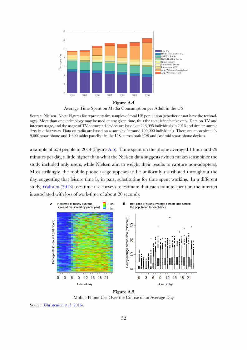
Figure A.4Average Time Spent on Media Consumption per Adult in the US

Source: Nielsen. Note: Figures for representative samples of total US population (whether or not have the technol-ogy). More than one technology may be used at any given time, thus the total is indicative only. Data on TV andinternet usage, and the usage of TV-connected devices are based on 248,095 individuals in 2016 and similar samplesizes in other years. Data on radio are based on a sample of around 400,000 individuals. There are approximately9,000 smartphone and 1,300 tablet panelists in the U.S. across both iOS and Android smartphone devices.

a sample of 653 people in 2014 (Figure A.5). Time spent on the phone averaged 1 hour and 29minutes per day, a little higher than what the Nielsen data suggests (which makes sense since thestudy included only users, while Nielsen aim to weight their results to capture non-adopters).Most strikingly, the mobile phone usage appears to be uniformly distributed throughout theday, suggesting that leisure time is, in part, substituting for time spent working. In a differentstudy, Wallsten (2013) uses time use surveys to estimate that each minute spent on the internetis associated with loss of work-time of about 20 seconds.

Figure A.5Mobile Phone Use Over the Course of an Average Day

Source: Christensen et al. (2016).

52

Indeed, one feature of the latest technology is that it allowed leisure to “compete” with workmuch more directly than has been the case in the past. While it may not have been possibleto watch TV at work, online entertainment is available during the work hours. This is, at leastin part, balanced by the possibility of accessing work emails at home (see Footnote 63). Futureresearch should consider ways of measuring in more detail how people spend time at work andhow much work is done at home.

53

B Proofs

Proof of Lemma 1

Proof. The total amount of marketable leisure time is defined as ℓ :=´M0ℓιdι. By the symmetry

of household’s problem, it is immediate that the optimal choice is to spread free time evenlyacross theM available leisure options and therefore ℓ = Mℓι which implies ℓι = ℓ

M. Plugging

this back into (10) yields the result.

Proof of Lemma 2

Proof. The Hamiltonian associated with household problem (12) is:

H(K,C, h;µK) = log(C/N)−

(hM

1ν−1

)1+ 1

θ

1 + 1θ

+µK

(whN + rK − C − V A+ AΠ+ JΠB

).

The necessary conditions for an interior optimum are:

C−1 = µK (59)(hM

1ν−1

) 1θM

1ν−1 = µKwN (60)

ρµK − µK = µKr. (61)

together with the transversality and the no-Ponzi game conditions:

limt→∞

e−ρtµKK = 0.

Combining these conditions with equation (65) derived below yields:

hθ+1θ M

1ν−1

θ+1θ =

(1− α)Y

(1− sA − sM)C

where sA := LA

LY +LA+LMand sM := LM

LY +LA+LMare the shares of labor employed in the two

R&D sectors. Letting Φ :=(

1−α1−sA−sM

YC

) θθ+1

, we obtain the interior solution:

h = ΦM1

1−ν .

Since hours worked are bounded from above by 1, the solution is:

h = min1,ΦM1

1−ν (62)

54

and since ℓ = 1− h:ℓ = max0, 1− ΦM

11−ν (63)

Proof of Lemma 3

Proof. Suppose that the platform sector is active: Ω = 1. The maximization problem of the finalgood producer is:

maxxi,LY

A

0

((bib

)χxi

)αL1−αY di−

A

0

xiqidi− wLY (64)

The first order conditions are:

(1− α)Y

LY= w (65)

α

(bib

)αχxα−1i L1−α

Y = pi (66)

where pi is the price of variety i of the intermediate good. In a symmetric equilibrium xi = x∀i,ki = k∀i and pi = p∀i. Furthermore, since the linear production technology implies thateach intermediate’s capital is equal to its output, we can define the aggregate capital stock asK := Ax. The final output can be written as

Y =

(b

b

)αχKα ((1− sA − sM)hNA)1−α . (67)

Condition (66) can then be re-written as:

αY

K= p. (68)

The problem of each intermediate producer is (dropping the i subscript):

maxx,b

px− (r + δ)x− pBb (69)

subject to (66) and technology x = k. The first order conditions are:

αp = r + δ (70)

pB = α2χbαχ−1

bαχxαL1−α

Y (71)

55

Together with equation (68), the first of these conditions gives the familiar capital demand con-dition:

α2 Y

K= r + δ. (72)

The optimal output of each producer can be derived from plugging the first order condition intothe demand curve:

x =

(α2

r + δ

(b

b

)αχ) 11−α

LY (73)

which gives the following expression for capital stock:

K = Ax =

(α2

r + δ

) 11−α

ALY . (74)

Equations (73), (71) and (74) yield:

pB = α2χY

A

1

b

(b

b

) α1−α

χ−1

. (75)

In equilibrium bi = b and the results in the Lemma follow immediately from (68), (73) and(75). Equation (75) also implies

pBb = α2χY

A. (76)

Equilibrium profits of intermediate firms are thus:

Π = αY

A(1− α− αχ) . (77)

Proof of Lemma 4

Proof. The optimality condition to problem (26) is:

pB −(1− α

1− αχ

)pB

Ab

Bj +∑

k =j Bk

Bj

Ab= MB.

In a symmetric equilibrium Bj = Bk∀j, k hence:

pB

(1−

(1− α

1− αχ

)1

J

)= MB.

56

Proof of Lemma 5

Proof. In equilibrium price equals markup over marginal cost:

pB = ΨwM

ℓAϕ. (78)

Using (22) we get:

α2χY

B= Ψw

M

ℓAϕ(79)

Since B = ℓ by the platforms’ technology and w = (1− α) Y(1−sA−sM )Nh

we have:

M =α2χ

(1− α)Ψ(1− sA − sM)︸ ︷︷ ︸Υ:=

hNAϕ. (80)

Proof of Proposition 3

Proof. Suppose that ℓ > 0. Combining (62) and (80) and solving forM :

M =(ΥΦNAϕ

) ν−1ν . (81)

Note that under Assumption 3, A = A0en

1−ϕt = A0

(NN0

) 11−ϕ . Equation (63) implies that ℓ > 0

if and only ifM > Φν−1or equivalently that

ΥΦN2−ϕ1−ϕ

A0

N1

1−ϕ

0

ϕ

1ν

> Φ.

So there is leisure-enhancing technical change if

N(t) >

Φ(t)ν−1

Υ(t)

N 11−ϕ

0

A0

ϕ

1−ϕ2−ϕ

whereΦ andΥ are evaluated at t once platforms have entered. LettingΓ :=

Φ(t)ν−1

Υ(t)

(N

11−ϕ0

A0

)ϕ

1−ϕ2−ϕ

completes the proof.

57

Proof of Proposition 4

Proof. The first part of the Proposition follows directly from Proposition 3.In segment 1, platforms are inactive: Ω = 0, sM = 0 and h = 1. Differentiating equation

(2) with respect to time gives the formula for g. Equation (67) implies that output per capita isgiven by:

y = kα((1− sA)A)1−α

where k := KN

and y := YN. k and y both grow at equal rate γy on the BGP, and thus γy =

αγy + (1− α)g which implies γy = g.

Turning to segment 2, equation (62) implies that asymptotically:

γh =1

1− νγM (82)

Differentiating the ideas production functions (2) and (19) with respect to time and assumingbalanced growth gives the following two equations

0 = (ϕ− 1)γA + n+ γh

0 = ϕγA − γM + n+ γh

which imply γA = γM as well as the formulas in the proposition.

Proof of Proposition 5

Proof. The share of workers in the R&D sector is pinned down by the expected zero-profit con-dition wLA = V A where V is given by (15). Differentiating equation (15) with respect to timeyields a standard Bellman equation:

V = V r − Π. (83)

Thus r = ΠV+ V

Vand V =

(r − V

V

)−1

Π. On the balanced growth path, r and VVare constant

and so V and Π must grow at the same rate. Equation (23) implies that the growth rate of Πand V is equal to γY − γA. Plugging this into the zero profit condition above we get:

(1− α)sA

1− sA − sM=α (1− α− αχ)

r − (γY − γA)γA (84)

FromM = AϕLM and equation (80) we get

LM =χα2

Ψ(1− α)LY

58

so thatsM =

α2

Ψ(1− α)αFχ (1− sA − sM) .

Solving for sM :

sM =

α2

Ψ(1−α)αFχ (1− s)

1 + α2

Ψ(1−α)αFχ

=1− sA

1 + Ψ(1−α)α2χ

(85)

Plugging this into (84) and solving for sA yields the result.

Proof of Proposition 6

The resource constraint of the economy is K = Y − C − δK. On the BGP, capital and outputgrow at the same rate so that the capital to output ratio and the interest rate are constant.Taking logs and differentiating the expression for k with respect to time gives k

k= K

K− γY , so

that K = kkK + γYK = kNβY + γYK and

kNβY + γYK = Y − C − δK.

Dividing through by NβY and rearranging yields equation (39).To obtain equation (40), differentiate the definition of a with respect to time to obtain A =

aNβA + γAA. Solving for a gives:

a =AϕLANβA

− γAa = aϕNβAϕsAhN1

1−νβAN1−βA − γAa.

Noting that βAϕ+ 11−νβA + 1− βA = 0 we obtain equation (40).

Differentiating c with respect to time we get so that CC

= cc+ βY n. Optimality conditions

(59) and (61) give CC= r − ρ. Together these yield (41).

Taking logs and differentiating the expression for v gives vv= V

V− (γY − γA). ThusV =

v(NβY −βA) + (γY − γA)V. Plugging this into equation (83) yields vNβY −βA + (γY − γA)V =

V r − Π. Dividing by NβY −βA yields the result.Wages in the final goods sector and in the R&D sector are equal in equilibrium: (1−α) Y

LY=

V ALA

. By definition of the stationary variables, this equation can be written as:

(1− α)yNβY

1− sA= vNβY −βA

aϕ(sh)λNβA

sA

which simplifies to equation (43).Equilibrium output is Y = Kα((1 − sA − sM)hNA)1−α. Dividing through by NβY and

noting that αβY + (1 − α)( 11−νβA + 1 + βA) = βY we obtain the expression for normalized

output.

59

To get the expression for normalized hours, consider first the equilibrium conditions fort > t. Equation (80) implies

M =

(α2χ

(1− α)Ψ(1− sA − sM)ΦNAϕ

) ν−1ν

Thus

h = ΦM1

1−ν = Φ

(α2

Ψ(1− α)χ(1− sA − sM)ΦNAϕ

)− 1ν

and, using the definitions of stationary variables,

h =

(Φ1−ν α2

Ψ(1− α)χ(1− sA − sM)aϕ

)− 1ν

.

Since in equilibrium there can be no jump in hours worked, we need limt→t− h = limt→t+ h,from which equation (45) follows.

Equations (46) and (47) follow immediately from equations (72) and (23), respectively. Equa-tion (48) follows from equation (85).

Proof of Proposition 7

Proof. V2a grows faster than output because 1−hh

grows over time. The growth rate of V2b =

(exp(M1

ν−1 − Φ)− 1)C is

˙V2bV2b

= γY +exp(M

1ν−1 − Φ) 1

ν−1M

2−νν−1M

exp(M1

ν−1 − Φ)− 1

The result follows because the final term on the right-hand side is positive.

60

C Leisure-consumption complementaritiesConsider a more general model where each leisure activity requires leisure time ℓ(ι), free leisureservices m(ι) and leisure consumption goods c(j). For simplicity, assume that elasticity of sub-stitution between time or leisure services and leisure consumption within activity is equal to one,so that:

l :=

M

0

[((minℓ(ι),m(ι))φ (c(ι))1−φ

)] ν−1ν dι

ν

ν−1

where φ ∈ (0, 1].We recover the formulation in the main text by setting φ = 1. A symmetricallocation of time and consumption across activities implies that

l =

M ((ℓ

M

)φ(CLM

)1−φ) ν−1

ν

ν

ν−1

=M1

ν−1 ℓφC1−φL

To see the consequences of this formulation for the leisure supply of the household, consider thesimple static time allocation problem:

maxCL,h

log(wh− pLCL) +M1

ν−1 (1− h)φ (CL)1−φ

The first order conditions are:

1

CpL = (1− φ)M

1ν−1 (1− h)φ (CL)

−φ (86)

1

Cw = φM

1ν−1 (1− h)φ−1 (CL)

1−φ (87)

Thus the expenditure shares are constant and:

CL =1− φ

φ

w

pL(1− h).

Plugging this into (87):C =

w

φM1

ν−1

(1−φφ

wpL

)1−φ . (88)

61

Combining 88 with the budget constraint we obtain the solution:

h = min

1, 1− φ+M

11−ν

(φ

1− φ

pLw

)1−φ

C = φφ(1− φ)φ−1M1

1−νwφp1−φL

CL =1− φ

φ

w

pL(1− h)

The first equation shows that the time that households allocate to leisure continues to dependpositively on leisure technologiesM , so that the main mechanisms and hence the implicationsof the paper go through with that more general formulation. Note that taking the limit as φgoes to 1 we obtain the result in the main text (equation (20)). It also shows that in presence ofleisure consumption goods, hours worked do not converge to zero but instead to a lower boundof 1−φ. This is intuitive: in the limit, households must afford to buy leisure consumption goodstherefore they work more than in the baseline model. Moreover, the final two equations showthat an expansion in leisure technologies acts as a relative demand shifter, boosting demand forconsumption goods that are complimentary with leisure and reducing demand for traditionalconsumption. Amore in-depth analysis of these shifts is beyond the scope of this article; I pursuethis avenue in a forthcoming paper (Rachel (2020)).

62

D The platform pricing decisionThe model developed in this Appendix builds on Rochet and Tirole (2003) and Armstrong(2006). The environment is simpler than the problem considered in the main text, but it servesto highlight the important issues when it comes to the optimal pricing strategy of a monopolyplatform operating in two-sided leisure markets. In particular, it shows what kind of considera-tions may be important in driving low or zero prices of leisure services supplied to the consumersby such platforms. In short, high elasticities of consumer demand and substantial benefits to theother side of the market (advertisers) can lead to the optimal pricing strategy that features zero-price leisure services in equilibrium. These basic insights extend beyond the simple monopolystructure to models of platform competition.

Suppose there are two groups: a unitmeasure of consumers (group 1) andmeasure-A of firms/ advertisers (group 2), interested in interacting with each other through a monopoly platform.In particular, suppose that the platform provides consumers with leisure technologies of valueMand charges them price p1 for accessing the service. Furthermore, consumers may care abouthow many firms advertise on the platform (with ambiguous sign). The platform charges firmsprice p2 for accessing the platform. Since firms use the platform to build brand equity capital,their benefit from using the platform depends on the total time that consumers spend on theplatform. Consistent with this description, suppose that the utilities of the two groups are linear:

u1 = α1A− p1 +M + ϵ u2 = α2ℓ− p2

where α2 > 0, ϵmean-zero random component, and ℓ is the number / share of consumers thatend up using the service. I assume that all agents for whom utility is non-negative participate.

The sign of α1 is ambiguous as consumers could derive benefits from greater visibility ofbrands and extra information about their products, but could also find advertising tiresome.To maintain a neutral stance and to make the assumption consistent with the rest of the text,suppose that α1 = 0.

The share of consumers using the platform is a non-decreasing function of utility:

ℓ = f(u1) = ϕ(p1−,M

+).

Suppose it costs the platform C(M) to produce leisure services and brand equity. The plat-form then chooses prices and quantityM to maximize profits:

maxp1,p2,M

ΠB = p1ℓ+ p2A− C(M).

Given no random component in the utility of the firms, the platform extracts all surplus from

63

the firm side by charging:p2 = α2ℓ.

Substituting in from the expressions above yields:

ΠB = p1ϕ(p1,M) + Aα2ϕ(p1,M)− C(M).

Profit maximization also implies the following optimality conditions:

ϕ+ p1ϕp1 + Aα2ϕp1 = 0

p1ϕM + Aα2ϕM − C′(M) = 0.

Together these imply:

p1 =ϕ+ C′(M)

ϕp2 − ϕp1− Aα2 (89)

Equation (89) pins down the optimal price that the platform charges the consumers. Derivativesϕp1 and ϕp2 are negative and positive respectively, so the first term on the right hand side ispositive. The optimal price can be zero or negative if the termAα2 is larger than ϕ+C′(M)

ϕp2−ϕp1. This is

more likely when: (i) demand for platform services is low (low ϕ); (ii) it is cheap to produce leisureservices (low C′(M)); (iii) consumer demand is highly elastic to prices and leisure technologies(high ϕp2 − ϕp1 ); and (iv) when there are many advertisers whose utility is highly sensitive to thenumber of consumers using the service (high A and α2, respectively). Many of these conditionsare likely to be satisfied in the context of leisure platforms, hence the proliferation of zero-priceservices that we observe in the real world. This analysis underlies the logic of focusing on freeleisure services in the rest of the paper. See Appendix C for how to incorporate paid-for leisureconsumption goods into the model.

64

E Leisure technology- and preference shocksThe first exercise in this Appendix is motivated by the finding that the simulation in the maintext – which focuses on the endogenous entry of the platforms – struggles to account for theincrease in the aggregate cost of supplying the free products (recall the first panel in Figure 6).The increase in this cost in the context of the model could be brought about by changes intwo structural parameters of the attention economy: χ and J (via Ψ). Parameter χ encodes theperceived effectiveness of investing in brand equity: an increase in χ raises the demand for brandequity and hence the size of the platform sector. Parameter J denotes the degree of competitionin the market for brand equity. Changes to this parameter have a similar effect to changes inthe productivity of platforms in turning consumers’ time and attention into brand equity.66

Figure A.6 shows the response of the economy to permanent changes in these two parame-ters (a rise in χ and a fall in Ψ, both of 15%), starting from the steady state of segment 2. Thesolid lines plot the transitional dynamics of the variables while the dotted lines plot the long-runeffect. Both changes have a similar impact on the economy: they lower profits in the tradi-tional economy, depressing traditional innovation and growth, with capital, traditional TFP,consumption and output all falling significantly relative to the pre-shock trends. At the sametime these changes act as a boost to the attention economy, propping up the share of labor em-ployed in leisure R&D, raising the level of leisure technologies permanently, and through thatfurther depressing hours worked.

Figure A.615% Increase in Businesses’ Perceived Effectiveness of Advertising χ and a 15% Increase in Platform

Productivity (or a Fall in Markup Ψ).

66To see this note that if the platform brand equity technology is Bj = ηBℓ with ηB being a technology param-eter, then its marginal cost is MB = w

ηB

MℓAϕ . The equilibrium condition becomes pB = Ψ w

ηB

MℓAϕ . Thus a fall in

the markup has the same effect on the supply of leisure technologies as the increase in the technology parameterηB .

65

This exercise shows that, on top of the endogenous structural change that was the focus ofthe main text, shocks to leisure technologies and firm perceptions can have a material impacton the economy. In particular, the model suggests that the shifts that we have seen over the pastcouple of decades – such as brand equity becoming more important in businesses’ strategy –likely contributed to the decline in hours worked, TFP, capital, output, consumption and theinterest rate, and contributed to the rapid pace of leisure-enhancing technological change.

The second exercise is motivated by the discussion in the concluding section of the paper,which speculates that the arrival of digital media and the smartphonemay havemade consumersmore dependent on leisure technologies. One way to capture this in the model is to consider achange in the structural elasticity ν. A lower elasticity means that, all else equal, a given changein leisure technologies results in a larger shifts in how time is allocated betweenmarket hours andleisure. Figure A.7 illustrates the effect of such change. Hours worked drop on impact, as thestock of currently available leisure technologies becomes more attractive to consumers. The rateof decline of hours worked increases (i.e. hours decline at a faster rate). Both of these changesdrag down on traditional productivity growth. The model provides a lens through which onecan analyze the structural shifts in the leisure sector and shows that the patterns observed in thedata most recently can potentially be driven by these shifts in the attention economy.

Figure A.7Effects of a decline in ν from 4 to 3.

66

F Schumpeterian economywith leisure-enhancing tech-nological change

Consider the basic Schumpeterian growth model with constant population of size N . Eachhousehold works h hours, with h = min1,ΦM

11−ν , as in the model in the main text. Final

output is given by:

Y =

ˆ 1

0

A1−αi

((bib

)χxi

)αdi · L1−α

Y

where xi are the intermediate inputs and Ai is the input-specific productivity. Intermediateproduct demand is:

pi = α(AiLY )1−α(b(i)

b

)αχxα−1i .

Thus intermediate producer’s problem is to

maxxi,bi

α(AiLY )1−α(bib

)αχxαi − (r + δ)xi − pBbi

which implies equilibrium quantity:

xi =

(α2

r + δ

) 11−α

AiLY

We can thus write the final output as:

Y =

(α2

r + δ

) α1−α(ˆ 1

0

Aidi

)LY

Equilibrium spend on ads is the same as in the main text. Equilibrium profits are therefore:

Πi = xi(p− (r + δ)− χ(r + δ)) =

(1

r + δ

) α1−α

α1+α1−αAiLY (1− α− αχ) = πAiLY .

Research

Assume that research costs Ri of final output every period. Research is risky. Denote by µ theprobability that research succeeds, and byA∗ := γA the target productivity level of the successfulinnovation. Finally, define n := R/A∗ as the productivity adjusted expenditure. Then assumethat the success function follows:

µi = λnσi = λ

(Ri

A∗i

)σ

67

Note that µ′i = λσnσ−1

i . Assume for simplicity that a successful innovator operates the technol-ogy for one period, and is subsequently removed either by another innovator or, if no innovatorsucceeds, by a randomly chosen individual. Thus the reward from pursuing research is µiΠi

and the entrepreneur maximizes

maxRi

λ

(Ri

A∗i

)σΠi −Ri

The optimality condition yields:

λσnσ−1i

Πi

A∗i

= λσnσ−1i πLY = 1

Solving for ni givesni = (λσπLY )

11−σ

and the optimal frequency of success is µi = λ1

1−σ (σπLY )σ

1−σ .

Growth

Growth rate of A is computed as follows:

At+1 = µAt,success + (1− µ)At,failure = µγAt + (1− µ)At

ThusγA = µ(γ − 1) = λ

11−σ (σπLY )

σ1−σ (γ − 1).

Clearly, there are two channels through which leisure-enhancing technologies affect γA. First,since LY = hN by labor market clearing, declining hours worked lead to a declining growthrate of traditional TFP. Second, since π is diminished by α2χ per unit sold, this also lowers theincentives to R&D and thus lowers economic growth. This latter effect is analogous to the leveleffect working through the lower share of R&D workers in the baseline model.

68

G Dynamic ideas production functionSuppose

Mj = LjM · Aϕ

where Aϕ is taken as given by the platforms. Aggregate new leisure technologies are

M =∑

Mj =∑(

LjM · Aϕ)= Aϕ

∑LjM = AϕLM

Each platform solves a dynamic optimal control problem:

maxLjM

ˆ ∞

0

e−rt(pB ·Mj

ℓ

M− wLjM

)dt subject to

Mj = LMj · Aϕ

and

pB

(Bj +

∑k =j

Bk

)= α2χ

Y

Bj +∑

k =j Bk

(Bj +

∑k =j Bk

Ab

) α1−α

χ

The Hamiltonian is:H = pB ·Mj

ℓ

M− wLMj + µ

[LjM · Aϕ

]Optimality conditions are:

HLMj= −w + µAϕ = 0 (90)

HMj= pB

ℓ

M+Mj

ℓ

M

(α

1− αχ− 1

)pB

1∑Mj′

ℓM

ℓ

M= rµ− µ (91)

Equation (91) yields:

pBℓ

M

(1 +

(α

1− αχ− 1

)Mj

M

)= rµ− µ

In a symmetric equilibrium Mj

M= 1

Jso that

pBℓ

M

(1 +

(α

1− αχ− 1

)1

J

)= rµ− µ

We know that pB = α2χYBand ℓ = B so:

α2χY

M

(1 +

(α

1− αχ− 1

)1

J

)= rµ− µ

69

Equilibrium requires wages are equalized across sectors thus

(1− α)Y

LY= V

A

LA= µ

M

LM

To sum up, relative to the case with the static formulation considered in the main text, there arethree equations that are different:

M =MϕLM (92)

α2χY

M

(1 +

(α

1− αχ− 1

)1

J

)= rµ− µ (93)

µM

sM= V

A

sA(94)

where the final equation replaces (48).Clearly γM = γA so that m := M

NβAis stationary on the balanced growth path. Thus

mm

= MM

− βAn. Therefore M = mmM − βAnM = mNβA − γAmN

βA . Using these results inequation (92) yields

mNβA − γAmNβA = aϕNϕβAsMhN = aϕNϕβAsM hN

11−ν

βAN,

which simplifies tom = aϕsM h− γAm.

Define µ := µ

Nβµ to be the normalized level of the costate. We have ˙µµ

= µµ− βµn and so

µ =˙µµµ+ βµnµ = ˙µNβµ + βµnµN

βµ . Therefore:

α2χyNβY

mNβA

(1 +

(α

1− αχ− 1

)1

J

)= rµNβµ − ˙µNβµ − βµnµN

βµ

ThusβY − βA = βµ

and therefore the middle equation in stationary form is:

˙µ =y

mΨ+ (r − (βY − βA)n)µ

Equation (94) yieldsµmϕ = V aϕ.

To summarize, the system of equations that pins down the equilibrium with a dynamic leisure

70

production function in (18) is:

k = y − c− δk − γY k (95)

a = aϕsAh− γAa (96)

c = c (r − ρ− γY ) (97)

v = v (r − (γY − γA))− π (98)

˙µ =y

mΨ+ (r − (βY − βA)n)µ (99)

(1− α)y

1− sA − sM= vaϕh (100)

y = kα((1− sA − sM)ha

)1−α (101)

h =(ht)Ω−1

1−ν(Φm)

Ω1−ν (102)

r = α2 y

k− δ (103)

π = αy

a(1− α− αχΩ) (104)

µmϕ = vaϕ (105)

where ht := Φ(t)m(t).

71

H Non-marketable leisureSuppose leisure output is a combination of marketable and non-marketable leisure, such as hik-ing or walking in the park. For simplicity, assume that the elasticity of substitution betweenmarketable and non-marketable leisure is one so that:

l = lηMℓ1−ηN

where ℓN is time spent hiking, lM :=

´M0 [minℓ(ι),m(ι)]︸ ︷︷ ︸activity(ι)

ν−1ν dι

ν

ν−1

and ℓ is total mar-

ketable leisure time as before. Since ℓNℓ= 1−η

ηand lM = ℓM

1ν−1 we get

l = ℓMη

ν−1

(1− η

η

)1−η

which is similar to before (l = ℓM1

ν−1 ). Labor supply is in this case

h =Mη

1−ν

(η

1− η

)1−η

.

Thus all the results of the benchmark framework go through after parameter ν is recalibratedto reflect the fact that leisure technologies crowd out not just time at work but also time spenton non-marketable leisure.

72

I Leisure technologies as substitutes for consumptiongoods

Some leisure technologies may substitute for consumption goods. For example, playing freelyavailable games online might substitute for games previously paid for. This Appendix providesa simple illustration of this hypothesis. Consider the static problem, with the utility function:

u =(ψc

σ−1σ + (1− ψ) l

σ−1σ

) σσ−1

,

where assume now that l :=M(1− h) is leisure utility. Abstracting from unearned income, thestatic budget constraint is wh = c. The maximization problem is

maxh

(ψ(wh)

σ−1σ + (1− ψ) (M(1− h))

σ−1σ

) σσ−1

.

Some algebra yields the solution:

h =1

1 +(

1−ψψ

)σ (Mw

)σ−1.

That is, hours worked are declining withM if σ > 1, that is, when consumption and leisure aresubstitutes.

73

J Alternative ways of modeling advertisingThis Appendix sketches out two alternative ways to incorporate brand equity competition intothe monopolistic competition framework. Note first that the final good production function(imposing symmetry in advertising) can be written as

Y =

((ˆ A

0

xϵ−1ϵ

i di

) ϵϵ−1

)α

L1−αY di

where ϵ := 11−α is the elasticity of substitution across the intermediate goods. Here I consider

two alternatives to the combative advertising assumption outlined in the main text: that adver-tising shifts the intensity of tastes towards consumption goods (equivalently raises total factorproductivity in the final sector); and that advertising makes products more differentiated.

Non-combative advertising

Consider first a formulation where advertising is not combative, but instead shifts the intensityof preferences as follows:

Y =

((ˆ A

0

(bχi xi)ϵ−1ϵ di

) ϵϵ−1

)α

L1−αY di =

ˆ A

0

(bχi xi)α diL1−α

Y

In a symmetric equilibrium with K = Ax and B = Ab we have:

Y = (BχK)αA1−α−αχLY1−α.

This equation shows that this alternative formulationwill have important implications for growthrate of output. Recall that by equation (17) B = ℓ, so that output growth will be fastest at lowlevels of B, when ad spending and leisure hours are growing the fastest. Over time ads cease tobe a source of growth; instead, the formulation suggests that output will be growing more slowly(the exponent on A is 1− α− αχ instead of 1− α). Demand for good i is

αbαχi xα−1i L1−α

Y = pi. (106)

It is straightforward to show that the demand for brand equity is:

pB = α2χY

Ab

α1−α

χ−1. (107)

74

Equation (79) becomes

α2χY

A

A

B

(B

A

) α1−α

χ

= ΨwM

ℓAϕ,

which yieldsthe supply of leisure technologies:

M =α2χ

(1− α)Ψ(1− sA − sM)h(1− h)

α1−α

χNAϕ−α

1−αχ

Assuming that ϕ− α1−αχ > 0, it is clear that the structure of equilibrium is similar to the model

in the main text.

Advertising that alters elasticity of substitution across goods

Consider now the following formulation:

Y =

ˆ A

0

(xi − bi)α diL1−α

Y

Demand is:

xi =

(α

pi

) 11−α

LY + bi

Clearly, advertising shifts demand. But now it also makes demand more inelastic. The elasticityof demand is ∣∣∣∣∂xi∂pi

pixi

∣∣∣∣ = 1

1− α

(1− bi

xi

)In this model, brand equity competition exacerbates the monopoly power of firms, raising pricesand lowering output, moving the economy further away from the competitive benchmark.

75

K Alternative calibration of elasticity νTo illustrate the robustness of the main findings to alternative values of elasticity across leisurevarieties ν, Figure A.8 shows the paths for hours worked and traditional TFP growth for thecalibration in the main text, as well as a lower and a higher value of ν. While the qualitativeconclusions are unchanged, the different calibrations domatter for the quantitative implications.The parameter enters non-linearly, so that a lower value changes the results considerably more.

Figure A.8Robustness to Higher and Lower Values of Elasticity ν.

76

L Anticipated entry of the leisure platformsThe equilibrium concept in Definition 2 incorporates the assumption that the entry to leisureplatforms is unanticipated, and therefore acts as a shock when it happens at t. Figure A.9presents the transition path of the economy if the entry is instead anticipated for 50 years prior.Naturally, segment 1 no longer features exact balanced growth: for example, the share of laborin traditional R&D is not constant. However, the broad dynamics of the economy are littlechanged relative to the model in the main text, suggesting all the results in the paper are robustto this change.

Figure A.9Transition Dynamics When the Entry of the Platforms is Anticipated

77