AQI

AQ2

lEEB TRANSACTIONS ON GEOSCIENCE AND REMOTE SENSING

2

Differential Absorption Lidar to Measure Subhourly Variation of Tropospheric Ozone Profiles

3 Shi Kuang. John F. Burris. Michael J. Newchurch. Steve Johnson. and Stephanie Long

4 Abstract-A tropospheric ozone Differential Absorption Lidar 5 system, developed jointly by The University of Alabama in 6 Huntsville and the National Aeronautics and Space Adminis· 7 tratioD, is making regular observations of ozone vertical dis­s tributions between 1 and 8 km with two receivers under both 9 daytime and nighttime conditions using lasers at 285 and 291 run.

10 This paper describes the Udar system and analysis technique 11 with some measurement examples. An iterative aerosol correction I2 procedure reduces the retrieval error arising from differential 13 aerosol backscatter in the lower troposphere. -Lidar observations 14 with coincident ozonesonde flights demonstrate that the retrieval 15 accuracy ranges from better than 10% below 4 km to better 16 than 20% below 8 kin with 7S0·m vertical resolution and 10·min 17 temporal integration.

18 Index Tenns-Diffe:rentlal Absorption Lidar (DIAL), lidar, 19 ozone, remote sensing, troposphere.

20 I. INTRODUCTION

21 0 ZONE IS A KEY trace-gas species within the tro-22 posphere. On the one hand, ozone is a precursOI of the 23 hydroxyl radical [II. which reacts with most trace 'pecies 10 the 24 atmosphere. On the other hand, ozone is also a ~trong green· 25 house gas influencing the climate by its radiall'·e forcing [21. 26 Tn situ photochemistry and dynamic proce"e, largely govern r1 the distribution of tropospheric ozone [31 Measuring ozone 28 variability at high spatial and temporal te,olution mcreases 29 our understanding of tropospheric chemistry [41. lSI. plane-30 tary boundary layer (pBL)-free-tropospheric exchange [61. [71 . 31 stratosphere-troposphere exchange [81- [101. and the Impa~t of 32 lightning-generated NO, on tropospheric ozone [111-[14J 33 Several techniques currently exist for makm~ lange-resolved 34 measurements of tropospheric ozone. The most (.ommon tech-35 nique is the balloonborne electrochemical concentration cell,

Manuscript roo::ived July 31, 2009; revised March 9, 2010. This work was supported in part by the National Aeronautics and Space Administration (NASA),s Science Mission Directorate and in pnrt by the National Oce.lnic and Atmospheric Administration's National Endronmental Satellite, Data. and Infonnation Service.

S. Kuang and M. J. Newchurch are with the Atmospheric Science Depart· mcnt, The University of Alabama in Huntsville (UAHuntsville). Hunts\'jJJe, AL 35805 USA (e·mail: mike@nsstc.uah.edu).

1. F. Burris is with the Goddard Space Flight Center, NASA. Greenbelt, MD 20771 USA.

S. Johnson is with the Marshall Space Right Center, NASA, Huntsville. AL35812 USA.

S. Long is with the Department of Physics, UAHuntsville, Huntsville, AL 35899 USA.

Color versions of one or more of the figures in thi s paper are available online at http://ieeexplore.ieee.org.

Digital Ooject Identifier IO.II09ffGRS.2010.2054834

which has monitored ozone since the 196Os. The ozonesonde 36

profiles ozone with a IOO-m vertical resolution from the sutface 37 to 35-km altitude with the accuracy of 50/0--10% [lSI. [161.38 Ozonesondes are attractive because of their low up-front cost 39

and wen-characterized behavior. However, they are not suitable 40

for making continuous measurements because of logistical coo- 41

siderations. Interesting atmospheric phenomena that vary over 42

periods les< than one day are particularly difficult to monitor 43 using balloon ownesondes. Satellite observations can derive 44

total column ozone [171 and stratospheric ozone [181-[22145 and e-.'\tend measurements to altitudes that are inaccessible to 46

ozonesondes. More recently, high-quality satellite observations 47

of tlOposphellc ozone are becoming available [181. [231- [331. 48

Although the satellite measurements can produce global maps 49

of ozone, their current measurement unceltainties, along with 50 their coarse 'patialaud temporal resolution. limit their ability to 51 oho;;crve short-telm variations in ozone. Luicm Lan supplement 52 thel.;e technique~ when a requirement exists i'ol ozone retrievals 53 WIth higher temporal (from I min to several hour,) and \ertical 54 resolution (from tens of meters to 2 kIn) For e,ample. lidars 55 of the Network for the Detection of Almo'pherie Composi- 56 <ton Ch.mge [341. [35] are providmg long-tetm observations 57 of ozone, as well as aerosol, temperature, and water vapor. 58 Although the up-front costs are con,iderably Ingber than for 59 a balloon ozonesonde opelduon, hdarc, can acquire profiles 60

continuously under both dayume and nighttime conditions. 61

The spatial and tempOlal resolution of a lidar is more than 62

sufficient to characterize lihort-tenn ('zone variations for the 63

photochemical studu~.s of \'e·rticaJ processes. 64

Differential Ab,orption LldM (DIAL) has been successfully 65 used to mca'ure ozone within the PBL [361. [371. the free tro- 66

posphere [38]-[441. and the stratosphere [45]-[481 for several 67 decades. DIAL is evohmg from ground-based and airborne 68 ,ystems to sy,tems that ate suitable for long-tenn deployment 69 iI1 'Space [49] The technique derives ozone concentrations by 70

analyzing how rapidly the backscattered signals at two sep- 71 arate but closely spaced wavelengths. one strongly absorbed 72

by ozone dnd the other less strongly absorbed. diminish with 73 altitude. Thll;, measurement does not require knowledge of the 74 absolute signal intensities but, rather, only the relative change 75

of the two signals with respect to altitude. Using electron- 76 ically gated detection permits range-resolved measurements 77

to a resolution as small as several meters over acquisition 78 times of several minutes. The ozonc DIAL discussed in this 79 paper is located in the southeastern U.S. and thus provides a 80 unique observational site within an interesting scientific area 81 [50] to study trace-gas transport at the midlatitudes for both the 82 polluted PBL aDd the free troposphere. 83

0196-2892/$26.00 © 2010 IEEE

https://ntrs.nasa.gov/search.jsp?R=20120012860 2018-06-01T19:59:54+00:00Z

AQ3

2

84 II. SYSTEM DESCRIPTION

85 Housed in the Regional Atmospheric Profiling Center for 86 Discovery (RAPCD), !he tropospheric ozone DIAL syslem is 87 located at 34.7250' N, 86.6450' W on !he campus of The 88 University of Alabama in Huntsville (UAHuntsville) within 89 !he Huntsville city limits at an elevation of 206 m· above 90 sea level. It is designed for measurements within the PBL 91 and the free troposphere during both daytime and nighttime. 92 Because of UAHuntsvilic's location and occasional high tem-93 perature and humidity conditions, heavy aerosol pollution is 94 sometimes present. Compared with the clean free troposphere, 95 these aerosols require a larger dynamic range for the detection 96 system because of !heir larger optical dep!h. Moreover, !he 97 rapid change of aerosol concentrations (e.g., due to convec-98 tive activity) increases the measurement uncertainty for DIAL 99 within !he PBL and lower ttoposphere. Judicious system-design

100 choices and an effective aerosol con'eetion scheme allow this lOt system to produce high-quality ozone profiles under a variety 102 of condi tions.

103 A. Wavelength Selection

104 The selection of the 285- and 291-nm wavelength, Ie-105 suIts from the balance of the following three considelJttons: 106 1) optir.tizing the altitude range to make retrievals; 2) Ieducing 107 the impact of the solar background during daytime oreration; 108 and 3) reducing the impact of aerosol interference upon the 109 ozone retrieval. The DIAL wavelength selectIon is flexlble 110 and optimized for the local ozone distribution, the absorption 111 arising from non-ozone species, the mearmrement range, and 112 the specific system configuration, incluutng the output power, 113 the telescope mirror size, and the photumultiplier, (PMT's) 114 dynamic range. Numerous publications (e.g, [51]) discussed 115 the optimum waveleng!hs for tropospheric sy;tem,. Although 116 shorter wavelengths can provide highel measuremel1t sen~lt1v-117 ity arising from the larger ozone differenudl c..ross seClJ.on, they 118 limit the maximum measurable range due to 'itronger attenua-119 tion of ozone absorption and Rayleigh (molec.ular) extinction 120 and thus require more signal acquisition time. In addition, 121 the shorter wavelengths require more dynamic range of the 122 detection system and might require more altitude channels. 123 With th~ current transmitter power, the online wavelength of 124285 nm aHows us to measure orone up to 9 Jan under a clear 125 sky and 7 lan under aerosol loading with a 10-min temporal 126 resolution. Because of the significant solar background during 127 daytime operations, we choose 291 nm as the offline wave-128 length. Longer wavelengths will cause a significant increase 129 in the solar background and reduce the signal-to-background 130 ratio. To measure both wavelength channels using the same 131 PMT and simplify the system design, we used a bandpass filter 132 with a central wavelength of 286.4 nm and a full wid!h at half 133 maximum of 11 nm whose transmittance is ~ 10-8 at wave-134 lengths longer than 300 nm. For a bandpass filter, the integrated 135 sky background over the filter bandwidth and the dark counts 136 actually determine the background for both offline and online 137 wavelengths. For our lidar configuration, the 285- and 291-nm (38 wavelength region can provide sufficient signal-to-background

IEEE TRANSACTIONS ON GEOSCIENCE AND REMOTE SE~SING

ratios at 8 k.m under most sky conditions. The retrieval errors 139 due to aerosol interference are a concern in the PBL and 140

lower troposphere. These errors are not a simple function of 141

the wavelength separations because reducing the separation to 142

reduce the aerosol differential backscattering will also decrease 143

the differential ozone cross section. These errors are sensitive (44

to the local aerosol composition, size distribution, and vertical 145

profile. Although the aerosol interference can be lower when 146

our online wavelength extends to the steepest part of the ozone 147

absorption cross section. this will significantly sacrifice the 148

maximum measurable range. Therefore. the 285-291-nm pair 149

is the optimal choice to balance the maximum measurable 150

altitude, the impact of aerosol differential backscattering, and 151

the impact of solar background. 152

B. Hard .... are Components 153

Table I lists !he characteristics of the RAPCD ozone DIAL 154

systf:m. The transmitter consists of two identical dye lasers 155

pumped hy two separate frequency-doubled Nd: YAG lasers 156

(FIg 1). A pulse generator triggers each laser pulse with a 157

25-m' separ.tion hetw ... n the alternate pulses. The dye lasers 158

are soih,are controlled to select the use.-defined waveleng!h. 159

The knife-edge method [52] determines !hat the divergences 160 of both UV laser beams are less than 1 mrad. A 0.75-m 161

tuple-grating ,llonochromator (Acton Rel\;earch Corporation) 162

IOdicates that the actudl wavelengths of the outgoing UV lasers 163

are 285 and 291 nm within an uncertainty of 0.1 nrn. 164 The receiving system currently opelates with tYfO separate 165

telescopes, as shown in Fig. 2. The high-alutl1de receIVer uses 166

a 40-cm Newtonian telescope, and the lov.-altitude channel 167

employs a lO-cm Cassegrain tel .. ",ope. The l.rrge telescope 168

system routinely makes mea!\urementl) from 3 to 8 km and, 169

on occasion, measures OLone at 12 km Employing a 1.5-mrad 170 field of view (FOV), !he large tele,cope achieves full overlap 171 between the laser and receiver at .bout 3 lan. Larger FOVs 172

lower !he altitude dt whIch full overlap occurs but significantly 173

increase solar bac.kground. The \mJ.1l telescope system cur- 174 rently retrieves Olone between 1 and about 5 km with a typical 175 FOV of 4 3 mrad The future plan is to extend the retrievals 176 down to about 200 m \\-ith an additional altitude channel in the 177 ,mall telescope. The b.odpass filters used to restrict !he solar 178

background for both receivers have a transmittance of 35% at 179

285 om dlId 20% at 291 nm. 180

The detection system of !he RAPCD ozone DIAL uses bo!h 181

photon cOllnting (PC) and analog detection to facilitate oper- 182

ations ovel both altitude channels. This detection combination 183

provides the Imearity of the analog signal in the stroog-signal 184

region and high sensitivity of the PC signal in the weak-signal 185

region. An EMI 9813 QA PMT, which has been used.exten- 186

sively for many years on a number of Goddard Space Flight 187

Center lidar systems [53], [54], is used in !he high-altitude 188

channel, while a small Hamamatsu 7400 Pl\IT is used in the 189

low-altitude channel. A photodiode detects the outgoing laser 190 pulses, which trigger both the PMT gating circuits and the Licel 191

transient recorder (TR) (TR40-80, Licel Company, Germany). 192

The Licel TR offers the advantage of increased dynamic range 193

by providing simultaneous measurements using both analog 194

KUANG ~: ",.: DIAL TO MEASURE SUB HOURLY VARIATION OF TROPOSPHERIC OZONE PROFILES

TABLE I CHAR '.CTER1STICS OF THE RAPCD OZONE DIAL SYSTEM

System

Transminer

Pump lasel;)

Dye

Emitted UV"

Tuning range

Receiver

Fig. 1. Transmitter diagram.

Telescope

Band-pass filter

Detector

Signal processing

VAG La..!..c.r -?2 )..- 1064

Specification

Nd:Y_\G. 20 Hz repetition rate, 5·7 ns pulse length, 300 mJ pulse-I at 1064 om. 50 Ill) pulse-I at 532nm

Rhodamine 590 and 610

4 mJ pulse-I at 285 run, divergence--=: I rnrad

3 mJ pulse-I at 291 nm, divergence ~ I mmd

277 to 303 om for the final UV output

High·altitude channel

Newtonian, 4().(;m diameter, f/4.5, 1.5-mllld FOY

Low·altitllde channel

Welch Mechanical Designs

C.assegrain, la-em diameter, t72.3, 4.3~mrad FOV

Center wavelength at 286.4 run y Itlt a ll·nm I WHM. Transmittance is

35% at 285 nm and 20% at 291 tim

Electron Tubes 9813QA, a!)(Wl 28% Hamamatsu R7400U-03, about

quantum efficiency 10004 quantum efficiency

LIeEL Transient Re(.Older (TR40-801 25D-MHz mll"lmum

photoncoullting r ... t~. 12-bit and 40·MHz analog-fo-digital converter, 25-ns range re ... olution

Beam Dump ~J •.

1- 291

1 )'0-285 ~_t

3

195 detection and PC. The Licel TR's highest temporal resolution 196 is 25 ns, corresponding to a fundarnenta1 range resolution of 197 3.75 ffi. It is necessary to gate the high-altitude channel off 198 for the first 10-15 11S and the low-altitude channel for the first 199 1 JJ.S to maintain the PMTs linearity and minimize the impact 200 of signal-induced bias (Sill) on the background count rate.

201 III. DATA PROCESSING

202 A. Raw Data Processing

~Ignals. FOI PC at high counting rates, a second pulse arriving 208

at the dj"c..nminator before it has recovered from the previous 209 pulse wtll not be counted-a period known as dead time [55]. 210

Experiment~ with a function-generator-driven LED detennine 211

this time to be 10 ns for the high-altitude channel and 4 ns 212

for the low-altitude channel. Our results show that the system 213 dead time obeys a nonparalyzable model following a simple 214

relationship, as in (1)[56], between the true count rate CT and 215

measured count rates C /II, allowing the impact of dead time Td 216

on the data to be removed 217

203 Severa! operations, designed to improve the measurement 204 precision, occur before tbe ozone retrievaL First, average the 205 signal returns over 10 min and 150 m. The temporal resolution 206 of the retrieval can be varied depending on the signal-to-noise 201 ratio (SNR). Second, apply a dead-time con'ection to the PC

CM CT = 1- CMTd (1)

Third, remove the signal background. The last 10 J1.s (400 218

fundamental bins) of signals ranging up to 30.72 km (far-range 219

285 and 291 Laser

r- - ""'"

--I'''''' r Small telescope

--1 '00' ~

, M T

Band-p.1SS and ND filters

IEEE TRANSACTIONS ON GEOSCIENCE AND REMOTE SENSING

, 1

Large telescope

r-~------I

p

" T

Field $!OP

B:.nd-pus filter

o.w ~ I I !'!' Pulse -- generator Gate

Photodiode

Fig. 2. Diagram of the receivers and detectors.

220 limit), which are considered to he the background regIOn ' .• here 221 no laser signal returns are expected, are averaged to gIve an 222 approximate background. Fourth, merge the paJ allel analog oUld 223 PC sig,,>ls into a single profile [57J after removing the offset 224 between the analog and PC signals [58J. We found this offset to 225 he abot,t 250 ns for our system by carefull) comparing returns 226 derived with clouds on both the analog an,t PC chdJlnels. The 227 merged region requires that the ratio of PC 10 anillog signals lOS

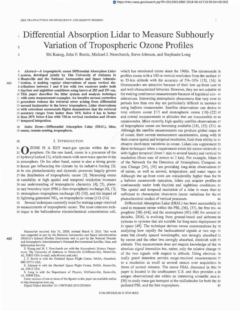
228 constant. Ratios that are not constant ~uggest cltheJ an incorrec.t 229 background subtraction or a wrong dead-time cOrreLtion The 230 merging threshold of the PC signal is tYPically 20 YHz for 231 the Hamamatsu PMT employed in our low-altitude channel 232 and 20-30 MHz for the EM! PMT used on the high-altitude 233 channel. Because DIAL retrie.als depend on the quality of 234 both 285- and 291-nm signals, we combine the PC and analog 235 signals approximately at the same altitude for both lasers to 236 minimize the retrieval error due to the merging. Examples of 237 the ratio of PC to analog signals and their merged region for 238 the 285-nm signal are shown in Fig. 3. The merging threshold 239 is 20 MHz for both altitude channels. The fifth step involves 240 smoothing the signals to reduce random noise. Our configura-241 tion currently employs a five-point (3 x 150 = 750 m) running 242 average appJied to returns from all altitudes; smoothing reduces 243 the effective vertical resolution to 750 m. 244 After initial processing, an exponential-fit correction re-245 moves SIB from the signal returns. This bias. caused by intense 246 light returns from the near range (also called signal-induced 247 noise), appears as a slowly decaying noise source superimposed 248 on the normal returns. The causes of the SIB are related to the

AQ4 249 regenerative effects such as dynode glow, after-pulsing effect. 250 glass-charging effect, shielding effect, and helium penetration 251 [59J. SIB varies widely with different PMTs. For our case, the

SIB of the EMI 9813 is larger than that for the Hamarnatsu 252 7400. sm can persist for several hundreds of mlcro<econds and 253 can exclt a strong influence on data at the lidar'~ upper range 254 whele both signal and noise count!s become (..ompatahle. With 255 unCOIrected SIB, the raw signal falls off more .lowly at higher 256 altitudes. resulting in lower retrie"ed ozone values. SIB usually 257 has more influence on the ~horter wavelength channel, which 258 falls off more rapidly with "ltltude Unle" a mechanical shutter 259 physically blocks the optical path to the PMT to eliminate SIB, 260 a model must charactellze its behd"or. Cairo et al. [6OJ and 261 Zhao [61J have successfully used a dOUble-exponential function 262 for this purpose Howe"er, thic; COllection increases measure- 263 ment un,ertainl1e~. because both the scaling and exponential 264 lifetime. ale difficult lo determine without additional indepen- 265 dent measutements. A more practical technique is to employ 266 " single-exponential fit to the residual background [42J, [43J, 267 [62J. For the high-altitude channel, the function's coefficients 268 rue dutomatically determined using a single-exponential least 269 squdle, fit to data acquired approximately from 100 to 160 !,-S 270 after data acquisition starts where the SIB becomes dominant. 271 The start dOd length of the exponential fit vary with different 272 channels (either wavelength channels or altitude channels),273 atmospheric structures, and !idar configurations because these 274 parameters affect the intensity of the detected signal. For our 275 low-altitude channel, the SIB is weaker than that of the high- 276 dltitude channel because of the different PMT and weaker 277 signal. Howe,'er, it is difficult to automatically determine the 278 fitting function for the low-altitude channel signal using the 279 least squares fitting method, pruticularly for the 285-nm sig- 280 nal, because the far-range signal after background correction 281 is not completely characterized by an exponential function 282 [Fig. 3(b)J. It is useful to optimize the exponential fitting 283

KUANG Itt af.: DIAL TO MEASURE SUBHOURLY VARIATION OF TROPOSPHERIC OZONE PROFILES 5

2.0 I +

:3 I + + ~ L5

11 J

.~ '4. -;; : ..

- r ' E 1 off""'l't-5 . 1+1 +

" .5l +' • ~ 0.5 '­u Q.

+ ; /Merging altitude

: I + + tt I + + ~

0.0 If .. 1 •• , + ++ , .... , .• It ,

o 5 10 15 Alt (km)

(a)

20 25

2.0 1 + I +

0'

e 1.5 ] + ~ ~~ o ~ ++

~ LO . . ' ,-;;4 ~ .. ! ! $ *f .t~ +: _ .. + I ~ 0.5 J ./Mergin

g altitude c +

0.0 1 ~ ~~~~"';';;""'"~:'-"~~L....~ I o 5 10 15

Alt (km)

(e)

20 25

S ~ .'l • " u Q.

N' 0:

Co !i • h

U 0.

10' il

~{<)·.lcl - --\k'Tg<.d ';lIn31 with sm coo, ~lio.-

kl"ed Illnall> n sm tnrTCl:linn .••••••••

SIBfil _._.-

100

f"" -....

10-2

10" 4

0 5 10 15 20 25 Alt (km)

(b)

-~

',{t&l

l·'(crgcd<ijl.ll [\'.ilhSIBcorn::(;1ill'-

If,.r;...1 .;i.1nai" n sr~) tnrll.'ctlon, ••.

~ SIB fil _._.-

--r,\ 100 ....... -" . ........ . , . ,

10- 2 , , , , 10-4

0 5 10 15 20 25 Ail (km)

(d)

Fig. 3. Examples of signal merging and SIB correctJu.l tor tlK. 285-nm signa; JlJe 10-min averaged data occurred .)t i'3 ()() local time on October 18. 2008. (a) Normaliz.ed ratio of PC to analog after bal.¥ground ane; dead-time correcuom, for the low·altitude channel sipwl. (b) Comparison ot the non-Sffi-corrected signal. the SIB-corrected signal. and the model. 0\'" well as the SIB filling tunction, for ll':e low-altitude sign.d The r.J.odc;1 uses the coincident ozonesonde measurement assuming no aerosoL The SIB fitting function (exp( -1.3 - (\~!; . 2 . 10-1)) was empirically deri~·!d using previol1<;ly retrieved data and coincident ozonesonde measurements. (c) Same as (a) but for the hi~h-altitl;de c;hannu. (d) Same as (b) but for the higt,-altlD.lde channel. The coefficients of the SIB fitting function result from an empirical single-exponential kil'it ~uares fit to the signal acquired from 100 to 160.'1.S atteJ. dsta acquisitlOO statts.

284 function for the low-altitude channel using pre\lOllS rell;eval 285 data and compare the data with coincident ozonesonde profiles. 286 The slope of the logarithm of the SIB fitting function remains 287 for a particular configuration (i.e., outgoing power) and could 288 slightly change for different configurations. Those retrievals 289 corrected using the empirically derived exponential function 290 agree with ozonesonde profiles up to 5 km within 5% bias. 291 Fig. 3 shows the typical effect of the SIB correction and the 292 comparison of the fully corrected signal and the model for the 293 285-nm signal. The model simulation employs the coincident 294 ozonesonde measurement assuming no aerosol.

295 B. DIAL Retrieval

296 Excellent discussions concerning the DIAL technique occur 297 in the publications by Measures [63]. Kovalev and Eichinger 298 [64]. and Browell et al. [39]. The average ozone number density 299 n(r+...1" /2) between range.:; rand r + 6.r can be expressed as 300 the summation of the signal term n(r+A'I' /2}' the differential

backscattering tern} ~ntr+6.r/2) ' and the differential extinction 301

tenn ~n(r+.:l' /2) 302

1) lAb + A' 'fl.(r+Ar/2) = n(r+ .:lr/2) -,- .u.n(r+~r/2) .u.n(r_"Dor/2)· (2)

Om;: can wni:e the discrete forms of the three terms at the right 303 side", follows: 304

1 (Pon(")POff(r+/lr)) n(r+A' ,'.;) 26.rD.O'"03 In Poh'(r)Potl(J,+.6r)

(3)

1 (i3on(r)}off(r+/lr») t.·"tr+/lr/2) - - 2t.rt.<7Q:J In3oh( .. )t3on('+/l')

(4)

6.ne J ) = - _1_ (Ct'on(r+ .6r/2) - Ct'oH(r+.6r '2)) (r+.6.r,2 .6.0'"03

(5)

where the subscripts "on" and "off' represent the online 305

(285 nm) and offline (291 nm) wavelengths, respectively. P is 306

tbe detected photon counts. /1 is the total backscatter coefficient, 307

6 IEEE TRANSACTIOKS ON GEOSCIENCE AND REMOTE SENSING

12, 12 f

Sonde Sonde ~.~. i lOf ~ Joined -10 C '" High-dt ...., , ...... Low-alt-

a , ....,

' . a ~

S-S- , '-

6 a ~ 6 6 ~

:L)o~,j " ~

01 4

2c I

2.0 00 0.5 . -3) 1.5

. 0 (1012 molee em

0' 0.5 1.0 -3

3 (b)

0.0

03 (1012 molee em ) (a)

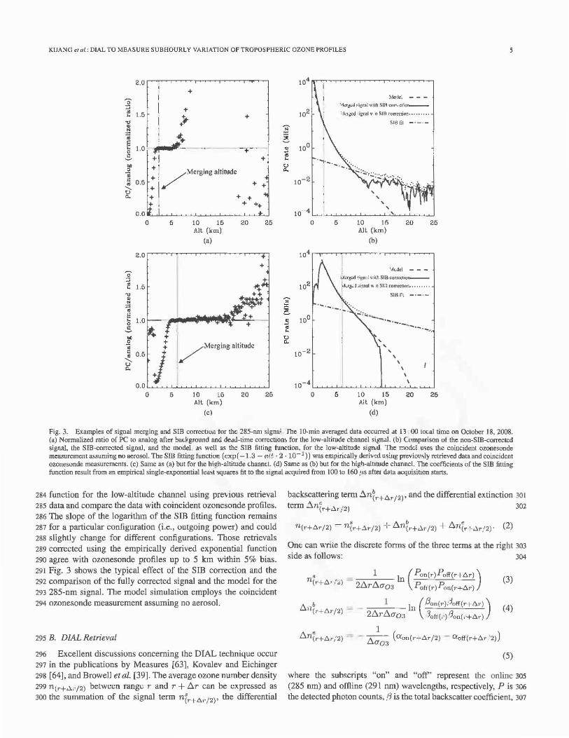
Fig. 4. Example of a joined ozone retrieval for the tidar data in Fig. 3. (a) Separate retrierah. of the two altitude channels. The error bars represent the one-sigma statistical uncertainties. The gray envelope repr.:sents ±lOfk uncertainty of the coinciclent ozonesonde profile. (b) Joined DIAL retrieval from the two altitude channels and its combined one-sigma statistical uncertainty.

308 a is the total extinction coefficient excluding ozone, and 6.0-03

309 is the differential ozone absorption cross section. P, ,3, and 310 a are dependent on r and the wavelength. Strictly speakmg, 311 ~cr03 is T dependent as well because his a function of tempera-312 ture, which varies with r. By ignoring the differential scattering 313 and extinction from non-ozone species, the DIAL equdtlon re-314 duces to only n 8

• ~nb arises from aerosol differential bacl:~cat-315 tering. tine consists of differential Rayleigh extInction, aelO801 316 extinction, and non-ozone gaseous absorption. mcluding O2:

317 S02, and N02. Measurements from a meteOlological sounding 318 can usually correct Rayleigh effects. We correct the aerosol 319 effects when they are significantly enough, jJarticuhlly in PBL. 320 The aerosol correction discussion appears in !:;ectlon ill-D.

321 C. Joining Retrievals From Two Adjacent Altitude ChannEls

322 Final retrievals result from joining the data from two altitude 323 channels with a weighted average. We choose to join the final 324 ozone retrievals instead of the raw signals becau~e the SNRs of 325 the two altitude channels at the joining altitude are significantly 326 different. If the retrievals derived from two different channels 327 are statistically independent, the best estimate of these measure-328 ments is the two-channel weighted average [65]

2 2

nbe<>t -=- L W i ni / L 'U'i (6) i=l i=l

329 where Hi is the ozone retrieval of channel i and the weight 'U'i

330 is the inverse square of the corresponding statistical uncertainty 331 (Oli, which will be discussed in Section V)

Wi = l/cii'

332 The uncertainty of nb(st is

(

2 ) -1/2

Clb(<;t = ~ 'll'i l =l

(7)

(8)

Typically. the low- and high-altitude channels join between 333

3.3 an~ 4 4 km. Fig 4 shows an example of a joined ozone 334

profile, a~ well a~ the combined one-~lgma statistical uncer- 335

tainties. 336

D. Aerosol Correction 337

In a polluted area, aerosols can be a dominant enor source 338

in the lower troposphere. Based on (4) and (5), the vertical 339

gradIent of aerosol backscattering detennine~ Llnb , and the 340

magnitude of the differential-aero~ol extinction coefficient de- 341

tennines Llne. The largest aero.;;ol ('orrection wmally occurs in 342 an inhomogeneous aerosollayel (I.e., the top of the PBL). One 343

can solve for the ozone and aerosol profiles simultaneously with 344 only two wavelengths by assuming dppropriate Angstrom expo- 345

nents and constant Mal latios [66], 167]. If a third wavelength 346

is available and is dose to the DIAL wavelength pair, one can 347 use the dual-DIAL technique [68], [69] to reduce the error due 348

to aelOsol When the third wavelength is far from the DIAL 349

'1yoclvelength pair, one can use the method suggested by Browell 350

et al. [39] to '.:orrect the aerosol interference. Without the third 351

wavelength, we employ an iterative procedure to retrieve ozone 352 md l.onect aerosol effects. To illustrate this method, start with 353

the ~qu'ltlon for ozone number density using only the 291 -nm 354

signal [63] 355

'I1,(r+.6.r/2)

1

20"03 Llr

x {In ( PC") )_In[-,-----''--':((3t:-'--)+p.::..:J,~))!_;_/r-2 _] p(>·+lJ.r) (i);Vf +(3A )/(r+t.T')2

. (r+~r) (r+.6.r·)

-2 (at:+lJ.r/2) + at+lJ.r/2)) t.r} (9)

KUANG ell/f.: Dl:\L TO ME.\SURE SUBHOURLY VARIATION OF TROPOSPHERIC OZONE PROFILES 7

356 where 0"03 is the ozone absorption cross section, !3t:> and 357 t3t) are the molecular and aerosol backscatter coefficients at

358 range r, respectively, and o:t:+ .6.r/ 2) and Cl't+.6.r/2) represent 359 the average molecular and aerosol extinction coefficients, re-360 spectively. between range rand r + /';.r. The subscript 291 361 is omitted for brevity because all backscatter and extinction 362 parameters correspond to 291 nm. Solving for 131;). (9) becomes

.Bt) ~ pxp {In (p p(c) ) - 2n(cHu':2)CTO'/';.'· (,·+..c,.r)

( M + .. 1 ) :,r} 2 fr(r-:-.6.r/2) Ct:(r+.6.1'/2)

r' (.9t:+1> .. ) +q~+1>r)) _ pM. (10) X (r + /';.r)2 (c)

363 Assuming that the lidar ratio (aerosol extinction-to-backscatter 364 ratio). i.e .• S = aA/pA. is known for the 291-nm signal and 365 further assuming that

O(~+1>c:') "" o(:.+1>c) = Sq~+1>c) (II)

366 (10) only contains the following two unknown variables the 367 aerosol backscatter coefficient JC+.6.r) and the ozone number 368 density n(r+.6.ri2) . Molecular backscatter and extinction r:;an be 369 computed from nearby radiosonde data or from climatology. 370 For the first iteration step, n(r+~r/2) can be computed hom 37t (3) and inserted into (10). By assuming a start yalue pecC) at a

372 reference range and a constant S with range~ ill;) can be \olved

373 by (10). Then. the first !3t) profile is subsututed back tnto (10) 374 to compute the second estimate by using a more aCCulate fonn

375 for a:t'+.6.r./2) as

A ( .1 ") / ct(r+ .6.r/ 2) = S _"3(r+~T) + B(71 2 (12)

376 where p(~') represents the value from the fir~t I!~rimate_ With 377 several iterations of (10) and (12) (we name thIS Iteration the 378 "aerosol iteration"), we ca.n get a stable solution for 13(r}' which 379 does not zhange significantly from one iteration step to the next. 380 The aerosol iteration stop criterion is defined as ~a) < ~~in· 381 ~a) is the relative total difference of the backscatter coefficients 382 between two adjacent iteration steps and is defined as

€(1) = 1 rref

C, . , - L I.B·I. - ,I 1 L: q A . ~ , . ( •• 1) P(c.I+l)

r=T, (r ,i) _J

(13)

383 where l represents the iteration step, T ~ is the starting range 384 of the !idar retrieval, and P{: . .l ) are the backscatter coefficients

385 at range r and iteration step l. {;!in is typically 0.0 L for our 386 aerosol retrievals. Aside from {~in' the number of iterations 387 required for a stable solution is also related to the range res-388 olution of the signal. For simplicity. we assume that the power-389 law dependences with wavelength for the aerosol extinction 390 and backscatter coefficients are the same although they can

be different theoretically. L~:;t~r+ .6.r) and D.n{r+.6.r) can be 391 approximated as [39] 392

b _ (4 -1]) /';.>. (B(r) /';.a(,·+"r)- 2/';.r/';. CT03>'off I+B(c)

B(. -+1>,') ) (14) 1 + B(T+".·)

e /';.>. ( A M ) 6.n(r+.6.1·) ~ - D.aOJAoff 7]Q(r+ Ar/ 2) + 4a(r+.6.r/l) (15)

where 1} is the Angstrom exponent, .6.A is the wavelength 393 separation, and B(r) is the aerosol-to-molecular backscatter 394 ratio at the offline wavelength defined as 395

B(,) =.3t/'3t~ (16)

The estimate for the aerosol-corrected ozone number density 396 profile is then substituted into (10) to calculate an updated 397 aerosol baGkscatter profile, which, in tum, is used to compute 398 an updated aerosol-corrected ozone profile. This iteration is 399

name.(1 "ozone iteration" to be distinct with the coupled aerosol 400

iteratIon procesl) A similar iteration stop criterion, ~~: < ~~rn, 401 a~ the aerosol Iteration. can be defined for the ozone iteration 402

by replacing the backscatter coefficient in (13) with the ozone 403 number density. Typic..dlly. only two ozone iterations are re- 404

quired when ~~~n i!) ~et equal to 0.00 J. 405

The lidal rdtio (S) exhibits a wide range of variation with 406

different aero~ol iefractive indexes. size dJ",tnbutions, and hu- 407

IDldity [70] The S measurements have been made most fre- 408 quentIy at 308 [71] and 355 nm [72]. [73] . The S tor our DIAL 409 wavelengths was assumed to be 60 SI-1 [74] constant over the 410 measurement range for typical urban aerosol"> The Angstrom 411 ~:r..ponent (7]) is often seen as an mdicator of aerosol particle 412 SILe o Values greater than two corre!':lpond to small smoke parti- 413 cles, and values smaller than one corre~pond to large particles 414

like sea salt [75]. [76]. Mo.,t of the reported 11\ for tropospheric 4t5 aerosol are measured at \\"avelength~ longer than 300 nm with 416

a variation from zero to two [77]. [78]. Considering that 1] 41 7 could be relatively 'n,all when it is applied in the UV region. 418 we assume that 11 = 0 .5 dt our DIAL wavelengths for urban 419 aerosols [791. 420

SirnulatJoru. were ..:onducted to investigate the aerosol cor- 421 re<.t.J.on in thl! DIAL retneval under an extremely large aerosol 422 gI adient conmnon by a~~uming the aerosol, molecular, and 423 •. ).Lone extinctIon profiles at 291 nm shown in Fig. 5. The 424

h}pott,.etic.ti aerosol profile includes the following three basic 425 regimer.; homogeneous, increasing. and decreasing extinction. 426

The aelO~ol extinction coefficients are set equal to 10- 5 m- 1 427 below 1.2 km and above 3 km to represent a background value. 428 The resulting .teep gradient between the low background and 429 high aerosol value provides an extreme test for the aerosol cor- 430 rection algorithm. The molecular extinction profile is derived 431 from the 1976 U.S. Standard Atmosphere [80]. The assumed 432 ozone extinction profile is constant with altitude and is based on 433 a number density of 1.5 x 1012 molec · cm-3 and an absorption 434 cross section of 1.24 x 10- " cm'· molec- 1 at 291 nm [81]. 435

Fig. 6 shows the comparison of the ozone retrieval both 436 with and without aerosol correction, as well as the calculated 437 aerosol profile, at 291 nm. This example calculation assumes 438 that 1] = 0.5 and S = 60 sr- 1 are known exactly. and there 439

,

8'

4.: .. :. :1 :. :1

38 " ; 1 :1 :1 :1

,.!I: 2r:1 - :1 ..-:;;: :1

:1

o r :" 0.0 0.5

Aerosol --Molecular ..... .

03 - --

1.0 1.5 2.0 Ext. Cae!!. (10-3 m-I)

2.5

j l

j 1

3.0

Fig. 5. Aerosol, molecular, and ozone extinction coefficienl profiles at 291 run for a model calculation of extreme aerosol effects.

8'

o 4

3

,\erosol exL coeff. (lO-3 m - l)

2 3

Aerosol model····· ·· Calculated aerosol 6.

03 model - - -03 w/o aerosol corr. -' _ ..

. _,-,-·-'j03 with aerosol com

··<~··~···~·t··· .... '4 4 .0.

32 ~ 4 4

-, 4

........ -A. ) .'

J ~

••.••••••. •. LJ. •. ••••.•• -~ .-.-.-

O~L~~~~~~~~

o 2 3 03 (1012 molec em - 3)

Fig. 6. Comparison of the simulated ozone retrieval without aerosol correc­tion against that with aerosol correction using the iterative prooedure. The Angslrl:)m exponent ('7) and lidar ratio (8) were assumed to be cxact:y known at 0.5 and 60 5(- 1, respectively, for the aerosol correction. The acrosol correctior. drnmatically improves the ozone reb·ieval.

440 is no signal measurement error. With a range resolution of 441 150 m, two ozone iterations produce the final aerosol-corrected 442 ozone retrieval by setting ~~fn = 0.001. In the process of cal-443 culating the aerosol profile, aerosol iterations produce a stable 444 aerosol solution by setting ~~in = 0.01, which is approximately 445 identical to the model aerosol profile. The aerosol correction 446 procedure reduces the retrieval errors from ±50% to about 447 ±5%. The residual errors are due to the numerical integration 448 and the approximation of (14) and (15). The quality of this 449 iterative procedure depends on the choice of Sand '1. According 450 to (10), (14) and (15), S affects the aerosol profile retrieval, 451 while 1] affects only the final ozone correction. 452 Fig. 7 shows the sensitivity test for Sand 17 in the aerosol 453 correction assuming that S = 60 and ',1 "" 0.5 are the comct

IEEE TRANSACTIONS ON GEOSCIENCE AND REUOTE SENSING

e

4[~~~~~~~~~~-r--~~~~

3 (\

Mockl - - -S '-60. '1~ 0.5 --

S· 60, '1,·· 0· ....... · S·<60. '1=1 _._._.

5'-'40 • .., -0.5 -­S=8O, '1~ 0.5 - -

32 :Oii

.,~, " . ..

o~t~~~~~~~~~~~~~ O~ 0.5 1.0 1.5 3.0 2.0 2.5

03 (1012 molcc em-3)

Fig. 7. Ozone retrieval using differenl Angslrtirn exponents (7/ = 0, 0.3, and 1) and lidar ratios (8 = 4C, 60, and 80) in the aerosol correc.ion.

\-dlues. [naccw ate estimates of S or 1] can yield retrieval errors 454

up to about 20%. Larger 1] will overestimate tl.nc . which 455

produ(.e~ less ozone. and vice versa. r, has a smaller impact 456

on tl.lIb relative to ~ne due to the 4 - 1] factor. The impact 457

of .'3 is latger iTt the inhomogeneous aero$ol layer than in the 458

homogeneou."i l.lyer. The peak error is large! for underestimated 459

f; relative to o,erestimated S [82]. 460

We summarize the iterative procedure as follows. 461

I) Calt.ulate the first estimate of the Olone c.oncentration 462

from (3). 463

2) Substitute the first estimated ozone into (10) to derive the 464

aerosol backscatter profile fOI the offline wavelength, and 465

iterate to obtain a stable solul100 with (12). 466

3) Calculate the differenllal aerosol baLk ,catter and extinc- 467

tion corrections to obtain d c;econd estimate of ozone 468

using (14) and (15). 469

4) With the se<-ond Olune estimate, go back to step 2. 470

IV. MEASUREMENTS 471

Fig. 8 shows an ozone DIAL retrieval for 15 consecutive 472

hours from 12: 56 local tune, August 9, to 03: 56, August 10, 473

2008, with lO-min temporal integration (12 ()()() shots) and 474

750-m vel tical range resolution using the data processing de- 475

scnbea In the previous section. The aerosol correction was 476

made only at altitudes between I and 4 !un using the data 477

from the low-altitude channel because of the negligible aerosol 478

effects abO\e 4 km. The aerosol time-height curtain [Fig. 8(a)] 479

exhibits moderate aerosol activity below 2 km with expected 480

diurnal PBL variation and shorter timescale fluctuations due to 481

PBL processes. The maximum aerosol correction in Fig. 8(b) 482

corresponds to an ozone adjustment of 3-4 ppbv and occurs 483

between 1.5 and 2.5 km for the largest vertical backscatter 484

gradient. The retrievals for the two altitude channels overlap 485

between 3.3 and 4.4 km to produce the final ozone profiles 486

[Fig. 8(c)] that agree well with the colocated ozonesonde (EN- 487

SCI model 2Z with unbuffered 2% cathode solution) launched 488

at 13: 49 local time. The time-height curtain of ozone's 489

KUANG tt :11.: DIAL TO MEASURE SUB HOURLY VARIATION OF TROPOSPHERIC OZONE PROFILES 9

10"' m" "'Q 2.26

.- 2.00

- 1 .~

! ., ~ 1 • 'M · , ... • '.(10

f .71'-

' ... 0.£3

r.oo

" I ~, " " " " ., " ..2 ., 00 " " " 1.m~ (c "n 10 ' u.-.2008

(a)

sF' '1 _ 10

•

!l J

r • · , · , · 0

· ., . t- U · . ,

. .,; . ,

o{;. , ~ 11.." " .. " " !. Ie "

2Q " .,. '" 00 01 oz 03

TJmt (r ~J) :0 ... ".-. ;>()()(;

(b)

., .. :f7~;

. '...;: i f'-' ......!.r ,_ , "1"" ' .... :-.::Jo' 1] . • - 120

" _110

~-"o ."

~ :-:-.

~ ~ ." " " ..

o b::J • ' 3 14 ,. ,. ,7 '8 ,. ' 0 " 22 '"" 00 ., ., 03

T:r.'~ .CDT; 10 "'''1. :-00:'

(e)

Fig. 8. Ozone DIAL retrievals made on AuguSl9-lO, 2008. (a) Calculated aeLO.,ol extinction r...(I(;fficient at :l91 run. The feature tit 2 km, 14 : 00 is a cloud. (b) Aerosol correction for ozone DIAL retrieval. (c) Ozone DL\L retrieval tlfter a~lOl,Ol con-ection The retrieval was made with a 75D-m vertical range resolution and a IO·min temporal resolution. The colocated ozonesonde lJUlrl<ed by a triangle \ltd'. launched d( 13: 49 local time.

490 evolution shows a very interesting structure of multiple ozone 491 layers in the lower atmosphere that varies with time. One can 492 see the buildup and decay of various layers throughout this 493 12-h penD<!. The high-frequency mriation in the high-altitude 494 channel ( ~ 6 km) results partly from lower SNR and higher 495 uncertair:ty of the SID correction, both of which increase with 496 altitude. Fig. 9 shows the mean ozone profile and one-sigma 497 standard deviation for the I Q-min vertical profiles between 498 12: 56 and 15 : 06 local time in Fig. 8, as well as the coinci-499 dent ozonesonde measurement. The high-altitude channel has a 500 standard de.viation increasing with altitude due to the statistical 501 error distribution. Its standard deviation is less than 13 ppbv

below 8 km and increases to about 45 ppbv at 8.5 km where the 502

285-nm lasel does not have sufficient SNR for ozone retrieval; 503 AQS

therefore, we terminate the retrie\als at 8 km in Fig. 8. The stan- 504

dard deviation of the low-altitude channel retrievals is less than 505 5 ppb\ below 4 Jan and reaches 8 ppbv at 5 km due to lower 506 SNR. The standard deviation at 2 km is a little larger than the 507 surrounding altitudes possibly because of larger ozone fluctu- 508 ations or larger uncertainties of the aerosol correction in the 509

ozone retrieval at the PBL top. The two altitude channels have 510

consistent mean retrievals in the overlap region with discrepan- 511

cies less than 5 ppbv and similar standard deviations at 3.3 km 512

which most likely reflect the true ozone short-term variations 513

10

II)

B

- S S =-~ :;;: •

2

°0

r"''.' .. .' "

.'

Sonde ... High-a.ll Low- alt --

00 100 150 03 (ppbv)

Fig. 9. Mean ozone mixing rutio and one-sigma standard d .... vialion for the IO-min venical profiles between 12:56 and 15 :06 local time in Fig, 8. The colocated ozonesonde was launched at 13: 49 local time. The large en'Or bar ("-'45%) tll 8.5 krn identifies the high-altitude limit of the retrievals (8 xm),

514 above the PBL as shown in Fig. 8. The mean retrievals agree 515 with the ozonesonde measurement within about 10 ppbv and 516 have higher biases at the upper altitudes,

517 V. ERROR ANALYSIS

518 We divide the error budget of the DIAL retrieval mto the 519 following four categories: 1) statistical uncertainties £1 art"ing 520 from signal and background noise fluctuation" l) errOIS £;.

521 associated with differential backscatter and extmction of 000-522 ozone gases (0,. SO" NO" etc.) and ae1O,ols; 3) errors "3

523 due to uncertainties in the ozone absorption cross sec.tIOn; and 5244) errors £4 related to instrumentation and electroruc~. £ 1 is a 525 random error; c2, C3, and c4 are sy.stemau(, errors. cl can be 526 written as [41]

<1 = 2nLl.r Ll.u o 3 1

L (SNR'A'~ ' i,>'

(17)

527 With the assumption of a Poisson distribution gm·erning PC, 528 the SNR at wavelength A and range registration j becomes

P A SNRn = J, , (Pj,A + p. + PdP /2

(18)

529 where Pb is the solar background counts and Pd is the dark 530 counts. It is straightforward to show that cl is proportional 53 1 to (Ll.r'NApL)-1/', where N represents the total number of 532 shots, A is the unobscured area of the telescope's primary 533 mirror, and PI .. is the number of emitted laser photons. !:l.r 534 must be chosen large enough to produce an acceptably small 535 error. Fig. 10 shows the estimated statistical errors for the 536 high- ar.d low-altitude channels for a IO-min integration and a 537 750-m range resolution. t'l is typically less than 1O<7c below 538 4 km for our low-altitude channel and could be 20'k at 5 km. 539 This altItude performance gives us sufficient overlap for the 540 two altitude channels under most atmospheric conditions. In 541 the high-altitude channel, £1 exceeds 25% of the retrieval ozone 542 near 8 ± I km, where we terminate the retrievaL

IEEE TRANSACTIONS ON GEOSCIENCE AND REMOTE SENSING

10 [ , . (.' '::::::::::=l

B

_ 6

5 C ;1

Nighttime Daytime

Summer daytime

OL'~~~~~~~~~~~~~~~

o 10 20 30 40 50 Percentage error (%)

Fig. to. p. .. umated statistical errors for the high- :md low-:JltilUde channels using IO-min integration and 750-m range resolution. The nighttime and daytime statistical errors are modeled by using the annually av.::raged local o7.on~,~onde profile the 1976 U.S. Standard Atmosphere, an urban aerosol model [83], and the !idar panmeters in Table J. The ozone profile used for summer daytime errors is assumed 20% higher than the annual average.

E2 lOcJudes the interference from O2, S02, NO:.l1 air mole- 5.+3 cules, and aeroso}!.; Table II summarhes the potential errors 544 in the DIAL rctneval for 285- and 291-nrn wavelengths due 545 \(, non-ozone absorption gases [84]-[88] The calculation of 546 the oxygen dimer (02- 02) interference mdudes some un- 547 certaintif,!) due to the absorption cross-~tionaJ me-3surement. 548

The 02 - 0, absorption theory has not been entirely e'tablished 549 [89], Local SO, and NO, profiling data are not availahle. How- 550 ever, the estimated error due to eIther 502 or N02 using the 551 latest ground observation is less than I %. The impact caused by 552

differential Rayleigh extinction resl1lts in an in;,.ccuracy of less 553 than 1 % using balloon ozone~onde letnevals of atmospheric 554

density or by employing climatologIcal models, 555

The main concern ('omes from the aerosol interference, 556

which depends on both the wavelengths and wavelength sep- 557 aration. Altnougn the aelOwl opllcal properties could be re- 558 trieved from a thud wavelength, the differential effect for a 559

DV\L wa,e\ength pair stil1 has some uncertainty due to the 560 al)sumption for lidal tdtio and Angstrtlm exponent. Within the 561

PBL, where the statistJc.dl errors are sman, differential aerosol 562

backscattt''llllg and extinction dominate the error sources [39], 563

[41]. [431 However, it is reasonable to believe that the error 564 due:. to aerosol interference is smaller than 20% a.~er the aerosol 565

correctIon, as shown in Section III-D. 566

The ullcertainty in the Bass-Paur ozone cross sections is 567

believed to be less than 2<Jt [81], [84], [89]. <, will be less than 568

3% after considering the temperature dependence. 569 C,J could be caused by a misalignment of the lasers with 570

the telescope FOV, imperfect dead time, or SIB correction, 571 Dead time distorts the near-range signal, and SIB distorts the 572 far-range signal. Because the dead-time benavior is reliably 573 characlerized, the error caused by SIB usual1y is larger than 574 the dead-time error. These errors related to the signal non- 575 linearity can be experimentally diagnosed by a fllnction- 576

generator-driven LED laser simulator [90], [91J, For the lO-min 577 integration data, C4 is estimated to be < 5% at 1-4 km for our 578

KUANG nal.: DIAL TO MEASURE SUBHOURLY VARIATION OF TROPOSPHERIC OZONE PROFILES 11

TABLE 11 DIAL RETRIE':.\ L ERRORS DLE TO NON·OZONE AaSORPTION GA SES

Gases 1'1 a , differential

absorption cross-section (cm2 molec· 1) for 285 and

291 nm

03 1.15x lO- 18

O{I 4.5xIO-21

S02 _4.8xI0-20

N02 _2.25xlO-2o

References

for 1'1<7

Bass and Pallr 198 1

[84]

Fally et al. 2000 [85]

Rufus et al.

2003 [86]

Bogumil et .1. 2003 [87]

Mixing ratio Reft:rences for D3 retrieval

(ppbv) mixing ratio error (%)

60

2. lxIO· 1.5%

13b NREM2oo6 -0.9%

[88]

18' NREM2006 -0.6% [88]

Total ±1.5%

I due to <r.!.<r.! b maximum 24-hr awrage in 1994. Latest local monitollDg data available. C Annual arithmetic average in 1993. Latest local momtoring data a"·81lable.

TABLE III SUMMARY OF THE ERRORS IN RJ\PCD OZONE DL\L MEASURh:..tE:-.lTS

Errors Low-altitude channel

( l-4 lunl

High-altitude channel (3-8km)

I. E,_ statistical error

2. E2• interference by non-ozont! ~pecies Aerosol Non-ozone absorption ga~es Rayleigh

3. £3 , due to uncertaint) In 6.aOJ

4. £4 ' due to SIB and dEad-time

Total RMS error

-:: 10% -::25%

-::20°10 .-:5% <1.5°0

.:.: 1 ~·o using local radiosonde profile ~3~o

<5%

<23%

< 10%

·'28%

• The errors are estllnJted by a~uming a 60 ppbv constant ozone mixing ratio 111 the troposphe1e for data wid} a 750-m · .. el tical resolutIOn dlld lO-min integration.

579 low-altitude channel and ~ 1090 for our high-altltude channel 580 below 8 kIn based on our LED test results and the analysis of 581 our previous data such as Figs. 8 and 9. A summary of the errors 582 in the DIAL measurements is shown in Table [IT for a constant 583 troposphoric ozone of 60 ppbv. 750-m vertical resolution, and 584 lO-min iiltegration. 585 Fig. 11 shows a comparison of 12 lidar retrievals and their 586 single coincident ozonesonde measurement between 13 : 00 and 587 14: 00 local time except for the first profile on August 17.2008 588 (upper right panel). which was taken at 08: 00. The aerosol 589 correction was made at altitudes between I and 4 km by setting 590 the reference altitude at ~6 kIn and Pi~d) = 1.67 X 10 7 m~l .

591 SC' [83J. Fig. 12 shows the mean percentage differences and 592 their star~dard errors of the mean for all those retrievals. The li-593 dar retrievals of the low-altitude channel agree with ozonesonde 594 measurements within 10% from 1 to 4 km. The relatively 595 high errors at about 2 kIn possibly relate to residual aerosol 596 correetio!) errors around PBL height. The lidar retrievals from 597 the high-altitude channel agree with ozonesonde to within 20'10 598 below 8 km. The statistical error and the uncertainty associated

with the SIB cOllection result m larger eITors for the high- 599 altitu,l.e channel abo.e 6 kIn. 600

VI CONCLU~JON ~\ND FUTURE PLANS 601

The R>\PCD ozone DIAL system measures tropospheric 602 ozone plofiles during bolh daytime and nighttime using the 603

285-/291-nm wavelength pair. The low-altitude receiving chan- 604

nel make~ Olone measurements at altitudes between 1 and 5 kIn 605 using a IO-cm (elescope and Hamamatsu R7400U PMTs. The 606 high-altitude channel measures ozone between 3 and about fIJ7

8 kIn using a 40-cm telescope and EM! 9813 PMTs. Model 608

calculations demonstrnte that the iterative aerosol correction 609 procedure significantly reduces the retrieval error arising from 610 differential aerosol backscatter in the lower troposphere where 611 the quality of the aerosol correction depends on the accuracy of 612 the (I. priori lidar ratio and Angstrom exponent. A comparison 613 of the lidar retrievals and coincident ozonesonde measurements 614 suggests that retrieval accuracy ranges from better than 10% 615

after the application of an aerosol correction below 4 km to 616

12 IEEE TRANSACTIONS ON GEOSCIENCE AND REMOTE SENSI:"l"G

101000

•

8/11/2008 8/14/2008 8/15/2008 8/16/2008 8/17/2008

... - ,: / ::. \/ 8 'J , ....

' ...

, :1 I.'

.' ! .• '

i ,.! ,

~ e {" ~ :\;

'\ \ \ \ t, ,

21 \ 0 1 , .' 1

0 1010001012

8/17/2008 10/4/2008 iO/18/200B 10/25/2008 11/1/2008 11/8/2008

10 ..... ~ f' '~ ), t··~··· /( I

8 .. , : ) t. \ /'

.~ \ \\ \ ( \ E 6 6 :;;: .

2 \ '\ ~ ) \ } 0 1 ' , o o o 1 0 1 0 o 2

0-: (1 012 moJec cm-1)

Fig. I J. Comparison of the (solid) low- and (dashed) high-altitudr.-(,ha.'1nel aerosol-(,orrected reOlehllr. with the (dotted) coincident OLOnt;~onde measurements.

10r~~~"""""~'-"-'-'-~~

e

E 6 ~ ~

:;; 4

2

f··· :. - - - .-- - . , ' , _ ~ ~.-:~:;"':;'" _ J. _

. i ~ Low-alt --

- -"'--.::.;-- I High-alt- _. , , , .

~

)

o[~~~~~~~~~~--~ -20 -10 o 10 20

Mean percentage difference (%)

Fig. 12. (Dark) Mean percentage differer.ces, lidar sonde/sonde. and (gray) their eslinated one-sigma standard error of the mean for the data in Fig, II.

617 better than 20% for altitudes below 8 km with 750-m vertical 618 resoiuti.1n and lO-min integration. Error sources include 5ta-619 tistical uncertainty, differential scattering and absorption from 620 non-Olone species, uncertainty in ozone absorption cro~s sec· 621 tion, and imperfection of the dead-time and SIB corrections. 622 The uncertainty in the SIB correction and the statistical errors 623 dominate the error sources in the free troposphere and could be 624 reduced by increasing the integration time or reducing the range 625 resolution. 626 Future improvements will overcome two major limitations 627 of the current system by doing the following: I) cxtending 628 observations into the upper troposphere by replacing the current 629 transmitters with more powerful ones and shifting the current

wavelength, to longer ones to make higher-allttude nighttime 630

measurements and 2) minimizing aero"<ol interference in the 631

lowe! troposphere by adding a thIrd w",elength (dual-DIAL 632

techmque). This lidar with expected improvem~nts will provide 633

• unique data set to investigate the chemical and dynantical 634

processes in the PBL and free tropo'phere. The spatiotemporal 635

variance estimates derived nom the Olone hdar observations 636

will also be useful fm d~sessing the variance of tropospheric 637

ozone captured by sateliIte retrieval; 638

ACKNOWLEDGMENT 639

The auth(",; would like to thank T. McGee, S. McDerntid, 640

and T. Leblanc fOl the extensive discussions, 1. Kaye, 641 P. K. Bharlta and R. McPeters for the continuing support, 642

dIld the UAHuntsviHe ozonesonde team, namely, R. Williams, 643

P. Buckley, and D. Nuding, for providing the ozonesonde data. 644 The authors would also like to thank W. Guerin for editing the 645

manusCllpt. 646

REFERENCES 647

(II D. Jacob. Introduction foAtmosph,~ric Chemistry. Princeton. NJ: Prince- 648 ton Univ. Press. 1999, pp. 199-200. 649

[21 D. Shindell. G . Faluvegi, A. Lads, J. Hansen. R. Ruedy. and E. Aguilar, 650 "Role of tropospheric ozone increases in 2Orh-century climate change," 651 J . GeophJs. Res., vol. III. no. D8, p. 008302. Apr. 2006. 652

(3) J . Lelieveld and F. J. Denlener. "V: hat controls tropo.'ipheric ozone?," 653 J. Geol,hys. Res. , vol. 105, no. D3, pp. 3531- 3551, Feb. 2000. 654

[4] J. Stutz. B. Alicke. R. Ackellrn1lln. A. Geyee, A. White, and E. Williams, 655 "Vertical profiles ofN03. N20fj , 0 3. nnd NO;, in the nocturnal bound- 656 ary layer: 1. Observations during the Texas Air Quality Study 2000," 657 J. Geophys. Res .• vol. 109. no. 012, p. D12 306, Jun . 2004. 658

KUANG etat.: DIAL TO MEASL' RE SUBHOURLY VARIATION OF TROPOSPHERIC OZONE PROFILES 13

659 [5J A. Geyer and J. Stutz., "Venical profiles of N03. N2:0s. 03, and NOx in 660 the nocturnal boundary layer: 2. Model slUdies on the altitude dependence 661 of composition and chemistry," 1. Geophy.f. Res., vol. 109. nco 012, 662 p. DI2 307. Jun. 2004. 663 [61 J. Liang, L. W. Horowitz, O. J. Jacob, Y. Wang, A. M. Fiore, J. A. Logan. 664 G. M. Gardner, and J. W. Munger, "Seasonal budgets of reactive nltrogen 665 species and ozone over the United States, and export fluxes to the global 666 atmosphere." 1. GeopllYs. Rt'S.. ':01. 103, no. OIl. pp. 13435-i3450. 667 Jun. 1998. 668 [7] W. B. Grant, E. V. Bmwell, C. F. Butler, M. A. Fenn. M. B. Clyton, 669 J. R. Hannan, H. E. Fuelberg. O. R. Blake, N. J. Blake, G. L. Gregory, 670 B. G. Heik('~, G. W. Sachse, H. B. Singh, J. Snow, and R. W. Talbot, 671 "A case study of transport of tropical marine boundary layer and (O\',er 672 tropospheric air masses to the northern midlatitude upper tropos;mere," 673 J. Geopllys. Res .• voL 105. no. D3. pp. 3757-3769. Feb. 2000. 674 [8] H. Eisele, H. E. Scheel, R. Sladkovic, and T. Trickl, "High-resolu:ion Ii-675 dar measurements of stratosphere-troposphere exchange." 1. Atmc.s. Sci., 676 vol. .56. no. 2, pp. 319- 330, Jan. 1999. 677 [9] A. Stohl, P. Bonasoni, P. Cristofanelli, W. Collins, J. Feichter, A. Frank, 678 C. Forster. E. Gerasopoulos, H. Gaggcler, P. James. T. Kentarchos, 679 H. Kromp-Kolb, B. Krtlger. C. Land, J. Meloen, A. Papayannis, 680 A. Prilter, P. Seibert, M. Sprenger, G. J. Roelofs, H. E. Schtt:I, 681 C. Schnabel, P. Siegmund, L. Tobler, T. Trick], H. Wernli, V. Wirth, 682 P. Zanis, and C. Zerefos. "Stra:osphere-tro;>osphere exchange: ,\ review 683 and what we learned from STACCATO," 1. Geophys. Res., vo:. 108, 684 no. 012, p. 8516, 2003. 685 [101 A. O. Langford, C. D. Masters, M. H. Proffitt, E.-Y. Hsie. and A. F. Tuck, 686 "Ozone measurements in a tropopause fold associated with a cut-off low 687 system," GII!'0P;'YS. Res. Letl., vol. 23, 00. 18, pp. 250:-2504,1996. 688 {II] A. J. DeCana, K. E. Pickering, G. L. Stenchikov, and L. E. Ott. 689 "Lightning-generated NOx and its impact on tropospheric ozone produ(.-690 tion: A three-dimensional modeling study of a stratosphere-troposphere 691 experiment: Radiation. aerosols and ozone (STERAO-.\) thunderstl.um," 692 1. Geophys. Re.~ .. vol. 110, no. 014, p. D14303. luI. 2005. 693 (12] O. R. Cooper, A. Stohl. M. Trainer, A. M. Thompson, 1. \.. Witte. 694 S. J. Oltmans. G. Morris, K. E. Pickering, J. H. Crawford. G (hen, 695 R. C. Cohen, T. lL Bertram, P. Wooldridge, A. Perrir.g, W. H. Smne. 696 J. Merrill, I. L. Moody, D. Tarosick, P. Ned61eL. G. FOf'i-'oe!o 697 M. 1. Newchurch, F. 1. Schmidlin, B. J. John!;;on, S. TU!'Quet). 698 S. L. Baughcum, X. Ren, F. C. Fehsenfeld, J. F. Meagher, N. Spichtinger. 699 C. C. Brown, S. A. McKeen, I. S. McDermid, md r. Leblam .. . 'Large 700 upper tropospheric ozone enhancements above nudlatirude NOIth Amer-701 ica during summer. In silll evidence from the 10",S and MOZ '\IC ozone 702 meascrementnetwork," J. Gcophys. Res., vol. 111 . no 024, p. D24S05, 703 Dec. 2006. 704 [13] O. R. Cooper,M. Trainer, A. M. Thompson, I) T.Oltmau" D W. TaraskJ, 705 J. C. Witte, A. Stohl, S. Eckhardt, 1. lellcveld, M. J NewchuJ(.h, 706 B. J. Johnson, R. W. Portman.'l, L. Kalnajs. M K. Dubey, 1 Lehlanc, 707 1. S. McOemlid. G. Forbes, O. Wolfe, T. Cal(.)···<.imith, G. <\ MOlTis. 708 B. Lefer, B. RappenglOck. E. Joseph, F. Sc.hrm.j1in, J. Meagher. 709 F. C. Fehsenfeld, T. J. Keating, R. A. V. Curen. and K Minschwaner. 710 "EvidL.nce for a recurring eastern North America ilppL~ tropospheric 711 ozone maximnm during summer," J. Geophys, Res., vol. 112. no. 023, 712 p. 023 304, Dec. 2007. 713 [14] U. Schumann and H. Huntrieser, 'The globalligoming-induced nitrogen 714 oxides source," Atmos. Chem. Pliys., vol. 7, no. 14, pp. 3823-3907, 715 2007. 716 [15] S. J. Ol!lnans, H. Levy. ll, J. M. Harris, J. T. Merril!, J. L. Moody. 717 J. A. Lathrop, E. Cue\.ds, M. Trainer, M. S. O'Neill, J. M. Pro.~pero, 718 H. Vt)mei, and B. 1. Johnson. "Summer and spring ozone profiles over 719 the Nonh Atlantic from ozonesonde measurements," J. Geophys. Res., 720 vol. 101. no. 022, pp. 29 179-29200, Dec. 1996. 721 [16] M. J. Nev.'church, M. A. Ayoub, S. Oltmans, B. Johnsor., and 722 F. J. Schmidlin, "Vertical distribution of ozone at four sites in (he United 723 States," 1. Geophys. Re.f., vol. 108, no. DI , p. 4031. Jao. 15,2003. 724 [17] R. O. McPeters, G. J. Lubow, and B. J. Johnson, "A satellite-derived 725 ozone climatology for balloonsonde estimatior. of total column ozone," 726 1. Geophys. Res., vol. 102, no. 07. pp. 8875-8885, Apr. 1997. 727 [18] J. P. Bun'ows, M. Weber, M. Buchwitz, V. Rozanov, 728 A. Ladstatter-Weienmayer, A. Richter, R. DeBeek, R. Hoogen, 729 K. Bnunstedt, K.-U. Eichmann, and M. Eisinger, 'The Global Ozone 730 Monitoring Experiment (GOME): Mission conc.::pt and first scienlific 731 results," J. Atmos. Sci., vol. 56, no. 2, pp. 151 - 175, Jan. 1999. 732 [191 M. J. Newchurch, D. M. Cunnold, and J. Coo, "Intercomparison of 733 Stratospheric A.:.msol and Gas Experiment (SAGE) with Umkt-hr[641 and 734 Umkehr[921 ozone profiles and time series: 1979- 1991." 1. Genphys. 735 Rc.f" vol. \03, no. 023, pp. 31277-31292, Dec. 1998.

[201 M. J. Newchurch. E. S. Yang, O. M. Cunnold, G. C. Reinsel, 736 J. M. Znwodny. and J. M. Russell. lJI . "Evidence for slowdown in 737 strotospheric ozone loss: First stage of ozone recovery," J. Geophys. Res., 738 vol. 108, no. 016, p. 4507, :\ug. 23, 2003. 739

[211 l. M. Russell, III, L. L. Gordley, J. H. Park, S. R. Drayson. W. D. He::;keth, 740 R. J. Cicerone, A. F. Tuck, J. E. Frederick. J. E. Harries, and P. J. Crutzen, 7,11 "The halogen occultation experi ment." J. Geophp. Re.f., vol. 98, no. 06, 742 pp. 10777-10797. Jun. 1993. 743

[22] J. W. Waters, L. Froidevaux, G. L. Manney, W. G. Read , and L. S. Elson, 744 "MLS observations of lower stratospheric cia and 03 in the 1992 south- 745 ern hemisphere \',inter," Geophy.t. Re.t. Lett., vol. 20, no. 12, pp. 1219- 746 1222, Jun. 1993. 747

[23] x. Liu, K. Chance, C. E. Sioris, R. J. O. SPUrT, T. P. Kurosu, R. V. Martin, 748 and M. J. Newchurch. "Ozone profile and tropospheric ozone retrievals 749 from global ozone monitoring experiment: Algorithm description and 750 ':olidntion." J. Geophys. R,.f .. vol. 110, no. 020. p. D20307, Oct. 2005. 751

[24] J. R. Ziemke, S. Chandra, B. N. DunClln. L. Froidevaux, P. K, Bhania, 752 P. F. Levelt, and J. W. Waters, "Tropospheric ozone determined from Aura 753 OMI and MLS: Evaluation of measurements and comparison with the 754 global modeling initiative's chemical transport model." J. Geol)hys. Res., 755 vol.l ll,no.019,p.DI9303,0ct,2006. 756

[25] Y. Choi Y Wang, T. leng. O. Cunnold, E.·S. Yang. R. Martin, K. Chance. 757 V. Thnulet, and E. Edgerton, "Springtime transitions ofN02, CO, and 03 758 oVeJ North America: Model evaluation and analysis," J. Geophys. Res., 759 vol. 113, no. 020. p. 020311, Oct. 2008. 760

[26] Q Yang, D M. Cunnold, H.-J. Wang, L. Froide\aux, H. Claude, 761 T. Merrill, M l'Iewchurch, and S. l. Oltmans. "Midlatitude tropospheric 762 07.o:lC columns derived from the Aura Ozone monitoring instrument and 763 ffil(.roW,a\'t! limb sounde. me.asuremen~," J. Gl'ophys. Res., vol. 112. 764 no OW. p. 020305.0« 2007. DOl: 10. 1 02912007JDOO8528. 765

[27] J. H. KIm. M. J. Ne'hl".hurch. and K. Han, "OlStllbution of tropical tro- 766 posphem. ozone detelmined by the scan-lIngl(. method applied to TOMS 767 measurer.lenh' I \tTr.os. Sci., vol. 58, no. 18, pp 2699-2708, Sep. 2001. 768

[281 1. H. Kim and M. I. Newchurch. "Biomass-but PIng influence on tro- 769 pospheric OZOnt; over New Guinea and Soulh Amt:Il('cl ., J. Geophys. ReJ·., 770 vol. 103 no. 01. pp. 1455-146I,Jao. 1998. 77 1

[29] J. H. KIm S. Na, M . J. Newchurch, and R. V, Maran Tropical tm- 772 posphelK ozone morphology and seasonabt) ~C'n in .l.dtt.llite and in 773 situ m~asurements and model calculations," J. Gwphvs. Re.s . vol. 110, 774 DC, D2, p. D02303, Jan. 2005. 775

[101 '\. Liu. K. Chance, C. E. Sioris, T. P. K.wosu, R. Spurr, R V. Martin, T. Fu, 776 r. Logan, D. Jacob, P. Palmer, M. J. l'Ie\"church, I. A MegrelSkaia, and 777 R. B. Chatfield, "First directly retrieved gloMI distributIOn of tropOSpheric 778 column ozoce from GOME: C.omparison "'·Ilh Ihe GLO~-CHEM model," 779 J. Geophys. Res., vol. III no 02, p D02 ~()f, Tan 2006. 780

[311 X. Liu, K. Chance, C. E Sioris. T. P Kurosu, and M. J. Newchurch, 781 "lntcrcomparison of GOI\1E, ozonesondt . clnd SAGE II measl.:rements of 782 ozone: Demonstration of the need to homogenize a\.ailable ozonesonde 783 data sets," J. GeophrJ R('\. ':01. Ill , no 014. p. 014305, Jul. 2006. 784

[32) R. Beer, "TES on tht:. Aura ml-.sion: Scientlfic objectives, measurements. 785 and ana1ysisovt=l",'lew," IEEE hum (jrasci. RetnnfeSens. , vol. 44, no. 5,786 pp 1102- 1105, Md)- 2006. 787

[33] P r L~elt. E. Hli!)enrath, G. W. Leppelmcier, G. H. 1. van den Oord, 788 ? K. Bhartta. J. Tamounen, J. F. de Haan, Bnd J. P. Veefkind, "Science 789 Objectives of the ozone monitoring instrument," IEEE Traru. Geosci. 790 Remote S,.", vol. 44, no. "i pp. 1199-1208, May 2006. 791

[14J W. Sleinhlu..ht, T. J. McGee. L. W. Twigg, H. Claude, F. SctWnenborn, 792 (j K. ')umnicht, and D. Silbert. " lntercomparison of stl1ltospheric ozone 793 .md tl-mperalure profiles during the October 2005 HohenpeiBenberg 794 Ol.One Profiling Experiment (HOPE)," Armos. Meas. Tech., vol. 2, no. I, 795 pp. 12~-·145. 2009. 796

[35] T. Tridd N B1irtsch-Ritter, H. Eisele, M. Furger, R. Miicke, and A. Stohl, 797 "High-ozone layen; in the middle al1d upper Lroposphere above Central 798 Europe: Shong import from the strato.~phere over the Pacific Ocean." 799 Atmo.f. Chem. Phys. DiscuS.f. , vol. 9, no. I . pp. 3113-3166, Jan. 2009. 800

[36] Y. Zhao, R. D. Marchbanks, and R. M . Hardesty, "ETL's transportable 801 lower troposphere ozone lidar and its applications in air quality studies," 802 Proc:. SPIE, vol. 3127. pp. 53-62. 1997. 803

[371 R. J. Alvarez, II, W. A. Brewer. D. C. Law, J. L. Machol, 804 R. D. Marchbanks, S. P. Sandberg. C. J. Senff, and A. M. Weickmann, 805 "Development and application of the TOPAZ airOOITh: lidar system by 806 the NOAA Earth System Resean:h Laboratory," in Pmc. 24th 1m. Laser 807 Radar e(m/, 2008, pp. 68-71. 808

[38] G. Ancellet. A. Papayannis, J. Pelon, and G. Megie. "DIAL tropospheric 809 ozone meaSlirement using a Nd:Y.\G laser and the Raman shifting 810 technique," J . . HmO.f. Ocetln. Techno/ .. vol. 6. no. 5, pp. 832-839, 811 Oct. 1~89. 812

14

813 [39J E. V. Bmy,ell. S. Ismail. and S. T. Shipley. "Ullraviolel DIAL measure-814 rr:en's of 03 profiles in regions of spatially inhomogeneous nerosols," 815 Appl. Opr., vol. 24. p.o. 17. pp. 2827-2836. Sep. 1985. 816 [40] T. Fukuchi. T. Fujii, N. Cao. and K. Nemoto, ''Tropospheric 0:3 measure-817 me::ts by simuitaneOllS differential absorption !idal" and null profiling," 818 Opt. Eng., vol. 40, no. 9. pp. 1944---1949. Sep. 2001. 819 [411 A Papayannis, G. Aocellet. 1. Pelon, and G. Megie. "Multh.;rave-820 length lidar for ozone measurements in The troposphere and lIle JO\·.~r

821 slnI:osphere," .1pp'. Opt .• \'01. 29. no. 4, pp. 467-476, Feb. 1990. 822 [42J M. H. Proffitt and A. O. Langford, "Ground-based differential absorp-823 tiar. Iidar system for day or night measurements of ozone through-824 oul the free troposphere," Appl. Opt., vol. 36, 110. 12, pp. 2568-2585, 825 Apr. 1997. 826 [43] J. A. Sunesson. A. ApilUiey, and D. P. J. Swart. "Differential absorption 827 lid<:! system for routine monitoring of tropospheric ozone," Apl)l. 01)1 .• 828 vol. 33. no. 30, pp. 7045-7058, Oct 1994. 829 [441 J. L. Machol, R. D. Mnrchbanks, C. J. Senff, B. J. McCarty, 830 W. L. Eberhard, W. A. Brewer. R A Richter, R. J. Alvarez, n. O. C. Law, 831 A ).1. Weickmann, and S. P. Sandberg, "Scanning tropospheric ozone 832 and aerosollidar with double-gated pholomultipliers," AppL Opt., vol. .J.8, 833 no, 3. pp. 512-524, Ian. 2009. 834 (45) I. S. McDermid, O. A. Haner. M. M. Kleiman. T. D. Walsh. and 835 M . L. White, "Differential absorption li(!ar system for tropospheric and 836 stmtOspheric ozone measurer::lents:' Opt. Eng., vol. 30, no. I, pp. 22- 30, 837 Jan.I99l. 838 [46] T. J. McGee, M. R Gross, U. N. Singh, I. J. Butler, and P. E. Kimvilakani, 839 "Im?roved stratospheric ozone !idar," Opt. Eng. , vol. 34, no. 5, pp. 1421-840 143J, May 1995. 841 [47] J. P:lon, S. Godin, and G. Megie, "Upper stratospheric (30-50 km) !idar 842 OOs'.:f\dtions of the ozone vertical distribution," 1. Geophys. Res., vol. 91, 843 no. D8, pp. 8667-8671, 1986. 844 [48] O. Uchino and I. Tabata. "Mobile Udar for simultaneous measurement!. of 845 ozone, aerosols, and temperature in the stratosphere," Appl. Opt.; .... 01. 30, 846 no. 15, pp. 2005-2012, May 1991. 847 [491 E. \ '. Srowell, S. Ismail, and W. B. Granl, "Differential absmphon Iidar 848 (DIAL) measurements from air and space .... A/Jpl. Phys. B. Phut"phys. 849 Las!r Chem., \"01. 67, no. 4, pp. 399-410, Oct. 1998. 850 [SOlO. R. Cooper. A. Stohl. S. Eckhardt, D. O. Parrish, S. J. Oltma.lt; 851 B. J. Johnson, P. Nooelec, F. J. Schmidlin, M. J. Ne~t,;hurch, Y. Kondo 852 and K. Kita, "A springtime comparison of uoposphellc ozone and tram.-853 port pathways on the east and west coasts of the united State .. :" J. Geo-854 phys. Res., vol. lI0. no. 05, p. 005 S9O, Mar 2005. 855 [51) G. ; . Megie. G. Ancellet, and J. Pelon. "Lldat measureJ1lC'nt~ of ozone 856 vertical profiles," Appr. OpT., vol. 24. no. 21, pp. 1454-3463 Nov. 1985. 857 {52] A. E. Siegman, Standard ' for the Mea'\urement of Beam Widths, Beam 858 Divergence, and Propagation Factor .... Ploposal for cl. Working Dlait 859 IS01991. 860 ~53] J. B:mis, W. Heaps, B. Gary, W. Hoegy, L Lait. T. Mdjec. . M 010SS,

861 and U. Singh. "Lidar temperature measuretnt:nt~ during tbt· ltopical 862 Ozo!le Transport Experiment (fOTE)Nortex Ownt' Transpou Experi-863 ment (VarE) mi<;sion." 1. Geoph)'s. Re.~. , vol. J(n, no D3. pp. 3505-864 3510. 1998. 865 [54] I. Bonis, T. McGee, W. Hoegy. P. Newman. L. Ltit, L. Twigg, 866 G. Sumnicht, W. Heaps, C. Hostetler, R. Neuber. and K. F. Ki!nzi, "Lidar 867 telll?Crature measurements during the SOLVE campaign and the absence 868 of polar stratospheric clouds from regions of very cold air," J. GeophJs. 869 Res .• vol. 107. no. 020, p. 8297. Oct. 2002. 870 [55J D. P. Donovan. J. A. Whiteway, a .. 1d A. J. Carswell, "Con'CCtion for 871 nonlinear photon-counting effects in lidar systems," Appl. Opt., \"01. 32. 872 no. 33. pp. 6742--6753, Nov. 1993. 873 [56] M. Lampton and J. Bix.ler. "Counting efficiency of systems having both 874 paralyzable and nonparalyzable elements," Rev. Sci. Instrum .• vol. 56, 875 no. 1. pp. 164-165, Jan. 1985. 876 [571 D. K Whiteman, B. Demoz, P. D. Girolamo, J. Comer, I. Veselovskii, 877 K. Evans, Z. Wang, M. Cadirola, K. Rush, G. Schwemmer, 8. Gentry. 878 S. H. Melfi, B. Mielke, D. Venable, and T. Y. Hove, "Raman !idar measure-879 mems during the International H20 Project. Port 1: Instrumentation and 880 analysis techniques," J. Atmos. Occaf!. Teclmol. , vol. 23, no. 2, pp. 157-881 169. Feb. 2006. 882 [58] R. K. Newsom, D. D. Turner. B. Mielke, M. Cl.ayton. R. Perrare. and 883 C. S:varaman, "Simultaneous analog and photon counting detection for 884 RalT'.nn lidar," AI'pl. 01" .• vol. 48. no. 20, pp. 3903-3914, Jul. 2009. 885 [59] PhQ(omultiplier Handbook , Burle. Lancaster. PA, 1989. 886 [60] F. C~iro, F. Congeduti, M. Poli, S. Centurioni. and G. D. Donfrancesco, 887 "A survey of the signal-induced noise in photomultiplier detection of wide 888 dyncmics luminous signals," Rev. Sci. Instrum., vol. 67, no. 9. pp. 3274-889 3280, Sep. 1996.

IEEE TRANSACTIONS ON GEOSCIENCE AND REMOTE SENSING

[61] Y. Zhao. "Signal-induced fluorescence in photomullipliers in differential 890 [Ihsorption Mar systems," Appl. Opt. , vol. 38, no. 21. pp. 4639-4648. 891 Jul. 1999. 892

[62J T. J. McGee, R. A. Ferrare, D. N. Whiteman, J. J. Butler, J. F. Burris. 893 and M. A. O\\-~ns, "Lidar measur~ments of stratospheric oZOne during the 894 STOIC campaign," 1. Gcoph)'s. Re.~ .. vol. 100, no. 05, pp. 9255- 9262, 895 1995. 896

[63 J M. R. Measures, Laser remOle sensing: FMdamentais and applicatiorLS. 897 New York: Wiley, 1984. 898

[64] V. .\. Kovalev and W. E. Eichinger, ElaJlit.: Udar TheoT} , Practice. alld 899 Al1aly.fis Methods. New York: \\iley, 2004. 900

[651 J. R. Taylor, An IlIImduction to Error Analysis: The Study of Ullcertaill- 901 lies in Physical Measurements. Mill Valley, CA: Oxford Univ. Press, 902 1982. 903

(66) F. Immler. "A new algorithm for simultaneous ozone and aerosol retrieval 904 from tropospheric DIAL measurements," Appl. Ph),s. B, Phowphp . Laser 90S Chem., vol. 76, no. 5 , pp. 593-596. May 2003. 906

[67] Y. Sasano, "Simultaneous detennination of aerosol and gas distribution 907 by DIAL measurements," Appl. Opl., va\. 27, no. 13, pp. 2640--2641,908 luI. 1988. 909

[68] V. A. Kovalev and M, P. Bristow, "Compensational three-wavelength 910 differential-absorption lidar tech.'lique for reducing the influence of dif- 911 ferentldl scattering on ozone-concentnltion mf.aSurements," Appl. Opt., 912 "01 ,5, no. 24. pp. 4790-4797, Aug. 1996. 913

[69] Z Wang, H. N"akane, H. Hu, and I. Zhou, "Three-wavelength dual dif- 914 ferential absOlption lidar method for stratospheric ozone measurements in 915 t.'"te presence at volcanic aerosols," Appl. Opt .• vol. 36, no. 6, pp. 1245- 916 1252. Feb 1997. 917

[7U] R Pedrm, V. Estelles 'd. Sicard. J . L. Gomez-Arno. M . P. Utrillas. 918 J \ Martinez-LoZdflo, F. Rocadenbo<;ch, C. Perez, and 919 J. M B. Recio. "Cbmatology of the aerosol c.xtinction-to-backscatter 920 ratio hom sun-photometric measurements,'· IEEE Trans. Geo.(ci. Remote 921 5ens., vol 48. T,O. I, pp. 237- 249, Jan. 2010 922

[71] A. Ansmann. M. Riebesell, U. Wandinger, ( WeItkamp, W. E. Voss, 923 W. L.ahrn.ann and W. Michaelis, "Combined R.unan elastic-backscatter 924 LlOAR for \erlical profiling of moisture, aero!.Ol e~:tmction, backscatter. 925 and UDo\R ratio," Appl. Ph),s. B, PllOtOphy.f. Laser Cm-m . vol. 55. no. I, 926 pp 18-28, Jul. 1992. 927

[72] R Fc;ITare. S. Melfi , D. Whiteman. K Euns, aud R Leifer. "lUman !idar 928 measurements of aerosol extinctior. and backscattenng I. Methods and 929 (.omparisons," 1. Gt!ophys. Res., vol 103, no. 016. pp. 19663-19672,930 1998. 931

[73J D. Miiller, A. Ansmann. I. Mattis, M Tesche. U Wandinger. D. AI- 932 thausen, and G. Pisani, "Aelow)-lype-dt:pendent Mar ratios observed 933 with Raman lidar," J. Geoph}.\. Rl-f vol. 112 no 016, p. D16202, Aug. 934 2007. 935

[741 J. Ackermann, "The e1(tinction-lO-h.K..kscatter ratio of tropospheric 936 aerosol: A numerical !ltudy," J. Atmol OCt!an. Techfwl., vol. 15. no. 4, 937 pp. 1043-1050. \ug. 19"8 ' 938

(75) O. Westphal and O. Toon . ·Si ...... ulation·) of microphysical, radiative, and 939 dynamical PIOC(,'\..e$ in a (.Ontu.eDul ~ale forest fire smoke plume," 1. 940 r'eup;...,s. Res., \,0] 96, no. 012. pp. 22379- 22400,1991. 941

[76] U L. ~"hu .. ter, 0 Dubovik, and B. N. Holben, "Angstrom exponent and 942 bimodal df::i.Usol siu dinributions," 1. Geophy.\·. Res., vol. Ill. no. D7, 943 pp. 0072117 1-007207 14, Apr. 2006. 944

r771 C. M. Call1l,;o, M. H. Bergtn, J. Xu, K. Baumann, and H. Maring, "Ur- 945 ban aelO!.Ol radiative properties: Measurements during the 1999 Atlanta 946 ')upelMte experiment," 1. Geuphys. Res .• vol. lOB. no. 07, p. 8422,947 feb 2003. 948

[78] D \Iiiller, 1 Manis, U. Wandinger, A. Ansmann, O. Altho-usen and 949 A. Stohl, "Raman Iidar obsenations of aged Siberian and Canadian forest 950 fire ~moke in the free troposphere over Germany in 2003: Microphysical 951 particle l.hdlacterization." 1. Geophys. Re.\·., vol. 110, no. 017, p. 017201, 952 Sep. 2005. 953

[79J T. F. Eck., B. N. Holben, J. S . Reid. O. Dubovik. A. Smimov, N. T. O·Neill. 954 1. Slutsker. and S. Kinne, "Wavelength dependence of the optical depth 955 of biomass burning, urban, and desert dust aerosols," 1. Geophys. Res., 956 vol. 104, no. D24. pp. 31333-31349, Dec. 27,1999. 957

[80] NOAA, U.S. Standard Atmosphere, Washington, DC: Go\'ernment Print- 958 ing Office, 1976. 959

(81) J . Orphal and K. Chance, "Ultmviolet and ':isible absorption cross- 960 s...:ctions for HITRAN," 1. QUOII/. S~ctmsc. Radial. Trrmsf. vol. 82. 961 no. 1-4, pp. 491-504, Nov.lDec. 2003. 962

[82] V. A. Kovalev, "Sensitivity of the lidar sollllion to errors of the aerosol 963 backscatter-IO-extinction ratio: Influence of a monotonic change in the 964 aerosol extinction coefficient," Appl. Opt., vol. 34, no. 18, pp. 3457- 3462, 965 Iun. 1995. %6

KU_\NG ~I fl/.: DIAL TO MEASURE SUBHOURLY VARIATION OF TROPOSPHERIC OZONE PROFILES 15

967 [83] 968 969 [84] 970 971 [85] 972 973 974 975 976 [86J 977 978 979 [87] 980 981 982 983 984 985 [88] 986 987 988 [89] 989 990 991 [90] 992 993 994 [91] 995 996

997 998 999

1000 1001 1002 1003 1004 1005

A. S. Jursa. Handbook of GeOIJhysif:s and the Space £"virolmtelll. Hanscom AFB, MA: Air Force Geophys. Lab" 1985. A. M. Bass and R. J. Pour, "Absorption cross-sections for ozone: TIle temperature dependence," 1. Photochem., vol. 17. p. 141, 1981. S. Folly. A. C. VandOlele. M. Carleer, C. Hermans, A Jenouvrier. M.-F. Merienne. B. CoqUSll, and R. Colin, "Fourier transform spec­trosc·)py of me 02 Herzberg bands. III. Absorption cross-sections of the comsion-induced bands and of the Herzberg continuum." J. Mol. Specrrosc., vol. 204, no. I. pp. 10-20, No,·. 2000. J. Rufus. G. Stark, P. L. Smith, J. C. Pickering, nnd A. P. Thorne, "High­resoi'Jtion photoabsorption cross section measurements of S02, 2: 220 to 325 nm at 295 K," 1. Geop/tys. Res., vol. 108. no. E2, p. 5011. Feb. 2003. K. Bogutnil.l. Orphal. T. Homann, S. Voigt, P. Spietz, O. C. Fleischmann. A. Vogel, M. Hartmann. H. Bovensmann, J. Frerick. and J . P. Burrows. "Measurements of molecular absorption specua with lIle SCIAMACHY pre-f.ight model: Instrument characterization and reference data for ot­mosp~eric remote-sensing in the 230--2380 nm region," 1. Plw/Ochem. PliOlobiol. A, Chern., vol. 157. no. 213, pp. 167-184, May 2003. Air Quality Report, Data Summaries, Trend Analysis and Progr:m Activities (2001-2005), Naruml Resources Environ. Manage. Division, Huntsville, Al, 2006. J. Ol7haJ. "A critical review of the absorption cross-sections of 03 and NO" in the 240-790 nm region." 1. Phorochem. Phorobiol. A. vol. 157. 00.213, pp. 185-209, May 2003. M. P. BristO'.:;, D. H. Bundy, and A. G. Wright, "Signal linearity, gain stability. and gating in photomultipliers: Application to differential ab­sorpt:on tidars." Appl. apr., vol. 34, no. 21. pp. 4437-4452, Jui. 1995. H. S. Lee. G. K. Schwemmer. C. l. Corbo M. Dombrowski, and C. Prasad, "Gated photomultiplier response charActerization for DIAL measurements." AppI. Opt .• vol. 29, no. 22, pp. 3303--3315 •. \ug. 1, 1990.

Shi Kuang received the M.Sc. degree in electrical engineering and the Ph.D. degree in atmospbt:ric sci­ence from TIle University of Alabama ir. Huntsville (UAHuntsville), Hl!ntsville. in 2009.

He is currently with the Earth System Sci­ence Cenler, Atmospner.c Science Department. UAHuntsville. His cmrent field .. .>t mterest include \idar Temale sensing, tropospbenc ozone, and air quality study. _ .. --

1006 1007 1008 1009 1010 JOl1 1012 1013 1014

John F. Burris recel\-~d the Ph.D. degree in phYlslCS from the University of Malyland, Collc..g~ Por\..

He is currently a Lidar ~clf:ntist with the C,odclard Space Flight Center. National tu..'fOnautics dlIcI Space Admir:istra!ion, Greenbelt, MD. where he l,as been employed for 30 years. The focu .. of his work in­volves developing lidar systems to medsure ozone, temperature. C02. and CH4 remotely on Earth and Mars.

Michael J. Newchurth received the B,Sc. degree 1015 in industrial sciences from Colorado State Univer- 1016 shy. Fort Collins, in 1974 and the Ph.D. degree in 1017 atmospheric sciences from the Georgia institute of 1018 Technology, .\tlanta, in 1986. 1019

Since 1988, he has been v;ith the .\tmospheric 1020 Science Department. The University of Alabama 1021 in Huntsville (UAHuntsville), Huntsville. where he 1022 is currently a Professor. He conceived , designed, 1023 built, and currently directs the Regional Atmosphelic 1024 Profiling Center for Discovery laboratory and the 1025

lTAHuntsvilleJNational Oceanic and ..... tmospheric Administration Ozonesonde 1026 station. His cunoent fields of interest incillde tropospheric ozone profile mea- 1027 surements with lidars and ozonesondes, retrievals from satellite instruments. 1028 atmospheric photochemical modeling, and orone trend analyses. 1029

Steve Johnson received the B.S.E.E. degree from 1030 Purdue University. West Lafayette, IN. in 1977 and 1031 theM S.E.E. degree from The University of Alabama 1032 in Huntsville. Huntsville. in 1987. 1033

He is current!y with the Eanh Science Office. 1034 ~arshal1 Space Flight C~nter, National Aeronau- 1035 tlCS and Space Adminisbdbon, Huntsville. where he 1036 has worked in the development liId application of 1037 lidars and radiometers fot plOfiling of winds and 1038 atmospheric constituents. 1039

Steph.anie Long teCClVed the B.Sc. degree in physics 1040 from The Univen.ltv of Alabama in Hunrsville 1041 (UAHuntsville). Huntsville. in 2010. 1042

Silll.e 2007, she hdS been with the Atmospheric 1043 Chemisln Group. Nationai Space Scieoce and 1044 Technology (~llter, Huntsville. Her responsibilities 1O..J5 AQ6 mcll1de the Huntsville Differential Absorption Li- 1046 d.rr system, as well as managing the Huntsville 1047 Otooeo;onde Station. 1048