LECTURES ON SPACES OF NONPOSITIVE CURVATURE Werner

LECTURES ON SPACES OF NONPOSITIVE CURVATURE

Werner Ballmann

Typeset by AMS-TEX

i

ii LECTURES ON SPACES OF NONPOSITIVE CURVATURE

CONTENTS

Chapter I. On the interior geometry of metric spaces

1. Preliminaries2. The Hopf-Rinow Theorem3. Spaces with curvature bounded from above4. The Hadamard-Cartan Theorem5. Hadamard spaces

Chapter II. The boundary at infinity

1. Closure of X via Busemann functions2. Closure of X via rays3. Classification of isometries4. The cone at infinity and the Tits metric

Chapter III. Weak hyperbolicity

1. The duality condition2. Geodesic flows on Hadamard spaces3. The flat half plane condition4. Harmonic functions and random walks on Γ

Chapter IV. Rank rigidity

1. Preliminaries on geodesic flows2. Jacobi fields and curvature3. Busemann functions and horospheres4. Rank, regular vectors and flats5. An invariant set at infinity6. Proof of the rank rigidity

Appendix. Ergodicity of geodesic flows

By Misha Brin1. Introductory remarks2. Measure and ergodic theory preliminaries3. Absolutely continuous foliations4. Anosov flows and the Holder continuity of invariant distribu-

tions5. Proof of absolute continuity and ergodicity

Typeset by AMS-TEX

INTRODUCTION 1

INTRODUCTION

These notes grew out of lectures which I gave at a DMV-seminar in Blaubeu-ren, Germany. My main aim is to present a proof of the rank rigidity for manifoldsof nonpositive sectional curvature and finite volume. Since my interest in the lastcouple of years has shifted to singular spaces of nonpositive curvature, I take theopportunity to include a short introduction into the theory of these spaces. Anappendix on the ergodicity of geodesic flows has been contributed by Misha Brin.

Let X be a metric space with metric d. A geodesic in X is a curve of con-stant speed which is locally minimizing. We say that X has nonpositive Alexandrovcurvature if every point p ∈ X has a neighborhood U with the following properties:

(i) for any two points x, y ∈ U there is a geodesic σx,y : [0, 1] → U from x to y oflength d(x, y);

(ii) for any three points x, y, z ∈ U we have

d2(z,m) ≤ 1

2

(d2(z, x) + d2(z, y)

)− 1

4d2(x, y)

where σx,y is as in (i) and m = σx,y(1/2) is in the middle between x and y.The second assumption requires that triangles in U are not fatter than the corre-sponding triangles in the Euclidean plane R

2: if U is in the Euclidean plane thenwe have equality in (ii). It follows that the geodesic σx,y in (i) is unique.

Modifying the above definition by comparing with triangles in the model sur-face M2

κ of constant Gauss curvature κ instead of R2 = M2

0 , one obtains the def-inition of Alexandrov curvature KX ≤ κ. It is possible, but not very helpful, todefine KX and not only the latter inequality. Reversing the inequality in the trian-gle comparison, that is, requiring that (small) triangles are at least as fat as theircounterparts in the model surface M2

κ , leads to the concept of spaces with lowercurvature bounds. The theory of spaces with lower curvature bounds is completelydifferent from the theory of those with upper curvature bounds.

Triangle comparisons are a standard tool in global Riemannian geometry. Inthe Riemannian context our requirement (ii) is equivalent to nonpositive sectionalcurvature and an upper bound κ for the sectional curvature respectively.

We say that X is a Hadamard space if X is complete and the assertions (i) and(ii) above hold for all points x, y, z ∈ X . This corresponds to the terminology in theRiemannian case. If X is a Hadamard space, then for any two points in X there isa unique geodesic between them. It follows that Hadamard spaces are contractible,one of the reasons for the interest in these spaces. There are many examples ofHadamard spaces, and one of the sources is the following result, Gromov’s versionof the Hadamard-Cartan theorem for singular spaces.

Typeset by AMS-TEX

2 INTRODUCTION

Theorem A (Hadamard-Cartan Theorem). Let Y be a complete con-nected metric space of nonpositive Alexandrov curvature. Then the universal cover-ing space X of Y , with the induced interior metric, is a Hadamard space.

For X and Y as in Theorem A, let Γ be the group of covering transformationsof the projection X → Y . Since X is contractible, Y is the classifying space forΓ. This implies for example that the homology of Γ is equal to the homology ofY . The contractibility of X also implies that the higher homotopy groups of Y aretrivial and that indeed the homotopy type of Y is determined by Γ. This is thereason why spaces of nonpositive curvature are interesting in topology. Since Γ actsisometrically on X , the algebraic structure of Γ and the homotopy type of Y aretied to the geometry of X .

The action of Γ on X is properly discontinuous and free, but for variousreasons it is also interesting to study more general actions. This is the reason thatwe formulate our results below for groups Γ of isometries acting on Hadamardspaces instead of discussing spaces covered by Hadamard spaces.

Here are several examples of Hadamard spaces and metric spaces of nonposi-tive and respectively bounded Alexandrov curvature.

(1) Riemannian manifolds of nonpositive sectional curvature: the main exam-ples are symmetric spaces of noncompact type, see [Hel, ChEb]. One particularsuch space is X = Sl(n,R)/SO(n) endowed with the metric which is induced bythe Killing form. Every discrete (or not discrete) linear group acts on this space(where n has to be chosen appropriately).

Many Riemannian manifolds of nonpositive curvature are obtained by usingwarped products, see [BiON].

For Riemannian manifolds with boundary there are conditions on the secondfundamental form of the boundary - in addition to the bound on the sectionalcurvature - which are equivalent to the condition that the Alexandrov curvature isbounded from above, see [ABB].

(2) Graphs: Let X be a graph and d an interior metric on X . Then for anarbitrary κ ∈ R, the Alexandrov curvature of d is bounded from above by κ if andonly if for every vertex v of X there is a positive lower bound on the length of theedges adjacent to v.

This example shows very well one of the main technical problems in the theoryof metric spaces with Alexandrov curvature bounded from above - namely thepossibility that geodesics branch.

(3) Euclidean buildings of Bruhat and Tits: these are higher dimensional ver-sions of homogeneous trees, and they are endowed with a natural metric (determinedup to a scaling factor) with respect to which they are Hadamard spaces. Similarly,Tits buildings of spherical type are spaces of Alexandrov curvature ≤ 1. See [BruT,Ti2, Bro].

(4) (p, q)-spaces with p, q ≥ 3 and 2pq ≥ p+q: by definition, a two dimensionalCW -space X is a (p, q)-space if the attaching maps of the cells of X are localhomeomorphisms and if

(i) every face of X has at least p edges in its boundary (when counted withmultiplicity);

(ii) for every vertex v of X , every simple loop in the link of v consisits of at leastq edges.

INTRODUCTION 3

If X is a (p, q)-space, then the interior metric d, which turns every face of X into aregular Euclidean polygon of side length 1, has nonpositive Alexandrov curvature.

In combinatorial group theory, (p, q)-spaces arise as Seifert-van Kampen di-agrams or Cayley complexes of small cancellation groups, see [LySc, GhSh, BB2].The angle measurement with respect to the Euclidean metric on the faces of Xinduces an interior metric on the links of the vertices of X , and the requirement2pq ≥ p + q implies that simple loops in the links have length at least 2π. Thisturns the claim that d has nonpositive Alexandrov curvature into a special case ofthe corresponding claim in the following example.

If 2pq > p+ q, then X admits a metric of Alexandrov curvature ≤ −1.(5) Cones: Let X be a metric space. Define the Euclidean cone C over X to be

the set [0,∞)×X , where we collapse {0}×X to a point, endowed with the metric

dC((a, x), (b, y)) := a2 + b2 − 2ab cos(max{dX(x, y), π}) .Then C has nonpositive Alexandrov curvature if and only if X has Alexandrovcurvature KX ≤ 1 and injectivity radius ≥ π. By the latter we mean that for everytwo points x, y ∈ X of distance < π there is one and only one geodesic from x toy of length d(x, y). In a similar way one can define the spherical and respectivelyhyperbolic cone over X . The condition on X that they have Alexandrov curvature≤ 1 and respectively ≤ −1 remains the same as in the case of the Euclidean cone,see [Ber2, Gr5, Ba5, BrHa].

(6) Glueing: Let X1 and X2 be complete spaces of nonpositive Alexandrovcurvature, let Y1 ⊂ X1 and Y2 ⊂ X2 be closed and locally convex and let f : Y1 → Y2

be an isometry. Le X be the disjoint union of X1 and X2, except that we identify Y1

and Y2 with respect to f . Then X , with the induced interior metric, is a completespace of nonpositive curvature.

For X1, Y1 given as above one may take X2 = Y1 × [0, 1], Y2 = Y1 × {0} andf the identity, that is, the map that forgets the second coordinate 0. One obtainsa porcupine. Under the usual circumstances it is best to avoid such and similarexotic animals. One way of doing this is to require that X is geodesically complete,meaning that every geodesic in X is a subarc of a geodesic which is parameterizedon the whole real line. Although the geodesic completeness does not exclude porcu-pines with spines of infinite length, it is a rather convenient regularity assumptionand should be sufficient for most purposes, at least in the locally compact case. Ofcourse one might wonder how serious such a restriction is and how many interestingexamples are excluded by it. A rich source of examples are locally finite polyhedrawith piecewise smooth metrics of nonpositive Alexandrov curvature and, in dimen-sion 2, such a polyhedron always contains a homotopy equivalent subpolyhedronwhich is geodesically complete and of nonpositive Alexandrov curvature with re-spect to the induced length metric, see [BB3]. Whether this or something similarholds in higher dimensions is open (as far as I know).

In Riemannian geometry, the difference between strict and weak curvaturebounds is very important and has attracted much attention. It is the contents ofrigidity theorems that certain properties, known to be true under the assumptionof a (certain) strict curvature bound, do not hold under the weak curvature bound,but fail to be true only in a very specific way. Well known examples are the MaximalDiameter Theorem of Toponogov and the Minimal Diameter Theorem of Berger (see[ChEb]). In the realm of nonpositive curvature, the above mentioned rank rigidityis one of the examples.

4 INTRODUCTION

Let X be a Hadamard space. A k-flat in X is a convex subset of X which isisometric to Euclidean space R

k. Rigidity phenomena in spaces of nonpositive cur-vature are often caused by the existence of flats. To state results connected to rankand rank rigidity, assume now that M is a smooth complete Riemannian manifoldof nonpositive sectional curvature. Let γ : R → M be a unit speed geodesic. LetJ p(γ) be the space of parallel Jacobi fields along γ and set

rank(γ) = dimJ p(γ) and rankM = min rank(γ) ,

where the minimum is taken over all unit speed geodesics in M . Then

1 ≤ rankM ≤ rank(γ) ≤ dimM

and

rank(M1 ×M2) = rankM1 + rankM2 .

The space J p(γ) can be thought of as the maximal infinitesimal flat containing theunit speed geodesic γ. In general, J p(γ) is not tangent to a flat in M . However,if M is a Hadamard manifold of rank k, then every geodesic of M is containedin a k-flat [B.Kleiner, unpublished]. (We prove this in the case that the isometrygroup of M satisfies the duality condition, see below.) If M is a symmetric space ofnoncompact type, then rankM coincides with the usual rank of M and is given as

rankM = min{k | every geodesic of M is contained in a k-flat}= max{k |M contains a k-flat} .

The second property is false for Hadamard manifolds. Counterexamples are easy toconstruct.

LetX be a geodesically complete Hadamard space. The geodesic flow gt, t ∈ R,of X acts by reparameterization on the space GX of complete unit speed geodesicson X ,

gt(γ)(s) = γ(s+ t) , s ∈ R .

We say that a unit speed geodesic γ : R → X is nonwandering mod Γ if there aresequences of unit speed geodesics (γn : R → X), real numbers (tn) and isometries(ϕn) of X such that γn → γ, tn → ∞ and ϕn ◦ gtn(γn) → γ. This correspondsto the usual definition of nonwandering in X/Γ in the case where Γ is a group ofcovering transformations and where geodesics in X/Γ are considered. In a similarway we translate other definitions which refer, in their standard versions, to objectsin a covered space.

Following Chen and Eberlein [CE1] we say that a group Γ of isometries ofX satisfies the duality condition if any unit speed geodesic of X is nonwanderingmod Γ. If M is a Hadamard manifold and Γ is a properly discontinuous group ofisometries of M such that vol(M/Γ) < ∞, then Γ satisfies the duality condition.This is an immediate consequence of the Poincare Recurrence Theorem. The dualitycondition is discussed in Section 1 of Chapter III. The technical advantages of thisnotion are that it is invariant under passage to subgroups of finite index and tosupergroups and that it behaves well under product decompositions of X .

INTRODUCTION 5

Theorem B. Let M be a Hadamard manifold and Γ a group of isometriesof M satisfying the duality condition. Assume that the rank of M is one. Then wehave:

(i) [Ba1] Γ contains a free non-abelian subgroup;

(ii) [Ba1] the geodesic flow of M is topologically transitive mod Γ on the unittangent bundle SM of M ;

(iii) [Ba1] the tangent vectors to Γ-closed geodesics of rank one are dense in SM .

Moreover, if Γ is properly discontinuous and cocompact, then we have:

(iv) [Kn] the exponential growth rate of the number of Γ-closed geodesics of rankone, where we count according to the period, is positive and equal to the topo-logical entropy of the geodesic flow;

(v) [BB1], [Bu] the geodesic flow is ergodic mod Γ on the set R of unit vectorswhich are tangent to geodesics of rank one;

(vi) [Ba3], [BaL1] the Dirichlet problem at M(∞) is solvable and M(∞) togetherwith the corresponding family of harmonic measures is the Poisson boundaryof M .

Assertions (i) - (iii) are proved in Section 3 of Chapter III. The version inChapter III is actually more general than the statements above inasmuch as we con-sider locally compact, geodesically complete Hadamard spaces instead of Hadamardmanifolds.

Assertions (iv) and (v) are not proved in these notes. The main reason is theunclear relation between proper discontinuity and cocompactness on the one handand the duality condition on the other in the case of general Hadamard spaces.

The ergodicity of the geodesic flow in SM/Γ for compact rank one manifolds,claimed in [BB1, Bu] (and for compact surfaces of negative Euler characteristic in[Pe2]), is based on an argument in [Pe1, 2] which contains a gap, and thereforeremains an open problem (even for surfaces). The main unresolved issue is whetherthe set R has full measure in SM . In case of a surface of nonpositive curvature, Rconsists of all unit vectors which are tangent to geodesics passing through a pointwhere the Gauss curvature of the surface is negative. Observe that R does have fullmeasure if the metric on M is analytic.

For M a Hadamard manifold with a cocompact group of isometries, the re-lation of the rank one condition to the Anosov condition can be expressed in thefollowing way:

(1) M has rank one if M has a unit speed geodesic γ such that dimJ p(γ) = 1;

(2) the geodesic flow of M is of Anosov type if dimJ p(γ) = 1 for every unit speedgeodesic γ of M .

See [Eb4, 5] for this and other conditions implying the Anosov conditions for thegeodesic flow.

The proofs of the various assertions in (vi) in [Ba5] and [BaL1] use a discretiza-tion procedure of Lyons and Sullivan (see [LySu, Anc3, BaL2, Kai2]) to reduce theclaims to corresponding claims about random walks on Γ. In Section 4 of ChapterIII we show that the Dirichlet problem at M(∞) is solvable for harmonic functionson Γ if Γ is countable and satisfies the duality condition. We also discuss brieflyrandom walks and Poisson boundary of Γ.

Theorem B summarizes more or less what is known about rank one manifolds(as opposed to more special cases). Rank one manifolds behave in many ways like

6 INTRODUCTION

manifolds of negative sectional curvature. Rank rigidity shows that higher rank isan exceptional case.

Theorem C (Rank Rigidity). Let M be a Hadamard manifold and assumethat the group of isometries of M satisfies the duality condition. Let N be an irre-ducible factor in the deRham decomposition of M with rankN = k ≥ 2. Then Nis a symmetric space of noncompact type and rank k. In particular, either M is ofrank one or else a Riemannian product or a symmetric space.

The breakthrough in the direction of this theorem was obtained in the papers[BBE] and [BBS]. Under the stronger assumptions thatM admits a properly discon-tinuous group Γ of isometries with volM/Γ < ∞ and that the sectional curvatureof M has a uniform lower bound, Theorem C was proved in [Ba2] and, somewhatlater by a different method, in [BuSp]. The result as stated was proved by Eberlein(and is published in [EbHe]). The proofs in [Ba2], [BuSp] and [EbHe] build on theresults in [BBE, BBS] and other papers and it may be somewhat difficult for abeginner to collect all the arguments. For that reason it seems useful to present astreamlined and complete proof in one piece. This is achieved (I hope) in ChapterIV, where the details of the proof are given. That is, we show that the holonomygroup of M is not transitive on the unit sphere (at some point of M), and then theHolonomy Theorem of Berger and Simons applies, see [Be, Si].

Theorems B and C, when combined with other results, have some strikingapplications. We discuss some of them.

Theorem D. Let M be a Hadamard manifold and Γ a properly discontinuousgroup of isometries of M with vol(M/Γ) <∞. Then either Γ contains a free non-abelian subgroup or else M is compact and flat and Γ a Bieberbach group.

This follows from Theorem A if the deRham decomposition of M containsa factor of rank one (since the duality condition is preserved under products, seeSection 1 in Chapter III). If there is no such factor, then M is a symmetric spaceby Theorem B. In this case, Γ is a linear group and the Free Subgroup Theorem ofTits applies, see [Ti1].

The following application is proved in [BaEb].

Theorem E. Let M be a Hadamard manifold and let Γ be an irreducibleproperly discontinuous groups of isometries of M such that vol(M/Γ) < ∞. Thenthe property that M is a symmetric space of noncompact type and rank k ≥ 2depends only on Γ.

The result in [BaEb] is more precise in the sense that explicit conditions onΓ are given which are equivalent to M being a symmetric space of rank k ≥ 2.The proof in [BaEb] relies on results of Prasad-Raghunathan [PrRa] and Eberlein[Eb13] and will not be discussed here.

For the sake of completeness we mention the following immediate consequenceof Theorem E and the Strong Rigidity Theorem of Mostow and Margulis [Mos,Mar1, 2].

Theorem F. Let M , M∗ be Hadamard manifolds and Γ, Γ∗ be properly dis-continuous groups of isometries of M and M∗ respectively such that vol(M/Γ),vol(M∗/Γ∗) < ∞. Assume that M∗ is a symmetric space of noncompact type andrank k ≥ 2, that Γ∗ is irreducible and that Γ is isomorphic to Γ∗. Then M is asymmetric space of noncompact type and, up to scaling factors, isometric to M∗.

INTRODUCTION 7

In the cocompact case this was proved earlier by Gromov [BGS] and (underthe additional assumption that M∗ is reducible) Eberlein [Eb12]. Today, TheoremF does not represent the state of the art anymore, at least in the cocompact case,where superrigidity has been established in the geometric setting. This developmentwas initiated by the striking work of Corlette [Co1, 2], and the furthest reachingresults can be found in [MSY]. Another recent and exciting development is theproof of the non-equivariant Strong Rigidity Theorem by Kleiner and Leeb [KlLe].

Theorem C has the following important companion, proved by Heber [Heb].

Theorem G (Rank Rigidity for homogeneous spaces). Let M be anirreducible homogeneous Hadamard manifold. If the rank of M is at least 2, thenM is a symmetric space of noncompact type.

Note that the isometry group of a homogeneous Hadamard manifold M satis-fies the duality condition if and only if M is a symmetric space, see [Eb10, Wot1,2].In this sense, the assumptions of Theorems C and G are complementary. In bothcases, the limit set of the group of isometries is equal to M(∞), and one mightwonder whether the rank rigidity holds under this weaker assumption. In fact, itmight even hold without any assumption on the group of isometries.

Another interesting problem is the question of extendability of Theorems Band C to metric spaces of nonpositive Alexandrov curvature. As mentioned abovealready, part of that is achieved for the results in Theorem B. However, we use theflat half plane condition as in [Ba1,2] because there is, so far, no good definitionof rank in the singular case. To state some of the main problems involved, assumethat X is a geodesically complete and locally compact Hadamard space.

Problem 1. Assume that the isometry group of X satisfies the duality con-dition. Define the rank of X in such a way that

(i) rankX = k ≥ 2 if and only if every geodesic of X is contained in a k-flat;(ii) rankX = 1 implies some (non-uniform) hyperbolicity of the geodesic flow.

Problem 2. Assume that X is irreducible and that the group of isometries ofX satisfies the duality condition. Show that X is a symmetric space or a Euclideanbuilding if every geodesic of X is contained in a k-flat, k ≥ 2.

Problem 3. Assume that Γ is a cocompact and properly discontinuous groupof isometries of X . Show that Γ satisfies the duality condition.

Problems 1 - 3 have been resolved in the case of two dimensional simplicialcomplexes with piecewise smooth metric and cocompact group of automorphisms,see [BB3]. Kleiner has solved Problem 2 in the case rankX = dimX , cf. [Kl] (seealso [BB3, Bar] for the case dimX = 2).

Recalling the possible definitions of rank in the case of symmetric spaces weget a different notion of rank,

RankX = max{k | X contains a k-flat}

ClearlyrankX ≤ RankX ≤ dimX .

If X is locally compact and the isometry group of X cocompact, then the followingassertions are equivalent: (i) X satisfies the Visibility Axiom of Eberlein-O’Neill;

8 INTRODUCTION

(ii) X is hyperbolic in the sense of Gromov; (iii) RankX = 1, see [Eb1, Gr5]. IfX admits a properly discontinuous and cocompact group of isometries Γ, then

RankX ≥ max{k | Γ contains a free abelian subgroup of rank k}

by the Flat Torus Theorem of Gromoll-Wolf and Lawson-Yau, see [ChEb, GroW,LaYa, Bri2]. On the other hand, Bangert and Schroeder proved that RankM isthe maximal integer k such Γ contains a free abelian subgroup of rank k if M isan analytic Hadamard manifold and Γ a properly discontinuous and cocompactgroup of isometries of M , see [BanS]. It is rather unclear whether this result canbe extended to the smooth or the singular case. For more on Rank we refer to thediscussion in [Gr6].

In these Lecture Notes, only topics close to the area of research of the authorare discussed. References to other topics can be found in the Bibliography. It wouldbe desirable to have complete lists of publications on the subjects of singular spacesand nonpositive curvature. The Bibliography here is a first and still incomplete stepin this direction. For obvious reasons, papers about spaces of negative curvatureare not included unless they are closely related to topics discussed in the text.

I am very greatful to M. Brin for contributing the Appendix on the ergod-icity of geodesic flows and drawing the figures. The assistance and criticism ofseveral people, among them the participants of the DMV-seminar in Blaubeurenand S. Alexander, R. Bishop, M. Brin, S. Buyalo, U. Lang, B. Leeb, J. Previte andP. Thurston, was very helpful when preparing the text. I thank them very much.I am also grateful to Ms. G. Goetz, who TEXed the original manuscript and itsvarious revisions. The work on these notes was supported by the SFB256 at theUniversity of Bonn. A good part of the manuscript was written during a stay of theauthor at the IHES in Bures-sur-Yvette in the fall of ’94.

PRELIMINARIES 9

CHAPTER I

ON THE INTERIOR GEOMETRY OF METRIC SPACES

We discuss some aspects of the interior geometry of a metric space X . Themetric on X is denoted d, the open respectively closed metric ball about a pointx ∈ X is denoted B(x, r) or Br(x) respectively B(x, r) or Br(x).

Good references for this chapter are [Ri, AlBe, AlBN, Gr4, BrHa].

1. Preliminaries

A curve in X is a continuous map σ : I → X , where I is some interval. Thelength L(σ) of a curve σ : [a, b] → X is defined as

(1.1) L(σ) = sup

k∑

i=1

d(σ(ti−1), σ(ti))

where the supremum is taken over all subdivisions

a = t0 < t1 < · · · < tk = b

of [a, b]. If ϕ : [a′, b′] → [a, b] is a homeomorphism, then L(σ ◦ ϕ) = L(σ). We saythat σ is rectifiable if L(σ) <∞. If σ : [a, b] → X is a rectifiable curve, then σ|[t, t′]is rectifiable for any subinterval [t, t′] ⊂ [a, b]. The arc length

s : [a, b] → [0, L(σ)], s(t) = L(σ | [a, t])

is a non-decreasing continuous surjective map and

σ : [0, L(σ)] → X, σ(s(t)) := σ(t)

is well defined, continuous and of unit speed, that is,

L(σ|[s, s′]) = |s− s′| .

More generally, we say that a curve σ : I → X has speed v ≥ 0 if

L(σ|[t, t′]) = v|t− t′|

for all t, t′ ∈ I. A curve σ : I → X is called a geodesic if σ has constant speed v ≥ 0and if any t ∈ I has a neighborhood U in I such that

(1.2) d(σ(t′), σ(t′′)) = v|t′ − t′′|

Typeset by AMS-TEX

10 ON THE INTERIOR GEOMETRY OF METRIC SPACES

for all t′, t′′ in U . We say that a geodesic c : I → X is minimizing if (1.2) holds forall t′, t′′ ∈ I.

The interior metric di associated to d is given by

(1.3) di(x, y) := inf{L(σ) | σ is a curve from x to y }.

One can show that di is a metric, except that di may assume the value ∞ at somepairs of points x, y ∈ X . We have

(di)i = di.

We say that X is an interior metric space if d = di. An interior metric space ispathwise connected. It is easy to see that the usual distance function on a connectedRiemannian manifold is an interior metric. More generally we have the followingresult.

1.4 Proposition. If X is complete and for any pair x, y of points in X andε > 0 there is a z ∈ X such that

d(x, z), d(y, z) ≤ 1

2d(x, y) + ε ,

then X is interior.

The proof of Proposition 1.4 is elementary, see [Gr4, p.4]. We omit the proofsince we will not need Proposition 1.4.

We say that X is a geodesic space if for any pair x, y of points in X there is aminimizing geodesic from x to y.

1.5 Proposition. If X is complete and any pair x, y of points in X has amidpoint, that is, a point m ∈ X such that

d(x,m) = d(y,m) =1

2d(x, y) ,

then X is geodesic. More generally, if there is a constant R > 0 such that any pairof points x, y ∈ X with d(x, y) ≤ R has a midpoint, then any such pair can beconnected by a minimizing geodesic.

Proof. Given x, y in X with d(x, y) ≤ R, we define a geodesic σ : [0, 1] → Xfrom x to y of length d(x, y) in the following way: choose a midpoint m betweenx and y and set σ(1/2) = m. Now d(x,m), d(y,m) ≤ R and hence there aremidpointsm1 andm2 between x and σ(1/2) respectively σ(1/2) and y. Set σ(1/4) =m1, σ(3/4) = m2. Proceeding in this way we obtain, by recursion, a map σ fromthe dyadic numbers in [0, 1] to X such that

d(σ(s), σ(t)) = |s− t|d(x, y)

for all dyadic s, t in [0, 1]. Since X is complete, σ extends to a minimal geodesicfrom x to y as asserted. �

THE HOPF-RINOW THEOREM 11

2. The Hopf-Rinow Theorem

We present Cohn-Vossen’s generalization of the Theorem of Hopf-Rinow tolocally compact interior metric spaces, see [Coh].

2.1 Lemma. Let X be locally compact and interior. Then for any x ∈ X thereis an r > 0 such that(i) if d(x, y) ≤ r, then there is a minimizing geodesic from x to y;(ii) if d(x, y) > r, then there is a point z ∈ X with d(x, z) = r and

d(x, y) = r + d(z, y).

Proof. Since X is locally compact, there is an r > 0 such that B(x, 2r) iscompact. For any y ∈ X there is a sequence σn : [0, 1] → X of curves from x toy such that L(σn) → d(x, y) since X is interior. Without loss of generality we canassume that σn has constant speed L(σn).

If d(x, y) ≤ r, then L(σn) ≤ 2r for n sufficiently large. Then the image of σn iscontained in B(x, 2r) and σn has Lipschitz constant 2r. Hence the sequence (σn) isequicontinuous and has a convergent subsequence by the theorem of Arzela-Ascoli.The limit is a minimizing geodesic from x to y, hence (i).

If d(x, y) > r, then there is a point tn ∈ (0, 1) such that d(σn(tn), x) = r. Alimit z of a subsequence of (σn(tn)) will satisfy (ii). �

We say that a geodesic σ : [0, ω) → X, 0 < ω ≤ ∞ is a ray if σ is minimiz-ing and if limt→ω σ(t) does not exist. The most important step in Cohn-Vossen’sargument is the following result.

2.2 Theorem. Let X be locally compact and interior. Then for x, y in X thereis either a minimizing geodesic from x to y or else a unit speed ray σ : [0, ω) → Xwith σ(0) = x, 0 < ω < d(x, y), such that the points in the image of σ are betweenx and y; that is, if z is in the image of σ, then

d(x, z) + d(z, y) = d(x, y).

Proof. Let x, y ∈ X and assume that there is no minimizing geodesic fromx to y. Let r1 be the supremum of all r such that there is a point z between x = x0

and y with d(x0, z) = r and there is a minimizing geodesic from x0 to z. Thenr1 > 0 by Lemma 2.1. We let x1 be such a point with δ1 = d(x0, x1) ≥ r1/2 andσ1 a minimizing unit speed geodesic from x0 to x1. Since there is no minimizinggeodesic from x0 to y we have x1 6= y. Since x1 is between x0 and y, any point zin the image of σ1 is between x0 and y. There is no minimizing geodesic σ from x1

to y since otherwise the concatenation σ1 ∗ σ would be a minimizing geodesic fromx = x0 to y. Hence we can apply the same procedure to x1 and obtain r2 > 0, x2

between x1 and y with δ2 = d(x1, x2) ≥ r2/2 and a minimizing unit speed geodesicσ2 from x1 to x2. Since x2 is between x1 and y, any point in the image of σ1 ∗ σ2

is between x0 and y. In particular, σ1 ∗ σ2 is a minimizing unit speed geodesic andx2 6= y. Proceeding inductively, we obtain a minimizing unit speed geodesic

σ = σ1 ∗ σ2 ∗ σ3 . . . : [0, δ1 + δ2 + δ3 + . . . ) → X


such that all points on σ are between x and y. In particular, σ is minimizing. Bythe definition of r1 we have

(r1 + r2 + . . . )/2 ≤ ω := δ1 + δ2 + . . . ≤ r1

It remains to show that σ is a ray. If this is not the case, the limit limt→ω σ(t) =:x exists. Since there is no minimizing geodesic from x to y we have x 6= y. But thenthere is a (short) minimizing unit speed geodesic σ : [0, r] → X with r > 0 suchthat σ(0) = x and such that all the points on σ are between x and y. Then allpoints on σ ∗ σ are between x and y and, in particular, r ≤ rn/2 for all n by thedefinition of rn. This contradicts r > 0 and rn → 0. �

2.3 Theorem of Hopf-Rinow (local version). Let X be locally compactand interior, and let x ∈ X and R > 0. Then the following are equivalent:

(i) any geodesic σ : [0, 1) → X with σ(0) = x and L(σ) < R can be extended tothe closed interval [0, 1];

(ii) any minimizing geodesic σ : [0, 1) → X with σ(0) = x and L(σ) < R can beextended to the closed interval [0, 1];

(iii) B(x, r) is compact for 0 ≤ r < R.

Each of these implies that for any pair y, z of points in B(x,R) with d(x, y) +d(x, z) < R there is a minimizing geodesic from y to z.

Proof. The conclusions (iii) ⇒ (i) and (i) ⇒ (ii) are clear. We prove (ii)⇒ (iii). Let r0 ∈ (0, R] be the supremum over all r ∈ (0, R) such that B(x, r) iscompact. We assume r0 < R. Let (xn) be a sequence in B(x, r0). From (ii) andTheorem 2.2 we conclude that there is a minimizing geodesic σn : [0, 1] → X fromx to xn. Then d(x, σn(t)) ≤ tr0 for 0 ≤ t ≤ 1, and by a diagonal argument weconclude that σn | [0, 1) has a subsequence converging to a minimizing geodesicσ : [0, 1) → X . By (ii), σ can be extended to 1 and clearly σ(1) is the limit of the(corresponding) subsequence of (σn(1)) = (xn). Hence B(x, r0) is compact.

Since X is locally compact, there is an ε > 0 such that B(y, ε) is compact forany y ∈ B(x, r0). But then B(x, r0 + δ) is compact for δ > 0 sufficiently small, acontradiction to the definition of r0. �

2.4 Theorem of Hopf-Rinow (global version). Let X be locally com-pact and interior. Then the following are equivalent:

(i) X is complete;

(ii) any geodesic σ : [0, 1) → X can be extended to [0, 1];

(iii) for some point x ∈ X, any minimizing geodesic σ : [0, 1) → X with σ(0) = xcan be extended to [0, 1];

(iv) bounded subsets of X are relatively compact.

Each of these implies that X is a geodesic space, that is, for any pair x, y of pointsin X there is a minimizing geodesic from x to y. �

The local compactness is necessary. If X is the space consisting of two verticesx, y and a sequence of edges σn of length 1 + 1/n, n ≥ 1, then X (with the obviousinterior metric) is a complete interior metric space; but X is not a geodesic spacesince d(x, y) = 1.

SPACES WITH CURVATURE BOUNDED FROM ABOVE 13

3. Spaces with curvature bounded from above

For κ ∈ R, we denote by M2κ the model surface of constant curvature κ.

Motivated by corresponding results in Riemannian geometry, we will define uppercurvature bounds for X by comparing triangles in X with triangles in M2

κ .A triangle in X consists of three geodesic segments σ1, σ2, σ3 in X , called

the edges or sides of the triangle, whose endpoints match (in the usual way). If∆ = (σ1, σ2, σ3) is a triangle in X , a triangle ∆ = (σ1, σ2, σ3) in M2

κ is called anAlexandrov triangle or comparison triangle for ∆ if L(σi) = L(σi), 1 ≤ i ≤ 3. Acomparison triangle exists and is unique (up to congruence) if the sides satisfy thetriangle inequality, that is

(3.1a) L(σi) + L(σj) ≤ L(σk)

for any permutation (i, j, k) of (1, 2, 3), and if the perimeter

(3.1b) P (∆) = L(σ1) + L(σ2) + L(σ3) < 2π/√κ.

Here and below we use the convention 2π/√κ = ∞ for κ ≤ 0.

3.2 Definition. We say that a triangle ∆ has the CATκ-property, or simply:is CATκ, if its sides satisfy the inequalities (3.1a), (3.1b) and if

d(x, y) ≤ d(x, y)

for all points x, y on the edges of ∆ and the corresponding points x, y on the edgesof the comparison triangle ∆ in M2

κ .

In short, a triangle is CATκ if it is not too fat in Comparison to the AlexandrovTriangle in M2

κ .

3.3 Lemma. Let ∆ = (σ1, σ2, σ3) and ∆′ = (σ′1, σ

′2, σ

′3) be triangles in X and

assume that σ3 = σ′3 and that σ2 ∗ σ′

2 is a geodesic. If ∆′′ = (σ1, σ2 ∗ σ′2, σ

′1) has

perimeter < 2π/√κ and ∆, ∆′ are CATκ, then ∆′′ is CATκ.

Moreover, if the length of σ3 = σ′3 is strictly smaller than the distance of the

pair of points on the comparison triangle ∆′′ in M2κ corresponding to the endpoints

of σ3 = σ′3, then the distance of any pair x, y of points on the edges of ∆′′, such

that x, y are not on the same edge of ∆′′, is strictly smaller than the distance of thecorresponding pair of points on ∆′′.

Proof. Match the comparison triangles ∆ and ∆′in M2

κ along the sides σ3

and σ′3. Let x be the vertex of σ3 = σ′

3 opposite to σ1 and σ′1 respectively. Since

σ2 ∗ σ′2 is a geodesic, we have

d(y, y′) = d(y, x) + d(x, y′)

for y ∈ σ2 and y′ ∈ σ′2 sufficiently close to x. We claim that the interior angle of

∆∪∆′at x is at least π. If not, there is a point z on σ3 = σ′

3 different from x suchthat the minimizing geodesic (in M2

κ) from y to y′ passes through z. But then

d(y, y′) = d(y, x) + d(x, y′) = d(y, x) + d(x, y′)

> d(y, z) + d(z, y′) ≥ d(y, z) + d(z, y′) ≥ d(y, y′),


where we use, in the second line, that ∆ and ∆′ are CATκ. Hence we arrive at acontradiction and the interior angle at x is at least π. In particular, the sides of ∆′′

satisfy the triangle inequality (3.1a).

If the angle is equal to π, then ∆ ∪ ∆′is the comparison triangle of ∆′′. In

this case it is clear that ∆′′ is CATκ. If the angle is strictly bigger than π, thecomparison triangle is obtained by straightening the broken geodesic σ2 ∗ σ′

2 of

∆∪∆′, keeping the length of σ1, σ

′1, σ2 and σ′

2 fixed. Now let Q be the union of the

two triangular surfaces bounded by ∆ and ∆′and denote by Qt the corresponding

surface obtained during the process of straightening at time t. The interior distancedt of two points on the boundary of Qt, that is, the distance determined by takingthe infimum of the lengths of curves in Qt connecting the given points, is strictlysmaller than the distance ds of the corresponding points at a later time s. The proofof this assertion is an exercise in the trigonometry of M2

κ . At the final time tf ofthe deformation, Qtf is a triangle in M2

κ of perimeter < 2π/√κ and, therefore, the

interior distance dtf is equal to the distance in M2κ . Hence the lemma follows. �

3.4 Lemma. Let x ∈ X and assume that any two points y, z ∈ Br(x) can beconnected by a minimizing geodesic in X. If r < π/2

√κ and if all triangles in B2r(x)

with minimizing sides and of perimeter < 2π/√κ are CATκ, then Br(x) is convex;

more precisely, for all y, z ∈ Br(x) there is a unique geodesic σyz : [0, 1] → Br(x)from y to z and σyz is minimizing and depends continuously on y and z.

Proof. We prove first that any geodesic σ : [0, 1] → Br(x) is minimizing.Otherwise there would exist, by the definition of geodesics, a maximal tσ ∈ (0, 1)such that σ1 = σ|[0, tσ] is minimizing and a δ > 0 with δ < tσ, 1 − tσ such thatσ|[tσ− δ, tσ + δ] is minimizing. Let σ2 = σ|[tσ, tσ + δ], y = σ(tσ), z1 = σ(tσ − δ) andz2 = σ(tσ + δ). We have

(∗) d(z1, z2) = d(z1, y) + d(y, z2).

On the other hand, σ|[0, tσ + δ] is not minimizing by the definition of tσ. Let σ3 bea minimizing geodesic from σ(0) to z2 = σ(tσ + δ). Then

(∗∗) L(σ3) < L(σ1) + L(σ2)

and σ3 is contained in B2r(x) since d(x, σ(0)) + d(x, z2) < 2r. Now the triangle∆ = (σ1, σ2, σ3) has minimizing sides and is contained in B2r(x). In the comparisontriangle ∆ of ∆ we get from (∗∗) and (∗),

d(z1, z2) < d(z1, y) + d(y, z2)

= d(z1, y) + d(y, z2) = d(z1, z2),

a contradiction to ∆ being CATκ. Hence σ is minimizing.Now let y, z ∈ Br(x) and σ be a minimizing geodesic from y to z. Then σ

is contained in B2r(x) and σ together with minimizing geodesics from x to y andx to z forms a triangle ∆ in B2r(x) with minimizing sides. Since ∆ is CATκ andr < π/2

√κ, any point on σ has distance < r to x; that is, σ is in Br(x). Now

Lemma 3.4 follows easily. �

SPACES WITH CURVATURE BOUNDED FROM ABOVE 15

3.5 Remark. The assumptions and assertions in Lemma 3.4 are not optimal;compare also Corollary 4.2 below.

3.6 Definition. For κ ∈ R, an open subset U of X is called a CATκ-domainif and only if

(i) for all x, y ∈ U , there is a geodesic σxy : [0, 1] → U of length d(x, y);(ii) all triangles in U are CATκ.

We say that X has Alexandrov curvature at most κ, in symbols : KX ≤ κ, if everypoint x ∈ X is contained in a CATκ-domain.

For κ = 1, the standard example of a CATκ-domain is the open hemisphere inthe unit sphere. Euclidean space respectively (real) hyperbolic space are examplesof CATκ-domains for κ = 0 respectively κ = −1.

If U is a CATκ-domain, then, by the definition of CATκ, triangles in U haveperimeter < 2π/

√κ. In particular, any geodesic in U has length < π/

√κ. Otherwise

we could construct (degenerate) triangles of perimeter ≥ 2π/√κ. Since triangles in

U are CATκ, we conclude that the geodesic σxy as in (i) is the unique geodesic inU from x to y and that σxy depends continuously on x and y. By the same reason,if x ∈ U and if Br(x) ⊂ U for some r < π/2

√κ, then Br(x) is a CATκ-domain.

3.7 Exercises and remarks. (a) If X is a Riemannian manifold, then theAlexandrov curvature of X is at most κ iff the sectional curvature of X is boundedfrom above by κ.

(b) Define a function KX on X by

KX(x) = inf{κ ∈ R|x is contained in a CATκ-domain U ⊂ X} .

Show that this function is bounded from above by κ if the Alexandrov curvatureof X is at most κ. (This is a reconciliation with the notation.)

(c) Let X be a geodesic space. Show that X has Alexandrov curvature at mostκ if every point x in X has a neighborhood U such that for any triangle in X withvertices in U and minimizing sides the distance of the vertices to the midpointsof the opposite sides of the triangle is bounded from above by the distance of thecorresponding points in the comparison triangle in M2

κ .In [Ri], the interested reader finds a thorough discussion of the above and

other definitions of upper curvature bounds.

Now assume that U ⊂ X is a CATκ-domain. Let ε > 0 and let σ1, σ2 : [0, ε] →U be two unit speed geodesics with σ1(0) = σ2(0) =: x. For s, t ∈ (0, ε) let ∆st

be the triangle spanned by σ1|[0, s] and σ2|[0, t]. Let γ(s, t) be the angle at x ofthe comparison triangle ∆st in M2

κ . Then γ(s, t) is monotonically decreasing as s, tdecrease and hence

(3.8) ∠(σ1, σ2) := lims,t→0

γ(s, t)

exists and is called the angle subtended by σ1 and σ2. The angle function satisfiesthe triangle inequality

(3.9) ∠(σ1, σ3) ≤ ∠(σ1, σ2) + ∠(σ2, σ3) .

The triangle inequality is very useful in combination with the fact that


(3.10) ∠(σ−11 , σ2) = π if σ−1

1 ∗ σ2 is a geodesic .

Here σ−11 is defined by σ−1

1 (t) = σ1(−t), −ε ≤ t ≤ 0. The trigonometric formulasfor spaces of constant curvature show that we can use comparison triangles in M2

λ

as well, where λ ∈ R is arbitrary (but fixed), and obtain the same angle measure.In particular, we have the following formula:

(3.11) cos(∠(σ1, σ2)) = lims,t→0

d2(σ1(s), σ2(t)) − s2 − t2

2st.

If y, z ∈ U \ {x} and σ1, σ2 are the unit speed geodesics from x to y and z respec-tively, we set ∠x(y, z) = ∠(σ1, σ2).

3.12 Exercise. In U as above let xn → x, yn → y, zn → z with x ∈ U andy, z ∈ U \ {x}. Then ∠xn

(yn, zn) and ∠x(yn, zn) are defined for n sufficiently largeand

∠x(y, z) = lim∠x(yn, zn) ≥ lim sup ∠xn(yn, zn).

In a CATκ-domain U , we can also speak of the triangle ∆(x1, x2, x3) spannedby three points x1, x2, x3 since there are unique geodesic connections between thesepoints.

3.13 Proposition. Let U be a CATκ-domain, let ∆ = ∆(x1, x2, x3) be atriangle in U , and let ∆ be the comparison triangle in M2

κ.(i) Let αi be the angle of ∆ at xi, 1 ≤ i ≤ 3. Then αi ≤ αi, where αi is the

corresponding angle in ∆.(ii) If d(x, y) = d(x, y) for one pair of points on the boundary of ∆ such that x, y

do not lie on the same edge, or if αi = αi for one i, then ∆ bounds a convexregion in U isometric to the triangular region in M2

κ bounded by ∆.

Proof. The first assertion follows immediately from the definition of anglessince triangles in U are CATκ. The equality in (ii) follows easily from the lastassertion in Lemma 3.3. �

4. The Hadamard-Cartan Theorem

In this section, we present the proof of the Hadamard-Cartan Theorem for sim-ply connected, complete metric spaces with non-positive Alexandrov curvature. Ourversion of the theorem includes the ones given in [AB1] and [Ba5]; it was motivatedby a discussion with Bruce Kleiner. We start with a general result of Alexanderand Bishop [AB1] about geodesics in spaces with upper curvature bounds.

4.1 Theorem. If X is a complete metric space with KX ≤ κ, and if σ :[0, 1] → X is a geodesic segment of length < π/

√κ, then σ does not have conjugate

points in the following sense: for any point x close enough to σ(0) and any point yclose enough to σ(1) there is a unique geodesic σxy : [0, 1] → X from x to y closeto σ. Moreover, any triangle (σxy, σxz, σyz), where x is close enough to σ(0), y andz are close enough to σ(1) and σyz is minimizing from y to z, is CATκ.

Proof. For 0 ≤ L ≤ L(σ) consider the following assertion A(L):

THE HADAMARD-CARTAN THEOREM 17

Given ε > 0 small there is δ > 0 such that for any subsegment σ = x0y0 of σ oflength at most L and any two points x, y with d(x, x0), d(y, y0) < δ there is a uniquegeodesic σxy from x to y whose distance from σ is less than ε. Moreover, |L(σxy)−L(σ)| ≤ ε and any triangle (σxy, σxz, σyz), where d(x, x0), d(y, y0), d(z, y0) < δ andwhere σyz is minimizing from y to z, is CATκ.

Let r > 0 be a uniform radius such that Br(z) is a CATκ-domain for anypoint z on σ. Then A(L) holds for L ≤ r. We show now that A(3L/2) holds if A(L)holds and 3L/2 ≤ L(σ) < π/

√κ.

To that end choose α > 0 with L(σ) + 3α < π/√κ. Then L+ 2α < 2π/3

√κ

and therefore there is a constant λ < 1 such that for any two geodesics σ1, σ2 :[0, 1] →M2

κ with σ1(0) = σ2(0) and with length at most L+ 2α we have

(∗) d(σ1(t), σ2(t)) ≤ λd(σ1(1), σ2(1)), 0 ≤ t ≤ 1

2.

Now let σ = x0y0 be a subsegment of σ of length 3l/2 ≤ 3L/2 and let ε > 0 begiven. Choose ε′ > 0 with ε′ < min{ε/3, α}, and let δ < δ′(1 − λ)/λ, where δ′ isthe value guaranteed by A(L) for ε′.

Subdivide σ into thirds by points p0 and q0. Let x, y be points such thatd(x, x0), d(y, y0) < δ. By A(L) there are unique geodesics σxq0 from x to q0 andσp0y from p0 to y of distance at most ε′ to x0q0 respectively p0y0. Furthermore, theirlength is in [l − ε′, l + ε′] and the triangles (x0q0, σxq0 , σxx0

) and (p0y0, σp0y, σyy0)are CATκ. Hence we can apply (∗) to the midpoints p1 of σxq0 and q1 of σp0y andobtain

d(p0, p1), d(q0, q1) ≤ λmax{d(x, x0), d(y, y0)} < λδ < δ′.

By A(L) there are unique geodesics σxq1 from x to q1 and σp1y from p1 to y ofdistance at most ε′ to x0q0 respectively p0y0. Furthermore, their length is in [l −ε′, l+ε′] and the triangles (σxq0 , σxq1 , σq0q1) and (σp0y, σp1y, σp0p1) are CATκ. Hencewe can apply (∗) to the midpoints p2 of σxq1 and q2 of σp1y and obtain

d(p1, p2), d(q1, q2) ≤ λmax{d(q0, q1), d(p0, p1)} < λ2δ.

Hence by the triangle inequality

d(p0, p2), d(q0, q2) < (λ+ λ2)δ < δ′.

Recursively we obtain geodesics σxqnfrom x to the midpoint qn of σpn−1y and σpny

from the midpoint pn of σxqn−1to y of distance at most ε′ to x0q0 respectively

p0y0. Their length is in [l − ε′, l + ε′] and the triangles (σxqn−1, σxqn

, σqn−1qn) and

(σpn−1y, σpny, σpn−1pn) are CATκ. Furthermore, we have the estimates

d(pn−1, pn), d(qn−1, qn) < λnδ

andd(p0, pn), d(q0, qn) < (λ+ . . .+ λn)δ < δ′.

In particular, the sequences (pn), (qn) are Cauchy. Since X is complete, they con-verge. If p = lim pn and q = lim qn, then

d(p0, p), d(q0, q) ≤λ

1 − λδ < δ′


and hence, by A(L), the geodesics σxqnand σpny converge to σxq and σpy. By

construction, p ∈ σxq and q ∈ σpy. Therefore, by the uniqueness of σpq, the geodesicsσxq and σpy overlap in σpq and combine to give a geodesic σxy from x to y. Thelength of σxy is given by L(σxq) + L(σpy) − L(σpq), hence |L(σxy) − L(σ)| < ε byA(L) and since ε′ < ε/3. The last assertion follows from Lemma 3.3 by subdividingthe triangle suitably. �

4.2 Lemma. Let X be a complete metric space with KX ≤ κ, and let σ0 :[0, 1] → X be a geodesic segment of length L0 = L(σ0) < π/

√κ. For ε > 0 with

L+2ε < π/√κ assume that the balls Bε(x0) and Bε(y0) are CATκ-domains, where

x0 = σ0(0) and y0 = σ0(1). Then there is a continuous map

Σ : Bε(x0) ×Bε(y0) × [0, 1] → X

with the following properties:(i) σxy = Σ(x, y, .) is a geodesic from x to y of length L(σxy) ≤ L0 + d(x, x0) +

d(y, y0) and σx0y0 = σ0;(ii) any triangle (σxy, σxz, σ), where σ is the geodesic in Bε(y0) from y to z, is

CATκ.Moreover, Σ is unique in the following sense: if σs, 0 ≤ s ≤ 1, is a homotopy of σ0

by geodesics with σs(0) = xs ∈ Bε(x0) and σs(1) = ys ∈ Bε(x1), then σs = σxsys.

Proof. The assertion about the uniqueness is immediate from the uniquenessassertion in Lemma 4.1. Now let x ∈ Bε(x0), y ∈ Bε(y0) and let

γ0 : [0, 1] → Bε(x0), γ1 : [0, 1] → Bε(y0)

be the geodesics from x0 to x respectively y0 to y. Let r0 ≥ 0 be the supremumover all r ∈ [0, 1] such that there is a continuous map

Fr : [0, r]× [0, r]× [0, 1] → X

with Fr(0, 0, .) = σ0 and(i’) σst = Fr(s, t, .) is a geodesic from γ0(s) to γ1(t) of length

L(σst) ≤ L0 + d(x0, γ0(s)) + d(y0, γ1(t));(ii’) triangles (γ0 | [s1, s2]), σs1t, σs2t) and (σst1 , σst2 , γ1 | [t1, t2]) are CATκ.The uniqueness assertion in Lemma 4.1 implies that Fr1 and Fr2 agree on theircommon domain of definition for all r1, r2 ∈ [0, r0). Now L + 2ε < π/

√κ, and

hence the circumference of triangles as in (ii’), for s1, s2 respectively t1, t2 small,is uniformly bounded away from 2π/

√κ. Comparison with triangles in M2

κ showsthat limr→r0 Fr =: Fr0 exists. It is clear that Fr0(0, 0, .) = σ0 and that Fr0 satisfies(i’) and (ii’). This shows that the set J of r, for which a map Fr as above exists, isclosed in [0, 1]. On the other hand, J is open by Lemma 4.1. Hence r0 = 1.

We set Fxy = F1 and σxy = F1(1, 1, .). It follows from Lemma 4.1 and unique-ness that Fxy, and hence σxy, depends continuously on x and y. Assertion (ii)follows from Lemma 3.3. �

4.3 Corollary. Let X be a complete interior metric space with KX ≤ κ.Let R ≤ π/

√κ and assume that for any two points x, y with d(x, y) < R there is a

unique geodesic σxy : [0, 1] → X from x to y of length < R. Then(i) L(σxy) = d(x, y) for all such x, y;

HADAMARD SPACES 19

(ii) each triangle in X of perimeter < 2R is CATκ.In particular, BR/2(x) is a CATκ-domain for any x ∈ X.

Proof. Since X is interior, there is a curve c : [0, 1] → X from x to y oflength < R. By Lemma 4.2, such a curve c gives rise to a homotopy σs, 0 ≤ s ≤ 1,such that σs(t) = c(t) for s ≤ t ≤ 1 and σs(t), 0 ≤ t ≤ s, is a geodesic from x toc(s) which is not longer than c(t), 0 ≤ t ≤ s. In particular, σ1 is a geodesic fromx to y of length ≤ L(c) < R. Hence σ1 = σxy, independently of the choice of c.Since X is interior we obtain L(σxy) = d(x, y), hence (i). The remaining assertionsof Corollary 4.3 follow easily. �

We now apply the above argument in the case of a family of curves. To avoidasumptions on the lengths of the curves, we assume that the Alexandrov curvatureis nonpositive.

4.4 Lemma. Let X be a complete metric space with KX ≤ 0. Let f : K×I →X be a continuous map, where K is a compact space and I = [0, 1]. Then there isa homotopy F : I ×K × I → X of f such that(i) F (s, k, t) = f(k, t) for all k ∈ K and t ≥ s;(ii) F (s, k, t), 0 ≤ t ≤ s, is a geodesic from f(k, 0) to f(k, s).(iii) F (s, k, t), 0 ≤ t ≤ s, is not longer than f(k, t), 0 ≤ t ≤ s;(iv) d(F (s, k, t), F (s, k′, t)) ≤ rd(f(k, 0), f(k′, 0)) + (1 − r)d(f(k, s), f(k′, s)), r =

t/s, if k and k′ are sufficiently close.

Proof. The existence of a map F satisfying (i) and (ii) is immediate fromLemma 4.2. Since the Alexandrov curvature ofX is nonpositive, (iii) and (iv) followsfrom (ii) in Lemma 4.2. �

4.5 Theorem of Hadamard-Cartan. Let X be a simply connected com-plete metric space with KX ≤ 0. Then for any pair x, y of points in X there is aunique geodesic σxy : [0, 1] → X from x to y. Moreover, σxy is continuous in x andy and L(σxy) = di(x, y), where di denotes the interior metric associated to d.

Proof. Let f : [0, 1] → X be a path from x to y. By Lemma 4.4 there isa homotopy F of f such that σ = F (1, .) is a geodesic from x to y. This provesexistence. Note also that L(σ) ≤ L(f).

As for uniqueness, if σ0 and σ1 are geodesics from x to y, then there is ahomotopy f between them fixing the endpoints x and y. Consider the associatedmap F as in Lemma 4.4. The uniqueness assertion in Lemma 4.2 implies F (1, 0, .) =σ0 and F (1, 1, .) = σ1. Now

F (1, 0, 0) = F (1, 1, 0) = x and F (1, 0, 1) = F (1, 1, 1) = y

and therefore F (1, 0, .) = F (1, 1, .) by (iv) in Lemma 4.4. Hence σ0 = σ1.We have proved that, for any pair x, y of points inX , there is a unique geodesic

σxy : [0, 1] → X from x to y. By Lemma 4.2, σxy is continuous in x and y. Theuniqueness of σ = σxy implies that L(σ) ≤ L(f), where f is any curve from x to y.Hence L(σ) = di(x, y). �

5. Hadamard spaces

A Hadamard manifold is a simply connected, complete smooth Riemannianmanifold without boundary and with nonpositive sectional curvature. Following


this terminology, we say that a metric space X is a Hadamard space if X is sim-ply connected, complete, geodesic with KX ≤ 0. A Hadamard space need not begeodesically complete, that is, we do not require that every geodesic segment of Xis contained in a geodesic which is defined on the whole real line.

The following elegant characterization of Hadamard spaces can be found inthe paper of Bruhat and Tits [BruT], see also [Bro,p.155].

5.1 Proposition. Let X be a complete metric space. Then X is a Hadamardspace if and only if for any pair x, y of points in X there is a point m ∈ X (themidpoint between x and y) such that

d2(z,m) ≤ 1

2(d2(z, x) + d2(z, y)) − 1

4d2(x, y) for all z ∈ X.

Using Karcher’s modified distance function [Kar] one obtains a similar formulacharacterizing complete geodesic spaces X with KX ≤ κ such that for any pair ofpoints x, y ∈ X with d(x, y) < R (for some fixed R > 0, R ≤ π/

√κ) there is a

unique geodesic from x to y of length < R.

Proof of Proposition 5.1. Substituting x and y for z we see that m is inthe middle between x and y, d(x,m) = d(y,m) = 1

2d(x, y), hence X is geodesic,see Proposition 1.5. It is also immediate that m is unique and varies continuouslywith the endpoints, hence the geodesic connecting x and y is unique and variescontinuously with x and y. Therefore X is contractible and, in particular, simplyconnected. Now if x, y, z are the vertices of a geodesic triangle in X , then theinequality in Proposition 5.1 asserts that the distance of z to m is bounded by thedistance of z to m in the comparison triangle in the Euclidean plane. Therefore,KX ≤ 0, compare Exercise 3.7. �

We now collect consequences of our discussion in the previous sections, inparticular of Proposition 3.13, Corollary 4.3 and the Theorem of Hadamard-Cartan.The main property is that for any pair x, y of points in a Hadamard space X , thereis a unique geodesic σxy : [0, 1] → X connecting x and y.

5.2 Proposition. Let X be a Hadamard space and let ∆ be a triangle inX with edges of length a, b and c and angles α, β and γ at the opposite verticesrespectively. Then(i) α+ β + γ ≤ π;(ii) c2 ≥ a2 + b2 − 2ab cos γ (First Cosine Inequality)(iii) c ≤ b cosα+ a cosβ (Second Cosine Inequality).In each case, equality holds if and only if ∆ is flat, that is, ∆ bounds a convexregion in X isometric to the triangular region bounded by the comparison trianglein the flat plane. �

The following formula is useful in connection with the Second Cosine Inequal-ity, see [BGS] or respectively the corresponding argument in the proof of TheoremII.4.3.

5.3 Proposition. Let X be a Hadamard space and let ∆ be a triangle in Xwith edges of length a, b and c and angles α, β and γ in the opposite vertices. Let αEand βE be the angle in the Euclidean triangle ∆E spanned by two edges of length aand b which subtend an angle of measure γE = π − α− β. Then

b cosα+ a cosβ = cE cos(α− αE) = cE cos(β − βE)

HADAMARD SPACES 21

where cE is the length of the third edge of ∆E . In particular, b cosα+cosβ = cE ifand only if ∆ is flat.

Proof. Consider the function

f(s) = b cos s+ a cos(α+ β − s).

Then

f ′ = −b sin s+ a sin(α+ β − s) and f ′′ = −f.

By the Law of Sines, f assumes its maximum cE in αE and hence we have f(s) =cE cos(s− αE), where cE is the length of the third edge in ∆E . �

5.4 Proposition. Let I be an interval, and let σ1, σ2 : I → X be twogeodesics in a Hadamard space X. Then d(σ1(t), σ2(t)) is convex in t.

Proof. Let t0 < t1 be points in I, and let σ : [t0, t1] → X be the geodesicfrom σ1(t0) to σ2(t1). Since triangles in X are CAT0, we have, for t = 1

2 (t0 + t1),

d(σ1(t), σ2(t)) ≤ d(σ1(t), σ(t)) + d(σ(t), σ2(t))

≤ 1

2d(σ1(t1), σ2(t1)) +

1

2d(σ1(t0), σ2(t0)).

�

5.5 Remark. The convexity of d(σ1(t), σ2(t)) in t, for any pair of geodesicsσ1, σ2 in X , is not equivalent to X being a Hadamard space. For example, if X isa Banach space with strictly convex unit ball, then geodesics are straight lines andhence the above convexity property holds. On the other hand, a Banach space hasan upper curvature bound in the sense of Definition 3.6 if and only if it is Euclidean,see [Ri].

We say that a function f on a geodesic space X is convex if f ◦ σ is convexfor any geodesic σ in X .

5.6 Corollary. Let X be a Hadamard space and C ⊂ X a convex subset.Then

dC : X → R, dC(z) = d(z, C),

is a convex function. If C is closed, then for any z ∈ X there is a unique pointπC(z) ∈ C with d(z, πC(z)) = dC(z). The map πC is called the projection onto C;it has Lipschitz constant 1.

Proof. Everything except for the existence of the point πC(z) is clear. Nowlet (xn) be a sequence in C with d(z, xn) → dC(z). Since C is convex, the midpointm = mnl between xn and xl is also in C. Its distance to z satisfies the estimate inProposition 5.1, where we subsitute xn and xl for x and y. It follows that (xn) isa Cauchy sequence. Now X is complete and C is closed, hence the sequence has alimit and the limit is in C. By continuity, it realizes the distance from z to C. �


5.7 Proposition. Let X be a Hadamard space and let � = (σ1, σ2, σ3, σ4)be a quadrangle of four consecutive geodesic segments in X with interior angle αisubtended by σi and σi+1 at their common vertex (where we count indices mod 4).Then α1 + α2 + α3 + α4 ≤ 2π, and equality holds if and only if � is flat, that is,� bounds a convex region isometric to a convex region in the flat plane bounded byfour line segments.

Proof. Subdivide � into two triangles by the geodesic from the initial pointof σ1 to the endpoint of σ2 and apply (i) of Proposition 5.2. �

We say that two unit speed rays σ1, σ2 : [0,∞) → X (respectively unit speedgeodesics σ1, σ2 : R → X) are asymptotic (respectively parallel) if d(σ1(t), σ2(t)) isuniformly bounded.

5.8 Corollary. Let X be a Hadamard space.(i) If σ1, σ2 : [0,∞) → X are asymptotic unit speed rays, then

∠σ1(0)(σ2(0), σ1(1)) + ∠σ2(0)(σ1(0), σ2(1)) ≤ π

and equality holds if and only if σ1, σ2 and the geodesic σ from σ1(0) to σ2(0)bound a flat half strip: a convex region isometric to the convex hull of twoparallel rays in the flat plane.

(ii) (Flat Strip Theorem) If σ1, σ2 : R → X are parallel unit speed geodesics, thenσ1 and σ2 bound a flat strip: a convex region isometric to the convex hull oftwo parallel lines in the flat plane. �

5.9. Proposition. Let X be a Hadamard space and σ : R → X a unit speedgeodesic. Then the set P = Pσ ⊂ X of all points in X which belong to geodesicsparallel to σ is closed, convex and splits isometrically as P = Q×R, where Q ⊂ Xis closed and convex and {q} × R is parallel to σ for any q ∈ Q.

Proof. The convexity of P follows immediately from the Flat Strip Theorem5.8(ii). The closedness of P follows from the completeness of X . Now set q0 = σ(0)and let x ∈ P . Then there is, up to parameterization, a unique unit speed geodesicσx parallel to σ with x ∈ σx. Denote by qx the point on σx closest to q0 and choosethe parameter on σx such that σx(0) = qx. Let tx ∈ R be the unique parametervalue with x = σx(tx). It follows from the Flat Strip Theorem that qx (respectivelyq0) is the unique point on σx (respectively σ) with d(σ(t), qx)− t→ 0 (respectivelyd(σx(t), q0) − t→ 0) as t→ ∞.

Now let y ∈ P and define qy and ty accordingly. Then we have

d(σy(t), qx) − t ≤ d(σy(t), σ(t/2))− t

2+ d(σ(t/2), qx) −

t

2

and hence, since d(σy(t), σ(t/2))− t/2 → 0 as t→ ∞,

(∗) lim supt→∞

d(σy(t), qx) − t ≤ 0.

Similarly

(∗∗) lim supt→∞

d(σx(t), qy) − t ≤ 0.

HADAMARD SPACES 23

Now σx and σy are parallel and bound a flat strip. From (∗) and (∗∗) we concludethat qy is the closest point to qx on σy and qx is the closest point to qy on σx. Hence(don’t forget the flat strip)

d2(x, y) = d2(qx, qy) + (tx − ty)2.

Hence the assertion with Q = {qx | x ∈ P}. �

Following the presentation in [Bro], we now discuss circumcenter and circum-scribed balls for bounded subsets in Hadamard spaces.

5.10 Proposition. Let X be a Hadamard space and let A ⊂ X be a boundedsubset. For x ∈ X let r(x,A) = supy∈A d(x, y) and set r(A) = infx∈X r(x,A).Then there is a unique x ∈ X, the circumcenter of A, such that r(x,A) = r(A),that is, such that A ⊂ B(x, r(A)).

Proof. Let x, y ∈ X and let m be the midpoint between them. Then

r2(m,A) ≤ 1

2(r2(x,A) + r2(y, A)) − 1

4d2(x, y) ,

see Proposition 5.1, and hence

d2(x, y) ≤ 2(r2(x,A) + r2(y, A)) − 4r2(m,A)

≤ 2(r2(x,A) + r2(y, A)) − 4r2(A) .

Now the uniqueness of the circumcenter is immediate. It also follows that a sequence(xn) with r(xn, A) → r(A) is Cauchy. Now X is complete, hence we infer theexistence of a circumcenter. �

With similar arguments one obtains centers of gravity for measures on Hada-mard spaces.

5.11 Exercise. Let X be a Hadamard space and let µ be a measure on Xsuch that g(x) =

∫d2(x, y)µ(dy) is finite for one (and hence any) x ∈ X . Show that

g assumes its infimum at precisely one point. This point is called the barycenter orcenter of gravity of µ.

Barycenters and circumcenters can also be defined in CATκ-domains; compare[BuKa] for the discussion in the Riemannian case.


CHAPTER II

THE BOUNDARY AT INFINITY

In this chapter, we present a variation of §§ 3–4 of [BGS]. We assume through-out that X is a complete geodesic space. The various spaces of maps discussed areassumed to be endowed with the topology of uniform convergence on boundedsubsets.

1. Closure of X via Busemann functions

On X we consider the space C(X) of continuous functions, endowed with thetopology of uniform convergence on bounded subsets. For x, y, z ∈ X we set

(1.1) b(x, y, z) = d(x, z) − d(x, y).

Then we have b(x, y, y) = 0 and

(1.2) |b(x, y, z)− b(x, y, z′)| ≤ d(z, z′),

and hence b(x, y, .) ∈ C(X). Furthermore

(1.3) |b(x, y, z)− b(x′, y, z)| ≤ 2d(x, x′)

and

(1.4) b(x, y, z)− b(x, y, y′) = b(x, y′, z).

For y ∈ X fixed we have the map

by : X → C(X), by(x) = b(x, y, .).

It follows from (1.3) that by is continuous and from (1.2) that by(x) has Lipschitzconstant 1 for all x ∈ X . If x, x′ ∈ X and, say, d(x′, y) ≥ d(x, y), then

by(x)(x′) − by(x

′)(x′) ≥ d(x, x′),

and hence by is injective. In fact, by is an embedding since by(x) and by(x′) are

strictly separated if d(x, x′) is large. To see this suppose d(x′, y) ≥ 2d(x, y)+ 1 andlet z ∈ Br(x) be the point on the geodesic form x to x′ with d(x, z) = r := d(x, y)+1.Then

by(x)(z) − by(x′)(z) = 1 − d(x′, z) + d(x′, y)

≥ 1 + d(x′, x) − d(x, y)− d(x′, z) = 2.

Typeset by AMS-TEX

CLOSURE OF X VIA RAYS 25

Now r depends only on x and not on x′. Hence by is an embedding.We say that a sequence (xn) in X converges at infinity if d(xn, y) → ∞ and

by(xn) converges in C(X) for some y ∈ X . From (1.4) we conclude that this isindependent of the choice of y. Two such sequences (xn) and (x′n) will be calledequivalent if limn→∞ by(xn) = limn→∞ by(x

′n) for one and hence any y ∈ X . We

denote by X(∞) the set of equivalence classes. For any ξ ∈ X(∞) and y ∈ X thereis a well defined function f = b(ξ, y, .) ∈ C(X), called the Busemann function atξ based at y, namely f = limn→∞ by(xn), where (xn) represents ξ. The sublevelsf−1(−∞, a) of f are called horoballs and the levels horospheres (centered at ξ).

Note that, by the above argument, X(∞) corresponds to the points in by(X)\by(X). Hence the embedding by gives a topology on X(∞) and X = X ∪ X(∞).Because of (1.4) this topology does not depend on the choice of y. With respect tothis topology, the function b extends to a continuous function

b : X ×X ×X → R

such that (1.2) and (1.4) still hold and b(x, y, y) = 0 for all x ∈ X and y ∈ X .

1.5 Remarks. (a) If X is locally compact, then X and X(∞) are compact.For this note that we can apply the Theorem of Arzela-Ascoli since by(x) is nor-malized by by(x)(y) = 0 and since by(x) has Lipschitz constant 1 for all x ∈ X .

(b) In potential theory, one uses Green’s functions G(x, y) to define the Martinboundary in an analogous way. Instead of using differences b(x, y, z) = d(x, z) −d(x, y), one takes quotients K(x, y, z) = G(x, z)/G(x, y).

2. Closure of X via rays

In this section, we add the assumption that X is a Hadamard space. Wedescribe the construction of X(∞) by asymptote classes of rays, introduced byEberlein-O’Neill [EbON].

We recall that a ray is a geodesic σ : [0, ω) → X, 0 < ω ≤ ∞, such thatσ is minimizing and such that limt→ω σ(t) does not exist. Since we assume thatX is complete, we have ω = ∞ for any unit speed ray in X . As in Section I.5we say that two unit speed rays σ1, σ2 are asymptotic if d(σ1(t), σ2(t)) is boundeduniformly in t. This is an equivalence relation on the set of unit speed rays in X ;the set of equivalence classes is denoted X(∞). If ξ ∈ X(∞) and σ is a unit speedray belonging to ξ, we write σ(∞) = ξ.

Recall that d(σ1(t), σ2(t)) is convex in t. In particular, if σ1 is asymptotic toσ2 and σ1(0) = σ2(0), then σ1 = σ2. Hence for any ξ ∈ X(∞) and any x ∈ X , thereis at most one unit speed ray σ starting in x with σ(∞) = ξ. Our first aim is toshow that, in fact, for each x ∈ X and each ξ ∈ X(∞) there is a unit speed ray σstarting at x with σ(∞) = ξ.

2.1 Lemma. Let σ : [0,∞) → X be a unit speed ray and let ξ = σ(∞). Letx ∈ X and for T > 0 let σT : [0, d(x, σ(T ))] → X be the unit speed geodesic from xto σ(T ). Then, for R > 0 and ε > 0 given, we have, for S, T sufficiently large,

d(σS(t), σT (t)) < ε, 0 ≤ t ≤ R.

Hence σT converges, for T → ∞, to a unit speed ray σx,ξ asymptotic to σ. That is,for R > 0 and ε > 0 given, we have, for T sufficiently large,

d(σx,ξ(t), σT (t)) < ε, 0 ≤ t ≤ R.

26 THE BOUNDARY AT INFINITY

Proof. Let αT = ∠σ(T )(x, σ(0)). Then αT → 0 since d(σ(0), σ(T )) = T →∞. Hence, for α > 0 given, we have ∠σ(T )(x, σ(S)) ≥ π−α for T large and S > T .Hence the assertion follows from a comparison with Euclidean geometry. �

The above lemma together with our previous considerations shows that for anyx ∈ X and any ξ ∈ X(∞) there is a unique unit speed ray σx,ξ : [0,∞) → X withσx,ξ(0) = x and σx,ξ(∞) = ξ. For y ∈ X, y 6= x, we denote by σx,y : [0, d(x, y)] → X

the unique unit speed geodesic from x to y. On X = X ∪ X(∞) we introduce atopology by using as a basis the open sets of X together with the sets

U(x, ξ, R, ε) = {z ∈ X|z 6∈ B(x,R), d(σx,z(R), σx,ξ(R)) < ε},where x ∈ X, ξ ∈ X(∞). Recall that, by convexity, d(σx,z(R), σx,ξ(R)) < ε impliesthat

d(σx,z(t), σx,ξ(t)) < ε, 0 ≤ t ≤ R.

The following lemma is an immediate consequence of Lemma 2.1.

2.2 Lemma. Let x, y ∈ X, ξ, η ∈ X(∞) and let R > 0, ε > 0 be given.Assume η ∈ U(x, ξ, R, ε). Then there exist S > 0 and δ > 0 such that

U(y, η, S, δ) ⊂ U(x, ξ, R, ε).

�

This lemma shows that for a fixed x ∈ X the sets U(x, ξ, R, ε) together withthe open subsets of X form a basis for the topology of X. With respect to thistopology, a sequence (xn) in X converges to a point ξ ∈ X(∞) if and only ifd(x, xn) → ∞ for some (and hence any) x ∈ X and the geodesics σx,xn

converge toσx,ξ. Note also that, for any x ∈ X , the (relative) topology on X(∞) is defined bythe family of pseudometrics dx,R, R > 0, where

(2.3) dx,R(ξ, η) = d(σx,ξ(R), σx,η(R)).

Our next aim is to show that X and X(∞) are homeomorphic to the corre-sponding spaces in Section 1. To that end, let x0 ∈ X and R > 1 be given and as-sume x1, x2 ∈ X satisfy d(x0, x1), d(x0, x2) > R. Let y1 = σx0,x1

(R), y2 = σx0,x2(R)

and assume d(y1, y2) ≥ ε. By comparison with the Euclidean triangle we get

cos(∠y1(y2, x0)) ≥ε

2R

since d(y1, x0) = d(y2, x0) = R. Now

∠y1(y2, x1) ≥ π − ∠y1(y2, x0)

since y1 is on the geodesic from x0 to x1, hence

cos(∠y1(y2, x1)) ≤ cos(π − ∠y1(y2, x0)) ≤−ε2R

.

From the First Cosine Inequality we obtain (for ε < 1)

d2(x1, y2) ≥ d2(x1, y1) + ε2 +ε2

Rd(x1, y1) ≥ (d(x1, y1) +

ε2

2R)2

and hence

(2.4) b(x1, x0, y2) − b(x2, x0, y2) ≥ε2

2R

where b(xi, x0, .) is defined as in (1.1). From this we obtain the desired conclusionabout X and X(∞).

CLASSIFICATION OF ISOMETRIES 27

2.5 Proposition. Let (xn) be a sequence in X with d(x0, xn) → ∞. Thenb(xn, x0, .) converges to a Busemann function f if and only if σx0,xn

converges toa ray σ = σx0,ξ. Furthermore, we have f = bσ, where

bσ(x) := limt→∞

(d(σ(t), x)− t).

Proof. If b(xn, x0, .) → f , then b(xn, x0, .) converges uniformly to f onB(x0, R) for any R > 1 (by the choice of topology on C(X)). By (2.4), the se-quence (σx0,xn

(R)) converges; hence σx0,xnconverges to a ray σ.

For the proof of the converse, note that for r > 0 and ε > 0 given, there is anR > 0 such that

|b(y, x0, x) − b(z, x0, x)| < ε

for all x ∈ B(x0, r) if d(z, x0) > R and y = σx0,z(R). �

2.6 Exercise. There is the following intrinsic characterization of Busemannfunctions in the case of Hadamard spaces: a function f : X → R is a Busemannfunction based at x0 ∈ X if and only if

(i) f(x0) = 0; (ii) f is convex; (iii) f has Lipschitz constant 1; (iv) for anyx ∈ X and r > 0 there is a z ∈ X with d(x, z) = r and f(x) − f(z) = r.

This characterization of Busemann functions is a variation of the one given inLemma 3.4 of [BGS]. It has been suggested that a proof of Exercise 2.6 is included.The interested reader finds it in Section 3 of Chapter IV. Exercise 2.6 will be usedin the discussion of fixed points of isometries.

3. Classification of isometries

Let X be a Hadamard space and let ϕ : X → X be an isometry. The function

dϕ : X → R, dϕ(x) = d(x, ϕ(x)),

is called the displacement function of ϕ. Since ϕ maps geodesics to geodesics, dϕ isconvex.

Definition 3.1. We say that ϕ is semisimple if dϕ achieves its mimimum inX . If ϕ is semisimple and min dϕ = 0, we say that ϕ is elliptic. If ϕ is semisimpleand min dϕ > 0, we say that ϕ is axial. We say that ϕ is parabolic if dϕ does notachieve a minimum in X .

Proposition 3.2. An isometry ϕ of X is elliptic iff one of the following twoequivalent conditions holds:

(i) ϕ has a fixed point; (ii) ϕ has a bounded orbit.

Proof. It is obvious that ϕ is elliptic iff (i) holds and that (i) ⇒ (ii). For theproof of (ii) ⇒ (i), let B be the unique geodesic ball of smallest radius containingthe bounded orbit Y = {ϕn(x) | n ∈ Z}, see Proposition I.5.10. Now ϕ(Y ) = Y ,hence ϕ(B) = B by the uniqueness of B. Therefore ϕ fixes the center of B. �


Proposition 3.3. An isometry ϕ of X is axial iff there is a unit speed geo-desic σ : R → X and a number t0 > 0 such that ϕ(σ(t)) = σ(t+ t0) for all t ∈ R.Such a geodesic σ will be called an axis of ϕ.

Now let ϕ be axial, let mϕ = min dϕ > 0 and set A = Aϕ = {x ∈ X |dϕ(x) = mϕ}. Then A is closed, convex and isometric to C × R, where C ⊂ Ais closed and convex. Moreover, the axes of ϕ correspond precisely (except for theparameterization) to the geodesics {c} × R, c ∈ C.

Proof. Suppose ϕ is axial and let x ∈ A. Consider the geodesic segmentρ from x to ϕ(x) and let y be the midpoint of ρ. Then d(y, x) = d(y, ϕ(x)) =d(x, ϕ(x))/2. Since d(ϕ(y), ϕ(x)) = d(y, x), we get

d(y, ϕ(y)) ≤ d(y, ϕ(x)) + d(ϕ(x), ϕ(y)) ≤ d(x, ϕ(x)).

Now x ∈ A, hence d(y, ϕ(y)) = d(x, ϕ(x)). Hence the concatenation of ρ with ϕ(ρ)is a geodesic segment. Therefore

σ = ∪n∈Zϕn(ρ)

is an axis of ϕ. Hence there is an axis of ϕ through any x ∈ A. Clearly, any twoaxes of ϕ are parallel. Hence A is closed, convex and consists of a family of parallelgeodesics. Therefore A is isometric to C × R as claimed, where C is a closed andconvex subset of X , see Proposition I.5.9. The other assertions are clear. �

Propostion 3.4. If X is locally compact and if ϕ is a parabolic isometry ofX, then there is a Busemann function f = b(ξ, y, .) invariant under ϕ, that is, ϕfixes ξ ∈ X(∞) and all horospheres centered at ξ are invariant under ϕ.

Proof. Let m = inf dϕ ≥ 0. For δ > m set

Xδ = {x ∈ X | dϕ(x) ≤ δ}.

Then Xδ is closed and convex since dϕ is convex. Moreover,

∩δ>mXδ = ∅

since ϕ is parabolic. Let x0 ∈ X and set

fδ(x) = d(x,Xδ) − d(x0, Xδ).

Then (i) fδ(x0) = 0; (ii) fδ is convex; (iii) fδ has Lipschitz constant 1; (iv) for anyx ∈ X\Xδ and r > 0 with r ≤ d(x,Xδ) there is a z ∈ X with d(x, z) = r andfδ(x) − fδ(z) = r. Now apply the Theorem of Arzela-Ascoli and Exercise 2.6. �

4. The cone at infinity and the Tits metric

Throughout this section we assume that X is a Hadamard space. For ξ, η ∈X(∞) we define the angle by

∠(ξ, η) = supx∈X

∠x(ξ, η).

Note that ∠ is a metric on X(∞) with values in [0, π]. The topology on X(∞)induced by this metric is, in general, different from the topology defined in theprevious sections; to the latter we will refer as the standard topology.

THE CONE AT INFINITY AND THE TITS METRIC 29

4.1 Proposition. (X(∞),∠) is a complete metric space. Furthermore,(i) if ξn → ξ with respect to ∠, then ξn → ξ in the standard topology;(ii) if ξn → ξ and ηn → η in the standard topology, then

∠(ξ, η) ≤ lim infn→∞

∠(ξn, ηn) .

Proof. Let (ξn) be a Cauchy sequence in X(∞) with respect to ∠. Let x ∈ Xand let σn = σx,ξn

be the unit speed ray from x to ξn. Given R > 0 and ε > 0,there is N = N(ε) ∈ N such that ∠(ξn, ξm) < ε for all m,n ≥ N . Then

∠σn(R)(x, ξm) ≥ π − ∠σn(R)(ξn, ξm) ≥ π − ∠(ξn, ξm) > π − ε.

By comparison with the Euclidean plane,

dx,R(ξn, ξm) = d(σn(R), σm(R)) ≤ 2R tanε

2.

Therefore (σn) converges to a unit speed ray σ and ξn → ξ := σ(∞) with respectto the standard topology. Since N = N(ε) does not depend on x and R, we alsoget ξn → ξ with respect to ∠. This proves (i) and that ∠ is complete. The proof of(ii) is similar. �

4.2 Proposition. Let ξ, η ∈ X(∞). For x ∈ X, let σ = σx,ξ be the ray fromx to ξ. Then ∠σ(t)(ξ, η) and π−∠σ(t)(x, η) are monotonically increasing with limit∠(ξ, η) as t→ ∞. If

∠(ξ, η) < π and ∠x(ξ, η) = ∠(ξ, η),

then σ and the ray from x to η bound a flat convex region in X isometric to theconvex hull of two rays in the flat plane with the same initial point and angle equalto ∠(ξ, η).

Proof. Let γ(t) = ∠σ(t)(ξ, η) and ϕ(t) = ∠σ(t)(η, σ(0)). Then we have γ(t)+ϕ(t) ≥ π and ϕ(s) + γ(t) ≤ π for s > t. Hence

γ(t) ≤ γ(s) and ϕ(t) ≥ ϕ(s)

for s > t. In particular, limt→∞ γ(t) and limt→∞ ϕ(t) exist. By definition we havelimt→∞ γ(t) ≤ ∠(ξ, η). Now let y ∈ X and let ψ(t) = ∠y(σ(t), η), δ(t) = ∠σ(t)(y, η)and ε(t) = ∠σ(t)(y, σ(0)). Then ε(t) → 0 and ψ(t) → ∠y(ξ, η) for t→ ∞. Now

ψ(t) + δ(t) ≤ π and ε(t) + δ(t) + γ(t) ≥ π,

hence ψ(t) ≤ ε(t) + γ(t), hence ∠y(ξ, η) ≤ limt→∞ γ(t).This proves the assertion about γ(t). Now

π − ϕ(t) ≤ γ(t) ≤ π − ϕ(s)

for s > t, hence we also obtain the assertion limt→∞(π − ϕ(t)) = ∠(ξ, η). Thelast assertion of the lemma follows from the equality discussion in assertion (i) ofCorollary I.5.8 since γ(t) ≡ constant in that case, and hence ϕ(s) = π − γ(t) fors > t. �


4.3 Exercise. Let ξ, η ∈ X(∞) and assume ξ 6= η. Let σ0 and σ1 be the unitspeed rays from x to ξ and η respectively. Define angles

αs,t = ∠σ1(s)(σ0(t), x), βs,t = ∠σ0(t)(σ1(s), x).

Prove: π − αs,t − βs,t is monotonically increasing as s, t increase and

∠(ξ, η) = lims,t→∞

π − αs,t − βs,t.

The second assertion also follows from the monotonicity and Theorem 4.4 below.

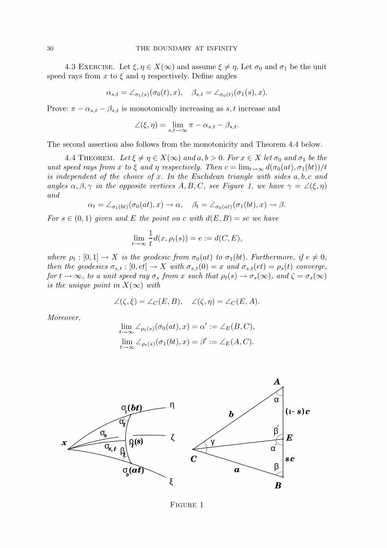
4.4 Theorem. Let ξ 6= η ∈ X(∞) and a, b > 0. For x ∈ X let σ0 and σ1 be theunit speed rays from x to ξ and η respectively. Then c = limt→∞ d(σ0(at), σ1(bt))/tis independent of the choice of x. In the Euclidean triangle with sides a, b, c andangles α, β, γ in the opposite vertices A,B,C, see Figure 1, we have γ = ∠(ξ, η)and

αt = ∠σ1(bt)(σ0(at), x) → α, βt = ∠σ0(at)(σ1(bt), x) → β.

For s ∈ (0, 1) given and E the point on c with d(E,B) = sc we have

limt→∞

1

td(x, ρt(s)) = e := d(C,E),

where ρt : [0, 1] → X is the geodesic from σ0(at) to σ1(bt). Furthermore, if e 6= 0,then the geodesics σs,t : [0, et] → X with σs,t(0) = x and σs,t(et) = ρs(t) converge,for t→ ∞, to a unit speed ray σs from x such that ρt(s) → σs(∞), and ζ = σs(∞)is the unique point in X(∞) with

∠(ζ, ξ) = ∠C(E,B), ∠(ζ, η) = ∠C(E,A).

Moreover,limt→∞

∠ρt(s)(σ0(at), x) = α′ := ∠E(B,C),

limt→∞

∠ρt(s)(σ1(bt), x) = β′ := ∠E(A,C).

x

η

ξ

ζσ

C

A

B

E

α

β

β

α

a

b(

s

)

σρt(s)

t)

1- s) c

γ

σ1(bt

αt

s

s, t βt

σ0(a

c

Figure 1


Proof. The independence of c from x is immediate from the definition ofasymptoticity. For γx = ∠x(ξ, η) and c(t) = L(σt) = d(σ0(at), σ1(bt)), we have

(a2 + b2 − 2ab cos γx)12 ≤ c(t)

t≤ a cosβt + b cosαt

= ct,E cos(αt − αt,E) = ct,E cos(βt − βt,E) ≤ ct,E

= (a2 + b2 − 2ab cos(π − αt − βt))12 ≤ (a2 + b2 − 2ab cos∠(ξ, η))

12 ,

where the inequalities in the first line follow from the Cosine Inequalities, see Propo-sition I.5.2, the equalities in the second line from Proposition I.5.3, where αt,E andβt,E are the angles and ct,E is the length of the third edge in the Euclidean trianglewith two edges of length a and b subtending an angle π−αt−βt, and the inequalityin the third line since

π − αt − βt ≤∠σ1(bt)(σ0(at), η) + ∠σ0(at)(σ1(bt), ξ)− π

≤∠σ0(at)(ξ, η) ≤ ∠(ξ, η).

Now c(t)/t tends to c and is independent of x. Since ∠(ξ, η) = supx∈X γx we get

c2 = a2 + b2 − 2ab cos∠(ξ, η)

and therefore ∠(ξ, η) = γ. Furthermore, we have π−αt−βt → ∠(ξ, η) and ct,E → cas t → ∞. Now c 6= 0 and hence αt,E → α, βt,E → β. We conclude that αt →α, βt → β as t→ ∞. We also have

d(x, ρt(s)) ≤ d(x, ρt(s)),

where ρt : [0, 1] → R2 is a line of length c(t) and where d(x, ρt(0)) = at, d(x, ρt(1)) =

bt. Now d(x, ρt(s))/t→ e as t→ ∞, therefore

lim supt→∞

1

td(x, ρt(s)) ≤ e.

On the other hand, we have

d2(x, ρt(s))

t2≥ a2 + s2

c(t)2

t2− 2as

c(t)

tcos(αt)

by the First Cosine Inequality. Since αt → α and c(t)/t→ c we conclude that

lim inft→∞

1

td(x, ρt(s)) ≥ e

and hence that d(x, ρt(s))/t→ e at t→ ∞.We now prove that the geodesics σs,t converge to a ray as claimed. Given

ε > 0, there is T ≥ 0 such that

|c(t)2

t2− c2|, |2asc(t)

tcosαt − 2asc cosα| < ε

2


for all t ≥ T . Then we obtain for t > t′ ≥ T and r = t′/t,

d2(σ0(at′), ρt(s))

t2≥ 1

t2(a2(t− t′)2 + s2c(t)2 − 2a(t− t′)sc(t) cosαt)

≥ a2(1 − r)2 + s2c2 − 2a(1 − r)sc cosα− ε.

Now denote by αt the angle in the Euclidean triangle with side lengths a, b, c(t)/tcorresponding to αt. Then αt ≥ αt and αt → α. By enlarging T if necessary, wealso have

|2asc(t)t

cosαt − 2asc cosα| < ε

2

for all t ≥ T . Since triangles in X are CAT0 we obtain, for t > t′ ≥ T ,

d2(σ0(at′), ρt(s))

t2≤ 1

t2(a2(t− t′)2 + s2c(t)2 − 2a(t− t′)sc(t) cosαt)

≤ a2(1 − r)2 + s2c2 − 2a(1 − r)sc cosα+ ε.

An analogous estimate holds for d(σ1(bt′), ρt(s)). Euclidean comparison for the

triangle (σ0(at′), σ1(bt

′), ρt(s)) shows that

d(ρ′t(s), ρt(s)) ≤ ((1 − r)e+ ε)t

for all t, t′ sufficiently large, where r = t′/t. On the other hand, d(x, ρt(s))/t → eand hence the triangle inequality implies

d(ρ′t(s), ρt(s)) ≥ ((1 − r)e− ε)t

for all t, t′ sufficiently large. In particular, up to the term εt (and ε can be chosen ar-bitrarily small), the concatenation of the geodesic from x to ρt′(s) with the geodesicfrom ρt′(s) to ρt(s) is a shortest connection from x to ρt(s). By comparison with Eu-clidean geometry we conclude that for any R ≥ 0, the distance d(σs,t(R), σs,t′(R))is arbitrarily small for all t, t′ sufficiently large. Hence the geodesic segments σs,tconverge to a ray σs. Note that σs has unit speed since d(x, ρt(s))/t→ e and thatρt(s) → σs(∞) = ζ by the very definition of the topology of X.

For t large, the triangle with vertices x, σ0(at), ρt(s) has sides of length ap-proximately equal to at, sct, et. By comparison we get

∠x(ξ, ζ) = limt→∞

∠x(σ0(at), ρt(s)) ≤ ∠C(B,E).

Similarly ∠x(η, ζ) ≤ ∠C(A,E). Clearly, ζ is independent of the choice of x andhence

(∗) ∠(ξ, ζ) ≤ ∠C(B,E), ∠(η, ζ) ≤ ∠C(A,E).

Now∠(ξ, ζ) + ∠(η, ζ) ≥ ∠(ξ, η) = ∠C(A,B),

hence we have equality in (∗).Suppose nowe that ζ ′ ∈ X(∞) is a point with

(∗∗) ∠(ξ, ζ ′) = ∠C(B,E), ∠(η, ζ ′) = ∠C(A,E),


and let σ′ be the unit speed ray from x to ζ ′. If ζ 6= ζ ′, then there is an ε > 0 suchthat d(σ′(et), ρt(s)) ≥ εt for all t sufficiently large. By comparison with Euclideangeometry we get that at least one of the following inequalities holds:

c20 = limt→∞

1

t2d2(σ0(at), σ

′(et)) ≥ s2c2 + ε2 or

c21 = limt→∞

1

t2d2(σ1(bt), σ

′(et)) ≥ (1 − s)2c2 + ε2.

However, by the first part of the proof we have

∠(ξ, ζ ′) =a2 + e2 − c20

2ae, ∠(η, ζ ′) =

b2 + e2 − c212be

.

Hence (∗∗) implies c20 = s2c2 and c21 = (1 − s)2c2. We conclude ζ = ζ ′.As for the last claim, let

α(t) = ∠ρt(s)(σ0(at), x), β(t) = ∠ρt(s)(x, σ1(bt)).

Then α(t) + β(t) ≥ π. By comparison with Euclidean geometry, applied to thetriangles ∆(ρt(s), x, σ0(at)) and ∆(ρt(s), x, σ1(bt)) we get

lim supt→∞

α(t) ≤ α′ and lim supt→∞

β(t) ≤ β′ .

Now α′ + β′ = π, hence the claim. �

4.5 Exercise. Use the notation of Theorem 4.4 and assume that e 6= 0. Let Fbe a point on the edge of length a on the Euclidean triangle such that d(C, F ) = rafor some r ∈ (0, 1). Prove:

d(E, F ) = limt→∞

1

td(ρt(s), σ0(rat))

and corresponding assertions about the angles at F .

4.6 Corollary. If ξ, η ∈ X(∞) are points with ∠(ξ, η) < π, then there is aunique minimizing geodesic in X(∞) (with respect to ∠) from ξ to η.

Proof. The existence of a geodesic from ζ to η follows from Proposition I.1.5and Theorem 4.4, where we put a = b = 0, s = 1/2. The uniqueness follows fromthe uniqueness of the point ζ in Theorem 4.4. �

The cone at infinity, C∞X , is the set [0,∞)×X(∞)/ ∼, where {0} ×X(∞)shrinks to one point, together with the metric d∞ defined by

(4.7) d∞((a, ξ), (b, η)) = a2 + b2 − 2ab cos∠(ξ, η).

That is, (C∞X, d∞) is the Euclidean cone over X(∞). We may also think of C∞Xas the set of equivalence classes of geodesic rays, where we do not require unit speedand where we say that geodesic rays σ0 and σ1 are equivalent if d(σ0(t), σ1(t)) isuniformly bounded in t. In the notation of Theorem 4.4 we have

d∞((a, ξ), (b, η)) = limt→∞

1

td(σ0(at), σ1(bt)).

In this sense, the geometry of X with respect to the rescaled metric d/t convergesto the geometry of C∞X as t→ ∞.

Given x ∈ X and a sequence of geodesics σn : [0, tn] → X with speed vn ≥ 0and σn(0) = x, we say that σn → (a, ξ) if tn → ∞, if vn → a and, if a 6= 0, ifσn(tn) → ξ.


Theorem 4.8. (C∞X, d∞) is a Hadamard space.

Proof. Note that C∞X is simply connected since we can contract C∞X ontothe distinguished point x∞ = [{0} ×X(∞)]. The metric d∞ is complete since ∠ isa complete metric on X(∞).

We show now that d∞ is a geodesic metric. To that end, let (a, ξ), (b, η) ∈C∞X . We want to show that there is a minimizing geodesic between these twopoints. The only non-trivial case is a, b > 0 and 0 < ∠(ξ, η) < π. Choose x ∈ Xand let σ0, σ1 be the unit speed rays from x with σ0(∞) = ξ and σ1(∞) = η. Then,in the notation of Theorem 4.4, the geodesics σs,t converge to geodesic rays σs ofspeed es > 0, 0 ≤ s ≤ 1, and, by Theorem 4.4 and the definition of d∞, the curveρ(s) = (es, σs(∞)), 0 ≤ s ≤ 1, is a minimizing geodesic form (a, ξ) to (b, η). It isimmediate from Corollary 4.6 (or Theorem 4.4) that ρ is the unique minimizinggeodesic from (a, ξ) to (b, η).

It remains to show that C∞X is nonpositively curved. By Lemma I.3.4, itsuffices to consider triangles in C∞X with minimizing sides. Let ∆ be such a triangleand let (ai, ξi), 1 ≤ i ≤ 3, be the vertices of ∆. The only non-trivial case is ai > 0and 0 < ∠(ξi, ξj) < π for i 6= j. Recall that the minimal geodesics ρi : [0, 1] → C∞Xfrom (ai, ξi) to (ai+1, ξi+1) are unique (indices are counted mod 3).

Let (e1, ζ1) = ρi(s1) and (e2, ζ2) = ρj(s2), where i 6= j and 0 < s1, s2 < 1. Letσ1 and σ2 be the unit speed rays from a given point x ∈ X to ζ1 and ζ2 respectively.By Theorem 4.4,

d∞((e1, ζ1), (e2, ζ2)) = limR→∞

1

Rd(σ1(e1R), σ2(e2R)).

Let σk be the unit speed ray from x to ξk, 1 ≤ k ≤ 3. If ρk,t : [0, 1] → X denotes thegeodesic from σk(akt) to σk+1(ak+1t) , and if σ1,t respectively σ2,t are the geodesicsfrom x with σ1,t(e1t) = ρi,t(s1) respectively σ2,t(e2t) = ρj,t(s2), then, by Theorem4.4,

σk(ekR) = limt→∞

σk,t(ekR), k = 1, 2.

For t large, the triangle (ρ1,t, ρ2,t, ρ3,t) has sides of length approximately tlk, wherelk = L(ρk). Now let (ρ1, ρ2, ρ3) be the Euclidean comparison triangle of (ρ1, ρ2, ρ3)and let dE = d(ρi(s1), ρj(s2)). Since X is a Hadamard space we conclude

d(ρi,t(s1), ρj,t(s2)) ≤ (dE + ε)t

where ε > 0 is given and t is sufficiently large. Hence

1

Rd(σ1(e1R), σ2(e2R)) = lim

t→∞

1

Rd(σ1,t(e1R), σ2,t(e2R))

≤ lim supt→∞

1

td(ρi,t(s1), ρj,t(s2)) ≤ dE .

It follows that triangles in C∞X are CAT0 and hence that C∞X is a Hadamardspace. �

4.9 Corollary. (X(∞),∠) has curvature ≤ 1. More precisely,(i) geodesics in X(∞) of length < π are minimal;(ii) triangles in X(∞) of perimeter < 2π are CAT1.

Proof. The relation between distances in C∞X and angles in X(∞) is ex-actly as the relation between distances in Euclidean space E3 and angles in theunit sphere S2. �


4.10 Lemma. Let X be a locally compact Hadamard space. In the notation ofTheorem 4.4 let a = b = 1 and assume that there is no geodesic in X from ξ to η.Let ρt(st) be the point on ρt closest to x. Then d(x, ρt(st)) → ∞. If ζ ∈ X(∞) isan accumulation point of ρt(st) for t→ ∞, then

∠(ξ, ζ) = ∠(ζ, η) = γ/2.

Proof. Since X is locally compact and since there is no geodesic from ξ to ηwe have d(x, ρt) → ∞ for t→ ∞. From Theorem 4.4 we conclude d(x, ρt(1/2))/t→cos(γ/2) < 1 and hence st 6= 0, 1. Therefore

∠ρt(st)(x, σ0(t)), ∠ρt(st)(x, σ1(t)) ≥ π/2.

Since (in the notation of Theorem 4.4) αt, βt → (π − γ)/2 we get

∠x(ξ, ζ), ∠x(ζ, η) ≤ γ/2.

The triangle inequality implies that we must have equality in these inequalities. �

Following Gromov, we denote by Td, the Tits metric, the interior metric onX(∞) associated to the angle metric ∠. The name derives from its close relation-ship with the Tits building associated to symmetric spaces. By definition, we haveTd(ξ, η) ≥ ∠(ξ, η) for all ξ, η ∈ X(∞).

4.11 Theorem. Assume that X is a locally compact Hadamard space. Theneach connected component of (X(∞), Td) is a complete geodesic space with curva-ture ≤ 1. Furthermore, for ξ, η ∈ X(∞) the following hold:(i) if there is no geodesic in X from ξ to η, then Td(ξ, η) = ∠(ξ, η) ≤ π;(ii) if ∠(ξ, η) < π, then there is no geodesic in X from ξ to η and there is a unique

minimizing Td-geodesic in X(∞) from ξ to η; Td-triangles in X of perimeter< 2π are CAT1;

(iii) if there is a geodesic σ in X from ξ to η, then Td(ξ, η) ≥ π, and equality holdsiff σ bounds a flat half plane;

(iv) if (ξn), (ηn) are sequences in X(∞) such that ξn → ξ and ηn → η in thestandard topology, then Td(ξ, η) ≤ lim infn→∞ Td(ξn, ηn).

Proof. The first assertion in (ii) and (iii) respectively is clear since ∠(ξ, η) =π if there is a geodesic in X from ξ to η. If there is no geodesic in X from ξ to η,then, by Lemma 4.10, there is a midpoint ζ in X(∞) between them with respect tothe ∠-metric. Now the ∠-metric on X(∞) is complete, see Proposition 4.1. Hencewe can construct an ∠-geodesic from ξ to η by choosing midpoints iteratively. Since∠-geodesics are Td-geodesics, we obtain (i). The uniqueness assertion in (ii) followsfrom the corresponding uniqueness assertion of midpoints in Theorem 4.4. Thecompleteness of Td also follows since the ∠-metric is complete, see Proposition 4.1.We now prove (iv) and that each connected component of (X(∞), Td) is geodesic.By the corresponding semicontinuity of ∠, see Proposition 4.1, we conclude from(i) that (iv) holds if lim infn→∞ Td(ξn, ηn) < π. From (ii) we also get that for anypair of points ξ, η ∈ X(∞) with Td(ξ, η) < π there is a minimizing Td-geodesicfrom ξ to η. By induction we assume that this also holds when we replace π bykπ, k ≥ 1. Now suppose lim infn→∞ Td(ξn, ηn) < (k + 1)π. By th definition of Td,


there is a point ζn almost half way between ξn and ηn. Passing to a subsequence ifnecessary, we assume ζn → ζ in the standard topology and obtain, by induction,

Td(ξ, η) ≤ Td(ξ, ζ) + Td(ζ, η)

≤ lim infn→∞

Td(ξn, ζn) + lim infn→∞

Td(ζn, ηn) ≤ lim infn→∞

Td(ξn, ηn).

In particular, Td(ξ, η) < (k + 1)π. There exists (another) sequence (ζn) such that

Td(ξ, ζn), Td(η, ζn) → Td(ξ, η)/2,

hence, by the semicontinuity, there is a point ζ with

Td(ξ, ζ) = Td(η, ζ) = Td(ξ, η)/2.

By the inductive hypothesis, there are minimizing Td-geodesics from ξ to ζ and ζ toη. Their concatenation is a minimizing Td-geodesic from ξ to η. Hence we conclude(iv) and that the components of (X(∞), Td) are geodesic spaces.

As for the statement about flat half planes in (iii), let ζ be a point withTd(ζ, ξ) = Td(ζ, η) = π/2. Since

∠x(ζ, ξ) + ∠x(ζ, η) ≥ π

for any x on the geodesic (in X) from ξ to η and ∠x ≤ Td, we have

∠x(ζ, ξ) = ∠x(ζ, η) = π/2

for all such x. Now the rigidity part of Lemma I.5.8(i) applies.The claims about the curvature bound and about triangles in (ii) are imme-

diate from Corollary 4.9. �

THE DUALITY CONDITION 37

CHAPTER III

WEAK HYPERBOLICITY

One of our main objectives in this chapter is the discussion of transitivityproperties of the geodesic flow and related topics. The first two sections are greatlyinfluenced by the work of Eberlein on geodesic flows in [Eb2, Eb3]. The thirdsection deals with the main results of the author’s thesis (published in [Ba1]),but here in the context of Hadamard spaces instead of Hadamard manifolds. Thefourth section deals with applications to harmonic functions and random walks oncountable groups, compare [Ba3, BaL1]. Many of the ideas in Section 4 go back toFurstenberg [Fu1, Fu2, Fu3].

Let X be a Hadamard space. We say that X is geodesically complete if everygeodesic segment of X is part of a complete geodesic of X , that is, a geodesic whichis defined on the whole real line. For X geodesically complete, we denote by GX theset of unit speed geodesics of X , equipped with the topology of uniform convergenceon bounded subsets. The geodesic flow (gt) acts on GX by reparameterization,

gt(σ)(s) = σ(s+ t) .

If X is a smooth manifold, then

GX → SX ; σ → σ(0)

defines a homeomorphism from GX to the unit tangent bundle SX of X . Withrespect to this homeomorphism, the geodesic flow above corresponds to the usualgeodesic flow on SX (also denoted gt),

gt(v) = γv(t), v ∈ SX,

where γv denotes the geodesic in X with γv(0) = v.

1. The duality condition

In our considerations it will be important to have a large group of isometries.Let X be a Hadamard space and Γ a group of isometries of X . Following Eberlein[Eb2], we say that ξ, η ∈ X(∞) are Γ-dual if there is a sequence (ϕn) in Γ suchthat ϕn(x) → ξ and ϕ−1

n (x) → η as n → ∞ for some (and hence any) x ∈ X .Duality is a symmetric relation. The set of points Γ-dual to a given point in X(∞)is closed and Γ-invariant. We say that Γ satisfies the duality condition if for anyunit speed geodesic σ : R → X the endpoints σ(−∞) and σ(∞) are Γ-dual. Theduality condition was introduced by Chen and Eberlein [CE1]. The condition issomewhat mysterious, at least as far as Hadamard spaces are concerned (as opposedto Hadamard manifolds). May be it is only reasonable for geodesically completeHadamard spaces.

Typeset by AMS-TEX

38 WEAK HYPERBOLICITY

1.1 Lemma [Eb2]. Let X be a geodesically complete Hadamard space, and letσ, ρ : R → X be unit speed geodesics in X. Let (ϕn) be a sequence of isometries ofX such that ϕ−1

n (x) → σ(∞) and ϕn(x) → ρ(−∞) as n→ ∞ for some (and henceany) x ∈ X. Then there are sequences (σn) in GX and (tn) in R such that σn → σ,tn → ∞ and ϕn ◦ gtn(σn) → ρ as n→ ∞.

1.2 Remarks. (a) The converse to Lemma 1.1 is clear: let σ, ρ ∈ GX andsuppose there are sequences (σn) in GX , (tn) in R and (ϕn) of isometries of X suchthat σn → σ, tn → ∞ and ϕn ◦ gtn(σn) → σ as n→ ∞. Then ϕ−1

n (x) → σ(∞) andϕn(x) → ρ(−∞) as n→ ∞ for one (and hence any) x ∈ X .

(b) Note that the assumption on the sequence (ϕn) in Lemma 1.1 only specifiesσ(∞) and ρ(−∞). Thus we may replace σ by any asymptotic σ′ ∈ GX and ρ byany negatively asymptotic ρ′ ∈ GX , keeping the sequence (ϕn) fixed.

Since σn → σ and ϕ−1n ◦ gtn(σn) → ρ we have

tn − d(σ(0), ϕ−1n (ρ(0))) → 0 as n→ ∞ .

For σ′ asymptotic to σ we also have

d(σ′(0), ϕ−1n (ρ(0)))− d(σ(0), ϕ−1

n (ρ(0))) → b(σ(∞), σ(0), σ′(0))

as n→ ∞. Hence we may replace the sequence (tn) by the sequence (t′n) given by

t′n = tn + b(σ(∞), σ(0), σ′(0)), n ∈ N ,

when replacing σ by σ′. A similar remark applies to geodesics ρ′ ∈ GX negativelyasymptotic to ρ.

Proof of Lemma 1.1. For m ≥ 0 and n ∈ N let σn,m : R → X be a unitspeed geodesic with

σn,m(−m) = σ(−m) and σn,m(tn,m +m) = ϕ−1n (ρ(m)) ,

wheretn,m = d(σ(−m), ϕ−1

n (ρ(m)))− 2m.

Set N(0) = 1 and define N(m), m ≥ 1, recursively to be the smallest number> N(m− 1) such that

d(σn,m(m), σ(m)) ≤ 1

mand d(ϕn ◦ σn,m(tn,m −m), ρ(−m)) ≤ 1

m

for all n ≥ N(m). Note that such a number N(m) exists since ϕ−1n (ρ(m)) → σ(∞)

and ϕn(σ(−m)) → ρ(−∞). Now set σn := σn,N(m) for N(m) ≤ n < N(m+ 1). �

1.3 Corollary. Let X be a geodesically complete Hadamard space and Γ agroup of isometries of X satisfying the duality condition. Let σ, ρ : R → X be unitspeed geodesics in X with σ(∞) = ρ(∞). Then there are sequences (σn) in GX,(tn) in R and (ϕn) in Γ such that σn → σ, tn → ∞ and ϕn ◦ gtn(σn) → ρ asn→ ∞.

Proof. Since Γ satisfies the duality condition, there is a sequence (ψn) ofisometries in Γ such that ψn(x) → ρ(∞) and ψ−1

n (x) → ρ(−∞) as n → ∞. Nowσ(∞) = ρ(∞), and hence Lemma 1.1 applies. �

THE DUALITY CONDITION 39

We say that a geodesic σ ∈ GX is nonwandering mod Γ (with respect to thegeodesic flow) if there are sequences (σn) in GX , (tn) in R and (ϕn) in Γ suchthat σn → σ, tn → ∞ and ϕn ◦ gtn(σn) → σ. The set of geodesics in GX that arenonwandering mod Γ is closed in GX and invariant under the geodesic flow and Γ.It is clear that the endpoints of a geodesic σ ∈ GX are Γ-dual if σ is nonwanderingmod Γ. Vice versa, Lemma 1.1, applied in the case where X is geodesically completeand σ = ρ, shows that a geodesic σ ∈ GX is nonwandering mod Γ if the endpointsof σ are Γ-dual.

1.4 Corollary. Let X be a geodesically complete Hadamard space and Γ agroup of isometries of X. Then Γ satisfies the duality condition if and only if everyσ ∈ GX is nonwandering mod Γ. �

We say that a geodesic σ ∈ GX is Γ-recurrent if there exist sequences (tn) inR and (ϕn) in Γ such that tn → ∞ and ϕn ◦ gtn(σ) → σ as n → ∞. The set ofΓ-recurrent geodesics in GX is invariant under the geodesic flow and Γ.

1.5 Corollary. Let X be a geodesically complete, separable Hadamard spaceand Γ a group of isometries of X. Then Γ satisfies the duality condition if and onlyif a dense set of geodesics σ ∈ GX is Γ-recurrent.

Proof. Since X is separable, the topology of X ,and hence also of GX , has acountable base. Now Corollary 1.4 implies that the set of Γ-recurrent geodesics isa dense Gδ-subset of GX if Γ satisfies the duality condition. The other direction isclear. �

If X is a Hadamard manifold, then the Liouville measure on SX is invariantunder the geodesic flow. Hence, if Γ is a group of isometries of X that acts properlydiscontinuously and such that vol(X/Γ) < ∞, then Γ satisfies the duality condi-tion by the Poincare recurrence theorem and Corollary 1.4. However, for a generalHadamard space X , there is (so far) no natural invariant measure on GX with goodproperties.

1.6 Question. Let X be a geodesically complete Hadamard space and Γ agroup of isometries of X . Does Γ satisfy the duality condition if it acts properlydiscontinuously and cocompactly?

1.7 Problem/Exercise. LetX be a geodesically complete Hadamard space.Construct measures on GX which are invariant under isometries and the geodesicflow of X .

In the case of 2-dimensional polyhedra with piecewise smooth metrics, theanswer to Question 1.6 is affirmative, see [BB3]. In this reference, one also findsa natural generalization of the Liouville measure for geodesic flows on polyhedrawith piecewise smooth metrics.

The following lemma and proposition are taken from [CE1] and [BBE] respec-tively.

1.8 Lemma. Suppose ξ, η ∈ X(∞) are the endpoints of a geodesic σ : R → X.Let (ϕn) be a sequence of isometries of X such that ϕn(x) → ξ and ϕ−1

n (x) → ζ ∈X(∞) as n→ ∞. Then ϕ−1

n (η) → ζ as n→ ∞.

Proof. Let x = σ(0). Then ∠x(ξ, ϕn(x)) → 0 and hence

∠x(ϕn(x), η) ≥ π − ∠x(ξ, ϕn(x)) → π .


By comparison with Euclidean geometry we get, for the metric dx,R as in (II.2.3),

dx,R(ϕ−1n (x), ϕ−1

n (η)) = dϕn(x),R(x, η) → 0 ,

where R > 0 is arbitrary. Since ϕ−1n (x) → ζ we conclude ϕ−1

n (η) → ζ. �

1.9 Proposition. Suppose X is geodesically complete and Γ satisfies the du-ality condition. Let ξ ∈ X(∞). Then Γ operates minimally on the closure Γ(ξ) of

the Γ-orbit of ξ, that is, Γ(ζ) = Γ(ξ) for any ζ ∈ Γ(ξ).

Proof. It suffices to show that ξ ∈ Γ(ζ) for any ζ ∈ Γ(ξ). Since X is geodesi-cally complete, there are geodesics σ, ρ : R → X with σ(∞) = ξ and ρ(∞) = ζ. Letξ′ = σ(−∞) and ζ ′ = ρ(−∞).

Since Γ satisfies the duality condition, ξ′ is Γ-dual to ξ and ζ ′ is Γ-dual toζ. Now ζ is Γ-dual to ξ′ because the set of points Γ-dual to ξ′ is Γ-invariant andclosed. By Lemma 1.8 this implies that ξ′ ∈ Γ(ζ ′).

Choose a sequence (ϕn) in Γ with ϕn(ζ′) → ξ′. Form > 0, let σm be a complete

geodesic with σm(0) = σ(m) and σm(−∞) = ϕn(ζ ′), where n = n(m) ≥ m ischosen so large that d(σm, σ(0)) ≤ 1. Then σm(∞) → ξ and σm(−∞) is Γ-dual toσm(∞). Therefore σm(∞) is Γ-dual to ζ ′ = ϕ−1

n (σm(−∞)). Hence ζ ′ is Γ-dual to

ξ = limm→∞ σm(∞). Now Lemma 1.8 implies ξ ∈ Γ(ζ). �

1.10 Remark. The duality condition has other useful technical properties.(1) Let X1 and X2 be Hadamard spaces with metrics d1 and d2 respectively

and let X be the Hadamard space X1 ×X2 with the metric d =√d21 + d2

2. If Γ isa group of isometries of X satisfying the duality condition such that any ϕ ∈ Γ isof the form ϕ = (ϕ1, ϕ2), where ϕi is an isometry of Xi, i = 1, 2, then

Γ1 := {ϕ1 | there is an isometry ϕ2 of X2 with (ϕ1, ϕ2) ∈ Γ}

and the corresponding group Γ2 satisfy the duality condition. This is clear sincegeodesics in X are pairs (σ1, σ2), where σ1 is a geodesic of X1 and σ2 is a geodesicof X2. See [Eb10,16] for applications of this property in the case of Hadamardmanifolds.

Note that Γ1 and/or Γ2 need not act properly discontinuously even if Γ does.Thus a condition like cocompactness + proper discontinuity does not share theabove property of the duality condition.

(2) Clearly the duality condition passes from a group Γ of isometries of aHadamard space X to a larger group of isometries of X . Vice versa, if X is geodesi-cally complete and separable and if ∆ is a subgroup of finite index in Γ, then ∆satisfies the duality condition if Γ does [Eb10]. To see this, let σ ∈ GX be a Γ-recurrent geodesic. Choose sequences (tn) in R and (ϕn) in Γ such that tn → ∞and ϕn ◦ gtn(σ) → σ. Now ∆ has finite index in Γ. Hence we may assume, afterpassing to a subsequence, that ϕn = ψnϕ, where ϕ ∈ Γ is fixed and ψn ∈ ∆ for alln ∈ N. Then

σ′n = ϕn ◦ gtn(σ) → σ

andσm,n = (ψmψ

−1n ) ◦ gtm−tn(σ′

n) = ϕm ◦ gtm(σ) → σ .

Choose m = m(n) convenient to get that σm(n),n → σ. This shows that σ isnonwandering mod ∆. Now the set of geodesics in GX which are nonwandering

GEODESIC FLOWS ON HADAMARD SPACES 41

mod ∆ is closed, and the set of Γ-recurrent geodesics in GX is dense in GX , seeCorollary 1.4. Hence ∆ satisfies the duality condition.

We come back to the beginning of this section. We said there that we willbe in need of a large group of isometries, and we made this precise by introducingthe duality condition. One might think that the isometry group of a homogeneousHadamard manifold X is large; however, it is not in our sense, except if X is asymmetric space (see [Eb10], Proposition 4.9).

1.11 Definition/Exercise/Question. Let X be a Hadamard space and Γa group of isometries of X . The limit set L(Γ) ⊂ X(∞) of Γ is defined to be theset of all ξ ∈ X(∞) such that there is a sequence (ϕn) in Γ with limn→∞ ϕn(x) = ξfor one (and hence any) x ∈ X . Show L(Γ) = X(∞)

(i) if there is a bounded subset B in X with ∪ϕ∈Γϕ(B) = X or(ii) if X is geodesically complete and Γ satisfies the duality condition.

In many results below we assume that X is geodesically complete and that Γ sat-isfies the duality condition. Can one (you) replace the duality condition by theassumption L(Γ) = X(∞).

2. Geodesic flows on Hadamard spaces

2.1 Definition. Let X be a geodesically complete Hadamard space and Γ agroup of isometries of X . We say the geodesic flow of X is topologically transitivemod Γ if for any two open non-empty subsets U, V in GX there is t ∈ R and ϕ ∈ Γsuch that gt(U) ∩ ϕ(V ) 6= ∅.

2.2 Remark. If X is separable, then the topology of X , and therefore thetopology of GX , has a countable base. Hence the geodesic flow is topologicallytransitive mod Γ if and only if it has a dense orbit mod Γ: there is a σ in GX suchthat for any σ′ in GX there are sequences (tn) in R and ϕn in Γ with ϕng

tnσ → σ′.

After all our preparations we are ready for the following result from [Eb3].

2.3 Theorem. Let X be a geodesically complete, separable Hadamard space,and let Γ be a group of isometries of X satisfying the duality condition. Then thefollowing are equivalent:(i) gt is topologically transitive mod Γ;(ii) for some ξ ∈ X(∞), the orbit Γ(ξ) is dense in X(∞);(iii) for every ξ ∈ X(∞), the orbit Γ(ξ) is dense in X(∞);(iv) X(∞) does not contain a non-empty Γ-invariant proper closed subset.

Proof. Clearly (iii) ⇔ (iv) and (iii) ⇒ (ii). The implication (i) ⇒ (ii) isimmediate from Remark 2.2 above. The implication (ii) ⇒ (iii) follows from Propo-sition 1.9. It remains to prove (ii) ⇒ (i).

We let U(∞) respectively V (∞) be the set of points σ(∞) in X(∞) withσ ∈ U respectively V . Then U(∞) and V (∞) are open and non-empty. Applying(ii) we can assume U(∞) ⊂ V (∞). Let σ ∈ U . Then there is a geodesic ρ ∈ V withρ(∞) = σ(∞). Now Corollary 1.3 applies. �

2.4 Theorem. Let X be a geodesically complete and locally compact Hada-mard space, and let Γ be a group of isometries of X satisfying the duality condition.Then the following are equivalent:


(i) the geodesic flow (gt) of X is not topologically transitive mod Γ;(ii) X(∞) contains a non-empty Γ-invariant proper compact subset;(iii) the geodesic flow (gt) of X admits a non-constant Γ-invariant continuous first

integral f : GX → R such that f(σ) = f(ρ) for all σ, ρ ∈ GX with σ(∞) =ρ(∞) or σ(−∞) = ρ(−∞).

Each of these conditions implies that every geodesic of X is contained in a flatplane, that is, a convex subset of X isometric to the Euclidean plane.

Proof. X is separable because X is locally compact. Hence (i) ⇔ (ii) byTheorem 2.3. The implication (iii) ⇒ (ii) is clear since we assume the integral to becontinuous, non-constant and Γ-invariant and since X(∞) is compact. It remainsto show (ii) ⇒ (iii) and the existence of the flat planes.

To that end, let C ⊂ X(∞) be a non-empty Γ-invariant proper compactsubset. For σ ∈ GX we set

(2.5) f(σ) = minζ∈C

∠σ(0)(σ(∞), ζ) .

We claim that the function f is an integral of the geodesic flow as asserted. Notethat f is Γ-invariant since C is.

The continuity of angle measurement at a fixed point, see I.3.x, implies thatfor any σ ∈ GX there is ζ ∈ C with f(σ) = ∠σ(0)(σ(∞), ζ). Obviously, or by

Proposition II.4.2, we have that f(gt(σ)) is monotonically not decreasing in t.Suppose first that σ ∈ GX is Γ-recurrent. Choose sequences (tn) in R and

(ϕn) in Γ such that tn → ∞ and ϕn ◦ gtn(σ) → σ. By the Γ-invariance of f and themonotonicity we have

f(ϕn ◦ gtn(σ)) = f(gtn(σ)) ≥ f(σ) .

The semicontinuity of angle measurement, see I.3.x, implies

lim infn→∞

f(ϕn ◦ gtn(σ)) ≤ f(σ) .

We conclude that f(gt(σ) = f(σ) for all t ≥ 0, and hence for all t ∈ R since gs(σ)is Γ-recurrent for all s ∈ R. We also conclude that there is a point ζ(σ) ∈ C suchthat

f(gt(σ)) = ∠σ(t)(σ(∞), ζ(σ)) = ∠(σ(∞), ζ(σ)) = minζ∈C

∠(σ(∞), ζ) .

In particular, σ bounds a flat half plane Hσ with ζ(σ) ∈ Hσ(∞) if σ(∞) 6∈ C.Now let σ ∈ GX be arbitrary. Let (σn) be a sequence of Γ-recurrent unit

speed geodesics converging to σ. Passing to a subsequence if necessary, the corre-sponding half planes Hσn

and points ζ(σn) converge to a flat half plane Hσ alongσ respectively a point ζ(σ) ∈ Hσ(∞). We conclude

f(σ) = limn→∞

f(σn) = ∠(σ(∞), ζ(σ)) .

Therefore f is continuous; now Lemma 1.1 implies that f(σ) = f(ρ) if σ(∞) = ρ(∞)respectively if σ(−∞) = ρ(−∞); f is non-constant since C is proper.

THE FLAT HALF PLANE CONDITION 43

Let σ ∈ GX and let Hσ, ζ(σ) be as above. Let ρt : R → X be a unit speedgeodesic with ρt(0) = σ(t) and ρt(∞) = ζ(σ). For s ∈ R, let σs : R → X be a unitspeed geodesic σs(t) = ρt(s) and σs(∞) = σ(∞). Then clearly

f(σ) = f(σs) = ∠σs(t)(ζ(σ), σs(∞)) .

Therefore ρt|[s,∞) and σs|[t,∞) span a flat cone Cs,t. This cone contains σ([t,∞)) ifs < 0. NowX is locally compact. Hence we obtain a flat plane containing σ as a limitof the cones Csn,tn for some appropriate sequences sn → −∞ and tn → −∞. �

2.6 Problem. Suppose X is geodesically complete and irreducible with agroup Γ of isometries satisfying the duality condition. Assume furthermore thatevery geodesic of X is contained in a flat plane. Claim: X is a symmetric space ora Euclidean building.

This is known in the smooth case, which excludes the case of Euclidean build-ings. In Chapter IV we will discuss the proof. In the singular case, if dimX = nand every geodesic of X is contained in an n-flat, that is, a convex subset of Xisometric to n-dimensional Euclidean space, then X is a Euclidean building [Kl].

3. The flat half plane condition

In this section we assume that X is a locally compact Hadamard space. Then,if σ : R → X is a geodesic which does not bound a flat half plane, there is a constantR > 0 such that σ does not bound a flat strip of width R.

3.1 Lemma. Let σ : R → X be a unit speed geodesic which does not bounda flat strip of width R > 0. Then there are neighborhoods U of σ(−∞) and V ofσ(∞) in X such that for any ξ ∈ U and η ∈ V there is a geodesic from ξ to η, andfor any such geodesic σ′ we have d(σ′, σ(0)) < R. In particular, σ′ does not bounda flat strip of width 2R.

Proof. If the assertion of the lemma does not hold, then there are sequences(xn) and (yn) in X with xn → σ(−∞) and yn → σ(∞) such that the unit speedgeodesic segment σn from xn to yn, parameterized such that σn(0) is the point onσn closest to z := σ(0), satisfies d(σn(0), z) ≥ R for all n ∈ N. Let zn be the pointon the geodesic from z to σn(0) with d(z, zn) = R. By the choice of σn(0),

∠σn(0)(z, xn), ∠σn(0)(z, yn) ≥π

2.

Hence also∠zn

(z, xn), ∠zn(z, yn) ≥

π

2.

Passing to a subsequence if necessary we assume zn → z∞. Then d(z, z∞) = R and

∠z∞(z, σ(−∞)), ∠z∞(z, σ(∞)) ≥ π

2.

We also have∠z(σ(−∞), z∞) + ∠z(σ(∞), z∞) ≥ π .

Applying Proposition I.5.8(i) we conclude

∠z(σ(−∞), z∞) = ∠z∞(σ(−∞), z) = ∠z(σ(∞), z∞) = ∠z∞(σ(∞), z) =π

2.


Hence the unit speed rays ω− respectively ω+ from z∞ to σ(−∞) and σ(∞) re-spectively span flat half strips with σ|(−∞, 0] respectively σ|[0,∞), see PropositionI.5.8(i). In particular, σ(−t) respectively σ(t) is the point on σ closest to ω−(t) re-spectively ω+(t), t > 0. Hence d(ω−(t), ω+(t)) ≥ 2t, and hence ω− and ω+ combineto give a geodesic ω from σ(−∞) to σ(∞) through z∞. Therefore ω is parallel toσ and ω and σ span a flat strip of width R. This is a contradiction. �

3.2 Lemma. Let σ : R → X be a unit speed geodesic which does not bound aflat half plane. Let (ϕn) be a sequence of isometries of X such that ϕn(x) → σ(∞)and ϕ−1

n (x) → σ(−∞) for one (and hence any) x ∈ X. Then for n sufficientlylarge, ϕn has an axis σn such that σn(∞) → σ(∞), σn(−∞) → σ(−∞) as n→ ∞.

Proof. There is an R > 0 such that σ does not bound a flat strip of widthR. Let x = σ(0) and choose ε > 0, r > 0 such that

U = U(x, σ(−∞), r, ε) and V = U(x, σ(∞), r, ε).

are neighborhoods as in Lemma 3.1. By comparison with Euclidean geometry wefind that there is an R′ > r such that for any y ∈ X we have

(∗)d(σ(r), σx,y(r)) < ε or d(σ(−r), σx,y(r)) < ε

if d(y, σ) ≤ R and d(y, x) ≥ R′.

By the definition of U and V this means that y ∈ U ∪ V if d(y, σ) ≤ R andd(y, x) ≥ R′.

Assume that ϕn, for any n in a subsequence, fixes a point xn ∈ X outsideU ∪ V with d(x, xn) ≥ 2R′. Let σn = σx,xn

be the unit speed geodesic (or ray re-spectively if xn ∈ X(∞)) from x to xn. Then the displacement function d(ϕn(z), z)is monotonically decreasing along σn. Let yn = σn(R′) and y′n = σn(2R

′). Then

∠yn(y′n, ϕn(yn))+∠yn

(y′n, ϕ−1n (yn)) =

∠yn(y′n, ϕn(yn))+∠ϕn(yn)(ϕn(y′n), yn) ≤ π

since

d(yn, ϕn(yn)) = d(yn, ϕ−1n (yn)) ≥ d(y′n, ϕn(y

′n)) = d(y′n, ϕ

−1n (y′n))

(consider the quadrangle spanned by yn, y′n, ϕn(yn), ϕn(y

′n)). Now

∠yn(y′n, ϕ

±1n (yn)) + ∠yn

(x, ϕ±1n (yn)) ≥ ∠yn

(y′n, x) = π

and therefore

(∗∗) ∠yn(x, ϕn(yn)) + ∠yn

(x, ϕ−1n (y′n)) ≥ π.

We also haved(ϕ±1

n (yn), ϕ±1n (x)) = d(yn, x) = R′,

and hence ϕn(yn) → σ(∞) and ϕ−1n (yn) → σ(−∞) (for the given subsequence).

After passing to a further subsequence if necessary, we can assume yn → y. Thend(y, σ) ≥ R by (∗) since y 6∈ U ∪ V and d(y, x) = R′. By (∗∗), the rays from yto σ(−∞) respectively σ(∞) combine to give a geodesic parallel to σ. Thereforeσ bounds a flat strip of width R, a contradiction. Hence we obtain that, for nsufficiently large, any fixed point of ϕn is contained in U ∪ V ∪B(x, 2R′).

Using Lemma 3.1 it is now easy to exclude that ϕn is elliptic or parabolic(for this compare Proposition II.3.4) for all n sufficiently large. For large n, theendpoints of an axis σn of ϕn have to be in U ∪ V by what we said above. It isclear from Lemma 3.1 that not both endpoints of σn are in one of the sets, U orV . Hence the lemma. �

THE FLAT HALF PLANE CONDITION 45

3.3 Lemma. Let ϕ be an isometry of X with an axis σ : R → X, where σ isa unit speed geodesic which does not bound a flat half plane. Then(i) for any neighborhood U of σ(−∞) and any neighborhood V of σ(∞) in X

there exists N ∈ N such that

ϕn(X \ U) ⊂ V, ϕ−n(X \ V ) ⊂ U for all n ≥ N ;

(ii) for any ξ ∈ X(∞) \ {σ(∞)} there is a geodesic σξ from ξ to σ(∞), and anysuch geodesic does not bound a flat half plane. For K ⊂ X(∞) \ {σ(∞)}compact, the set of these geodesics is compact (modulo parameterization).

Proof. Let x = σ(0). We can assume that

U = U(x, σ(−∞), R, ε) and V = U(x, σ(∞), R, ε).

By comparison with Euclidean geometry we find that

(∗) ϕ−1(U) ⊂ U and ϕ(V ) ⊂ V .

If (i) is not true, there is a sequence nk → ∞ and, say, a sequence (xk) in X \ Usuch that ϕnk(xk) 6∈ V . Passing to a subsequence, we may assume xk → ξ ∈ X \U .From (∗) we conclude ϕm(xk) 6∈ V for 0 ≤ m ≤ nk, and hence we get

(∗∗) ϕm(ξ) 6∈ V for all m ≥ 0.

In particular, ξ ∈ X(∞). Now the set K of all ξ ∈ X(∞) \ U satisfying (∗∗) iscompact and invariant under ϕm, m ≥ 1. By our assumption K 6= ∅. Now chooseξ ∈ K such that ∠σ(0)(σ(∞), ξ) is minimal. Since ϕ(σ(∞)) = σ(∞),

∠σ(0)(σ(∞), ϕm(ξ)) ≤ ∠σ(ma)(σ(∞), ϕm(ξ)) = ∠σ(0)(σ(∞), ξ),

where a > 0 is the period of ϕ. By the choice of ξ we conclude

∠σ(0)(σ(∞), ϕm(ξ)) = ∠σ(ma)(σ(∞), ϕm(ξ)),

hence the rays from σ(0) and σ(ma) to ϕm(ξ) together with σ|[0, ma] bound aflat convex region. Since m is arbitrary and since ϕ shifts σ, we conclude that σbounds a flat half plane, a contradiction. Thus (i) follows. Now (ii) is an immediateconsequence of (i) and Lemma 3.1. �

Let Γ be a group of isometries of the Hadamard space X . We say that anon-constant geodesic σ in X is Γ-closed if it is an axis of an axial isometry ϕ ∈ Γ.

3.4 Theorem. Assume that X is a locally compact Hadamard space contain-ing a unit speed geodesic σ : R → X which does not bound a flat half plane and thatΓ is a group of isometries of X satisfying the duality condition. Then we have:

If X(∞) contains at least three points, then X(∞) is a perfect set: for anyξ ∈ X(∞), there is a sequence (ξn) in X(∞) \ {ξ} such that ξn → ξ. Furthermore,for any two non-empty open subsets U, V of X(∞) there is a ϕ ∈ Γ with

ϕ(X(∞) \ U) ⊂ V, ϕ−1(X(∞) \ V ) ⊂ U.


More precisely, there is a Γ-closed geodesic σ with σ(−∞) ∈ U and σ(∞) ∈ V suchthat σ does not bound a flat half plane.

Proof. By Lemma 3.2, there is an isometry ϕ0 in Γ with an axis σ0 whichdoes not bound a flat half plane. Since X(∞) contains more than two points, thereis a point ξ ∈ X(∞) \ {σ0(±∞)}. By Lemma 3.3, ϕ±n

0 (ξ) → σ0(±∞), hence thefirst assertion holds for σ0(±∞). Again by Lemma 3.3, there is a geodesic σ1 fromσ0(−∞) to ξ and this geodesic does not bound a flat half plane. By Lemma 3.2,any two neighborhoods of the endpoints of σ1 contain endpoints of an axis σ′

1 ofan isometry ϕ1 in Γ and σ′

1 does not bound a flat half plane. Then a sufficient highpower of ϕ1 maps σ0(+∞) into the given neighborhood, hence the first assertionalso holds for ξ.

If U, V are non-empty and open in X(∞), there is, by the first step, a pointξ ∈ U − σ0(∞). By Lemma 3.3, there is a geodesic half plane. By Lemma 3.2 thereis a Γ-closed geodesic σ2 with σ2(−∞) ∈ U such that σ2 does not bound a flat halfplane. Again by the first part, there is a point η ∈ V − σ2(−∞) and, by Lemma3.3, a geodesic σ3 from σ2(−∞) to η which does not bound a flat half plane. ByLemma 3.2, there is a Γ-closed geodesic σ as claimed. �

3.5 Theorem. Let X and Γ be as in Theorem 3.4. Suppose X(∞) containsat least three points.(i) If X is geodesically complete, then the geodesic flow is topologically transitive

mod Γ.(ii) Γ contains free non-abelian subgroups.

Proof. (i) This is immediate from Theorem 2.4. Alternatively we can argueas follows: Theorem 3.4 and Lemma 3.3 imply that the Γ-orbit of any point ξ ∈X(∞) is dense in X(∞). Hence the geodesic flow of X is topologically transitivemod Γ by Theorem 2.3.

(ii) By the first assertion of Theorem 3.4, X(∞) contains non-empty opensubsets W1,W2 with

(∗) W1 ∩W2 = ∅ and W1 ∪W2 6= X(∞).

By the second assertion of Theorem 3.4 and Lemma 3.3, Γ contains isometriesϕ1, ϕ2 with axis σ1, σ2 which do not bound flat half planes such that σi(±∞) ∈Wi

and

(∗∗) ϕ±ki (X(∞) \Wi) ⊂Wi, i = 1, 2 ,

for all k 6= 0. Let ξ ∈ X(∞) \ (W1 ∪ W2). It follows from (∗) and (∗∗) that anon-trivial word w in ϕ1 and ϕ2, considered as an element of Γ, maps ξ to Wi ifϕi is the first letter of w, i = 1, 2. Hence w(ξ) 6= ξ and therefore w 6= id. It followsthat ϕ1 and ϕ2 generate a free subgroup of Γ. �

3.6 Remark. If X is a Hadamard manifold with a unit speed geodesic σ :R → X which does not bound a flat half plane, and if Γ is a group of isometriesof X satisfying the duality condition, then the geodesic flow of X is topologicallymixing mod Γ [Ba1]: for any two non-empty open subsets U, V in GX there is aT ≥ 0 such that for any t ≥ T there is ϕ ∈ Γ with gt(U)∩ϕ(V ) 6= ∅. This does nothold in the general case we consider, even if we impose the strongest hyperbolicity

HARMONIC FUNCTIONS AND RANDOM WALKS 47

assumption. For example, if X is the tree with all vertices of valence three and alledges of length one, and if U respectively V is the set of all σ ∈ GX such that σ(0)is ε-close to a vertex respectively the midpoint of an edge, where ε < 1/4, thengt(U)∩ϕ(V ) = ∅ for all t ∈ Z and every isometry ϕ of X . It is, however, possible tostrengthen the above result about topological transitivity and to obtain a propertyintermediate between it and topological mixing.

In Chapter IV we prove that a Hadamard manifold M with a group Γ ofisometries satisfying the duality condition contains a unit speed geodesic whichdoes not bound a flat half plane if and only if it contains a unit speed geodesicσ which does not bound an infinitesimal flat half plane. By the latter we meanthat there is no parallel vector field V along σ such that ‖V ‖ = 1, V ⊥ σ andK(σ ∧ V ) ≡ 0. It is easy to see that σ satisfies this condition if and only if σ ishyperbolic in the sense of the following definition.

3.7 Definition (experimental). Let X be a Hadamard space. We say thata unit speed geodesic σ : R → X is hyperbolic if there are real numbers a < b andconstants ε > 0 and λ < 1 such that any geodesic segment γ : [a, b] → X withγ(a) ∈ Bε(σ(a)) and γ(b) ∈ Bε(σ(b)) satisfies

d(γ(a+ b

2), σ) ≤ λ

2(d(γ(a), σ) + d(γ(b), σ)).

It is unclear whether a geodesically complete Hadamard space X (with reason-able additional assumptions like local compactness and/or large group of isometries)contains a hyperbolic unit speed geodesic (in the above sense or a variation of it)if it contains a unit speed geodesic which does not bound a flat half plane.

Let X be a geodesically complete and locally compact Hadamard space. Thenthe set GhX of hyperbolic geodesic is open in GX and invariant under isometriesand the geodesic flow.

3.8 Corollary. Let X be a geodesically complete and locally compact Hada-mard space and Γ a group of isometries of X satisfying the duality condition. If Xcontains a hyperbolic geodesic, then the set of hyperbolic Γ-closed geodesics is densein GX.

Proof. By Lemma 3.2, any hyperbolic geodesic σ is the limit of a sequence(σn) of Γ-closed geodesics. Since GhX is open in GX, σn is hyperbolic for n large.Now Theorem 3.5(i) implies that GhX is dense in GX . �

4. Harmonic functions and random walks on Γ

Let X be a locally compact Hadamard space containing a unit speed geodesicσ : R → X which does not bound a flat half plane and Γ a countable group ofisometries of X satisfying the duality condition. Assume furthermore that X(∞)contains at least three points.

Suppose µ is a probability measure on Γ whose support generates Γ as asemigroup. We say that a function h : Γ → R is µ-harmonic if

(4.1) h(ϕ) =∑

ψ∈Γ

h(ϕψ)µ(ψ) for all ϕ ∈ Γ .


Our objective is to show that Γ admits many µ-harmonic functions.We define the probability measures µk, k ≥ 0, on Γ recursively by µ0 := δ, the

Dirac measure at the neutral element of Γ, and

(4.2) µk(ϕ) =∑

ψ∈Γ

µk−1(ψ)µ(ψ−1ϕ) k ≥ 1 .

Then µ1 = µ. An easy computation shows that h : Γ → R is µk-harmonic if h isµ-harmonic. Now the support of µ generates Γ as a semigroup and hence for anyϕ ∈ Γ there is a k ≥ 1 such that µk(ϕ) > 0.

For k, l ≥ 0 we also have µk ∗ µl = µk+l, where

(4.3) µk ∗ µl(ϕ) =∑

ψ∈Γ

µk(ψ)µl(ψ−1ϕ) .

For a probability measure ν on X(∞) and k ≥ 0 define the convolution µk ∗ ν by

(4.4)

∫

X(∞)

f(ξ)d(µk ∗ ν)(ξ) =∑

Γ

∫

X(∞)

f(ϕξ)dν(ξ)µk(ϕ) ,

where f is a bounded measurable function on X(∞). Then

(4.5) µk ∗ (µl ∗ ν) = µk+l ∗ ν , k, l ≥ 0 .

Since the space of probability measures on X(∞) is weakly compact, the sequence

1

n+ 1(ν + µ ∗ ν + µ ∗ µ ∗ ν + . . .+ (µ∗)nν)

has weakly convergent subsequences, and a weak limit ν will be stationary (withrespect to µ), that is, µ ∗ ν = ν. Thus the set of stationary probability measures isnot empty.

Now let ν be a fixed stationary probability measure. By (4.5) we have

(4.6) µk ∗ ν = ν for all k ≥ 0 .

If there is a point ξ ∈ X(∞) such that ν(ξ) > 0, then there is also a point ξ0 ∈ X(∞)such that ν(ξ0) is maximal since ν is a finite measure. For k ≥ 1, the definition ofµk ∗ ν implies

ν(ξ0) =∑

Γ

ν(ϕ−1ξ0)µk(ϕ),

and thus ν(ϕ−1ξ0) = ν(ξ0) for all ϕ in the support of µk by the maximality of ν(ξ0).But for any ϕ ∈ Γ there is k ≥ 1 such that µk(ϕ) > 0. Hence ν(ϕ−1ξ0) = ν(ξ0) forall ϕ ∈ Γ. But this is absurd since the orbit of ξ0 under Γ is infinite. Hence

(4.7) ν is not supported on points.

Thus for any ξ ∈ X(∞) and ε > 0 there is a neighbourhood U of ξ such thatν(U) < ε.


Let f be a bounded measurable function on X(∞). Define a function hf on Γby

(4.8) hf (ϕ) =

∫

X(∞)

f(ϕξ)dν(ξ) =

∫

X(∞)

f(ξ)d(ϕν)(ξ).

Since we have µ ∗ ν = ν we obtain

∑

Γ

hf (ϕψ)µ(ψ) =∑

Γ

∫

X(∞)

f(ϕψξ)dν(ξ)µ(ψ) =

∫

X(∞)

f(ϕξ)dν(ξ) = hf (ϕ),

and therefore hf is a µ-harmonic function. We will show now that hf (ϕn) → f(ξ)if ξ is a point of continuity of f and if ϕn(x) → ξ for one (and hence any) x ∈ X .

4.9 Lemma. Let x0 ∈ X, R > 0 and ε > 0 be given. Let (ϕn) ⊂ Γ be asequence such that ϕnx0 → ξ ∈ X(∞). Then there is an open subset U ⊂ X(∞)with ν(U) < ε and a ϕ ∈ Γ such that for some subsequence (ϕnk

) of (ϕn) we haveϕnk

ϕ(X \ U) ⊂ U(x0, ξ, R, ε).

Proof. After passing to a subsequence if necessary we may assume ϕ−1n x0 →

η ∈ X(∞). By Theorem 3.4 there is a ϕ0 ∈ Γ with an axis σ which does not bounda flat half plane and with open neighborhoods U− of σ(−∞) and U+ of σ(∞) inX such that

η ∈ X \ U+ and U− ∩ U(x0, ξ, R, ε) = ∅.By increasing R and diminishing ε and U− if necessary we can assume x0 6∈ U−

and ν(U−) < ε. By Lemmas 3.1 and 3.3 there is a neighborhood V − of σ(−∞) inU− such that for any two points y, z ∈ X \ U− and any x ∈ V − the geodesics σx,yand σx,z exists and d(σx,y(t), σx,z(t)) < ε/2 for 0 ≤ t ≤ R.

Now choose N so large that

ϕN0 (X \ V −) ⊂ U+, ϕ−N0 (X \ U+) ⊂ V −

and let ϕ = ϕN0 . If n is large, then ϕ−1n x0 ∈ X \ U+ since ϕ−1

n x0 → η. Thenx = ϕ−1ϕ−1

n x0 ∈ V − and for y ∈ X \ U− arbitrary we get, for 0 ≤ t ≤ R,

d(σx0,ξ(t), σx0,ϕnϕ(y)(t))

≤ d(σx0,ξ(t), σx0,ϕnϕ(x0)(t)) + d(σx0,ϕnϕ(x0)(t), σx0,ϕnϕ(y)(t)) .

The first term on the right hand side tends to 0 as n tends to ∞ since ϕn(ϕx0) → ξ.The second term is less than ε/2 for n sufficiently large since x0, y ∈ X \U−. Henceϕnϕ(X \ U−) ⊂ U(x0, ξ, R, ε) for all n sufficiently large. �

4.10 Theorem (Dirichlet problem at infinity). Let X be a locally com-pact Hadamard space containing a unit speed geodesic σ : R → X which does notbound a flat half plane. Assume that X(∞) contains at least 3 points. Suppose thatΓ is a countable group of of isometries of X satisfying the duality condition andthat µ is a probability measure on Γ whose support generates Γ as a semigroup.

Then we have: if f is a bounded measurable function on X(∞) and ξ ∈ X(∞)is a point of continuity for f , then hf is continuous at ξ; that is, if (ϕn) ⊂ Γ is asequence such that ϕnx → ξ for one (and hence any) x ∈ X, then hf (ϕn) → f(ξ).


In particular, if f : X(∞) → R is continuous, then hf is the unique µ-harmonicfunction on Γ extending continuously to f at infinity.

Proof. Without loss of generality we can assume f(ξ) = 0. If there is asequence (ϕn) ⊂ Γ such that ϕnx0 → ξ and such that hf (ϕn) does not tend to f(ξ),then there is such a sequence (ϕn) with the property that lim supn→∞ |hf (ϕn)| ismaximal among all these sequences. We fix such a sequence and set

δ = lim supn→∞

|hf (ϕn)|.

By passing to a subsequence if necessary we can assume that the lim sup is a truelimit. Since ξ is a point of continuity of f , there are R > 0 and ε > 0 such that

|f(η)| < δ/3 for all η ∈ X(∞) ∩ U(x0, ξ, R, ε).

By Lemma 4.9 there is a ϕ ∈ Γ and an open subset U of X(∞) such that ν(U) < εand ϕnk

ϕ(X(∞) \ U) ⊂ U(x0, ξ, R, ε) for a subsequence (ϕnk) of (ϕn). Then

|hf (ϕnkϕ)| ≤

∣∣∣∣∫

X(∞)\U

f(ϕnkϕη)dν(η)

∣∣∣∣+∣∣∣∣∫

U

f(ϕnkϕη)dν(η)

∣∣∣∣

≤ ν(X(∞) \ U) · δ/3 + ν(U) sup |f |.

Hence |hf (ϕnkϕ)| ≤ δ/2 for all k if we choose ε > 0 small enough.

Now there is a k ≥ 1 such that µk(ϕ) = α > 0. We split Γ into three disjointparts G,L and {ϕ}, where G is finite and µk(L) sup |f | < αδ/2. Since hf is µk-harmonic we get

lim supk→∞

|hf (ϕnk)| = lim sup

k→∞

∣∣∣∣∑

Γ

hf (ϕnkψ)µk(ψ)

∣∣∣∣

≤ lim supk→∞

∣∣∣∣∑

G

hf (ϕnkψ)µk(ψ)

∣∣∣∣+ lim supk→∞

|hf (ϕnkϕ)|α+ αδ/2

< µ(G) · δ + αδ/2 + αδ/2 ≤ (1 − α)δ + αδ = δ.

This is a contradiction. �

We now consider the left-invariant random walk on Γ defined by µ; that is, thetransition probability from ϕ ∈ Γ to ψ ∈ Γ is given by µ(ϕ−1ψ). For ψ1, . . . , ψk ∈ Γ,the probability P that a sequence (ϕn) satisfies ϕi = ψi, 1 ≤ i ≤ k, is by definitionequal to

µ(ψ1)µ(ψ−11 ψ2) · · ·µ(ψ−1

k−1ψk).

Since the support of µ generates Γ and since Γ is not amenable (Γ contains a freesubgroup), random walk on Γ is transient, see [Fu3, p.212], that is, d(x, ϕnx) → ∞for P -almost any sequence (ϕn) ⊂ Γ. An immediate consequence of Theorem 4.10and the Martingale Convergence Theorem is the following result.

4.11 Theorem. Let X, Γ and µ be as in Theorem 4.10. Then for almost anysequence (ϕn) in Γ, the sequence (ϕnx), x ∈ X, tends to a limit in X(∞). Thehitting probability is given by ν. In particular, the stationary measure ν is uniquelydetermined.


Proof. If h is a bounded µ-harmonic function, then Mk((ϕn)) := h(ϕk),k ≥ 1, defines a martingale and hence Mk((ϕn)) converges P -almost surely by theMartingale Convergence Theorem, see [Fu3].

Let ξ 6= η ∈ X(∞) and let U, V be neighborhoods of U and V in X(∞).Then there is a continuous function f on X(∞) which is negative at ξ, positiveat η and 0 outside U ∪ V . Applying the Martingale Convergence Theorem in thecase h = hf we conclude that the set of sequences (ϕn) in Γ such that (ϕn(x)),x ∈ X , has accumulation points close to both ξ and η has P -measure 0. Now X(∞)is compact, hence the first assertion.

Let f : X(∞) → R be continuous and set Mk((ϕn)) = hf (ϕk), k ≥ 1. If πdenotes the hitting probability at X(∞), then

∫fdπ =

∫(limMk)dP.

On the other hand, since (Mk) is a martingale,

∫(limMk)dP =

∫MkdP

= hf (e) =

∫fdν

Hence ν = π and the proof is complete. �

We may ask whether (X(∞), ν) is the Poisson boundary of Γ. By that wemean that the assertions of Theorem 4.11 hold and that every bounded µ-harmonicfunction h on Γ is given as h = hf , where f is an appropriate bounded measurablefunction on X(∞). This is true if X , Γ and µ satisfy the assumptions of Theorem4.10 and

(i) Γ is finitely generated and µ has finite first moment with respect to the wordnorm of a finite system of generators of Γ;

(ii) Γ is properly discontinuous and cocompact on X .For the proof (in the smooth case) we refer to [BaL1]; see alsox [Kai3, Theorem 3]for a simplification of the argument in [BaL1]. We omit a more elaborate discussionof the Poisson boundary since the relation between cocompactness on the one handand the duality condition on the other is unclear (as of now).

For the convenience of the reader, the Bibliography contains many references inwhich topics related to our random walks are discussed: Martin boundary, Brownianmotion, potential theory ... for Hadamard spaces and groups acting isometricallyon them.


CHAPTER IV

RANK RIGIDITY

In this chapter we prove the Rank Rigidity Theorem. The proof proper is inSections 4 - 7, whereas Sections 1 - 3 are of a preliminary nature. The initiatedgeometer should skip these first sections and start with Section 4. In Section 1 wediscuss geodesic flows on Riemannian manifolds, in Section 2 estimates on Jacobifields in terms of sectional curvature (Rauch comparison theorem) and in Section3 the regularity of Busemann functions.

1. Preliminaries on geodesic flows

Let M be a smooth n-dimensional manifold with a connection D. Let TMbe the tangent bundle of M and denote by π : TM → M the projection. Recallthat the charts of M define an atlas for TM in a natural way, turning TM into asmooth manifold of dimension 2n. Namely, if x : U → U ′ ⊂ R

n is a chart of M and

Xi =∂

∂xi, 1 ≤ i ≤ n ,

are the basic vector fields over U determined by x, then we define

(1.1) x : π−1(U) → U ′ × Rn; x(v) = (x(p), dx |p(v)) ,

where p = π(v). If we write v as a linear combination of the Xi(p),

v =∑

ξiXi(p) ,

then(ξ1, . . . , ξn) =: ξ(v) = dx |p(v) ,

and hencex = (x, ξ) ,

where x = x ◦ π. It is easy to see that the family of maps x, where x is a chart ofM , is a C∞-atlas for TM .

The connection D allows for a convenient description of TTM , the tangentbundle of the tangent bundle. To that end, we introduce the vector bundle E → TM ,

E = π∗(TM) ⊕ π∗(TM) .

Typeset by AMS-TEX

GEODESIC FLOWS 53

The fibre Ev of E at v ∈ TM is

(1.2) Ev = TpM ⊕ TpM ,

where p = π(v) is the foot point of v. We define a map I : TTM → E as follows:

(1.3) I(Z) =

(c(0),

DV

dt(0)

),

where V is a smooth curve in TM with V (0) = Z and c = π ◦ V . To see that (1.3)defines a map TTM → E , we express it in a local coordinate chart x as above.Then x ◦ V = (σ, ξ), where σ = x ◦ c and V =

∑ξiXi. Hence

(c(0),

DV

dt(0)

)

is represented by

(1.4)(σ(0), ξ(0) + Γ(σ(0), ξ(0))

),

where Γ denotes the Christoffel symbol with respect to the chart x and where weuse x⊕ x as a trivialization for E . We conclude that I is well-defined, smooth andlinear on the fibres. It is easy to see that I is surjective on the fibres. Now I isbijective since the fibres of TTM and E have the same dimension 2n. Therefore:

1.5 Lemma. The map I : TTM → E is a vector bundle isomorphism. �

1.6 Exercise. For a coordinate chart x and a tangent vector v =∑ξkXk(p)

as in the beginning of this section show that

I(

∂

∂ξi

∣∣∣∣v

)=(0, Xi(p)

)

and

I(

∂

∂xi

∣∣∣∣v

)=(Xi(p), DXi

V (p)),

where V =∑ξkXk is the “constant extension” of v to a vector field on the domain

of the coordinate chart x.

Henceforth we will identify TTM and E via I without further reference to theidentification map I.

For v ∈ TTM and p = π(v), the splitting

TvTM = TpM ⊕ TpM

singles out two n-dimensional subspaces. The first one is the vertical space

(1.7) Vv = kerπ∗v = {(0, Y ) | Y ∈ TpM} .

The vertical distribution V is smooth and integrable. The integral manifolds of Vare the fibres of π, that is, the tangent spaces of M . Here we visualize the tangent

54 RANK RIGIDITY

spaces of M as vertical to the manifold - a convenient picture when thinking of TMas a bundle over M . The second n-dimensional subspace is the horizontal space

(1.8) Hv = {(X, 0) | X ∈ TpM} .

The horizontal distribution H of TM is smooth but, in general, not integrable. Bydefinition, a curve V in TM is horizontal, that is, V belongs to H, if and only ifV ′ ≡ 0, where V ′ denotes the covariant derivative of V along π ◦V ; in other words,V is horizontal if and only if V is parallel along c = π ◦ V .

The map, which associates to two smooth horizontal vector fields X , Y on TMthe vertical component of [X ,Y ], is bilinear and, in each variable, linear over thesmooth functions on TM . Hence the vertical component of [X ,Y ] at v ∈ TM onlydepends on X (v) and Y(v). To measure the non-integrability of H, it is thereforesufficient to consider only special horizontal vector fields.

Now let X be a smooth vector field on M . The horizontal lift XH of X isdefined by

(1.9) XH(v) = (X(π(v)), 0), v ∈ TM .

By definition, X is π-related to XH, that is, π∗ ◦ XH = X ◦ π. This allows us toexpress the Lie bracket of horizontal lifts of vector fields X , Y on M in a simpleway.

1.10 Lemma. Let X, Y be smooth vector fields on M . Then

[XH, Y H](v) = ([X, Y ]p, R(Xp, Yp)v),

where p = π(v) and the index p indicates evaluation at p.

Proof. Since X and Y are π-related to XH and Y H respectively, we have

π∗v([XH, Y H](v)) = [X, Y ]p.

This shows the claim about the horizontal component.Since the vertical component only depends onXp and Yp, it suffices to consider

the case [X, Y ]p = 0. Denote by ϕt the flow of X and by ψs the flow of Y . Then theflows Φt of XH and Ψs of Y H are parallel translations along ϕt and ψs respectively.Let v ∈ TM and let

V (s, t) = Φ−tΨsΦt(v) .

Then

[XH, Y H](v) =∂

∂t

(∂

∂sV

∣∣∣∣s=0

)∣∣∣∣t=0

,

where we note that this makes sense since

∂

∂sV

∣∣∣∣s=0

∈ TvTM for all t .

Now the horizontal component of∂

∂sV

∣∣∣∣s=0

isDV

∂s

∣∣∣∣s=0

, and hence the horizontal

component of [XH, Y H](v) is

∂

∂t

(DV

∂s

∣∣∣∣s=0

)∣∣∣∣t=0

,

GEODESIC FLOWS 55

where we note (again) thatDV

∂s

∣∣∣∣s=0

∈ TpM for all t. In particular,

∂

∂t

(DV

∂s

∣∣∣∣s=0

)=

D

∂t

DV

∂s

∣∣∣∣s=0

.

By assumption, [X, Y ]p = 0; by definition,D

∂s

DV

∂t= 0; hence

D

∂t

DV

∂s(0, 0) = R(Xp, Yp)v.

This proves the claim about the vertical component. �

1.11 Exercise. Show that [XH,Z] = 0, where XH is as above and Z is asmooth vertical field of TM .

Recall that the geodesic flow (gt) acts on TM by

(1.12) gt(v) = γv(t), t ∈ Dv,where Dv denotes the maximal interval of definition for the geodesic γv determinedby γv(0) = v. By definition, the connection is complete if Dv = R for all v ∈ TM .To compute the differential of the geodesic flow, let v ∈ TM and (X, Y ) ∈ TvTM .Represent (X, Y ) by a smooth curve V through v, that is, c(0) = X for c = π ◦ Vand

DV

dt(0) = Y . Let J be the Jacobi field of the geodesic variation γV (s) of γv. By

the definition of the splitting of TTM we have

gt∗v(X, Y ) =d

dsgt(V (s))

∣∣∣∣s=0

=

(∂

∂sγV (s)(t),

D

∂sγV (s)(t)

)∣∣∣∣s=0

=

(J(t),

D

∂t

∂

∂sγV (s)(t)

)∣∣∣∣s=0

=(J(t), J ′(t)

),

where the prime indicates covariant differentiation along γv. Hence:

1.13 Lemma. The differential of the geodesic flow is given by

gt∗v(X, Y ) = (J(t), J ′(t)),

where J is the Jacobi field along γv with J(0) = X and J ′(0) = Y . �

We now turn our attention to the case that D is the Levi-Civita connectionof a Riemannian metric on M . By using the corresponding splitting of TTM , weobtain a Riemannian metric on TM , the Sasaki metric,

(1.14) < (X1, Y1), (X2, Y2) > := < X1, X2 > + < Y1, Y2 > .

There is also a natural 1-form α on TM ,

(1.15) αv((X, Y )) = < v,X > .

Using Lemma 1.10 it is easy to see that the differential ω = dα is given by

(1.16) ω((X1, Y1), (X2, Y2)) = < X2, Y1 > − < X1, Y2 > .

The Jacobi equation tells us that ω is invariant under the geodesic flow. The 1-formα is not invariant under the geodesic flow on TM .

56 RANK RIGIDITY

1.17 Exercise. Compute the expressions for α and ω with respect to localcoordinates x = (x, ξ) as in the beginning of this section.

Note that ω is a nondegenerate closed 2-form and hence a symplectic form onTM . The measure on TM defined by |ωn| is equal to the volume form of the Sasakimetric. It is called the Liouville measure. The Liouville measure is invariant underthe geodesic flow since ω is.

Denote by SM ⊂ TM the unit tangent bundle. We have

(1.18) TvSM = {(X, Y ) | X, Y ∈ TpM, Y ⊥ v} ,

where v ∈ SM and p = π(v). The geodesic flow leaves SM invariant. The restric-tions of α and ω to SM , also denoted by α and ω respectively, are invariant underthe geodesic flow since < γv, J >≡ const if J is a Jacobi field along γv with J ′ ⊥ γv.The (2n− 1)-form α∧ωn−1 is the volume form of the Sasaki metric (1.14) on SM .In particular, α is a contact form. The measure on SM defined by α∧ωn−1 is alsocalled the Liouville measure. It is invariant under the geodesic flow on SM since αand ω = dα are.

A first and rough estimate of the differential of the geodesic flow with respectto the Sasaki metric is as follows, see [BBB1].

1.19 Proposition. For v ∈ SM set RvX = R(X, v)v. Then we have

‖gt∗(v)‖ ≤ exp

(1

2

∫ t

0

‖id−Rgs(v)‖ds).

Proof. Let J be a Jacobi field along γv. Then

(〈J, J〉 + 〈J ′, J ′〉)′ = 2 〈J ′, J + J ′′〉= 2

⟨J ′,(id−Rgs(v)

)J⟩

≤ 2‖J‖ · ‖J ′‖ · ‖id−Rgs(v)‖≤ (〈J, J〉 + 〈J ′, J ′〉) ‖id−Rgs(v)‖

�

We finish this section with some remarks on the geometry of the unit tangentbundle.

1.20 Proposition [Sas]. A smooth curve V in SM is a geodesic in SM ifand only if

V ′′ = − < V ′, V ′ > V and c′ = R(V ′, V )c ,

where c = π ◦ V and prime denotes covariant differentiation along c.

Proof. The energy of a piecewise smooth curve V : [a, b] → SM is given by

E(V ) =1

2

∫ b

a

‖c‖2dt+1

2

∫ b

a

‖V ′‖2dt .

The second integral is the energy of the curve V in the unit sphere at c(0) obtainedby parallel translating the vectors V (t) along c to V (0).

GEODESIC FLOWS 57

Assume V is a critical point of E. By considering variations of V which leavefixed the curve c of foot points and V (a) and V (b), we see that V is a geodesicsegment in the unit sphere. Hence V satisfies the first equation.

Now consider an arbitrary variation V (s, ·) of V with foot point c(s, ·) whichkeeps V (·, a) and V (·, b) fixed. Then

0 =dE

ds=

∫ b

a

[⟨D

dsc, c

⟩+

⟨D

dsV ′, V ′

⟩]dt

=

∫ b

a

[⟨D

dt

∂c

∂s, c

⟩+

⟨D

dt

D

dsV, V ′

⟩+

⟨R

(∂c

∂s,∂c

∂t

)V, V ′

⟩]dt

=

∫ b

a

[d

dt

(⟨∂c

∂s, c

⟩)−⟨∂c

∂s, c′⟩

+d

dt

(⟨D

dsV, V ′

⟩)

−⟨D

dsV, V ′′

⟩+

⟨R(V ′, V )c,

∂c

∂s

⟩]dt .

Note that ∫ b

a

d

dt

⟨∂c

∂s, c

⟩dt = 0 =

∫ b

a

d

dt

⟨D

dsV, V ′

⟩dt

since c(s, a), c(s, b), V (s, a), and V (s, b) are kept fixed. Also 〈(D/ds)V, V ′′〉 = 0 sinceV ′′ and V are collinear by the first equation and 〈(D/ds)V, V ′′〉 = 0 because V isa curve of unit vectors. Hence the second equation is satisfied.

Conversely, our computations show that V is a critical point of the energy ifit satisfies the equations in Proposition 1.17. �

1.21 Remarks. (a) The equations in Proposition 1.17 imply

〈V ′, V ′〉′ = 0 = 〈c, c〉′

and therefore‖V ′‖ = const. and ‖c‖ = const.

(b) The great circle arcs in the unit spheres SpM , p ∈ M , are geodesics inSM . In particular, we have that the Riemannian submersion π : SM → M hastotally geodesic fibres.

(c) If V is horizontal, then V is a geodesic if and only if c = π ◦V is a geodesicin M .

1.22 Exercise. Let M be a surface and V a geodesic in the unit tangentbundle of M . Assume that V is neither horizontal nor vertical. Then V ′ 6= 0 andc 6= 0, where c = π ◦ V , and

V ′′(t) = −‖V ′‖2 · V (t)

k(t) =‖V ′‖‖c‖ K(c(t))

where k is the geodesic curvature of c with respect to the normal n such that (c, n)and (V, V ′) have the same orientation and K is the Gauss curvature of M . Usethis to discuss geodesics in the unit tangent bundles of surfaces of constant Gausscurvature.

58 RANK RIGIDITY

2. Jacobi fields and curvature

In Proposition 1.13 we computed the differential of the geodesic flow (gt) onTM in terms of the canonical splitting of TTM . We obtained that

(2.1) gt∗v(X, Y ) = (J(t), J ′(t)),

where J is the Jacobi field along the geodesic γv with J(0) = X and J ′(0) = Y . Inorder to study the qualitative behaviour of (gt) it is therefore useful to get estimateson Jacobi fields.

2.2 Lemma. Let γ : R → M be a unit speed geodesic, and suppose that thesectional curvature of M along γ is bounded from above by a constant κ. If J is aJacobi field along γ which is perpendicular to γ, then ‖J‖′′(t) ≥ −k‖J‖(t) for all twith J(t) 6= 0.

Proof. The straightforward computation does the job:

‖J‖′′ = (< J ′, J >

‖J‖ )′ =1

‖J‖2

(< J ′′, J > ‖J‖+ < J ′, J ′ > ‖J‖ − < J ′, J >2

‖J‖

)

=1

‖J‖3

(− < R(J, γ)γ, J > ‖J‖2 + ‖′J ′‖2‖J‖2− < J ′, J >2

)≥ −k‖J‖ .

�

The same computation gives the following result.

2.3 Lemma. Let γ : R → M be a unit speed geodesic and suppose that thesectional curvature of M along γ is nonpositive. If J is a Jacobi field along γ(not necessarily perpendicular to γ), then ‖J(t)‖ is convex as a function of t. Inparticular, there are no conjugate points along γ. �

For κ ∈ R denote by snκ respectively csκ the solution of

(2.4) j′′ + κj = 0

with snκ(0) = 0, sn′κ(0) = 1 respectively csκ(0) = 1, cs′κ(0) = 1. Then sn′

κ = csκ

and cs′κ = −κ snκ. We also set tgκ =snκcsκ

and ctκ =csκsnκ

. Lemma 2.2 implies the

following version of the Rauch Comparison Theorem.

2.4 Proposition. Let γ : R → M be a unit speed geodesic and suppose thatthe sectional curvature of M along γ is bounded from above by a constant κ. If Jis a Jacobi field along γ with J(0) = 0, J ′(0) ⊥ γ(0) and ‖J ′(0)‖ = 1, then

‖J(t)‖ ≥ snκ(t) and ‖J‖′(t) ≥ ctκ(t)‖J(t)‖

for 0 < t < π/√κ.

Proof. For any Jacobi field J along γ and perpendicular to γ and any solu-tion j of (2.4) we have by Lemma 2.2

(‖J‖′j − ‖J‖j′)′ ≥ 0

JACOBI FIELDS AND CURVATURE 59

wherever j and ‖J‖ are positive. For J as in Proposition 2.4,

limt→0+

‖J‖(t)snκ(t)

= limt→0+

‖J‖′(t)sn′κ(t)

= 1

by l’Hospital’s rule. Hence

‖J‖′(t) ≥ ctκ(t)‖J(t)‖ and ‖J(t)‖ ≥ snκ(t)

for t small and then, by continuation, for all t as claimed. �

The proof of the estimates for Jacobi fields in the case of a lower bound onthe curvature is different.

2.5 Proposition. Let γ : R → M be a unit speed geodesic and suppose thatthe sectional curvature of M along γ is bounded from below by a constant λ. If Jis a Jacobi field along γ with J(0) = 0, J ′(0) ⊥ γ(0) and ‖J ′(0)‖ = 1, then

‖J(t)‖ ≤ snλ(t) and ‖J ′(t)‖ ≤ ctλ(t)‖J(t)‖

if there is no pair of conjugate points along γ | [0, t].

For the proof of this version of the Rauch Comparison Theorem we refer to[Kar], [BuKa].

In the rest of this section we deal with manifolds of nonpositive or negativecurvature. The infinitesimal version of the Flat Strip Theorem I.5.8(ii) is as follows.

2.6 Lemma. Let M be a manifold of nonpsitive curvature and γ : R → M aunit speed geodesic. Let J be a Jacobi field along γ. Then the following conditionsare equivalent:(i) J is parallel; (ii) ‖J(t)‖ is constant on R; (iii) ‖J(t)‖ is bounded on R.Each of these condition implies that < R(J, γ)γ, J >≡ 0.

Proof. Clearly (i) ⇒ (ii) ⇒ (iii). Now (iii) ⇒ (ii) since ‖J(t)‖ is convex int, see Lemma 2.3. If ‖J(t)‖ is constant, then

0 = < J, J >′′ = 2 (< J ′, J ′ > − < R(J, γ)γ, J >) .

and hence J ′(t) ≡ 0 since the sectional curvature is nonpositive. Hence (ii) ⇒(i). �

2.7 Definition. Let M be a manifold of nonpositive curvature and γ : R →M a unit speed geodesic. We say that a Jacobi field J along γ is stable if ‖J(t)‖ ≤ Cfor all t ≥ 0 and some constant C ≥ 0.

2.8 Proposition. Let M be a manifold of nonpositive curvature and γ : R →M a unit speed geodesic. Set p = γ(0).(i) For any X ∈ TpM , there exists a unique stable Jacobi field JX along γ with

JX(0) = X.(ii) Let (γn) be a sequence of unit speed geodesics in M with γn → γ. For each n,

let Jn be a Jacobi field along γn. Assume that Jn(0) → X ∈ TpM and thatJn(tn) ≤ C, where tn → ∞ and C is independent of n. Then Jn → JX andJ ′n → J ′

X .

60 RANK RIGIDITY

Proof. Uniqueness in (i) follows from the convexity of ‖J(t)‖. Existencefollows from (ii) since we may take γn = γ and Jn the Jacobi field with Jn(0) = X ,Jn(n) = 0 (recall that γ has no conjugate points). Now let γn, Jn, tn and C be asin (ii). Fix m ≥ 0. By convexity we have

‖Jn(t)‖ ≤ C, 0 ≤ t ≤ m,

for all n with tn ≥ m. By a diagonal argument we conclude that any subsequence(nk) has a further subsequence such that the corresponding subsequence of (Jn)converges to a Jacobi field J along γ with ‖J(t)‖ ≤ C for all t ≥ 0. Now theuniqueness in (i) implies J = JX and (ii) follows. �

2.9 Proposition. Let M be a manifold of nonpositive curvature, γ : R →Ma unit speed geodesic and J a stable Jacobi field along γ perpendicular to γ.(i) If the curvature of M along γ is bounded from above by κ = −a2 ≤ 0, then

‖J(t)‖ ≤ ‖J(0)‖e−at and ‖J ′(t)‖ ≥ a‖J(t)‖ for all t ≥ 0 .

(ii) If the curvature of M along γ is bounded from below by λ = −b2 ≤ 0, then

‖J(t)‖ ≥ ‖J(0)‖e−bt and ‖J ′(t)‖ ≤ b‖J(t)‖ for all t ≥ 0 .

Proof. Let Jn be the Jacobi field along γ with Jn(0) = J(0) and Jn(n) = 0,n ≥ 1. Then Jn → J and J ′

n → J ′ by the previous lemma. If κ = −a2 ≤ 0 is anupper bound for the curvature along γ, then by Proposition 2.4

‖Jn(t)‖‖Jn(0)‖ ≤ sinh(a(n− t))

sinh(an)

and

‖Jn‖′(t) ≤ −a coth(a(n− t))‖Jn(t)‖ , 0 < t < n ,

where we have snκ(s) =1

asinh(as) (=: s if a = 0) and ctκ(s) = a coth(as) (=:

1 if a = 0). Hence (i). In the same way we conclude (ii) from Proposition 2.5. �

The following estimate will be needed in the proof of the absolute continuityof the stable and unstable foliations in the Appendix on the ergodicity of geodesicflows.

Proposition 2.10. Let M be a Hadamard manifold and assume that thesectional KM of M is bounded by −b2 ≤ KM ≤ −a2 < 0. Denote by dS thedistance in the unit tangent bundle SM of M .

Then for every constant D > 0 there exist constants C = C(a, b) ≥ 1 andT = T (a, b) ≥ 1 such that

dS(gtv, gtw) ≤ Ce−atdS(v, w) , 0 ≤ t ≤ R ,

where v, w are inward unit vectors to a geodesic sphere of radius R ≥ T in M withfoot points x, y of distance d(x, y) ≤ D

BUSEMANN FUNCTIONS AND HOROSPHERES 61

Proof. Since the curvature of M is uniformly bounded, the metric

d1(v, w) = d(γv(0), γw(0)) + d(γv(1), γw(1))

is equivalent to dS and therefore it suffices to consider d1. For the same reason,there is a constant C1 > 0 such that the interior distance of any pair of points x,y on any geodesic sphere in M is bounded by C1d(x, y) as long as d(x, y) ≤ D.Now the interior distance of γv(t) and γw(t) in the sphere of radius R − t aboutp = γv(R) = γw(R) can be estimated by a geodesic variation γs, 0 ≤ s ≤ 1, suchthat γ0 = γv, γ1 = γw, γs(R) = p and γs(0) ∈ Sp(R), 0 ≤ s ≤ 1. Arguing as inthe proof of Proposition 2.9, we conclude that there is a constant C2 such that theasserted inequality holds for 0 ≤ t ≤ R − 1 (recall that we are using the distanced1). Now the differential of the geodesic flow gτ , 0 ≤ τ ≤ 1, is uniformly boundedby a constant C3 = C3(b), see Proposition 1.19. Hence C = C2C3e

a is a constantas desired. �

3. Busemann functions and horospheres

We come back to the description of Busemann functions in Exercise II.2.6.

3.1 Proposition. Let M be a Hadamard manifold and let p ∈ M . Then afunction f : M → R is a Busemann function based at p if and only if (i) f(p) = 0;(ii) f is convex; (iii) f has Lipschitz constant 1; (iv) for any q ∈ M there is apoint q1 ∈M with f(q) − f(q1) = 1.

Proof. Let f : M → R be a function satisfying the conditions (i) - (iv). Letq ∈ M be arbitrary. Set q0 := q and define qn, n ≥ 1, recursively to be a point inM with d(qn, qn−1) = 1 and f(qn) − f(qn−1) = 1. Let σn : [n − 1, n] → M be theunit speed geodesic segment from qn−1 to qn, n ≥ 1. Since f has Lipschitz constant1, the concatenation

σq : σ1 ∗ σ2 ∗ . . . : [0,∞) →M

is a unit speed ray with

f(σq(t)) = f(q) − t, t ≥ 0 .

We show now that all the rays σq, q ∈ M , are asymptotic to σp. We argue bycontradiction and assume that σq(∞) 6= σp(∞). Let σ be the unit speed ray from pwith σ(∞) = σq(∞). Then d(σ(t), σp(t)) → ∞ and there is a first t1 > 0 such thatd(σ(t1), σp(t1)) = 1. For t ≥ t1 we have

d2(σ(t), σp(t)) ≥ 2t2(1 − sinα), α =1

2t1,

by comparison with Euclidean geometry. Hence the midpoint mt between σ(t) andσp(t) satisfies

(∗) d(mt, p) ≤ t cosα, t ≥ t1 .

Now f is convex and Lipschitz, hence

f(mt) ≤ 1

2(f(σ(t) + f(σp(t)))

≤ 1

2

(f(σq(t)) + f(σp(t)) + d(p, q)

)≤ −t+ C,

62 RANK RIGIDITY

where C = (d(p, q) + f(q))/2. This contradicts (∗).It follows easily that f is a Busemann function. The other direction is clear. �

The characterization in Proposition 3.1 implies that Busemann functions areC1, cf. [BGS, p.24]. Using that Busemann functions are limits of normalized distancefunctions, we actually get that they are C2. For ξ ∈ M(∞) and p ∈ M let σp,ξ bethe unit speed ray from p to ξ and set vξ(p) = σp,ξ(0).

3.2 Proposition (Eberlein, see [HeIH]). Let M be a Hadamard manifold,p ∈ M and ξ ∈ M(∞). If f = b(ξ, p, .) is the Busemann function at ξ based at p,then f is C2 and we have

grad f = −vξ and DX grad f(q) = −J ′X(0) , q ∈M ,X ∈ TqM ,

where JX is the stable Jacobi field along σq,ξ with JX(0) = X.

Proof. Let (pn) be a sequence in M converging to ξ and let

fn(q) = b(pn, p, q) = d(q, pn) − d(q, p).

Then fn → f uniformly on compact subsets of M . The gradient of fn on M \ {pn}is the negative of the smooth field of unit vectors vn pointing at pn. Now

‖vn − vξ‖(q) ≤ ∠q(pn, ξ).

By comparison with Euclidean geometry, the right hand side tends to 0 uniformlyon compact subsets of M as n→ ∞. Hence f is C1 and grad f = −vξ .

Now let X, Y be smooth vector fields on M . Then

DX(q) grad fn = −J ′n(q, 0) ,

where Jn(q, .) is the Jacobi field along σq,pnwith Jn(0) = X(q) and Jn(q, tn) = 0,

where tn = d(q, pn). By Proposition 2.8, J ′n(q, 0) tends to J ′

X(q)(0) uniformly on

compact subsets of M . Hence f is C2 and the covariant derivative of grad f is asasserted. �

3.3 Remark. In general, Busemann functions are not three times differen-tiable, even if the metric of M is analytic, see [BBB2]. However, if the first kderivatives of the curvature tensor R are uniformly bounded on M and the sec-tional curvature of M is pinched between two negative constants, then Busemannfunctions are Ck+2.

For v ∈ SM set v(∞) := γv(∞). We define

W so(v) = {w ∈ SM | w(∞) = v(∞)} .For v fixed and ξ = v(∞),

W so(v) = {− grad f(q) | q ∈M} .where f is a Busemann function at ξ. Proposition 3.2 implies that W so(v) is a C1-submanifold of SM . The submanifolds W so(v), v ∈ SM , are a continuous foliationof SM . By Proposition 3.2, the tangent distribution of W so is

Es(v) = {(X, Y ) | Y = J ′X(0)} ,

where JX is the stable Jacobi field along γv with JX(0) = X . The regularity of thefoliation W so is a very intricate question.

RANK, REGULAR VECTORS AND FLATS 63

Remark 3.4. The following is known in the case thatM is the universal cover(in the Riemannian sense) of a compact manifold of strictly negative curvature:

(a) For each v ∈ SM , W so(v) is the weak stable manifold of v with respect tothe geodesic flow and hence smooth. (Compare also Remark 3.3.)

(b) The foliation W so is a smooth foliation of SM if and only if M is asymmetric space (of rank one), see [Gh, BFL, BCG].

(c) If the dimension of M is 2 or if the sectional curvature of M is strictly neg-

atively1

4-pinched, then the distribution Es is C1, see [Ho1, HiPu]. If the dimension

of M is 2 and Es is C2, then it is C∞, see [HurK].(d) The foliation W so is Holder and absolutely continuous, see [Ano1], [AnSi]

and the Appendix below.

4. Rank, regular vectors and flats

As before, we let M be a Hadamard manifold and denote by SM the unittangent bundle of M . For a vector v ∈ SM , the rank of v is the dimension ofthe vector space J p(v) of parallel Jacobi fields along γv and the rank of M is theminimum of rank(v) over v ∈ SM .

Clearly we have rank(w) ≤ rank(v) for all vectors in a sufficiently small neigh-borhood of a given vector v ∈ SM . We define R, the set of regular vectors in SM ,to be those vectors v in SM such that rank(w) = rank(v) for all w sufficiently closeto v. The set of regular vectors of rank m is denoted by Rm. The sets R and Rm

are open. Moreover, R is dense in SM since the rank function is semicontinuousand integer valued. If k = rank(M), then the set Rk is nonempty and consists ofall vectors in SM of rank k.

For v ∈ SM we can identify TvTM with the space J (v) of Jacobi fields alongγv by associating to (X, Y ) ∈ TvTM the Jacobi field J along γ with J(0) = X ,J ′(0) = Y . We let F(v) be the subspace of TvSM corresponding to the spaceJ p(v) of parallel Jacobi fields along γv. That is, F(v) consists of all (X, 0) suchthat the stable Jacobi field JX along γv determined by JX(0) = X is parallel. Thedistribution F is tangent to SM and invariant under isometries and the geodesicflow of M . Note that F has constant rank locally precisely at vectors in R. On eachnonempty set Rm, m ≥ rank(M), F has constant rank m, and we shall see thatF is smooth and integrable on Rm. Moreover, for each vector v ∈ Rm the integralmanifold of F through v contains an open neighborhood of v in the set P(v) of allvectors in SM that are parallel to v.

4.1 Lemma. For every integer m ≥ rank(M), the distribution F is smoothon Rm.

Proof. For each vector v ∈ Rm, we consider the symmetric bilinear form

QvT (X, Y ) =

∫ T

−T

< R(X, γv)γv, Y > dt,

where X, Y are arbitrary parallel vector fields (not necessarily Jacobi) along γv.Here R denotes the curvature tensor of M , and T is a positive number. Since thelinear transformation w → R(w, γv)γv is symmetric and negative semidefinite, aparallel vector field X on γv is in the nullspace of QvT if and only if for all t ∈ [−T, T ]

R(X(t), γv(t))γv(t) = 0.

64 RANK RIGIDITY

Hence such a vector field X is a Jacobi field on γv[−T, T ]. It follows that for a smallneighborhood U of v in Rm and a sufficiently large number T the nullspace of QwTis precisely Jp(w) for all w ∈ U . For a fixed T the form QwT depends smoothly on w.Since the dimension of the nullspace is constant in U , F(w) also depends smoothlyon w. �

We now integrate parallel Jacobi fields to produce flat strips in M .

4.2 Lemma. The distribution F is integrable on each nonempty set Rm ⊂SM, m ≥ rank(M). The maximal arc-connected integral manifold through v ∈ Rm

is an open subset of P(v). In particular, if w ∈ P(v)∩Rm, then P(v) and P (v) aresmooth m-dimensional manifolds near w and π(w) respectively.

Proof. To prove the first assertion we begin with the following obeservation:let σ : (−ε, ε) → Rm be a smooth curve tangent to F . Then σ(s) is parallel to σ(0) =v for all s. To verify this we consider the geodesic variation γs(t) = (π ◦ gt)(σ(s))of γ0 = γv. The variation vector fields Ys of (γs) are given by

Ys(t) = (dπ ◦ dgt)( ddsσ(s)).

The vector fields Ys are parallel Jacobi fields along γs since (d/ds)σ(s) belongs toF . For each t the curve αt : u→ γu(t) has velocity (d/du)αt(u) = Yu(t), and hence,since each Yu is parallel, the lengths of the curves αt(I) are constant in t for anyinterval I ⊂ (−ε, ε). Therefore, for every s the convex function t → d(γ0(t), γs(t))is bounded on R and hence constant. This implies that the geodesics γs are parallelto γ0 and σ(s) = γs(0) is parallel to σ(0) = v.

Now let v ∈ Rm be given, and let X ,Y be smooth vector fields defined in aneighborhood of v in Rm that are tangent to F . Denote by φsξ and φsη the flows ofX and Y respectively. The discussion above shows that if w ∈ Rm is parallel to vthen so are φsξ(w) and φsη(w) for every small s. Hence σ(s2) = φ−sη ◦φ−sξ ◦φsη ◦φsξ(v)is parallel to v for every small s. Therefore, [X ,Y ](v) = (d/ds)σ(s)|s=0 belongs toF , and it follows that F is integrable on Rm.

The third assertion of the lemma follows from the second, which we now prove.If Q denotes the maximal arc-connected integral manifold of F through v, thenQ ⊂ P(v) by the discussion above. Now let w ∈ Q be given, and let O ⊂ Rm be anormal coordinate neighborhood of w relative to the metric in SM . We completethe proof by showing that

O ∩ P(w) = O ∩ P(v) ⊂ Q .

If w′ ∈ O ∩ P(v) is distinct from w, let σ(s) be the unique geodesic in M fromσ(0) = π(w) to σ(1) = π(w′). The parallel field w(s) along σ(s) with w(0) = whas values in P(v) since either γw = γw′ or γw and γw′ bound a flat strip in M .Hence w[0, 1] is the shortest geodesic in SM from w(0) = w to w(1) = w′ and musttherefore lie in O ⊂ Rm. Since the curve w(s), 0 ≤ s ≤ 1, lies in P(v) ∩ Rm it istangent to F and hence w′ ∈ w[0, 1] ⊂ Q. �

4.3 Lemma. Let N∗ be a totally geodesic submanifold of a Riemannian man-ifold N . Let γ be a geodesic of N that lies in N∗, and let J be a Jacobi field in Nalong γ. Let J1 and J2 denote the components of J tangent and orthogonal to N∗

respectively. Then J1 and J2 are Jacobi fields in N along γ.

RANK, REGULAR VECTORS AND FLATS 65

Proof. Let R denote the curvature tensor of N , and let v be a vector tangentto N∗ at a point p. Since N∗ is totally geodesic it follows that

R(X, v)v ∈ TpN∗ if X ∈ TpN

∗

and hence, since Y → R(Y, v)v is a symmetric linear operator, that

R(X, v)v ∈ (TpN∗)⊥ if X ∈ (TpN

∗)⊥ .

Since J ′′1 is tangent and J ′′

2 perpendicular to N∗ we see that

J ′′1 +R(J1, γ)γ

is the component of0 = J ′′ +R(J, γ)γ

tangent to N∗, and hence must be zero. �

4.4 Proposition. Suppose the isometry group of M satisfies the duality con-dition. Then for every vector v ∈ Rm, the set P (v) is an m-flat, that is, an isomet-rically and totally geodesically embedded m-dimensional Euclidean space.

Proof. Let v ∈ Rm be given. By Lemma 4.2 for any v′ ∈ Rm the setsP(v′) ∩Rm and P (v′) are smooth m-manifolds near v′ and π(v′) respectively, andπ : P(v′)∩Rm → P (v′) is an isometry onto an open neighborhood of π(v′) in P (v′).

We can choose a neighborhood U ⊂ Rm of v and a number ε > 0 such that forevery v′ ∈ U the exponential map at π(v′) is a diffeomorphism of the open ε-ballin Tπ(v′)P (v′) onto its image Dε(v

′) ⊂ P (v′).Let q ∈ P (v) be given. We assert that q ∈ Dε ⊂ P (v), where Dε is the

diffeomorphic image under the exponential map at q of the open ε-ball in somem-dimensional subspace of TqM . Let w = v(q) be the vector at q parallel to v. ByCorollary III.1.3 we can choose sequences sn → ∞, vn → v and (φn) in Γ such that(dφn ◦ gsn)(vn) → w as n→ +∞. For sufficiently large n, vn ∈ U and

φn(Dε(vn)) = Dε(dφn(vn)) ⊂ P (dφn(vn)).

If Dε(v′) ⊂ P (v′) for some v′ ⊂ R, then clearly Dε(g

sv′) ⊂ P (v′) = P (gsv′) forany real number s since P (v′) is the union of flat strips containing γv′ . Hence

Dε(gsn ◦ dφn(vn)) = Dε(dφn ◦ gsn(vn)) ⊂ P (dφn ◦ gsn(vn))

for sufficiently large n. Therefore, the open m-dimensional ε-balls Dε(dφn◦gsn(vn))converge to an open m-dimensional ε-ball Dε ⊂ P (w) = P (v) as asserted.

We show first that Dε = Bε(q) ∩ P (v), where Bε(q) is the open ε-ball in Mwith center q. Since q ∈ P (v) was chosen arbitrary this will show that P (v) is anm-dimensional submanifold without boundary of M , and it will follow that P (v) iscomplete and totally geodesic since P (v) is already closed and convex. Suppose thatDε is a proper subset of Bε(q) ∩ P (v). Choose a point q′ ∈ Bε(q) ∩ P (v) such thatthe geodesic from q to q′ is not tangent to Dε at q. The set P (v) contains the convexhull D′ of Dε and q′ and hence contains a subset D′′ ⊂ D′ that is diffeomorphic to

66 RANK RIGIDITY

an open (m + 1)-dimensional ball. Similarly P (v) contains the convex hull of D′′

and p = π(v), but this contradicts the fact that P (v) has dimension m at p.We show next that P (v) has zero sectional curvature in the induced metric.

By a limit argument we can choose a neighborhood O of v in Tπ(v)P (v) such thatO ⊂ Rm and for any w ∈ O the geodesic γw admits no nonzero parallel Jacobi fieldthat is orthogonal to P (v). Let w ∈ O be given, and let Y be any parallel Jacobifield along γw. If Z is the component of Y orthogonal to P (v), then Z is a Jacobifield on γw by Lemma x.4, and ‖Z(t)‖ ≤ ‖Y (t)‖ is a bounded convex function on R.By Lemma x.x, Z is parallel on γw and hence identically zero since w ∈ O. Hence

Tπ(w)P (w) = span{Y (O) : Y ∈ Jp(w)} ⊂ Tπ(v)P (v).

Since P (v) and P (w) are totally geodesic submanifolds of M of the same dimensionm it follows that P (v) = P (w) for all w ∈ O. The vector field p→ w(p) is globallyparallel on P (w) = P (v). Since this is true for any w ∈ O we obtain m linearlyindependent globally parallel vector fields in P (v). Hence P (v) is flat. �

5. An invariant set at infinity

In this section we discuss Eberlein’s modification of the Angle Lemma in[BBE], see [EbHe]. We will also use the notation Pv for P (v). Since the distributionF is smooth on R, we have the following conclusion of Proposition 4.5.

5.1 Lemma. The function (v, p) 7→ d(p, Pv) is continuous on R×M . �

5.2 Lemma. Let k = rank(M), v ∈ Rk and ξ = γv(−∞), η = γv(∞). Thenthere exists an ε > 0 such that if F is a k-flat in M with d(p, F ) = 1, where p = π(v)is the foot point of v, then

∠(ξ, F (∞)) + ∠(η, F (∞)) ≥ ε .

Proof. Suppose there is no ε > 0 with the asserted properties. Then, by thesemicontinuity of ∠, there is a k-flat F in M with d(p, F ) = 1 and ξ, η ∈ F (∞).Since F is a flat and ∠(ξ, η) = π this implies ∠q(ξ, η) = π for all q ∈ F . Hence Fconsists of geodesic parallel to γv and therefore F ⊂ P (γv) = Pv. But Pv is a k-flat,hence F = Pv. This is a contradiction since d(p, F ) = 1. �

5.3 Lemma. Let k = rankM . Let v ∈ Rk be Γ-recurrent and let η = γv(∞).Then there exists an α > 0 such that ∠(η, ζ) ≥ α for any ζ ∈M(∞) \ Pv(∞).

Proof. Let ε > 0 be as in Lemma 5.2. Choose δ > 0 such that any unit vectorw at the foot point p of v with ∠(v, w) < δ belongs to Rk and set α = min{ε, δ}.

Let ζ be any point in M(∞) \ Pv(∞) and suppose ∠(η, ζ) < α. In particular,∠(η, ζ) < π and hence there is a unique ∠-geodesic σ : [0, 1] →M(∞) from η to ζ.Let v(s) be the vector at p pointing at σ(s), 0 ≤ s ≤ 1. Note that

∠(v(s), v(t)) ≤ ∠(σ(s), σ(t)) = |t− s|∠(η, ζ)

by the definition of the ∠-metric on M(∞). Hence

∠(v, v(s)) ≤ ∠(ζ, σ(s)) < δ

AN INVARIANT SET AT INFINITY 67

and hence v(s) ∈ Rk, 0 ≤ s ≤ 1.Let w = v(1) be the vector at p pointing at ζ. Note that η 6∈ Pw(∞). Otherwise

we would have γv ⊂ Pw since Pw is convex and p ∈ Pw. But then Pv = Pw, a contra-diction since ζ 6∈ Pv(∞). We conclude that (the convex function) d(γv(t), Pw) → ∞as t→ ∞.

Since v is Γ-recurrent, there exist sequences tn → ∞ and (ϕn) in Γ suchthat dϕn(g

tnv) → v as n → ∞. By what we just said, there is an N ∈ N suchthat d(γv(tn), Pw) ≥ 1 for all n ≥ N . By Lemma 5.1 there exists an sn ∈ [0, 1]with d(γv(tn), Pv(sn)) = 1, n ≥ N . We let Fn = ϕn(P (vsn

)). Then d(p, Fn) → 1.Passing to a subsequence if necessary, the sequence (Fn) converges to a k-flat Fwith d(p, F ) = 1.

Let γn be the geodesic defined by γn(t) = ϕn(γv(t + tn)), t ∈ R. Thend(γn(t), Fn) is convex in t and increases from 0 to 1 on the interval [−tn, 0]. Bythe choice of tn and ϕn we have γn → γv and hence d(γv(t), F ) ≤ 1 on (−∞, 0].We conclude that γv(−∞) ∈ F (∞). Therefore ∠(γv(∞)), F (∞)) ≥ ε, where ε > 0is the constant from Lemma 5.2.

Let ζn = σ(sn). By passing to a further subsequence if necessary, we canassume that ϕn(ζn) ∈ Fn(∞) converges. Then the limit ξ is in F (∞). Also notethat ϕn(η) = γn(∞) converges to η = γv(∞) since γn → γv. Hence

ε ≤ ∠(γv(∞), F (∞)) ≤ ∠(γv(∞), ξ)

≤ lim inf ∠(ϕn(η), ϕn(ζn))

= lim inf ∠(η, ζn) ≤ ∠(η, ζ) < α.

This is a contradiction. �

For any p ∈ M , let ϕp : M(∞) → SpM be the homeomorphism defined byϕp(ξ) = vξ(p), where vξ(p) is the unit vector at p pointing at ξ.

5.4 Lemma. Let v, η and α be as in Lemma 5.3, and let F be a k-flat withη = γv(∞) ∈ F (∞). Then

Bα(η) = {ζ ∈M(∞) | ∠(η, ζ) < α} ⊂ F (∞)

and for any q ∈ F, ϕq maps Bα(η) isometrically onto the ball Bα(vη(q)) of radiusα in SqF .

Proof. Lemma 5.3 implies Bα(η) ⊂ Pv(∞). For q ∈ F , ϕ−1q maps SqF iso-

metrically into M(∞). In particular, ϕ−1q maps Bα(vη(q)) isometrically into Bα(η).

Hence ϕp◦ϕ−1q : Bα(vη(q)) → Bα(v) is an isometric embedding mapping vη(q) to v.

Since both, Bα(vη(q)) and Bα(v), are balls of radius α in a unit sphere of dimensionk − 1, ϕp ◦ ϕ−1

q is surjective and hence an isometry. The lemma follows. �

5.5 Corollary. Let v, η and α be as in Lemma 5.3. Then ∠q(ζ1, ζ2) =∠(ζ1, ζ2) for all q ∈M and ζ1, ζ2 ∈ Bα(η).

Proof. Let q ∈ M and let γ be the unit speed geodesic through q withγ(∞) = η. By Proposition 4.5, γ is contained in a k-flat F . By Lemma 5.4, wehave Bα(η) ⊂ F (∞). Since F is a flat we have ∠q(ζ1, ζ2) = ∠(ζ1, ζ2) for ζ1, ζ2 ∈Bα(η). �

68 RANK RIGIDITY

5.6 Proposition. If rank(M) = k ≥ 2, if the isometry group Γ of M satisfiesthe duality condition and if M is not flat, then M(∞) contains a proper, nonempty,closed and Γ-invariant subset.

Proof. Suppose first that M has a non-trivial Euclidean de Rahm factorM0. Then M = M0 ×M1 with M1 non-trivial since M is not flat. But then everyisometry of M leaves this splitting invariant, and hence M0(∞) and M1(∞) aresubsets of M(∞) as asserted. Hence we can assume from now on that M has noEuclidean de Rahm factor.

LetXδ be the set of ξ ∈M(∞) such that there is an η ∈M(∞) with ∠q(ξ, η) =δ for all q ∈ M . Corollary 5.5 shows that Xδ 6= ∅ for some δ > 0. Clearly, Xδ isclosed and Γ-invariant for any δ.

Let β = sup{δ | Xδ 6= ∅}. Then Xβ 6= ∅. We want to show Xβ 6= M(∞). Weargue by contradiction and assume Xβ = M(∞). Suppose furthermore β < π. Letv ∈ Rk be Γ-recurrent, η = γv(∞) and let α be as in Lemma 5.3. Choose δ > 0with β + δ < π and δ < α. Since Xβ = M(∞), there is a point ζ ∈ M(∞) with∠q(η, ζ) = β < π for all q ∈ M . Let σ : [0, β] → M(∞) be the unique unit speed∠-geodesic from ζ to η. Now the last piece of σ is in Bα(η) and Bα(η) is isometricto a ball of radius α in a unit sphere. Hence σ can be prolongated to a ∠-geodesicσ∗ : [0, β + δ] →M(∞).

Let q ∈ M . Since ∠(ϕq(ξ1), ϕq(ξ2)) ≤ ∠(ξ1, ξ2) for all ξ1, ξ2 ∈ M(∞), whereϕq(ξ) ∈ SqM denotes the unit vector at q pointing at ξ ∈ M(∞), and since∠q(η, ζ) = β = ∠(η, ζ), we conclude

∠(ϕq(σ(s)), ϕq(σ(t))) = ∠(σ(s), σ(t)) = |s− t|for all s, t ∈ [0, β]. Hence ϕq ◦ σ is a unit speed geodesic in SqM .

The geodesic γ through q with γ(∞) = η is contained in a k-flat F , and henceϕq ◦ σ∗ : (β − α, β + δ] is also a unit speed geodesic in SqM . Therefore ϕq ◦ σ∗ is aunit speed geodesic in SqM of length β + δ and hence

∠q(ζ, σ∗(β + δ)) = β + δ .

Since q was chosen arbitrary we get Xβ+δ 6= ∅. This contradicts the choice ofβ, hence β = π. But Xπ 6= ∅ implies that M is isometric to M ′ × R. This is acontradiction to the assumption that M does not have a Euclidean factor. HenceXβ is a proper, nonempty, closed and Γ-invariant set as claimed. �

5.7 Remark. The set Xβ as in the proof catches endpoints of (certain) sin-gular geodesics in the case that X is a symmetric space of non-compact type.

6. Proof of the rank rigidity

From now on we assume that M is a Hadamard manifold of rank ≥ 2 and thatthe isometry group of M satisfies the duality condition. In the last section we haveseen that there is a Γ-invariant proper, nonempty compact subset Z ⊂M(∞). ByTheorem III.2.4 and Formula III.2.5.

(6.1) f(v) = ∠(v, Z) := inf{∠π(v)(γv(∞), ξ) | ξ ∈ Z}defines a Γ-invariant continuous first integral for the geodesic flow on SM and

(6.2) f(v) = f(w) if γv(∞) = γw(∞) or γv(−∞) = γw(−∞) .

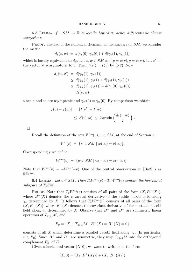
RANK RIGIDITY 69

6.3 Lemma. f : SM → R is locally Lipschitz, hence differentiable almosteverywhere.

Proof. Instead of the canonical Riemannian distance dS on SM , we considerthe metric

d1(v, w) = d(γv(0), γw(0)) + d(γv(1), γw(1))

which is locally equivalent to dS . Let v, w ∈ SM and p = π(v), q = π(w). Let v′ bethe vector at q asymptotic to v. Then f(v′) = f(v) by (6.2). Now

d1(w, v′) = d(γw(1), γv′(1))

≤ d(γw(1), γv(1) + d(γv(1), γv′(1))

≤ d(γw(1), γv(1)) + d(γv(0), γv′(0))

= d1(v, w)

since v and v′ are asymptotic and γv′(0) = γw(0). By comparison we obtain

|f(v)− f(w)| = |f(v′) − f(w)|

≤ ∠(v′, w) ≤ 2 arcsin

(d1(v, w)

2

).

�

Recall the definition of the sets W so(v), v ∈ SM , at the end of Section 3,

W so(v) = {w ∈ SM | w(∞) = v(∞)} .

Correspondingly we define

Wuo(v) = {w ∈ SM | w(−∞) = v(−∞)} .

Note that Wuo(v) = −W so(−v). One of the central observations in [Ba2] is asfollows.

6.4 Lemma. Let v ∈ SM . Then TvWso(v)+TvW

uo(v) contain the horizontalsubspace of TvSM .

Proof. Note that TvWso(v) consists of all pairs of the form (X,B+(X)),

where B+(X) denotes the covariant derivative of the stable Jacobi field alongγv determined by X . It follows that TvW

uo(v) consists of all pairs of the form(X,B−(X)), where B−(X) denotes the covariant derivative of the unstable Jacobifield along γv determined by X . Observe that B+ and B− are symmetric linearoperators of Tπ(v)M , and

E0 = {X ∈ Tπ(v)M | B+(X) = B−(X) = 0}

consists of all X which determine a parallel Jacobi field along γv. (In particular,v ∈ E0). Since B+ and B− are symmetric, they map Tπ(v)M into the orthogonal

complement E⊥0 of E0.

Given a horizontal vector (X, 0), we want to write it in the form

(X, 0) = (X1, B+(X1)) + (X2, B

−(X2))

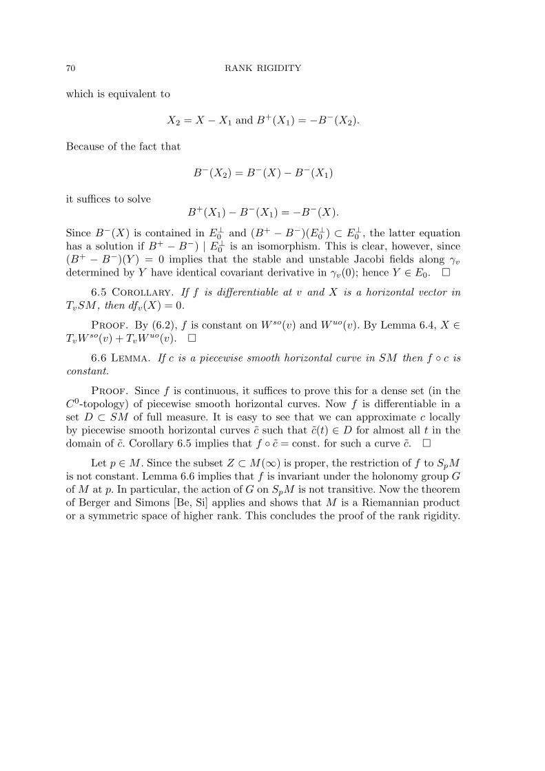
70 RANK RIGIDITY

which is equivalent to

X2 = X −X1 and B+(X1) = −B−(X2).

Because of the fact that

B−(X2) = B−(X) −B−(X1)

it suffices to solveB+(X1) −B−(X1) = −B−(X).

Since B−(X) is contained in E⊥0 and (B+ − B−)(E⊥

0 ) ⊂ E⊥0 , the latter equation

has a solution if B+ − B−) | E⊥0 is an isomorphism. This is clear, however, since

(B+ − B−)(Y ) = 0 implies that the stable and unstable Jacobi fields along γvdetermined by Y have identical covariant derivative in γv(0); hence Y ∈ E0. �

6.5 Corollary. If f is differentiable at v and X is a horizontal vector inTvSM , then dfv(X) = 0.

Proof. By (6.2), f is constant on W so(v) and Wuo(v). By Lemma 6.4, X ∈TvW

so(v) + TvWuo(v). �

6.6 Lemma. If c is a piecewise smooth horizontal curve in SM then f ◦ c isconstant.

Proof. Since f is continuous, it suffices to prove this for a dense set (in theC0-topology) of piecewise smooth horizontal curves. Now f is differentiable in aset D ⊂ SM of full measure. It is easy to see that we can approximate c locallyby piecewise smooth horizontal curves c such that c(t) ∈ D for almost all t in thedomain of c. Corollary 6.5 implies that f ◦ c = const. for such a curve c. �

Let p ∈M . Since the subset Z ⊂M(∞) is proper, the restriction of f to SpMis not constant. Lemma 6.6 implies that f is invariant under the holonomy group Gof M at p. In particular, the action of G on SpM is not transitive. Now the theoremof Berger and Simons [Be, Si] applies and shows that M is a Riemannian productor a symmetric space of higher rank. This concludes the proof of the rank rigidity.

INTRODUCTORY REMARKS 71

APPENDIX. ERGODICITY OF THE GEODESIC FLOW

M. Brin

We present here a reasonably self-contained and short proof of the ergodicityof the geodesic flow on a compact n-dimensional manifold of strictly negative sec-tional curvature. The only complete proof of specifically this fact was published byD.Anosov in [Ano1]. The ergodicity of the geodesic flow is buried there among quitea number of general properties of hyperbolic systems, heavily depends on most ofthe rest of the results and is rather difficult to understand, especially for somebodywhose background in smooth ergodic theory is not very strong. Other works on thisissue either give only an outline of the argument or deal with a considerably moregeneral situation and are much more difficult.

1. Introductory remarks

E.Hopf (see [Ho1], [Ho2]) proved the ergodicity of the geodesic flow for com-pact surfaces of variable curvature and for compact manifolds of constant sectionalcurvature in any dimension. The general case was established by D.Anosov andYa.Sinai (see [Ano1], [AnSi]) much later. Hopf’s argument is relatively short andvery geometrical. It is based on the property of the geodesic flow which Morse called“instability” and which is now commonly known as “hyperbolicity”. Although thelater proofs by Anosov and Sinai follow the main lines of Hopf’s argument, theyare considerably longer and more technical. The reason for the over 30 year gap be-tween the special and general cases is, in short, that length is volume in dimension 1but not in higher dimensions. More specifically, these ergodicity proofs extensivelyuse the horosphere H(v) as a function of the tangent vector v and the absolutecontinuity of a certain map p between two horospheres (the absolute continuityof the horospheric foliations). Since the horosphere H(v) depends on the infinitefuture of the geodesic γv determined by v, the function H(·) is continuous but, inthe general case, not differentiable even if the Riemannian metric is analytic. Asa result, the map p is, in general, only continuous. For n = 2 the horospheres are1-dimensional and the property of bounded volume distortion for p is equivalent toits Lipschitz continuity which holds true in special cases but is false in general.

The general scheme of the ergodicity argument below is the same as Hopf’s.Most ideas in the proof of the absolute continuity of the stable and unstable fo-liations are the same as in [Ano1] and [AnSi]. However, the quarter century de-velopment of hyperbolic dynamical systems and a couple of original elements have

Typeset by AMS-TEX

72 ERGODICITY OF THE GEODESIC FLOW

made the argument less painful and much easier to understand. The proof goesthrough with essentially no changes for the case of a manifold of negative sectionalcurvature with finite volume, bounded and bounded away from 0 curvature andbounded first derivatives of the curvature. For surfaces this is exactly Hopf’s result.The assumption of bounded first derivatives cannot be avoided in this argument.

The proof also works with no changes for any manifold whose geodesic flow isAnosov.

In addition to being ergodic, the geodesic flow on a compact manifold ofnegative sectional curvature is mixing of all orders, is a K-flow, is a Bernoulli flowand has a countable Lebesgue spectrum, but we do not address these strongerproperties here.

In Section 2 we list several basic facts from measure and ergodic theory. Con-tinuous foliations with C1-leaves and their absolute continuity are discussed in Sec-tion 3. In Section 4 we recall the definition of an Anosov flow and some of its basicproperties and prove the Holder continuity of the stable and unstable distributions.The absolute continuity of the stable and unstable foliations for the geodesic flowand its ergodicity are proved in Section 5.

2. Measure and ergodic theory preliminaries

A measure space is a triple (X,A, µ), where X is a set, A is a σ-algebraof measurable sets and µ is a σ-additive measure. We will always assume thatthe measure is finite or σ-finite. Let (X,A, µ) and (Y,B, ν) be measure spaces.A map ψ : X → Y is called measurable if the preimage of any measurable setis measurable; it is called nonsingular if, in addition, the preimage of a set ofmeasure 0 has measure 0. A nonsingular map from a measure space into itself iscalled a nonsingular transformation (or simply a transformation). Denote by λ theLebesgue measure on R. A measurable flow φ in a measure space (X,A, µ) is a mapφ : X × R → X such that (i) φ is measurable with respect to the product measureµ × λ on X × R and measure µ on X and (ii) the maps φt(·) = φ(·, t) : X → Xform a one-parameter group of transformations of X , that is φt ◦φs = φt+s for anyt, s ∈ R. The general discussion below is applicable to the discrete case t ∈ Z andto a measurable action of any locally compact group.

A measurable function f : X → R is φ-invariant if µ({x ∈ X : f(φtx) 6=f(x)}) = 0 for every t ∈ R. A measurable set B ∈ A is φ-invariant if its charac-teristic function 1B is φ-invariant. A measurable function f : X → R is strictlyφ-invariant if f(φtx) = f(x) for all x ∈ X, t ∈ R. A measurable set B is strictlyφ-invariant if 1B is strictly φ-invariant.

We say that something holds true mod 0 in X or for µ-a.e. x if it holds on asubset of full µ-measure in X . A null set is a set of measure 0.

2.1 Proposition. Let φ be a measurable flow in a measure space (X,A, µ)and let f : X → R be a φ-invariant function.

Then there is a strictly φ-invariant measurable function f such that f(x) =

f(x) mod 0.

Proof. Consider the measurable map Φ : X × R → X, Φ(x, t) = φtx,and the product measure ν in X × R. Since f is φ-invariant, ν({(x, t) : f(φtx) =f(x)}) = 1. By the Fubini theorem, the set

Af = {x ∈ X : f(φtx) = f(x) for a.e. t ∈ R}

MEASURE AND ERGODIC THEORY PRELIMINARIES 73

has full µ-measure. Set

f(x) =

{f(y) if φtx = y ∈ Af for some t ∈ R

0 otherwise .

If φtx = y ∈ Af and φsx = z ∈ Af then clearly f(y) = f(z). Therefore f is welldefined and strictly φ-invariant. �

2.2 Definition (Ergodicity). A measurable flow φ in a measure space(X,A, µ) is called ergodic if any φ-invariant measurable function is constant mod0, or equivalently, if any measurable φ-invariant set has either full or 0 measure.

The equivalence of the two definitions follows directly from the density of thelinear combinations of step functions in bounded measurable functions.

A measurable flow φ is measure preserving (or µ is φ-invariant) if µ(φt(B)) =µ(B) for every t ∈ R and every B ∈ A.

2.3 Ergodic Theorems. Let φ be a measure preserving flow in a finitemeasure space (X,A, µ). For a measurable function f : X → R set

f+T (x) =

1

T

∫ T

0

f(φtx) dt and f−T (x) =

1

T

∫ T

0

f(φ−tx) dt .

(1) (Birkhoff) If f ∈ L1(X,A, µ) then the limits f+(x) = limT→∞ f+T (x) and

f−(x) = limT→∞ f−T (x) exist and are equal for µ-a.e. x ∈ X, moreover

f+, f− are µ-integrable and φ-invariant.(2) (von Neumann) If f ∈ L2(X,A, µ) then f+

T and f−T converge in L2(X,A, µ)

to φ-invariant functions f+ and f−, respectively.

�

2.4 Remark. If f ∈ L2(X,A, µ), that is, if f2 is integrable, then f+ andf− represent the same element f of L2(X,A, µ) and f is the projection of f ontothe subspace of φ-invariant L2-functions. To see this let h be any φ-invariant L2-function. Since φ preserves µ we have∫

X

(f(x) − f(x))h dµ(x) =

∫

X

f(x)h(x) dµ(x)−∫

X

limT→∞

1

T

∫ T

0

f(φtx)h(x) dt dµ(x)

=

∫

X


X

limT→∞

1

T

∫ T

0

f(y)h(φ−1y) dt dµ(y)

=

∫

X


X

f(y)h(y) dµ(y) = 0 .

In the topological setting invariant functions are mod 0 constant on sets oforbits converging forward or backward in time.

Let (X,A, µ) be a finite measure space such that X is a compact metric spacewith distance d, µ is a measure positive on open sets and A is the µ-completion ofthe Borel σ-algebra. Let φ be a continuous flow in X , that is the map (x, t) → φtxis continuous. For x ∈ X define the stable V s(x) and unstable V u(x) sets by theformulas

(2.5)V s(x) = {y ∈ X : d(φtx, φty) → 0 as t→ ∞} ,V u(x) = {y ∈ X : d(φtx, φty) → 0 as t→ −∞} .


2.6 Proposition. Let φ be a continuous flow in a compact metric space Xpreserving a finite measure µ positive on open sets and let f : X → R be a φ-invariant measurable function.

Then f is mod 0 constant on stable sets and unstable sets, that is, there arenull sets Ns and Nu such that f(y) = f(x) for any x, y ∈ X \ Ns, y ∈ V s(x) andf(z) = f(x) for any x, z ∈ X \Nu, z ∈ V u(x).

Proof. We will only deal with the stable sets. Reversing the time gives thesame for the unstable sets. Assume WLOG that f is nonnegative.

For C ∈ R set fC(x) = min(f(x), C). Clearly fC is φ-invariant and it issufficient to prove the statement for fC with arbitrary C. For a natural m lethm : X → R be a continuous function such that

∫X|fC − hm| dµ(x) < 1

m . By theBirkhoff Ergodic Theorem,

h+m(x) = lim

T→∞

1

T

∫ T

0

fm(φtx) dt

exists a.e. Since µ and fC are φ-invariant, we have that for any t ∈ R

1

m>

∫

X

|fC(x) − hm(x)| dµ(x) =

∫

X

|fC(φty) − hm(φty)| dµ(y)

=

∫

X

|fC(y) − hm(φty)| dµ(y) .

Therefore

∫

X

∣∣fC(y)− 1

T

∫ T

0

hm(φty)∣∣ dt dµ(y) ≤ 1

T

∫ T

0

∫

X

|fC(y)− hm(φty)| dµ(y) dt <1

m.

Note that since hm is uniformly continuous, h+m(y) = h+

m(x) whenever y ∈ V s(x)and h+

m(x) is defined. Hence there is a set Nm of µ-measure 0 such that h+m exists

and is constant on the stable sets in X \Nm. Therefore, f+C (x) := limm→∞ h+

m(x)

is constant on the stable sets in X \ (∪Nm). Clearly fC(x) = f+C (x) mod 0. �

For differentiable hyperbolic flows in general and for the geodesic flow on anegatively curved manifold in particular, the stable and unstable sets are differen-tiable submanifolds of the ambient manifold Mn. The foliations W s and Wu intostable and unstable manifolds are called the stable and unstable foliations, respec-tively. Together with the 1-dimensional foliation W o into the orbits of the flow theyform three transversal foliations W s, Wu and W o of total dimension n. Any mod 0invariant function f is, by definition, mod 0 constant on the leaves of W o and, byProposition 2.6, is mod 0 constant on the leaves of W s and Wu. To prove ergodicityone must show that f is mod 0 locally constant. This would follow immediately ifone could apply a version of the Fubini theorem to the three foliations. Unfortu-nately the foliations W s and Wu are in general not differentiable and not integrable(see the next section for definitions). The applicability of a Fubini-type argumentdepends on the absolute continuity of W s and Wu which is discussed in the nextsection.

We will need the following simple lemma in the proof of Theorem 5.1.

ABSOLUTELY CONTINUOUS FOLIATIONS 75

2.7 Lemma. Let (X,A, µ), (Y,B, ν) be two compact metric spaces with Borelσ-algebras and σ-additive Borel measures and let pn : X → Y, n = 1, 2, ..., p : X →Y be continuous maps such that

(1) each pn and p are homeomorphisms onto their images,(2) pn converges to p uniformly as n→ ∞,(3) there is a constant C such that ν(pn(A)) ≤ Cµ(A) for any A ∈ A.

Then ν(p(A)) ≤ Cµ(A) for any A ∈ A.

Proof. It is sufficient to prove the statement for an arbitrary open ball Bin X . For δ > 0 let Bδ denote the δ-interior of B. Then p(Bδ) ⊂ pn(B) for n largeenough, and hence, ν(p(Bδ)) ≤ ν(pn(B)) ≤ Cµ(B). Observe now that ν(p(Bδ)) րν(p(B)) as δ ց 0 . �

3. Absolutely continuous foliations

Let M be a smooth n-dimensional manifold and let Bk denote the closed unitball centered at 0 in R

k. A partition W of M into connected k-dimensional C1-submanifolds W (x) ∋ x is called a k-dimensional C0-foliation of M with C1-leaves(or simply a foliation) if for every x ∈M there is a neighborhood U = Ux ∋ x anda homeomorphism w = wx : Bk ×Bn−k → U such that w(0, 0) = x and

(i) w(Bk, z) is the connected component WU (w(0, z)) of W (w(0, z)) ∩ U con-taining w(0, z),

(ii) w(·, z) is a C1-diffeomorphism of Bk onto WU (w(0, z)) which dependscontinuously on z ∈ Bn−k in the C1-topology.

We say that W is a C1-foliation if the homeomorphisms wx are diffeomor-phisms.

3.1 Exercise. Let W be a k-dimensional foliation of M and let L be an(n−k)- dimensional local transversal toW at x ∈M , that is, TxM = TxW (x)⊕TxL.Prove that there is a neighborhood U ∋ x and a C1 coordinat chart w : Bk ×Bn−k → U such that the connected component of L∩U containing x is w(0, Bn−k)and there are C1-functions fy : Bk → Bn−k, y ∈ Bn−k with the following proper-ties:

(i) fy depends continuously on y in the C1-topology;(ii) w(graph (fy)) = WU (w(0, y)).

We assume that M is a Riemannian manifold with the induced distance d.Denote by m the Riemannian volume in M and by mN denote the induced Rie-mannian volume in a C1-submanifold N .

3.2 Definition (Absolute continuity). Let L be a (n − k)-dimensionalopen (local) transversal for a foliation W , that is, TxL⊕ TxW (x) = TxM for everyx ∈ L. Let U ⊂ M be an open set which is a union of local “leaves”, that isU = ∪x∈LWU (x), where WU (x) ≈ Bk is the connected component of W (x) ∩ Ucontaining x.

The foliation W is called absolutely continuous if for any L and U as abovethere is a measurable family of positive measurable functions δx : WU (x) → R

(called the conditional densities) such that for any measurable subset A ⊂ U

m(A) =

∫

L

∫

WU (x)

1A(x, y)δx(y) dmW (x)(y) dmL(x) .


Note that the conditional densities are automatically integrable. Instead ofabsolute continuity we will deal with “transversal absolute continuity” which is astronger property, see Proposition 3.4.

3.3 Definition (Transversal absolute continuity). Let W be a fo-liation of M , x1 ∈ M , x2 ∈ W (x1) and let Li ∋ xi be two transversals toW, i = 1, 2. There are neighborhoods Ui ∋ xi, Ui ⊂ Li, i = 1, 2, and a home-omorphism p : U1 → U2 (called the Poincare map) such that p(x1) = x2 andp(y) ∈ W (y), y ∈ U1. The foliation W is called transversally absolutely continuousif the Poincare map p is absolutely continuous for any transversals Li as above,that is, there is a positive measurable function q : U1 → R (called the Jacobian ofp) such that for any measurable subset A ⊂ U1

mL2(p(A)) =

∫

U1

1Aq(y)dmL1(y) .

If the Jacobian q is bounded on compact subsets of U1 then W is called transversallyabsolutely continuous with bounded Jacobians.

3.4 Exercise. Is the Poincare map in Definition 3.3 uniquely defined?.

3.5 Proposition. If W is transversally absolutely continuous, then it is ab-solutely continuous.

Proof. Let L and U be as in Definition 3.2, x ∈ L and let F be an (n− k)-dimensional C1-foliation such that F (x) ⊃ L, FU (x) = L and U = ∪y∈WU (x)FU (y),see Figure 2. Obviously F is absolutely continuous and transversally absolutely con-tinuous. Let δy(·) denote the conditional densities for F . Since F is a C1-foliation, δis continuous, and hence, measurable. For any measurable set A ⊂ U , by the Fubinitheorem,

(3.6) m(A) =

∫

WU (x)

∫

FU (y)

1A(y, z)δy(z) dmF (y)(z) dmW (x)(y) .

Let py denote the Poincare map along the leaves of W from FU (x) = L toFU (y) and let qy(·) denote the Jacobian of py. It is not difficult to see that q is ameasurable function (see the exercise below). We have

∫

FU (y)

1A(y, z)δy(z) dmF (y)(z) =

∫

L

1A(py(s))qy(s)δy(py(s)) dmL(s)

and by changing the order of integration in (3.6) we get

(3.7) m(A) =

∫

L

∫

WU (x)

1A(py(s))qy(s)δy(py(s)) dmW (x)(y) dmL(s) .

Similarly, let ps denote the Poincare map along the leaves of F from WU (x) toWU (s), s ∈ L, and let qs denote the Jacobian of ps. We transform the integral overWU (x) into an integral over WU (s) using the change of variables r = py(s), y =p−1s (r)

∫

WU (x)

1A(py(s))qy(s)δy(py(s)) dmW (x)(y) =

∫

WU (s)

1A(r)qy(s)δy(r)q−1s (r) dmW (s)(r) .

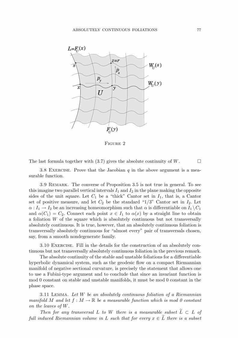
ABSOLUTELY CONTINUOUS FOLIATIONS 77

L=F

x

sz=r

yW

W

F

U

p

p

y

s

U(x)

U( )

U( y)

U(y)

s

Figure 2

The last formula together with (3.7) gives the absolute continuity of W . �

3.8 Exercise. Prove that the Jacobian q in the above argument is a mea-surable function.

3.9 Remark. The converse of Proposition 3.5 is not true in general. To seethis imagine two parallel vertical intervals I1 and I2 in the plane making the oppositesides of the unit square. Let C1 be a “thick” Cantor set in I1, that is, a Cantorset of positive measure, and let C2 be the standard “1/3” Cantor set in I2. Letα : I1 → I2 be an increasing homeomorphism such that α is differentiable on I1 \C1

and α(C1) = C2. Connect each point x ∈ I1 to α(x) by a straight line to obtaina foliation W of the square which is absolutely continuous but not transversallyabsolutely continuous. It is true, however, that an absolutely continuous foliation istransversally absolutely continuous for “almost every” pair of transversals chosen,say, from a smooth nondegenerate family.

3.10 Exercise. Fill in the details for the construction of an absolutely con-tinuous but not transversally absolutely continuous foliation in the previous remark.

The absolute continuity of the stable and unstable foliations for a differentiablehyperbolic dynamical system, such as the geodesic flow on a compact Riemannianmanifold of negative sectional curvature, is precisely the statement that allows oneto use a Fubini-type argument and to conclude that since an invariant function ismod 0 constant on stable and unstable manifolds, it must be mod 0 constant in thephase space.

3.11 Lemma. Let W be an absolutely continuous foliation of a Riemannianmanifold M and let f : M → R be a measurable function which is mod 0 constanton the leaves of W .

Then for any transversal L to W there is a measurable subset L ⊂ L of

full induced Riemannian volume in L such that for every x ∈ L there is a subset


W (x) ⊂W (x) of full induced Riemannian volume in W (x) on which f is constant.

Proof. Given a transversal L break it into smaller pieces Li and considerneighborhoods Ui as in the definition of absolute continuity. Let N be the null setsuch that f is constant on the leaves of W in M \N and let Ni = N ∩ Ui. By the

absolute continuity of W for each i there is a subset Li of full measure in Li such

that for each x ∈ Li the complement WUi(x) of Ni in WUi

(x) has full measure inthe local leaf. �

Two foliations W1 and W2 of a Riemannian manifold M are transversal ifTxW1(x) ∩ TxW2(x) = {0} for every x ∈M .

3.12 Proposition. Let M be a connected Riemannian manifold and let W1,W2 be two transversal absolutely continuous foliations on M of complementarydimensions, that is TxM = TxW1(x)⊕TxW2(x) for every x ∈M (the sum is directbut not necessarily orthogonal). Assume that f : M → R is a measurable functionwhich is mod 0 constant on the leaves of W1 and mod 0 constant on the leaves ofW2.

Then f is mod 0 constant in M .

Proof. Let Ni ⊂M, i = 1, 2, be the null sets such that f is constant on theleaves of Wi in Mi = M \ Ni. Let x ∈ M and let U ∋ x be a small neighborhood.By Lemma 3.11, since W1 is absolutely continuous, there is y arbitrarily close to

x whose local leaf WU1(y) intersects M1 by a set M1(y) of full measure. Since W2

is absolutely continuous, for almost every z ∈ M1(y) the intersection W2 ∩M2 hasfull measure. Therefore f is mod 0 constant in a neighborhood of x. Since M isconnected, f is mod 0 constant in M . �

The previous proposition can be applied directly to the stable and unstablefoliations of a volume preserving Anosov diffeomorphism to prove its ergodicity(after establishing the absolute continuity of the foliations). The case of flows ismore difficult since there are three foliations involved – stable, unstable and thefoliation into the orbits of the flow. In that case one gets a pair of transversalabsolutely continuous foliations of complementary dimensions by considering thestable foliation W s and the weak unstable foliation Wuo whose leaves are the orbitsof the unstable leaves under the flow.

Two transversal foliations Wi of dimensions di, i = 1, 2, are integrable andtheir integral hull is a (d1 + d2)-dimensional foliation W if

W (x) = ∪y∈W1(x)W2(y) = ∪z∈W2(x)W1(z) .

3.13 Lemma. Let Wi, i = 1, 2, be transversal integrable foliations of a Rie-mannian manifold Mwith integral hull W such that W1 is a C1-foliation and W2

is absolutely continuous.Then W is absolutely continuous.

Proof. Let L be a transversal for W . For a properly chosen neighborhood

U in M the set L = ∪x∈LW1U (x) is a transversal for W2. Since W2 is absolutelycontinuous, we have for any measurable subset A ⊂ U

m(A) =

∫

eL

∫

W2U (y)

1A(y, z)δy(z) dmW2U (y)(z) dmeL(y) .

HOLDER CONTINUITY OF INVARIANT DISTRIBUTIONS 79

Since L is foliated by W1-leaves,

∫

eL

dmeL(x) =

∫

L

∫

W1U (x)

j(x, y) dm1U(x)(y) dml(x)

for some positive measurable function j. The absolute continuity of W followsimmediately. �

We will need several auxiliary statements to prove the absolute continuity ofthe stable and unstable foliations of the geodesic flow.

4. Anosov flows and the Holder continuity of invariant distributions

For a differentiable flow denote by W o the foliation into the orbits of the flowand by Eo the line field tangent to W o.

4.1 Definition (Anosov flow). A differentiable flow φt in a compact Rie-mannian manifold M is called Anosov if it has no fixed points and there are distri-butions Es, Eu ⊂ TM and constants C, λ > 0, λ < 1, such that for every x ∈ Mand every t ≥ 0

(a) Es(x) ⊕Eu(x) ⊕ Eo(x) = TxM ,

(b) ‖dφtxvs‖ ≤ Cλt‖vs‖ for any vs ∈ Es(x) ,

(c) ‖dφ−tx vu‖ ≤ Cλt‖vu‖ for any vu ∈ Eu(x)

It follows automatically from the definition that the distributions Es and Eu

(called the stable and unstable distributions, respectively) are continuous, invariantunder the derivative dφt and their dimensions are (locally) constant and positive.To see this observe that if a sequence of tangent vectors vk ∈ TM satisfies (b) andvk → v ∈ TM as k → ∞, then v satisfies (b), and similarly for (c).

The stable and unstable distributions of an Anosov flow are integrable in thesense that there are stable and unstable foliations W s and Wu whose tangent dis-tributions are precisely Es and Eu. The manifolds W s(x) and Wu(x) are the stableand unstable sets as described in (2.5). This is proved in any book on differentiablehyperbolic dynamics. The geodesic flow on a manifold M of negative sectional cur-vature is Anosov. Its stable and unstable subspaces are the spaces of stable andunstable Jacobi fields perpendicular to the geodesic and the (strong) stable andunstable manifolds are unit normal bundles to the horospheres (see Chapter IV). Ifthe sectional curvature of M is pinched between −a2 and −b2 with 0 < a < b thenInequalities (b) and (c) of Definition 4.1 hold true with λ = e−a (see PropositionIV.2.9).

For subspaces H1, H2 ⊂ TxM define the distance dist (H1, H2) as the Haus-dorff distance between the unit spheres in H1 and H2. We say that H2 is θ-transversal to H1 if min ‖v1 − v2‖ ≥ θ, where the minimum is taken over all unitvectors v1 ∈ H1, v2 ∈ H2.

Set Eso(x) = Es(x) ⊕ Eo(x), Euo(x) = Eu(x) ⊕ Eo(x). By compactness,the pairs Es(x), Euo(x) and Eu(x), Eso(x) are θ-transversal with some θ > 0independent of x.


4.2 Lemma. Let φt be an Anosov flow. Then for every θ > 0 there is C1 > 0such that for any subspace H ⊂ TxM with the same dimension as Es(x) and θ-transverssal to Eu0(x) and any t ≥ 0

dist (dφ−t(x)H,Es(φ−tx)) ≤ C1λtdist (H,Es(x)) .

Proof. Let v ∈ H, ‖v‖ = 1, v = vs + vuo, vs ∈ Es(x), vuo ∈ Euo(x).Then ‖vs‖ > const · θ, dφ−t(x)vs ∈ Es(φ−tx), dφ−t(x)vuo ∈ Euo(φ−tx) and‖dφ−t(x)vuo‖ ≤ const · ‖vuo‖, ‖dφ−t(x)vs‖ ≥ C−1λ−t‖vs‖. �

A distribution E ⊂ TM is called Holder continuous if there are constantsA, α > 0 such that for any x, y ∈M

dist(E(x), E(y)) ≤ Ad(x, y)α ,

where dist(E(x), E(y)) denotes, for example, the Hausdorff distance in TM betweenthe unit spheres in E(x) and E(y). The numbers A and α are called the Holderconstant and exponent, respectively.4.3 Adjusted metric. Many arguments in hyperbolic dynamical systems becometechnically easier if one uses the so-called adjusted metric in M which is equivalentto the original Riemannian metric. Let φt : M → M be an Anosov flow. Letβ ∈ (λ, 1). For vo ∈ Eo, vs ∈ Es, vu ∈ Eu and T > 0 set

|vo| = ‖vo‖ ; |vs| =

∫ T

0

‖dφτvs‖βτ

dτ, |vu| =

∫ T

0

‖dφ−τvs‖βτ

dτ,

|vo + vs + vu|2 = |vo|2 + |vs|2 + |vu|2 .

Note that since β > λ, the integrals∫∞

0‖dφτvs‖βτ dτ and

∫∞

0‖dφ−τvs‖

βτ dτ converge.

For t > 0 we have

|dφtvs| =

∫ T

0

‖dφt+τvs‖βτ

dτ = βt∫ T+t

t

‖dφτvs‖βτ

dτ

= βt

(|vs| −

∫ t

0

‖dφτvs‖βτ

dτ +

∫ T+t

T

‖dφτvs‖βτ

dτ

).

For T large enough the second integral in parentheses is less than the first one andwe get

|dφtvs| ≤ βt|vs|and similarly for vu. Note that Es, Eu and Eo are orthogonal in the adjustedmetric.

The metric | · | is clearly smooth and equivalent to ‖·‖ and in the hyperbolicityinequalities of Definition 4.1 λ is replaced by β and C by 1.

In the next proposition we prove the Holder continuity of Es and Eu. This wasfirst proved by Anosov (see [Ano2]). To make the exposition complete we present asimilar but shorter argument here. It uses the main idea of a more general argumentfrom [BrK1] (see Theorem 5.2). To eliminate a couple of constants we assume thatthe flow is C2 but the argument works equally well for a C1-flow whose derivativeis Holder continuous.

HOLDER CONTINUITY OF INVARIANT DISTRIBUTIONS 81

4.4 Proposition. Distributions Es, Eu, Eso, Euo of a C2 Anosov flow φt

are Holder continuous.

Proof. Since Eo is smooth and since the direct sum of two transversal Holdercontinuous distribution is clearly Holder continuous, it is sufficient to prove thatEs and Eu are Holder continuous. We consider only Es, the Holder continuity ofEu can be obtained by reversing the time. As we mentioned above, the hyperbol-icity conditions (see Definition 4.1) are closed, and hence, all four distributions arecontinuous. Obviously a distribution which is Holder continuous in some metric isHolder continuous in any equivalent metric. Fix β ∈ (λ, 1) and use the adjustedmetric for β with an appropriate T . We will not attempt to get the best possibleestimates for the Holder exponent and constant here.

The main idea is to consider two very close points x, y ∈M and their imagesφmx and φmy. If the images are reasonably close, the subspaces Es(φmx) andEsφmy) are (finitely) close by continuity. Now start moving the subspaces “back”to x and y by the derivatives dφ−1. By the invariance of Es under the derivative,dφ−kEs(φmx) = Es(φm−kx). By Lemma 4.2, the image of Es(φmy) under dφmxφ

−k

is exponentially in k close to Es(φm−kx). An exponential estimate on the distancebetween the corresponding images of x and y allows us to replace dφ−1 along theorbit of y by dφ−1 along the orbit of x.

To abbreviate the notation we use φ instead of φ1. Fix γ ∈ (0, 1), let x, y ∈Mand choose q such that γq+1 < d(x, y) ≤ γq. Let D ≥ max ‖dφ‖ and fix ε > 0. Letm be the integer part of (log ε− q log γ)/ logD. Then

d(φix, φiy) ≤ d(x, y)Di ≤ γqDi and d(φix, φiy) ≤ ε, i = 0, 1, ..., m .

Assume that γ is small enough so thatm is large. Consider a system of small enoughcoordinate neighborhoods Ui ⊃ Vi ∋ φix identified with small balls in TφixM bydiffeomorphisms with uniformly bounded derivatives and such that φ−1Vi ⊂ Ui−1.Assume that ε is small enough, so that φiy ∈ Vi for i ≤ m. We identify the tangentspaces TzM for z ∈ Vi with TφixM and the derivatives (dzφ)−1 with matriceswhich may act on tangent vectors with footpoints anywhere in Vi. In the argumentbelow we estimate the distance between Es(x) and the parallel translate of Es(y)from y to x. Since the distance function between points is Lipschitz continuous, ourestimate implies the Holder continuity of Es.

Let vy ∈ Es(φmy), |vy| > 0, vk = dφ−kvy = vsk + vuok , vs ∈ Es(φm−kx), vuo ∈Euo(φm−kx), k = 0, 1, ..., m,. Fix κ ∈ (

√β, 1). We use induction on k to show that if

ε is small enough then ‖vuok ‖/‖vsk‖ ≤ δκk for k = 0, ...m and a small δ > 0. For k = 0the above inequality is satisfied for a small enough ε since Es is continuous. Assumethat the inequality holds true for some k. Set (dφm−kxφ)−1 = Ak, (dφm−kyφ)−1 =

Bk. By the choice of D we have ‖Ak − Bk‖ ≤ const · γqDm−k =: ηk ≤ const · ε,where the constant depends on the maximum of the second derivatives of φ. Wehave

|Akvsk| ≥ β−1|vsk|, |Akvuok | ≤ |vuok |,vk+1 = Bkvk = Akvk + (Bk − Ak)vk = Ak(v

sk + vuok ) + (Bk − Ak)vk .

Therefore|vuok+1||vsk+1|

≤ |Akvuok | + ‖Ak −Bk‖ · |vk||Akvsk| − |(Ak −Bk)vk|

≤ (δκk + ηk)|vk|

β−1(|vk| − |vuok |) − ηk|vk|

≤((δκk + ηk)

√β)( |vk|

|vk|(1 − βηk − δκk)

√β

).


By the choice of m and D above, ηk = const · γqDm−k ≤ const · εD−k, and hencethe inequality for k + 1 holds true provided D is big enough, ε is small enough,√β < κ and δ is chosen so that the last factor is less than 1.

For k = m we get that |vuom |/|vsm| ≤ δκm and, by the choice of m,

|vuom ||vsm| ≤ const · γ−(q+1) log κ

log D ≤ const · dist (x, y)−log κlog D .

Note that by varying vy we obtain all vectors vm ∈ Es(y). �

5. Proof of absolute continuity and ergodicity

We assume now thatM is a compact boundaryless m-dimensional Riemannianmanifold of strictly negative sectional curvature. For v ∈ SM set Es(v) = {(X, Y ) :

Y = J′

X(0)}, where JX is the stable field along γv which is perpendicular to γv andsuch that JX(0) = X . Set Eu(v) = −Es(−v). By Section IV.2, the distributionsEs and Eu are the stable and unstable distributions of the geodesic flow gt in thesense of Definition 4.1. By Section IV.3, the distributions Es and Eu are integrableand the leaves of the corresponding foliations W s and Wu of SM are the twocomponents of the unit normal bundles to the horospheres.

5.1 Theorem. Let M be a compact Riemannian manifold with a C3-metric ofnegative sectional curvature. Then the foliationsW s and Wu of SM into the normalbundles to the horospheres are transversally absolutely continuous with boundedJacobians.

Proof. We will only deal with the stable foliation W s. Reverse the time forthe geodesic flow gt to get the statement for Wu. Let Li be two C1-transversalsto W s and let Ui and p be as in Definition 3.3. Denote by Σn the foliation of SMinto “inward” spheres, that is, each leaf of Σn is the set of unit vectors normal toa sphere of radius n in M and pointing inside the sphere. Let Vi ⊂ Ui be closedsubsets such that V2 contains a neighborhood of p(V1). Denote by pn the Poincaremap for Σn and transversals Li restricted to V1. We will use Lemma 16 to provethat the Jacobian q of p is bounded. By the construction of the horospheres, pn ⇉ pas n→ ∞. We must show that the Jacobians qn of pn are uniformly bounded.

To show that the Jacobians qn of the Poincare maps pn : L1 → L2 are uni-formly bounded we represent pn as the following composition

(5.2) pn = g−n ◦ P0 ◦ gn ,

where gn is the geodesic flow restricted to the transversal L1 and P0 : gn(L1) →gn(L2) is the Poincare map along the vertical fibers of the natural projection π :SM → M . For a large enough n, the spheres Σn are close enough to the stablehorospheres W s, and hence, are uniformly transverse to L1 and L2 so that pn iswell defined on V1. Let vi ∈ Vi, i = 1, 2, and pn(v1) = v2. Then π(gnv1) = π(gnv2)and p0(g

nv1) = gnv2. Let J ik denote the Jacobian of the time 1 map g1 in thedirection of T ik = Tgkvi

Li at gkvi ∈ Li, i = 1, 2, that is J ik = | det(dg1(gkvi)∣∣T i

k

)‖ .If J0 denotes the Jacobian of P0, we get from (5.2)

PROOF OF ABSOLUTE CONTINUITY AND ERGODICITY 83

(5.3) qn(v1) =n−1∏

k=0

(J2k )

−1 · J0 ·n−1∏

k=0

(J1k ) = J0(g

nv1) ·n−1∏

k=0

(J1k/J

2k ) .

By Lemma 4.2, for a large n the tangent plane at gnv1 to the image gn(L1)is close to Eso(gnv1), and hence, is uniformly (in v1) transverse to the unit sphereSxM at the point x = π(gnv1) = π(gnv2). Note also that the unit spheres form afixed smooth foliation of SM . Therefore the Jacobian J0 is bounded from aboveuniformly in v1.

We will now estimate from above the last product in (5.3). By PropositionIV.2.10,

d(gkv1, gkv2) ≤ const · exp(−ak) · d(v1, v2) .

Hence, by the Holder continuity of Euo,

dist(Euo(gkv1), Euo) ≤ const · d(gkv1, gkv2)α ≤ const · exp(−akα) .

Together with Lemma 4.2 this implies that

dist(T 1k , T

2k ) ≤ const · exp(−βk)

with some β > 0. Our assumptions on the metric imply that the derivative dg1(v)is Lipschitz continuous in v. Therefore its determinants in two exponentially closedirections are exponentially close, that is ‖J1

k−J2k‖ ≤ const·exp(−γk). Observe now

that ‖J ik‖ is uniformly separated away from 0 by the compactness of M . Thereforethe last product in (5.3) is uniformly bounded in n and v1. By Lemma 2.7, theJacobian q of the Poincare map p is bounded. �

We will need the following property of absolutely continuous foliations in theproof of Theorem 5.5.

5.4 Lemma. Let W be an absolutely continuous foliation of a manifold Q andlet N ⊂ Q be a null set. Then there is a null set N1 such that for any x ∈ Q \N1

the intersection W (x) ∩N has conditional measure 0 in W (x).

Proof. Consider any local transversal L for W . Since W is absolutely con-

tinuous, there is a subset L of full mL measure in L such that mW (x)(N) = 0 for

x ∈ L. Clearly the set ∪x∈eLW (x) has full measure. �

5.5 Theorem. Let M be a compact Riemannian manifold with a C3 metricof negative sectional curvature. Then the geodesic flow gt : SM → SM is ergodic.

Proof. Let m be the Riemannian volume in M , λx be the Lebesgue measurein SxM, x ∈M and µ be the Liouville measure in SM , dµ(x, v) = dm(x)×dλx(v).Since M is compact, m(M) < ∞ and µ(SM) = m(M) · λx(SxM). The localdifferential equation determining the geodesic flow gt is

x = v, v = 0 .

By the divergence theorem, the Liouville measure is invariant under gt (see alsoSection IV.1). Hence the Birkhoff Ergodic Theorem and Proposition 2.6 hold truefor gt.


Since the unstable foliation Wu is absolutely continuous and the foliation W o

into the orbits of gt is C1, the integral hull Wuo is absolutely continuous by Lemma3.13. Let f : SM → R be a measurable g-invariant function. By Proposition 2.1, fcan be corrected on a set of Liouville measure 0 to a strictly g-invariant functionf . By Proposition 2.6, there is a null set Nu such that f is constant on the leavesof Wu in SM \ Nu. Applying Lemma 5.4 twice we obtain a null set N1 such thatNu is a null set in Wuo(v) and in Wu(v) for any v ∈ SM \ N1. It follows that fis mod 0 constant on the leaf Wu(v) and, since it is strictly g-invariant, is mod 0constant on the leaf Wuo(v). Hence f is mod 0 constant on the leaves of Wuo. Nowapply Proposition 3.12 to W s and Wuo. �

BIBLIOGRAPHY 85

BIBLIOGRAPHY

[AbS1] U. Abresch & V. Schroeder, Graph manifolds, ends of negatively curved spaces and the

hyperbolic 120-cell space, J. Differential Geometry 35 (1992), 299–336.

[AbS2] U. Abresch & V. Schroeder, Analytic manifolds of nonpositive curvature, Preprint.

[ACBu] N. A’Campo & M. Burger, Reseaux arithmetiques et commensurateur d’apres G.A.Margulis, Inventiones math. 116 (1994), 1–25.

[Ad] S. Adams, Rank rigidity for foliations by manifolds of nonpositive curvature.

[Alb1] S.I. Al’ber, On n-dimensional problems in the calculus of variations in the large, Soviet

Math. Doklady 5 (1964), 700–804.

[Alb2] S.I. Al’ber, Spaces of mappings into a manifold with negative curvature, Soviet Math.

Doklady 9 (1967), 6–9.

[Alek] D. V. Alekseevskiı, Homogeneous Riemannian spaces of negative curvature, Math. USSR

Sbornik 25 (1975), 87–109.

[AB1] S.B. Alexander & R.L. Bishop, The Hadamard-Cartan theorem in locally convex metricspaces, L’Enseignement Math. 36 (1990), 309–320.

[AB2] S.B. Alexander & R.L. Bishop, Comparison theorems for curves of bounded geodesiccurvature in metric spaces of curvature bounded above, Differential Geometry and Its

Applications (to appear).

[ABB] S.B. Alexander, I.D. Berg & R.L. Bishop, Geometric curvature bounds in Riemannian

manifolds with boundary, Trans. Amer. Math. Soc. 339 (1993), 703–716.

[Al1] A.D. Alexandrov, A theorem on triangles in a metric space and some applications,

Trudy Math. Inst. Steklov 38 (1951), 5–23. (Russian; translated into German and com-

bined with more material in [Ale2])

[Al2] A.D. Alexandrov, Uber eine Verallgemeinerung der Riemannschen Geometrie, Schr.

Forschungsinst. Math. Berlin 1 (1957), 33–84.

[Al3] A.D. Alexandrov, Ruled surfaces in metric spaces, Vestnik Leningrad Univ. 12 (1957),

5–26. (Russian)

[AlBe] A.D. Alexandrov & V.N. Berestovskiı, Generalized Riemannian spaces, Math. Ency-

clopaedia 4, 1984, pp. 1022–1026; English translation published by Kluver, Dordrecht

[AlBN] A.D. Alexandrov, V.N. Berestovskiı & I.G. Nikolaev, Generalized Riemannian spaces,

Russian Math. Surveys 41 (1986), 1–54.

[AlRe] A.D. Alexandrov & Yu.G. Reshetnyak, General Theory of Irregular Curves, Kluwer

Academic Publishers, Dordrecht, Boston, London, 1989.

[AlZa] A.D. Alexandrov & V.A. Zalgaller, Intrinsic geometry of surfaces, Translations of Math.Monographs 15, Amer. Math. Soc., Providence, Rhode Island, 1967.

[AloB] J.M. Alonso & M.R. Bridson, Semihyperbolic groups, Proceedings LMS (3) 70 (1995),56–114.

[AnDG] F.D. Ancel, M.W. Davis & C.R.Guilbault, CAT (0) reflection manifolds, Preprint, OhioState University (1993).

[AnGu] F.D. Ancel & C.R. Guilbault, Interiors of compact contractible n-manifolds are hyper-bolic (n ≥ 5), Preprint (1993).

[Anc1] A. Ancona, Negatively curved manifolds, elliptic operators, and the Martin boundary,

Annals of Math. 125 (1987), 495–536.

Typeset by AMS-TEX


[Anc2] A. Ancona, Sur les fonctions propres positives des varietes de Cartan-Hadamard, Com-

ment. Math. Helvetici 64 (1989), 62–83.

[Anc3] A. Ancona, Theorie du potentiel sur les graphes et les varietes, Ecole d’Ete de Proba-

bilites de Saint-Flour XVIII (P.L. Hennequin, ed.), Lecture Notes Maths. 1427, Springer-

Verlag, 1990, pp. 5–112.

[Anc4] A. Ancona, Convexity at infinity and Brownian motion on manifolds with unboundednegative curvature, Revista Matematica Iberoamericana 10 (1994), 189–220.

[And] M. Anderson, The Dirichlet problem at infinity for manifolds of negative curvature, J.

Differential Geometry 18 (1983), 701–721.

[AnSo] M. Anderson & R. Schoen, Positive harmonic functions on complete manifolds of neg-

ative curvature, Annals of Math. 121 (1985), 429–461.

[AnSr] M. Anderson & V. Schroeder, Existence of flats in manifolds of nonpositive curvature,Invent. math. 85 (1986), 303–315.

[Ano1] D.V. Anosov, Geodesic flows on closed Riemannian manifolds with negative curvature,Proc. Steklov Institute 90 (1967).

[Ano2] D.V. Anosov, Tangent fields of transversal foliations in U-systems, Math. Notes Acad.

Sci. USSR 2:5 (1968), 818–823.

[AnSi] D.V. Anosov & Ya.G. Sinai, Some smooth ergodic systems, Russian Math. Surveys 22:5

(1967), 103–168.

[ArFa] C.S. Aravinda & F.T. Farrell, Rank 1 aspherical manifolds which do not support anynonpositively curved metric, Preprint 1993.

[Av] A. Avez, Varietes Riemanniennes sans points focaux, C. R. Acad. Sci. Paris 270 (1970),

188–191.

[AzW1] R. Azencott & E. Wilson, Homogeneous manifolds with negative curvature, I, Transac-

tions Amer. Math. Soc. 215 (1976), 323–362.

[AzW2] R. Azencott & E. Wilson, Homogeneous manifolds with negative curvature, II, MemoirsAmer. Math. Soc. 178 (1976).

[Bab1] M. Babillot, Theorie du renouvellement pour des chaines semi-markoviennes tran-sientes, Ann. Inst. Henri Poincare 24 (1988), 507–569.

[Bab2] M. Babillot, Comportement asymptotique du mouvement brownien sur une variete ho-

mogene a courbure sectionelle negative ou nulle, Ann. Inst. Henri Poincare 27 (1991),

61–90.

[Bab3] M. Babillot, Potential at infinity and Martin boundary for symmetric spaces, Harmonicanalysis and discrete potential theory (Picardello, ed.), Proceedings Frascati Conference,

Plenum Press, New York, 1992.

[Bab4] M. Babillot, A probabilistic approach to heat diffusion on symmetric spaces, J. Theo-

retical Probability 7 (1994), 599–607.

[Bab5] M. Babillot, Asymptotics of Green functions on a class of solvable Lie groups, Preprint,Paris VI (1994).

[Ba1] W. Ballmann, Axial isometries of manifolds of nonpositive curvature, Math. Annalen

259 (1982), 131–144.

[Ba2] W. Ballmann, Nonpositively curved manifolds of higher rank, Annals of Math. 122

(1985), 597–609.

[Ba3] W. Ballmann, On the Dirichlet problem at infinity for manifolds of nonpositive curva-ture, Forum Math. 1 (1989), 201–213.

[Ba4] W. Ballmann, The Martin boundary of certain Hadamard manifolds, Nieprint, Bonn1990.

[Ba5] W. Ballmann, Singular spaces of non-positive curvature, Sur les groupes hyperboliques

d’apres Mikhael Gromov (E. Ghys & P. de la Harpe, eds.), Progress in Math. 61,

Birkhauser, Boston-Basel-Berlin, 1990.

[BB1] W. Ballmann & M. Brin, On the ergodicity of geodesic flows, Ergodic Theory & Dy-namical Systems 2 (1982), 311–315.

[BB2] W. Ballmann & M. Brin, Polygonal complexes and combinatorial group theory, Geo-

metriae Dedicata 50 (1994), 165–191.

[BB3] W. Ballmann & M. Brin, Orbihedra of nonpositive curvature, SFB256-Preprint 367,

Universitat Bonn (1994).

[BBB1] W. Ballmann, M. Brin & K. Burns, On surfaces with no conjugate points, J. DifferentialGeometry 25 (1987), 249–273.

BIBLIOGRAPHY 87

[BBB2] W. Ballmann, M. Brin & K. Burns, On the differentiability of horocycles and horocyclic

foliations, J. Differential Geometry 26 (1987), 337–347.

[BBE] W. Ballmann, M. Brin & P. Eberlein, Structure of manifolds of nonpositive curvature,I, Annals of Math. 122 (1985), 171–203.

[BBS] W. Ballmann, M. Brin & R. Spatzier, Structure of manifolds of nonpositive curvature,

II, Annals of Math. 122 (1985), 205–235.

[BaBu] W. Ballmann & S. Buyalo, Nonpositively curved metrics on 2-polyhedra, Math. Zeit-schrift (to appear).

[BaEb] W. Ballmann & P. Eberlein, Fundamental groups of manifolds of nonpositive curvature,

J. Differential Geometry 25 (1987), 1–22.

[BGS] W. Ballmann, M. Gromov & V. Schroeder, Manifolds of nonpositive curvature (1985),

Birkhauser, Boston-Basel-Stuttgart.

[BaL1] W. Ballmann & F. Ledrappier, The Poisson boundary for rank one manifolds and theircocompact lattices, Forum Math. 6 (1994), 301–313.

[BaL2] W. Ballmann & F. Ledrappier, Discretization of positive harmonic functions on Rie-

mannian manifolds and Martin boundary (to appear).

[BaWo] W. Ballmann &M. Wojtkowski, An estimate for the measure theoretic entropy of geo-

desic flows, Ergodic Theory & Dynamical Systems 9 (1989), 271–279.

[BanS] V. Bangert & V. Schroeder, Existence of flat tori in analytic manifolds of nonpositive

curvature, Annales Sci. Ec. Norm. Sup. 24 (1991), 605–634.

[Bar] S. Barre, Polyedres finis de dimension 2 a courbure ≤ 0 et de rang 2, ENS, Lyon (1994).

[Ben1] N. Benakli, Polyedre a geometrie locale donnee, C. R. Acad. Sci. Paris 313 (1991),

561–564.

[Ben2] N. Benakli, Polyedre hyperbolique a groupe d’automorphismes non discret, C. R. Acad.Sci. Paris 313 (1991), 667–669.

[Ben3] N. Benakli, Polyedre avec un nombre fini de types de sommets, C. R. Acad. Sci. Paris.

[Ben4] N. Benakli, Polygonal complexes I: combinatorial and geometric properties, Preprint,

Princeton University (1993).

[BFL] Y. Benoist, P. Foulon & F. Labourie, Flots d’Anosov a distributions stable et instabledifferentiables, J. Amer. Math. Soc. 5 (1992), 33–74.

[Ber1] V. Berestovskiı, On the problem of finite dimensionality of Busemann’s G-space, Sib.

Mat. Z. 18 (1977), 219–221. (Russian)

[Ber2] V. Berestovskiı, Borsuk’s problem on the metrization of a polyhedron, Dokl. Akad. Nauk

CCCP 27 (1983), 273–277 (Russian); English translation in: Soviet Math. Doklady 27(1983), 56–59.

[Ber3] V. Berestovskiı, Spaces with bounded curvature and distance geometry, Sib. Mat. Z. 27

(1986), 11–25 (Russian); English translation in: Siberian Math. J. 27 (1986), 8–19.

[Ber4] V. Berestovskiı, Manifolds with intrinsic metric with one-sided bounded curvature inthe sense of A.D. Alexandrov, Math. Physics, Analysis, Geometry 1:1 (1994), 41–59.

(Russian, summary in Ukranian)

[Ber5] V. Berestovskiı, On Alexandrov’s spaces with curvature bounded from above, Russian

Acad. Sci. Doklady (former Soviet Math. Dokl.) (to appear).

[BerN] V.N. Berestovskiı & I.G. Nikolaev, Multidimensional generalized Riemannian spaces,Geometry IV (Yu.G. Reshetnyak, ed.), Encyclopaedia of Math. Sciences 70, Springer-

Verlag, Berlin-Heidelberg-New York..., 1993, pp. 165–243.

[Be] M. Berger, Sur les groupes d’holonomie homogene des varietes a connexion affine et

des varietes riemanniennes, Bull. Soc. Math. France 83 (1953), 279–330.

[BCG] G. Besson, G. Courtois & S. Gallot, Volumes, entropies et rigidites des espaces locale-ment symetriques de courbure strictement negative, C. R. Acad. Sci. Paris 319 (1994),

81–84.

[BiGe] R. Bieri & R. Geoghegan, Kernels of actions on nonpositively curved spaces, Preprint,Binghamton University (1995).

[BiON] R. Bishop & B. O’Neill, Manifolds of negative curvature, Transactions Amer. Math.

Soc. 145 (1969), 1–49.

[Bl] L.M. Blumenthal, Theory and applications of distance geometry, Oxford at the Claren-

don Press, 1953.

[BlMe] L.M. Blumenthal & K. Menger, Studies in geometry, W.H. Freeman and Company, SanFrancisco, 1970.


[Bor1] A. Borbely, A note on the Dirichlet problem at infinity for manifolds of negative cur-

vature, Proceedings Amer. Math. Soc. 114 (1992), 865–872.

[Bor2] A. Borbely, On convex hulls in negatively curved manifolds, Preprint.

[Bow] B.H. Bowditch, A class of incomplete non-positively curved manifolds, Preprint, Uni-

versity of Melbourne (1991).

[Bri1] M.R. Bridson, Geodesics and curvature in metric simplicial complexes, Group theoryfrom a geometrical viewpoint (E. Ghys, A. Haefliger & A. Verjovsky, eds.), Proceedings

ICTP, Trieste, World Scientific, Singapore, 1991.

[Bri2] M.R. Bridson, On the existence of flat planes in spaces of nonpositive curvature, Pro-

ceedings Amer. Math. Soc. (to appear).

[BrHa] M.R. Bridson & A. Haefliger, Spaces of nonpositive curvature, In preparation.

[BrK1] M. Brin & Y. Kifer, Harmonic measures on covers of compact surfaces of nonpositivecurvature, Transactions Amer. Math. Soc. 340 (1993), 373–393.

[BrK2] M. Brin & Y. Kifer, Brownian motion and harmonic functions on polygonal complexes,

Preprint (1993).

[Bro] K.S. Brown, Buildings, Springer-Verlag, Berlin-Heidelberg-New York, 1989.

[BruT] F. Bruhat & J. Tits, Groupes reductifs sur un corps local, I. Donnees radicielles valuees,Publications Math. IHES 41 (1972), 5–251.

[BurS] M. Burger & V. Schroeder, Amenable groups and stabilizers of measures on the boundaryof a Hadamard manifold, Math. Annalen 276 (1987), 505–514.

[Bu] K. Burns, Hyperbolic behaviour of geodesic flows on manifolds with no focal points,Ergodic Theory & Dynamical Systems 3 (1983), 1–12.

[BuKa] K. Burns & A. Katok, Manifolds of non-positive curvature, Ergodic Theory & DynamicalSystems 5 (1985), 307–317.

[BuSp] K. Burns & R. Spatzier, Manifolds of nonpositive curvature and their buildings, Publica-tions Math. IHES 65 (1987), 35–59.

[Bus1] H. Busemann, Spaces with non-positive curvature, Acta Mathematica 80 (1948), 259–

310.

[Bus2] H. Busemann, The geometry of geodesics, Academic Press Inc., New York, 1955.

[BuKa] P. Buser & H. Karcher, Gromov’s almost flat manifolds, Asterisque 81, Soc. Math.France, 1981.

[Buy1] S. Buyalo, Closed geodesics on two-dimensional orbifolds of nonpositive curvature, Lenin-grad Math. J. 1 (1990), 653–673.

[Buy2] S. Buyalo, Collapsing manifolds of nonpositive curvature. I, Leningrad Math. J. 1(1990), 1135–1155.

[Buy3] S. Buyalo, Collapsing manifolds of nonpositive curvature. II, Leningrad Math. J. 1(1990), 1371–1399.

[Buy4] S. Buyalo, Euclidean planes in open three-dimensional manifolds of nonpositive curva-

ture, St. Petersburg Math. J. 3 (1992), 83–96.

[Buy5] S. Buyalo, Homotopy invariance of some geometric properties of three-dimensional

manifolds of nonpositive curvature, St. Petersburg Math. J. 3 (1992 791–808).

[Buy6] S. Buyalo, An example of a negatively curved 4-manifold, St.Petersburg Math. J.5

(1994), 171–176.

[Buy7] S. Buyalo, The finiteness theorem for three-dimensional manifolds of nonpositive cur-

vature, Amer. Math. Soc. Translations 159 (1994), 25–43.

[BuK1] S. Buyalo & V. Kobel’skii, Cusp closing of hyperbolic manifolds, Geometriae Dedicata

(to appear).

[BuK2] S. Buyalo & V. Kobel’skii, Geometrization of graph-manifolds: conformal states, St.

Petersburg Math. J. (to appear).

[BuK3] S. Buyalo & V. Kobel’skii, Geometrization of graph-manifolds: isometric states, St.

Petersburg Math. J. (to appear).

[Ca] E. Cartan, Lecons sur la geometrie des espaces de Riemann, Gauthier-Villars, Paris,1928.

[ChD1] R. Charney & M.W. Davis, Singular metrics of nonpositive curvature on branched coversof Riemannian manifolds, Amer. J. of Math. 115 (1993), 929–1009.

[ChD2] R. Charney & M.W. Davis, The Euler characteristic of a nonpositively curved, piecewiseEuclidean manifold, Pacific J. Math. (to appear).

BIBLIOGRAPHY 89

[ChD3] R. Charney & M.W. Davis, The polar dual of a convex polyhedral set in hyperbolic space,

Preprint, Ohio State University.

[ChEb] J. Cheeger & D. Ebin, Comparison theorems in Riemannian geometry, North-Holland/

American Elsevier (1975).

[Che1] S.-S. Chen, Complete homogeneous Riemannian manifolds of negative sectional curva-ture, Comment. Math. Helv. 50 (1975), 115–122.

[Che2] S.-S. Chen, Duality condition and Property (S), Pacific J. Math. 98 (1982), 313–322.

[CE1] S.-S. Chen & P. Eberlein, Isometry groups of simply connected manifolds of nonpositive

curvature, Illinois Journal of Math. 24 (1980), 73–103.

[CE2] S.-S. Chen & P. Eberlein, Isometry classes of lattices of nonpositive curvature anduniformly bounded volume, Bol. Soc. Brasil Mat. 13 (1982), 25–44.

[Coh] S. Cohn-Vossen, Existenz kurzester Wege, Doklady SSSR 8 (1935), 339–342.

[Co1] K. Corlette, Flat G-bundles with canonical metrics, J. Differential Geometry 28 (1988),361–382.

[Co2] K. Corlette, Archimedean superrigidity and hyperbolic geometry, Annals of Math. 135

(1990), 165–182.

[Cor] V. Cortes Suarez, Alekseevskiıs quaternionische Kahlermannigfaltigkeiten, Dissertation,

Universitat Bonn (1993).

[Cro] C. Croke, Rigidity for surfaces of non-positive curvature, Comment. Math. Helv. 65(1990), 150–169.

[CEK] C. Croke, P. Eberlein & B Kleiner, Conjugacy and rigidity for nonpositively curved

manifolds of higher rank, Preprint.

[DaRi] E. Damek & F. Ricci, A class of non-symmetric harmonic Riemannian spaces, Bulletin

Amer. Math. Soc. 27 (1992), 139–142.

[DADM] J. D’Atri & I. Dotti Miatello, A characterization of bounded symmetric domains bycurvature, Transactions Amer. Math. Soc. 276 (1983), 531–540.

[Dav] M.W. Davis, Nonpositive curvature and reflection groups, Preprint, Ohio State Univer-

sity (1994).

[DaJa] M.W. Davis & T. Januszkiewicz, Hyperbolization of polyhedra, J. Differential Geometry

34 (1991), 347–388.

[Dr1] M. Druetta, Homogeneous Riemannian manifolds and the visibility axiom, Geometriae

Dedicata 17 (1985), 239–251.

[Dr2] M. Druetta, Visibility and rank one in homogeneous spaces of K ≤ 0, TransactionsAmer. Math. Soc. 304 (1987), 307–321.

[Dr3] M. Druetta, The rank in homogeneous spaces of nonpositive curvature, Proceedings

Amer. Math. Soc. 105 (1989), 972–979.

[Dr4] M. Druetta, Fixed points of isometries at infinity in homogeneous spaces, Illinois J.

Math. 33 (1989), 210–226.

[Dr5] M. Druetta, Nonpositively curved homogeneous spaces of dimension five, Pacific J. Math.148 (1991), 17–37.

[Dr6] M. Druetta, The Lie algebra of isometries of homogeneous spaces of nonpositive curva-

ture, Geometriae Dedicata (to appear).

[Dy] E.B. Dynkin, Brownian motion in certain symmetric spaces and nonnegative eigen-

functions of the Laplace-Beltrami operator, Izv. Akad. Nauk. SSSR 30 (1966), 455–478

(Russian); English translation in: Amer. Math. Soc. Translations 72 (1968), 203–228.

[Eb1] P. Eberlein, Geodesic flow in certain manifolds without conjugate points, Transactions

Amer. Math. Soc. 167 (1972), 151-170.

[Eb2] P. Eberlein, Geodesic flows on negatively curved manifolds, I, Annals of Math. 95 (1972),492–510.

[Eb3] P. Eberlein, Geodesic flows on negatively curved manifolds, II, Transactions Amer.Math. Soc. 178 (1973), 57–82.

[Eb4] P. Eberlein, When is a geodesic flow of Anosov type? I, J. Differential Geometry 8

(1973), 437–463.

[Eb5] P. Eberlein, When is a geodesic flow of Anosov type? II, J. Differential Geometry 8

(1973), 565–577.

[Eb6] P. Eberlein, Some properties of the fundamental group of a Fuchsian manifold, Inven-tiones math. 19 (1973), 5–13.


[Eb7] P. Eberlein, Surfaces of nonpositive curvature, Memoirs Amer. Math. Soc. 218 (1979),

1–90.

[Eb8] P. Eberlein, Lattices in manifolds of nonpositive curvature, Annals of Math. 111 (1980),435–476.

[Eb9] P. Eberlein, Geodesic rigidity in nonpositively curved manifolds, Transactions Amer.

Math. Soc. 268 (1981), 411–443.

[Eb10] P. Eberlein, Isometry groups of simply connected manifolds of nonpositive curvature,

II, Acta Math. 149 (1982), 41–69.

[Eb11] P. Eberlein, A canonical form for compact nonpositively curved manifolds whose fun-damental groups have nontrivial center, Math. Annalen 260 (1982), 23–29.

[Eb12] P. Eberlein, Rigidity of lattices of nonpositive curvature, Ergodic Theory & Dynamical

Systems 3 (1983), 47–85.

[Eb13] P. Eberlein, The Euclidean de Rham factor of a lattice of nonpositive curvature, J.Differential Geometry 18 (1983), 209–220.

[Eb14] P. Eberlein, Structure of manifolds of nonpositive curvature, Lecture Notes in Mathe-matics 1156, Springer-Verlag, Berlin-Heidelberg-New York yr 1985, pp. 86–153.

[Eb15] P. Eberlein, L-subgroups in spaces of nonpositive curvature, Lecture Notes in Mathe-

matics 1201, Springer-Verlag, Berlin-Heidelberg-New York, 1986, pp. 41–88.

[Eb16] P. Eberlein, Symmetry diffeomorphism group of a manifold of nonpositive curvature, I,Transactions Amer. Math. Soc. 309 (1988), 355–374.

[Eb17] P. Eberlein, Symmetry diffeomorphism group of a manifold of nonpositive curvature,

II, Indiana Univ. Math. J. 37 (1988), 735–752.

[Eb18] P. Eberlein, Manifolds of nonpositive curvature, Global Differential Geometry (S.S.

Chern, ed.), MAA Studies in Mathematics 27, 1989, pp. 223–258.

[Eb19] P. Eberlein, Geometry of nonpositively curved manifolds, In preparation, 1995.

[EbHS] P. Eberlein, U. Hamenstadt & V. Schroeder, Manifolds of nonpositive curvature, Pro-ceedings Symp. Pure Math. 54, Part 3 (1993), 179–227.

[EbHe] P. Eberlein & J. Heber, A differential geometric characterization of symmetric spaces

of higher rank, Publications Math. IHES 71 (1990), 33–44.

[EbON] P. Eberlein & B. O’Neill, Visibility manifolds, Pacific J. Math. 46 (1973), 45–109.

[EeSa] J. Eells & J. Sampson, Harmonic maps of Riemannian manifolds, Amer. J. Math. 86

(1964), 109–160.

[EsSc] J. Eschenburg & V. Schroeder, Tits distance of Hadamard manifolds and isoparametrichypersurfaces, Geometriae Dedicata 40 (1991), 97–101.

[FaJ1] F.T. Farrel & L.E. Jones, A topological analogue of Mostow’s rigidity theorem, J. Amer.Math. Soc. 2 (1989), 257–370.

[FaJ2] F.T. Farrel & L.E. Jones, Negatively curved manifolds with exotic smooth structures, J.

Amer. Math. Soc. 2 (1989), 899–908.

[FaJ3] F.T. Farrel & L.E. Jones, Classical aspherical manifolds, CBMS regional conference 75,Amer. Math. Soc., 1990.

[FaJ4] F.T. Farrel & L.E. Jones, Stable pseudoisotopy spaces of compact nonpositively curved

manifolds, J. Differential Geometry 34 (1991), 769–834.

[FaJ5] F.T. Farrel & L.E. Jones, Nonuniform hyperbolic lattices and exotic smooth structures,


[FaJ6] F.T. Farrel & L.E. Jones, Topological rigidity for compact nonpositively curved mani-folds, Proceedings Symp. Pure Math. 54 III (1993), 229–274.

[FaJ7] F.T. Farrel & L.E. Jones, Complex hyperbolic manifolds and exotic smooth structures,

Inventiones math. 117 (1994), 57–74.

[Fe] R. Feres, Geodesic flows on manifolds of negative curvature with smooth horospheric

foliations, Ergodic Theory & Dynamical Systems 11 (1991), 653–686.

[FeKa] R. Feres & A. Katok, Anosov flows with smooth foliations and three-dimensional man-ifolds of negative curvature, Ergodic Theory & Dynamical Systems 10 (1990), 657–670.

[FoSc] S. Fornari & V. Schroeder, Ramified coverings with nonpositive curvature, Math. Z. 203

(1990), 123–128.

[FoLa] P. Foulon & F. Labourie, Sur les varietes compactes asymptotiquement harmoniques,


[FrMa] A. Freire & R. Mane, On the entropy of the geodesic flow in manifolds without conjugatepoints, Inventiones math. 69 (1982), 375–392.

BIBLIOGRAPHY 91

[Fu1] H. Furstenberg, A Poisson formula for semi-simple Lie groups, Annals of Math. 77

(1963), 335–386.

[Fu2] H. Furstenberg, Random walks and discrete subgroups of Lie groups, Advances in Prob-ability and Related Topics, I (P. Ney, ed.), Dekker, New York, 1971, pp. 1–63.

[Fu3] H. Furstenberg, Boundary theory and stochastic processes on homogeneous spaces, Pro-

ceedings Symp. Pure Math. 26, 1973, pp. 193–229.

[GeSh] S. Gersten & H. Short, Small cancellation theory and automatic groups, Inventiones

math. 102 (1990), 305–334.

[Gh] E. Ghys, Flots d’Anosov dont les feuilletages stables sont differentiables, Ann. Sci. Ecole

Norm. Sup. 20 (1987), 251–270.

[GhHa] E. Ghys & P. de la Harpe, Sur les groupes hyperboliques d’apres Mikhael Gromov,Progress in Math. 83, Birkhauser, Boston-Basel-Stuttgart, 1990.

[GoSc] S. Goette & V. Schroeder, Totally geodesic hypersurfaces in manifolds of nonpositive

curvature, Manuscripta Math. (to appear).

[GroW] D. Gromoll & J. Wolf, Some relations between the metric structure and the algebraic

structure of the fundamental group in manifolds of nonpositive curvature, BulletinAmer. Math. Soc. 77 (1971), 545–552.

[Gr1] M. Gromov, Manifolds of negative curvature, J. Differential Geometry 13 (1978), 223–

230.

[Gr2] M. Gromov, Synthetic geometry in Riemannian manifolds, Proceedings of the Inter-

national Congress of Mathematicians, Helsinki (O. Lehto, ed.), 1978, vol. 1, AdacemiaScientarium Fennica, 1980, pp. 415–420.

[Gr3] M. Gromov, Hyperbolic manifolds, groups and actions, Riemann Surfaces and RelatedTopics (I. Kra and B. Maskit, eds.), Proceedings, Stony Brook 1978, Annals of Math.

Studies 97, Princeton University, 1981, pp. 83–213.

[Gr4] M. Gromov, Structures metriques pour les varietes Riemanniennes, redige par J. La-

fontaine et P. Pansu, Cedic/Fernand Nathan, 1981.

[Gr5] M. Gromov, Hyperbolic groups, Essays in group theory (S.M. Gersten, ed.), MSRI Publ.8, Springer-Verlag, Berlin-Heidelberg-New York, 1987, pp. 75–264.

[Gr6] M. Gromov, Asymptotic invariants of infinite groups, Geometric Group Theory, vol.2

(G. A. Noble and M. A. Roller, eds.), London Math. Soc. Lecture Notes 182, 1993.

[GrPa] M. Gromov & P. Pansu, Rigidity of lattices: an introduction, Geometric topology: recent

developments, Montecatini, 1990, pp. 39–137.

[GrPi] M. Gromov & I. Piatetski-Shapiro, Non-arithmetic groups in Lobachevsky spaces, Pub-

lications Math. IHES 66 (1988), 93–103.

[GrSc] M. Gromov & R. Schoen, Harmonic maps into singular spaces and p-adic superrigidityfor lattices in groups of rank one, Publications Math. 76 (1992), 165–246.

[GrTh] M. Gromov & W. Thurston, Pinching constants for hyperbolic manifolds, Inventiones

math. 89 (1987), 1–12.

[Gu] Y. Guivarc’h, Marches aleatoires sur les groupes et problemes connexes, Preprint, Rennes.

[GuJT] Y. Guivarc’h, L. Ji & J.C. Taylor, The Martin compactification of symmetric spaces.

[Had] J. Hadamard, Les surfaces a courbure opposees et leurs lignes geodesiques, J. Math.

Pures Appl. 4 (1898), 27–73.

[Hae] A. Haefliger, Complexes of groups and orbihedra, Group theory from a geometric view-

point (E. Ghys, A. Haefliger & A. Verjovski, eds.), World Scientific, Singapore, 1991,pp. 504–540.

[Hag] F. Haglund, Les polyedres de Gromov, C. R. Acad. Sci. Paris 313 (1991), 603–606.

[Ham1] U. Hamenstadt, Regularity at infinity of compact negatively curved manifolds, ErgodicTheory & Dynamical Systems 14 (1994).

[Ham2] U. Hamenstadt, Harmonic measures for leafwise elliptic operators, First European Con-

gress of Mathematics (Paris, 1992), II, Progress in Mathematics 121, Birkhauser Verlag,

Basel-Boston-Berlin, 1994, pp. 73–96.

[Ham3] U. Hamenstadt, Invariant two-forms for geodesic flows, Math. Annalen (to appear).

[Ham4] U. Hamenstadt, Harmonic measures for compact negatively curved manifolds, Preprint,Universitat Bonn (1995).

[Har] P. Hartman, On homotopic harmonic maps, Canadian J. Math. 19 (1967), 673–687.

[Heb] J. Heber, On the geometric rank of homogeneous spaces of nonpositive curvature, Invent.math. 112 (1993), 151–170.


[He1] E. Heintze, On homogeneous manifolds of negative curvature, Math. Annalen 211 (1974),

23–34.

[He2] E. Heintze, Compact quotients of homogeneous negatively curved Riemannian mani-

folds, Math. Z. 140 (1974), 79–80.

[He3] E. Heintze, Mannigfaltigkeiten negativer Krummung, Habilitationsschrift, Bonn 1976.

[HeIH] E. Heintze & H.C. Im Hof, Geometry of horospheres, J. Differential Geometry 12 (1977),

481–491.

[Hel] S. Helgason, Differential geometry, Lie groups and symmetric spaces, Academic Press,

1978.

[Her] R. Hermann, Homogeneous Riemannian manifolds of nonpositive sectional curvature,Nederl. Akad. Wetensch. Proc. 25 (1963), 47–56.

[HiPu] M. Hirsch & C. Pugh, Smoothness of horocycle foliations, J. Differential Geometry 10

(1975), 225–238.

[Ho1] E. Hopf, Statistik der geodatischen Linien in Mannigfaltigkeiten negativer Krummung,

Berichte Verh. Sachs. Akad. Wiss. Leipzig 91 (1939), 261–304.

[Ho2] E. Hopf, Statistik der Losungen geodatischer Probleme vom unstabilen Typus. II, Math.Annalen 117 (1940), 590–608.

[Hor] P. Horja, On the number of geodesic segments connecting two points on manifolds of

non-positive curvature, Preprint, Duke University (1995).

[HumS] C. Hummel & V. Schroeder, Cusp closing in rank one symmetric spaces, Preprint.

[Hu] B. Hu, Whitehead groups of finite polyhedra with nonpositive curvature, J. Differential

Geometry 38 (1993), 501–517.

[HurK] S. Hurder and A. Katok, Differentiability, rigidity and Godbillon-Vey classes for Anosov

flows, Publications Math. IHES 72 (1990), 5–61.

[IH1] H. C. Im Hof, The family of horospheres through two points, Math. Ann. 240 (1979),1–11.

[IH2] H. C. Im Hof, Die Geometrie der Weylkammern in symmetrischen Raumen vom nicht-

kompakten Typ, Habilitationsschrift, Universitat Bonn (1979).

[IH3] H. C. Im Hof, An Anosov action on the bundle of Weyl chambres, Ergodic Theory &

Dynamical Systems 5 (1985), 587–593.

[Jo1] J. Jost, Equilibrium maps between metric spaces, Calc. Variations 2 (1994), 173–204.

[Jo2] J. Jost, Convex functionals and generalized harmonic maps into spaces of nonpositive

curvature, Preprint (1993).

[JoYa] J. Jost & S.-T. Yau, Harmonic maps and superrigidity, Proc. Symp. Pure Math. 54

(1993), 245–280.

[JoZu] J. Jost & K. Zuo, Harmonic maps of infinite energy and rigidity results for quasipro-jective varieties, Preprint, Universit”at Bochum (1994).

[Kai1] V.A. Kaimanovich, An entropy criterion for maximality of the boundary of random

walks on discrete groups, Doklady AN SSSR 280 (1985), 1051–1054 (Russian); Englishtranslation: Soviet Math. Dokl. 31 (1985), 193–197.

[Kai2] V.A. Kaimanovich, Discretization of bounded harmonic functions on Riemannian man-

ifolds and entropy, Proceedings of the International Conference on Potential Theory,Nagoya (M. Kishi, ed.), De Gruyter, Berlin, 1992, pp. 212–223.

[Kai3] V.A. Kaimanovich, The Poisson boundary of hyperbolic groups, C. R. Acad. Sci. Paris

318 (1994), 59–64.

[Kan] M. Kanai, Geodesic flows of negatively curved manifolds with smooth stable and unstable

foliations, Ergodic Theory & Dynamical Systems 8 (1988), 215–239.

[KaL1] M. Kapovich & B. Leeb, On asymptotic cones and quasi-isometry classes of fundamentalgroups of 3-manifolds, GAFA, (to appear).

[KaL2] M. Kapovich & B. Leeb, On actions of discrete groups on nonpositively curved spaces,MSRI-Preprint 059-94, 1994.

[KaL3] M. Kapovich & B. Leeb, On quasi-isometries of graph-manifold groups, Preprint 1994.

[Kar] H. Karcher, Riemannian comparison constructions, Global differential geometry (S.-S.Chern, ed.), MAA Studies in Math. 27, 1989, pp. 170–222.

[Karp] F. I. Karpelevic, The geometry of geodesics and the eigenfunctions of the Beltrami-

Laplace operator on symmetric spaces, Amer. Math. Soc. Translations 14 (1965), 51–199.

BIBLIOGRAPHY 93

[Kat1] A. Katok, Entropy and closed geodesics, Ergodic Theory & Dynamical Systems 2 (1982),

339–365.

[Kat2] A. Katok, Four applications of conformal equivalence to geometry and dynamics, Er-godic Theory & Dynamical Systems 8 (1988), 139–152.

[Ke] W. S. Kendall, Probability, convexity, and harmonic maps II: smoothness via proba-

bilistic gradient inequalities, Preprint, University of Warwick (1993).

[Ki1] Y. Kifer, Brownian motion and harmonic functions on manifolds of negative curvature,Theory Prob. Appl. 21 (1976), 81–95.

[Ki2] Y. Kifer, Brownian motion and harmonic functions on complete manifolds of non-

positive curvature, Pitman Research Notes in Mathematics 150 (1986), 132–178.

[Kl] B. Kleiner, A metric characterization of Tits buildings, In preparation (1995).

[KlLe] B. Kleiner & B. Leeb, Rigidity of quasi-isometries for symmetric spaces of higher rank,

Preprint, Bonn January 1995.

[Kob] S. Kobayashi, Homogeneous Riemannian manifolds of negative curvature, Bulletin Amer.Math. Soc 68 (1962), 338–339.

[KoSc] N. Korevaar & R. Schoen, Sobolev spaces and harmonic maps for metric space targets,

Communications in Analysis and Geometry 1 (1993), 561–659.

[Kn] G. Knieper, Das Wachstum der Aquivalenzklassen geschlossener Geodatischen in kom-pakten Mannigfaltigkeiten, Archiv Math. 40 (1983), 559–568.

[Lab] F. Labourie, Existence d’applications harmoniques tordues a valeurs dans les varietes

a courbure negative, Proc. Amer. Math. Soc. 111 (1991), 877–882.

[LaYa] H. B. Lawson & S. T. Yau, On compact manifolds of nonpositive curvature, J. Differ-ential Geometry 7 (1972), 211–228.

[Le] B. Leeb, 3-manifolds with(out) metrics of nonpositive curvatures, Thesis, University of

Maryland (1992).

[Leu1] E. Leuzinger, Une relation fondamentale pour les triangles dans les espaces symetriques,

C. R. Acad. Sci. Paris 312 (1991), 451–454.

[Leu2] E. Leuzinger, Sur une nouvelle classe d’actions d’Anosov, C. R. Acad. Sci. Paris 315(1992), 65–68.

[Leu3] E. Leuzinger, On the trigonometry of symmetric spaces, Comment. Math. Helvetici 67

(1992), 252–286.

[Leu4] E. Leuzinger, New geometric examples of Anosov actions, Annals of Global Analysisand Geometry 12 (1994), 173–181.

[Leu5] E. Leuzinger, Geodesic rays in locally symmetric spaces, Differential Geometry and

Applications (to appear).

[Leu6] E. Leuzinger, An exhaustion of locally symmetric spaces by compact submanifolds with

corners, Preprint, Universitat Zurich (1994).

[Lo] J. Lohkamp, An existence theorem for harmonic maps, Manuscripta math. 67 (1990),21–23.

[LySc] R.C. Lyndon & P.E. Schupp, Combinatorial group theory, Ergebnisse der Math. 89,

Springer-Verlag, Berlin-Heidelberg-New York, 1977.

[LySu] T. Lyons & D. Sullivan, Function theory, random paths and covering spaces, J. Differ-ential Geometry 19 (1984), 299–323.

[Man1] A. Manning, Topological entropy for geodesic flows, Annals of Math. 110 (1979), 567–

573.

[Man2] A. Manning, Curvature bounds for the entropy of the geodesic flow on a surface, J.

London Math. Soc. 24 (1981), 351–357.

[Mar1] G.A. Margulis, Discrete groups of motion of manifolds of nonpositive curvature, Pro-ceedings Int. Congress Math. (Vancouver 1974), Amer. Math. Soc. Translations 109

(1977), 33–45.

[Mar2] G.A. Margulis, Discrete subgroups of semisimple Lie groups, Ergebnisse der Mathematik

und ihrer Grenzgebiete 3/17, Springer-Verlag, Berlin-Heidelberg-New York, 1990.

[Mar3] G.A. Margulis, Superrigidity for commensurability subgroups and generalized harmonicmaps, Preprint (1994).

[Ma] F. I. Mautner, Geodesic flows on symmetric Riemannian spaces, Annals of Math. 65

(1957), 416–431.

[Me] K. Menger, The formative years of Abraham Wald and his work in geometry, Annalsof Math. Statistics 23 (1952), 14–20.


[MSY] N. Mok, Y.-T. Siu & S.-K. Yeung, Geometric superrigidity, Inventiones math. 113 (1993),

57–83.

[Mor] M. Morse, A fundamental class of geodesics on any surface of genus greater than one,

Transactions Amer. Math. Soc. 26 (1924), 25–60.

[Mos] G.D. Mostow, Strong rigidity of locally symmetric spaces, Annals of Math. Studies 78,Princeton University Press, 1973.

[MoSi] G.D. Mostow & Y.-S. Siu, A compact Kahler surface of negative curvature not covered

by the ball, Annals of Math. 112 (1980), 321–360.

[Mou] G. Moussong, Hyperbolic Coxeter groups, Ph.D. thesis, Ohio State University (1988).

[Ni1] I.G. Nikolaev, Space of directions at a point of a space of curvature not greater than K,

Siberian Math. J. 19 (1978), 944–949.

[Ni2] I.G. Nikolaev, Solution of the Plateau problem in spaces of curvature at most K, SiberianMath. J. 20 (1979), 246–252.

[Ni3] I.G. Nikolaev, On the axioms of Riemannian geometry, Soviet Math Doklady 40 (1990),

172–174.

[Ni4] I.G. Nikolaev, Synthetic methods in Riemannian geometry, University of Illinois, Urbana-

Champaign, 1992.

[Ni5] I.G. Nikolaev, The tangent cone of an Alexandrov space of curvature ≤ K, ManuscriptaMath. (to appear).

[Ol1] M. A. Olshanetskii, Martin boundary for the Laplace-Beltrami operator on a Riemann-

ian symmetric space of nonpositive curvature, Uspeki Math. Nauk. 24:6 (1969), 189–190.

[Ol2] M. A. Olshanetskii, The Martin boundary of symmetric spaces.

[OsSa] R. Ossermann & P. Sarnak, A new curvature invariant and entropy of geodesic flows,


[Pe1] Ya. B. Pesin, Characteristic Lyapunov exponents and smooth ergodic theory, RussianMath. Surveys 32 (1977), 55–114.

[Pe2] Ya. B. Pesin, Geodesic flow on closed Riemannian manifolds without focal points, Math.

USSR Izvestija 11 (1977), 1195–1228.

[Pe3] Ya B. Pesin, Equations for the entropy of a geodesic flow on a compact Riemannian

manifold without conjugate points, Math. Notes 24 (1978), 796–805.

[PrRa] G. Prasad & M.S. Raghunathan, Cartan subgroups and lattices in semisimple groups,Annals of Math. 96 (1972), 296–317.

[Pr] A. Preissmann, Quelques proprietes globales des espaces de Riemann, Comment. Math.

Helv. 15 (1943), 175–216.

[PuSh] C. Pugh & M. Shub, Ergodic Attractors, Transactions Amer. Math. Soc. 312 (1989),1–54.

[Re1] Yu.G. Reshetnyak, On the theory of spaces of curvature not greater than K, Mat.

Sbornik 52 (1960), 789–798. (Russian)

[Re2] Yu.G. Reshetnyak, Nonexpanding maps in spaces of curvature not greater than K, Sib.

Mat. Z. 9 (1968), 918–928 (Russian); English translation published in 1969 with title:

Inextensible mappings in a space of curvature no greater than K, Siberian Math. J. 9(1968), 683–689.

[Re3] Yu.G. Reshetnyak, Two-dimensional manifolds of bounded curvature, Geometry IV,

Non-regular Riemannian Geometry (Yu.G.Reshetnyak, ed.), Encyclopaedia of Mathe-matical Sciences 70, Springer-Verlag, Berlin-Heidelberg-New York ..., 1993, pp. 3–163.

[Ri] W. Rinow, Die innere Geometrie der metrischen Raume, Grundlehren der math. Wis-

senschaften 105, Springer-Verlag, Berlin-Gottingen-Heidelberg, 1961.

[Sar] P. Sarnak, Entropy estimates for geodesic flows, Ergodic Theory & Dynamical Systems

2 (1982), 513–524.

[Sas] S. Sasaki, On the differential geometry of tangent bundles of Riemannian manifolds,Tohoku J. Math. 10 (1958), 338–354.

[Sch1] V. Schroeder, Uber die Fundamentalgruppe von Raumen nichtpositiver Krummung mit

endlichem Volumen, Schriftenreihe des Mathematischen Instituts Munster, 1984.

[Sch2] V. Schroeder, Finite volume and fundamental group on manifolds of negative curvature,


[Sch3] V. Schroeder, A splitting theorem for spaces of nonpositive curvature, Inventiones math.79 (1985), 323–327.

BIBLIOGRAPHY 95

[Sch4] V. Schroeder, On the fundamental group of a visibility manifold, Math. Z. 192 (1986),

347–351.

[Sch5] V. Schroeder, Rigidity of nonpositively curved graphmanifolds, Math. Annalen 274 (1986),

19–26.

[Sch6] V. Schroeder, Flache Unterraume in Mannifaltigkeiten nichtpositiver Krummung, Ha-bilitationsschrift, Universitat Munster 1987.

[Sch7] V. Schroeder, Existence of immersed tori in manifolds of nonpositive curvature, J. reine

angew. Mathematik 390 (1988), 32–46.

[Sch8] V. Schroeder, Structure of flat subspaces in low-dimensional manifolds of nonpositivecurvature, Manuscripta Math. 64 (1989), 77–105.

[Sch9] V. Schroeder, A cusp closing theorem, Proceedings Amer. Math. Soc. 106 (1989), 797–

802.

[Sch10] V. Schroeder, Codimension one tori in manifolds of nonpositive curvature, GeometriaeDedicata 33 (1990), 251–263.

[Sch11] V. Schroeder, Analytic manifolds of nonpositve curvature with higher rank subspaces,

Archiv. Math. 56 (1991), 81–85.

[ScSt] V. Schroeder & M. Strake, Local rigidity of symmetric spaces with nonpositive curvature,Proceedings Amer. Math. Soc. 106 (1989), 481–487.

[ScZi] V. Schroeder & W. Ziller, Local rigidity of symmetric spaces, Transactions Amer. Math.

Soc. 320 (1990), 145–160.

[Schw] R.E. Schwartz, The quasi-isometry classification of the Hilbert modular group, Preprint(1995).

[She1] S.Z. Shefel, On the intrinsic geometry of saddle surfaces, Sib. Mat. Z. 5 (1964), 1382–

1396. (Russian)

[She2] S.Z. Shefel, Geometric properties of embedded manifolds, Sib. Mat. Z. 26 (1985), 170–188

(Russian); English translation in: Siberian Math. J. 26 (1985), 133–147.

[Shi] K. Shiga, Hadamard manifolds, Advanced Studies in Pure Math. 3 (1984), 239–281.

[Si] J. Simons, On the transitivity of holonomy systems, Annals of Math. 76 (1962), 213–234.

[Sp1] R. Spatzier, Dynamical properties of algebraic systems, Dissertation, Univ. of Warwick(1983).

[Sp2] R. Spatzier, Harmonic analysis in rigidity theory, Preprint, University of Michigan, Ann

Arbor (1994).

[Su] D. Sullivan, The Dirichlet problem at infinity for a negatively curved manifold, J. Dif-

ferential Geometry 18 (1983), 723–732.

[Sw] J. Swiatkowski, Polygonal complexes of nonpositive curvature: from local symmetry toglobal one, Preprint, Wroclaw 1993.

[Ti1] J. Tits, Free subgroups in linear groups, J. Algebra 20 (1972), 250–270.

[Ti2] J. Tits, Buildings of spherical type and finite BN-pairs, Lecture Notes in Math. 386,

Springer-Verlag, Berlin-Heidelberg-New York, 1974.

[Thu1] P. Thurston, The topology of 4-dimensional G-spaces and a study of 4-manifolds of

nonpositive curvature, PhD-thesis, University of Tennessee, Knoxville (1993).

[Thu2] P. Thurston, CAT (0) 4-manifolds possesing a single tame point are Euclidean, Preprint,

Cornell University (1993).

[ThW] W. Thurston, The geometry and topology of three-manifolds, Lecture Notes, Princeton

University, 1978.

[Vo] L. Volkovyskii, Plane geodesically complete subsets of spaces with nonpositive curvature,Algebra i Analys 6 (1994), 90–100 (Russian); English translation: St. Petersburg Math.

J. 6.

[Wa] A. Wald, Begrundung einer koordinatenlosen Differentialgeometrie der Flachen, Ergeb-

nisse eines math. Kolloquiums, Wien 7 (1935), 24–46.

[Wo1] J. Wolf, Homogeneity and bounded isometries in manifolds of negative curvature, Illinois

J. Math. 8 (1964), 14–18.

[Wo2] J. Wolf, Growth of finitely generated solvable groups and curvature of Riemannian man-ifolds, J. Differential Geometry 2 (1968), 421–446.

[Wot1] T. Wolter, Homogene Mannigfaltigkeiten nichtpositiver Krummung, Dissertation, Uni-

versitat Zurich (1989).

[Wot2] T. Wolter, Geometry of homogeneous Hadamard manifolds, International J. Math. 2(1991), 223–234.


[Wot3] T. Wolter, Homogeneous manifolds with nonpositive curvature operator, Geometriae

Dedicata 37 (1991), 361–370.[Wot4] T. Wolter, Einstein metrics on solvable groups, Math. Zeitschrift 206 (1991), 457–471.

[Ya1] S.-T. Yau, On the fundamental group of compact manifolds of nonpositive curvature,Annals of Math. 93 (1971), 579–585.

[Ya2] S.-T. Yau, Seminar on Differential Geometry, Annals of Math. Studies 102, Princeton

Univ. Press & Univ. of Tokyo Press, 1982.[Zi] R. Zimmer, Ergodic Theory and semisimple groups, Monographs in Math. 81, Birkhauser,

Boston-Basel-Stuttgart, 1984.

LECTURES ON SPACES OF NONPOSITIVE CURVATURE Werner

Documents

Transcript of LECTURES ON SPACES OF NONPOSITIVE CURVATURE Werner