LECTURES ON PROBABILITY, ENTROPY, AND STATISTICAL …

LECTURES ON PROBABILITY, ENTROPY,

AND STATISTICAL PHYSICS

Ariel CatichaDepartment of Physics, University at Albany – SUNY

arX

iv:0

808.

0012

v1 [

phys

ics.

data

-an]

31

Jul 2

008

Contents

Preface vii

1 Inductive Inference 11.1 Probability . . . . . . . . . . . . . . . . . . . . . . . . . . . . . . 11.2 Inductive reasoning . . . . . . . . . . . . . . . . . . . . . . . . . . 3

2 Probability 72.1 Consistent reasoning: degrees of belief . . . . . . . . . . . . . . . 82.2 The Cox Axioms . . . . . . . . . . . . . . . . . . . . . . . . . . . 102.3 Regraduation: the Product Rule . . . . . . . . . . . . . . . . . . 11

2.3.1 Cox’s first theorem . . . . . . . . . . . . . . . . . . . . . . 112.3.2 Proof of the Associativity Theorem . . . . . . . . . . . . . 122.3.3 Setting the range of degrees of belief . . . . . . . . . . . . 15

2.4 Further regraduation: the Sum Rule . . . . . . . . . . . . . . . . 162.4.1 Cox’s second theorem . . . . . . . . . . . . . . . . . . . . 162.4.2 Proof of the Compatibility Theorem . . . . . . . . . . . . 18

2.5 Some remarks on the sum and product rules . . . . . . . . . . . . 192.5.1 On meaning, ignorance and randomness . . . . . . . . . . 192.5.2 The general sum rule . . . . . . . . . . . . . . . . . . . . . 202.5.3 Independent and mutually exclusive events . . . . . . . . 202.5.4 Marginalization . . . . . . . . . . . . . . . . . . . . . . . . 22

2.6 The expected value . . . . . . . . . . . . . . . . . . . . . . . . . . 222.7 The binomial distribution . . . . . . . . . . . . . . . . . . . . . . 242.8 The law of large numbers . . . . . . . . . . . . . . . . . . . . . . 262.9 The Gaussian distribution . . . . . . . . . . . . . . . . . . . . . . 28

2.9.1 The de Moivre-Laplace theorem . . . . . . . . . . . . . . 282.9.2 The Central Limit Theorem . . . . . . . . . . . . . . . . . 30

2.10 Updating probabilities: Bayes’ rule . . . . . . . . . . . . . . . . . 332.10.1 Formulating the problem . . . . . . . . . . . . . . . . . . 332.10.2 Minimal updating: Bayes’ rule . . . . . . . . . . . . . . . 342.10.3 Multiple experiments, sequential updating . . . . . . . . . 382.10.4 Remarks on priors . . . . . . . . . . . . . . . . . . . . . . 39

2.11 Examples from data analysis . . . . . . . . . . . . . . . . . . . . 422.11.1 Parameter estimation . . . . . . . . . . . . . . . . . . . . 42

iii

iv CONTENTS

2.11.2 Curve fitting . . . . . . . . . . . . . . . . . . . . . . . . . 462.11.3 Model selection . . . . . . . . . . . . . . . . . . . . . . . . 472.11.4 Maximum Likelihood . . . . . . . . . . . . . . . . . . . . . 49

3 Entropy I: Carnot’s Principle 513.1 Carnot: reversible engines . . . . . . . . . . . . . . . . . . . . . . 513.2 Kelvin: temperature . . . . . . . . . . . . . . . . . . . . . . . . . 543.3 Clausius: entropy . . . . . . . . . . . . . . . . . . . . . . . . . . . 563.4 Maxwell: probability . . . . . . . . . . . . . . . . . . . . . . . . . 583.5 Gibbs: beyond heat . . . . . . . . . . . . . . . . . . . . . . . . . 603.6 Boltzmann: entropy and probability . . . . . . . . . . . . . . . . 613.7 Some remarks . . . . . . . . . . . . . . . . . . . . . . . . . . . . . 65

4 Entropy II: Measuring Information 674.1 Shannon’s information measure . . . . . . . . . . . . . . . . . . . 684.2 Relative entropy . . . . . . . . . . . . . . . . . . . . . . . . . . . 734.3 Joint entropy, additivity, and subadditivity . . . . . . . . . . . . 744.4 Conditional entropy and mutual information . . . . . . . . . . . 754.5 Continuous distributions . . . . . . . . . . . . . . . . . . . . . . . 764.6 Communication Theory . . . . . . . . . . . . . . . . . . . . . . . 794.7 Assigning probabilities: MaxEnt . . . . . . . . . . . . . . . . . . 824.8 Canonical distributions . . . . . . . . . . . . . . . . . . . . . . . . 834.9 On constraints and relevant information . . . . . . . . . . . . . . 86

5 Statistical Mechanics 895.1 Liouville’s theorem . . . . . . . . . . . . . . . . . . . . . . . . . . 895.2 Derivation of Equal a Priori Probabilities . . . . . . . . . . . . . 915.3 The relevant constraints . . . . . . . . . . . . . . . . . . . . . . . 935.4 The canonical formalism . . . . . . . . . . . . . . . . . . . . . . . 955.5 The Second Law of Thermodynamics . . . . . . . . . . . . . . . . 975.6 The thermodynamic limit . . . . . . . . . . . . . . . . . . . . . . 1005.7 Interpretation of the Second Law . . . . . . . . . . . . . . . . . . 1035.8 Remarks on irreversibility . . . . . . . . . . . . . . . . . . . . . . 1045.9 Entropies, descriptions and the Gibbs paradox . . . . . . . . . . 105

6 Entropy III: Updating Probabilities 1136.1 What is information? . . . . . . . . . . . . . . . . . . . . . . . . . 1166.2 Entropy as a tool for updating probabilities . . . . . . . . . . . . 1186.3 The proofs . . . . . . . . . . . . . . . . . . . . . . . . . . . . . . . 124

6.3.1 Axiom 1: Locality . . . . . . . . . . . . . . . . . . . . . . 1246.3.2 Axiom 2: Coordinate invariance . . . . . . . . . . . . . . 1266.3.3 Axiom 1 again . . . . . . . . . . . . . . . . . . . . . . . . 1276.3.4 Axiom 3: Consistency for identical independent subsystems1286.3.5 Axiom 3: Consistency for non-identical subsystems . . . . 1326.3.6 Axiom 3: Consistency with the law of large numbers . . . 133

6.4 Random remarks . . . . . . . . . . . . . . . . . . . . . . . . . . . 135

CONTENTS v

6.4.1 On deductive vs. inductive systems . . . . . . . . . . . . . 1356.4.2 On priors . . . . . . . . . . . . . . . . . . . . . . . . . . . 1356.4.3 Comments on other axiomatizations . . . . . . . . . . . . 136

6.5 Bayes’ rule as a special case of ME . . . . . . . . . . . . . . . . . 1386.6 Commuting and non-commuting constraints . . . . . . . . . . . . 1416.7 Information geometry . . . . . . . . . . . . . . . . . . . . . . . . 143

6.7.1 Derivation from distinguishability . . . . . . . . . . . . . 1446.7.2 Derivation from a Euclidean metric . . . . . . . . . . . . . 1456.7.3 Derivation from relative entropy . . . . . . . . . . . . . . 1466.7.4 Volume elements in curved spaces . . . . . . . . . . . . . 146

6.8 Deviations from maximum entropy . . . . . . . . . . . . . . . . . 1486.9 An application to fluctuations . . . . . . . . . . . . . . . . . . . . 1506.10 Conclusion . . . . . . . . . . . . . . . . . . . . . . . . . . . . . . 153

References 155

Preface

Science consists in using information about the world for the purpose of predict-ing, explaining, understanding, and/or controlling phenomena of interest. Thebasic difficulty is that the available information is usually insufficient to attainany of those goals with certainty.

In these lectures we will be concerned with the problem of inductive in-ference, that is, the problem of reasoning under conditions of incomplete in-formation. Is there a general method for handling uncertainty? Or, at least,are there rules that could in principle be followed by an ideally rational agentwhen discussing scientific matters? What makes one statement more plausiblethan another? How much more plausible? And then, when new informationis acquired how does it change its mind? Or, to put it differently, are thererules for learning? Are there rules for processing information that are objectiveand consistent? Are they unique? And, come to think of it, what, after all,is information? It is clear that data “contains” or “conveys” information, butwhat does this precisely mean? Can information be conveyed in other ways? Isinformation some sort of physical fluid that can be contained or transported?Is information physical? Can we measure amounts of information? Do we needto?

Our goal is to develop the main tools for inductive inference – probabilityand entropy – and to illustrate their use in physics. To be specific we willconcentrate on examples borrowed from the foundations of classical statisticalphysics, but this is not meant to reflect a limitation of these inductive methods,which, as far as we can tell at present are of universal applicability. It is justthat statistical mechanics is rather special in that it provides us with the firstexamples of fundamental laws of physics that can be derived as examples ofinductive inference. Perhaps all laws of physics can be derived in this way.

The level of these lectures is somewhat uneven. Some topics are fairly ad-vanced – the subject of recent research – while some other topics are very el-ementary. I can give two related reasons for including the latter. First, thestandard education of physicists includes a very limited study of probabilityand even of entropy – maybe just a little about errors in a laboratory course,or maybe a couple of lectures as a brief mathematical prelude to statistical me-chanics. The result is a widespread misconception that these subjects are trivialand unproblematic – that the real problems of theoretical physics lie elsewhere,and that if your experimental data require analysis, then you have done the

vii

viii PREFACE

wrong experiment. Which brings me to the second reason. It would be verysurprising to find that the interpretations of probability and of entropy turnedout to bear no relation to our understanding of statistical mechanics and quan-tum mechanics. Indeed, if the only notion of probability at your disposal is thatof a frequency in a large number of trials you might be led to think that the en-sembles of statistical mechanics must be real, and to regard their absence as anurgent problem demanding an immediate solution – perhaps an ergodic solution.You might also be led to think that similar ensembles are needed in quantumtheory and therefore that quantum theory requires the existence of an ensembleof parallel universes. Similarly, if the only notion of entropy available to youis derived from thermodynamics, you might end up thinking that entropy is aphysical quantity related to heat and disorder, that it can be measured in thelab, and that therefore has little or no relevance beyond statistical mechanics.

It is very worthwhile to revisit the elementary basics not because they areeasy – they are not – but because they are fundamental.

Many are the subjects that I have left out but wish I had included in theselectures. Some relate to inference proper – the assignment of priors, informationgeometry, model selection, and the theory of questions or inductive inquiry –while others deal with applications to the foundations of both classical andquantum physics. As a provisional remedy at the very end I provide a shortand very biased list of suggestions for further reading.Acknowledgements: The points of view expressed here reflect much that Ihave learned from discussions with many colleagues and friends: C. Cafaro, N.Caticha, V. Dose, R. Fischer, A. Garrett, A. Giffin, M. Grendar, K. Knuth, R.Preuss, C. Rodrıguez, J. Skilling, and C.-Y. Tseng. I hope they will not judgethese lectures by those few instances where we have not yet managed to reachagreement. I would also like to express my special thanks to Julio Stern andto the organizers of MaxEnt 2008 for their encouragement to pull these notestogether into some sort of printable form.

Albany, May 2008.

Chapter 1

Inductive Inference

The process of drawing conclusions from available information is called infer-ence. When the available information is sufficient to make unequivocal, uniqueassessments of truth we speak of making deductions: on the basis of a certainpiece of information we deduce that a certain proposition is true. The methodof reasoning leading to deductive inferences is called logic. Situations where theavailable information is insufficient to reach such certainty lie outside the realmof logic. In these cases we speak of making a probable inference, and the methodof reasoning is probability theory. Alternative names are ‘inductive inference’and ‘inductive logic’. The word ‘induction’ refers to the process of using limitedinformation about a few special cases to draw conclusions about more generalsituations.

1.1 Probability

The question of the meaning and interpretation of the concept of probability haslong been controversial. Needless to say the interpretations offered by variousschools are at least partially successful or else they would already have beendiscarded. But the different interpretations are not equivalent. They lead peopleto ask different questions and to pursue their research in different directions.Some questions may become essential and urgent under one interpretation whiletotally irrelevant under another. And perhaps even more important: underdifferent interpretations equations can be used differently and this can lead todifferent predictions.

Historically the frequentist interpretation has been the most popular: theprobability of a random event is given by the relative number of occurrences ofthe event in a sufficiently large number of identical and independent trials. Theappeal of this interpretation is that it seems to provide an empirical methodto estimate probabilities by counting over the set of trials – an ensemble. Themagnitude of a probability is obtained solely from the observation of manyrepeated trials and does not depend on any feature or characteristic of the

1

2 CHAPTER 1. INDUCTIVE INFERENCE

observers. Probabilities interpreted in this way have been called objective. Thisview dominated the fields of statistics and physics for most of the 19th and 20thcenturies (see, e.g., [von Mises 57]).

One disadvantage of the frequentist approach has to do with matters of rigor:what precisely does one mean by ‘random’? If the trials are sufficiently identical,shouldn’t one always obtain the same outcome? Also, if the interpretation is tobe validated on the basis of its operational, empirical value, how large shouldthe number of trials be? Unfortunately, the answers to these questions areneither easy nor free from controversy. By the time the tentative answers havereached a moderately acceptable level of sophistication the intuitive appeal ofthis interpretation has long been lost. In the end, it seems the frequentistinterpretation is most useful when left a bit vague.

A more serious objection is the following. In the frequentist approach thenotion of an ensemble of trials is central. In cases where there is a naturalensemble (tossing a coin, or a die, spins in a lattice, etc.) the frequency inter-pretation seems natural enough. But for many other problems the constructionof an ensemble is at best highly artificial. For example, consider the probabilityof there being life in Mars. Are we to imagine an ensemble of Mars planets andsolar systems? In these cases the ensemble would be purely hypothetical. Itoffers no possibility of an empirical determination of a relative frequency andthis defeats the original goal of providing an objective operational interpretationof probabilities as frequencies. In yet other problems there is no ensemble atall: consider the probability that the nth digit of the number π be 7. Are we toimagine alternative universes with different values for the number π? It is clearthat there a number of interesting problems where one suspects the notion ofprobability could be quite useful but which nevertheless lie outside the domainof the frequentist approach.

According to the Bayesian interpretations, which can be traced back toBernoulli and Laplace, but have only achieved popularity in the last few decades,a probability reflects the confidence, the degree of belief of an individual in thetruth of a proposition. These probabilities are said to be Bayesian because ofthe central role played by Bayes’ theorem – a theorem which is actually dueto Laplace. This approach enjoys several advantages. One is that the difficul-ties associated with attempting to pinpoint the precise meaning of the word‘random’ can be avoided. Bayesian probabilities are not restricted to repeat-able events; they allow us to reason in a consistent and rational manner aboutunique, singular events. Thus, in going from the frequentist to the Bayesianinterpretations the domain of applicability and therefore the usefulness of theconcept of probability is considerably enlarged.

The crucial aspect of Bayesian probabilities is that different individuals mayhave different degrees of belief in the truth of the very same proposition, afact that is described by referring to Bayesian probabilities as being subjective.This term is somewhat misleading because there are (at least) two views onthis matter, one is the so-called subjective Bayesian or personalistic view (see,e.g., [Savage 72, Howson Urbach 93, Jeffrey 04]), and the other is the objectiveBayesian view (see e.g. [Jeffreys 39, Jaynes 85, 03, Lucas 70]). For an excellent

1.2. INDUCTIVE REASONING 3

introduction with a philosophical perspective see [Hacking 01]. According tothe subjective view, two reasonable individuals faced with the same evidence,the same information, can legitimately differ in their confidence in the truthof a proposition and may therefore assign different probabilities. SubjectiveBayesians accept that an individual can change his or her beliefs, merely on thebasis of introspection, reasoning, or even revelation.

At the other end of the Bayesian spectrum, the objective Bayesian viewconsiders the theory of probability as an extension of logic. It is said thenthat a probability measures a degree of rational belief. It is assumed that theobjective Bayesian has thought so long and hard about how probabilities areassigned that no further reasoning will induce a revision of beliefs except whenconfronted with new information. In an ideal situation two different individualswill, on the basis of the same information, assign the same probabilities.

Whether Bayesian probabilities are subjective or objective is still a matterof dispute. Our position is that they lie somewhere in between. Probabilitieswill always retain a “subjective” element because translating information intoprobabilities involves judgments and different people will inevitably judge dif-ferently. On the other hand, not all probability assignments are equally usefuland it is plausible that what makes some assignments better than others is thatthey represent or reflect some objective feature of the world. One might evensay that what makes them better is that they provide a better guide to the“truth”. Thus, probabilities can be characterized by both subjective and ob-jective elements and, ultimately, it is their objectivity that makes probabilitiesuseful.

In fact we shall see that while the subjective element in probabilities cannever be completely eliminated, the rules for processing information, that is,the rules for updating probabilities, are themselves quite objective. This meansthat the new information can be objectively processed and incorporated intoour posterior probabilities. Thus, it is quite possible to continuously suppressthe subjective elements while enhancing the objective elements as we processmore and more information.

1.2 Inductive reasoning

We discussed how the study of macroscopic systems requires a general theoryto allow us to carry out inferences on the basis of incomplete information andour first step should be to inquire what this theory or language for inferenceshould be. The principle of reasoning that we will follow is simple, compelling,and quite common in science [Skilling 89]:

If a general theory exists, it must apply to special cases.

If a certain special case happens to be known then this knowledge can beused to constrain the general theory: all candidate theories that fail toreproduce the known example are discarded.


If a sufficient number of special cases is known then the general theorymight be completely determined.

The method allows us to extrapolate from a few special cases where we knowwhat to expect, to more general cases where we did not. This is a method forinduction, for generalization. Of course, it may happen that there are too manyconstraints, in which case there is no general theory that reproduces them all.

Philosophers have a name for such a method: they call it eliminative in-duction [Earman 92]. On the negative side, the Principle of EliminativeInduction (PEI), like any other form of induction, is not guaranteed to work.On the positive side, the PEI adds an interesting twist to Popper’s scientificmethodology. According to Popper scientific theories can never be proved right,they can only be proved false; a theory is corroborated only to the extent thatall attempts at falsifying it have failed. Eliminative induction is fully compati-ble with Popper’s notions but the point of view is just the opposite. Instead offocusing on failure to falsify one focuses on success: it is the successful falsifica-tion of all rival theories that corroborates the surviving one. The advantage isthat one acquires a more explicit understanding of why competing theories areeliminated.

This inductive method will be used several times. First in chapter 2 to showthat if a general theory of inference exists, then it must coincide with the usualtheory of probability. In other words, we will show that degrees of belief, thosemeasures of plausibility that we require to do inference, should be manipulatedand calculated using the ordinary rules of the calculus of probabilities and there-fore that probabilities can be interpreted as degrees of belief [Cox 46, Jaynes57a, 03].

But with this achievement, enormous as it is, we do not yet reach our fi-nal goal. The problem is that what the rules of probability theory will allowus to do is to assign probabilities to some “complex” propositions on the ba-sis of the probabilities that have been previously assigned to other, perhapsmore “elementary” propositions. The issue of how to assign probabilities to theelementary propositions is not addressed.

Historically the first partial solution to this problem was suggested by JamesBernoulli (1713). The idea is simple: in those situations where there are severalalternatives that can be enumerated and counted, and where one has no reasonto favor one over another, the alternatives should be deemed equally probable.The equality of the degrees of belief reflects the symmetry of one’s state ofknowledge or, rather, of ignorance. This mode of reasoning has been called the‘Principle of Insufficient Reason’ and is usually associated with the name ofLaplace (1812).

The principle has been particularly successful in dealing with situationswhere there is some positive, sufficient reason to suspect that the various al-ternatives should be considered equally likely. For example, in certain gamesof chance the symmetry among possible outcomes is attained on purpose, byconstruction. These games are special because they are deliberately designedso that information about previous outcomes is irrelevant to the prediction of

1.2. INDUCTIVE REASONING 5

future outcomes and the symmetry of our state of ignorance about the futureis very robust.

The range of applications of Laplace’s principle is, however, limited. Thereare situations where it is not clear what ‘equally likely’ means. For example, itmight not be possible to count the alternatives or maybe the possible outcomesare distributed over continuous ranges. Also, there are situations where there isinformation leading one to prefer some alternatives over others; how can suchinformation be incorporated in a systematic way? One needs a method thatgeneralizes Laplace’s principle.

Progress toward this goal came from an unexpected direction. While investi-gating the capacity of communication channels to transmit information Shannoncame to appreciate the need for a quantitative measure of the notion of “amountof missing information” or the “amount of uncertainty” in a probability distri-bution. In 1948 he succeeded in finding such a measure and thereby initiatedthe field of information theory [Shannon 48].

As we will see in chapter 4 Shannon’s argument is a second application ofthe induction principle above: A general theory, if it exists at all, must apply tospecial cases. He argued that in order to qualify as a measure of ignorance or ofmissing information a quantity S would have to satisfy some reasonable condi-tions – the Shannon axioms – and these conditions were sufficiently constrainingto determine the quantity S uniquely: There is only one way to measure theamount of uncertainty in a probability distribution. It was rather surprising thatthe expression that Shannon obtained for S in communication theory coincidedwith expressions that had previously been used by Boltzmann and by Gibbsto represent entropy in the very different context of statistical mechanics andthermodynamics. This coincidence led Shannon to choose the name ‘entropy’for his quantity S. Somewhat later, however, Brillouin and Jaynes realized thatthe similarity of Shannon’s entropy with Gibbs’ entropy could not be a mere co-incidence and thus began a process that would radically alter our understandingof the thermodynamical entropy of Clausius. [Brillouin 52, Jaynes 57b]

The crucial contribution of Jaynes was the insight that the Shannon deriva-tion was not limited to information in communication channels, but that thesame mathematics can be applied to information in general. It establishes a basisfor a general method of inference that includes Laplace’s principle of insufficientreason as a special case. In fact, it became clear that on a purely intuitive basisBoltzmann and Gibbs had already found and had made extensive use of thismethod in statistical mechanics.

With the Boltzmann-Gibbs-Jaynes method we can revisit the question ofhow to assign those probabilities that will be used as the starting point for thecalculation of all others. The answer is simple: among all possible probabilitydistributions that satisfy the constraints implied by the limited available infor-mation we select that particular distribution that reflects maximum ignoranceabout those aspects of the problem about which nothing is known. What elsecould we do? It seems this is the only intellectually honest way to proceed. Andthe procedure is mathematically clear: since ignorance is measured by entropythe desired probability distribution is obtained by maximizing the entropy sub-


ject to whatever conditions are known to constrain the system. This is calledthe Method of Maximum Entropy and it is usually abbreviated as MaxEnt.

But the procedure is not without its problems. These may, to some, seemrelatively minor, but one may reasonably argue that any problem of principleis necessarily a major problem. For example, the Shannon axioms refer todiscrete probability distributions rather than continuous ones, and generalizinghis measure of uncertainty is not altogether straightforward. Another, perhapsmore serious problem, is that the axioms themselves may be self-evident tosome but not to others: do the Shannon axioms really codify what we meanby uncertainty? Are there other measures of uncertainty? Indeed, others havebeen proposed. Thus, despite its obvious success, in the eyes of many, theMaxEnt method remains controversial and several variations on its justificationhave been proposed.

In chapter 6 we present an extension of the method of maximum entropy(which we will abbreviate ME to distinguish it from the older MaxEnt) whichderives from the work of Shore and Johnson. They point out what is perhapsthe main drawback of the Shannon-Jaynes approach: it is indirect. First onefinds how to measure amount of uncertainty and then one argues that the onlyunbiased way to incorporate information into a probability distribution is tomaximize this measure subject to constraints. The procedure can be challengedby arguing that, even granted that entropy measures something, how sure canwe be this something is uncertainty, ignorance? Shore and Johnson argue thatwhat one really wants is a consistent method to process information directly,without detours that invoke questionable measures of uncertainty.

A third application of the general inductive method – a general theory, if itexists at all, must apply to special cases [Skilling 88] – yields the desired proce-dure: There is a unique method to update from an old set of beliefs codified in aprior probability distribution into a new set of beliefs described by a new, poste-rior distribution when the information available is in the form of a constraint onthe family of acceptable posteriors. The updated posterior distribution is thatof maximum “relative” entropy. The axioms of the ME method are, hopefully,more self-evident: They reflect the conviction that what was learned in the pastis important and should not be frivolously ignored. The chosen posterior dis-tribution should coincide with the prior as closely as possible and one shouldonly update those aspects of one’s beliefs for which corrective new evidence hasbeen supplied. Furthermore, since the new axioms do not tell us what and howto update, they merely tell us what not to update, they have the added bonusof maximizing objectivity – there are many ways to change something but onlyone way to keep it the same. [Caticha 03,Caticha Giffin 06, Caticha 07]

This alternative justification for the method of maximum entropy turns outto be directly applicable to continuous distributions, and it establishes the valueof the concept of entropy irrespective of its interpretation in terms of heat, ordisorder, or uncertainty. In this approach entropy is purely a tool for consistentreasoning; strictly, it needs no interpretation. Perhaps this is the reason whythe meaning of entropy has turned out to be such an elusive concept.

Chapter 2

Probability

Our goal is to establish the theory of probability as the general theory forreasoning on the basis of incomplete information. This requires us to tackletwo different problems. The first problem is to figure out how to achieve aquantitative description of a state of knowledge. Once this is settled we addressthe second problem of how to update from one state of knowledge to anotherwhen new information becomes available.

Throughout we will assume that the subject matter – the set of statementsthe truth of which we want to assess – has been clearly specified. This questionof what it that we are actually talking about is much less trivial than it mightappear at first sight.1 Nevertheless, it will not be discussed further.

The first problem, that of describing or characterizing a state of knowledge,requires that we quantify the degree to which we believe each proposition inthe set is true. The most basic feature of these beliefs is that they form aninterconnected web that must be internally consistent. The idea is that ingeneral the strengths of one’s beliefs in some propositions are constrained byone’s beliefs in other propositions; beliefs are not independent of each other. Forexample, the belief in the truth of a certain statement a is strongly constrainedby the belief in the truth of its negation, not-a: the more I believe in one,the less I believe in the other. As we will see below, the basic desiderata forsuch a scheme, which are expressed in the Cox axioms, [Cox 46] lead to aunique formalism in which degrees of belief are related to each other using thestandard rules of probability theory. Then we explore some of the consequences.For experiments that can be repeated indefinitely one recovers standard results,such as the law of large numbers, and the connection between probability andfrequency.

The second problem, that of updating from one consistent web of beliefsto another when new information becomes available, will be addressed for thespecial case that the information is in the form of data. The basic updating

1Consider the example of quantum mechanics: Are we talking about particles, or aboutexperimental setups, or both? Are we talking about position variables, or about momenta, orboth? Or neither? Is it the position of the particles or the position of the detectors?

7

8 CHAPTER 2. PROBABILITY

strategy reflects the conviction that what we learned in the past is valuable,that the web of beliefs should only be revised to the extent required by thedata. We will see that this principle of minimal updating leads to the uniquelynatural rule that is widely known as Bayes’ theorem. (More general kinds ofinformation can also be processed using the minimal updating principle but theyrequire a more sophisticated tool, namely relative entropy. This topic will beextensively explored later.) As an illustration of the enormous power of Bayes’rule we will briefly explore its application to data analysis.

2.1 Consistent reasoning: degrees of belief

We discussed how the study of physical systems in general requires a theoryof inference on the basis of incomplete information. Here we will show that ageneral theory of inference, if it exists at all, coincides with the usual theoryof probability. We will show that the quantitative measures of plausibility ordegrees of belief that we introduce as tools for reasoning should be manipulatedand calculated using the ordinary rules of the calculus of probabilities. Thereforeprobabilities can be interpreted as degrees of belief.

The procedure we follow differs in one remarkable way from the traditionalway of setting up physical theories. Normally one starts with the mathematicalformalism, and then one proceeds to try to figure out what the formalism couldpossibly mean, one tries to append an interpretation to it. This is a very difficultproblem; historically it has affected not only statistical physics – what is themeaning of probabilities and of entropy – but also quantum theory – whatis the meaning of wave functions and amplitudes. Here we proceed in theopposite order, we first decide what we are talking about, degrees of beliefor plausibility (we use the two expressions interchangeably) and then we designrules to manipulate them; we design the formalism, we construct it to suitour purposes. The advantage of this approach is that the issue of meaning, ofinterpretation, is settled from the start.

Before we proceed further it may be important to emphasize that the degreesof belief discussed here are those held by an idealized rational agent that wouldnot be subject to the practical limitations under which we humans operate.We discuss degrees of rational belief and not the irrational and inconsistentbeliefs that real humans seem to hold. We are concerned with the ideal optimalstandard of rationality that we humans ought to attain at least when discussingscientific matters.

Any suitable measure of belief must allow us to represent the fact that givenany two statements a and b one must be able to describe the fact that either ais more plausible than b, or a is less plausible than b, or else a and b are equallyplausible. That this is possible is implicit in what we mean by ‘plausibility’.Thus we can order assertions according to increasing plausibility: if a statementa is more plausible than b, and b is itself more plausible than another statementc, then a is more plausible than c. Since any transitive ordering, such as the onejust described, can be represented with real numbers, we are led to the following

2.1. CONSISTENT REASONING: DEGREES OF BELIEF 9

requirement:

Degrees of rational belief (or, as we shall later call them, probabilities)are represented by real numbers.

The next and most crucial requirement is that whenever a degree of belief canbe computed in two different ways the two results must agree.

The assignment of degrees of rational belief must be consistent.

Otherwise we could get entangled in confusing paradoxes: by following onecomputational path we could decide that a statement a is more plausible thana statement b, but if we were to follow a different path we could conclude theopposite. Consistency is the crucial requirement that eliminates vagueness andtransforms our general qualitative statements into precise quantitative ones.

Our general theory of inference is constructed using the inductive methoddescribed in the previous chapter: If a general theory exists, then it must re-produce the right answers in those special cases where the answers happen tobe known; these special cases constrain the general theory; given enough suchconstraints, the general theory is fully determined.

Before we write down the special cases that will play the role of the axiomsof probability theory we should introduce a convenient notation. A degreeof plausibility is a real number that we will assign to a statement a on thebasis of some information that we have and will obviously depend on whatthat information actually is. A common kind of information takes the formof another statement b which is asserted to be true. Therefore, a degree ofplausibility is a real number assigned to two statements a and b, rather thanjust one. Our notation should reflect this. Let P (a|b) denote the plausibility thatstatement a is true provided we know b to be true. P (a|b) is read ‘the degree ofplausibility (or, later, the probability) of a given b’. P (a|b) is commonly calleda conditional probability (the probability of a given that condition b holds).When b turns out to be false, we shall regard P (a|b) as undefined. Althoughthe notation P (a|b) is quite convenient we will not always use it; we will oftenjust write P (a) omitting the statement b, or we might even just write P . It is,however, important to realize that degrees of belief and probabilities are alwaysconditional on something even if that something is not explicitly stated.

More notation: For every statement a there exists its negation not-a, whichwill be denoted with a prime, a′. If a is true, then a′ is false and vice versa.Given two statements a1 and a2 we can form their conjunction ‘a1 and a2’ whichwe will denote it as a1a2. The conjunction is true if and only if both a1 and a2

are true. Given a1 and a2, we can also form their disjunction ‘a1 or a2’. Thedisjunction will be denoted by a1 + a2 and it is true when either a1 or a2 orboth are true; it is false when both a1 and a2 are false.

Now we proceed to state the axioms [Cox 46, Jaynes 03].


2.2 The Cox Axioms

The degrees of belief or plausibility we assign to a statement a and to its negationa′ are not independent of each other. The more plausible one is, the less plausiblethe other becomes; if one increases we expect the other to decrease and vice-versa. This is expressed by our first axiom.

Axiom 1. The plausibility of not-a is a monotonic function of the plausibilityof a,

P (a′|b) = f (P (a|b)) . (2.1)

At this point we do not know the precise relation between P (a|b) and P (a′|b),we only know that some such function f must exist.

The second axiom expresses the fact that a measure of plausibility for acomplex statement such as the conjunction “a1 and a2”, must somehow dependon the separate plausibilities of a1 and of a2. We consider it “self-evident” thatthe plausibility that both a1 and a2 are simultaneously true, P (a1a2|b), can beanalyzed in stages: In order for a1a2 to be true it must first be the case thata1 is itself true. Thus, P (a1a2|b) must depend on P (a1|b). Furthermore, oncewe have established that a1 is in fact true, in order for a1a2 to be true, it mustbe the case that a2 is also true. Thus, P (a1a2|b) must depend on P (a2|a1b) aswell. This argument is carried out in more detail in [Tribus 69]. Therefore, oursecond axiom is

Axiom 2. The plausibility P (a1a2|b) of a conjunction a1a2, is determined oncewe specify the plausibility P (a1|b) of a1 and the plausibility P (a2|a1b) ofa2 given a1.

What this means is that P (a1a2|b) must be calculable in terms of P (a1|b) andP (a2|a1b): the second axiom asserts that there exists a function g such that

P (a1a2|b) = g (P (a1|b), P (a2|a1b)) . (2.2)

Remarkably this is all we need! Note the qualitative nature of these axioms:what is being asserted is the existence of some unspecified functions f and gand not their specific quantitative mathematical forms. Furthermore, note thatthe same f and g apply to any and all propositions. This reflects our desireto construct a single theory of universal applicability. It also means that theaxioms represent a huge number of known special cases.

At this point the functions f and g are unknown, but they are not arbitrary.In fact, as we shall see below, the requirement of consistency is very constraining.For example, notice that since a1a2 = a2a1, in 2.2 the roles of a1 and a2 maybe interchanged,

P (a1a2|b) = g (P (a2|b), P (a1|a2b)) . (2.3)

Consistency requires that

g (P (a1|b), P (a2|a1b)) = g (P (a2|b), P (a1|a2b)) . (2.4)

2.3. REGRADUATION: THE PRODUCT RULE 11

We will have to check that this is indeed the case. As a second example, sincea′′ = a, it must be the case that

P (a|b) = P (a′′|b) = f (P (a′|b)) = f [f (P (a|b))] . (2.5)

The plausibility P (a|b) is just a number, call it u, this can be written as

f (f (u)) = u . (2.6)

These two constraints are not at this point helpful in fixing the functions f andg. But the following one is.

2.3 Regraduation: the Product Rule

2.3.1 Cox’s first theorem

A consistency constraint that follows from the associativity property of theconjunction goes a long way toward fixing the acceptable forms of the functiong. The constraint is obtained by noting that since (ab) c = a (bc), we have twoways to compute P (abc|d). Starting from

P [(ab) c|d] = P [a (bc) |d] , (2.7)

we get

g [P (ab|d) , P (c|abd)] = g [P (a|d) , P (bc|ad)] (2.8)

and

g [g (P (a|d) , P (b|ad)) , P (c|abd)] = g [P (a|d) , g (P (b|ad) , P (c|bad))] . (2.9)

Writing P (a|d) = u, P (b|ad) = v, and P (c|abd) = w, the “associativity”constraint is

g (g(u, v), w) = g (u, g(v, w)) . (2.10)

It is quite obvious that the functional equation eq.(2.10) has an infinity ofsolutions. Indeed, by direct substitution one can easily check that functions ofthe form

g(u, v)) = G−1 [G(u)G(v)] (2.11)

are solutions for any invertible (and therefore monotonic) function G(u). Whatis not so easy to prove is that this is the general solution.Associativity Theorem: Given any function g(u, v) that satisfies the associa-tivity constraint, eq.(2.10), one can construct another monotonic function G(u)such that

G(g(u, v)) = G(u)G(v). (2.12)

Cox’s proof of this theorem is somewhat lengthy and is relegated to the nextsubsection.


The significance of this result becomes apparent when one rewrites it as

G [P (ab|c)] = G [P (a|c)]G [P (b|ac)] (2.13)

and realizes that there was nothing particularly special about the original as-signment of real numbers P (a|c), P (b|ac), and so on. Their only purpose was toprovide us with a ranking, an ordering of propositions according to how plau-sible they are. Since the function G(u) is monotonic, the same ordering can beachieved using a new set positive numbers

p(a|c) def= G [P (a|c)] , p(b|ac) def= G [P (b|ac)] , ... (2.14)

instead of the old. The advantage of using these ‘regraduated’ plausibilities isthat the plausibility of ab can be calculated in terms of the plausibilities of aand of b given a in a particularly simple way: it is just their product. Thus,while the new numbers are neither more nor less correct than the old, they arejust considerably more convenient. The theorem can be rephrased as follows.Cox’s First Regraduation Theorem: Once a consistent representation ofthe ordering of propositions according to their degree of plausibility has beenset up by assigning a real number P (a|b) to each pair of propositions a andb one can always find another equivalent representation by assigning positivenumbers p(a|c) that satisfy the product rule

p(ab|c) = p(a|c)p(b|ac). (2.15)

Perhaps one can make the logic behind this regraduation a little bit clearerby considering the somewhat analogous situation of introducing the quantitytemperature as a measure of degree of “hotness”. Clearly any acceptable mea-sure of “hotness” must reflect its transitivity – if a is hotter than b and b ishotter than c then a is hotter than c; thus, temperatures are represented byreal numbers. But the temperature scales are so far arbitrary. While manytemperature scales may serve equally well the purpose of ordering systems ac-cording to their hotness, there is one choice – the absolute or Kelvin scale – thatturns out to be considerably more convenient because it simplifies the mathe-matical formalism. Switching from an arbitrary temperature scale to the Kelvinscale is one instance of a convenient regraduation. (The details of temperatureregraduation are given in chapter 3.)

On the basis of plain common sense one would have expected g(u, v) tobe monotonic in both its arguments. Consider a change in the first argumentP (a1|b) while holding the second P (a2|a1b) fixed. Since a strengthening thebelief in a1 can only strengthen the belief in a1a2 we require that a change inP (a1|b) should yield a change in P (a1a2|b) of the same sign. It is therefore areassuring check that the product rule eq.(2.15) behaves as expected.

2.3.2 Proof of the Associativity Theorem

Understanding the proof that eq.(2.12) is the general solution of the associativityconstraint, eq.(2.10), is not necessary for understanding other topics in this


book. This section may be skipped on a first reading. The proof given below,due to Cox, takes advantage of the fact that our interest is not just to find themost general solution but rather that we want the most general solution underthe restricted circumstance that the function g is to be used for the purpose ofinference. This allows us to impose additional constraints on g.

We will assume that the functions g are continuous and twice differentiable.Indeed inference is quantified common sense and if the function g had turned outto be non-differentiable serious doubts would be cast on the legitimacy of thewhole scheme. Furthermore, common sense also requires that g(u, v) be mono-tonic increasing in both its arguments. Consider a change in the first argumentP (a1|b) while holding the second P (a2|a1b) fixed. Since a strengthening of one’sbelief in a1 must be reflected in a corresponding strengthening in ones’s belief ina1a2 we require that a change in P (a1|b) should yield a change in P (a1a2|b) ofthe same sign. An analogous line of reasoning leads one to impose that g(u, v)must be monotonic increasing in the second argument as well,

∂g (u, v)∂u

≥ 0 and∂g (u, v)∂v

≥ 0. (2.16)

Letr

def= g (u, v) and sdef= g (v, w) , (2.17)

and

g1(u, v) def=∂g (u, v)∂u

≥ 0 and g2(u, v) def=∂g (u, v)∂v

≥ 0. (2.18)

Then eq.(2.10) and its derivatives with respect to u and v are

g (r, w) = g (u, s) , (2.19)

g1(r, w)g1(u, v) = g1(u, s), (2.20)

andg1(r, w)g2(u, v) = g2(u, s)g1(v, w). (2.21)

Eliminating g1(r, w) from these last two equations we get

K(u, v) = K(u, s)g1(v, w). (2.22)

where

K(u, v) =g2(u, v)g1(u, v)

. (2.23)

Multiplying eq.(2.22) by K(v, w) we get

K(u, v)K(v, w) = K(u, s)g2(v, w) (2.24)


Differentiating the right hand side of eq.(2.24) with respect to v and comparingwith the derivative of eq.(2.22) with respect to w, we have

∂

∂v(K (u, s) g2 (v, w)) =

∂

∂w(K (u, s) g1 (v, w)) =

∂

∂w(K (u, v)) = 0. (2.25)

Therefore∂

∂v(K (u, v)K (v, w)) = 0, (2.26)

or,1

K (u, v)∂K (u, v)

∂v= − 1

K (v, w)∂K (v, w)

∂v

def= h (v) . (2.27)

Integrate using the fact that K ≥ 0 because both g1 and g2 are positive, we get

K(u, v) = K(u, 0) exp∫ v

0

h(v′)dv′, (2.28)

and alsoK (v, w) = K (0, w) exp−

∫ v

0

h(v′)dv′, (2.29)

so that

K (u, v) = αH (u)H (v)

, (2.30)

where α = K(0, 0) is a constant and H(u) is the positive function

H(u) def= exp[−∫ u

0

h(u′)du′]≥ 0. (2.31)

On substituting back into eqs.(2.22) and (2.24) we get

g1(v, w) =H(s)H(v)

and g2(v, w) = αH(s)H(w)

. (2.32)

Next, use s = g(v, w), so that

ds = g1(v, w)dv + g2(v, w)dw. (2.33)

Substituting (2.32) we get

ds

H(s)=

dv

H(v)+ α

dw

H(w). (2.34)

This is easily integrated. Let

G (u) = G (0) exp(∫ u

0

du′

H(u′)

), (2.35)


so that du/H(u) = dG(u)/G(u). Then

G (g (v, w)) = G (v)Gα (w) , (2.36)

where a multiplicative constant of integration has been absorbed into the con-stant G (0). Applying this function G twice in eq.(2.10) we obtain

G(u)Gα(v)Gα(w) = G(u)Gα(v)Gα2(w), (2.37)

so that α = 1,G (g (v, w)) = G (v)G (w) , (2.38)

(The second possibility α = 0 is discarded because it leads to g(u, v) = u whichis not useful for inference.) This completes our proof eq.(2.12) is the generalsolution of eq.(2.10): Given any g(u, v) that satisfies eq.(2.10) one can constructthe correspondingG(u) using eqs.(2.23), (2.27), (2.31), and (2.35). Furthermore,since G(u) is an exponential its sign is dictated by the constant G (0) whichis positive because the right hand side of eq.(2.38) is positive. Finally, sinceH(u) ≥ 0, eq. (2.31), the regraduating function G(u) is a monotonic functionof its variable u.

2.3.3 Setting the range of degrees of belief

Degrees of belief range from the extreme of total certainty that an assertion istrue to the opposite extreme of total certainty that it is false. What numericalvalues should we assign to these extremes?

Let pT and pF be the numerical values assigned to the (regraduated) plausi-bilities of propositions which are known to be true and false respectively. Noticethat the extremes should be unique. There is a single pT and a single pF . Thepossibility of assigning two different numerical values, for example pT1 and pT2,to propositions known to be true is ruled out by our desire that degrees ofplausibility be ordered.

The philosophy behind regraduation is to seek the most convenient repre-sentation of degrees of belief in terms of real numbers. In particular, we wouldlike our regraduated plausibilities to reflect the fact that if b is known to be truethen we believe in ab to precisely the same extent as we believe in a, no moreand no less. This is expressed by

p(ab|b) = p(a|b) . (2.39)

On the other hand, using the product rule eq.(2.15) we get

p(ab|b) = p(b|b)p(a|bb) = pT p(a|b) . (2.40)

Comparing eqs.(2.39) and (2.40) we get

pT = 1 (2.41)

Thus, the value of pT is assigned so that eq.(2.39) holds:


Belief that a is true is represented by p(a) = 1.

For the other extreme value, pF , which represents impossibility, consider theplausibility of ab′ given b. Using the product rule we have

p(ab′|b) = p(a|b)p(b′|ab) . (2.42)

But p(ab′|b) = pF and p(b′|ab) = pF . Therefore

pF = p(a|b) pF . (2.43)

Again, this should hold for arbitrary a. Therefore either pF = 0 or ∞, eithervalue is fine. (The value −∞ is not allowed; negative values of p(a|b) wouldlead to an inconsistency.) We can either choose plausibilities in the range [0, 1]so that a higher p reflects a higher degree of belief or, alternatively, we canchoose ‘implausibilities’ in the range [1,∞) so that a higher p reflects a lowerdegree of belief. Both alternatives are equally consistent and correct. The usualconvention is to choose the former.

Belief that a is false is represented by p(a) = 0.

The numerical values assigned to pT and pF follow from a particularly con-venient regraduation that led to the product rule. Other possibilities are, ofcourse, legitimate. Instead of eq.(2.14) we could for example have regraduatedplausibilities according to p(a|c) def= CG [P (a|c)] where C is some constant. Thenthe product rule would read Cp(ab|c) = p(a|c)p(b|ac) and the analysis of theprevious paragraphs would have led us to pT = C and pF = 0 or∞. The choiceC = 100 is quite common; it is implicit in many colloquial uses of the notion ofprobability, as for example, when one says ‘I am 100% sure that...’. Notice, in-cidentally, that within a frequentist interpretation most such statements wouldbe meaningless.

2.4 Further regraduation: the Sum Rule

2.4.1 Cox’s second theorem

Having restricted the form of g considerably we next study the function f byrequiring its compatibility with g. It is here that we make use of the constraints(2.4) and (2.6) that we had found earlier.

Consider plausibilities P that have gone through a first process of regradu-ation so that the product rule holds,

P (ab|c) = P (a|c)P (b|ac) = P (a|c)f (P (b′|ac)) (2.44)

but P (ab′|c) = P (a|c)P (b′|ac), then

P (ab|c) = P (a|c)f(P (ab′|c)P (a|c)

). (2.45)

2.4. FURTHER REGRADUATION: THE SUM RULE 17

But P (ab|c) is symmetric in ab = ba. Therefore

P (a|c)f(P (ab′|c)P (a|c)

)= P (b|c)f

(P (a′b|c)P (b|c)

). (2.46)

This must hold irrespective of the choice of a, b, and c. In particular supposethat b′ = ad. On the left hand side P (ab′|c) = P (b′|c) because aa = a. On theright hand side, to simplify P (a′b|c) we note that a′b′ = a′ad is false and thata′b′ = (a+ b)′. (In order for a+ b to be false it must be the case that both a isfalse and b is false.) Therefore a+ b is true: either a is true or b is true. If b istrue then a′b = a′. If a is true both a′ and a′b are false which means that wealso get a′b = a′. Therefore on the right hand side P (a′b|c) = P (a′|c) and weget

P (a|c)f(f (P (b|c))P (a|c)

)= P (b|c)f

(f (P (a|c))P (b|c)

). (2.47)

Writing P (a|c) = u, and P (b|c) = v, and P (c|abd) = w, the “compatibility”constraint is

uf

(f (v)u

)= vf

(f (u)v

). (2.48)

We had earlier seen that certainty is represented by 1 and impossibility by 0.Note that when u = 1, using f(1) = 0 and f(0) = 1, we obtain f [f(v)] = v.Thus, eq.(2.6) is a special case of (2.48).Compatibility Theorem: The function f(u) that satisfies the compatibilityconstraint eq.(2.48) is

f(u) = (1− uα)1/α or uα + fα(u) = 1. (2.49)

where α is a constant.It is easy to show that eq.(2.49) is a solution – just substitute. What is con-siderably more difficult is to show that it is the general solution. The proof isgiven in the next subsection.

As a result of the first theorem we can consider both u and f(u) positive.Therefore, for α > 0 impossibility must be represented by 0, while for α < 0impossibility should be represented by ∞.

The significance of the solution for f becomes clear when eq.(2.49) is rewrit-ten as

[P (a|b)]α + [P (a′|b)]α = 1, (2.50)

and the product rule eq.(2.44) is raised to the same power α,

[P (ab|c)]α = [P (a|c)]α [P (b|ac)]α . (2.51)

This shows that, having regraduated plausibilities once, we can simplify thesolution (2.50) considerably by regraduating a second time, while still preservingthe product rule. This second regraduation is

p(a|b) def= [P (a|b)]α . (2.52)


Cox’s Second Regraduation Theorem: Once a consistent representation ofthe ordering of propositions according to their degree of plausibility has beenset up in such a way that the product rule holds, one can regraduate further andfind an equivalent and more convenient representation that assigns plausibilitiesp(a|b) satisfying both the sum rule,

p(a|b) + p(a′|b) = 1, (2.53)

and the product rule,p(ab|c) = p(a|c)p(b|ac). (2.54)

These new, conveniently regraduated degrees of plausibility will be calledprobabilities, positive numbers in the interval [0, 1] with certainty represented by1 and impossibility by 0. From now on there is no need to refer to plausibilitiesagain; both notations, lower case p as well as upper case P will be used to referto the regraduated probabilities.

2.4.2 Proof of the Compatibility Theorem

The contents of this section is not essential to understanding other topics in thisbook. It may be skipped on a first reading.

Just as in our previous consideration of the constraint imposed by associa-tivity on the function g, since the function f is to be used for the purpose ofinference we can assume that it is continuous and twice differentiable. Further-more, once we have gone through the first stage of regraduation, and plausi-bilities satisfy the product rule eq.(2.15), common sense also requires that thefunction f(u) be monotonic decreasing,

df(u)du

≤ 0 for 0 ≤ u ≤ 1 ,

with extreme values such that f(0) = 1 and f(1) = 0.The first step is to transform the functional equation (2.48) into an ordinary

differential equation. Let

rdef=

f (v)u

and sdef=

f (u)v

. (2.55)

and substitute into eq.(2.48),

uf (r) = vf (s) . (2.45)

Next differentiate eq.(2.48) with respect to u, to v, and to u and v, to get (hereprimes denote derivatives)

f(r)− rf ′(r) = f ′(s)f ′(u), (2.56)

f(s)− sf ′(s) = f ′(r)f ′(v), (2.57)

2.5. SOME REMARKS ON THE SUM AND PRODUCT RULES 19

ands

vf ′′(s)f ′(u) =

r

uf ′′(r)f ′(v). (2.58)

Multiply eq.(2.48) by eq.(2.58),

sf ′′(s)f ′(u)f(s) = rf ′′(r)f ′(v)f(r), (2.59)

and use eqs.(2.56) and (2.57) to eliminate f ′(u) and f ′(v). After rearrangingone gets,

sf ′′(s)f(s)f ′(s) [f(s)− sf ′(s)]

=rf ′′(r)f(r)

f ′(r) [f(r)− rf ′(r)]. (2.60)

Since the left side does not depend on r, neither must the right side; both sidesmust actually be constant. Call this constant k. Thus, the problem is reducedto a differential equation,

rf ′′(r)f(r) = kf ′(r) [f(r)− rf ′(r)] . (2.61)

Multiplying by dr/rff ′ gives

df ′

f ′= k

(dr

r− df

f

). (2.62)

Integrating twice givesf(r) = (Arα +B)1/α

, (2.63)

where A and B are integration constants and α = 1 + k. Substituting back intoeq.(2.48) allows us, after some simple algebra to determine one of the integrationconstants, B = A2, while substituting into eq.(2.6) yields the other, A = −1.This concludes the proof.

2.5 Some remarks on the sum and product rules

2.5.1 On meaning, ignorance and randomness

The product and sum rules can be used as the starting point for a theory ofprobability: Quite independently of what probabilities could possibly mean,we can develop a formalism of real numbers (measures) that are manipulatedaccording to eqs.(2.53) and (2.54). This is the approach taken by Kolmogorov.The advantage is mathematical clarity and rigor. The disadvantage, of course,is that in actual applications the issue of meaning, of interpretation, turns outto be important because it affects how and why probabilities are used.

The advantage of the approach due to Cox is that the issue of meaning isclarified from the start: the theory was designed to apply to degrees of belief.Consistency requires that these numbers be manipulated according to the rulesof probability theory. This is all we need. There is no reference to measures ofsets or large ensembles of trials or even to random variables. This is remark-able: it means that we can apply the powerful methods of probability theory


to thinking and reasoning about problems where nothing random is going on,and to single events for which the notion of an ensemble is either absurd or atbest highly contrived and artificial. Thus, probability theory is the method forconsistent reasoning in situations where the information available might be in-sufficient to reach certainty: probability is the tool for dealing with uncertaintyand ignorance.

This interpretation is not in conflict with the common view that probabil-ities are associated with randomness. It may, of course, happen that there isan unknown influence that affects the system in unpredictable ways and thatthere is a good reason why this influence remains unknown, namely, it is so com-plicated that the information necessary to characterize it cannot be supplied.Such an influence we call ‘random’. Thus, being random is just one amongmany possible reasons why a quantity might be uncertain or unknown.

2.5.2 The general sum rule

From the sum and product rules, eqs.(2.53) and (2.54) we can easily deduce athird one:Theorem: The probability of a disjunction (or) is given by the sum rule

p(a+ b|c) = p(a|c) + p(b|c)− p(ab|c). (2.64)

The proof is straightforward. Use (a + b)′ = a′b′, (for a + b to be false both aand b must be false) then

p (a+ b|c) = 1− p (a′b′|c) = 1− p (a′|c) p (b′|a′c) =

1− p (a′|c) (1− p (b|a′c)) = p (a|c) + p (a′b|c) = p (a|c) + p (b|c) p (a′|bc) =

p (a|c) + p (b|c) (1− p (a|bc)) = p(a|c) + p(b|c)− p(ab|c).These theorems are rather obvious on the basis of the interpretation of a

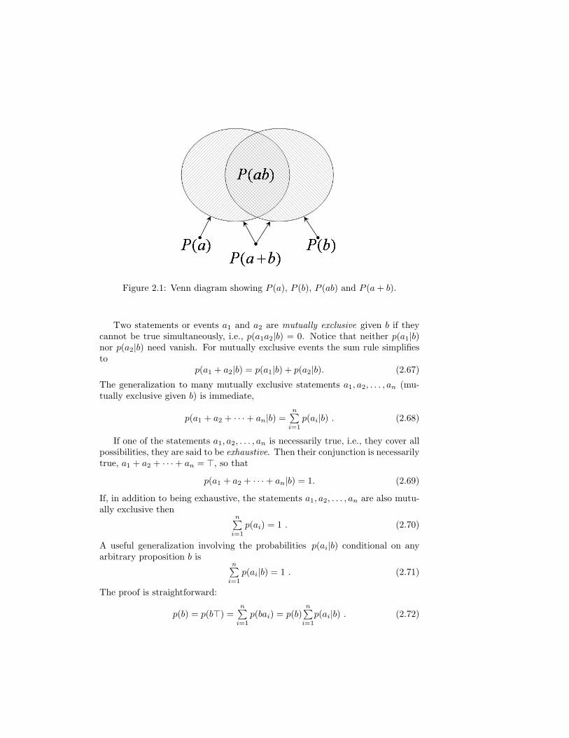
probability as a frequency or as the measure of a set. This is conveyed graphi-cally in a very clear way by Venn diagrams (see fig.2.1).

2.5.3 Independent and mutually exclusive events

In special cases the sum and product rules can be rewritten in various usefulways. Two statements or events a and b are said to be independent if theprobability of one is not altered by information about the truth of the other.More specifically, event a is independent of b (given c) if

p (a|bc) = p (a|c) . (2.65)

For independent events the product rule simplifies to

p(ab|c) = p(a|c)p(b|c) or p(ab) = p(a)p(b) . (2.66)

The symmetry of these expressions implies that p (b|ac) = p (b|c) as well: if a isindependent of b, then b is independent of a.

2.5. SOME REMARKS ON THE SUM AND PRODUCT RULES 21

Figure 2.1: Venn diagram showing P (a), P (b), P (ab) and P (a+ b).

Two statements or events a1 and a2 are mutually exclusive given b if theycannot be true simultaneously, i.e., p(a1a2|b) = 0. Notice that neither p(a1|b)nor p(a2|b) need vanish. For mutually exclusive events the sum rule simplifiesto

p(a1 + a2|b) = p(a1|b) + p(a2|b). (2.67)

The generalization to many mutually exclusive statements a1, a2, . . . , an (mu-tually exclusive given b) is immediate,

p(a1 + a2 + · · ·+ an|b) =n∑i=1

p(ai|b) . (2.68)

If one of the statements a1, a2, . . . , an is necessarily true, i.e., they cover allpossibilities, they are said to be exhaustive. Then their conjunction is necessarilytrue, a1 + a2 + · · ·+ an = >, so that

p(a1 + a2 + · · ·+ an|b) = 1. (2.69)

If, in addition to being exhaustive, the statements a1, a2, . . . , an are also mutu-ally exclusive then

n∑i=1

p(ai) = 1 . (2.70)

A useful generalization involving the probabilities p(ai|b) conditional on anyarbitrary proposition b is

n∑i=1

p(ai|b) = 1 . (2.71)

The proof is straightforward:

p(b) = p(b>) =n∑i=1

p(bai) = p(b)n∑i=1

p(ai|b) . (2.72)


2.5.4 Marginalization

Once we decide that it is legitimate to quantify degrees of belief by real numbersp the problem becomes how do we assign these numbers. The sum and productrules show how we should assign probabilities to some statements once proba-bilities have been assigned to others. Here is an important example of how thisworks.

We want to assign a probability to a particular statement b. Let a1, a2, . . . , anbe mutually exclusive and exhaustive statements and suppose that the proba-bilities of the conjunctions baj are known. We want to calculate p(b) given thejoint probabilities p(baj). The solution is straightforward: sum p(baj) over allajs, use the product rule, and eq.(2.71) to get∑

j

p(baj) = p(b)∑j

p(aj |b) = p(b) . (2.73)

This procedure, called marginalization, is quite useful when we want to eliminateuninteresting variables a so we can concentrate on those variables b that reallymatter to us. The distribution p(b) is referred to as the marginal of the jointdistribution p(ab).

For a second use of formulas such as these suppose that we happen to knowthe conditional probabilities p(b|a). When a is known we can make good infer-ences about b, but what can we tell about b when we are uncertain about theactual value of a? Then we proceed as follows. Use of the sum and productrules gives

p(b) =∑j

p(baj) =∑j

p(b|aj)p(aj) . (2.74)

This is quite reasonable: the probability of b is the probability we would assignif the value of a were precisely known, averaged over all as. The assignment p(b)clearly depends on how uncertain we are about the value of a. In the extremecase when we are totally certain that a takes the particular value ak we havep(aj) = δjk and we recover p(b) = p(b|ak) as expected.

2.6 The expected value

Suppose we know that a quantity x can take values xi with probabilities pi.Sometimes we need an estimate for the quantity x. What should we choose? Itseems reasonable that those values xi that have larger pi should have a dominantcontribution to x. We therefore make the following reasonable choice: Theexpected value of the quantity x is denoted by 〈x〉 and is given by

〈x〉 def=∑i

pi xi . (2.75)

The term ‘expected’ value is not always an appropriate one because 〈x〉 maynot be one of the actually allowed values xi and, therefore, it is not a value we

2.6. THE EXPECTED VALUE 23

would expect. The expected value of a die toss is (1 + · · ·+ 6)/6 = 3.5 which isnot an allowed result.

Using the average 〈x〉 as an estimate for the expected value of x is reason-able, but it is also somewhat arbitrary. Alternative estimates are possible; forexample, one could have chosen the value for which the probability is maximum– this is called the ‘mode’. This raises two questions.

The first question is whether 〈x〉 is a good estimate. If the probability distri-bution is sharply peaked all the values of x that have appreciable probabilitiesare close to each other and to 〈x〉. Then 〈x〉 is a good estimate. But if thedistribution is broad the actual value of x may deviate from 〈x〉 considerably.To describe quantitatively how large this deviation might be we need to describehow broad the probability distribution is.

A convenient measure of the width of the distribution is the root mean square(rms) deviation defined by

∆x def=⟨

(x− 〈x〉)2⟩1/2

. (2.76)

The quantity ∆x is also called the standard deviation, its square (∆x)2 is calledthe variance. For historical reasons it is common to refer to the ‘variance of x’but this is misleading because it suggests that x itself could vary; ∆x refers toour knowledge about x.

If ∆x 〈x〉 then x will not deviate much from 〈x〉 and we expect 〈x〉 to bea good estimate.

The definition of ∆x is somewhat arbitrary. It is dictated both by commonsense and by convenience. Alternatively we could have chosen to define thewidth of the distribution as 〈|x− 〈x〉|〉 or 〈(x− 〈x〉)4〉1/4 but these definitionsare less convenient for calculations.

Now that we have a way of deciding whether 〈x〉 is a good estimate for xwe may raise a second question: Is there such a thing as the “best” estimatefor x? Consider another estimate x′. We expect x′ to be accurate provided thedeviations from it are small, i.e., 〈(x− x′)2〉 is small. The best x′ is that forwhich its variance is a minimum

d

dx′〈(x− x′)2〉

∣∣∣∣x′best

= 0, (2.77)

which implies x′best = 〈x〉. Conclusion: 〈x〉 is the best estimate for x whenby “best” we mean the one with the smallest variance. But other choices arepossible, for example, had we actually decided to minimize the width 〈|x− x′|〉the best estimate would have been the median, x′best = xm, a value such thatProb(x < xm) = Prob(x > xm) = 1/2.

We conclude this section by mentioning two important identities that willbe repeatedly used in what follows. The first is that the average deviation fromthe mean vanishes,

〈x− 〈x〉〉 = 0, (2.78)


because deviations from the mean are just as likely to be positive and negative.The second useful identity is⟨

(x− 〈x〉)2⟩

= 〈x2〉 − 〈x〉2. (2.79)

The proofs are trivial – just use the definition (2.75).

2.7 The binomial distribution

Suppose the probability of a certain event α is p. The probability of α nothappening is 1 − p. Using the theorems discussed earlier we can obtain theprobability that α happens m times in N independent trials. The probabilitythat α happens in the first m trials and not-α or α′ happens in the subsequentN −m trials is, using the product rule for independent events, pm(1− p)N−m.But this is only one particular ordering of the m αs and the N −m α′s. Thereare

N !m!(N −m)!

=(N

m

)(2.80)

such orderings. Therefore, using the sum rule for mutually exclusive events, theprobability of m αs in N independent trials irrespective of the particular orderof αs and αs is

P (m|N, p) =(N

m

)pm(1− p)N−m. (2.81)

This is called the binomial distribution.Using the binomial theorem (hence the name of the distribution) one can

show these probabilities are correctly normalized:

N∑m=0

P (m|N, p) =N∑m=0

(N

m

)pm(1− p)N−m = (p+ (1− p))N = 1. (2.82)

The range of applicability of this distribution is enormous. Whenever trials areindependent of each other (i.e., the outcome of one trial has no influence on theoutcome of another, or alternatively, knowing the outcome of one trial providesus with no information about the possible outcomes of another) the distributionis binomial. Independence is the crucial feature.

The expected number of αs is

〈m〉 =N∑m=0

mP (m|N, p) =N∑m=0

m

(N

m

)pm(1− p)N−m.

This sum over m is complicated. The following elegant trick is useful. Considerthe sum

S(p, q) =N∑m=0

m

(N

m

)pmqN−m,

2.7. THE BINOMIAL DISTRIBUTION 25

where p and q are independent variables. After we calculate S we will replace qby 1− p to obtain the desired result, 〈m〉 = S(p, 1− p). The calculation of S iseasy if we note that mpm = p ∂

∂ppm. Then, using the binomial theorem

S(p, q) = p∂

∂p

N∑m=0

(N

m

)pmqN−m = p

∂

∂p(p+ q)N = Np (p+ q)N−1

.

Replacing q by 1− p we obtain our best estimate for the expected number of αs

〈m〉 = Np . (2.83)

This is the best estimate, but how good is it? To answer we need to calculate∆m. The variance is

(∆m)2 =⟨

(m− 〈m〉)2⟩

= 〈m2〉 − 〈m〉2,

which requires we calculate 〈m2〉,

〈m2〉 =N∑m=0

m2P (m|N, p) =N∑m=0

m2

(N

m

)pm(1− p)N−m.

We can use the same trick we used before to get 〈m〉:

S′(p, q) =N∑m=0

m2

(N

m

)pmqN−m = p

∂

∂p

(p∂

∂p(p+ q)N

).

Therefore,〈m2〉 = (Np)2 +Np(1− p), (2.84)

and the final result for the rms deviation ∆m is

∆m =√Np (1− p). (2.85)

Now we can address the question of how good an estimate 〈m〉 is. Notice that∆m grows with N . This might seem to suggest that our estimate of m getsworse for large N but this is not quite true because 〈m〉 also grows with N . Theratio

∆m〈m〉

=

√(1− p)Np

∝ 1N1/2

, (2.86)

shows that while both the estimate 〈m〉 and its uncertainty ∆m grow with N ,the relative uncertainty decreases.


2.8 Probability vs. frequency: the law of largenumbers

Notice that the “frequency” f = m/N of αs obtained in one N -trial sequence isnot equal to p. For one given fixed value of p, the frequency f can take any oneof the values 0/N, 1/N, 2/N, . . . N/N . What is equal to p is not the frequencyitself but its expected value. Using eq.(2.83),

〈f〉 = 〈mN〉 = p . (2.87)

For large N the distribution is quite narrow and the probability that theobserved frequency of αs differs from p tends to zero as N →∞. Using eq.(2.85),

∆f = ∆(mN

)=

∆mN

=

√p (1− p)

N∝ 1N1/2

. (2.88)

The same ideas are more precisely conveyed by a theorem due to Bernoulliknown as the ‘weak law of large numbers’. A simple proof of the theoreminvolves an inequality due to Tchebyshev. Let ρ (x) dx be the probability thata variable X lies in the range between x and x+ dx,

P (x < X < x+ dx) = ρ (x) dx.

The variance of X satisfies

(∆x)2 =∫

(x− 〈x〉)2ρ (x) dx ≥

∫|x−〈x〉|≥ε

(x− 〈x〉)2ρ (x) dx ,

where ε is an arbitrary constant. Replacing (x− 〈x〉)2 by its least value ε2 gives

(∆x)2 ≥ ε2

∫|x−〈x〉|≥ε

ρ (x) dx = ε2 P (|x− 〈x〉| ≥ ε) ,

which is Tchebyshev’s inequality,

P (|x− 〈x〉| ≥ ε) ≤(

∆xε

)2

. (2.89)

Next we prove Bernoulli’s theorem, the weak law of large numbers. Firsta special case. Let p be the probability of outcome α in an experiment E,P (α|E) = p. In a sequence of N independent repetitions of E the probabilityof m outcomes α is binomial. Substituting

〈f〉 = p and (∆f)2 =p (1− p)

N

into Tchebyshev’s inequality we get Bernoulli’s theorem,

P(|f − p| ≥ ε |EN

)≤ p (1− p)

Nε2. (2.90)

2.8. THE LAW OF LARGE NUMBERS 27

Therefore, the probability that the observed frequency f is appreciably differentfrom p tends to zero as N →∞. Or equivalently: for any small ε, the probabilitythat the observed frequency f = m/N lies in the interval between p− ε/2 andp+ ε/2 tends to unity as N →∞.

In the mathematical/statistical literature this result is commonly stated inthe form

f −→ p in probability. (2.91)

The qualifying words ‘in probability’ are crucial: we are not saying that theobserved f tends to p for large N . What vanishes for large N is not the differencef−p itself, but rather the probability that |f − p| is larger than a certain (small)amount.

Thus, probabilities and frequencies are not the same thing but they arerelated to each other. Since 〈f〉 = p, one might perhaps be tempted to definethe probability p in terms of the expected frequency 〈f〉, but this does not workeither. The problem is that the notion of expected value already presupposesthat the concept of probability has been defined previously. The definition of aprobability in terms of expected values is unsatisfactory because it is circular.

The law of large numbers is easily generalized beyond the binomial distribu-tion. Consider the average

x =1N

N∑r=1

xr , (2.92)

where x1, . . . , xN are N independent variables with the same mean 〈xr〉 = µ andvariance var(xr) = (∆xr)

2 = σ2. (In the previous discussion leading to eq.(2.90)each variable xr is either 1 or 0 according to whether outcome α happens or notin the rth repetition of experiment E.)

To apply Tchebyshev’s inequality, eq.(2.89), we need the mean and the vari-ance of x. Clearly,

〈x〉 =1N

N∑r=1〈xr〉 =

1NNµ = µ . (2.93)

Furthermore, since the xr are independent, their variances are additive. Forexample,

var(x1 + x2) = var(x1) + var(x2) . (2.94)

(Prove it.) Therefore,

var(x) =N∑r=1

var(xrN

) = N( σN

)2

=σ2

N. (2.95)

Tchebyshev’s inequality now gives,

P(|x− µ| ≥ ε|EN

)≤ σ2

Nε2(2.96)

so that for any ε > 0

limN→∞

P(|x− µ| ≥ ε|EN

)= 0 or lim

N→∞P(|x− µ| ≤ ε|EN

)= 1 , (2.97)


orx −→ µ in probability. (2.98)

Again, what vanishes for large N is not the difference x − µ itself, but ratherthe probability that |x− µ| is larger than any given small amount.

2.9 The Gaussian distribution

The Gaussian distribution is quite remarkable, it applies to a wide variety ofproblems such as the distribution of errors affecting experimental data, thedistribution of velocities of molecules in gases and liquids, the distribution offluctuations of thermodynamical quantities, and so on and on. One suspectsthat a deeply fundamental reason must exist for its wide applicability. Somehowthe Gaussian distribution manages to codify the information that happens tobe relevant for prediction in a wide variety of problems. The Central LimitTheorem discussed below provides an explanation.

2.9.1 The de Moivre-Laplace theorem

The Gaussian distribution turns out to be a special case of the binomial distri-bution. It applies to situations when the number N of trials and the expectednumber of αs, 〈m〉 = Np, are both very large (i.e., N large, p not too small).

To find an analytical expression for the Gaussian distribution we note thatwhen N is large the binomial distribution,

P (m|N, p) =N !

m!(N −m)!pm(1− p)N−m,

is very sharply peaked: P (m|N, p) is essentially zero unless m is very close to〈m〉 = Np. This suggests that to find a good approximation for P we need topay special attention to a very small range of m and this can be done followingthe usual approach of a Taylor expansion. A problem is immediately apparent:if a small change in m produces a small change in P then we only need to keepthe first few terms, but in our case P is a very sharp function. To reproducethis kind of behavior we need a huge number of terms in the series expansionwhich is impractical. Having diagnosed the problem one can easily find a cure:instead of finding a Taylor expansion for the rapidly varying P , one finds anexpansion for log P which varies much more smoothly.

Let us therefore expand log P about its maximum at m0, the location ofwhich is at this point still unknown. The first few terms are

logP = logP |m0+d logPdm

∣∣∣∣m0

(m−m0) +12d2 logPdm2

∣∣∣∣m0

(m−m0)2 + . . . ,

where

logP = logN !− logm!− log (N −m)! +m log p+ (N −m) log (1− p) .

2.9. THE GAUSSIAN DISTRIBUTION 29

What is a derivative with respect to an integer? For large m the function logm!varies so slowly (relative to the huge value of logm! itself) that we may considerm to be a continuous variable. Then

d logm!dm

≈ logm!− log (m− 1)!1

= logm!

(m− 1)!= logm . (2.99)

Integrating one obtains a very useful approximation – called the Stirling ap-proximation – for the logarithm of a large factorial

logm! ≈∫ m

0

log x dx = (x log x− x)|m0 = m log m−m.

A somewhat better expression which includes the next term in the Stirling ex-pansion is

logm! ≈ m logm−m+12

log 2πm+ . . . (2.100)

Notice that the third term is much smaller than the first two; the first twoterms are of order m while the last is of order logm. For m = 1023, logm isonly 55.3.

The derivatives in the Taylor expansion are

d logPdm

= − logm+ log (n−m) + log p− log (1− p) = logp(N −m)m(1− p)

,

andd2 logPdm2

= − 1m− 1N −m

=−N

m(N −m).

To find the value m0 where P is maximum set d logP/dm = 0. This givesm0 = Np = 〈m〉, and substituting into the second derivative of logP we get

d2 logPdm2

∣∣∣∣〈m〉

= − 1Np (1− p)

= − 1(∆m)2 .

Therefore

logP = logP (〈m〉)− (m− 〈m〉)2

2 (∆m)2 + . . .

or

P (m) = P (〈m〉) exp

[− (m− 〈m〉)2

2 (∆m)2

].

The remaining unknown constant P (〈m〉) can be evaluated by requiring thatthe distribution P (m) be properly normalized, that is

1 =N∑m=0

P (m) ≈∫ N

0

P (x) dx ≈∫ ∞−∞

P (x) dx.


Using ∫ ∞−∞

e−αx2dx =

√π

α,

we get

P (〈m〉) =1√

2π (∆m)2.

Thus, the expression for the Gaussian distribution with mean 〈m〉 and rmsdeviation ∆m is

P (m) =1√

2π (∆m)2exp

[− (m− 〈m〉)2

2 (∆m)2

]. (2.101)

It can be rewritten as a probability for the frequency f = m/N using 〈m〉 = Np

and (∆m)2 = Np (1− p). The probability that f lies in the small range df =1/N is

p(f)df =1√

2πσ2N

exp

[− (f − p)2

2σ2N

]df , (2.102)

where σ2N = p(1− p)/N .

To appreciate the significance of the theorem consider a macroscopic variablex built up by adding a large number of small contributions, x =

∑Nn=1 ξn, where

the ξn are statistically independent. We assume that each ξn takes the value εwith probability p, and the value 0 with probability 1−p. Then the probabilitythat x takes the value mε is given by the binomial distribution P (m|N, p). Forlarge N the probability that x lies in the small range mε± dx/2 where dx = εis

p(x)dx =1√

2π (∆x)2exp

[− (x− 〈x〉)2

2 (∆x)2

]dx , (2.103)

where 〈x〉 = Npε and (∆x)2 = Np(1 − p)ε2. Thus, the Gaussian distributionarises whenever we have a quantity that is the result of adding a large numberof small independent contributions. The derivation above assumes that themicroscopic contributions are discrete (binomial, either 0 or ε), and identicallydistributed but, as shown in the next section, both of these conditions can berelaxed.

2.9.2 The Central Limit Theorem

Consider the average

x =1N

N∑r=1

xr , (2.104)

2.9. THE GAUSSIAN DISTRIBUTION 31

of N independent variables x1, . . . , xN . Our goal is to calculate the probabilityof x in the limit of large N . Let pr(xr) be the probability distribution for therth variable with

〈xr〉 = µr and (∆xr)2 = σ2

r . (2.105)

The probability density for x is given by the integral

P (x) =∫dx1 . . . dxN p1(x1) . . . pN (xN ) δ

(x− 1

N

N∑r=1

xr

). (2.106)

(This is just an exercise in the sum and product rules.) To calculate P (x)introduce the averages

µdef=

1N

N∑r=1

µr and σ2 def=1N

N∑r=1

σ2r , (2.107)

and consider the distribution for the variable x− µ which is Pr(x− µ) = P (x).It’s Fourier transform,

F (k) =∫dx Pr(x− µ)eik(x−µ) =

∫dxP (x)eik(x−µ)

=∫dx1 . . . dxN p1(x1) . . . pN (xN ) exp

[ik

N

N∑r=1

(xr − µr)],

can be rearranged into a product

F (k) =[∫

dx1 p1(x1)eikN (x1−µ1)

]. . .

[∫dxN pN (xN )ei

kN (xN−µN )

]. (2.108)

The Fourier transform f(k) of a distribution p(ξ) has many interesting anduseful properties. For example,

f(k) =∫dξ p(ξ)eikξ =

⟨eikξ

⟩, (2.109)

and the series expansion of the exponential gives

f(k) =⟨ ∞∑n=0

(ikξ)n

n!

⟩=∞∑n=0

(ik)n

n!〈ξn〉 . (2.110)

In words, the coefficients of the Taylor expansion of f(k) give all the momentsof p(ξ). The Fourier transform f(k) is called the moment generating functionand also the characteristic function of the distribution.

Going back to our calculation of P (x), eq.(2.106), its Fourier transform,eq.(2.108) is,

F (k) =N∏r=1

fr(k

N) , (2.111)


where

fr(k

N) =

∫dxr pr(xr)ei

kN (xr−µr)

= 1 + ik

N〈xr − µr〉 −

k2

2N2

⟨(xr − µr)2

⟩+ . . .

= 1− k2σ2r

2N2+O

(k3

N3

). (2.112)

For a sufficiently large N this can be written as

fr(k

N) −→ exp

(−k

2σ2r

2N2

). (2.113)

so that

F (k) = exp(− k2

2N2

N∑r=1

σ2r

)= exp

(−k

2σ2

2N

). (2.114)

Finally, taking the inverse Fourier transform, we obtain the desired result, whichis called the central limit theorem

Pr(x− µ) = P (x) =1√

2πσ2/Nexp

(− (x− µ)2

2σ2/N

). (2.115)

To conclude we comment on its significance. We have shown that almostindependently of the form of the distributions pr (xr) the distribution of theaverage x is Gaussian centered at µ with standard deviation σ2/N . Not onlythe pr (xr) need not be binomial, they do not even have to be equal to each other.This helps to explain the widespread applicability of the Gaussian distribution:it applies to almost any ‘macro-variable’ (such as x) that results from adding alarge number of independent ‘micro-variables’ (such as xr/N).

But there are restrictions; although very common, Gaussian distributions donot obtain always. A careful look at the derivation above shows the crucial stepwas taken in eqs.(2.112) and (2.114) where we neglected the contributions of thethird and higher moments. Earlier we mentioned that the success of Gaussiandistributions is due to the fact that they codify the information that happens tobe relevant to the particular phenomenon under consideration. Now we see whatthat relevant information might be: it is contained in the first two moments,the mean and the variance – Gaussian distributions are successful when thirdand higher moments are irrelevant. (This can be stated more precisely in termsas the so-called Lyapunov condition.)

Later we shall approach this same problem from the point of view of themethod of maximum entropy and there we will show that, indeed, the Gaussiandistribution can be derived as the distribution that codifies information aboutthe mean and the variance while remaining maximally ignorant about everythingelse.

2.10. UPDATING PROBABILITIES: BAYES’ RULE 33

2.10 Updating probabilities: Bayes’ rule

Now that we have solved the problem of how to represent a state of knowledgeas a consistent web of interconnected beliefs we can address the problem ofupdating from one consistent web of beliefs to another when new informationbecomes available. We will only consider those special situations where theinformation to be processed is in the form of data.

Specifically the problem is to update our beliefs about θ (either a singleparameter or many) on the basis of data x (either a single number or several)and of a known relation between θ and x. The updating consists of replacing theprior probability distribution p(θ) that represents our beliefs before the data isprocessed, by a posterior distribution pnew(θ) that applies after the data hasbeen processed.

2.10.1 Formulating the problem

We must first describe the state of our knowledge before the data has beencollected or, if the data has already been collected, before we have taken it intoaccount. At this stage of the game not only we do not know θ, we do not knowx either. As mentioned above, in order to infer θ from x we must also know howthese two quantities are related to each other. Without this information onecannot proceed further. Fortunately we usually know enough about the physicsof an experiment that if θ were known we would have a fairly good idea of whatvalues of x to expect. For example, given a value θ for the charge of the electron,we can calculate the velocity x of an oil drop in Millikan’s experiment, addsome uncertainty in the form of Gaussian noise and we have a very reasonableestimate of the conditional distribution p(x|θ). The distribution p(x|θ) is calledthe sampling distribution and also (less appropriately) the likelihood. We willassume it is known.

We should emphasize that the crucial information about how x is related toθ is contained in the functional form of the distribution p(x|θ) – say, whetherit is a Gaussian or a Cauchy distribution – and not in the actual values of thearguments x and θ which are, at this point, still unknown.

Thus, to describe the web of prior beliefs we must know the prior p(θ) andalso the sampling distribution p(x|θ). This means that we must know the fulljoint distribution,

p(θ, x) = p(θ)p(x|θ) . (2.116)

This is very important: we must be clear about what we are talking about. Therelevant universe of discourse is neither the space Θ of possible parameters θ noris it the space X of possible data x. It is rather the product space Θ × X andthe probability distributions that concern us are the joint distributions p(θ, x).

Next we collect data: the observed value turns out to be X. Our goal isto use this information to update to a web of posterior beliefs represented bya new joint distribution pnew(θ, x). How shall we choose pnew(θ, x)? The newdata tells us that the value of x is now known to be X. Therefore, the new web


of beliefs must be such that

pnew(x) =∫dθ pnew(θ, x) = δ(x−X) . (2.117)

(For simplicity we have here assumed that x is a continuous variable; had x beendiscrete Dirac δs would be replaced by Kronecker δs.) This is all we know butit is not sufficient to determine pnew(θ, x). Apart from the general requirementthat the new web of beliefs must be internally consistent there is nothing in anyof our previous considerations that induces us to prefer one consistent web overanother. A new principle is needed.

2.10.2 Minimal updating: Bayes’ rule

The basic updating strategy that we adopt below reflects the conviction thatwhat we have learned in the past, the prior knowledge, is a valuable resourcethat should not be squandered. Prior beliefs should be revised only when this isdemanded by the new information; the new web of beliefs should coincide withthe old one as much as possible. We propose to adopt the following

Principle of Minimal Updating (PMU): The web of beliefs needs to berevised only to the extent required by the new data.

This seems so reasonable and natural that an explicit statement may seemsuperfluous. The important point, however, is that it is not logically necessary.We could update in many other ways that preserve both internal consistencyand consistency with the new information.

As we saw above the new data, eq.(2.117), does not fully determine the jointdistribution

pnew(θ, x) = pnew(x)pnew(θ|x) = δ(x−X)pnew(θ|x) . (2.118)

All distributions of the form

pnew(θ, x) = δ(x−X)pnew(θ|X) , (2.119)

where pnew(θ|X) remains arbitrary is compatible with the newly acquired data.We still need to assign pnew(θ|X). It is at this point that we invoke the PMU.We stipulate that no further revision is needed and set

pnew(θ|X) = pold(θ|X) = p(θ|X) . (2.120)

Therefore, the web of posterior beliefs is described by

pnew(θ, x) = δ(x−X)p(θ|X) . (2.121)

The posterior probability pnew(θ) is

pnew(θ) =∫dx pnew(θ, x) =

∫dx δ(x−X)p(θ|X) , (2.122)


or,

pnew(θ) = p(θ|X) . (2.123)

In words, the posterior probability equals the prior conditional probability ofθ given X. This result, known as Bayes’ rule, is extremely reasonable: wemaintain those beliefs about θ that are consistent with the data values X thatturned out to be true. Data values that were not observed are discarded becausethey are now known to be false. ‘Maintain’ is the key word: it reflects the PMUin action.

Using the product rule

p(θ,X) = p(θ)p(X|θ) = p(X)p(θ|X) , (2.124)

Bayes’ rule can be written as

pnew(θ) = p(θ)p(X|θ)p(X)

. (2.125)

Remark: Bayes’ rule is usually written in the form

p(θ|X) = p(θ)p(X|θ)p(X)

, (2.126)

and called Bayes’ theorem. This formula is very simple; perhaps it is too simple.It is just a restatement of the product rule, eq.(2.124), and therefore it is asimple consequence of the internal consistency of the prior web of beliefs. Thedrawback of this formula is that the left hand side is not the posterior butrather the prior conditional probability; it obscures the fact that an additionalprinciple – the PMU – was needed for updating.

The interpretation of Bayes’ rule is straightforward: according to eq.(2.125)the posterior distribution pnew(θ) gives preference to those values of θ that werepreviously preferred as described by the prior p(θ), but this is now modulatedby the likelihood factor p(X|θ) in such a way as to enhance our preference forvalues of θ that make the data more likely, less surprising. The factor in thedenominator p(X) which is the prior probability of the data is given by

p(X) =∫p(θ)p(X|θ) dθ , (2.127)

and plays the role of a normalization constant for the posterior distributionpnew(θ). It does not help to discriminate one value of θ from another because itaffects all values of θ equally and is therefore not important except, as we shallsee later in this chapter, in problems of model selection.

Neither the rule, eq.(2.123), nor the theorem, eq.(2.126), was ever actuallywritten down by Bayes. The person who first explicitly stated the theorem and,more importantly, who first realized its deep significance was Laplace.


Example: is there life on Mars?

Suppose we are interested in whether there is life on Mars or not. How isthe probability that there is life on Mars altered by new data indicating thepresence of water on Mars. Let θ =‘There is life on Mars’. The prior informationincludes the fact I = ‘All known life forms require water’. The new data is thatX = ‘There is water on Mars’. Let us look at Bayes’ rule. We can’t say muchabout p (X|I) but whatever its value it is definitely less than 1. On the otherhand p (X|θI) ≈ 1. Therefore the factor multiplying the prior is larger than1. Our belief in the truth of θ is strengthened by the new data X. This isjust common sense, but notice that this kind of probabilistic reasoning cannotbe carried out if one adheres to a strictly frequentist interpretation – there isno set of trials. The name ‘Bayesian probabilities’ given to ‘degrees of belief’originates in the fact that it is only under this interpretation that the full powerof Bayes’ rule can be exploited.

Example: testing positive for a rare disease

Suppose you are tested for a disease, say cancer, and the test turns out to bepositive. Suppose further that the test is said to be 99% accurate. Should youpanic? It may be wise to proceed with caution.

One should start by explaining that ‘99% accurate’ means that when the testis applied to people known to have cancer the result is positive 99% of the time,and when applied to people known to be healthy, the result is negative 99% ofthe time. We express this accuracy as p(y|c) = A = 0.99 and p(n|c) = A = 0.99(y and n stand for ‘positive’ and ‘negative’, c and c stand for ‘cancer’ or ‘nocancer’). There is a 1% probability of false positives, p(y|c) = 1−A, and a 1%probability of false negatives, p(n|c) = 1−A.

On the other hand, what we really want to know is pnew(c) = p(c|y), theprobability of having cancer given that you tested positive. This is not thesame as the probability of testing positive given that you have cancer, p(y|c);the two probabilities are not the same thing! So there might be some hope. Theconnection between what we want, p(c|y), and what we know, p(y|c), is givenby Bayes’ theorem,

p(c|y) =p(c)p(y|c)p(y)

.

An important virtue of Bayes’ rule is that it doesn’t just tell you how toprocess information; it also tells you what information you should seek. In thiscase one should find p(c), the probability of having cancer irrespective of beingtested positive or negative. Suppose you inquire and find that the incidence ofcancer in the general population is 1%; this means that p(c) = 0.01. Thus,

p(c|y) =p(c)Ap(y)

One also needs to know p(y), the probability of the test being positive irre-


spective of whether the person has cancer or not. To obtain p(y) use

p(c|y) =p(c)p(y|c)p(y)

=(1− p(c)) (1−A)

p(y),

and p(c|y) + p(c|y) = 1 which leads to our final answer

p(c|y) =p(c)A

p(c)A+ (1− p(c)) (1−A). (2.128)

For an accuracy A = 0.99 and an incidence p(c) = 0.01 we get p(c|y) = 50%which is not nearly as bad as one might have originally feared. Should onedismiss the information provided by the test as misleading? No. Note that theprobability of having cancer prior to the test was 1% and on learning the testresult this was raised all the way up to 50%. Note also that when the diseaseis really rare, p(c) → 0, we still get p(c|y) → 0 even when the test is quiteaccurate. This means that for rare diseases most positive tests turn out to befalse positives.

We conclude that both the prior and the data contain important information;neither should be neglected.Remark: The previous discussion illustrates a mistake that is common in verbaldiscussions: if h denotes a hypothesis and e is some evidence, it is quite obviousthat we should not confuse p(e|h) with p(h|e). However, when expressed verballythe distinction is not nearly as obvious. For example, in a criminal trial jurorsmight be told that if the defendant were guilty (the hypothesis) the probabilityof some observed evidence would be large, and the jurors might easily be misledinto concluding that given the evidence the probability is high that the defendantis guilty. Lawyers call this the prosecutor’s fallacy.

Example: uncertain data

As before we want to update from a prior joint distribution p(θ, x) = p(x)p(θ|x)to a posterior joint distribution pnew(θ, x) = pnew(x)pnew(θ|x) when informationbecomes available. When the information is data X that precisely fixes the valueof x, we impose that pnew(x) = δ(x − X). The remaining unknown pnew(θ|x)is determined by invoking the PMU: no further updating is needed. This fixespnew(θ|x) to be the old p(θ|x) and yields Bayes’ rule.

It may happen, however, that there is a measurement error. The data Xthat was actually observed does not constrain the value of x completely. To beexplicit let us assume that the remaining uncertainty in x is well understood:the observation X constrains our beliefs about x to a distribution PX(x) thathappens to be known. PX(x) could, for example, be a Gaussian distributioncentered at X, with some known standard deviation σ.

This information is incorporated into the posterior distribution, pnew(θ, x) =pnew(x)pnew(θ|x), by imposing that pnew(x) = PX(x). The remaining condi-tional distribution is, as before, determined by invoking the PMU,

pnew(θ|x) = pold(θ|x) = p(θ|x) , (2.129)


and therefore, the joint posterior is

pnew(θ, x) = PX(x)p(θ|x) . (2.130)

Marginalizing over the uncertain x yields the new posterior for θ,

pnew(θ) =∫dxPX(x)p(θ|x) . (2.131)

This generalization of Bayes’ rule is sometimes called Jeffrey’s conditionalizationrule.

Incidentally, this is an example of updating that shows that it is not alwaysthe case that information comes purely in the form of data X. In the derivationabove there clearly is some information in the observed value X and some in-formation in the particular functional form of the distribution PX(x), whetherit is a Gaussian or some other distribution.

The common element in our previous derivation of Bayes’ rule and in thepresent derivation of Jeffrey’s rule is that in both cases the information beingprocessed is a constraint on the allowed posterior marginal distributions pnew(x).Later we shall see (chapter 5) how the updating rules can be generalized stillfurther to apply to even more general constraints.

2.10.3 Multiple experiments, sequential updating

The problem here is to update our beliefs about θ on the basis of data x1, x2, . . . , xnobtained in a sequence of experiments. The relations between θ and the vari-ables xi are given through known sampling distributions. We will assume thatthe experiments are independent but they need not be identical. When the ex-periments are not independent it is more appropriate to refer to them as beingperformed is a single more complex experiment the outcome of which is a set ofnumbers x1, . . . , xn.

For simplicity we deal with just two identical experiments. The prior webof beliefs is described by the joint distribution,

p(x1, x2, θ) = p(θ) p(x1|θ)p(x2|θ) = p(x1)p(θ|x1)p(x2|θ) , (2.132)

where we have used independence, p(x2|θ, x1) = p(x2|θ).The first experiment yields the data x1 = X1. Bayes’ rule gives the updated

distribution for θ as

p1(θ) = p(θ|X1) = p(θ)p(X1|θ)p(X1)

. (2.133)

The second experiment yields the data x2 = X2 and requires a second applica-tion of Bayes’ rule. The posterior p1(θ) in eq.(2.133) now plays the role of theprior and the new posterior distribution for θ is

p12(θ) = p1(θ|X2) = p1(θ)p(X2|θ)p1(X2)

. (2.134)


We have explicitly followed the update from p(θ) to p1(θ) to p12(θ). It isstraightforward to show that the same result is obtained if the data from bothexperiments were processed simultaneously,

p12(θ) = p(θ|X1, X2) = p(θ)p(X1, X2|θ)p(X1, X2)

. (2.135)

Indeed, using eq.(2.132) and (2.133), this last equation can be rewritten as

p12(θ) = p(θ)p(X1|θ)p(X1)

p(X2|θ)p(X2|X1)

= p1(θ)p(X2|θ)p(X2|X1)

, (2.136)

and it remains to show that p(X2|X1) = p1(X2). This last step is straightfor-ward; use eq.(2.134) and (2.133):

p1(X2) =∫p1(θ)p(X2|θ)dθ =

∫p(θ)

p(X1|θ)p(X1)

p(X2|θ)dθ

=∫ p(X1, X2, θ)

p(X1)dθ = p(X2|X1) . (2.137)

From the symmetry of eq.(2.135) it is clear that the same posterior p12(θ)is obtained irrespective of the order that the data X1 and X2 are processed.The commutativity of Bayesian updating follows from the special circumstancethat the information conveyed by one experiment does not revise or renderobsolete the information conveyed by the other experiment. As we generalize ourmethods of inference for processing other kinds of information that do interferewith each other (and therefore one may render the other obsolete) we shouldnot expect, much less demand, that commutativity will continue to hold.

2.10.4 Remarks on priors

Let us return to the question of the extent to which probabilities incorporatesubjective and objective elements. We have seen that Bayes’ rule allows usto update from prior to posterior distributions. The posterior distributionsincorporate the presumably objective information contained in the data pluswhatever earlier beliefs had been codified into the prior. To the extent that theBayes updating rule is itself unique one can claim that the posterior is “moreobjective” than the prior. As we update more and more we should expect thatour probabilities should reflect more and more the input data and less and lessthe original subjective prior distribution. In other words, some subjectivityis unavoidable at the beginning of an inference chain, but it can be graduallysuppressed as more and more information is processed.

The problem of choosing the first prior in the inference chain is a difficultone. We will tackle it in several different ways. Later in this chapter, as weintroduce some elementary notions of data analysis, we will address it in thestandard way: just make a “reasonable” guess – whatever that might mean.With experience and intuition this seems to work well. But when addressing


new problems we have neither experience nor intuition and guessing is risky. Wewould like to develop more systematic ways to proceed. Indeed it can be shownthat certain types of prior information (for example, symmetries and/or otherconstraints) can be objectively translated into a prior once we have developedthe appropriate tools – entropy and geometry. (See e.g. [Caticha Preuss 04]and references therein.)

Our immediate goal here is, first, to remark on the dangerous consequences ofextreme degrees of belief, and then to prove our previous intuitive assertion thatthe accumulation of data will swamp the original prior and render it irrelevant.

Dangerous extremes: the prejudiced mind

The consistency of Bayes’ rule can be checked for the extreme cases of certaintyand impossibility: Let B describe any background information. If p (θ|B) = 1,then θB = B and p(X|θB) = p(X|B), so that Bayes’ rule gives

pnew(θ|B) = p(θ|B)p(X|θB)p(X|B)

= 1 . (2.138)

A similar argument can be carried through in the case of impossibility: Ifp (θ|B) = 0, then pnew (θ|B) = 0. Conclusion: if we are absolutely certainabout the truth of θ, acquiring data X will have absolutely no effect on ouropinions; the new data is worthless.

This should serve as a warning to the dangers of erroneously assigning aprobability of 1 or of 0: since no amount of data could sway us from our priorbeliefs we may decide we did not need to collect the data in the first place. Ifyou are absolutely sure that Jupiter has no moons, you may either decide thatit is not necessary to look through the telescope, or, if you do look and yousee some little bright spots, you will probably decide the spots are mere opticalillusions. Extreme degrees of belief are dangerous: a truly prejudiced mind doesnot, and indeed, cannot question its own beliefs.

Lots of data overwhelms the prior

As more and more data is accumulated according to the sequential updatingdescribed earlier one would expect that the continuous inflow of informationwill eventually render irrelevant whatever prior information we might have hadat the start. This is indeed the case: unless we have assigned a pathologicalprior – all we need is a prior that is smooth where the likelihood is large – aftera large number of experiments the posterior becomes essentially independent ofthe prior.

Consider N independent repetitions of a certain experiment E that yield thedata X = X1 . . . XN. The corresponding likelihood is

p(X|θ) =N∏r=1

p(Xr|θ) , (2.139)


and the posterior distribution pnew(θ) is

p(θ|X) =p(θ)p(X)

p(X|θ) =p(θ)p(X)

N∏r=1

p(Xr|θ) . (2.140)

To investigate the extent to which the data X supports the particular valueθ1 rather than any other value θ2 it is convenient to study the ratio

p(θ1|X)p(θ2|X)

=p(θ1)p(θ2)

R(X) , (2.141)

where we introduce the likelihood ratios,

R(X) def=N∏r=1

Rr(Xr) and Rr(Xr)def=

p(Xr|θ1)p(Xr|θ2)

. (2.142)

We want to prove the following theorem: Barring two trivial exceptions, for anyarbitrarily large positive Λ, we have

limN→∞

P (R(X) > Λ|θ1) = 1 (2.143)

or, in other words,

given θ1, R(X) −→∞ in probability. (2.144)

The significance of the theorem is that as data accumulates a rational personbecomes more and more convinced of the truth – in this case the true value isθ1 – and this happens essentially irrespective of the prior p(θ).

The theorem fails in two cases: first, when the prior p(θ1) vanishes, inwhich case probabilities conditional on θ1 are meaningless, and second, whenp(Xr|θ1) = p(Xr|θ2) for all Xr which describes an experiment E that is flawedbecause it cannot distinguish between θ1 and θ2.

The proof of the theorem is an application of the weak law of large numbers.Consider the quantity

1N

logR(X) =1N

N∑r=1

logRr(Xr) (2.145)

Since the variables logRr(Xr) are independent, eq.(2.97) gives

limN→∞

P

(∣∣∣∣ 1N

logR(X)−K(θ1, θ2)∣∣∣∣ ≤ ε|θ1

)= 1 (2.146)

where ε is any small positive number and

K(θ1, θ2) =⟨

1N

logR(X)|θ1

⟩=∑Xr

p(Xr|θ1) logRr(Xr) . (2.147)


In other words,

given θ1, eN(K−ε) ≤ R(X) ≤ eN(K+ε) in probability. (2.148)

In Chapter 4 we will prove that K(θ1, θ2) ≥ 0 with equality if and only if the twodistributions p(Xr|θ1) and p(Xr|θ2) are identical, which is precisely the secondof the two trivial exceptions we explicitly avoid. Thus K(θ1, θ2) > 0, and thisconcludes the proof.

We see here the first appearance of a quantity,

K(θ1, θ2) = +∑Xr

p(Xr|θ1) logp(Xr|θ1)p(Xr|θ2)

, (2.149)

that will prove to be central in later discussions. When multiplied by −1,the quantity −K(θ1, θ2) is called the relative entropy,2 that is the entropy ofp(Xr|θ1) relative to p(Xr|θ2). It can be interpreted as a measure of the extentthat the distribution p(Xr|θ1) can be distinguished from p(Xr|θ2).

2.11 Examples from data analysis

To illustrate the use of Bayes’ theorem as a tool to process information whenthe information is in the form of data we consider some elementary examplesfrom the field of data analysis. (For detailed treatments that are friendly tophysicists see e.g. [Sivia Skilling 06, Gregory 05].)

2.11.1 Parameter estimation

Suppose the probability for the quantity x depends on certain parameters θ,p = p(x|θ). Although most of the discussion here can be carried out for anarbitrary function p it is best to be specific and focus on the important case ofa Gaussian distribution,

p(x|µ, σ) =1√

2πσ2exp

(− (x− µ)2

2σ2

). (2.150)

The objective is to estimate the parameters θ = (µ, σ) on the basis of a set ofdata X = X1, . . . XN. We assume the measurements are statistically inde-pendent of each other and use Bayes’ theorem to get

p(µ, σ|X) =p(µ, σ)p (X)

N∏i=1

p(Xi|µ, σ) . (2.151)

Independence is important in practice because it leads to considerable practicalsimplifications but it is not essential: instead of N independent measurements

2Other names include relative information, directed divergence, and Kullback-Leibler dis-tance.

2.11. EXAMPLES FROM DATA ANALYSIS 43

each providing a single datum we would have a single complex experiment thatprovides N non-independent data.

Looking at eq.(2.151) we see that a more precise formulation of the sameproblem is the following. We want to estimate certain parameters θ, in our caseµ and σ, from repeated measurements of the quantity x on the basis of severalpieces of information. The most obvious is

1. The information contained in the actual values of the collected data X.

Almost equally obvious (at least to those who are comfortable with the Bayesianinterpretation of probabilities) is

2. The information about the parameters that is codified into the prior dis-tribution p(θ).

Where and how this prior information was obtained is not relevant at this point;it could have resulted from previous experiments, or from other backgroundknowledge about the problem. The only relevant part is whatever ended upbeing distilled into p(θ).

The last piece of information is not always explicitly recognized; it is

3. The information that is codified into the functional form of the ‘sampling’distribution p(X|θ).

If we are to estimate parameters θ on the basis of measurements of a quantityx it is clear that we must know how θ and x are related to each other. Noticethat item 3 refers to the functional form – whether the distribution is Gaussianas opposed to Poisson or binomial or something else – and not to the actualvalues of the data X which is what is taken into account in item 1. The natureof the relation in p(X|θ) is in general statistical but it could also be completelydeterministic. For example, when X is a known function of θ, say X = f(θ), wehave p(X|θ) = δ [X − f(θ)]. In this latter case there is no need for Bayes’ rule.

Eq. (2.151) is rewritten as

p(µ, σ|X) =p(µ, σ)p (X)

1

(2πσ2)N/2exp

[−

N∑i=1

(Xi − µ)2

2σ2

](2.152)

Introducing the sample average X and sample variance s2,

X =1N

N∑i=1

Xi and s2 =1N

N∑i=1

(Xi − X

)2, (2.153)

eq.(2.152) becomes

p(µ, σ|X) =p(µ, σ)p (X)

1

(2πσ2)N/2exp

[−(µ− X

)2 + s2

2σ2/N

]. (2.154)


It is interesting that the data appears here only in the particular combinationin eq.(2.153) – different sets of data characterized by the same X and s2 lead tothe same inference about µ and σ. (As discussed earlier the factor p (X) is notrelevant here since it can be absorbed into the normalization of the posteriorp(µ, σ|X).)

Eq. (2.154) incorporates the information described in items 1 and 3 above.The prior distribution, item 2, remains to be specified. Let us start by consid-ering the simple case where the value of σ is actually known. Then p(µ, σ) =p(µ)δ(σ − σ0) and the goal is to estimate µ. Bayes’ theorem is now written as

p(µ|X) =p(µ)p (X)

1

(2πσ20)N/2

exp

[−

N∑i=1

(Xi − µ)2

2σ20

](2.155)

=p(µ)p (X)

1

(2πσ20)N/2

exp

[−(µ− X

)2 + s2

2σ20/N

]

∝ p(µ) exp

[−(µ− X

)22σ2

0/N

]. (2.156)

Suppose further that we know nothing about µ; it could have any value. Thisstate of extreme ignorance is represented by a very broad distribution that wetake as essentially uniform within some large range; µ is just as likely to have onevalue as another. For p(µ) ∼ const the posterior distribution is Gaussian, withmean given by the sample average x, and variance σ2

0/N. The best estimatefor the value of µ is the sample average and the uncertainty is the standarddeviation. This is usually expressed in the form

µ = X ± σ0√N

. (2.157)

Note that the estimate of µ from N measurements has a much smaller errorthan the estimate from just one measurement; the individual measurements areplagued with errors but they tend to cancel out in the sample average.

In the case of very little prior information – the uniform prior – we have re-covered the same results as in the standard non-Bayesian data analysis approach.The real difference arises when prior information is available: the non-Bayesianapproach can’t deal with it and can only proceed by ignoring it. On the otherhand, within the Bayesian approach prior information is easily taken into ac-count. For example, if we know on the basis of other physical considerationsthat µ has to be positive we assign p(µ) = 0 for µ < 0 and we calculate theestimate of µ from the truncated Gaussian in eq.(2.156).

A slightly more complicated case arises when the value of σ is not known.Let us assume again that our ignorance of both µ and σ is quite extreme andchoose a uniform prior,

p(µ, σ) ∝C for σ > 00 otherwise. (2.158)


Another popular choice is a prior that is uniform in µ and in log σ. When thereis a considerable amount of data the two choices lead to practically the sameconclusions but we see that there is an important question here: what do wemean by the word ‘uniform’? Uniform in terms of which variable? σ, or σ2, orlog σ ? Later we shall have much more to say about this misleadingly innocuousquestion.

To estimate µ we return to eq.(2.152) or (2.154). For the purpose of estimat-ing µ the variable σ is an uninteresting nuisance which, as discussed in section2.5.4, is eliminated through marginalization,

p(µ|X) =∞∫0

dσ p(µ, σ|X) (2.159)

∝∞∫0

dσ1σN

exp

[−(µ− X

)2 + s2

2σ2/N

]. (2.160)

Change variables to t = 1/σ, then

p(µ|X) ∝∞∫0

dt tN−2 exp[− t

2

2N((µ− X

)2 + s2)]

. (2.161)

Repeated integrations by parts lead to

p(µ|X) ∝[N((µ− X

)2 + s2)]−N−1

2, (2.162)

which is called the Student-t distribution. Since the distribution is symmetricthe estimate for µ is easy to get,

〈µ〉 = X . (2.163)

The posterior p(µ|X) is a Lorentzian-like function raised to some power. As thenumber of data grows, say N & 10, the tails of the distribution are suppressedand p(µ|X) approaches a Gaussian. To obtain an error bar in the estimateµ = X we can estimate the variance of µ using the following trick. Note thatfor the Gaussian in eq.(2.150),

d2

dx2log p(x|µ, σ)

∣∣∣∣xmax

= − 1σ2

. (2.164)

Therefore, to the extent that eq.(2.162) approximates a Gaussian, we can write

(∆µ)2 ≈

[− d2

dµ2log p(µ|X)

∣∣∣∣µmax

]−1

=s2

N − 1. (2.165)

(This explains the famous factor of N − 1. As we can see it is not a particularlyfundamental result; it follows from approximations that are meaningful only forlarge N .)


We can also estimate σ directly from the data. This requires that wemarginalize over µ,

p(σ|X) =∞∫−∞

dµ p(µ, σ|X) (2.166)

∝ 1σN

exp[−Ns

2

2σ2

] ∞∫−∞

dµ exp

[−(µ− X

)22σ2/N

]. (2.167)

The Gaussian integral over µ is(2πσ2/N

)1/2 ∝ σ and therefore

p(σ|X) ∝ 1σN−1

exp[−Ns

2

2σ2

]. (2.168)

As an estimate for σ we can use the value where the distribution is maximized,

σmax =

√N

N − 1s2 , (2.169)

which agrees with our previous estimate of (∆µ)2,

σ2max

N=

s2

N − 1. (2.170)

An error bar for σ itself can be obtained using the previous trick (provided Nis large enough) of taking a second derivative of log p. The result is

σ = σmax ±σmax√

2 (N − 1). (2.171)

2.11.2 Curve fitting

The problem of fitting a curve to a set of data points is a problem of parameterestimation. There are no new issues of principle to be resolved. In practice, how-ever, it can be considerably more complicated than the simple cases discussedin the previous paragraphs.

The problem is as follows. The observed data is in the form of pairs (Xi, Yi)with i = 1, . . . N and we believe that the true ys are related to the Xs througha function yi = fθ(xi) which depends on several parameters θ. The goal is toestimate the parameters θ and the complication is that the measured values ofy are afflicted by experimental errors,

Yi = fθ(Xi) + εi . (2.172)

For simplicity we assume that the probability of the error εi is Gaussian withmean 〈εi〉 = 0 and that the variances

⟨ε2i

⟩= σ2 are known and the same for all

data pairs. We also assume that there are no errors affecting the Xs. A morerealistic account might have to reconsider these assumptions.


The sampling distribution is

p(Y |θ) =N∏i=1

p(Yi|θ) , (2.173)

where

p(Yi|θ) =1√

2πσ2exp

(− (Yi − fθ(Xi))2

2σ2

). (2.174)

Bayes’ theorem gives,

p(θ|Y ) ∝ p(θ) exp[−

N∑i=1

(Yi − fθ(Xi))2

2σ2

]. (2.175)

As an example, suppose that we are trying to fit a straight line through datapoints

f(x) = a+ bx , (2.176)

and suppose further that being ignorant about the values of θ = (a, b) we choosep(θ) = p(a, b) ∼ const, then

p(a, b|Y ) ∝ exp[−

N∑i=1

(Yi − a− bXi)2

2σ2

]. (2.177)

A good estimate of a and b is the value that maximizes the posterior distribution,which as we see, is equivalent to using the method of least squares. But thisBayesian analysis, simple as it is, can already give us more: from p(a, b|Y ) wecan also estimate the uncertainties ∆a and ∆b which lies beyond the scope ofleast squares.

2.11.3 Model selection

Suppose we are trying to fit a curve y = fθ(x) through data points (Xi, Yi),i = 1, . . . N . How do we choose the function fθ? To be specific let fθ be apolynomial of order n,

fθ(x) = θ0 + θ1x+ . . .+ θnxn , (2.178)

the techniques of the previous section allow us to estimate the parametersθ0, . . . , θn but how do we decide the order n? Should we fit a straight or aquadratic line? It is not obvious. Having more parameters means that we willbe able to achieve a closer fit to the data, which is good, but we might also befitting the noise, which is bad. The same problem arises when the data showspeaks and we want to estimate their location, their width, and their number ;could there be an additional peak hiding in the noise? Are we just fitting noise,or does the data really support one additional peak?

We say these are ‘problems of model selection’. To appreciate how importantthey can be consider replacing the modestly unassuming word ‘model’ by themore impressive sounding word ‘theory’. Given two competing theories, which


one does the data support best? What is at stake is nothing less than thefoundation of experimental science.

On the basis of data X we want to select one model among several competingcandidates labeled by m = 1, 2, . . . Suppose model m is defined in terms of someparameters θm = θm1, θm2, . . . and their relation to the data X is contained inthe sampling distribution p(X|m, θm). The extent to which the data supportsmodel m, i.e., the probability of model m given the data, is given by Bayes’theorem,

p(m|X) =p(m)p(X)

p(X|m) , (2.179)

where p(m) is the prior for the model. The factor p(X|m), which is the priorprobability for the data given the model, plays the role of a likelihood. It is oftencalled the ‘evidence’. This is not altogether appropriate because the meaningof p(X|m) is already given as “the prior probability of the data.” There isnothing more to be said about it. Calling it the ‘evidence’ can only misleadus by suggesting interpretations and therefore uses that go beyond and couldconceivably be in conflict with its probability meaning.3 After this warning, wefollow standard practice. The “evidence” is calculated from

p(X|m) =∫dθm p(X, θm|m) =

∫dθm p(θm|m) p(X|m, θm) . (2.180)

Thereforep(m|X) ∝ p(m)

∫dθm p(θm|m)p(X|m, θm) . (2.181)

Thus, the problem is solved, at least in principle, once the priors p(m) andp(θm|m) are assigned. Of course, the practical problem of calculating the multi-dimensional integrals can still be quite formidable.

No further progress is possible without making specific choices for the variousfunctions in eq.(2.181) but we can offer some qualitative comments. Whencomparing two models, m1 and m2, it is fairly common to argue that a prioriwe have no reason to prefer one over the other and therefore we assign thesame prior probability p(m1) = p(m2). (Of course this is not always justified.Particularly in the case of theories that claim to be fundamental people usuallyhave very strong prior prejudices favoring one theory against the other. Be thatas it may, let us proceed.)

Suppose the prior p(θm|m) represents a uniform distribution over the pa-rameter space. Since∫

dθm p(θm|m) = 1 then p(θm|m) ≈ 1Vm

, (2.182)

where Vm is the ‘volume’ of the parameter space. Suppose further that p(X|m, θm)has a single peak of height Lmax spread out over a region of ‘volume’ δθm. The

3A similar problem occurs when 〈x〉 is called the “expected” value. It misleads us intothinking that 〈x〉 is the value we should expect, which is not necessarily true.


value θm where p(X|m, θm) attains its maximum can be used as an estimatefor θm and the ‘volume’ δθm is then interpreted as an uncertainty. Then theintegral of p(X|m, θm) can be approximated by the product Lmax× δθm. Thus,in a very rough and qualitative way the probability for the model given the datais

p(m|X) ∝ Lmax × δθmVm

. (2.183)

We can now interpret eq.(2.181) as follows. Our preference for a model will bedictated by how well the model fits the data; this is measured by [p(X|m, θm)]max =Lmax. The volume of the region of uncertainty δθm also contributes: if morevalues of the parameters are consistent with the data, then there are more waysthe model agrees with the data, and the model is favored. Finally, the larger thevolume of possible parameter values Vm the more the model is penalized. Sincea larger volume Vm means a more complex model the 1/Vm factor penalizescomplexity. The preference for simpler models is said to implement Occam’srazor. This is a reference to the principle, stated by William of Occam, a 13thcentury Franciscan monk, that one should not seek a more complicated expla-nation when a simpler one will do. Such an interpretation is satisfying butultimately it is quite unnecessary. Occam’s principle does not need not be putin by hand: Bayes’ theorem takes care of it automatically in eq.(2.181)!

2.11.4 Maximum Likelihood

If one adopts the frequency interpretation of probabilities then most uses ofBayes’ theorem are not allowed. The reason is simple: it makes sense to assign aprobability distribution p(x|θ) to the data X = Xi because the x are randomvariables but it is absolutely meaningless to talk about probabilities for theparameters θ because they have no frequency distributions, they are not randomvariables, they are merely unknown. This means that many problems in sciencelie beyond the reach of a frequentist probability theory.

To overcome this difficulty a new subject was invented: statistics. Withinthe Bayesian approach the two subjects, statistics and probability theory, areunified into the single field of inductive inference. In the frequentist approach tostatistics in order to infer an unknown quantity θ on the basis of measurementsof another quantity, the data x, one postulates the existence of some function,called the ‘statistic’, that relates the two, θ = f(x). Since data are afflicted byexperimental errors they are deemed to be legitimate random variables to whichfrequentist probability concepts can be applied. The problem is to estimatethe unknown θ when the sampling distribution p(x|θ) is known. The solutionproposed by Fisher was to select that value of θ that maximizes the probabilityof the data that was actually obtained in the experiment. Since p(x|θ) is afunction of the variable x and θ appears as a fixed parameter, Fisher introduceda function of θ, which he called the likelihood, where the observed data X appearas fixed parameters,

L (θ|X) def= p(X|θ) . (2.184)


Thus, this method of parameter estimation is called the method of ‘maximumlikelihood’. The likelihood function L(θ|X) is not a probability, it is not nor-malized in any way, and it makes no sense to use it compute an average or avariance, but the same intuition that leads one to propose maximization of thelikelihood to estimate θ also leads one to use the width of the likelihood functionas to estimate an error bar.

The Bayesian approach agrees with the method of maximum likelihood inthe special case where of prior is uniform,

p(θ) = const⇒ p(θ|X) ∝ p(θ)p(X|θ) ∝ p(X|θ) . (2.185)

This explains why the Bayesian discussion of this section has reproduced somany of the standard results of the ‘orthodox’ theory. But then there are ad-ditional advantages. Unlike the likelihood, the posterior is a true probabilitydistribution that allows estimation not just of θ but of any one of its moments.And, most important, there is no limitation to uniform priors. If there is ad-ditional prior information that is relevant to a problem the prior distributionprovides a mechanism to take it into account.

Chapter 3

Entropy I: The Evolution ofCarnot’s Principle

An important problem that occupied the minds of many scientists in the 18thcentury was either to devise a perpetual motion machine, or to prove its impos-sibility from the established principles of mechanics. Both attempts failed. Eversince the most rudimentary understanding of the laws of thermodynamics wasachieved in the 19th century no competent scientist would waste time consid-ering perpetual motion.1 The other goal has also proved elusive; there exist noderivations the Second Law from purely mechanical principles. It took a longtime, and for many the subject is still controversial, but the reason has graduallybecome clear: entropy is not a physical quantity, it is a tool for inference, a toolfor reasoning in situations of incomplete information. It is quite impossible thatsuch a non-mechanical quantity could emerge from a combination of mechanicalnotions. If anything it should be the other way around.

Much of the material including the title for this chapter is inspired by abeautiful article by E. T. Jaynes [Jaynes 88]. I also borrowed from the historicalpapers [Klein 70, 73, Uffink 04].

3.1 Carnot: reversible engines

Sadi Carnot was interested in improving the efficiency of steam engines, thatis, of maximizing the amount of useful work that can be extracted from anengine per unit of burnt fuel. His work, published in 1824, was concerned withwhether appropriate choices of a working substance other than steam and of the

1The science of thermodynamics which led to statistical mechanics and eventually to infor-mation theory was initially motivated by the desire to improve steam engines. There seems toexist a curious historical parallel with the modern day development of quantum informationtheory, which is being driven by the desire to build quantum computers. The usefulness ofthermodynamics far outgrew its original aim. It is conceivable that the same will happen toquantum information theory.

51

52 CHAPTER 3. ENTROPY I: CARNOT’S PRINCIPLE

operating temperatures and pressures would improve the efficiency.Carnot was quite convinced that perpetual motion was impossible even

though he had no proof. He could not have had a proof: thermodynamicshad not been invented yet. His conviction derived from the long list of previousattempts that had ended in failure. His brilliant idea was to proceed anywayand to postulate what he knew was true but could not prove as the foundationfrom which he would draw all sorts of other conclusions about engines.2

At the time Carnot did his work the nature of heat as a form of energyhad not yet been understood. He adopted a model that was fashionable at thetime – the caloric model – according to which heat is a substance that could betransferred but neither created nor destroyed. For Carnot an engine used heatto produce work in much the same way that falling water can turn a waterwheeland produce work: the caloric would “fall” from a higher temperature to a lowertemperature thereby making the engine turn. What was being transformed intowork was not the caloric itself but the energy acquired in the fall.

According to the caloric model the amount of heat extracted from the hightemperature source should be the same as the amount of heat discarded intothe low temperature sink. Later measurements showed that this was not true,but Carnot was quite lucky. Although the model was seriously wrong, it didhave a great virtue: it suggested that the generation of work in a heat engineshould include not just the high temperature source from which heat is extracted(the boiler) but also a low temperature sink (the condenser) into which heat isdiscarded. Later, when heat was interpreted as a form of energy transfer it wasunderstood that for continued operation it was necessary that excess heat bediscarded into a low temperature sink so that the engine could complete eachcycle by returning to same initial state.

Carnot’s caloric-waterwheel model was fortunate in yet another respect – hewas not just lucky, he was very lucky – a waterwheel engine can be operated inreverse and used as a pump. This led him to consider a reversible heat enginein which work would be used to draw heat from a cold source and ‘pump it up’to deliver heat to the hot reservoir. The analysis of such reversible heat enginesled Carnot to the important conclusionCarnot’s Principle: “No heat engine E can be more efficient than a reversibleone ER operating between the same temperatures.”

The proof of Carnot’s principle is quite straightforward but because he usedthe caloric model Carnot’s proof was not strictly correct – the necessary revisionswere supplied by Clausius in 1850. As a side remark, it is interesting thatCarnot’s notebooks, which were made public by his family about 1870, longafter his death, indicate that soon after 1824 Carnot came to reject the caloric

2In his attempt to understand the undetectability of the ether Einstein faced a similarproblem: he knew that it was hopeless to seek an understanding of the constancy of the speedof light on the basis of the primitive physics of the atomic structure of solid rods that wasavailable at the time. Inspired by Carnot he deliberately followed the same strategy – to giveup and declare victory – and postulated the constancy of the speed of light as the unprovenbut known truth which would serve as the foundation from which other conclusions could bederived.

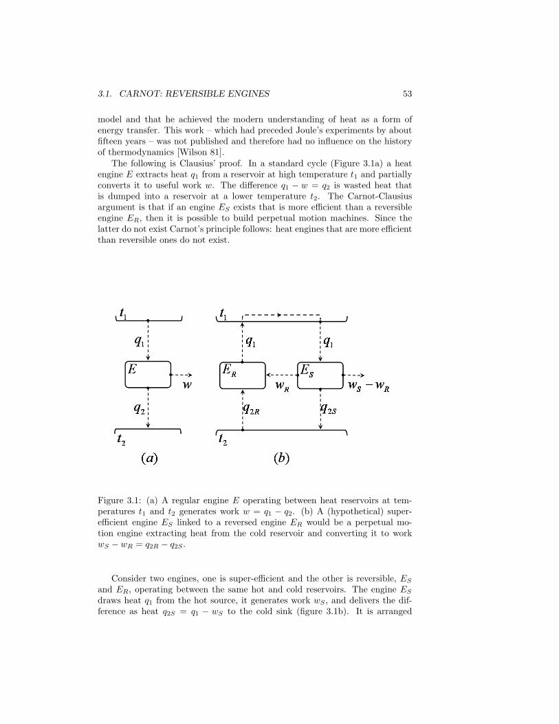
3.1. CARNOT: REVERSIBLE ENGINES 53

model and that he achieved the modern understanding of heat as a form ofenergy transfer. This work – which had preceded Joule’s experiments by aboutfifteen years – was not published and therefore had no influence on the historyof thermodynamics [Wilson 81].

The following is Clausius’ proof. In a standard cycle (Figure 3.1a) a heatengine E extracts heat q1 from a reservoir at high temperature t1 and partiallyconverts it to useful work w. The difference q1 − w = q2 is wasted heat thatis dumped into a reservoir at a lower temperature t2. The Carnot-Clausiusargument is that if an engine ES exists that is more efficient than a reversibleengine ER, then it is possible to build perpetual motion machines. Since thelatter do not exist Carnot’s principle follows: heat engines that are more efficientthan reversible ones do not exist.

Figure 3.1: (a) A regular engine E operating between heat reservoirs at tem-peratures t1 and t2 generates work w = q1 − q2. (b) A (hypothetical) super-efficient engine ES linked to a reversed engine ER would be a perpetual mo-tion engine extracting heat from the cold reservoir and converting it to workwS − wR = q2R − q2S .

Consider two engines, one is super-efficient and the other is reversible, ESand ER, operating between the same hot and cold reservoirs. The engine ESdraws heat q1 from the hot source, it generates work wS , and delivers the dif-ference as heat q2S = q1 − wS to the cold sink (figure 3.1b). It is arranged


that in its normal (forward) operation the reversible engine ER draws the sameheat q1 from the hot source, it generates work wR, and discards the differenceq2R = q1 − wR to the cold sink. Since ES is supposed to be more efficient thanER we have wS > wR, it would be possible to use a part wR of the work pro-duced by ES to run ER in reverse. The result would be to extract heat q2R fromthe cold source and pump the total heat q2R + wR = q1 back up into the hotsource. The remaining work wS −wR produced by ES would then be availablefor any other purposes. At the end of such composite cycle the hot reservoir isleft unchanged and the net result would be to extract heat q2R − q2 > 0 fromthe cold reservoir and convert it to work wS − wR without any need for fuel.The conclusion is that the existence of a super-efficient heat engine would allowthe construction of a perpetual motion engine.

The blank statement perpetual motion is not possible is a true principle butit does not tell the whole story. It blurs the important distinction betweenperpetual motion engines that operate by violating energy conservation, whichare called machines of the first kind, and perpetual motion engines that do notviolate energy conservation, which are thus called machines of the second kind.Carnot’s conclusion deserves to be singled out as a new principle because it isspecific to the second kind of machine.

Other important conclusions obtained by Carnot are that all reversible en-gines operating between the same temperatures are equally efficient; their effi-ciency is a function of the temperatures only,

edef=

w

q1= e(t1, t2) , (3.1)

and is therefore independent of any and all other details of how the engine isconstructed and operated; that efficiency increases with the temperature differ-ence [see eq.(3.3) below]. Furthermore, the most efficient heat engine cycle, nowcalled the Carnot cycle, is one in which all heat is absorbed at the high t1 andall heat is discharged at the low t2. Thus, the Carnot cycle is defined by twoisotherms and two adiabats.

The next important step, the determination of the universal function e(t1, t2),was accomplished by Kelvin.

3.2 Kelvin: temperature

After Joule’s experiments in the 1840’s on the conversion of work into heat thecaloric model had to be abandoned. Heat was finally recognized as a form ofenergy and the additional relation w = q1 − q2 was the ingredient that, in thehands of Kelvin and Clausius, allowed Carnot’s principle to be developed intothe next stage.

Suppose two reversible engines Ea and Eb are linked in series to form a singlemore complex reversible engine Ec. The first operates between temperatures t1and t2, and the second between t2 and t3. Ea draws heat q1 and discharges q2,while Eb uses q2 as input and discharges q3. The efficiencies of the three engines

3.2. KELVIN: TEMPERATURE 55

areea = e (t1, t2) =

waq1

, eb = e (t2, t3) =wbq2

, (3.2)

andec = e (t1, t3) =

wa + wbq1

. (3.3)

They are related by

ec = ea +wbq2

q2

q1= ea + eb

(1− wa

q1

), (3.4)

orec = ea + eb − eaeb , (3.5)

which is a functional equation for e = e (t1, t2). To find the solution changevariables to x = log (1− e), which transforms eq.(3.5) into

xc (t1, t3) = xa (t1, t2) + xb (t2, t3) , (3.6)

and then differentiate with respect to t2 to get

∂

∂t2xa (t1, t2) = − ∂

∂t2xb (t2, t3) . (3.7)

The left hand side is independent of t3 while the second is independent of t1,therefore ∂xa/∂t2 must be some function g of t2 only,

∂

∂t2xa (t1, t2) = g(t2) . (3.8)

Integrating gives x(t1, t2) = F (t1) + G(t2) where the two functions F and Gare at this point unknown. The boundary condition e (t, t) = 0 or equivalentlyx(t, t) = 0 implies that we deal with merely one unknown function: G(t) =−F (t). Therefore

x(t1, t2) = F (t1)− F (t2) or e (t1, t2) = 1− f(t2)f(t1)

, (3.9)

where f = e−F . From eq.(3.3) we see that the efficiency e (t1, t2) increases asthe difference in temperature increases, so that f (t) must be a monotonicallyincreasing function.

Kelvin recognized that there is nothing fundamental about the original tem-perature scale t. It depends on the particular materials employed to constructthe thermometer. Kelvin realized that the freedom in eq.(3.9) in the choice ofthe function f corresponds to the freedom of changing temperature scales byusing different thermometric materials. The only feature common to all ther-mometers that claim to rank systems according to their ‘degree of hotness’ isthat they must agree that if A is hotter than B, and B is hotter than C, thenA is hotter than C. One can therefore regraduate any old inconvenient t scale


by a monotonic function to obtain a new scale T chosen purely because it leadsto a more elegant formulation of the theory. From eq.(3.9) the optimal choiceis quite obvious, and thus Kelvin introduced the absolute scale of temperature,

T = Cf (t) , (3.10)

where the arbitrary scale factor C reflects the still remaining freedom to choosethe units. In the absolute scale the efficiency for the ideal reversible heat engineis very simple,

e (t1, t2) = 1− T2

T1. (3.11)

Carnot’s principle that any heat engine E′ must be less efficient than thereversible one, e′ ≤ e, is rewritten as

e′ =w

q1= 1− q2

q1≤ e = 1− T2

T1, (3.12)

or,q1

T1− q2

T2≤ 0 . (3.13)

It is convenient to redefine heat so that inputs are positive, Q1 = q1, and outputsare negative, Q2 = −q2. Then,

Q1

T1+Q2

T2≤ 0 , (3.14)

where the equality holds when and only when the engine is reversible.The generalization to an engine or any system that undergoes a cyclic process

in which heat is exchanged with more than two reservoirs is straightforward. Ifheat Qi is absorbed from the reservoir at temperature Ti we obtain the Kelvinform (1854) of Carnot’s principle,

∑i

QiTi≤ 0 . (3.15)

which, in the hands of Clausius, led to the next non-trivial step, the introductionof the concept of entropy.

3.3 Clausius: entropy

By about 1850 both Kelvin and Clausius had realized that two laws were nec-essary as a foundation for thermodynamics. The somewhat awkward expres-sions for the second law that they had adopted at the time were reminiscent ofCarnot’s; they stated the impossibility of heat engines whose sole effect wouldbe to transform heat from a single source into work, or of refrigerators that couldpump heat from a cold to a hot reservoir without the input of external work. Ittook Clausius until 1865 – this is some fifteen years later, which indicates that

3.3. CLAUSIUS: ENTROPY 57

the breakthrough was not at all trivial – before he came up with a new compactstatement of the second law that allowed substantial further progress. [Cropper86]

Clausius rewrote Kelvin’s eq.(3.15) for a cycle where the system absorbs in-finitesimal (positive or negative) amounts of heat dQ from a continuous sequenceof reservoirs, ∮ dQ

T≤ 0 , (3.16)

where T is the temperature of each reservoir. For a reversible process, whichis achieved when the system is slowly taken through a sequence of equilibriumstates and T is the temperature of the system as well as the reservoirs, theequality sign implies that the integral from any state A to any other state B isindependent of the path taken,∮ dQ

T= 0⇒

∫R1(A,B)

dQ

T=

∫R2(A,B)

dQ

T, (3.17)

where R1(A,B) and R2(A,B) denote any two reversible paths linking the sameinitial state A and final state B. Clausius saw that this implied the existence ofa function of the thermodynamic state, which he called the entropy, and definedup to an additive constant by

SB = SA +∫

R(A,B)

dQ

T. (3.18)

At this stage in the development this entropy is ‘thermodynamic entropy’, andis defined only for equilibrium states.

Eq.(3.18) seems like a mere reformulation of eqs.( 3.15) and (3.16) but itrepresents a major advance because it allowed thermodynamics to reach beyondthe study of cyclic processes. Consider a possibly irreversible process in whicha system is taken from an initial state A to a final state B, and suppose thesystem is returned to the initial state along some other reversible path. Then,the more general eq.(3.16) gives

B∫A,irrev

dQ

T+

∫R(A,B)

dQ

T≤ 0 . (3.19)

From eq.(3.18) the second integral is SA − SB . In the first integral −dQ is theamount is the amount of heat absorbed by the reservoirs at temperature T andtherefore it represents minus the change in the entropy of the reservoirs, whichin this case represent the rest of the universe,

(SresA − Sres

B ) + (SA − SB) ≤ 0 or SresB + SB ≥ Sres

A + SA . (3.20)

Thus the second law can be stated in terms of the total entropy Stotal = Sres +Sas

Stotalfinal ≥ Stotal

initial , (3.21)


and Clausius could then summarize the laws of thermodynamics as “The energyof the universe is constant. The entropy of the universe tends to a maximum.”All restrictions to cyclic processes have disappeared.

Clausius was also responsible for initiating another independent line of re-search in this subject. His paper “On the kind of motion we call heat” (1857)was the first (failed!) attempt to deduce the second law from purely mechanicalprinciples applied to molecules. His results referred to averages taken over allmolecules, for example the kinetic energy per molecule, and involved theoremsin mechanics such as the virial theorem. For him the increase of entropy wasmeant to be an absolute law and not just a matter of overwhelming probability.

3.4 Maxwell: probability

We owe to Maxwell the introduction of probabilistic notions into fundamentalphysics (1860). (Perhaps he was inspired by his earlier study of the rings ofSaturn which required reasoning about particles undergoing very complex tra-jectories.) He realized the impossibility of keeping track of the exact motion ofall the molecules in a gas and pursued a less detailed description in terms of thedistribution of velocities. Maxwell interpreted his distribution function as thefraction of molecules with velocities in a certain range, and also as the “proba-bility” P (~v)d3v that a molecule has a velocity ~v in a certain range d3v. It wouldtake a long time to achieve a clearer understanding of the meaning of the term‘probability’. In any case, Maxwell concluded that “velocities are distributedamong the particles according to the same law as the errors are distributed inthe theory of the ‘method of least squares’,” and on the basis of this distributionhe obtained a number of significant results on the transport properties of gases.

Over the years he proposed several derivations of his velocity distributionfunction. The earlier one (1860) is very elegant. It involves two assumptions:the first is a symmetry requirement, the distribution should only depend on theactual magnitude |~v| = v of the velocity and not on its direction,

P (v)d3v = P(√

v2x + v2

y + v2z

)d3v . (3.22)

The second assumption is that velocities along orthogonal directions should beindependent

P (v)d3v = p(vx)p(vy)p(vz)d3v . (3.23)

ThereforeP(√

v2x + v2

y + v2z

)= p(vx)p(vy)p(vz) . (3.24)

Setting vy = vz = 0 we get

P (vx) = p(vx)p(0)p(0) , (3.25)

so that we obtain a functional equation for p,

p(√

v2x + v2

y + v2z

)p(0)p(0) = p(vx)p(vy)p(vz) , (3.26)

3.4. MAXWELL: PROBABILITY 59

or

log

p(√

v2x + v2

y + v2z

)p(0)

= log[p(vx)p(0)

]+ log

[p(vy)p(0)

]+ log

[p(vz)p(0)

], (3.27)

or, introducing the functions G,

G(√

v2x + v2

y + v2z

)= G(vx) +G(vy) +G(vz). (3.28)

The solution is straightforward. Differentiate with respect to vx and to vy toget

G′(√

v2x + v2

y + v2z

)√v2x + v2

y + v2z

vx = G′(vx) andG′(√

v2x + v2

y + v2z

)√v2x + v2

y + v2z

vx = G′(vx) ,

(3.29)or

G′(vx)vx

=G′(vy)vy

= −2α , (3.30)

where −2α is a constant. Integrating gives

log[p(vx)p(0)

]= G(vx) = −αv2

x + const , (3.31)

so that

P (v) =(απ

)3/2

exp[−α

(v2x + v2

y + v2z

)], (3.32)

the same distribution as “errors in the method of least squares”.Maxwell’s distribution applies whether the molecule is part of a gas, a liquid,

or a solid and, with the benefit of hindsight, the reason is quite easy to see.The probability that a molecule have velocity ~v and position ~x is given bythe Boltzmann distribution ∝ exp−H/kT . For a large variety of situationsthe Hamiltonian for one molecule is of the form H = mv2/2 + V (~x) wherethe potential V (~x) includes the interactions, whether they be weak or strong,with all the other molecules. If the potential V (~x) is independent of ~v, thenthe distribution for ~v and ~x factorizes. Velocity and position are statisticallyindependent, and the velocity distribution is Maxwell’s.

Maxwell was the first to realize that the second law is not an absolute law(this was expressed in his popular textbook ‘Theory of Heat’ in 1871), that it‘has only statistical certainty’ and indeed, that in fluctuation phenomena ‘thesecond law is continually being violated’. Such phenomena are not rare: justlook out the window and you can see the sky is blue – a consequence of thescattering of light by density fluctuations in the atmosphere.

Maxwell introduced the notion of probability, but what did he actually meanby the word ‘probability’? He used his distribution function as a velocity dis-tribution, the number of molecules with velocities in a certain range, which


betrays a frequentist interpretation. These probabilities are ultimately mechan-ical properties of the gas. But he also used his distribution to represent thelack of information we have about the precise microstate of the gas. This lat-ter interpretation is particularly evident in a letter he wrote in 1867 where heargues that the second law could be violated by “a finite being who knows thepaths and velocities of all molecules by simple inspection but can do no workexcept open or close a hole.” Such a “demon” could allow fast molecules to passthrough a hole from a vessel containing hot gas into a vessel containing coldgas, and could allow slow molecules pass in the opposite direction. The neteffect being the transfer of heat from a low to a high temperature, a violationof the second law. All that was required was that the demon “know” the rightinformation. [Klein 70]

3.5 Gibbs: beyond heat

Gibbs generalized the second law in two directions: to open systems and toinhomogeneous systems. With the introduction of the concept of the chemicalpotential, a quantity that regulates the transfer of particles in much the sameway that temperature regulates the transfer of heat, he could apply the meth-ods of thermodynamics to phase transitions, mixtures and solutions, chemicalreactions, and much else. His paper “On the Equilibrium of Heterogeneous Sys-tems” [Gibbs 1875-78] is formulated as the purest form of thermodynamics –a phenomenological theory of extremely wide applicability because its founda-tions do not rest on particular models about the structure and dynamics of themicroscopic constituents.

And yet, Gibbs was keenly aware of the significance of the underlying molec-ular constitution – he was familiar with Maxwell’s writings and in particularwith his “Theory of Heat” (indeed, he found mistakes in it). His discussion ofthe process of mixing gases led him to analyze the “paradox” that bears hisname. The entropy of two different gases increases when the gases are mixed;but does the entropy also increase when two gases of the same molecular speciesare mixed? Is this an irreversible process?

For Gibbs there never was a ‘paradox’, much less one that would requiresome esoteric new (quantum) physics for its resolution. For him it was quiteclear that thermodynamics was not concerned with microscopic details, butrather with the changes from one macrostate to another. He explained that themixing of two gases of the same molecular species cannot be reversed becausethe mixing does not lead to a different “thermodynamic” state:

“...we do not mean a state in which each particle shall occupy more or lessexactly the same position as at some previous epoch, but only a state whichshall be indistinguishable from the previous one in its sensible properties.It is to states of systems thus incompletely defined that the problems ofthermodynamics relate.” [Gibbs 1875-78]

3.6. BOLTZMANN: ENTROPY AND PROBABILITY 61

Gibbs’ resolution of the paradox hinges on recognizing, as had Maxwell be-fore him, that the explanation of the second law cannot rest on purely me-chanical arguments, that probabilistic concepts are required. This led him toconclude: “In other words, the impossibility of an uncompensated decreaseof entropy seems to be reduced to improbability,” a sentence that Boltzmannadopted as the motto for the second volume of his “Lectures on the Theory ofGases.” (For a modern discussion of the Gibbs’ paradox see section 4.12.)

Remarkably neither Maxwell nor Gibbs established a connection betweenprobability and entropy. Gibbs was very successful at showing what one canaccomplish by maximizing entropy but he did not address the issue of whatentropy is or what it means. The crucial steps in this direction were taken byBoltzmann.

But Gibbs’ contributions did not end here. The ensemble theory introducedin his “Principles of Statistical Mechanics” in 1902 (it was Gibbs who coined theterm ‘statistical mechanics’) represent a practical and conceptual step beyondBoltzmann’s understanding of entropy.

3.6 Boltzmann: entropy and probability

It was Boltzmann who found the connection between entropy and probability,but his path was long and tortuous [Klein 73, Uffink 04]. Over the years headopted several different interpretations of probability and, to add to the con-fusion, he was not always explicit about which one he was using, sometimesmixing them within the same paper, and even within the same equation. Atfirst, he defined the probability of a molecule having a velocity ~v within a smallcell d3v as being proportional to the amount of time that the particle spentwithin that particular cell, but he also defined that same probability as thefraction of particles within the cell.

By 1868 he had managed to generalize the Maxwell distribution for pointparticles and the theorem of equipartition of energy to complex molecules in thepresence of an external field. The basic argument, which led him to the Boltz-mann distribution, was that in equilibrium the distribution should be stationary,that it should not change as a result of collisions among particles.

The collision argument only gave the distribution for individual molecules;it was also in 1868 that he first applied probability to the system as a wholerather than to the individual molecules. He identified the probability of thesystem being in some region of the N -particle phase space (rather than thespace of molecular velocities) with the relative time the system would spendin that region – the so-called “time” ensemble. Alternatively, probability wasalso defined at a given instant in time as being proportional to the volume ofthe region. At first he did not think it was necessary to comment on whetherthe two definitions are equivalent or not, but eventually he realized that their‘probable’ equivalence should be explicitly expressed as the hypothesis, whichlater came to be known as the ‘ergodic hypothesis’, that over a long time thetrajectory of the system would cover the whole region of phase space consistent


with the given value of the energy. At the time all these probabilities were stillconceived as mechanical properties of the gas.

In 1871 Boltzmann achieved a significant success in establishing a connectionbetween thermodynamic entropy and microscopic concepts such as the proba-bility distribution in phase space. In modern notation his argument was asfollows. The energy of N interacting particles is given by

H =N∑i

p2i

2m+ U (x1, . . . , xN ) . (3.33)

The first non-trivial decision was to specify what quantity defined in purelymicroscopic terms corresponds to the macroscopic internal energy. He opted forthe “average”

E = 〈H〉 =∫dzN PN H , (3.34)

where dzN = d3Nxd3Np is the volume element in the N -particle phase space,and PN is the N -particle distribution function,

PN =exp (−βH)

Zwhere Z =

∫dzN e−βH , (3.35)

and β = 1/kT , so that,

E =32NkT + 〈U〉 . (3.36)

The connection to the thermodynamic entropy requires a clear idea of thenature of heat and how it differs from work. One needs to express heat in purelymicroscopic terms, and this is quite subtle because at the molecular level there isno distinction between thermal motions and just plain motions. The distributionfunction is the crucial ingredient. In any infinitesimal transformation the changein the internal energy separates into two contributions,

δE =∫dzN HδPN +

∫dzN PNδH . (3.37)

The second integral, which can be written as 〈δH〉 = 〈δU〉, arises purely fromchanges in the potential function U , which depends among other things onthe volume of the vessel containing the gas. Now, a change in the potentialis precisely what one means by mechanical work δW , therefore, since δE =δQ+ δW , the first integral must represent the transferred heat δQ,

δQ = δE − 〈δU〉 . (3.38)

On the other hand, substituting δE from eq.(3.36), one gets

δQ =32NkδT + δ 〈U〉 − 〈δU〉 . (3.39)

This is not a complete differential, but dividing by the temperature yields

δQ

T= δ

[32Nk log T +

〈U〉T

+ k log(∫d3Nx e−βU

)+ const

], (3.40)

3.6. BOLTZMANN: ENTROPY AND PROBABILITY 63

which suggests that the expression in brackets should be identified with thethermodynamic entropy S. Further rewriting leads to

S =E

T+ k logZ + const , (3.41)

which is recognized as the correct modern expression.Boltzmann’s path towards understanding the second law was guided by one

notion from which he never wavered: matter is an aggregate of molecules. Apartfrom this the story of his progress is the story of the increasingly more impor-tant role played by probabilistic notions, and ultimately, it is the story of theevolution of his understanding of the notion of probability itself. By 1877 Boltz-mann achieves his final goal and explains entropy purely in terms of probability– mechanical notions were by now reduced to the bare minimum consistent withthe subject matter: we are, after all, talking about collections of molecules andtheir energy is conserved. His final achievement hinges on the introduction ofyet another way of thinking about probabilities.

He considered an idealized system consisting of N particles whose single-particle phase space is divided into m cells each with energy εn, n = 1, ...,m.The number of particles in the nth cell is denoted wn, and the distribution‘function’ is given by the set of numbers w1, . . . , wm. In Boltzmann’s previouswork the determination of the distribution function had been based on figur-ing out its time evolution from the mechanics of collisions. Here he used apurely combinatorial argument. A completely specified state, which he called acomplexion, and we call a microstate, is defined by specifying the cell of eachindividual molecule. A macrostate is less completely specified by the distribu-tion function, w1, . . . , wm. The number of microstates compatible with a givenmacrostate, which he called the ‘permutability’, and we call the ‘multiplicity’ is

W =N !

w1! . . . wm!. (3.42)

Boltzmann’s assumption was that the probability of the macrostate was propor-tional to its multiplicity, to the number of ways in which it could be achieved,which assumes each microstate is as likely as any other – the ‘equal a prioriprobability postulate’.

The most probable macrostate is that which maximizes W subject to theconstraints of a fixed total number of particles N and a fixed total energy E,

m∑n=1

wn = N andm∑n=1

wnεn = E. (3.43)

When the numbers wn are large enough that one can use Stirling’s approxima-tion for the factorials, we have

logW = N logN −N −m∑n=1

(wn logwn − wn) (3.44)

= −m∑n=1

wn logwn + const , (3.45)


or perhaps better

logW = −Nm∑n=1

wnN

logwnN

(3.46)

so that

logW = −Nm∑n=1

fn log fn (3.47)

where fn = wn/N is the fraction of molecules in the nth cell with energy εn, or,alternatively the probability that a molecule is in its nth state. The distributionthat maximizes logW subject to the constraints (3.43) is such that

fn =wnN∝ e−βεn , (3.48)

where β is a Lagrange multiplier determined by the total energy. When appliedto a gas, the possible states of a molecule are cells in phase space. Therefore

logW = −N∫dz1 f(x, p) log f(x, p) , (3.49)

where dz1 = d3xd3p and the most probable distribution is the equilibrium dis-tribution found earlier by Maxwell and generalized by Boltzmann.

In this approach probabilities are central. The role of dynamics is minimizedbut it is not eliminated. The Hamiltonian enters the discussion in two places.One is quite explicit: there is a conserved energy the value of which is imposed asa constraint. The second is much more subtle; we saw above that the probabilityof a macrostate could be taken proportional to the multiplicity W providedmicrostates are assigned equal probabilities, or equivalently, equal volumes inphase space are assigned equal a priori weights. As always equal probabilitiesmust be justified in terms of some form of underlying symmetry. In this case, thesymmetry follows from Liouville’s theorem – under a Hamiltonian time evolutiona region in phase space will move around and its shape will be distorted butits volume will be conserved; Hamiltonian time evolution preserves volumes inphase space. The nearly universal applicability of the ‘equal a priori postulate’can be traced to the fact that what is needed is a Hamiltonian; any Hamiltonianwould do.

It is very remarkable that although Boltzmann calculated the maximizedvalue logW for an ideal gas and knew that it agreed with the thermodynamicalentropy except for a scale factor, he never wrote the famous equation that bearshis name

S = k logW . (3.50)

This equation, as well as Boltzmann’s constant k, were both first written byPlanck.

There is, however, a problem with eq.(3.49): it involves the distributionfunction f(x, p) in the one-particle phase space and therefore it cannot takecorrelations into account. Indeed, eq.(3.49) gives the correct form of the entropy

3.7. SOME REMARKS 65

only for ideal gases of non-interacting particles. The expression that applies tosystems of interacting particles is3

logW = −∫dzN fN log fN , (3.51)

where fN = fN (x1, p1, . . . , xN , pN ) is the probability distribution in the N -particle phase space. This equation is usually associated with the name of Gibbswho, in his “Principles of Statistical Mechanics” (1902), developed Boltzmann’scombinatorial arguments into a very powerful theory of ensembles. The con-ceptual gap between eq.(3.49) and (3.51) is enormous; it goes well beyond theissue of intermolecular interactions. The probability in Eq.(3.49) is the single-particle distribution, it can be interpreted as a “mechanical” property, namely,the relative number of molecules in each cell. The entropy Eq.(3.49) is a me-chanical property of the individual system. In contrast, eq.(3.51) involves theN -particle distribution which is not a property of any single individual systembut a property of an ensemble of replicas of the system. Gibbs was not veryexplicit about his interpretation of probability. He wrote

“The states of the bodies which we handle are certainly not known to usexactly. What we know about a body can generally be described mostaccurately and most simply by saying that it is one taken at random froma great number (ensemble) of bodies which are completely described.” [myitalics, Gibbs 1902, p.163]

It is clear that for Gibbs probabilities represent a state of knowledge, that theensemble is a purely imaginary construction, just a tool for handling incompleteinformation. On the other hand, it is also clear that Gibbs still thinks of prob-abilities in terms of frequencies, and since the actual replicas of the system donot exist, he is forced to imagine them.

This brings our story of entropy up to about 1900. In the next chapter westart a more deliberate and systematic study of the connection between entropyand information.

3.7 Some remarks

I end with a disclaimer: this chapter has historical overtones but it is not history.Lines of research such as the Boltzmann equation and the ergodic hypothesisthat were historically very important have been omitted because they representpaths that diverge from the central theme of this work, namely how laws ofphysics can be derived from rules for handling information and uncertainty. Ourgoal has been and will be to discuss thermodynamics and statistical mechanicsas the first historical example of such an information physics. At first I tried towrite a ‘history as it should have happened’. I wanted to trace the development

3For the moment we disregard the question of the distinguishability of the molecules. Theso-called Gibbs paradox and the extra factor of 1/N ! will be discussed in detail in chapter 4.


of the concept of entropy from its origins with Carnot in a manner that reflectsthe logical rather than the actual evolution. But I found that this approachwould not do; it trivializes the enormous achievements of the 19th centurythinkers and it misrepresents the actual nature of research. Scientific researchis not a tidy business.

I mentioned that this chapter was inspired by a beautiful article by E. T.Jaynes with the same title [Jaynes 88]. I think Jaynes’ article has great peda-gogical value but I disagree with him on how well Gibbs understood the logicalstatus of thermodynamics and statistical mechanics as examples of inferentialand probabilistic thinking. My own assessment runs in quite the opposite di-rection: the reason why the conceptual foundations of thermodynamics andstatistical mechanics have been so controversial throughout the 20th century isprecisely because neither Gibbs nor Boltzmann were particularly clear on theinterpretation of probability. I think that we could hardly expect them to havedone much better; they did not benefit from the writings of Keynes (1921),Ramsey (1931), de Finetti (1937), Jeffreys (1939), Cox (1946), Shannon (1948),Polya (1954) and, of course, Jaynes himself (1957). Indeed, whatever clarityJaynes attributes to Gibbs, is not Gibbs’; it is the hard-won clarity that Jaynesattained through his own efforts and after absorbing much of the best the 20thcentury had to offer.

Chapter 4

Entropy II: MeasuringInformation

What is information? Our central goal is to gain insight into the nature ofinformation, how one manipulates it, and the implications of such insights forphysics. In chapter 2 we provided a first partial answer. We might not yet knowprecisely what information is, but we know it when we see it. For example, itis clear that experimental data contains information, that it is processed usingBayes’ rule, and that this is very relevant to the empirical aspect of science,namely, to data analysis. Bayes’ rule is the machinery that processes the in-formation contained in data to update from a prior to a posterior probabilitydistribution. This suggests the following generalization: “information” is what-ever induces one to update from one state of belief to another. This is a notionworth exploring and to which we will return later.

In this chapter we pursue another point of view that has turned out to beextremely fruitful. We saw that the natural way to deal with uncertainty, thatis, with lack of information, is to introduce the notion of degrees of belief, andthat these measures of plausibility should be manipulated and calculated usingthe ordinary rules of the calculus of probabilities. But with this achievementwe do not yet reach our final goal. The rules of probability theory allow us toassign probabilities to some “complex” propositions on the basis of the proba-bilities that have been previously assigned to other, perhaps more “elementary”propositions.

In this chapter we introduce a new inference tool designed specifically forassigning those elementary probabilities. The new tool is Shannon’s measure ofan “amount of information” and the associated method of reasoning is Jaynes’Method of Maximum Entropy, or MaxEnt. [Shannon 48, Jaynes 57b, 83, 03]

67

68 CHAPTER 4. ENTROPY II: MEASURING INFORMATION

4.1 Shannon’s information measure

We appeal once more to the idea that if a general theory exists it must apply tospecial cases. Consider a set of mutually exclusive and exhaustive alternativesi, for example, the possible values of a variable, or the possible states of asystem. The state of the system is unknown. On the basis of the incompleteinformation I we have we can at best assign probabilities p(i|I) = pi. In orderto select just one among the possible states more information is required. Thequestion we address here is how much more? Note that we are not asking themore difficult question of which particular piece of information is missing, butmerely the quantity that is missing. It seems reasonable that the amount ofinformation that is missing in a sharply peaked distribution is smaller than theamount missing in a broad distribution, but how much smaller? Is it possible toquantify the notion of amount of information? Can one find a unique quantityS that is a function of the pi’s, that tends to be large for broad distributionsand small for narrow ones?

Consider a discrete set of n mutually exclusive and exhaustive discrete al-ternatives i, each with probability pi. According to Shannon, any measure Sof the amount of information that is missing when all we know is a probabilitydistribution must satisfy three axioms. It is quite remarkable that these con-ditions are sufficiently constraining to determine the quantity S uniquely. Thefirst two axioms are deceptively simple.Axiom 1. S is a real continuous function of the probabilities pi, S[p] =S (p1, . . . pn).Remark: It is explicitly assumed that S[p] depends only on the pi and onnothing else. What we seek here is an absolute measure of the amount ofmissing information in p. If the objective were to update from a prior q to aposterior distribution p – a problem that will be later tackled in chapter 6 –then we would require a functional S[p, q] depending on both q and p. SuchS[p, q] would at best be a relative measure: the information in p relative to thereference distribution q.Axiom 2. If all the pi’s are equal, pi = 1/n. Then S = S (1/n, . . . , 1/n) =F (n), where F (n) is an increasing function of n.Remark: This means that it takes less information to pinpoint one alternativeamong a few than among many and also that knowing the number n of availablestates is already a valuable piece of information. Notice that the uniform distri-bution pi = 1/n is singled out to play a very special role. Indeed, although noreference distribution has been explicitly mentioned, the uniform distributionwill, in effect, provide the standard of complete ignorance.

The third axiom is a consistency requirement and is somewhat less intuitive.The entropy S[p] measures the amount of additional information beyond the in-complete information I already codified in the pi that will be needed to pinpointthe actual state of the system. Imagine that this missing information were tobe obtained not all at once, but in installments. The consistency requirementis that the particular manner in which we obtain this information should notmatter. This idea can be expressed as follows.

4.1. SHANNON’S INFORMATION MEASURE 69

Imagine the n states are divided into N groups labeled by g = 1, . . . , N . Theprobability that the system is found in group g is

Pg =∑i∈g

pi . (4.1)

Let pi|g denote the conditional probability that the system is in the state i ∈ ggiven it is in group g,

pi|g =piPg

for i ∈ g. (4.2)

Suppose we were to obtain the desired information in two steps, the first ofwhich would allow us to single out one of the groups g while the second wouldallow us to decide on the actual i within the selected group g. The amountof information required in the first step is SG = S[P ] where P = Pg withg = 1 . . . N . Now suppose we did get this information, and as a result we found,for example, that the system was in group g1. Then for the second step, tosingle out the state i within the group g1, the amount of additional informationneeded would be Sg1 = S[p·|g1 ]. Similarly, information amounts Sg2 , Sg3 , . . . orSgN would be required had the selected groups turned out to be g2, g3, . . . or gN .But at the beginning of this process we do not yet know which of the g’s is thecorrect one. The expected amount of missing information to take us from theg’s to the actual i’s is

∑g PgSg. The point is that it should not matter whether

we get the total missing information in one step, which completely determines i,or in two steps, the first of which has low resolution and only determines one ofthe groups, say g, while the second step provides the fine tuning that determinesi within the given g. This gives us our third axiom:Axiom 3. For all possible groupings g = 1 . . . N of the states i = 1 . . . n wemust have

S = SG +∑gPgSg . (4.3)

This is called the “grouping” property.Remark: Given axiom 3 it might seem more appropriate to interpret S as ameasure of the expected rather than the actual amount of missing information,but if S is the expected value of something, it is not clear, at this point, whatthat something would be. We will return to this below.

The solution to Shannon’s constraints is obtained in two steps. First assumethat all states i are equally likely, pi = 1/n. Also assume that the N groups gall have the same number of states, m = n/N , so that Pg = 1/N and pi|g =pi/Pg = 1/m. Then by axiom 2,

S[pi] = S (1/n, . . . , 1/n) = F (n) , (4.4)

SG[Pg] = S (1/N, . . . , 1/N) = F (N) , (4.5)

andSg[pi|g] = S(1/m, . . . , 1/m) = F (m). (4.6)


Then, axiom 3 givesF (mN) = F (N) + F (m) . (4.7)

This should be true for all integers N and m. It is easy to see that one solutionof this equation is

F (m) = k log m , (4.8)

where k is any positive constant, but it is easy to see that eq.(4.7) has infinitelymany other solutions. Indeed, since any integer m can be uniquely decomposedas a product of prime numbers, m =

∏rqαrr , where αi are integers and qr are

prime numbers, using eq.(4.7) we have

F (m) =∑rαrF (qr) (4.9)

which means that eq.(4.7) can be satisfied by arbitrarily specifying F (qr) on theprimes and then defining F (m) for any other integer through eq.(4.9).

A unique solution is obtained when we impose the additional requirementthat F (m) be monotonic increasing in m (axiom 2). The following argument isfound in [Jaynes 03]. Consider any two integers s and t both larger than 1. Theratio of their logarithms can be approximated arbitrarily closely by a rationalnumber, i.e., we can find integers α and β (with β arbitrarily large) such that

α

β≤ log s

log t<α+ 1β

or tα ≤ rβ < tα+1 . (4.10)

But F is monotonic increasing, therefore

F (tα) ≤ F (sβ) < F (tα+1) , (4.11)

and using eq.(4.7),

αF (t) ≤ βF (s) < (α+ 1)F (t) orα

β≤ F (s)F (t)

<α+ 1β

. (4.12)

Which means that the ratio F (r)/F (s) can be approximated by the same ratio-nal number α/β. Indeed, comparing eqs.(4.10) and (4.12) we get∣∣∣∣F (s)

F (t)− log s

log t

∣∣∣∣ ≤ 1β

(4.13)

or, ∣∣∣∣F (s)log s

− F (t)log t

∣∣∣∣ ≤ F (t)β log s

(4.14)

We can make the right hand side arbitrarily small by choosing β sufficientlylarge, therefore F (s)/ log s must be a constant, which proves (4.8) is the uniquesolution.

In the second step of our derivation we will still assume that all is are equallylikely, so that pi = 1/n and S[p] = F (n). But now we assume the groups g havedifferent sizes, mg, with Pg = mg/n and pi|g = 1/mg. Then axiom 3 becomes

F (n) = SG[P ] +∑g

Pg F (mg),

4.1. SHANNON’S INFORMATION MEASURE 71

Therefore,

SG[P ] = F (n)−∑g

PgF (mg) =∑g

Pg [F (n)− F (mg)] .

Substituting our previous expression for F we get

SG[P ] =∑g

Pg k logn

mg= −k

N∑i=1

Pg logPg .

Therefore Shannon’s quantitative measure of the amount of missing information,the entropy of the probability distribution p1, . . . , pn is

S[p] = −kn∑i=1

pi log pi . (4.15)

Comments

Notice that for discrete probability distributions we have pi ≤ 1 and log pi ≤ 0.Therefore S ≥ 0 for k > 0. As long as we interpret S as the amount ofuncertainty or of missing information it cannot be negative. We can also checkthat in cases where there is no uncertainty we get S = 0: if any state hasprobability one, all the other states have probability zero and every term in Svanishes.

The fact that entropy depends on the available information implies thatthere is no such thing as the entropy of a system. The same system may havemany different entropies. Notice, for example, that already in the third axiomwe find an explicit reference to two entropies S[p] and SG[P ] referring to twodifferent descriptions of the same system. Colloquially, however, one does referto the entropy of a system; in such cases the relevant information available aboutthe system should be obvious from the context. In the case of thermodynamicswhat one means by the entropy is the particular entropy that one obtains whenthe only information available is specified by the known values of those fewvariables that specify the thermodynamic macrostate.

The choice of the constant k is purely a matter of convention. A convenientchoice is k = 1. In thermodynamics the choice is Boltzmann’s constant kB =1.38 × 10−16erg/K which reflects the historical choice of units of temperature.In communication theory and computer science, the conventional choice is k =1/ loge 2 ≈ 1.4427, so that

S[p] = −n∑i=1

pi log2 pi . (4.16)

The base of the logarithm is 2, and the entropy is said to measure informationin units called ‘bits’.

Now we turn to the question of interpretation. Earlier we mentioned thatfrom axiom 3 it seems more appropriate to interpret S as a measure of the


expected rather than the actual amount of missing information. If one adoptsthis interpretation, the actual amount of information that we gain when we findthat i is the true alternative would have to be log 1/pi. But this is not quitesatisfactory. Consider a variable that takes just two values, 0 with probability pand 1 with probability 1−p. For very small p, log 1/p would be very large, whilethe information that communicates the true alternative is conveyed by a veryshort one bit message, namely “0”. It appears that it is not the actual amountof information that log 1/p seems to measure but rather how unexpected or howsurprising the piece of information might be. Accordingly, log 1/pi is sometimescalled the “surprise” of i.

It seems reasonable to expect that more information implies less uncertainty.We have used the word ‘uncertainty’ as roughly synonymous to ‘lack of infor-mation’. The following example illustrates the potential pitfalls. I normallykeep my keys in my pocket. My state of knowledge about the location of mykeys is represented by a probability distribution that is sharply peaked at mypocket and reflects a small uncertainty. But suppose I check and I find thatmy pocket is empty. Then my keys could be virtually anywhere. My new stateof knowledge is represented by a very broad distribution that reflects a highuncertainty. We have here a situation where more information has increasedthe uncertainty rather than decreased it.

The point of these remarks is not to suggest that there is something wrongwith the mathematical derivation – eq.(4.15) does follow from the axioms – butto suggest caution when interpreting S. The notion of information is at thispoint still vague. Any attempt to find its measure will always be open to theobjection that it is not clear what it is that is being measured. Indeed, the firsttwo of Shannon’s axioms seem to be particularly intuitive, but the third one,the grouping property, is not nearly as compelling. Is entropy the only way tomeasure uncertainty? Doesn’t the variance also measure uncertainty? Shannonand Jaynes both argued that one should not place too much significance on theaxiomatic derivation of eq.(4.15), that its use can be fully justified a posterioriby its formal properties, for example, by the various inequalities it satisfies.However, this position can be questioned on the grounds that it is the axiomsthat confer meaning to the entropy; the disagreement is not about the actualequations, but about what they mean and, ultimately, about how they shouldbe used. Other measures of uncertainty can be introduced and, indeed, theyhave been introduced by Renyi and by Tsallis, creating a whole industry ofalternative theories. [Renyi 61, Tsallis 88] Whenever one can make an inferenceusing Shannon’s entropy, one can make other inferences using any one of theRenyi’s entropies. Which, among all those alternatives, should one choose?

The two-state case

To gain intuition about S[p] consider the case of a variable that can take twovalues. The proverbial example is a biased coin – for example, a bent coin – forwhich the outcome ‘heads’ is assigned probability p and ‘tails’ probability 1−p.

4.2. RELATIVE ENTROPY 73

The corresponding entropy is

S(p) = −p log p− (1− p) log (1− p) , (4.17)

where we chose k = 1. It is easy to check that S ≥ 0 and that the maximumuncertainty, attained for p = 1/2, is Smax = log 2.

An important set of properties of the entropy follows from the concavityof the entropy which follows from the concavity of the logarithm. Supposewe can’t decide whether the actual probability of heads is p1 or p2. We maydecide to assign probability q to the first alternative and probability 1 − q tothe second. The actual probability of heads then is the mixture qp1 + (1− q)p2.The corresponding entropies satisfy the inequality

S (qp1 + (1− q)p2) ≥ qS (p1) + (1− q)S (p2) , (4.18)

with equality in the extreme cases where p1 = p2, or q = 0, or q = 1. Eq.(4.18)says that however ignorant we might be when we invoke a probability distribu-tion, an uncertainty about the probabilities themselves will introduce an evenhigher degree of ignorance.

4.2 Relative entropy

The following entropy-like quantity turns out to be useful

K[p, q] = +∑i

pi logpiqi. (4.19)

Despite the positive sign K is sometimes read as the ‘entropy of p relative toq,’ and thus called “relative entropy.” It is easy to see that in the special casewhen qi is a uniform distribution then K is essentially equivalent to the Shannonentropy – they differ by a constant. Indeed, for qi = 1/n, eq.(4.19) becomes

K[p, 1/n] =n∑i

pi (log pi + log n) = log n− S[p] . (4.20)

The relative entropy is also known by many other names including crossentropy, information divergence, information for discrimination, and Kullback-Leibler distance [Kullback 59] who recognized its importance for applications instatistics, and studied many of its properties). However, the expression (4.19)has a much older history. It was already used by Gibbs in his ElementaryPrinciples of Statistical Mechanics [Gibbs 1902].

It is common to interpret K[p, q] as the amount of information that is gained(thus the positive sign) when one thought the distribution that applies to arandom process is q and one learns that the distribution is actually p. Theinterpretation suffers from the same conceptual difficulties mentioned earlierconcerning the Shannon entropy. In the next chapter we will see that the relativeentropy turns out to be the fundamental quantity for inference – indeed, more


fundamental, more general, and therefore, more useful than entropy itself – andthat the interpretational difficulties that afflict the Shannon entropy can beavoided. (We will also redefine it with a negative sign, S[p, q] def= −K[p, q], sothat it really is a true entropy.) In this chapter we just derive some propertiesand consider some applications.

An important property of the relative entropy is the Gibbs inequality,

K[p, q] ≥ 0 , (4.21)

with equality if and only if pi = qi for all i. The proof uses the concavity of thelogarithm,

log x ≤ x− 1 or logqipi≤ qipi− 1 , (4.22)

which implies ∑i

pi logqipi≤∑i

(qi − pi) = 0 . (4.23)

The Gibbs inequality provides some justification to the common interpreta-tion of K[p, q] as a measure of the “distance” between the distributions p andq. Although useful, this language is not quite correct because K[p, q] 6= K[q, p]while a true distance d is required to be symmetric, d[p, q] = d[q, p]. However,as we shall later see, if the two distributions are sufficiently close the relativeentropy K[p + δp, p] satisfies all the requirements of a metric. Indeed, it turnsout that up to a constant factor, it is the only natural Riemannian metric onthe manifold of probability distributions. It is known as the Fisher-Rao metricor, perhaps more appropriately, the information metric.

The two inequalities S[p] ≥ 0 and K[p, q] ≥ 0 together with eq.(4.20) imply

0 ≤ S[p] ≤ log n , (4.24)

which establishes the range of the entropy between the two extremes of completecertainty (pi = δij for some value j) and complete uncertainty (the uniformdistribution) for a variable that takes n discrete values.

4.3 Joint entropy, additivity, and subadditivity

The entropy S[px] reflects the uncertainty or lack of information about thevariable x when our knowledge about it is codified in the probability distributionpx. It is convenient to refer to S[px] directly as the “entropy of the variable x”and write

Sxdef= S[px] = −

∑xpx log px . (4.25)

The virtue of this notation is its compactness but one must keep in mind thesame symbol x is used to denote both a variable x and its values xi. To be moreexplicit,

−∑xpx log px = −

∑i

px(xi) log px(xi) . (4.26)

4.4. CONDITIONAL ENTROPY AND MUTUAL INFORMATION 75

The uncertainty or lack of information about two (or more) variables x andy is expressed by the joint distribution pxy and the corresponding joint entropyis

Sxy = −∑xypxy log pxy . (4.27)

When the variables x and y are independent, pxy = pxpy, the joint entropyis additive

Sxy = −∑xypxpy log(pxpy) = Sx + Sy , (4.28)

that is, the joint entropy of independent variables is the sum of the entropiesof each variable. This additivity property also holds for the other measure ofuncertainty we had introduced earlier, namely, the variance,

var(x+ y) = var(x) + var(y) . (4.29)

In thermodynamics additivity is called extensivity : the entropy of an ex-tended system is the sum of the entropies of its parts provided these parts areindependent. The thermodynamic entropy can be extensive only when the in-teractions between various subsystems are sufficiently weak that correlationsbetween them can be neglected.

When the two variables x and y are not independent the equality (4.28)can be generalized into an inequality. Consider the joint distribution pxy =pxpy|x = pypx|y. The relative entropy or Kullback “distance” of pxy to theproduct distribution pxpy that would represent uncorrelated variables is givenby

K[pxy, pxpy] =∑xypxy log

pxypxpy

= −Sxy −∑xypxy log px −

∑xypxy log py

= −Sxy + Sx + Sy . (4.30)

Therefore, using K ≥ 0 we get

Sxy ≤ Sx + Sy , (4.31)

with the equality holding when the two variables x and y are independent.This inequality is called the subadditivity property. Its interpretation is clear:entropy increases when information about correlations is discarded.

4.4 Conditional entropy and mutual information

Consider again two variables x and y. We want to measure the amount ofuncertainty about one variable x when we have some limited information aboutanother variable y. This quantity, called the conditional entropy, and denoted


Sx|y, is obtained by calculating the entropy of x as if the precise value of y wereknown and then taking the expectation over the possible values of y

Sx|y =∑ypyS[px|y] = −

∑ypy∑xpx|y log px|y = −

∑x,ypxy log px|y , (4.32)

where pxy is the joint distribution of x and y.The conditional entropy is related to the entropy of x and the joint entropy

by the following “chain rule.” Use the product rule for the joint distribution

log pxy = log py + log px|y , (4.33)

and take the expectation over x and y to get

Sxy = Sy + Sx|y . (4.34)

In words: the entropy of two variables is the entropy of one plus the conditionalentropy of the other. Also, since Sy is positive we see that conditioning reducesentropy,

Sxy ≥ Sx|y . (4.35)

Another useful entropy-like quantity is the so-called “mutual information”of x and y, denoted Mxy, which “measures” how much information x and y havein common. This is given by the relative entropy between the joint distributionpxy and the product distribution pxpy that discards all information containedin the correlations. Using eq.(4.30),

Mxydef= K[pxy, pxpy] = Sx + Sy − Sxy ≥ 0 , (4.36)

which shows that it is symmetrical in x and y. Using eq.(4.34) the mutualinformation is related to the conditional entropies by

Mxy = Sx − Sx|y = Sy − Sy|x . (4.37)

The relationships among these various entropies can be visualized by a figurethat resembles a Venn diagram. (The diagram is usually considered a purelymnemonic aid, but recent work [Knuth 02-06] on the duality between asser-tions and questions, and the corresponding duality between probabilities andentropies suggests that the resemblance between the two types of Venn diagramsis not accidental.)

4.5 Continuous distributions

Shannon’s derivation of the expression for entropy, eq.(4.15), applies to probabil-ity distributions of discrete variables. The generalization to continuous variablesis not quite straightforward.

The discussion will be carried out for a one-dimensional continuous variable;the generalization to more dimensions is trivial. The starting point is to notethat the expression

−∫dx p(x) log p(x) (4.38)

4.5. CONTINUOUS DISTRIBUTIONS 77

is unsatisfactory. A change of variables x → y = y(x) changes the probabil-ity density p(x) to p′(y) but does not represent a loss or gain of information.Therefore, the actual probabilities do not change, p(x)dx = p′(y)dy, and neithershould the entropy. However, one can check that (4.38) is not invariant,∫

dx p(x) log p(x) =∫dy p′(y) log

[p′(y)

∣∣∣∣dydx∣∣∣∣]

6=∫dy p′(y) log p′(y) . (4.39)

We approach the continuous case as a limit from the discrete case. Considera continuous distribution p(x) defined on an interval for xa ≤ x ≤ xb. Dividethe interval into equal intervals ∆x = (xb − xa) /N . The distribution p(x) canbe approximated by a discrete distribution

pn = p(xn)∆x , (4.40)

where xn = xa + n∆x and n is an integer. The discrete entropy is

SN = −N∑n=0

∆x p(xn) log [p(xn)∆x] , (4.41)

and as N →∞ we get

SN −→ logN −xb∫xa

dx p(x) log[

p(x)1/ (xb − xa)

](4.42)

which diverges. This is quite to be expected: it takes a finite amount of informa-tion to identify one discrete alternative within a finite set, but it takes an infiniteamount to single out one point in a continuum. The difference SN − logN hasa well defined limit and we are tempted to consider

−xb∫xa

dx p(x) log[

p(x)1/ (xb − xa)

](4.43)

as a candidate for the continuous entropy, until we realize that, except foran additive constant, it coincides with the unacceptable expression (4.38) andshould be discarded for precisely the same reason: it is not invariant underchanges of variables. Had we first changed variables to y = y(x) and thendiscretized into N equal ∆y intervals we would have obtained a different limit

−yb∫ya

dy p′(y) log[

p′(y)1/ (yb − ya)

]. (4.44)

The problem is that the limiting procedure depends on the particular choice ofdiscretization; the limit depends on which particular set of intervals ∆x or ∆ywe have arbitrarily decided to call equal. Another way to express the same ideais to note that the denominator 1/ (xb − xa) in (4.43) represents a probabilitydensity that is uniform in the variable x, but not in y. Similarly, the density1/ (yb − ya) in (4.44) is uniform in y, but not in x.


Having identified the origin of the problem we can now suggest a solution.On the basis of our prior knowledge of the problem at hand we must decide ona privileged set of equal intervals, or alternatively, on one preferred probabilitydistribution µ(x) we are willing to define as “uniform.” Then, and only then, itmakes sense to propose the following definition

S[p, µ] def= −xb∫xa

dx p(x) logp(x)µ(x)

. (4.45)

It is easy to check that this is invariant,

xb∫xa

dx p(x) logp(x)µ(x)

=yb∫ya

dy p′(y) logp′(y)µ′(y)

. (4.46)

Examples illustrating possible choices of the uniform µ(x) are the following.

1. When the variable x refers to position in “physical” space, we can feelfairly comfortable with what we mean by equal volumes: use Cartesiancoordinates and choose µ(x) = constant.

2. In a curved space D-dimensional, with a known metric tensor gij , i.e., thedistance between neighboring points with coordinates xi and xi + dxi isgiven by d`2 = gijdx

idxj , the volume elements are given by (det g)1/2dDx.

In this case choose µ(x) ∝ (det g)1/2.

3. In classical statistical mechanics the Hamiltonian evolution in phase spaceis, according to Liouville’s theorem, such that phase space volumes areconserved. This leads to a natural definition of equal intervals or equalvolumes. The corresponding choice of uniform µ is called the postulate of“equal a priori probabilities.”

Notice that the expression in eq.(4.45) is a relative entropy −K[p, µ]. Thisis a hint for a theme that will be fully developed in chapter 6: relative entropyis the more fundamental quantity. Strictly, there is no Shannon entropy in thecontinuum – not only do we have to subtract an infinite constant and spoilits (already shaky) interpretation as an information measure, but we have toappeal to prior knowledge and introduce the measure µ. On the other handthere are no difficulties in obtaining the continuum relative entropy from itsdiscrete version. We can check that

KN =N∑n=0

pn logpnqn

=N∑n=0

∆x p(xn) logp(xn)∆xq(xn)∆x

(4.47)

has a well defined limit,

K[p, q] =xb∫xa

dx p(x) logp(x)q(x)

, (4.48)

which is explicitly invariant under coordinate transformations.

4.6. COMMUNICATION THEORY 79

4.6 Communication Theory

Here we give the briefest introduction to some basic notions of communicationtheory as originally developed by Shannon [Shannon 48, Shannon Weaver 49].For a more comprehensive treatment see [Cover Thomas 91].

Communication theory studies the problem of how a message that was se-lected at some point of origin can be best reproduced at some later destinationpoint. The complete communication system includes an information source thatgenerates a message composed of, say, words in English, or pixels on a picture.A transmitter translates the message into an appropriate signal. For example,sound pressure is encoded into an electrical current, or letters into a sequenceof zeros and ones. The signal is such that it can be transmitted over a commu-nication channel, which could be electrical signals propagating in coaxial cablesor radio waves through the atmosphere. Finally, a receiver reconstructs the sig-nal back into a message that can be interpreted by an agent at the destinationpoint.

From the engineering point of view the communication system must be de-signed with only a limited information about the set of possible messages. Inparticular, it is not known which specific messages will be selected for transmis-sion. The typical sort of questions one wishes to address concern the minimalphysical requirements needed to communicate the messages that could poten-tially be generated by a particular information source. One wants to characterizethe sources, measure the capacity of the communication channels, and learn howto control the degrading effects of noise. And after all this, it is somewhat ironicbut nevertheless true that “information theory” is completely unconcerned withwhether any “information” is being communicated at all. As far as the engi-neering goes, whether the messages convey some meaning or not is completelyirrelevant.

To illustrate the basic ideas consider the problem of “data compression.” Auseful idealized model of an information source is a sequence of random variablesx1, x2, . . . which take values from a finite alphabet of symbols. We will assumethat the variables are independent and identically distributed. (Eliminatingthese limitations is both possible and important.) Suppose that we deal with abinary source in which the variables xi, which are usually called ‘bits’, take thevalues zero or one with probabilities p or 1− p respectively. Shannon’s idea wasto classify the possible sequences x1, . . . , xN into typical and atypical accordingto whether they have high or low probability. For large N the expected numberof zeros and ones is Np and N(1 − p) respectively. The probability of thesetypical sequences is

P (x1, . . . , xN ) ≈ pNp(1− p)N(1−p) , (4.49)

so that

− logP (x1, . . . , xN ) ≈ −N [p log p− (1− p) log(1− p)] = NS(p) (4.50)

where S(p) is the two-state entropy, eq.(4.17), the maximum value of which is


Smax = log 2. Therefore, the probability of typical sequences is roughly

P (x1, . . . , xN ) ≈ e−NS(p) . (4.51)

Since the total probability is less than one, we see that the number of typicalsequences has to be less than about eNS(p) which for large N is considerablyless than the total number of possible sequences, 2N = eN log 2. This fact isvery significant. Transmitting an arbitrary sequence irrespective of whether itis typical or not requires a long message of N bits, but we do not have to wasteresources in order to transmit all sequences. We only need to worry about thefar fewer typical sequences because the atypical sequences are too rare. Thenumber of typical sequences is about

eNS(p) = 2NS(p)/ log 2 = 2NS(p)/Smax (4.52)

and therefore we only need about NS(p)/Smax bits to identify each one ofthem. Thus, it must be possible to compress the original long message intoa much shorter one. The compression might imply some small probability oferror because the actual message might conceivably turn out to be atypical butone can, if desired, avoid any such errors by using one additional bit to flagthe sequence that follows as typical and short or as atypical and long. Actualschemes for implementing the data compression are discussed in [Cover Thomas91].

Next we state these intuitive notions in a mathematically precise way.Theorem: The Asymptotic Equipartition Property (AEP). If x1, . . . , xN areindependent variables with the same probability distribution p(x), then

− 1N

logP (x1, . . . , xN ) −→ S[p] in probability. (4.53)

Proof: If the variables xi are independent, so are their logarithms, log p(xi),

− 1N

logP (x1, . . . , xN ) = − 1N

N∑i

log p(xi) , (4.54)

and the law of large numbers (see section 2.8) gives

limN→∞

Prob[∣∣∣∣− 1

NlogP (x1, . . . , xN ) + 〈log p(x)〉

∣∣∣∣ ≤ ε] = 1 , (4.55)

where− 〈log p(x)〉 = S[p] . (4.56)

This concludes the proof.We can elaborate on the AEP idea further. The typical sequences are those

for which eq.(4.51) or (4.53) is satisfied. To be precise let us define the typicalset AN,ε as the set of sequences with probability P (x1, . . . , xN ) such that

e−N [S(p)+ε] ≤ P (x1, . . . , xN ) ≤ e−N [S(p)−ε] . (4.57)

4.6. COMMUNICATION THEORY 81

Theorem of typical sequences:

(1) For N sufficiently large Prob[AN,ε] > 1− ε.

(2) |AN,ε| ≤ eN [S(p)+ε] where |AN,ε| is the number of sequences in AN,ε.

(3) For N sufficiently large |AN,ε| ≥ (1− ε)eN [S(p)−ε].

In words: the typical set has probability near one, typical sequences are nearlyequally probable (thus the ‘equipartition’), and there are about eNS(p) of them.To summarize:

Almost all events are almost equally likely.

Proof: Eq.(4.55) states that for fixed ε, for any given δ there is an Nδ suchthat for all N > Nδ, we have

Prob[∣∣∣∣− 1

NlogP (x1, . . . , xN ) + S[p]

∣∣∣∣ ≤ ε] ≥ 1− δ . (4.58)

Thus, the probability that the sequence (x1, . . . , xN ) is ε-typical tends to one,and therefore so must Prob[AN,ε]. Setting δ = ε yields part (1). To prove (2)write

1 ≥ Prob[AN,ε] =∑

(x1,...,xN )∈AN,εP (x1, . . . , xN )

≥∑

(x1,...,xN )∈AN,εe−N [S(p)+ε] = e−N [S(p)+ε] |AN,ε| . (4.59)

Finally, from part (1),

1− ε < Prob[AN,ε] =∑

(x1,...,xN )∈AN,εP (x1, . . . , xN )

≤∑

(x1,...,xN )∈AN,εe−N [S(p)−ε] = e−N [S(p)−ε] |AN,ε| , (4.60)

which proves (3).We can now quantify the extent to which messages generated by an infor-

mation source of entropy S[p] can be compressed. A scheme that producescompressed sequences that are more than NS(p)/Smax bits is capable of dis-tinguishing among all the typical sequences. The compressed sequences can bereliably decompressed into the original message. Conversely, schemes that yieldcompressed sequences of fewer than NS(p)/Smax bits cannot describe all typi-cal sequences and are not reliable. This result is known as Shannon’s noiselesschannel coding theorem.


4.7 Assigning probabilities: MaxEnt

Probabilities are introduced to deal with lack of information. The notion thatentropy S[p] can be interpreted as a quantitative measure of the amount ofmissing information has one remarkable consequence: it provides us with amethod to assign probabilities. The idea is simple:

Among all possible probability distributions that agree with whatever we knowselect that particular distribution that reflects maximum ignorance about every-thing else. Since ignorance is measured by entropy, the method is mathematicallyimplemented by selecting the distribution that maximizes entropy subject to theconstraints imposed by the available information. This method of reasoning iscalled the method of Maximum Entropy, and is often abbreviated as MaxEnt.

Ultimately, the method of maximum entropy is based on an ethical principleof intellectual honesty that demands that one should not assume informationone does not have. The idea is quite compelling but its justification relies heavilyon interpreting entropy as a measure of missing information and therein lies itsweakness: to what extent are we sure that entropy is the unique measure ofinformation or of uncertainty?

As a simple illustration of the MaxEnt method in action consider a variablex about which absolutely nothing is known except that it can take n discrete val-ues xi with i = 1 . . . n. The distribution that represents the state of maximumignorance is that which maximizes the entropy subject to the single constraintthat the probabilities be normalized,

∑ipi = 1. Introducing a Lagrange multi-

plier α to handle the constraint, the variation pi → pi + δpi gives

0 = δ

(S[p]− α

∑i

pi

)= −

n∑i=1

(log pi + 1 + α) δpi , (4.61)

so that the selected distribution is

pi = e−1−α or pi =1n, (4.62)

where the multiplier α has been determined from the normalization constraint.We can check that the maximum value attained by the entropy,

Smax = −∑i

1n

log1n

= log n , (4.63)

agrees with eq.(4.24).Remark: The distribution of maximum ignorance turns out to be uniform.It coincides with what we would have obtained using Laplace’s Principle ofInsufficient Reason. It is sometimes asserted that the MaxEnt method providesa proof of Laplace’s principle but such a claim is questionable. As we sawearlier, the privileged status of the uniform distribution was imposed throughthe Shannon’s axioms from the very beginning.

4.8. CANONICAL DISTRIBUTIONS 83

4.8 Canonical distributions

The available information constrains the possible probability distributions. Al-though the constraints can take any form whatsoever, in this section we developthe MaxEnt formalism for the special case of constraints that are linear in theprobabilities. The most important applications are to situations of thermo-dynamic equilibrium where the relevant information is given in terms of theexpected values of those few macroscopic variables such as energy, volume, andnumber of particles over which one has some experimental control. (In the nextchapter we revisit this problem more explicitly.)

The goal is to select the distribution of maximum entropy from within thefamily of all distributions for which the expectations of some functions fk(x),k = 1, 2, . . . have known numerical values F k,⟨

fk⟩

=∑i

pifki = F k , (4.64)

where we set fk(xi) = fki to simplify the notation. In addition there is anormalization constraint,

∑pi = 1. Introducing the necessary multipliers, the

entropy maximization is achieved setting

0 = δ

(S[p]− α

∑i

pi − λk⟨fk⟩)

= −∑i

(log pi + 1 + α+ λkf

ki

)δpi , (4.65)

where we adopt the summation convention that repeated upper and lower indicesare summed over. The solution is the so-called ‘canonical’ distribution,

pi = exp−(λ0 + λkfki ) , (4.66)

where we have set 1 + α = λ0. The normalization constraint determines λ0,

eλ0 =∑i

exp(−λkfki ) def= Z (λ1, λ2, . . .) (4.67)

where we have introduced the partition function Z. Substituting eqs.(4.66)and (4.67) into the other constraints, eqs.(4.64), gives a set of equations thatimplicitly determine the remaining multipliers,

− ∂ logZ∂λk

= F k , (4.68)

and substituting into S[p] = −∑pi log pi we obtain the maximized value of the

entropy,Smax =

∑i

pi(λ0 + λkfki ) = λ0 + λkF

k . (4.69)

Equations (4.66-4.68) are a generalized form of the “canonical” distributionsfirst discovered by Maxwell, Boltzmann and Gibbs. Strictly, the calculation


above only shows that the entropy is stationary, δS = 0. To complete theargument we must show that (4.69) is the absolute maximum rather than justa local extremum or a stationary point.

Consider any other distribution qi that satisfies precisely the same con-straints in eqs.(4.64). According to the basic Gibbs inequality for the relativeentropy of q and the canonical p,

K(q, p) =∑i

qi logqipi≥ 0 , (4.70)

orS[q] ≤ −

∑i

qi log pi . (4.71)

Substituting eq.(4.66) gives

S[q] ≤∑i

qi(λ0 + λkfki ) = λ0 + λkF

k . (4.72)

ThereforeS[q] ≤ S[p] = Smax . (4.73)

In words: within the family of all distributions q that satisfy the constraints(4.64) the distribution that achieves the maximum entropy is the canonicaldistribution p given in eq.(4.66).

Having found the maximum entropy distribution we can now develop theMaxEnt formalism along lines that closely parallel the formalism of statisticalmechanics. Each distribution within the family (4.66) can be thought of as apoint in a continuous space – the manifold of canonical distributions. Eachspecific choice of expected values (F 1, F 2, . . .) determines a unique point withinthe space, and therefore the F k play the role of coordinates. To each point(F 1, F 2, . . .) we can associate a number, the value of the maximized entropy.Therefore, Smax is a scalar field which we denote S(F 1, F 2, . . .) = S(F ). Inthermodynamics it is conventional to drop the suffix ‘max’ and to refer to S(F )as the entropy of the system. This language is inappropriate because it canbe misleading. We should constantly remind ourselves that S(F ) is just oneout of many possible entropies. S(F ) is that particular entropy that measuresthe amount of missing information of a subject whose knowledge consists of thenumerical values of the F s and nothing else. The multiplier

λ0 = logZ(λ1, λ2, . . .) = logZ(λ) (4.74)

is sometimes called the “free energy” because it is closely related to the ther-modynamic free energy,

S(F ) = logZ(λ) + λkFk. (4.75)

The quantities S(F ) and logZ(λ) contain the same information; the equationabove shows that they are Legendre transforms of each other. Just as the F sare obtained from logZ(λ) from eq.(4.68), the λs can be obtained from S(F )

∂S(F )∂F k

=∂ logZ(λ)

∂λj

∂λj∂F k

+∂λj∂F k

F j + λk , (4.76)

4.8. CANONICAL DISTRIBUTIONS 85

or, using eq.(4.68),∂S(F )∂F k

= λk , (4.77)

which shows that the multipliers λk are the components of the gradient of theentropy S(F ) on the manifold of canonical distributions.

A useful extension of the formalism is the following. It is common that thefunctions fk are not fixed but depend on one or more parameters v that canbe externally manipulated, fki = fk(xi, v). For example fki could refer to theenergy of the ith state of the system, and the parameter v could be the volumeof the system or an externally applied magnetic field.

Then a general change in the expected value F k induced by changes in bothfk and λk, is expressed as

δF k = δ⟨fk⟩

=∑i

(piδf

ki + fki δpi

), (4.78)

The first term on the right is

⟨δfk⟩

=∑i

pi∂fki∂v

δv =⟨∂fk

∂v

⟩δv . (4.79)

When F k represents the internal energy then⟨δfk⟩

is a small energy trans-fer that can be controlled through an external parameter v. This suggeststhat

⟨δfk⟩

represents a kind of “generalized work,” δW k, and the expectations⟨∂fk/∂v

⟩are analogues of pressure or susceptibility,

δW k def=⟨δfk⟩

=⟨∂fk

∂v

⟩δv . (4.80)

The second term in eq.(4.78),

δQkdef=∑i

fki δpi = δ⟨fk⟩−⟨δfk⟩

(4.81)

is a kind of “generalized heat”, and

δF k = δW k + δQk (4.82)

is a “generalized first law.”The corresponding change in the entropy is obtained from eq.(4.75),

δS = δ logZ(λ) + δ(λkF k)

= − 1Z

∑i

[δλkf

ki + λkδf

ki

]e−λkf

ki + δλkF

k + λkδFk

= λk(δ⟨fk⟩−⟨δfk⟩), (4.83)

which, using eq.(4.81), gives


δS = λkδQk . (4.84)

It is easy to see that this is equivalent to eq.(4.77) where the partial derivativesare derivatives at constant v.

Thus the entropy remains constant in infinitesimal “adiabatic” processes –those with δQk = 0. From the information theory point of view [see eq.(4.81)]this result is a triviality: the amount of information in a distribution cannotchange when the probabilities do not change,

δpi = 0⇒ δQk = 0⇒ δS = 0 . (4.85)

.

4.9 On constraints and relevant information

The method of maximum entropy has been successful in many applications, butthere are cases where it has failed. Are these symptoms of irreparable flaws ormere examples of misuses of the method? MaxEnt is a method for processinginformation: what information are we talking about? The importance of thisissue cannot be overestimated. Here we collect a few remarks; this is a topic towhich we will return repeatedly.

One point that must be made is that questions about how information isprocessed – and this is the problem that MaxEnt is supposed to address –should not be confused with questions about how the information was obtainedin the first place. These are two separate issues.

Here is an example of a common error. Once we accept that certain con-straints might refer to the expected values of certain variables, how do we decidetheir numerical magnitudes? The numerical values of expectations are seldomknown and one might be tempted to replace expected values by sample averagesbecause it is the latter that are directly available from experiment. But the twoare not the same: Sample averages are experimental data. Expected values arenot experimental data.

For very large samples such a replacement can be justified by the law of largenumbers – there is a high probability that sample averages will approximate theexpected values. However, for small samples using one as an approximation forthe other can lead to incorrect inferences. It is important to realize that theseincorrect inferences do not represent an intrinsic flaw of the MaxEnt method;they are merely a warning of how the MaxEnt method should not be used.

There are many other objections that have been raised against the logicbehind the MaxEnt method. We make no attempt to survey them all; manyhave already received adequate answers (see, e.g., [Jaynes 83] and [Jaynes 03],particularly section 11.8). But some objections remain that are quite legitimateand demand our attention. They revolve around the following question: Oncewe accept that constraints will be in the form of the expected values of certainvariables, how do we decide which variables to choose?

4.9. ON CONSTRAINTS AND RELEVANT INFORMATION 87

When using the MaxEnt method to obtain, say, the canonical Boltzmanndistribution (pi ∝ e−βEi) it has been common to adopt the following language:

(A) We seek the probability distribution that codifies the information we ac-tually have (say, the expected energy) and is maximally unbiased (i.e.maximally ignorant or maximum entropy) about all the other informationwe do not possess.

Many authors find this justification unsatisfactory. Indeed, they might argue,for example, that

(B1) The observed spectrum of black body radiation is whatever it is, inde-pendently of the information that happens to be available to us.

We prefer to phrase the objection differently:

(B2) In most realistic situations the expected value of the energy is not aquantity we happen to know; how, then, can we justify using it as aconstraint?

Alternatively, even when the expected values of some quantities happen to beknown, according to (A) what MaxEnt provides is the best possible inferencesgiven the limited information that is available. This is no mean feat, but thereis no guarantee that the resulting inferences will be any good at all. The pre-dictions of statistical mechanics are spectacularly accurate: how can we hopeto achieve equally spectacular predictions in other fields?

(B3) We need some understanding of which are the “correct” quantities theexpectation values of which codify the relevant information for the problemat hand.

Merely that some particular expected value happens to be known is neither anadequate nor a sufficient explanation.

A partial answer to these objections starts with the observation that whetherthe value of the expected energy is known or not, it is nevertheless still true thatmaximizing entropy subject to the energy constraint leads to the indisputablycorrect family of thermal equilibrium distributions (e.g., the black-body spectraldistribution). The justification behind imposing a constraint on the expectedenergy cannot be that this is a quantity that happens to be known – becauseof the brute fact that it is not known – but rather that the expected energyis the quantity that should be known. Even when its actual numerical valueis unknown, we recognize it as the relevant information without which no suc-cessful predictions are possible. (In the next chapter we revisit this importantquestion.)

Therefore we allow MaxEnt to proceed as if this crucial information wereavailable which leads us to a family of distributions containing the temperatureas a free parameter. The actual value of this parameter will have to be inferred


from the experiment itself either directly, using a thermometer, or indirectly byBayesian analysis from other empirical data.

To summarize: It is not just what you happen to know; you have to knowthe right thing. The constraints that should be imposed are those that codifythe information that is relevant to the problem under consideration. Betweenone extreme of ignorance (we know neither which variables are relevant northeir expected values), and the other extreme of useful knowledge (we knowwhich variables are relevant and we also know their expected values), thereis an intermediate state of knowledge – and this is the rule rather than theexception – in which the relevant variables have been correctly identified buttheir actual expected values remain unknown. In this intermediate state, theinformation about which are the relevant variables is taken into account usingMaxEnt to select a parametrized family of probability distributions, while theactual expected values must then be inferred independently either by directmeasurement or inferred indirectly using Bayes’ rule from other experimentaldata.

Achieving this ‘intermediate state of knowledge’ is the difficult problem pre-sented by (B3). Historically progress has been achieved in individual casesmostly by “intuition,” that is, trial and error. Perhaps the seeds for a moresystematic “theory of relevance” can already be seen in the statistical theoriesof model selection and of non-parametric density estimation.

Chapter 5

Statistical Mechanics

Among the various theories that make up what we call physics, thermodynamicsholds a very special place because it provided the first example of a fundamentaltheory that could be interpreted as a procedure for processing relevant infor-mation. Our goal in this chapter is to provide a more explicit discussion ofstatistical mechanics as a theory of inference. We show that several notoriouslycontroversial topics such as the Second Law of thermodynamics, irreversibil-ity, reproducibility, and the Gibbs paradox can be considerably clarified whenviewed from the information/inference perspective.

Since the success of any problem of inference hinges on identifying the rele-vant information we start by providing some background on the dynamical evo-lution of probability distributions – Liouville’s theorem – and then we justifywhy in situations of thermal equilibrium the relevant constraint is encapsulatedinto the expected value of the energy (and/or other such conserved quantities).

5.1 Liouville’s theorem

Perhaps the most relevant, and therefore, most important piece of informationthat has to be incorporated into any inference about physical systems is thattheir time evolution is constrained by equations of motion. Whether these equa-tions – those of Newton, Maxwell, Yang and Mills, or Einstein – can themselvesbe derived as examples of inference are questions which will not concern us atthis point.

To be specific, in this section we will limit ourselves to discussing classicalsystems such as fluids. In this case there is an additional crucial piece of relevantinformation: these systems are composed of molecules. For simplicity we willassume that the molecules have no internal structure, that they are describedby their positions and momenta, and that they behave according to classicalmechanics.

The import of these remarks is that the proper description of the microstateof a fluid of N particles in a volume V is in terms of a “vector” in the N -particle

89

90 CHAPTER 5. STATISTICAL MECHANICS

phase space, z = (~x1, ~p1, . . . ~xN , ~pN ). The time evolution is given by Hamilton’sequations,

d~xidt

=∂H

∂~piand

d~pidt

= −∂H∂~xi

, (5.1)

where H is the Hamiltonian,

H =N∑i=1

p2i

2m+ U(~x1, . . . ~xN , V ) . (5.2)

But the actual positions and momenta of the molecules are unknown and thusthe macrostate of the fluid is described by a probability density in phase space,f(z, t). When the system evolves continuously according to Hamilton’s equa-tions there is no information loss and the probability flow satisfies a local con-servation equation,

∂

∂tf(z, t) = −∇z · J(z, t) , (5.3)

where the probability current J is a vector given by

J(z, t) = f(z, t)z =f(z, t)

d~xidt, f(z, t)

d~pidt

. (5.4)

Evaluating the divergence explicitly using (5.1) gives

∂f

∂t= −

N∑i=1

[∂

∂~xi·(f(z, t)

d~xidt

)+

∂

∂~pi·(f(z, t)

d~pidt

)]= −

N∑i=1

(∂f

∂~xi· ∂H∂~pi− ∂f

∂~pi· ∂H∂~xi

). (5.5)

Thus the time derivative of f(z, t) at a fixed point z is given by the Poissonbracket with the Hamiltonian H,

∂f

∂t= H, f def=

N∑i=1

(∂H

∂~xi· ∂f∂~pi− ∂H

∂~pi· ∂f∂~xi

). (5.6)

This is called the Liouville equation.Two important corollaries are the following. Instead of focusing on the

change in f(z, t) at a fixed point z we can study the change in f (z(t), t) at apoint z(t) that is being carried along by the flow. This defines the so-called“convective” time derivative,

d

dtf (z(t), t) =

∂

∂tf(z, t) +

N∑i=1

(∂f

∂~xi· d~xidt

+∂f

∂~pi· d~pidt

). (5.7)

Using Hamilton’s equations shows that the second term is −H, f and cancelsthe first, therefore

d

dtf (z(t), t) = 0 , (5.8)

5.2. DERIVATION OF EQUAL A PRIORI PROBABILITIES 91

which means that f is constant along a flow line. Explicitly,

f (z(t), t) = f (z(t′), t′) . (5.9)

Next consider a small volume element ∆z(t) that is being carried along bythe fluid flow. Since trajectories cannot cross each other (because Hamilton’sequations are first order in time) they cannot cross the boundary of the evolvingvolume ∆z(t) and therefore the total probability within ∆z(t) is conserved,

d

dtProb[∆z(t)] =

d

dt[∆z(t)f (z(t), t)] = 0 . (5.10)

But f itself is constant, eq.(5.8), therefore

d

dt∆z(t) = 0 , (5.11)

which means that the shape of a region of phase space may get deformed bytime evolution but its volume remains invariant.

5.2 Derivation of Equal a Priori Probabilities

Earlier, in section 4.5, we pointed out that a proper definition of entropy in acontinuum, eq.(4.45), requires that one specify a privileged background measureµ(z),

S[f, µ] = −∫dz f(z) log

f(z)µ(z)

, (5.12)

where dz = d3Nxd3Np. The choice of µ(z) is important: it determines what wemean by a uniform or maximally ignorant distribution.

It is customary to set µ(z) equal to a constant which we might as wellchoose to be one. This amounts to postulating that equal volumes of phasespace are assigned the same a priori probabilities. Ever since the introduction ofBoltzmann’s ergodic hypothesis there have been many failed attempts to deriveit from purely dynamical considerations. In this section we want to determineµ(z) by proving the following theoremThe Equal a Priori Probability Theorem: Since Hamiltonian dynamicsinvolves no loss of information, if the entropy S[f, µ] is to be interpreted as themeasure of amount of information, then µ(z) must be a constant in phase space.Remark: In chapter 6 the requirement that the entropy S must be interpretedas a measure of information will be removed and thus the logic of statisticalmechanics as a theory of inference will be considerably strengthened.Proof: The main non-dynamical hypothesis is that entropy measures informa-tion. The information entropy of the time-evolved distribution f(z, t) is

S(t) = −∫dz f(z, t) log

f(z, t)µ(z)

. (5.13)


The first input from Hamiltonian dynamics is that information is not lost andtherefore we must require that S(t) be constant,

d

dtS(t) = 0 . (5.14)

Therefore,

d

dtS(t) = −

∫dz

[∂f(z, t)∂t

logf(z, t)µ(z)

+∂f(z, t)∂t

]. (5.15)

The second term vanishes,∫dz

∂f(z, t)∂t

=d

dt

∫dz f(z, t) = 0 . (5.16)

A second input from Hamiltonian dynamics is that probabilities are not merelyconserved, they are locally conserved, which is expressed by eqs.(5.3) and (5.4).The first term of eq.(5.15) can be rewritten,

d

dtS(t) =

∫dz∇z · J(z, t) log

f(z, t)µ(z)

, (5.17)

so that integrating by parts (the surface term vanishes) gives

d

dtS(t) = −

∫dz f(z, t)z · ∇z log

f(z, t)µ(z)

=∫dz [−z · ∇zf(z, t) + f(z, t)z · ∇z logµ(z)] . (5.18)

Hamiltonian dynamics enters here once again: the first term vanishes by Liou-ville’s equation (5.6),

−∫dz z · ∇zf(z, t) =

∫dz H, f(z, t) =

∫dz

∂f(z, t)∂t

= 0 , (5.19)

and therefore, imposing (5.14),

d

dtS(t) =

∫dz f(z, t)z · ∇z logµ(z) = 0 . (5.20)

This integral must vanish for any arbitrary choice of the distribution f(z, t),therefore

z · ∇z logµ(z) = 0 . (5.21)

Furthermore, we have considerable freedom about the particular Hamiltonianoperating on the system. We could choose to change the volume in any arbi-trarily prescribed way by pushing on a piston, or we could choose to vary anexternal magnetic field. Either way we can change H(t) and therefore z at will.The time derivative dS/dt must still vanish irrespective of the particular choiceof the vector z. We conclude that

∇z logµ(z) = 0 or µ(z) = const . (5.22)

5.3. THE RELEVANT CONSTRAINTS 93

To summarize: the requirement that information is not lost in Hamiltoniandynamics implies that the measure of information must be a constant of themotion,

d

dtS(t) = 0 , (5.23)

and this singles out the Gibbs entropy,

S(t) = −∫dz f(z, t) log f(z, t) , (5.24)

as the correct information entropy.It is sometimes asserted that (5.23) implies that the Gibbs entropy cannot

be identified with the thermodynamic entropy because this would be in contra-diction to the second law. As we shall see below, this is not true; in fact, it isquite the opposite.

5.3 The relevant constraints

Thermodynamics is concerned with situations of thermal equilibrium. What isthe relevant information needed to make inferences that apply to these specialcases? The first condition we must impose on f (z, t) to describe equilibrium isthat it be independent of time. Thus we require that H, f = 0 and f must be afunction of conserved quantities such as energy, momentum, angular momentum,or number of particles. But we do not want f to be merely stationary, as say,for a rotating fluid, we want it to be truly static. We want f to be invariantunder time reversal. For these problems it turns out that it is not necessary toimpose that the total momentum and total angular momentum vanish; theseconstraints will turn out to be satisfied automatically. To simplify the situationeven more we will only consider problems where the number of particles is heldfixed. Processes where particles are exchanged as in the equilibrium between aliquid and its vapor, or where particles are created and destroyed as in chemicalreactions, constitute an important but straightforward extension of the theory.

It thus appears that it is sufficient to impose that f be some function of theenergy. According to the formalism developed in section 4.8 and the remarks in4.9 this is easily accomplished: the constraints codifying the information thatcould be relevant to problems of thermal equilibrium should be the expectedvalues of functions φ(E) of the energy. For example, 〈φ(E)〉 could includevarious moments, 〈E〉, 〈E2〉,. . . or perhaps more perhaps complicated functions.The remaining question is which functions φ(E) and how many of them.

To answer this question we look at thermal equilibrium from the point of viewleading to what is known as the microcanonical formalism. Let us enlarge ourdescription to include the system of interest A and its environment, that is, thethermal bath B with which it is in equilibrium. The advantage of this broaderview is that the composite system C = A + B can be assumed to be isolatedand we know that its energy Ec is some fixed constant. This is highly relevantinformation: when the value of Ec is known, not only do we know 〈Ec〉 but weknow the expected values 〈φ(Ec)〉 for absolutely all functions φ(Ec). In other


words, in this case we have succeeded in identifying the relevant information andwe are finally ready to assign probabilities using the MaxEnt method. (Whenthe value of Ec is not known we are in that state of “intermediate” knowledgedescribed in section 4.9.)

To simplify the notation it is convenient to divide phase space into discretecells of equal volume. For system A let the (discretized) microstate za haveenergy Ea. For the thermal bath B a much less detailed description is sufficient.Let the number of bath microstates with energy Eb be ΩB(Eb). Our relevantinformation includes the fact that A and B interact very weakly, just barelyenough to attain equilibrium, and thus the known total energy Ec constrainsthe allowed microstates of A+B to the subset that satisfies

Ea + Eb = Ec . (5.25)

The total number of such microstates is

Ω(Ec) =∑aΩB(Ec − Ea) . (5.26)

We are in a situation where we know absolutely nothing beyond the fact thatthe composite system C can be in any one of its Ω(Ec) allowed microstates.This is precisely the problem tackled in section 4.7: the maximum entropydistribution is uniform, eq.(4.62), and the probability of any microstate of C is1/Ω(Ec). More importantly, the probability that system A is in the particularmicrostate a when it is in thermal equilibrium with the bath B is

pa =ΩB(Ec − Ea)

Ω(Ec). (5.27)

This is the result we sought; now we need to interpret it. It is convenient torewrite pa in terms of the the entropy of the bath SB = k log ΩB ,

pa ∝ exp1kSB(Ec − Ea) . (5.28)

There is one final piece of relevant information we can use: the thermal bath Bis much larger than system A, Ec Ea, and we can Taylor expand

SB(Ec − Ea) = SB(Ec)−EaT

+ . . . , (5.29)

where the temperature T of the bath has been introduced according to thestandard thermodynamic definition,

∂SB∂Eb

∣∣∣∣Ec

def=1T. (5.30)

The term SB(Ec) is a constant independent of the label a which can be absorbedinto the normalization. We conclude that the distribution that codifies therelevant information about equilibrium is

pa ∝ exp(−EakT

), (5.31)

5.4. THE CANONICAL FORMALISM 95

which we recognize as having the canonical form of eq.(4.66).Our goal in this section was to identify the relevant variables. Here is the

answer: the relevant information about thermal equilibrium can be summarizedby the expected value of the energy 〈E〉 because someone who just knows 〈E〉and is maximally ignorant about everything else is led to assign probabilitiesaccording to eq.(4.66) which coincides with (5.31).

But our analysis has also disclosed an important limitation. Eq.(5.27) showsthat in general the distribution for a system in equilibrium with a bath dependsin a complicated way on the properties of the bath. The information in 〈E〉is adequate only when the system and the bath interact weakly and the bathis so much larger than the system that its effects can be represented by a sin-gle parameter, the temperature T . Conversely, if these conditions are not met,then more information is needed. For example, the system might be sufficientlyisolated that within the time scales of interest it can only reach thermal equi-librium with the few degrees of freedom in its very immediate vicinity. Thenthe surrounding bath need not be large and the information contained in theexpected value 〈E〉 while still useful and relevant might just not be sufficient;more will be needed.Remark: The notion of relevance is relative. A particular piece of informationmight be relevant to one specific question and irrelevant to another. In thediscussion above the system is in equilibrium, but we have not been sufficientlyexplicit about what specific questions one wants to address. It is implicit in thiswhole approach that one refers to the typical questions addressed in thermody-namics.

5.4 The canonical formalism

We consider a system (say, a fluid) in thermal equilibrium. The energy of the(conveniently discretized) microstate za is Ea = Ea(V ) where V is the volume ofthe system. We assume further that the expected value of the energy is known,〈E〉 = E.

Maximizing the (discretized) Gibbs entropy,

S[p] = −k∑apa log pa where pa = f(za)∆z , (5.32)

subject to constraints on normalization 〈1〉 = 1 and energy 〈E〉 = E yields,eq.(4.66),

pa =1Ze−βEa (5.33)

where the Lagrange multiplier β is determined from

− ∂ logZ∂β

= E and Z(β, V ) =∑ae−βEa . (5.34)

The maximized value of the Gibbs entropy is, eq.(4.69),

S(E, V ) = k logZ + kβE . (5.35)


Differentiating with respect to E we obtain the analogue of eq.(4.77),(∂S

∂E

)V

= k∂ logZ∂β

∂β

∂E+ k

∂β

∂EE + kβ = kβ , (5.36)

where eq.(5.34) has been used to cancel the first two terms. In thermodynamicstemperature is defined by (

∂S

∂E

)V

def=1T, (5.37)

therefore,

β =1kT

. (5.38)

The connection between the formalism above and thermodynamics hinges ona suitable identification of work and heat. A small change in the internal energyδE can be induced by small changes in T and V ,

δE =∑apaδEa +

∑aEaδpa . (5.39)

Since Ea = Ea(V ) the first term 〈δE〉 is an energy change that can be inducedby small changes in volume,

〈δE〉 =∑apa

∂Ea∂V

δV =⟨∂E

∂V

⟩δV , (5.40)

this suggests that we can identify it with the mechanical work,

〈δE〉 = δW = −PδV , (5.41)

and therefore, the pressure is given by

P = −⟨∂E

∂V

⟩. (5.42)

This is the microscopic definition of pressure.The second term in eq.(5.39) must therefore represent heat,

δQ = δE − δW = δ 〈E〉 − 〈δE〉 . (5.43)

The corresponding change in entropy is obtained from eq.(5.35),

δS

k= δ logZ + δ(βE)

= − 1Z

∑ae−βEa (Eaδβ + βδEa) + Eδβ + βδE

= β(δE − 〈δE〉) , (5.44)

therefore,

δS =δQ

T. (5.45)

This result is important. It proves that

5.5. THE SECOND LAW OF THERMODYNAMICS 97

The maximized Gibbs entropy, S(E, V ), is identical to the thermodynamicentropy originally defined by Clausius.

Substituting into eq.(5.43), yields the fundamental thermodynamic identity,

δE = TδS − PδV . (5.46)

Incidentally, it shows that the “natural” variables for energy are S and V , thatis, E = E(S, V ). Similarly, writing

δS =1TδE +

P

TδV (5.47)

confirms that S = S(E, V ).The free energy F is defined by

Z = e−βF or F = −kT logZ(T, V ) . (5.48)

Eq.(5.35) then leads toF = E − TS , (5.49)

so thatδF = −SδT − PδV , (5.50)

which shows that F = F (T, V ).Several useful thermodynamic relations can be easily obtained from eqs.(5.46),

(5.47), and (5.50). For example, the identities(∂F

∂T

)V

= −S and(∂F

∂V

)V

= −P , (5.51)

can be read directly from eq.(5.50).

5.5 The Second Law of Thermodynamics

We saw that in 1865 Clausius summarized the two laws of thermodynamics into“The energy of the universe is constant. The entropy of the universe tends toa maximum.” We can be a bit more explicit about the Second Law: “In anadiabatic non-quasi-static process that starts and ends in equilibrium the totalentropy increases; if the process is adiabatic and quasi-static process the totalentropy remains constant.” The Second Law was formulated in a somewhatstronger form by Gibbs (1878) “For irreversible processes not only does theentropy tend to increase, but it does increase to the maximum value allowed bythe constraints imposed on the system.”

We are now ready to prove the Second Law. The proof below proposed byE. T. Jaynes in 1965 is mathematically very simple, but it is also conceptuallysubtle [Jaynes 65]. It may be useful to recall some of our previous results. The


entropy mentioned in the Second Law is the “thermodynamic” entropy ST . Itis defined only for equilibrium states by the Clausius relation,

ST (B)− ST (A) =B∫A

dQ

T, (5.52)

where the integral is along a reversible path of intermediate equilibrium states.But as we saw in the previous section, in thermal equilibrium the maximizedGibbs entropy Scan

G – that is, the entropy computed from the canonical distri-bution – satisfies the same relation, eq.(5.45),

δScanG =

δQ

T⇒ Scan

G (B)− ScanG (A) =

B∫A

dQ

T. (5.53)

If the arbitrary additive constant is adjusted so ScanG matches ST for one equi-

librium state they will be equal for all equilibrium states. Therefore, if at anytime t the system is in thermal equilibrium and its relevant macrovariables agreewith expected values, say Xt, calculated using the canonical distribution then,

ST (t) = ScanG (t) . (5.54)

The system, which is assumed to be thermally insulated from its environ-ment, is allowed (or forced) to evolve according to a certain Hamiltonian. Theevolution could, for example, be the free expansion of a gas into vacuum, or itcould be given by the time-dependent Hamiltonian that describes some exter-nally prescribed influence, say, a moving piston or an imposed field. Eventuallya new equilibrium is reached at some later time t′. Such a process is adiabatic;no heat was exchanged with the environment. Under these circumstances theinitial canonical distribution fcan(t), e.g. eq.(4.66) or (5.33), evolves accordingto Liouville’s equation, eq.(5.6),

fcan(t)H(t)−→ f(t′) , (5.55)

and, according to eq.(5.23), the corresponding Gibbs entropy remains constant,

ScanG (t) = SG(t′) . (5.56)

Since the Gibbs entropy remains constant it is sometimes argued that thiscontradicts the Second Law but note that the time-evolved SG(t′) is not thethermodynamic entropy because f(t′) is not necessarily of the canonical form,eq.(4.66).

From the new distribution f(t′) we can, however, compute the expectedvalues Xt′ that apply to the state of equilibrium at t′. Of all distributionsagreeing with the new values Xt′ the canonical distribution fcan(t′) is that whichhas maximum Gibbs entropy, Scan

G (t′). Therefore

SG(t′) ≤ ScanG (t′) . (5.57)

5.5. THE SECOND LAW OF THERMODYNAMICS 99

But ScanG (t′) coincides with the thermodynamic entropy of the new equilibrium

state,

ScanG (t′) = ST (t′) . (5.58)

Collecting all these results, eqs.(5.54)-(5.58), we conclude that the thermody-namic entropy has increased,

ST (t) ≤ ST (t′) , (5.59)

which is the Second Law. The equality applies when the time evolution is qua-sistatic so that throughout the process the distribution is always canonical; inparticular, f(t′) = fcan(t′). The argument above can be generalized consider-ably by allowing heat exchanges or by introducing uncertainties into the actualHamiltonian dynamics.

To summarize, the chain of steps is

ST (t) =(1)ScanG (t) =

(2)SG(t′) ≤

(3)ScanG (t′) =

(4)ST (t′) . (5.60)

Steps (1) and (4) hinge on identifying the maximized Gibbs entropy with thethermodynamic entropy – which works provided we have correctly identifiedthe relevant macrovariables for the particular problem at hand. Step (2) followsfrom the constancy of the Gibbs entropy under Hamiltonian evolution – this isthe least controversial step. Of course, if we did not have complete knowledgeabout the exact Hamiltonian H(t) acting on the system an inequality wouldhave been introduced already at this point. The crucial inequality, however, isintroduced in step (3) where information is discarded. The distribution f(t′)contains information about the macrovariables Xt′ at time t′, and since theHamiltonian is known, it also contains information about the values Xt themacrovariables had at the initial time t. In contrast, a description in terms ofthe distribution fcan(t′) contains information about the macrovariables Xt′ attime t′ and nothing else. In a thermodynamic description all memory of thehistory of the system is lost.

The Second Law refers to thermodynamic entropies only. These entropiesmeasure the amount of information available to someone with only macroscopicmeans to observe and manipulate the system. The irreversibility implicit in theSecond Law arises from this restriction to thermodynamic descriptions.

It is important to emphasize what has just been proved: in an adiabaticprocess from one state of equilibrium to another the thermodynamic entropyincreases. This is the Second Law. Many questions remain unanswered: Wehave assumed that the system tends towards and finally reaches an equilibrium;how do we know that this happens? What are the relaxation times, transportcoefficients, etc.? There are all sorts of aspects of non-equilibrium irreversibleprocesses that remain to be explained but this does not detract from whatJaynes’ explanation did in fact accomplish, namely, it explained the SecondLaw, no more and, most emphatically, no less.


5.6 The thermodynamic limit

If the Second Law “has only statistical certainty” (Maxwell, 1871) and anyviolation “seems to be reduced to improbability” (Gibbs, 1878) how can ther-modynamic predictions attain so much certainty? Part of the answer hinges onrestricting the kind of questions we are willing to ask to those concerning the fewmacroscopic variables over which we have some control. Most other questionsare not “interesting” and thus they are never asked. For example, suppose weare given a gas in equilibrium within a cubic box, and the question is where willparticle #23 be found. The answer is that we expect the particle to be at thecenter of the box but with a very large standard deviation – the particle can beanywhere in the box. The answer is not particularly impressive. On the otherhand, if we ask for the energy of the gas at temperature T , or how it changesas the volume is changed by δV , then the answers are truly impressive.

Consider a system in thermal equilibrium in a macrostate described by acanonical distribution f(z) assigned on the basis of constraints on the values ofcertain macrovariables X. For simplicity we will assume X is a single variable,the energy, X = 〈E〉 = E. The microstates z can be divided into typical andatypical microstates. The typical microstates are all contained within a “highprobability” region Rε to be defined below that has total probability 1 − ε,where ε is a small positive number, and within which f(z) is greater than somelower bound. The “phase” volume of the typical region is

Vol(Rε) =∫Rεdz = Wε . (5.61)

Our goal is to establish that the thermodynamic entropy and the volume of theregion Rε are related through Boltzmann’s equation,

ST ≈ k logWε . (5.62)

The surprising feature is that the result is essentially independent of ε. The fol-lowing theorems which are adaptations of the Asymptotic Equipartition Prop-erty (section 4.6) state this result in a mathematically precise way.Theorem: Let f(z) be the canonical distribution and kS = SG = ST thecorresponding entropy,

f(z) =e−βE(z)

Zand S = βE + logZ . (5.63)

Then as N →∞,

− 1N

log f(z) −→ S

Nin probability, (5.64)

provided that the system is such that the energy fluctuations increase slowerthan N , that is, limN→∞∆E/N = 0. (∆ denotes the standard deviation.)

The theorem roughly means that

The accessible microstates are essentially equally likely.

5.6. THE THERMODYNAMIC LIMIT 101

Microstates z for which (− log f(z))/N differs substantially from S/N have ei-ther too low probability and are deemed “inaccessible,” or they might individ-ually have a high probability but are too few to contribute significantly.Remark: The word ‘essentially’ is tricky because f(z) may differ from e−S

by a huge factor, but log f(z) differs from −S by an unimportant amount thatgrows less rapidly than N .Remark: Note that the theorem applies only to those systems with interparti-cle interactions such that the energy fluctuations are sufficiently well behaved.Typically this requires that as N and V tend to infinity with N/V constant, thespatial correlations fall sufficiently fast that distant particles are uncorrelated.Under these circumstances energy and entropy are extensive quantities.Proof: Apply the Tchebyshev inequality (see section 2.8),

P (|x− 〈x〉| ≥ ε) ≤(

∆xε

)2

, (5.65)

to the variablex =

−1N

log f(z) . (5.66)

The mean is the entropy per particle,

〈x〉 =−1N〈log f〉

=S

N=

1N

(βE + logZ

). (5.67)

To calculate the variance,

(∆x)2 =1N2

[⟨(log f)2

⟩− 〈log f〉2

], (5.68)

use ⟨(log f)2

⟩=⟨

(βE + logZ)2⟩

= β2⟨E2⟩

+ 2β 〈E〉 logZ + (logZ)2, (5.69)

so that

(∆x)2 =β2

N2

(⟨E2⟩− 〈E〉2

)=(β∆EN

)2

. (5.70)

Collecting these results gives

Prob[∣∣∣∣− 1

Nlog f(z)− S

N

∣∣∣∣ ≥ ε] ≤ (β∆ENε

)2

. (5.71)

For systems such that the relative energy fluctuations ∆E/E tend to 0 as N−1/2

when N →∞, and the energy is an extensive quantity, E ∝ N , the limit on theright is zero, ∆E/N → 0, therefore,


limN→∞

Prob[∣∣∣∣− 1

Nlog f(z)− S

N

∣∣∣∣ ≥ ε] = 0 , (5.72)

which concludes the proof.The following theorem elaborates on these ideas further. To be precise let

us define the typical region Rε as the set of microstates with probability f(z)such that

e−S−Nε ≤ f(z) ≤ e−S+Nε , (5.73)

or, using eq.(5.63),

1Ze−βE−Nε ≤ f(z) ≤ 1

Ze−βE+Nε . (5.74)

This last expression shows that typical microstates are those for which the en-ergy per particle E(z)/N lies within a narrow interval 2εkT about the expectedvalue E/N .Remark: Even though some states z (namely those with energy E(z) < E) canindividually be more probable than the typical states it turns out (see below)that they are too few and their volume is negligible compared to Wε.Theorem of typical microstates: For N sufficiently large

(1) Prob[Rε] > 1− ε

(2) Vol(Rε) = Wε ≤ eS+Nε.

(3) Wε ≥ (1− ε)eS−Nε.

(4) limN→∞(logWε − S)/N = 0.

In words:

The typical region has probability close to one; typical microstates arealmost equally probable; the phase volume they occupy is about eST /k, thatis, ST = k logW .

The Gibbs entropy is a measure of the logarithm of the phase volume of typicalstates and for large N it does not much matter what we mean by typical (i.e.,what we choose for ε). Incidentally, note that it is the Gibbs entropy thatsatisfies the Boltzmann formula SG = k logW .Proof: Eq.(5.72) states that for fixed ε, for any given δ there is an Nδ suchthat for all N > Nδ, we have

Prob[∣∣∣∣− 1

Nlog f(z)− S

N

∣∣∣∣ ≤ ε] ≥ 1− δ . (5.75)

Thus, the probability that the microstate z is ε-typical tends to one, and there-fore so must Prob[Rε]. Setting δ = ε yields part (1). This also shows that the

5.7. INTERPRETATION OF THE SECOND LAW 103

total probability of the set of states with E(z) < E is negligible – they mustoccupy a negligible volume. To prove (2) write

1 ≥ Prob[Rε] =∫Rεdz f(z)

≥ e−S−Nε∫Rεdz = e−S−NεWε . (5.76)

Similarly, to prove (3) use (1),

1− ε < Prob[Rε] =∫Rεdz f(z)

≤ e−S+Nε∫Rεdz = e−S+NεWε , (5.77)

Finally, from (2) and (3),

(1− ε)eS−Nε ≤Wε ≤ eS+Nε , (5.78)

which is the same as

S

N− ε+

log(1− ε)N

≤ logWε

N≤ S

N+ ε , (5.79)

and proves (4).Remark: The theorems above can be generalized to situations involving severalmacrovariables Xk in addition to the energy. In this case, the expected valueof log f(z) is

〈− log f〉 = S = λk⟨Xk⟩

+ logZ , (5.80)

and its variance is

(∆ log f)2 = λkλm(⟨XkXm

⟩−⟨Xk⟩〈Xm〉

). (5.81)

5.7 Interpretation of the Second Law: Repro-ducibility

We saw that the Gibbs entropy is a measure of the logarithm of the phasevolume of typical states. In the proof of the Second Law (section 4.11.1) westarted with a system at time t in a state of thermal equilibrium defined by themacrovariables Xt. We saw (section 4.11.2) that within the typical region R(t)fluctuations of the Xt are negligible: all microstates are characterized by thesame values of X. Furthermore, the typical region R(t) includes essentially allpossible initial states compatible with the initial Xt.

The volume W (t) = eST (t)/k of the typical region can be interpreted in twoways. On one hand it is a measure of our ignorance as to the true microstatewhen all we know are the macrovariables Xt. On the other hand, the volumeW (t) is also a measure of the extent that we can control the actual microstateof the system when the Xt are the only parameters we can manipulate.

Having been prepared in equilibrium at time t the system is then subjectedto an adiabatic process and it eventually attains a new equilibrium at time t′.


The Hamiltonian evolution deforms the initial region R(t) into a new regionR(t′) with exactly the same volume W (t) = W (t′); the macrovariables evolvefrom their initial values Xt to new values Xt′ .

Now suppose we adopt a thermodynamic description for the new equilibrium;the preparation history is forgotten, and all we know are the new values Xt′ .The new typical regionR′(t′) has a volume W ′(t′) and it includes all microstatescompatible with the information Xt′ .

After these preliminaries we come to the crux of the argument: With thelimited experimental means at our disposal we can guarantee that the initialmicrostate will be somewhere within W (t) and therefore that in due courseof time it will be within W (t′). In order for the process Xt → Xt′ to beexperimentally reproducible it must be that all microstates in W (t′) will alsobe within W ′(t′) which means that W (t) = W (t′) ≤ W ′(t′). Conversely, ifit were true that W (t) > W ′(t′) we would sometimes observe that an initialmicrostate within W (t) would evolve into a final microstate lying outside W ′(t′)that is, sometimes we would observe Xt 9 Xt′ . Thus, when W (t) > W ′(t′) theexperiment is not reproducible.

A new element has been introduced into the discussion of the Second Law:reproducibility. [Jaynes 65] Thus, we can express the Second Law in the some-what tautological form:

In a reproducible adiabatic process the thermodynamic entropy cannot de-crease.

We can address this question from a different angle: How do we know thatthe chosen constraints X are the relevant macrovariables that provide an ade-quate thermodynamic description? In fact, what do we mean by an adequatedescription? Let us rephrase these questions differently: Could there exist addi-tional unknown physical constraints Y that significantly restrict the microstatescompatible with the initial macrostate and which therefore provide an even bet-ter description? The answer is that such variables can, of course, exist butthat including them in the description does not necessarily lead to an improve-ment. If the process Xt → Xt′ is reproducible when no particular care has beentaken to control the values of Y we can expect that to the extent that we areonly interested in the X’s the Y ’s are irrelevant; keeping track of them will notyield a better description. Reproducibility is the criterion whereby we can decidewhether a particular thermodynamic description is adequate or not.

5.8 Remarks on irreversibility

A considerable source of confusion on the question of reversibility is that thesame word ‘reversible’ is used with several different meanings [Uffink 01]:(a) Mechanical or microscopic reversibility refers to the possibility of reversingthe velocities of every particle. Such reversals would allow the system not justto retrace its steps from the final macrostate to the initial macrostate but itwould also allow it to retrace its detailed microstate trajectory as well.

5.9. ENTROPIES, DESCRIPTIONS AND THE GIBBS PARADOX 105

(b) Carnot or macroscopic reversibility refers to the possibility of retracing thehistory ofmacrostates of a system in the opposite direction. The required amount ofcontrol over the system can be achieved by forcing the system along a prescribedpath of intermediate macroscopic equilibrium states that are infinitesimally closeto each other. Such a reversible process is normally and appropriately calledquasi-static. There is no implication that the trajectories of the individualparticles will be retraced.(c) Thermodynamic reversibility refers to the possibility of starting from a finalmacrostate and completely recovering the initial macrostate without any otherexternal changes. There is no need to retrace the intermediate macrostates inreverse order. In fact, rather than ‘reversibility’ it may be more descriptive torefer to ‘recoverability ’. Typically a state is irrecoverable when there is friction,decay, or corruption of some kind.

Notice that when one talks about the “irreversibility” of the Second Law andabout the “reversibility” of mechanics there is no inconsistency or contradiction:the word ‘reversibility’ is being used with two entirely different meanings.

Classical thermodynamics assumes that isolated systems approach and even-tually attain a state of equilibrium. The state of equilibrium is, by definition,a state that, once attained, will not spontaneously change in the future. Onthe other hand, it is understood that changes might have happened in the past.Classical thermodynamics introduces a time asymmetry: it treats the past andthe future differently.

The situation with statistical mechanics is, however, somewhat different.Once equilibrium has been attained fluctuations are possible. In fact, if we waitlong enough we can expect that large fluctuations can be expected to happen inthe future, just as they might have happened in the past. The situation is quitesymmetric. The interesting asymmetry arises when we realize that for a largefluctuation to happen spontaneously in the future might require an extremelylong time while we just happen to know that a similarly large “fluctuation” wasobserved in the very recent past. This might seem strange because the formalismof statistical mechanics does not introduce any time asymmetry. The solutionto the puzzle is that the large “fluctuation” in the recent past most likely didnot happen spontaneously but was quite deliberately brought about by human(or otherwise) intervention. The system was prepared in some unusual state byapplying appropriate constraints which were subsequently removed – we do thisall the time.

5.9 Entropies, descriptions and the Gibbs para-dox

Under the generic title of “Gibbs Paradox” one usually considers a number ofrelated questions in both phenomenological thermodynamics and in statisticalmechanics: (1) The entropy change when two distinct gases are mixed happens


to be independent of the nature of the gases. Is this in conflict with the ideathat in the limit as the two gases become identical the entropy change shouldvanish? (2) Should the thermodynamic entropy of Clausius be an extensivequantity or not? (3) Should two microstates that differ only in the exchange ofidentical particles be counted as two or just one microstate?

The conventional wisdom asserts that the resolution of the paradox restson quantum mechanics but this analysis is unsatisfactory; at best it is incom-plete. While it is true that the exchange of identical quantum particles doesnot lead to a new microstate this approach ignores the case of classical, andeven non-identical particles. For example, nanoparticles in a colloidal suspen-sion or macromolecules in solution are both classical and non-identical. Severalauthors (e.g., [Grad 61, Jaynes 92]) have recognized that quantum theory hasno bearing on the matter; indeed, as remarked in section 3.5, this was alreadyclear to Gibbs.

Our purpose here is to discuss the Gibbs paradox from the point of view ofinformation theory. The discussion follows [Tseng Caticha 01]. Our conclusionwill be that the paradox is resolved once it is realized that there is no such thingas the entropy of a system, that there are many entropies. The choice of entropyis a choice between a description that treats particles as being distinguishableand a description that treats them as indistinguishable; which of these alterna-tives is more convenient depends on the resolution of the particular experimentbeing performed.

The “grouping” property of entropy, eq.(4.3),

S[p] = SG[P ] +∑gPgSg[p·|g]

plays an important role in our discussion. It establishes a relation between twodifferent descriptions and refers to three different entropies. One can describethe system with high resolution as being in a microstate i (with probabilitypi), or alternatively, with lower resolution as being in one of the groups g (withprobability Pg). Since the description in terms of the groups g is less detailedwe might refer to them as ‘mesostates’. A thermodynamic description, on theother hand, corresponds to an even lower resolution that merely specifies theequilibrium macrostate. For simplicity, we will define the macrostate with asingle variable, the energy. Including additional variables is easy and does notmodify the gist of the argument.

The standard connection between the thermodynamic description in terms ofmacrostates and the description in terms of microstates is established in section4.10.4. If the energy of microstate a is Ea, to the macrostate of energy E = 〈E〉we associate that canonical distribution (5.33)

pa =e−βEa

ZH, (5.82)

where the partition function ZH and the Lagrange multiplier β are determinedfrom eqs.(5.34),

ZH =∑i

e−βEi and∂ logZH∂β

= −E . (5.83)


The corresponding entropy, eq.(5.35) is (setting k = 1)

SH = βE + logZH , (5.84)

measures the amount of information required to specify the microstate when allwe know is the value E .

Identical particles

Before we compute and interpret the probability distribution over mesostatesand its corresponding entropy we must be more specific about which mesostateswe are talking about. Consider a system of N classical particles that are exactlyidentical. The interesting question is whether these identical particles are also“distinguishable.” By this we mean the following: we look at two particles nowand we label them. We look at the particles later. Somebody might haveswitched them. Can we tell which particle is which? The answer is: it depends.Whether we can distinguish identical particles or not depends on whether wewere able and willing to follow their trajectories.

A slightly different version of the same question concerns an N -particle sys-tem in a certain state. Some particles are permuted. Does this give us a differentstate? As discussed earlier the answer to this question requires a careful speci-fication of what we mean by a state.

Since by a microstate we mean a point in the N -particle phase space, thena permutation does indeed lead to a new microstate. On the other hand, ourconcern with permutations suggests that it is useful to introduce the notion ofa mesostate defined as the group of those N ! microstates that are obtained aspermutations of each other. With this definition it is clear that a permutationof the identical particles does not lead to a new mesostate.

Now we can return to discussing the connection between the thermodynamicmacrostate description and the description in terms of mesostates using, asbefore, the Method of Maximum Entropy. Since the particles are (sufficiently)identical, all those N ! microstates i within the same mesostate g have the sameenergy, which we will denote by Eg (i.e., Ei = Eg for all i ∈ g). To themacrostate of energy E = 〈E〉 we associate the canonical distribution,

Pg =e−βEg

ZL, (5.85)

whereZL =

∑ge−βEg and

∂ logZL∂β

= −E . (5.86)

The corresponding entropy, eq.(5.35) is (setting k = 1)

SL = βE + logZL , (5.87)

measures the amount of information required to specify the mesostate when allwe know is E.


Two different entropies SH and SL have been assigned to the same macrostateE; they measure the different amounts of additional information required tospecify the state of the system to a high resolution (the microstate) or to a lowresolution (the mesostate).

The relation between ZH and ZL is obtained from

ZH =∑i

e−βEi = N !∑ge−βEg = N !ZL or ZL =

ZHN !

. (5.88)

The relation between SH and SL is obtained from the “grouping” property,eq.(4.3), with S = SH and SG = SL, and pi|g = 1/N !. The result is

SL = SH − logN ! . (5.89)

Incidentally, note that

SH = −∑apa log pa = −

∑gPg logPg/N ! . (5.90)

Equations (5.88) and (5.89) both exhibit the Gibbs N ! “corrections.” Our analy-sis shows (1) that the justification of the N ! factor is not to be found in quantummechanics, and (2) that the N ! does not correct anything. The N ! is not a fudgefactor that fixes a wrong (possibly nonextensive) entropy SH into a correct (pos-sibly extensive) entropy SL. Both entropies SH and SL are correct. They differbecause they measure different things: one measures the information to specifythe microstate, the other measures the information to specify the mesostate.

An important goal of statistical mechanics is to provide a justification, anexplanation of thermodynamics. Thus, we still need to ask which of the twostatistical entropies, SH or SL, should be identified with the thermodynamicentropy of Clausius ST . Inspection of eqs.(5.88) and (5.89) shows that, as longas one is not concerned with experiments that involve changes in the numberof particles, the same thermodynamics will follow whether we set SH = ST orSL = ST .

But, of course, experiments involving changes in N are very important (forexample, in the equilibrium between different phases, or in chemical reactions).Since in the usual thermodynamic experiments we only care that some numberof particles has been exchanged, and we do not care which were the actual par-ticles exchanged, we expect that the correct identification is SL = ST . Indeed,the quantity that regulates the equilibrium under exchanges of particles is thechemical potential defined by

µ = −kT(∂ST∂N

)E,V,...

(5.91)

The two identifications SH = ST or SL = ST , lead to two different chemicalpotentials, related by

µL = µH −NkT . (5.92)

It is easy to verify that, under the usual circumstances where surface effectscan be neglected relative to the bulk, µL has the correct functional dependence


on N : it is intensive and can be identified with the thermodynamic µ. On theother hand, µH is not an intensive quantity and cannot therefore be identifiedwith µ.

Non-identical particles

We saw that classical identical particles can be treated, depending on the res-olution of the experiment, as being distinguishable or indistinguishable. Herewe go further and point out that even non-identical particles can be treated asindistinguishable. Our goal is to state explicitly in precisely what sense it is upto the observer to decide whether particles are distinguishable or not.

We defined a mesostate as a subset of N ! microstates that are obtained aspermutations of each other. With this definition it is clear that a permutationof particles does not lead to a new mesostate even if the exchanged particlesare not identical. This is an important extension because, unlike quantumparticles, classical particles cannot be expected to be exactly identical down toevery minute detail. In fact in many cases the particles can be grossly different –examples might be colloidal suspensions or solutions of organic macromolecules.A high resolution device, for example an electron microscope, would reveal thatno two colloidal particles or two macromolecules are exactly alike. And yet,for the purpose of modelling most of our macroscopic observations it is notnecessary to take account of the myriad ways in which two particles can differ.

Consider a system of N particles. We can perform rather crude macroscopicexperiments the results of which can be summarized with a simple phenomeno-logical thermodynamics where N is one of the relevant variables that define themacrostate. Our goal is to construct a statistical foundation that will explainthis macroscopic model, reduce it, so to speak, to “first principles.” The par-ticles might ultimately be non-identical, but the crude phenomenology is notsensitive to their differences and can be explained by postulating mesostates gand microstates i with energies Ei ≈ Eg, for all i ∈ g, as if the particles wereidentical. As in the previous section this statistical model gives

ZL =ZHN !

with ZH =∑i

e−βEi , (5.93)

and the connection to the thermodynamics is established by postulating

ST = SL = SH − logN ! . (5.94)

Next we consider what happens when more sophisticated experiments areperformed. The examples traditionally offered in discussions of this sort refer tothe new experiments that could be made possible by the discovery of membranesthat are permeable to some of the N particles but not to the others. Other,perhaps historically more realistic examples, are afforded by the availabilityof new experimental data, for example, more precise measurements of a heatcapacity as a function of temperature, or perhaps measurements in a range oftemperatures that had previously been inaccessible.


Suppose the new phenomenology can be modelled by postulating the exis-tence of two kinds of particles. (Experiments that are even more sophisticatedmight allow us to detect three or more kinds, perhaps even a continuum ofdifferent particles.) What we previously thought were N identical particles wewill now think as being Na particles of type a and Nb particles of type b. Thenew description is in terms of macrostates defined by Na and Nb as the relevantvariables.

To construct a statistical explanation of the new phenomenology from ‘firstprinciples’ we need to revise our notion of mesostate. Each new mesostate willbe a group of microstates which will include all those microstates obtained bypermuting the a particles among themselves, and by permuting the b particlesamong themselves, but will not include those microstates obtained by permutinga particles with b particles. The new mesostates, which we will label g and towhich we will assign energy εg, will be composed of Na!Nb! microstates ı, eachwith a well defined energy Eı = Eg, for all ı ∈ g. The new statistical modelgives

ZL =ZH

Na!Nb!with ZH =

∑ı

e−βEı , (5.95)

and the connection to the new phenomenology is established by postulating

ST = SL = SH − logNa!Nb! . (5.96)

In discussions of this topic it is not unusual to find comments to the effectthat in the limit as particles a and b become identical one expects that theentropy of the system with two kinds of particles tends to the entropy of asystem with just one kind of particle. The fact that this expectation is not metis one manifestation of the Gibbs paradox.

From the information theory point of view the paradox does not arise becausethere is no such thing as the entropy of the system, there are several entropies.It is true that as a → b we will have ZH → ZH , and accordingly SH → SH ,but there is no reason to expect a similar relation between SL and SL becausethese two entropies refer to mesostates g and g that remain different even asa and b became identical. In this limit the mesostates g, which are useful fordescriptions that treat particles a and b as indistinguishable among themselvesbut distinguishable from each other, lose their usefulness.

Conclusion

The Gibbs paradox in its various forms arises from the widespread misconceptionthat entropy is a real physical quantity and that one is justified in talking aboutthe entropy of the system. The thermodynamic entropy is not a property of thesystem. Entropy is a property of our description of the system, it is a property ofthe macrostate. More explicitly, it is a function of the macroscopic variables usedto define the macrostate. To different macrostates reflecting different choices ofvariables there correspond different entropies for the very same system.


But this is not the complete story: entropy is not just a function of themacrostate. Entropies reflect a relation between two descriptions of the samesystem: in addition to the macrostate, we must also specify the set of mi-crostates, or the set of mesostates, as the case might be. Then, having specifiedthe macrostate, an entropy can be interpreted as the amount of additional in-formation required to specify the microstate or mesostate. We have found the‘grouping’ property very valuable precisely because it emphasizes the depen-dence of entropy on the choice of micro or mesostates.

Chapter 6

Entropy III: UpdatingProbabilities

The general problem of inductive inference is to update from a prior probabilitydistribution to a posterior distribution when new information becomes available.The challenge is to develop updating methods that are both systematic andobjective. In Chapter 2 we saw that Bayes’ rule is the natural way to updatewhen the information is in the form of data. We also saw that Bayes’ rule couldnot be derived just from the requirements of consistency implicit in the sumand product rules of probability theory. An additional Principle of MinimalUpdating (PMU) was necessary: Prior information is valuable and should notbe discarded; beliefs should be revised only to the extent required by the data. Afew interesting questions were just barely hinted at: How do we update whenthe information is not in the form of data? If the information is not data, whatelse could it possibly be? Indeed what, after all, is information?

Then in Chapter 4 we saw that the method of maximum entropy, MaxEnt,allowed one to deal with information in the form of constraints on the allowedprobability distributions. So here we have a partial answer to one of our ques-tions: in addition to data information can take the form of constraints. However,MaxEnt is not a method for updating; it is a method for assigning probabilitieson the basis of the constraint information, but it does not allow us to take intoaccount the information contained in prior distributions.

Thus, Bayes’ rule allows for the information contained in arbitrary priorsand in data, but not in arbitrary constraints,1 while on the other hand, Max-Ent can handle arbitrary constraints but not arbitrary priors. In this chapterwe bring those two methods together: by generalizing the PMU we show howthe MaxEnt method can be extended beyond its original scope, as a rule toassign probabilities, to a full-fledged method for inductive inference, that is,a method for updating from arbitrary priors given information in the form of

1Bayes’ rule can handle constraints when they are expressed in the form of data that canbe plugged into a likelihood function. Not all constraints are of this kind.

113

114 CHAPTER 6. ENTROPY III: UPDATING PROBABILITIES

arbitrary constraints. It should not be too surprising that the extended Max-imum Entropy method, which we will henceforth abbreviate as ME, includesboth MaxEnt and Bayes’ rule as special cases.

Historically the ME method is a direct descendant of MaxEnt. As we sawin chapter 4 within the MaxEnt method entropy is interpreted through theShannon axioms as a measure of the amount of uncertainty or of the amountof information that is missing in a probability distribution. We discussed somelimitations of this approach. The Shannon axioms refer to probabilities of dis-crete variables; for continuous variables the entropy is not defined. But a moreserious objection was raised: even if we grant that the Shannon axioms do leadto a reasonable expression for the entropy, to what extent do we believe theaxioms themselves? Shannon’s third axiom, the grouping property, is indeedsort of reasonable, but is it necessary? Is entropy the only consistent measureof uncertainty or of information? What is wrong with, say, the standard de-viation? Indeed, there exist examples in which the Shannon entropy does notseem to reflect one’s intuitive notion of information [Uffink 95]. Other entropies,justified by a different choice of axioms, can be introduced (prominent examplesare [Renyi 61, Tsallis 88]).

From our point of view the real limitation is that neither Shannon nor Jayneswere concerned with updating probabilities. Shannon was analyzing the ca-pacity of communication channels and characterizing the potential diversity ofmessages generated by information sources (section 4.6). His entropy makes noreference to prior distributions. On the other hand, as we already mentioned,Jaynes conceived MaxEnt as a method to assign probabilities on the basis ofconstraint information and a fixed underlying measure, not an arbitrary prior.He never meant to update from one probability distribution to another.

Considerations such as these motivated several attempts to develop ME di-rectly as a method for updating probabilities without invoking questionablemeasures of uncertainty. Prominent among them are [Shore and Johnson 80,Skilling 88-90, Csiszar 91]. The important contribution by Shore and Johnsonwas the realization that one could axiomatize the updating method itself ratherthan the information measure. Their axioms are justified on the basis of a fun-damental principle of consistency – if a problem can be solved in more than oneway the results should agree – but the axioms themselves and other assump-tions they make have raised some objections [Karbelkar 86, Uffink 95]). Despitesuch criticism Shore and Johnson’s pioneering papers have had an enormousinfluence; they identified the correct goal to be achieved.

Another approach to entropy was proposed by Skilling. His axioms areclearly inspired by those of Shore and Johnson but his approach is different inseveral important aspects. in particular Skilling did not explore the possibilityof using his induction method for the purpose for inductive inference, that is,for updating from prior to posterior probabilities.

The primary goal of this chapter is to apply Skilling’s method of eliminativeinduction to Shore and Johnson’s problem of updating probabilities and, inthe process, to overcome the objections that can be raised against either. Thepresentation below follows [Caticha 03, Caticha Giffin 06, Caticha 07].

115

As we argued earlier when developing the theory of degrees of belief, ourgeneral approach differs from the way in which many physical theories have beendeveloped in the past. The more traditional approach consists of first settingup the mathematical formalism and then seeking an acceptable interpretation.The drawback of this procedure is that questions can always be raised about theuniqueness of the proposed interpretation, and about the criteria that makes itacceptable or not.

In contrast, here we proceed in the opposite order: we first decide what weare talking about, what goal we want to achieve, and only then we design asuitable mathematical formalism. The advantage is that the issue of meaningand interpretation is resolved from the start. The preeminent example of thisapproach is Cox’s algebra of probable inference (discussed in chapter 2) whichclarified the meaning and use of the notion of probability: after Cox it wasno longer possible to raise doubts about the legitimacy of the degree of beliefinterpretation. A second example is special relativity: the actual physical sig-nificance of the x and t appearing in the mathematical formalism of Lorentz andPoincare was a matter of controversy until Einstein settled the issue by derivingthe formalism,that is, the Lorentz transformations, from more basic principles.Yet a third example is the derivation of the mathematical formalism of quantumtheory. [Caticha 98] In this chapter we explore a fourth example: the concept ofrelative entropy is introduced as a tool for reasoning which reduces to the usualentropy in the special case of uniform priors. There is no need for an interpre-tation in terms of heat, multiplicity of states, disorder, uncertainty, or even interms of an amount of information. In this approach we find an explanationfor why the search for the meaning of entropy has turned out to be so elusive:Entropy needs no interpretation. We do not need to know what ‘entropy’ means;we only need to know how to use it.

Since the PMU is the driving force behind both Bayesian and ME updatingit is worthwhile to investigate the precise relation between the two. We showthat Bayes’ rule can be derived as a special case of the ME method.2 The virtueof our derivation, which hinges on translating information in the form of datainto a constraint that can be processed using ME, is that it is particularly clear.It throws light on Bayes’ rule and demonstrates its complete compatibility withME updating. A slight generalization of the same ideas shows that Jeffrey’supdating rule (section 2.10.2) is also a special case of the ME method. Thus,within the ME framework maximum entropy and Bayesian methods are unifiedinto a single consistent theory of inference.

There is a second function that the ME method must perform in order tofully qualify as a method of inductive inference: once we have decided that thedistribution of maximum entropy is to be preferred over all others the followingquestion arises immediately: the maximum of the entropy function is neverinfinitely sharp, are we really confident that distributions with entropy veryclose to the maximum are totally ruled out? We must find a quantitative way

2This result was first obtained by Williams (see [Williams 80, Diaconis 82]) long before thelogical status of the ME method – and therefore the full extent of its implications – had beensufficiently clarified.


to assess the extent to which distributions with lower entropy are ruled out.This matter is addressed following the treatment in [Caticha 00].

6.1 What is information?

It is not unusual to hear that systems “carry” or “contain” information and that“information is physical”. This mode of expression can perhaps be traced to theorigins of information theory in Shannon’s theory of communication. We saythat we have received information when among the vast variety of messages thatcould conceivably have been generated by a distant source, we discover whichparticular message was actually sent. It is thus that the message “carries”information. The analogy with physics is straightforward: the set of all possiblestates of a physical system can be likened to the set of all possible messages,and the actual state of the system corresponds to the message that was actuallysent. Thus, the system “conveys” a message: the system “carries” informationabout its own state. Sometimes the message might be difficult to read, but it isthere nonetheless.

This language – information is physical – useful as it has turned out to be,does not exhaust the meaning of the word ‘information’. The goal of informa-tion theory, or better, communication theory, is to characterize the sources ofinformation, to measure the capacity of the communication channels, and tolearn how to control the degrading effects of noise. It is somewhat ironic butnevertheless true that this “information” theory is unconcerned with the centralBayesian issue of how the message affects the beliefs of a rational agent.

A fully Bayesian information theory demands an explicit account of the re-lation between information and beliefs.

The notion that the theory for reasoning with incomplete information is thetheory of degrees of rational belief led us to tackle two different problems.3 Thefirst was to understand the conditions required to achieve consistency within aweb of interconnected beliefs. This problem was completely solved: degrees ofbelief are consistent when they obey the rules of probability theory, which ledus to conclude that rational degrees of belief are probabilities.

The second problem is that of updating probabilities when new informationbecomes available. The desire and need to update our beliefs is driven by theconviction that not all probability assignments are equally good. This bearson the issue of whether probabilities are subjective, objective, or somewhere inbetween. We argued earlier that what makes one probability assignment betterthan another is that it better reflects some “objective” feature of the world,that is, it provides a better guide to the “truth” – whatever this might mean.Therefore objectivity is a desirable goal. It is their (partial) objectivity thatmakes probabilities useful. Indeed, what we seek are updating mechanisms that

3We mentioned earlier, and emphasize again here, that the qualifier ‘rational’ is crucial:we are interested in the reasoning of an idealized rational agent and not of real imperfecthumans.

6.1. WHAT IS INFORMATION? 117

allow us to process information and incorporate its objective features into ourbeliefs.

Bayes’ rule behaves precisely in this way. We saw in section 2.10 that asmore and more data are taken into account the original (possibly subjective)prior becomes less and less relevant, and all rational agents become more andmore convinced of the same truth. This is crucial: were it not this way Bayesianreasoning would not be deemed acceptable.

We are now ready to answer the question ‘What, after all, is information?’The result of being confronted with new information should be a restrictionon our options as to what we are honestly and rationally allowed to believe.This, I propose, is the defining characteristic of information. By information,in its most general form, I mean a set of constraints on the family of acceptableposterior distributions. Thus,

Information is whatever constrains rational beliefs.

We can phrase this idea somewhat differently. Since our objective is to updatefrom a prior distribution to a posterior when new information becomes availablewe can state that

Information is what forces a change of beliefs.

An important aspect of this notion is that for a rational agent the updating isnot optional: it is a moral imperative.

Our definition captures an idea of information that is directly related tochanging our minds: information is the driving force behind the process oflearning. Note also that although there is no need to talk about amounts ofinformation, whether measured in units of bits or otherwise, our notion of in-formation allows precise quantitative calculations. Indeed, constraints on theacceptable posteriors are precisely the kind of information the method of max-imum entropy (see below) is designed to handle.

The constraints that convey, or rather, that are information can take a widevariety of forms. For example, they can represent data (see section 6.5 below),or they can be in the form of expected values (as in statistical mechanics, seechapter 5). Although one cannot directly measure expected values or prob-abilities one can still use them to convey information. This is what we do,for example, when we specify a prior or the likelihood function – this is notsomething that one can measure but by constraining our beliefs they certainlyare valuable information. Constraints can also be specified through geometricalrelations (see section 6.7 and also [Caticha 01, Caticha Cafaro 07]).

It may be worthwhile to point out an analogy with dynamics – the study ofchange. In Newtonian dynamics the state of motion of a system is described interms of momentum – the “quantity” of motion – while the change from onestate to another is explained in terms of an applied force. Similarly, in Bayesianinference a state of belief is described in terms of probabilities – a “quantity”of belief – and the change from one state to another is due to information. Justas a force is defined as that which induces a change from one state of motion to


another, so information is that which induces a change from one state of beliefto another.

What about prejudices and superstitions? What about divine revelations?Do they constitute information? Perhaps they lie outside our chosen subject ofideally rational beliefs, but to the extent that their effects are indistinguishablefrom those of other sorts of information, namely, they affect beliefs, they qualifyas information too. Whether the sources of such information are reliable or notis quite another matter. False information is information too and even ideallyrational agents are affected by false information.

What about limitations in our computational power? They influence ourinferences. Should they be considered information? No. Limited computationalresources may affect the numerical approximation to the value of, say, an inte-gral, but they do not affect the actual value of the integral. Similarly, limitedcomputational resources may affect the approximate imperfect reasoning of realhumans and real computers but they do not affect the reasoning of those idealrational agents that are the subject of our present concerns.

6.2 Entropy as a tool for updating probabilities

Consider a variable x the value of which is uncertain. The variable can bediscrete or continuous, in one or in several dimensions. For example, x couldrepresent the possible microstates of a physical system, a point in phase space, oran appropriate set of quantum numbers. The uncertainty about x is described bya probability distribution q(x). Our goal is to update from the prior distributionq(x) to a posterior distribution p(x) when new information – by which we meana set of constraints – becomes available. The information can be given in termsof expected values but this is not necessary. The question is: of all thosedistributions within the family defined by the constraints, what distributionp(x) should we select?

To select the posterior one could proceed by attempting to place all candi-date distributions in increasing order of preference. [Skilling 88] Irrespective ofwhat it is that makes one distribution preferable over another it is clear thatany ranking according to preference must be transitive: if distribution p1 is pre-ferred over distribution p2, and p2 is preferred over p3, then p1 is preferred overp3. Such transitive rankings are implemented by assigning to each p(x) a realnumber S[p] in such a way that if p1 is preferred over p2, then S[p1] > S[p2].The selected distribution (one or possibly many, for there may be several equallypreferred distributions) will be that which maximizes the functional S[p] whichwe will call the entropy of p. We are thus led to a method of Maximum Entropy(ME) that is a variational method involving entropies which are real numbers.These are features imposed by design; they are dictated by the function thatthe ME method is supposed to perform.

Next, to define the ranking scheme, we must decide on the functional form ofS[p]. First, the purpose of the method is to update from priors to posteriors. Theranking scheme must depend on the particular prior q and therefore the entropy

6.2. ENTROPY AS A TOOL FOR UPDATING PROBABILITIES 119

S must be a functional of both p and q. The entropy S[p, q] describes a rankingof the distributions p relative to the given prior q. S[p, q] is the entropy of prelative to q, and accordingly S[p, q] is commonly called relative entropy. Thisis appropriate and sometimes we will follow this practice. However, as discussedin section 4.5, even the ‘regular’ Shannon entropy is relative, it is the entropy ofp relative to an underlying uniform distribution. Since all entropies are relativeto some prior, the qualifier ‘relative’ and is redundant can be dropped. Thisis somewhat analogous to the situation with energy: all energies are relativeto some origin or to some reference frame but we do not feel compelled toconstantly refer to the ‘relative energy’. It is just taken for granted.

Second, since we deal with incomplete information the method, by its verynature, cannot be deductive: the method must be inductive. The best we cando is generalize from those few special cases where we know what the preferreddistribution should be to the much larger number of cases where we do not. Inorder to achieve its purpose, we must assume that S[p, q] is of universal applica-bility. There is no justification for this universality beyond the usual pragmaticjustification of induction: in order to avoid the paralysis of not generalizing atall we must risk making wrong generalizations. An induction method must beallowed to induce.

We will apply the Principle of Eliminative Induction introduced inchapter 1:

If a general theory exists it must apply to special cases.

If special examples are known then all candidate theories that fail to re-produce the known examples are discarded.

If a sufficient number of special examples are known then the generaltheory might be completely determined.

The best we can do is use those special cases where we know what the preferreddistribution should be to eliminate those entropy functionals S[p, q] that failto provide the right update. The known special cases will be called (perhapsinappropriately) the axioms of the theory. They play a crucial role: they definewhat makes one distribution preferable over another.

The three axioms below are chosen to reflect the moral conviction that in-formation collected in the past and codified into the prior distribution is veryvaluable and should not be frivolously discarded. This attitude is radically con-servative: the only aspects of one’s beliefs that should be updated are those forwhich new evidence has been supplied. This is important and it is worthwhile toconsider it from a different angle. Degrees of belief, probabilities, are said to besubjective: two different individuals might not share the same beliefs and couldconceivably assign probabilities differently. But subjectivity does not mean ar-bitrariness. It is not a blank check allowing the rational agent to change itsmind for no good reason. Valuable prior information should not be discardeduntil new information renders it obsolete.


Furthermore, since the axioms do not tell us what and how to update, theymerely tell us what not to update, they have the added bonus of maximizingobjectivity – there are many ways to change something but only one way tokeep it the same. Thus, we adopt the

Principle of Minimal Updating (PMU): Beliefs should be updated onlyto the extent required by the new information.The three axioms, the motivation behind them, and their consequences for thefunctional form of the entropy functional are given below. As will become im-mediately apparent the axioms do not refer to merely three cases; any inductionfrom such a weak foundation would hardly be reliable. The reason the axiomsare convincing and so constraining is that they refer to three infinitely largeclasses of known special cases. Detailed proofs are deferred to the next section.

Axiom 1: Locality. Local information has local effects.Suppose the information to be processed does not refer to a particular subdo-main D of the space X of xs. In the absence of any new information aboutD the PMU demands we do not change our minds about D. Thus, we designthe inference method so that q(x|D), the prior probability of x conditional onx ∈ D, is not updated. The selected conditional posterior is P (x|D) = q(x|D).We emphasize: the point is not that we make the unwarranted assumption thatkeeping q(x|D) is guaranteed to lead to correct inferences. It need not. Induc-tion is risky. The point is, rather, that in the absence of any evidence to thecontrary there is no reason to change our minds and the prior information takespriority.

The consequence of axiom 1 is that non-overlapping domains of x contributeadditively to the entropy,

S[p, q] =∫dxF (p(x), q(x), x) , (6.1)

where F is some unknown function – not a functional, just a regular functionof three arguments.

Axiom 2: Coordinate invariance. The system of coordinates carries noinformation.The points x can be labeled using any of a variety of coordinate systems. Incertain situations we might have explicit reasons to believe that a particularchoice of coordinates should be preferred over others. This information mighthave been given to us in a variety of ways, but unless the evidence was in factgiven we should not assume it: the ranking of probability distributions shouldnot depend on the coordinates used.

To grasp the meaning of this axiom it may be useful to recall some factsabout coordinate transformations. Consider a change from old coordinates x tonew coordinates x′ such that x = Γ(x′). The new volume element dx′ includesthe corresponding Jacobian,

dx = γ(x′)dx′ where γ(x′) =∣∣∣∣ ∂x∂x′

∣∣∣∣ . (6.2)


Let m(x) be any density; the transformed density m′(x′) is such that m(x)dx =m′(x′)dx′. This is true, in particular, for probability densities such as p(x) andq(x), therefore

m(x) =m′(x′)γ(x′)

, p(x) =p′(x′)γ(x′)

and q(x) =q′(x′)γ(x′)

. (6.3)

The coordinate transformation gives

S[p, q] =∫dxF (p(x), q(x), x)

=∫γ(x′)dx′ F

(p′(x′)γ(x′)

,q′(x′)γ(x′)

,Γ(x′)), (6.4)

which is a mere change of variables. The identity above is valid always, for all Γand for all F ; it imposes absolutely no constraints on S[p, q]. The real constraintarises from realizing that we could have started in the x′ coordinate frame, inwhich case we would have have ranked the distributions using the entropy

S[p′, q′] =∫dx′ F (p′(x′), q′(x′), x′) , (6.5)

but this should have no effect on our conclusions. This is the nontrivial contentof axiom 2. It is not that we can change variables, we can always do that; butrather that the two rankings, the one according to S[p, q] and the other accordingto S[p′, q′] must coincide. This requirement is satisfied if, for example, S[p, q]and S[p′, q′] turn out to be numerically equal, but this is not necessary.

The consequence of axiom 2 is that S[p, q] can be written in terms of coor-dinate invariants such as dxm(x) and p(x)/m(x), and q(x)/m(x):

S[p, q] =∫dxm(x)Φ

(p(x)m(x)

,q(x)m(x)

). (6.6)

Thus the unknown function F which had three arguments has been replaced bya still unknown function Φ with two arguments plus an unknown density m(x).

Next we determine the density m(x) by invoking the locality axiom 1 onceagain. A situation in which no new information is available is dealt by allowingthe domain D to cover the whole space X . The requirement that in the absenceof any new information the prior conditional probabilities q(x|D) = q(x|X ) =pqx) should not be updated, can be expressed as

Axiom 1 (special case): When there is no new information there is noreason to change one’s mind.When there are no constraints the selected posterior distribution should coincidewith the prior distribution, that is, P (x) = q(x). The consequence of this seconduse of locality is that the arbitrariness in the density m(x) is removed: up tonormalization m(x) must be the prior distribution q(x), and therefore at thispoint we have succeeded in restricting the entropy to functionals of the form

S[p, q] =∫dx q(x)Φ

(p(x)q(x)

)(6.7)


Axiom 3: Consistency for independent subsystems. When a system iscomposed of subsystems that are known to be independent it should not matterwhether the inference procedure treats them separately or jointly.

This axiom is perhaps subtler than it appears at first sight. Two points mustbe made clear. The first point concerns how the information about independenceis to be handled as a constraint. Consider a system composed of two (or more)subsystems which we know are independent. This means that both the priorand the posterior are products. If the subsystem priors are q1(x1) and q2(x2),then the prior for the whole system is the product

q(x1, x2) = q1(x1)q2(x2) , (6.8)

while the joint posterior is constrained within the family

p(x1, x2) = p1(x1)p2(x2) . (6.9)

Further suppose that new information is acquired, say constraints C1 such thatq1(x1) is updated to P1(x1), and constraints C2 such that q2(x2) is updated toP2(x2). Axiom 3 is implemented as follows: First we treat the two subsystemsseparately. For subsystem 1 we maximize

S[p1, q1] =∫dx1 q1(x1)Φ

(p1(x1)q1(x1)

), (6.10)

subject to constraints C1 on the marginal distribution p1(x1) =∫dx2 p(x1, x2)

to select the posterior P1(x1). The constraints C1 could, for example, includenormalization, or they could involve the known expected value of a functionf1(x1), ∫

dx1f1(x1)p1(x1) =∫dx1dx2 f1(x1)p(x1, x2) = F1 . (6.11)

Similarly, for subsystem 2 we maximize the corresponding S[p2, q2] subject toconstraints C2 on p2(x2) =

∫dx1 p(x1, x2) to select the posterior P2(x2).

Next the subsystems are treated jointly. Since we are concerned with thosespecial examples where we have the information that the subsystems are inde-pendent, we are required to search for the posterior within the restricted familyof joint distributions that take the form of the product (6.9); this is an addi-tional constraint over and above the original C1 and C2. The new constraintp = p1p2 is easily implemented by direct substitution. Instead of maximizingthe joint entropy, S[p, q1q2], we now maximize

S[p1p2, q1q2] =∫dx1dx2 q1(x1)q2(x2)Φ

(p1(x1)p2(x2)q1(x1)q2(x2)

), (6.12)

under independent variations δp1 and δp2 subject to the same constraints C1 andC2. The function Φ is then determined – or at least constrained – by demandingthat the selected posterior be P1(x1)P2(x2).

The second point is that the axiom applies to all instances of systems thathappen to be independent – this is why it is so powerful. The axiom applies to


situations where we deal with just two systems – as in the previous paragraph –and it also applies when we deal with many, whether just a few or a very largenumber. The axiom applies when the independent subsystems are identical,and also when they are not.

The final conclusion is that probability distributions p(x) should be rankedrelative to the prior q(x) according to the relative entropy,

S[p, q] = −∫dx p(x) log

p(x)q(x)

. (6.13)

The lengthy proof leading to (6.13) is given in the next section. It involvesthree steps. First we show (subsection 6.3.4) that applying Axiom 3 to subsys-tems that happen to be identical restricts the entropy functional to a memberof the one-parameter family of entropies Sη[p, q] parametrized by an “inferenceparameter” η,

Sη[p, q] =1

η(η + 1)

(1−

∫dx pη+1q−η

). (6.14)

It is easy to see that there are no singularities for η = 0 or −1. The limits η → 0and η → −1 are well behaved. In particular, to take η → 0 use

yη = exp(η log y) ≈ 1 + η log y , (6.15)

which leads to the usual logarithmic entropy, S0[p, q] = S[p, q] given in eq.(6.13).Similarly, for η → −1 we get S−1[p, q] = S[q, p].

In the second step (subsection 6.3.5) axiom 3 is applied to two independentsystems that are not identical and could in principle be described by differentparameters η1 and η2. The consistency demanded by axiom 3 implies that thetwo parameters must be equal, η1 = η2, and since this must hold for all pairsof independent systems we conclude that η must be a universal constant. Inthe final step the value of this constant – which turns out to be η = 0 – isdetermined (subsection 6.3.5) by demanding that axiom 3 apply to N identicalsubsystems where N is very large.

We can now summarize our overall conclusion:

The ME method: We want to update from a prior distribution q(x) to aposterior distribution p(x) when information in the form of a constraintthat specifies the allowed posteriors becomes available. The posterior se-lected by induction from special cases that implement locality, coordinateinvariance and consistency for independent subsystems, is that which max-imizes the relative entropy S[p, q] subject to the available constraints. Nointerpretation for S[p, q] is given and none is needed.

This extends the method of maximum entropy beyond its original purposeas a rule to assign probabilities from a given underlying measure (MaxEnt) to amethod for updating probabilities from any arbitrary prior (ME). Furthermore,the logic behind the updating procedure does not rely on any particular meaning


assigned to the entropy, either in terms of information, or heat, or disorder.Entropy is merely a tool for inductive inference; we do not need to know whatit means; we only need to know how to use it.

The derivation above has singled out a unique S[p, q] to be used in inductiveinference. Other ‘entropies’ could turn out to be useful for other purposes –perhaps as measures of information, or of ecological diversity, or something else– but they are not an induction from the special cases set down in the axioms.

6.3 The proofs

In this section we establish the consequences of the three axioms leading to thefinal result eq.(6.13). The details of the proofs are important not just becausethey lead to our final conclusions, but also because the translation of the verbalstatement of the axioms into precise mathematical form is a crucial part ofunambiguously specifying what the axioms actually say.

6.3.1 Axiom 1: Locality

Here we prove that axiom 1 leads to the expression eq.(6.1) for S[p, q]. Therequirement that probabilities be normalized is handled by imposing normaliza-tion as one among so many other constraints that one might wish to impose. Tosimplify the proof we consider the case of a discrete variable, pi with i = 1 . . . n,so that S[p, q] = S(p1 . . . pn, q1 . . . qn). The generalization to a continuum isstraightforward.

Suppose the space of states X is partitioned into two non-overlapping do-mains D and D′ with D ∪D′ = X , and that the information to be processed isin the form of a constraint that refers to the domain D′,∑

j∈D′ajpj = A . (6.16)

Axiom 1 states that the constraint on D′ does not have an influence on theconditional probabilities pi|D. It may however influence the probabilities piwithin D through an overall multiplicative factor. To deal with this complicationconsider then a special case where the overall probabilities of D and D′ areconstrained too, ∑

i∈Dpi = PD and

∑j∈D′

pj = PD′ , (6.17)

with PD + PD′ = 1. Under these special circumstances constraints on D′ willnot influence pis within D, and vice versa.

To obtain the posterior maximize S[p, q] subject to these three constraints,

0 =[δS − λ

(∑i∈D

pi − PD)

+

− λ′

( ∑j∈D′

pi − PD′)

+ µ

( ∑j∈D′

ajpj −A

)],

6.3. THE PROOFS 125

leading to

∂S

∂pi= λ for i ∈ D , (6.18)

∂S

∂pj= λ′ + µaj for j ∈ D′ . (6.19)

Eqs.(6.16-6.19) are n + 3 equations we must solve for the pis and the threeLagrange multipliers. Since S = S(p1 . . . pn, q1 . . . qn) its derivative

∂S

∂pi= fi(p1 . . . pn, q1 . . . qn) (6.20)

could in principle also depend on all 2n variables. But this violates the localityaxiom because any arbitrary change in aj within D′ would influence the piswithin D. The only way that probabilities within D can be shielded from arbi-trary changes in the constraints pertaining to D′ is that the functions fi withi ∈ D depend only on pis while the functions fj depend only on pjs. Further-more, this must hold not just for one particular partition of X into domainsD and D′, it must hold for all conceivable partitions. Therefore fi can dependonly on pi and, at this point, on any of the qs,

∂S

∂pi= fi(pi, q1 . . . qn) . (6.21)

But the power of the locality axiom is not exhausted yet. The informationto be incorporated into the posterior can enter not just through constraints butalso through the prior. Suppose that the local information about domain D′ isaltered by changing the prior within D′. Let qj → qj + δqj for j ∈ D′. Then(6.21) becomes

∂S

∂pi= fi(pi, q1 . . . qj + δqj . . . qn) (6.22)

which shows that pi with i ∈ D will be influenced by information about D′unless fi with i ∈ D is independent of all the qjs for j ∈ D′. Again, this musthold for all partitions into D and D′, and therefore,

∂S

∂pi= fi(pi, qi) for all i ∈ X . (6.23)

Integrating, one obtains

S[p, q] =∑i

Fi(pi, qi) + constant . (6.24)

for some undetermined functions Fi. The corresponding expression for a contin-uous variable x is obtained replacing i by x, and the sum over i by an integralover x leading to eq.(6.1).


6.3.2 Axiom 2: Coordinate invariance

Next we prove eq.(6.6) It is convenient to introduce a function m(x) whichtransforms as a density and rewrite the expression (6.1) for the entropy in theform

S[p, q] =∫dxm(x)

1m(x)

F

(p(x)m(x)

m(x),q(x)m(x)

m(x), x)

(6.25)

=∫dxm(x)Φ

(p(x)m(x)

,q(x)m(x)

,m(x), x), (6.26)

where the function Φ is defined by

Φ(α, β,m, x) def=1mF (αm, βm,m, x). (6.27)

Next, we consider a special situation where the new information are con-straints which do not favor one coordinate system over another. For exampleconsider the constraint ∫

dx p(x)a(x) = A (6.28)

where a(x) is a scalar, i.e., invariant under coordinate changes,

a(x)→ a′(x′) = a(x). (6.29)

The usual normalization condition∫dx p(x) = 1 is a simple example of a scalar

constraint.Maximizing S[p, q] subject to the constraint,

δ

[S[p, q] + λ

(∫dx p(x)a(x)−A

)]= 0, (6.30)

gives

Φ(p(x)m(x)

,q(x)m(x)

,m(x), x)

= λa(x) , (6.31)

where the dot represents the derivative with respect to the first argument,

Φ (α, β,m, x) def=∂Φ (α, β,m, x)

∂α(6.32)

But we could have started using the primed coordinates,

Φ(p′(x′)m′(x′)

,q′(x′)m′(x′)

,m′(x′), x′)

= λ′a′(x′), (6.33)

or, using (6.3) and (6.29),

Φ(p(x)m(x)

,q′(x′)m′(x′)

,m(x)γ(x′), x′)

= λ′a(x). (6.34)

6.3. THE PROOFS 127

Dividing (6.34) by (6.31) we get

Φ (α, β,mγ, x′)Φ (α, β,m, x)

=λ′

λ. (6.35)

This identity should hold for any transformation x = Γ(x′). On the right handside the multipliers λ and λ′ are just constants; the ratio λ′/λ might depend onthe transformation Γ but it does not depend on x. Consider the special caseof a transformation Γ that has unit determinant everywhere, γ = 1, and differsfrom the identity transformation only within some arbitrary region D. Since forx outside this region D we have x = x′, the left hand side of eq.(6.35) equals1. Thus, for this particular Γ the ratio is λ′/λ = 1; but λ′/λ = constant, soλ′/λ = 1 holds within D as well. Therefore, for x within D,

Φ (α, β,m, x′) = Φ (α, β,m, x) . (6.36)

Since the choice of D is arbitrary we conclude is that the function Φ cannotdepend on its third argument, Φ = Φ (α, β,m).

Having eliminated the third argument, let us go back to eq.(6.35),

Φ (α, β,mγ)Φ (α, β,m)

=λ′

λ, (6.37)

and consider a different transformation Γ, one with unit determinant γ = 1 onlyoutside the region D. Therefore the constant ratio λ′/λ is again equal to 1, sothat

Φ (α, β,mγ) = Φ (α, β,m) . (6.38)

But within D the transformation Γ is quite arbitrary, it could have any arbitraryJacobian γ 6= 1. Therefore the function Φ cannot depend on its second argumenteither, and therefore Φ = Φ(α, β). Integrating with respect to α gives Φ =Φ(α, β) + constant. The additive constant, which could depend on β, has noeffect on the maximization and can be dropped. This completes the proof ofeq.(6.6).

6.3.3 Axiom 1 again

The locality axiom implies that when there are no constraints the selected pos-terior distribution should coincide with the prior distribution. This providesus with an interpretation of the density m(x) that had been artificially intro-duced. The argument is simple: maximize S[p, q] in (6.6) subject to the singlerequirement of normalization,

δ

[S[p, q] + λ

(∫dx p(x)− 1

)]= 0, (6.39)

to get

Φ(p(x)m(x)

,q(x)m(x)

)= λ. (6.40)


Since λ is a constant, the left hand side must be independent of x for arbitrarychoices of the prior q(x). This could, for example, be accomplished if the func-tion Φ(α, β) were itself a constant, independent of its arguments α and β. Butthis gives

Φ(α, β) = c1α+ c2 (6.41)

where c1 and c2 are constants and leads to the unacceptable form S[p, q] ∝∫dx p(x) + constant.

If the dependence on x cannot be eliminated by an appropriate choice of Φ,we must secure it by a choice of m(x). Eq.(6.40) is an equation for p(x). Inthe absence of new information the selected posterior distribution must coincidewith the prior, P (x) = q(x). The obvious way to secure that (6.40) be indepen-dent of x is to choose m(x) ∝ q(x). Therefore m(x) must, except for an overallnormalization, be chosen to coincide with the prior distribution.

6.3.4 Axiom 3: Consistency for identical independent sub-systems

In this subsection we show that applying axiom 3 to subsystems that happen tobe identical restricts the entropy functional to a member of the one-parameterfamily of η-entropies Sη[p, q] parametrized by η. For η = 0 one obtains thestandard logarithmic entropy, eq.(6.13),

S0[p, q] = −∫dx p(x) log

p(x)q(x)

. (6.42)

For η = −1 one obtains

S−1[p, q] =∫dx q(x) log

p(x)q(x)

, (6.43)

which coincides with S0[q, p] with the arguments switched. Finally, for a genericvalue of η 6= −1, 0 the result is

Sη[p, q] = −∫dx p(x)

(p(x)q(x)

)η. (6.44)

It is worthwhile to recall that the objective of this whole exercise is torank probability distributions according to preference and therefore differententropies that induce the same ranking scheme are effectively equivalent. Thisis very convenient as it allows considerable simplifications by an appropriatechoice of additive and multiplicative constants. Taking advantage of this free-dom we can, for example, combine the three expressions (6.42), (6.43), and(6.44) into the single expression

Sη[p, q] =1

η(η + 1)

(1−

∫dx pη+1q−η

), (6.45)

that we met earlier in eq.(6.14).

6.3. THE PROOFS 129

The proof below is fairly lengthy and may be skipped on a first reading.It follows the treatment in [Caticha Giffin 06] and is based upon and extendsa previous proof by Karbelkar who showed that belonging to the family of η-entropies is a sufficient condition to satisfy the consistency axiom for identicalsystems. He conjectured but did not prove that this was perhaps also a necessarycondition. [Karbelkar 86] Although necessity was not essential to his argumentit is crucial for ours. We show below that for identical subsystems there are noacceptable entropies outside the Sη family.

First we treat the subsystems separately. For subsystem 1 we maximize theentropy S[p1, q1] subject to normalization and the constraint C1 in eq.(6.11).Introduce Lagrange multipliers α1 and λ1,

δ

[S[p1, q1]− λ1

(∫dx1f1P1 − F1

)− α1

(∫dx1 P1 − 1

)]= 0, (6.46)

which gives

Φ′(p1(x1)q1(x1)

)= λ1f1(x1) + α1 , (6.47)

where the prime indicates a derivative with respect to the argument, Φ′(y) =dΦ(y)/dy. For subsystem 2 we need only consider the extreme situation wherethe constraints C2 determine the posterior completely: p2(x2) = P2(x2).

Next we treat the subsystems jointly. The constraints C2 are easily imple-mented by direct substitution and thus, we maximize the entropy S[p1P2, q1q2]by varying over p1 subject to normalization and the constraint C1 in eq.(6.11).Introduce Lagrange multipliers α and λ,

δ

[S[p1P2, q1q2]− λ

(∫dx1f1p1 − F1

)− α

(∫dx1 p1 − 1

)]= 0, (6.48)

which gives ∫dx2 p2Φ′

(p1P2

q1q2

)= λ[P2, q2]f1(x1) + α[P2, q2] , (6.49)

where the multipliers λ and α are independent of x1 but could in principle befunctionals of P2 and q2.

The consistency condition that constrains the form of Φ is that if the solutionto eq.(6.47) is P1(x1) then the solution to eq.(6.49) must also be P1(x1), andthis must be true irrespective of the choice of P2(x2). Let us then considera small change P2 → P2 + δP2 that preserves the normalization of P2. Firstintroduce a Lagrange multiplier α2 and rewrite eq.(6.49) as∫

dx2 p2Φ′(P1P2

q1q2

)−α2

[∫dx2Pp2 − 1

]= λ[P2, q2]f1(x1)+α[P2, q2] , (6.50)

where we have replaced p1 by the known solution P1 and thereby effectivelytransformed eqs.(6.47) and (6.49) into an equation for Φ. The δP2 variation


gives,

Φ′(P1P2

q1q2

)+P1P2

q1q2Φ′′(P1P2

q1q2

)=

δλ

δP2f1(x1) +

δα

δP2+ α2 . (6.51)

Next use eq.(6.47) to eliminate f1(x1),

Φ′(P1P2

q1q2

)+P1P2

q1q2Φ′′(P1P2

q1q2

)= A[P2, q2]Φ′

(P1

q1

)+B[P2, q2] , (6.52)

where

A[P2, q2] =1λ1

δλ

δP2and B[P2, q2] = − δλ

δP2

α1

λ1+

δα

δP2+ α2 , (6.53)

are at this point unknown functionals of P2 and q2. Differentiating eq.(6.52)with respect to x1 the B term drops out and we get

A[P2, q2] =[d

dx1Φ′(P1

q1

)]−1d

dx1

[Φ′(P1P2

q1q2

)+P1P2

q1q2Φ′′(P1P2

q1q2

)], (6.54)

which shows that A is not a functional of P2 and q2 but a mere function of P2/q2.Substituting back into eq.(6.52) we see that the same is true for B. Thereforeeq.(6.52) can be written as

Φ′ (y1y2) + y1y2Φ′′ (y1y2) = A(y2)Φ′ (y1) +B(y2) , (6.55)

where y1 = P1/q1, y2 = P2/q2, and A(y2), B(y2) are unknown functions of y2.Now we specialize to identical subsystems. Then we can exchange the labels

1↔ 2, and we get

A(y2)Φ′ (y1) +B(y2) = A(y1)Φ′ (y2) +B(y1) . (6.56)

To find the unknown functions A and B differentiate with respect to y2,

A′(y2)Φ′ (y1) +B′(y2) = A(y1)Φ′′ (y2) (6.57)

and then with respect to y1 to get

A′(y1)Φ′′ (y1)

=A′(y2)Φ′′ (y2)

= a = const . (6.58)

Integrate to getA(y1) = aΦ′ (y1) + b , (6.59)

then substitute back into eq.(6.57) and integrate again to get

B′(y2) = bΦ′′ (y2) and B(y2) = bΦ′ (y2) + c , (6.60)

where b and c are constants. We can check that A(y) and B(y) are indeedsolutions of eq.(6.56). Substituting into eq.(6.55) gives

Φ′ (y1y2) + y1y2Φ′′ (y1y2) = aΦ′ (y1) Φ′ (y2) + b [Φ′ (y1) + Φ′ (y2)] + c . (6.61)

6.3. THE PROOFS 131

This is a peculiar differential equation. We can think of it as one differentialequation for Φ′ (y1) for each given constant value of y2 but there is a complicationin that the various (constant) coefficients Φ′ (y2) are themselves unknown. Tosolve for Φ choose a fixed value of y2, say y2 = 1,

yΦ′′ (y)− ηΦ′ (y)− κ = 0 , (6.62)

where η = aΦ′ (1) + b − 1 and κ = bΦ′ (1) + c. To eliminate the constant κdifferentiate with respect to y,

yΦ′′′ + (1− η) Φ′′ = 0 , (6.63)

which is a linear homogeneous equation and is easy to integrate.For generic values of η 6= −1, 0 the solution is

Φ′′(y) ∝ yη−1 ⇒ Φ′(y) = αyη + β . (6.64)

The constants α and β are chosen so that this is a solution of eq.(6.61) for allvalues of y2 (and not just for y2 = 1). Substituting into eq.(6.61) and equatingthe coefficients of various powers of y1y2, y1, and y2 gives three conditions onthe two constants α and β,

α(1 + η) = aα2, 0 = aαβ + bα, β = aβ2 + 2bβ + c . (6.65)

The nontrivial (α 6= 0) solutions are α = (1 + η)/a and β = −b/a, while thethird equation gives c = b(1 − b)/4a. We conclude that for generic values of ηthe solution of eq.(6.61) is

Φ(y) =1ayη+1 − b

ay + C , (6.66)

where C is a new constant. Substituting into eq.(6.7) yields

Sη[p, q] =1a

∫dx p(x)

(p(x)q(x)

)η− b

a

∫dx p(x) + C

∫dx q(x) . (6.67)

This complicated expression can be simplified considerably by exploiting thefreedom to choose additive and multiplicative constants. We can drop the lasttwo terms and choose a = −1 so that the preferred distribution is that whichmaximizes entropy. This reproduces eq.(6.44).

For η = 0 we return to eq.(6.63) and integrate twice to get

Φ(y) = a′y log y + b′y + c′ , (6.68)

for some new constants a′, b′, and c′. Substituting into eq.(6.7) yields

S0[p, q] = a′∫dx p(x) log

p(x)q(x)

+ b′∫dx p(x) + c′

∫dx q(x) . (6.69)


Again, choosing a′ = −1 and dropping the last two terms does not affectthe ranking scheme. This yields the standard expression for relative entropy,eq.(6.42).

Finally, for η = −1 integrating eq.(6.63) twice gives

Φ(y) = a′′ log y + b′′y + c′′ , (6.70)

for some new constants a′′, b′′, and c′′. Substituting into eq.(6.7) yields

S0[p, q] = a′′∫dx q(x) log

p(x)q(x)

+ b′′∫dx p(x) + c′′

∫dx q(x) . (6.71)

Again, choosing a′′ = 1 and dropping the last two terms yields eq.(6.43). Thiscompletes our derivation.

6.3.5 Axiom 3: Consistency for non-identical subsystems

Let us summarize our results so far. The goal is to update probabilities by rank-ing the distributions according to an entropy S that is of general applicability.The allowed functional forms of the entropy S have been constrained down to amember of the one-dimensional family Sη. One might be tempted to concludethat there is no S of universal applicability; that inferences about different sys-tems could to be carried out with different η-entropies. But we have not yetexhausted the full power of the consistency axiom 3. Consistency is universallydesirable; there is no reason why it should be limited to identical systems.

To proceed further we ask: What is η? Is it a property of the individualcarrying out the inference or of the system under investigation? The former isunacceptable; we insist that the updating must be objective in that differentindividuals with the same prior and with the same constraints must make thesame inference. Therefore the “inference parameter” η can only be a propertyof the system.

Consider two different systems characterized by η1 and η2. Let us furthersuppose that these systems are known to be independent (perhaps system #1lives here on Earth while system #2 lives in a distant galaxy) so that they fallunder the jurisdiction of axiom 3. Separate inferences about systems #1 and #2are carried out with Sη1 [p1, q1] and Sη2 [p2, q2] respectively. For the combinedsystem we are also required to use an η-entropy, say Sη[p1p2, q1q2]. The questionis what ηs do we choose that will lead to consistent inferences whether we treatthe systems separately or jointly. The results of the previous subsection indicatethat a joint inference with Sη[p1p2, q1q2] is equivalent to separate inferences withSη[p1, q1] and Sη[p2, q2]. Therefore we must choose η = η1 and also η = η2 whichis possible only if we had η1 = η2 from the start.

But this is not all: consider a third system #3 that also lives here on Earth.We do not know whether system #3 is independent from system #1 or not butwe can confidently assert that it will certainly be independent of the system#2 living in the distant galaxy. The argument of the previous paragraph leadsus to conclude that η3 = η2, and therefore that η3 = η1 even when systems

6.3. THE PROOFS 133

#1 and #3 are not known to be independent! We conclude that all systemsmust be characterized by the same parameter η whether they are independent ornot because we can always find a common reference system that is sufficientlydistant to be independent of any two of them. The inference parameter η is auniversal constant, the value of which is at this point still unknown.

The power of a consistency argument resides in its universal applicability:if an entropy S[p, q] exists then it must be one chosen from among the Sη[p, q].The remaining problem is to determine this universal constant η. Here we giveone argument; in the next subsection we give another one.

One possibility is to regard η as a quantity to be determined experimen-tally. Are there systems for which inferences based on a known value of η haverepeatedly led to success? The answer is yes; they are quite common.

As we discussed in Chapter 5 statistical mechanics and thus thermodynamicsare theories of inference based on the value η = 0. The relevant entropy, whichis the Boltzmann-Gibbs-Shannon entropy, can be interpreted as the special caseof the ME when one updates from a uniform prior. It is an experimental factwithout any known exceptions that inferences about all physical, chemical andbiological systems that are in thermal equilibrium or close to it can be carriedout by assuming that η = 0. Let us emphasize that this is not an obscure andrare example of purely academic interest; these systems comprise essentially allof natural science. (Included is every instance where it is useful to introduce anotion of temperature.)

In conclusion: consistency for non-identical systems requires that η be auniversal constant and there is abundant experimental evidence for its valuebeing η = 0. Other η-entropies may turn out to be useful for other purposes butthe logarithmic entropy S[p, q] in eq.(6.13) provides the only consistent rankingcriterion for updating probabilities that can claim general applicability.

6.3.6 Axiom 3: Consistency with the law of large numbers

Here we offer a second argument, also based on a broader application of axiom 3,that the value of the universal constant η must be η = 0. We require consistencyfor large numbers of independent identical subsystems. In such cases the weaklaw of large numbers is sufficient to make the desired inferences.

Let the state for each individual system be described by a discrete variablei = 1 . . .m.

First we treat the individual systems separately. The identical priors forthe individual systems are qi and the available information is that the potentialposteriors pi are subject, for example, to an expectation value constraint suchas 〈a〉 = A, where A is some specified value and 〈a〉 =

∑aipi. The preferred

posterior Pi is found maximizing the η-entropy Sη[p, q] subject to 〈a〉 = A.To treat the systems jointly we let the number of systems found in state i

be ni, and let fi = ni/N be the corresponding frequency. The two descriptionsare related by the law of large numbers: for large N the frequencies fi converge(in probability) to the desired posterior Pi while the sample average a =

∑aifi

converges (also in probability) to the expected value 〈a〉 = A.


Now we consider the set of N systems treated jointly. The probability ofa particular frequency distribution f = (f1 . . . fn) generated by the prior q isgiven by the multinomial distribution,

QN (f |q) =N !

n1! . . . nm!qn11 . . . qnmm with

m∑i=1

ni = N . (6.72)

When the ni are sufficiently large we can use Stirling’s approximation,

log n! = n log n− n+ log√

2πn+O(1/n) . (6.73)

Then

logQN (f |q) ≈ N logN −N + log√

2πN

−∑i

(ni log ni − ni + log

√2πni − ni log qi

)= −N

∑i

niN

logniNqi

−∑i

log√niN− (N − 1) log

√2πN

= NS[f, q]−∑i

log√fi − (N − 1) log

√2πN , (6.74)

where S[f, q] is the η = 0 entropy given by eq.(6.13). Therefore for large N canbe written as

QN (f |q) ≈ CN (∏i

fi)−1/2 exp(NS[f, q]) (6.75)

where CN is a normalization constant. The Gibbs inequality S[f, q] ≤ 0,eq.(4.21), shows that for large N the probability QN (f |q) shows an exceedinglysharp peak. The most likely frequency distribution is numerically equal to theprobability distribution qi. This is the weak law of large numbers. Equivalently,we can rewrite it as

1N

logQN (f |q) ≈ S[f, q] + rN , (6.76)

where rN is a correction that vanishes as N →∞. This means that finding themost probable frequency distribution is equivalent to maximizing the entropyS[f, q].

The most probable frequency distribution that satisfies the constraint a = Ais the distribution that maximizes QN (f |q) subject to the constraint a = A,which is equivalent to maximizing the entropy S[f, q] subject to a = A. Inthe limit of large N the frequencies fi converge (in probability) to the desiredposterior Pi while the sample average a =

∑aifi converges (also in probability)

to the expected value 〈a〉 = A.The two procedures agree only when we choose η = 0. Inferences carried

out with with η 6= 0 are not consistent with inferences from the law of largenumbers. This is the Principle of Eliminative Induction in action: it is thesuccessful falsification of all rival η-entropies that corroborates the survivingentropy with η = 0. The reason the competing η-entropies are discarded isclear: η 6= 0 is inconsistent with the law of large numbers.

6.4. RANDOM REMARKS 135

[Csiszar 84] and [Grendar 01] have argued that the asymptotic argumentabove provides by itself a valid justification for the ME method of updating. Anagent whose prior is q receives the information 〈a〉 = A which can be reasonablyinterpreted as a sample average a = A over a large ensemble of N trials. Theagent’s beliefs are updated so that the posterior P coincides with the mostprobable f distribution. This is quite compelling but, of course, as a justificationof the ME method it is restricted to situations where it is natural to think interms of ensembles with large N . This justification is not nearly as compellingfor singular events for which large ensembles either do not exist or are toounnatural and contrived. From our point of view the asymptotic argumentabove does not by itself provide a fully convincing justification for the universalvalidity of the ME method but it does provide considerable inductive support.It serves as a valuable consistency check that must be passed by any inductiveinference procedure that claims to be of general applicability.

6.4 Random remarks

6.4.1 On deductive vs. inductive systems

In a deductive axiomatic system certain statements are chosen as axioms andother statements called theorems are derived from them. The theorems can beasserted to be true only when conditions are such that the axioms hold true.Within a deductive axiomatic system it makes no sense to make assertions thatgo beyond the reach of applicability of the axioms. In contrast the purpose ofeliminative induction is precisely to venture into regions beyond those knownspecial cases – the axioms – and accordingly, the truth of the resulting inferences– the theorems – is not guaranteed.

A second interesting difference is that in a deductive system there is a certainpreference for minimizing the number of axioms as this clarifies the relationsamong various elements of the system and the structure of the whole. In contrastwhen doing induction one strives to maximize the number of axioms as it is muchsafer to induce from many known instances than from just a few.

6.4.2 On priors

All entropies are relative entropies. In the case of a discrete variable, if oneassigns equal a priori probabilities, qi = 1, one obtains the Boltzmann-Gibbs-Shannon entropy, S[p] = −

∑i pi log pi . The notation S[p] has a serious draw-

back: it misleads one into thinking that S depends on p only. In particular,we emphasize that whenever S[p] is used, the prior measure qi = 1 has beenimplicitly assumed. In Shannon’s axioms, for example, this choice is implicitlymade in his first axiom, when he states that the entropy is a function of theprobabilities S = S(p1...pn) and nothing else, and also in his second axiom whenthe uniform distribution pi = 1/n is singled out for special treatment.

The absence of an explicit reference to a prior qi may erroneously suggest


that prior distributions have been rendered unnecessary and can be eliminated.It suggests that it is possible to transform information (i.e., constraints) di-rectly into posterior distributions in a totally objective and unique way. Thiswas Jaynes’ hope for the MaxEnt program. If this were true the old controversy,of whether probabilities are subjective or objective, would have been resolved –probabilities would ultimately be totally objective. But the prior qi = 1 is im-plicit in S[p]; the postulate of equal a priori probabilities or Laplace’s “Principleof Insufficient Reason” still plays a major, though perhaps hidden, role. Anyclaims that probabilities assigned using maximum entropy will yield absolutelyobjective results are unfounded; not all subjectivity has been eliminated. Just aswith Bayes’ theorem, what is objective here is the manner in which informationis processed to update from a prior to a posterior, and not the prior probabilitiesthemselves.

Choosing the prior density q(x) can be tricky. Sometimes symmetry consid-erations can be useful in fixing the prior (three examples were given in section4.5) but otherwise there is no fixed set of rules to translate information intoa probability distribution except, of course, for Bayes’ theorem and the MEmethod themselves.

What if the prior q(x) vanishes for some values of x? S[p, q] can be infinitelynegative when q(x) vanishes within some region D. In other words, the MEmethod confers an overwhelming preference on those distributions p(x) thatvanish whenever q(x) does. One must emphasize that this is as it should be;it is not a problem. A similar situation also arises in the context of Bayes’theorem where a vanishing prior represents a tremendously serious commitmentbecause no amount of data to the contrary would allow us to revise it. In bothME and Bayes updating we should recognize the implications of assigning avanishing prior. Assigning a very low but non-zero prior represents a safer andless prejudiced representation of one’s beliefs.

For more on the choice of priors see the review [Kass Wasserman 96]; inparticular for entropic priors see [Rodriguez 90-03, Caticha Preuss 04]

6.4.3 Comments on other axiomatizations

One feature that distinguishes the axiomatizations proposed by various authorsis how they justify maximizing a functional. In other words, why maximumentropy? In the approach of Shore and Johnson this question receives no answer;it is just one of the axioms. Csiszar provides a better answer. He derives the‘maximize a functional’ rule from reasonable axioms of regularity and locality[Csiszar 91]. In Skilling’s and in the approach developed here the rule is notderived, but it does not go unexplained either: it is imposed by design, it isjustified by the function that S is supposed to perform, to achieve a transitiveranking.

Both Shore and Johnson and Csiszar require, and it is not clear why, thatupdating from a prior must lead to a unique posterior, and accordingly, thereis a restriction that the constraints define a convex set. In Skilling’s approachand in the one advocated here there is no requirement of uniqueness, we are

6.4. RANDOM REMARKS 137

perfectly willing to entertain situations where the available information pointsto several equally preferable distributions.

There is another important difference between the axiomatic approach pre-sented by Csiszar and the present one. Since our ME method is a methodfor induction we are justified in applying the method as if it were of universalapplicability. As with all inductive procedures, in any particular instance ofinduction can turn out to be wrong – because, for example, not all relevantinformation has been taken into account – but this does not change the factthat ME is still the unique inductive inference method that generalizes from thespecial cases chosen as axioms. Csiszar’s version of the MaxEnt method is notdesigned to generalize beyond the axioms. His method was developed for linearconstraints and therefore he does not feel justified in carrying out his deductionsbeyond the cases of linear constraints. In our case, the application to non-linearconstraints is precisely the kind of induction the ME method was designed toperform.

It is interesting that if instead of axiomatizing the inference process, oneaxiomatizes the entropy itself by specifying those properties expected of a mea-sure of separation between (possibly unnormalized) distributions one is led to acontinuum of η-entropies, [Amari 85]

Sη[p, q] =1

η(η + 1)

∫dx[(η + 1)p− ηq − pη+1q−η

], (6.77)

labelled by a parameter η. These entropies are equivalent, for the purpose ofupdating, to the relative Renyi entropies [Renyi 61, Aczel 75]. The shortcomingof this approach is that it is not clear when and how such entropies are tobe used, which features of a probability distribution are being updated andwhich preserved, or even in what sense do these entropies measure an amountof information. Remarkably, if one further requires that Sη be additive overindependent sources of uncertainty, as any self-respecting measure ought to be,then the continuum in η is restricted to just the two values η = 0 and η = −1which correspond to the entropies S[p, q] and S[q, p].

For the special case when p is normalized and a uniform prior q = 1 we get(dropping the integral over q)

Sη =1η

(1− 1

η + 1

∫dx pη

). (6.78)

A related entropy

S′η =1η

(1−

∫dx pη+1

)(6.79)

has been proposed in [Tsallis 88] and forms the foundation of his non-extensivestatistical mechanics. Clearly these two entropies are equivalent in that theygenerate equivalent variational problems – maximizing Sη is equivalent to maxi-mizing S′η. To conclude our brief remarks on the entropies Sη we point out thatquite apart from the difficulty of achieving consistency with the law of large


numbers, some the probability distributions obtained maximizing Sη may alsobe derived through a more standard use of MaxEnt or ME as advocated in theselectures. [Plastino 94]

6.5 Bayes’ rule as a special case of ME

Since the ME method and Bayes’ rule are both designed for updating proba-bilities, and both invoke a Principle of Minimal Updating, it is important toexplore the relations between them. In particular we would like to know if thetwo are mutually consistent or not. [Caticha Giffin 06]

As described in section 2.10 the goal is to update our beliefs about θ ∈ Θ (θrepresents one or many parameters) on the basis of three pieces of information:(1) the prior information codified into a prior distribution q(θ); (2) the datax ∈ X (obtained in one or many experiments); and (3) the known relationbetween θ and x given by the model as defined by the sampling distributionor likelihood, q(x|θ). The updating consists of replacing the prior probabilitydistribution q(θ) by a posterior distribution P (θ) that applies after the data hasbeen processed.

The crucial element that will allow Bayes’ rule to be smoothly incorporatedinto the ME scheme is the realization that before the data information is avail-able not only we do not know θ, we do not know x either. Thus, the relevantspace for inference is not Θ but the product space Θ×X and the relevant jointprior is q(x, θ) = q(θ)q(x|θ). We should emphasize that the information abouthow x is related to θ is contained in the functional form of the distribution q(x|θ)– for example, whether it is a Gaussian or a Cauchy distribution or somethingelse – and not in the actual values of the arguments x and θ which are, at thispoint, still unknown.

Next we collect data and the observed values turn out to be X. We mustupdate to a posterior that lies within the family of distributions p(x, θ) thatreflect the fact that x is now known,

p(x) =∫dθ p(θ, x) = δ(x−X) . (6.80)

This data information constrains but is not sufficient to determine the jointdistribution

p(x, θ) = p(x)p(θ|x) = δ(x−X)p(θ|X) . (6.81)

Any choice of p(θ|X) is in principle possible. So far the formulation of the prob-lem parallels section 2.10 exactly. We are, after all, solving the same problem.Next we apply the ME method and show that we get the same answer.

According to the ME method the selected joint posterior P (x, θ) is thatwhich maximizes the entropy,

S[p, q] = −∫dxdθ p(x, θ) log

p(x, θ)q(x, θ)

, (6.82)

subject to the appropriate constraints. Note that the information in the data,eq.(6.80), represents an infinite number of constraints on the family p(x, θ):

6.5. BAYES’ RULE AS A SPECIAL CASE OF ME 139

for each value of x there is one constraint and one Lagrange multiplier λ(x).Maximizing S, (6.82), subject to (6.80) and normalization,

δS + α

[∫dxdθ p(x, θ)− 1

]+∫dxλ(x)

[∫dθ p(x, θ)− δ(x−X)

]= 0 ,

(6.83)yields the joint posterior,

P (x, θ) = q(x, θ)eλ(x)

Z, (6.84)

where Z is a normalization constant, and the multiplier λ(x) is determined from(6.80), ∫

dθ q(x, θ)eλ(x)

Z= q(x)

eλ(x)

Z= δ(x−X) , (6.85)

so that the joint posterior is

P (x, θ) = q(x, θ)δ(x−X)q(x)

= δ(x−X)q(θ|x) , (6.86)

The corresponding marginal posterior probability P (θ) is

P (θ) =∫dxP (θ, x) = q(θ|X) = q(θ)

q(X|θ)q(X)

, (6.87)

which is recognized as Bayes’ rule, eq.(2.123). Thus Bayes’ rule is consistentwith, and indeed, is a special case of the ME method.

To summarize: the prior q(x, θ) = q(x)q(θ|x) is updated to the posteriorP (x, θ) = P (x)P (θ|x) where P (x) = δ(x − X) is fixed by the observed datawhile P (θ|X) = q(θ|X) remains unchanged. Note that in accordance with thephilosophy that drives the ME method one only updates those aspects of one’sbeliefs for which corrective new evidence has been supplied.

I conclude with a few simple examples that show how the ME allows gener-alizations of Bayes’ rule. The background for these generalized Bayes problemsis the familiar one: We want to make inferences about some variables θ on thebasis of information about other variables x. As before, the prior informationconsists of our prior knowledge about θ given by the distribution q(θ) and therelation between x and θ is given by the likelihood q(x|θ); thus, the prior jointdistribution q(x, θ) is known. But now the information about x is much morelimited.

Bayes updating with uncertain data

The data is uncertain: x is not known. The marginal posterior p(x) is no longera sharp delta function but some other known distribution, p(x) = PD(x). Thisis still an infinite number of constraints

p(x) =∫dθ p(θ, x) = PD(x) , (6.88)


that are easily handled by ME. Maximizing S, (6.82), subject to (6.88) andnormalization, leads to

P (x, θ) = PD(x)q(θ|x) . (6.89)

The corresponding marginal posterior,

P (θ) =∫dxPD(x)q(θ|x) = q(θ)

∫dxPD(x)

q(x|θ)q(x)

, (6.90)

is known as Jeffrey’s rule which we met earlier in section 2.10.

Bayes updating with information about x moments

Now we have even less information: p(x) is not known. All we know about p(x)is an expected value

〈f〉 =∫dx p(x)f(x) = F . (6.91)

Maximizing S, (6.82), subject to (6.91) and normalization,

δS + α

[∫dxdθ p(x, θ)− 1

]+ λ

∫dxdθ p(x, θ)f(x)− F

= 0 , (6.92)

yields the joint posterior,

P (x, θ) = q(x, θ)eλf(x)

Z, (6.93)

where the normalization constant Z and the multiplier λ are obtained from

Z =∫dx q(x)eλf(x) and

d logZdλ

= F . (6.94)

The corresponding marginal posterior is

P (θ) = q(θ)∫dx

eλf(x)

Zq(x|θ) . (6.95)

These two examples (6.90) and (6.95) are sufficiently intuitive that one couldhave written them down directly without deploying the full machinery of the MEmethod, but they do serve to illustrate the essential compatibility of Bayesianand Maximum Entropy methods. Next we consider a slightly less trivial exam-ple.

Updating with data and information about θ moments

Here we follow [Giffin Caticha 07]. In addition to data about x we have addi-tional information about θ in the form of a constraint on the expected value ofsome function f(θ), ∫

dxdθ P (x, θ)f(θ) = 〈f(θ)〉 = F . (6.96)

In the standard Bayesian practice it is possible to impose constraint infor-mation at the level of the prior, but this information need not be preserved

6.6. COMMUTING AND NON-COMMUTING CONSTRAINTS 141

in the posterior. What we do here that differs from the standard Bayes’ ruleis that we can require that the constraint (6.96) be satisfied by the posteriordistribution.

Maximizing the entropy (6.82) subject to normalization, the data constraint(6.80), and the moment constraint (6.96) yields the joint posterior,

P (x, θ) = q(x, θ)eλ(x)+βf(θ)

z, (6.97)

where z is a normalization constant,

z =∫dxdθ eλ(x)+βf(θ)q(x, θ) . (6.98)

The Lagrange multipliers λ(x) are determined from the data constraint, (??),

eλ(x)

z=δ(x−X)Zq(X)

where Z(β,X) =∫dθ eβf(θ)q(θ|X) , (6.99)

so that the joint posterior becomes

P (x, θ) = δ(x−X)q(θ|X)eβf(θ)

Z. (6.100)

The remaining Lagrange multiplier β is determined by imposing that the pos-terior P (x, θ) satisfy the constraint (6.96). This yields an implicit equation forβ,

∂ logZ∂β

= F . (6.101)

Note that since Z = Z(β,X) the resultant β will depend on the observed dataX. Finally, the new marginal distribution for θ is

P (θ) = q(θ|X)eβf(θ)

Z= q(θ)

q(X|θ)q(X)

eβf(θ)

Z. (6.102)

For β = 0 (no moment constraint) we recover Bayes’ rule. For β 6= 0 Bayes’rule is modified by a “canonical” exponential factor.

6.6 Commuting and non-commuting constraints

The ME method allows one to process information in the form of constraints.When we are confronted with several constraints we must be particularly cau-tious. In what order should they be processed? Or should they be processedtogether? The answer depends on the problem at hand. (Here we follow [GiffinCaticha 07].)

We refer to constraints as commuting when it makes no difference whetherthey are handled simultaneously or sequentially. The most common exampleis that of Bayesian updating on the basis of data collected in multiple experi-ments: for the purpose of inferring θ it is well-known that the order in which


the observed data x′ = x′1, x′2, . . . is processed does not matter. (See section2.10.3.) The proof that ME is completely compatible with Bayes’ rule impliesthat data constraints implemented through δ functions, as in (6.80), commute.It is useful to see how this comes about.

When an experiment is repeated it is common to refer to the value of x inthe first experiment and the value of x in the second experiment. This is a dan-gerous practice because it obscures the fact that we are actually talking abouttwo separate variables. We do not deal with a single x but with a compositex = (x1, x2) and the relevant space is X1 × X2 × Θ. After the first experimentyields the value X1, represented by the constraint c1 : P (x1) = δ(x1 −X1), wecan perform a second experiment that yields X2 and is represented by a sec-ond constraint c2 : P (x2) = δ(x2 −X2). These constraints c1 and c2 commutebecause they refer to different variables x1 and x2. An experiment, once per-formed and its outcome observed, cannot be un-performed and its result cannotbe un-observed by a second experiment. Thus, imposing the second constraintdoes not imply a revision of the first.

In general constraints need not commute and when this is the case the orderin which they are processed is critical. For example, suppose the prior is q andwe receive information in the form of a constraint, C1. To update we maximizethe entropy S[p, q] subject to C1 leading to the posterior P1 as shown in Figure6.1. Next we receive a second piece of information described by the constraintC2. At this point we can proceed in essentially two different ways:(a) Sequential updating. Having processed C1, we use P1 as the currentprior and maximize S[p, P1] subject to the new constraint C2. This leads us tothe posterior Pa.(b) Simultaneous updating. Use the original prior q and maximize S[p, q]subject to both constraints C1 and C2 simultaneously. This leads to the poste-rior Pb.4

To decide which path (a) or (b) is appropriate we must be clear about howthe ME method handles constraints. The ME machinery interprets a constraintsuch as C1 in a very mechanical way: all distributions satisfying C1 are inprinciple allowed and all distributions violating C1 are ruled out. Updating toa posterior P1 consists precisely in revising those aspects of the prior q thatdisagree with the new constraint C1. However, there is nothing final about thedistribution P1. It is just the best we can do in our current state of knowledgeand it may happen that future information will require us to revise it further.Indeed, when new information C2 is received we must reconsider whether theoriginal constraint C1 remains valid or not. Are all distributions satisfying thenew C2 really allowed, even those that violate C1? If we decide that this is thecase then the new C2 takes over and we update from the current P1 to the finalposterior Pa. The old constraint C1 may still exert some limited influence on

4At first sight it might appear that there exists a third possibility of simultaneous updating:(c) use P1 as the current prior and maximize S[p, P1] subject to both constraints C1 and C2

simultaneously. Fortunately, and this is a valuable check for the consistency of the ME method,it is easy to show that case (c) is equivalent to case (b). Whether we update from q or fromP1 the selected posterior is Pb.

6.7. INFORMATION GEOMETRY 143

Figure 6.1: Illustrating the difference between processing two constraints C1 andC2 sequentially (q → P1 → Pa) and simultaneously (q → Pb or q → P1 → Pb).

the final posterior Pa through its effect on the intermediate posterior P1, butfrom now on C1 is considered obsolete and will be ignored.

Alternatively, we may decide that the old constraint C1 retains its validity.The new C2 is not meant to replace the old C1 but to provide an additionalrefinement of the family of allowed posteriors. If this is the case, then theconstraint that correctly reflects the new information is not C2 but the morerestrictive C1 ∧ C2. The two constraints C1 and C2 should be processed simul-taneously to arrive at the correct posterior Pb.

To summarize: sequential updating is appropriate when old constraints be-come obsolete and are superseded by new information; simultaneous updating isappropriate when old constraints remain valid. The two cases refer to differentstates of information and therefore we expect that they will result in differentinferences. These comments are meant to underscore the importance of under-standing what information is being processed; failure to do so will lead to errorsthat do not reflect a shortcoming of the ME method but rather a misapplicationof it.

6.7 Information geometry

This section provides a very brief introduction to an important subject thatdeserves a much more extensive treatment. [Amari 85, Amari Nagaoka 00]

Consider a family of distributions p(x|θ) labelled by a finite number of pa-rameters θi, i = 1 . . . n. It is usually possible to think of the family of distribu-


tions p(x|θ) as a manifold – an n-dimensional space that is locally isomorphicto Rn.5 The distributions p(x|θ) are points in this “statistical manifold” withcoordinates given by the parameters θi. We can introduce the idea of a distancebetween two such points – that is, a ‘distance’ between probability distribu-tions. The distance d` between two neighboring points θ and θ+ dθ is given bya generalization of Pythagoras’ theorem in terms of a metric tensor gij ,6

d`2 = gijdθidθj . (6.103)

The singular importance of the metric tensor gij derives from a most remarkabletheorem due to Cencov that we mention without proof. [Cencov 81, Campbell86] The theorem states that the metric gij on the manifold of probability distri-butions is unique: there is only one metric that takes into account the fact thatthese are not distances between simple structureless dots but between probabil-ity distributions. Up to a scale factor, which merely reflects a choice of units,the unique distance is given by the information metric which we introduce belowin three independent but intuitively appealing ways.

6.7.1 Derivation from distinguishability

We seek a quantitative measure of the extent that two distributions p(x|θ) andp(x|θ+dθ) can be distinguished. The following argument is intuitively appealing.Consider the relative difference,

p(x|θ + dθ)− p(x|θ)p(x|θ)

=∂ log p(x|θ)

∂θidθi. (6.104)

The expected value of the relative difference might seem a good candidate, butit does not work because it vanishes identically,∫

dx p(x|θ) ∂ log p(x|θ)∂θi

dθi = dθi∂

∂θi

∫dx p(x|θ) = 0. (6.105)

However, the variance does not vanish,

d`2 =∫dx p(x|θ) ∂ log p(x|θ)

∂θi∂ log p(x|θ)

∂θjdθidθj . (6.106)

This is the measure of distinguishability we seek; a small value of d`2 meansthe points θ and θ + dθ are difficult to distinguish. It suggests introducing thematrix gij

gijdef=∫dx p(x|θ) ∂ log p(x|θ)

∂θi∂ log p(x|θ)

∂θj(6.107)

5Of course it is possible to conceive of sufficiently singular families of distributions that arenot smooth manifolds. This does not detract from the value of the methods of informationgeometry any more than the existence of spaces with complicated geometries detracts fromthe general value of geometry itself.

6The use of superscripts rather than subscripts for the indices labelling coordinates isa standard and very convenient notational convention in differential geometry. We adoptthe standard Einstein convention of summing over repeated indices when one appears as asuperscript and the other as a subscript.


called the Fisher information matrix [Fisher 25], so that

d`2 = gij dθidθj . (6.108)

Up to now no notion of distance has been introduced. Normally one says thatthe reason it is difficult to distinguish two points in say, the three dimensionalspace we seem to inhabit, is that they happen to be too close together. It is verytempting to invert the logic and assert that the two points θ and θ + dθ mustbe very close together because they are difficult to distinguish. Furthermore,note that being a variance d`2 is positive and vanishes only when dθ vanishes.Thus it is natural to interpret gij as the metric tensor of a Riemannian space[Rao 45]. It is known as the information metric. The recognition by Rao thatgij is a metric in the space of probability distributions gave rise to the sub-ject of information geometry [Amari 85], namely, the application of geometricalmethods to problems in inference and in information theory. A disadvantageof this heuristic argument is that it does not make explicit a crucial propertymentioned above that except for an overall multiplicative constant this metricis unique. [Cencov 81, Campbell 86]

The coordinates θ are quite arbitrary; one can freely relabel the points in themanifold. It is then easy to check that gij are the components of a tensor andthat the distance d`2 is an invariant, a scalar under coordinate transformations.

6.7.2 Derivation from a Euclidean metric

Consider a discrete variable a = 1 . . . n. The restriction to discrete variablesis not a serious limitation, we can choose n sufficiently large to approximate acontinuous distribution to any desired degree. The possible probability distri-butions of a can be labelled by the probability values themselves: a probabilitydistribution can be specified by a point p with coordinates (p1 . . . pn). The cor-responding statistical manifold is the simplex Sn−1 = p = (p1 . . . pn) :

∑apa =

1.Next we change to new coordinates ψa = (pa)1/2. In these new coordi-

nates the equation for the simplex Sn−1 – the normalization condition – reads∑(ψa)2 = 1, which we recognize as the equation of an (n − 1)-sphere embed-

ded in an n-dimensional Euclidean space Rn, provided the ψa are interpretedas Cartesian coordinates. This suggests that we assign the simplest possiblemetric: the distance between the distribution p(ψ) and its neighbor p(ψ + dψ)is the Euclidean distance in Rn,

d`2 =∑a

(dψa)2 = δabdψadψb . (6.109)

Distances between more distant distributions are merely angles defined on thesurface of the sphere Sn−1.

Except for an overall constant this is the same information metric (6.108) wedefined earlier! Indeed, consider an m-dimensional subspace (m ≤ n− 1) of thesphere Sn−1 defined by ψ = ψ(θ1, . . . , θm). The parameters θi, i = 1 . . .m, can


be used as coordinates on the subspace. The Euclidean metric on Rn induces ametric on the subspace. The distance between p(θ) and p(θ + dθ) is

d`2 = δabdψadψb = δab

∂ψa

∂θidθi

∂ψb

∂θjdθj

=14∑apa∂ log pa

∂θi∂ log pa

∂θjdθidθj , (6.110)

which (except for the factor 1/4) we recognize as the discrete version of (6.107)and (6.108). This interesting result does not constitute a “derivation.” There isa priori no reason why the coordinates ψ should be singled out as special andattributed a Euclidean metric. But perhaps it helps to lift the veil of mysterythat might otherwise surround the strange expression (6.107).

6.7.3 Derivation from relative entropy

The “derivation” that follows has the merit of drawing upon our intuition aboutrelative entropy. Consider the entropy of one distribution p(x|θ′) relative toanother p(x|θ),

S(θ′, θ) = −∫dx p(x|θ′) log

p(x|θ′)p(x|θ)

. (6.111)

We study how this entropy varies when θ′ = θ + dθ is in the close vicinity of agiven θ. As we had seen in section 4.2 – recall the Gibbs inequality S(θ′, θ) ≤ 0with equality if and only if θ′ = θ – the entropy S(θ′, θ) attains an absolutemaximum at θ′ = θ . Therefore, the first nonvanishing term in the Taylorexpansion about θ is second order in dθ

S(θ + dθ, θ) =12∂S(θ′, θ)∂θ′i∂θ′j

∣∣∣∣θ′=θ

dθidθj + . . . ≤ 0 , (6.112)

and we use this quadratic form to define the information metric,

gijdef= −∂S(θ′, θ)

∂θ′i∂θ′j

∣∣∣∣θ′=θ

, (6.113)

so thatS(θ + dθ, θ) = −1

2d`2 . (6.114)

It is straightforward to show that (6.113) coincides with (6.107).

6.7.4 Volume elements in curved spaces

Having decided on a measure of distance we can now also measure angles, areas,volumes and all sorts of other geometrical quantities. Here we only considercalculating the m-dimensional volume of the manifold of distributions p(x|θ)labelled by parameters θi with i = 1 . . .m.


The parameters θi are coordinates for the point p and in these coordinates itmay not be obvious how to write down an expression for a volume element dV .But within a sufficiently small region – which is what a volume element is – anycurved space looks flat. Curved spaces are ‘locally flat’. The idea then is rathersimple: within that very small region we should use Cartesian coordinates andthe metric takes a very simple form, it is the identity matrix, δab. In locallyCartesian coordinates φa the volume element is simply given by the product

dV = dφ1dφ2 . . . dφm , (6.115)

which, in terms of the old coordinates θi, is

dV =∣∣∣∣∂φ∂θ

∣∣∣∣ dθ1dθ2 . . . dθm =∣∣∣∣∂φ∂θ

∣∣∣∣ dmθ . (6.116)

This is the volume we seek written in terms of the coordinates θ. Our remainingproblem consists in calculating the Jacobian |∂φ/∂θ| of the transformation thattakes the metric gij into its Euclidean form δab.

Let the locally Cartesian coordinates be defined by φa = Φa(θ1, . . . θm). Asmall change in dθ corresponds to a small change in dφ,

dφa = Xai dθ

i where Xai

def=∂φa

∂θi, (6.117)

and the Jacobian is given by the determinant of the matrix Xai ,∣∣∣∣∂φ∂θ

∣∣∣∣ = |det (Xai )| . (6.118)

The distance between two neighboring points is the same whether we computeit in terms of the old or the new coordinates,

d`2 = gijdθidθj = δabdφ

adφb (6.119)

Thus the relation between the old and the new metric is

gij = δabXai X

bj . (6.120)

The right hand side represents the product of three matrices. Taking the deter-minant we get

gdef= det(gab) = [det (Xa

i )]2 , (6.121)

so that|det (Xα

a )| = g1/2 . (6.122)

We have succeeded in expressing the volume element totally in terms of thecoordinates θ and the known metric gij(θ). The answer is

dV = g1/2(θ)dmθ . (6.123)


The volume of any extended region on the manifold is

V =∫dV =

∫g1/2(θ)dnθ . (6.124)

After this technical detour we are now ready to return to the main subject ofthis chapter – updating probabilities – and derive one last and very importantfeature of the ME method.

6.8 Deviations from maximum entropy

There is one last issue that must be addressed before one can claim that thedesign of the ME method is more or less complete. Higher entropy representshigher preference but there is nothing in the previous arguments to tell us byhow much. Does twice the entropy represent twice the preference or four timesas much? We can rank probability distributions p relative to a prior q accordingto the relative entropy S[p, q] but any monotonic function of the relative entropywill accomplish the same goal. Once we have decided that the distribution ofmaximum entropy is to be preferred over all others the following question arises:Suppose the maximum of the entropy function is not particularly sharp, are wereally confident that distributions with entropy close to the maximum are totallyruled out? Can we quantify ‘preference’? We want a quantitative measure of theextent to which distributions with lower entropy are ruled out. The discussionbelow follows [Caticha 00].

Suppose we have maximized the entropy S[p, q] subject to certain constraintsand obtain a probability distribution p0(x). The question we now address con-cerns the extent to which p0(x) should be preferred over other distributionswith lower entropy. Consider a family of distributions p(x|θ) labelled by a finitenumber of parameters θi, i = 1 . . . n. We assume that the p(x|θ) satisfy thesame constraints that led us to select p0(x) and that p0(x) itself is included inthe family. Further we choose the parameters θ so that p0(x) = p(x|θ = 0). Thequestion about the extent that p(x|θ = 0) is to be preferred over p(x|θ 6= 0) is aquestion about the probability p(θ) of various values of θ: what is the rationaldegree of belief that the selected value should be θ? The original problem whichled us to design the maximum entropy method was to assign a probability to x;we now see that the full problem is to assign probabilities to both x and θ. Weare concerned not just with p(x) but rather with the joint distribution P (x, θ);the universe of discourse has been expanded from X (the space of xs) to X ×Θ(Θ is the space of parameters θ).

To determine the joint distribution P (x, θ) we make use of essentially theonly method at our disposal – the ME method itself – but this requires thatwe address the standard two preliminary questions: First, what is the priordistribution, what do we know about x and θ before we receive informationabout the constraints? And second, what is this new information that constrainsthe allowed P (x, θ)?

6.8. DEVIATIONS FROM MAXIMUM ENTROPY 149

This first question is the more subtle one: when we know absolutely nothingabout the θs we know neither their physical meaning nor whether there is anyrelation to the xs. A prior that reflects this lack of correlations is a product,q(x, θ) = q(x)µ(θ). We will assume that the prior over x is known – it is theprior we had used when we updated from q(x) to p0(x). Since we are totallyignorant about θ we would like to choose µ(θ) so that it reflects a uniformdistribution but here we stumble upon a problem: uniform means that equalvolumes in Θ are assigned equal probabilities and knowing nothing about theθs we do not yet know what “equal” volumes in Θ could possibly mean. Weneed some additional information.

Suppose next that we are told that the θs represent probability distributions,they are parameters labeling some unspecified distributions p(x|θ). We do notyet know the functional form of p(x|θ), but if the θs derive their meaning solelyfrom the p(x|θ) then there exists a natural measure of distance in the spaceΘ. It is the information metric gij(θ) introduced in the previous section andthe corresponding volume elements are given by g1/2(θ)dnθ, where g(θ) is thedeterminant of the metric. The uniform prior for θ, which assigns equal prob-abilities to equal volumes, is proportional to g1/2(θ) and therefore we chooseµ(θ) = g1/2(θ).

Next we tackle the second question: what are the constraints on the allowedjoint distributions p(x|θ)? Consider the space of all joint distributions. Toeach choice of the functional form of p(x|θ) (whether we talk about Gaussians,Boltzmann-Gibbs distributions, or something else) there corresponds a differentsubspace defined by distributions of the form P (x, θ) = p(θ)p(x|θ). The crucialconstraint is that which specifies the subspace, that is, the particular functionalform for p(x|θ). This defines the meaning to the θs – for example, the θs couldbe the mean and variance in Gaussian distributions, or Lagrange multipliersin Boltzmann-Gibbs distributions. It also fixes the prior µ(θ) on the relevantsubspace. Notice that the kind of constraint that we impose here is very differentfrom those that appear in usual applications of maximum entropy method, whichare in the form of expectation values.

To select the preferred distribution P (x, θ) we maximize the entropy S[P |g1/2q]over all distributions of the form P (x, θ) = p(θ)p(x|θ) by varying with respectto p(θ) with p(x|θ) fixed. It is convenient to write the entropy as

S[P, g1/2q] = −∫dx dθ p(θ)p(x|θ) log

p(θ)p(x|θ)g1/2(θ)q(x)

= S[p, g1/2] +∫dθ p(θ)S(θ), (6.125)

where

S[p, g1/2] = −∫

dθ p(θ) logp(θ)g1/2(θ)

(6.126)

and

S(θ) = −∫

dx p(x|θ) logp(x|θ)q(x)

. (6.127)


The notation shows that S[p, g1/2] is a functional of p(θ) while S(θ) is a functionof θ (it is also a functional of p(x|θ)). Maximizing (6.125) with respect tovariations δp(θ) such that

∫dθ p(θ) = 1, yields

0 =∫

dθ

(− log

p(θ)g1/2(θ)

+ S(θ) + log ζ)δp(θ) , (6.128)

where the required Lagrange multiplier has been written as 1− log ζ. Thereforethe probability that the value of θ should lie within the small volume g1/2(θ)dnθis

p(θ)dnθ =1ζeS(θ)g1/2(θ)dnθ with ζ =

∫dnθ g1/2(θ) eS(θ). (6.129)

Equation (6.129) is the result we seek. It tells us that, as expected, the preferredvalue of θ is that which maximizes the entropy S(θ), eq.(6.127), because thismaximizes the scalar probability density expS(θ). But it also tells us the degreeto which values of θ away from the maximum are ruled out. For macroscopicsystems the preference for the ME distribution can be overwhelming. Eq.(6.129)agrees with the Einstein thermodynamic fluctuation theory and extends it be-yond the regime of small fluctuations – in the next section we deal with fluctua-tions as an illustration. Note also that the density expS(θ) is a scalar functionand the presence of the Jacobian factor g1/2(θ) makes Eq.(6.129) manifestlyinvariant under changes of the coordinates θi in the space Θ.

We conclude this section by pointing out that there are a couple of interestingpoints of analogy between the pair maximum likelihood method/Bayes’ ruleon one hand and the corresponding pair MaxEnt/ME methods on the otherhand. Note that maximizing the likelihood function L(θ|x) def= p(x|θ) selects asingle preferred value of θ but no measure is given of the extent to which othervalues of θ are ruled out. The method of maximum likelihood does not provideus with a distribution for θ – the likelihood function L(θ|x) is not a probabilitydistribution for θ. Similarly, maximizing entropy as prescribed by the MaxEntmethod yields a single preferred value of the label θ but MaxEnt fails to addressthe question of the extent to which other values of θ are ruled out. NeitherBayes’ rule nor the ME method suffer from this limitation.

The second point of analogy is that neither the maximum likelihood northe MaxEnt methods are capable of handling information contained in priordistributions, while both Bayesian and ME methods can. This limitation ofmaximum likelihood and MaxEnt is not surprising since neither method wasdesigned for updating probabilities.

6.9 An application to fluctuations

The starting point for the standard formulation of the theory of fluctuations inthermodynamic systems (see [Landau 77, Callen 85]) is Einstein’s inversion ofBoltzmann’s formula S = k logW to obtain the probability of a fluctuation in

6.9. AN APPLICATION TO FLUCTUATIONS 151

the form W ∼ expS/k. A careful justification, however, reveals a number ofapproximations which, for most purposes, are legitimate and work very well. Are-examination of fluctuation theory from the point of view of ME is, however,valuable. Our general conclusion is that the ME point of view allows exactformulations; in fact, it is clear that deviations from the canonical predictionscan be expected, although in general they will be negligible. Other advantages ofthe ME approach include the explicit covariance under changes of coordinates,the absence of restrictions to the vicinity of equilibrium or to large systems, andthe conceptual ease with which one deals with fluctuations of both the extensiveas well as their conjugate intensive variables. [Caticha 00]

This last point is an important one: within the canonical formalism (section4.8) the extensive variables such as energy are uncertain while the intensive onessuch as the temperature or the Lagrange multiplier β are fixed parameters, theydo not fluctuate. There are, however, several contexts in which it makes senseto talk about fluctuations of the conjugate variables. We discuss the standardscenario of an open system that can exchange say, energy, with its environment.

Consider the usual setting of a thermodynamical system with microstateslabelled by x. Let m(x)dx be the number of microstates within the range dx.According to the postulate of “equal a priori probabilities” we choose a uniformprior distribution proportional to the density of states m(x). The canonicalME distribution obtained by maximizing S[p,m] subject to constraints on theexpected values

⟨fk⟩

= F k of relevant variables fk(x), is

p(x|F ) =1

Z(λ)m(x) e−λkf

k(x) with Z(λ) =∫dxm(x) e−λkf

k(x) , (6.130)

and the corresponding entropy is

S(F ) = logZ(λ) + λkFk . (6.131)

Fluctuations of the variables fk(x) or of any other function of the microstatex are usually computed in terms of the various moments of p(x|F ). Within thiscontext all expected values such as the constraints

⟨fk⟩

= F k and the entropyS(F ) itself are fixed; they do not fluctuate. The corresponding conjugate vari-ables, the Lagrange multipliers λk = ∂S/∂F k, eq.(4.77), do not fluctuate either.

The standard way to make sense of λ fluctuations is to couple the system ofinterest to a second system, a bath, and allow exchanges of the quantities fk. Allquantities referring to the bath will be denoted by primes: the microstates arex′, the density of states is m′(x′), and the variables are f ′k(x′), etc. Even thoughthe overall expected value

⟨fk + f ′k

⟩= F kT of the combined system plus bath is

fixed, the individual expected values⟨fk⟩

= F k and⟨f ′k⟩

= F ′k = F kT −F k areallowed to fluctuate. The ME distribution p0(x, x′) that best reflects the priorinformation contained in m(x) and m′(x′) updated by information on the totalF kT is

p0(x, x′) =1Z0

m(x)m′(x′) e−λ0α(fk(x)+f ′k(x′)). (6.132)


But less than ME distributions are not totally ruled out; to explore the possi-bility that the quantities F kT are distributed between the two systems in a lessthan optimal way we consider distributions p(x, x′, F ) constrained to the form

P (x, x′, F ) = p(F )p(x|F )p(x′|FT − F ), (6.133)

where p(x|F ) is the canonical distribution in eq.(6.130), its entropy is eq.(6.131)and analogous expressions hold for the primed quantities.

We are now ready to write down the probability that the value of F fluctuatesinto a small volume g1/2(F )dF . From eq.(6.129) we have

p(F )dF =1ζeST (F )g1/2(F )dF, (6.134)

where ζ is a normalization constant and the entropy ST (F ) of the system plusthe bath is

ST (F ) = S(F ) + S′(FT − F ). (6.135)

The formalism simplifies considerably when the bath is large enough that ex-changes of F do not affect it, and λ′ remains fixed at λ0. Then

S′(FT − F ) = logZ ′(λ0) + λ0k

(F kT − F k

)= const−λ0kF

k. (6.136)

It remains to calculate the determinant g(F ) of the information metric givenby eq.(6.113),

gij = −∂2ST (F , F )∂F i∂F j

= − ∂2

∂F i∂F j

[S(F , F ) + S′(FT − F , FT − F )

](6.137)

where the dot indicates that the derivatives act on the first argument. The firstterm on the right is

∂2S(F , F )∂F i∂F j

= − ∂2

∂F i∂F j

∫dx p(x|F ) log

p(x|F )m(x)

m(x)p(x|F )

=∂2S(F )∂F i∂F j

+∫

dx∂2p(x|F )∂F i∂F j

logp(x|F )m(x)

. (6.138)

To calculate the integral on the right use

logp(x|F )m(x)

= − logZ(λ)− λkfk(x) (6.139)

(from eq.(6.130) so that the integral vanishes,

− logZ(λ)∂2

∂F i∂F j

∫dx p(x|F ) −λk

∂2

∂F i∂F j

∫dx p(x|F )fk(x) = 0 . (6.140)

Similarly

∂2

∂F i∂F jS′(FT − F , FT − F ) =

∂2S′(FT − F )∂F i∂F j

(6.141)

+∫

dx′∂2p(x′|FT − F )

∂F i∂F jlog

p(x′|FT − F )m′(x′)

6.10. CONCLUSION 153

and here, using eq.(6.136), both terms vanish. Therefore

gij = − ∂2S(F )

∂F i∂F j. (6.142)

We conclude that the probability that the value of F fluctuates into a smallvolume g1/2(F )dF becomes

p(F )dF =1ζeS(F )−λ0kF

k

g1/2(F )dF . (6.143)

This equation is exact.An important difference with the usual theory stems from the presence of

the Jacobian factor g1/2(F ). This is required by coordinate invariance and canlead to small deviations from the canonical predictions. The quantities 〈λk〉 and⟨F k⟩

may be close but will not in general coincide with the quantities λ0k and F k0at the point where the scalar probability density attains its maximum. For mostthermodynamic systems however the maximum is very sharp. In its vicinity theJacobian can be considered constant, and one obtains the usual results [Landau77], namely, that the probability distribution for the fluctuations is given by theexponential of a Legendre transform of the entropy.

The remaining difficulties are purely computational and of the kind thatcan in general be tackled systematically using the method of steepest descentto evaluate the appropriate generating function. Since we are not interestedin variables referring to the bath we can integrate Eq.(6.133) over x′, and usethe distribution P (x, F ) = p(F )p(x|F ) to compute various moments. As anexample, the correlation between δλi = λi − 〈λi〉 and δf j = f j −

⟨f j⟩

orδF j = F j −

⟨F j⟩

is⟨δλiδf

j⟩

=⟨δλiδF

j⟩

= −∂ 〈λi〉∂λ0j

+ (λ0i − 〈λi〉)(F j0 −

⟨F j⟩). (6.144)

When the differences λ0i−〈λi〉 or F j0 −⟨F j⟩

are negligible one obtains the usualexpression, ⟨

δλiδfj⟩≈ −δji . (6.145)

6.10 Conclusion

Any Bayesian account of the notion of information cannot ignore the fact thatBayesians are concerned with the beliefs of rational agents. The relation be-tween information and beliefs must be clearly spelled out. The definition wehave proposed – that information is that which constrains rational beliefs andtherefore forces the agent to change its mind – is convenient for two reasons.First, the information/belief relation very explicit, and second, the definition isideally suited for quantitative manipulation using the ME method.

Dealing with uncertainty requires that one solve two problems. First, onemust represent a state of knowledge as a consistent web of interconnected be-liefs. The instrument to do it is probability. Second, when new information


becomes available the beliefs must be updated. The instrument for this is rela-tive entropy. It is the only candidate for an updating method that is of universalapplicability and obeys the moral injunction that one should not change one’smind frivolously. Prior information is valuable and should not be revised exceptwhen demanded by new evidence, in which case the revision is no longer optionalbut obligatory. The resulting general method – the ME method – can handlearbitrary priors and arbitrary constraints; it includes MaxEnt and Bayes’ ruleas special cases; and it provides its own criterion to assess the extent that nonmaximum-entropy distributions are ruled out.7

To conclude I cannot help but to express my continued sense of wonder andastonishment that the method for reasoning under uncertainty – which shouldpresumably apply to the whole of science – turns out to rest upon an ethicalfoundation of intellectual honesty. The moral imperative is to uphold thosebeliefs and only those beliefs that obey very strict constraints of consistency;the allowed beliefs must be consistent among themselves, and they must beconsistent with the available information. Just imagine the implications!

7For possible developments and applications of these ideas, which we hope will be thesubject of future additions to these lectures, see the “Suggestions for further reading.”

References

[Aczel 75] J. Aczel and Z. Daroczy, On Measures of Information and theirCharacterizations (Academic Press, New York 1975).

[Amari 85] S. Amari, Differential-Geometrical Methods in Statistics (Springer-Verlag, 1985).

[Amari Nagaoka 00] S. Amari and H. Nagaoka, Methods of Information Ge-ometry (Am. Math. Soc./Oxford U. Press, Providence, 2000).

[Brillouin 52] L. Brillouin, Science and Information Theory (Academic Press,New York, 1952).

[Callen 85] H. B. Callen, Thermodynamics and an Introduction to Thermo-statistics (Wiley, New York, 1985).

[Campbell 86] L. L. Campbell: Proc. Am. Math. Soc. 98, 135 (1986).

[Caticha 03] A. Caticha, “Relative Entropy and Inductive Inference,” BayesianInference and Maximum Entropy Methods in Science and Engineering,ed. by G. Erickson and Y. Zhai, AIP Conf. Proc. 707, 75 (2004)(arXiv.org/abs/physics/0311093).

[Caticha 06] A. Caticha and A. Giffin, “Updating Probabilities,” in BayesianInference and Maximum Entropy Methods in Science and Engineering, ed.by A. Mohammad-Djafari, AIP Conf. Proc. 872, 31 (2006) (arXiv.org/abs/physics/0608185).

[Caticha 07] A. Caticha, “Information and Entropy,” in Bayesian Inferenceand Maximum Entropy Methods in Science and Engineering, ed. by K.Knuth et al., AIP Conf. Proc. 954, 11 (2007) (arXiv.org/abs/0710.1068).

[Caticha Preuss 04] A. Caticha and R. Preuss, ‘Maximum entropy andBayesian data analysis: entropic prior distributions,’ Phys. Rev. E70,046127 (2004) (arXiv.org/abs/physics/0307055).

[Cencov 81] N. N. Cencov: Statistical Decision Rules and Optimal Inference,Transl. Math. Monographs, vol. 53, Am. Math. Soc. (Providence, 1981).

155

156 REFERENCES

[Cover Thomas 91] T. Cover and J. Thomas, Elements of Information The-ory (Wiley,1991).

[Cox 46] R. T. Cox, ‘Probability, Frequency and Reasonable Expectation’,Am. J. Phys. 14, 1 (1946); The Algebra of Probable Inference (JohnsHopkins, Baltimore, 1961).

[Cropper 86] W. H. Cropper, “Rudolf Clausius and the road to entropy,” Am.J. Phys. 54, 1068 (1986).

[Csiszar 84] I. Csiszar, “Sanov property, generalized I-projection and a con-ditional limit theorem,” Ann. Prob. 12, 768 (1984).

[Csiszar 85] I. Csiszar “An extended Maximum Entropy Principle and aBayesian justification,” in Bayesian Statistics 2, p.83, ed. by J. M.Bernardo. M. H. de Groot, D. V. Lindley, and A. F. M. Smith (NorthHolland, 1985); “MaxEnt, mathematics and information theory,” Maxi-mum Entropy and Bayesian Methods, p. 35, ed. by K. M. Hanson and R.N.Silver (Kluwer, 1996).

[Csiszar 91] I. Csiszar, “Why least squares and maximum entropy: an ax-iomatic approach to inference for linear inverse problems,” Ann. Stat.19, 2032 (1991).

[Diaconis 82] P. Diaconis and S. L. Zabell, “Updating Subjective Probabili-ties,” J. Am. Stat. Assoc. 77, 822 (1982).

[Earman 92] J. Earman, Bayes or Bust?: A Critical Examination of BayesianConfirmation Theory (MIT Press, Cambridge, 1992).

[Fisher 25] R. A. Fisher: Proc. Cambridge Philos. Soc. 122, 700 (1925).

[Gibbs 1875-78] J. W. Gibbs, “On the Equilibrium of Heterogeneous Sub-stances,” Trans. Conn. Acad. III (1875-78), reprinted in The ScientificPapers of J. W. Gibbs (Dover, NY, 1961).

[Gibbs 1902] J. W. Gibbs, Elementary Principles in Statistical Mechanics(Yale U. Press, New Haven, 1902; reprinted by Ox Bow Press, Connecti-cut, 1981).

[Giffin Caticha 07] A. Giffin and A. Caticha, “Updating Probabilities withData and Moments,” in Bayesian Inference and Maximum Entropy Meth-ods in Science and Engineering, ed. by K. Knuth et al., AIP Conf. Proc.954, 74 (2007) (arXiv.org/abs/0708.1593).

[Grad 61] H. Grad, “The Many Faces of Entropy,” Comm. Pure and Appl.Math. 14, 323 (1961), and “Levels of Description in Statistical Mechan-ics and Thermodynamics” in Delaware Seminar in the Foundations ofPhysics, ed. by M. Bunge (Springer-Verlag, New York, 1967).

REFERENCES 157

[Gregory 05] P. C. Gregory, Bayesian Logical Data Analysis for the PhysicalSciences (Cambridge U. Press, 2005).

[Grendar 03] M. Grendar, Jr. and M. Grendar “Maximum Probability andMaximum Entropy Methods: Bayesian interpretation,” in Bayesian In-ference and Maximum Entropy Methods in Science and Engineering, ed.by G. Erickson and Y. Zhai, AIP Conf. Proc. 707, p. 490 (2004)(arXiv.org/abs/physics/0308005).

[Hacking 01] I. Hacking, An Introduction to Probability and Inductive Logic(Cambridge U. P., 2001)

[Howson Urbach 93] C. Howson and P. Urbach, Scientific Reasoning, theBayesian Approach (Open Court, Chicago, 1993).

[James 1907] W. James, Pragmatism (Dover, 1995) and The Meaning of Truth(Prometheus, 1997).

[Jeffrey 04] R. Jeffrey, Subjective Probability, the Real Thing (Cambridge U.P.,2004).

[Jeffreys 39] H. Jeffreys, Theory of Probability (Oxford U. P., 1939).

[Jaynes 57a] E. T. Jaynes, “How does the Brain do Plausible Reasoning”Stanford Univ. Microwave Lab. report 421 (1957), also published inMaximum Entropy and Bayesian Methods in Science and Engineering,G. J. Erickson and C. R. Smith (eds.) (Kluwer, 1988) and online athttp://bayes.wustl.edu.

[Jaynes 57b] E. T. Jaynes, “Information Theory and Statistical Mechanics”Phys. Rev. 106, 620 and 108, 171 (1957).

[Jaynes 65] E. T. Jaynes, “Gibbs vs. Boltzmann Entropies,” Am. J. Phys.33, 391 (1965) (online at http://bayes.wustl.edu).

[Jaynes 83] E. T. Jaynes: Papers on Probability, Statistics and StatisticalPhysics edited by R. D. Rosenkrantz (Reidel, Dordrecht, 1983), and pa-pers online at http://bayes.wustl.edu.

[Jaynes 85] E. T. Jaynes, “Bayesian Methods: General Background”, in Max-imum Entropy and Bayesian Methods in Applied Statistics, J. H. Justice(ed.) (Cambridge U. P., 1985) and at http://bayes.wustl.edu.

[Jaynes 88] E. T. Jaynes, ”The Evolution of Carnot’s Principle,” pp. 267-281in Maximum Entropy and Bayesian Methods in Science and Engineer-ing ed. by G. J. Erickson and C. R. Smith (Kluwer, 1988) (online athttp://bayes.wustl.edu).

[Jaynes 92] E. T. Jaynes, “The Gibbs Paradox” in Maximum Entropy andBayesian Methods, ed. by C. R. Smith, G. J. Erickson and P. O. Neudorfer(Kluwer, Dordrecht, 1992).

http://bayes.wustl.edu





158 REFERENCES

[Jaynes 03] E. T. Jaynes, Probability Theory: The Logic of Science edited byG. L. Bretthorst (Cambridge U. Press, 2003).

[Karbelkar 86] S. N. Karbelkar, “On the axiomatic approach to the maximumentropy principle of inference,” Pramana – J. Phys. 26, 301 (1986).

[Kass Wasserman 96] R. E. Kass and L. Wasserman, J. Am. Stat. Assoc.91, 1343 (1996).

[Klein 70] M. J. Klein, “Maxwell, His Demon, and the Second Law of Ther-modynamics,” American Scientist 58, 84 (1970).

[Klein 73] M. J. Klein, “The Development of Boltzmann’s Statistical Ideas”in The Boltzmann Equation ed. by E. G. D. Cohen and W. Thirring,(Springer Verlag, 1973).

[Kullback 59] S. Kullback, Information Theory and Statistics (Wiley, NewYork 1959).

[Landau 77] L. D. Landau and E. M. Lifshitz, Statistical Physics (Pergamon,New York, 1977).

[Lucas 70] J. R. Lucas, The Concept of Probability (Clarendon Press, Oxford,1970).

[Mehra 98] J. Mehra, “Josiah Willard Gibbs and the Foundations of Statisti-cal Mechanics,” Found. Phys. 28, 1785 (1998).

[von Mises 57] R. von Mises, Probability, Statistics and Truth (Dover, 1957).

[Plastino 94] A. R. Plastino and A. Plastino, Phys. Lett. A193, 140 (1994).

[Rao 45] C. R. Rao: Bull. Calcutta Math. Soc. 37, 81 (1945).

[Renyi 61] A. Renyi, “On measures of entropy and information,” Proc. 4thBerkeley Symposium on Mathematical Statistics and Probability, Vol 1, p.547 (U. of California Press, 1961).

[Rodriguez 90] C. C. Rodrıguez, “Objective Bayesianism and geometry” inMaximum Entropy and Bayesian Methods, P. F. Fougere (ed.) (Kluwer,Dordrecht, 1990).

[Rodriguez 91] C. C. Rodrıguez, “Entropic priors” in Maximum Entropy andBayesian Methods, edited by W. T. Grandy Jr. and L. H. Schick (Kluwer,Dordrecht, 1991).

[Rodriguez 02] C. C. Rodrıguez: ‘Entropic Priors for Discrete ProbabilisticNetworks and for Mixtures of Gaussian Models’. In: Bayesian Inferenceand Maximum Entropy Methods in Science and Engineering, ed. by R. L.Fry, AIP Conf. Proc. 617, 410 (2002) (arXiv.org/abs/physics/0201016).

REFERENCES 159

[Rodriguez 03] C. C. Rodrıguez, “A Geometric Theory of Ignorance” (omega.albany.edu:8008/ignorance/ignorance03.pdf).

[Savage 72] L. J. Savage, The Foundations of Statistics (Dover, 1972).

[Shannon 48] C. E. Shannon, “The Mathematical Theory of Communication,”Bell Syst. Tech. J. 27, 379 (1948).

[Shannon Weaver 49] C. E. Shannon and W. Weaver, The MathematicalTheory of Communication, (U. Illinois Press, Urbana 1949).

[Shore Johnson 80] J. E. Shore and R. W. Johnson, “Axiomatic derivation ofthe Principle of Maximum Entropy and the Principle of Minimum Cross-Entropy,” IEEE Trans. Inf. Theory IT-26, 26 (1980); “Properties ofCross-Entropy Minimization,” IEEE Trans. Inf. Theory IT-27, 26 (1981).

[Sivia Skilling 06] D. S. Sivia and J. Skilling, Data Analysis: a Bayesiantutorial (Oxford U. Press, 2006).

[Skilling 88] J. Skilling, “The Axioms of Maximum Entropy” in Maximum-Entropy and Bayesian Methods in Science and Engineering, G. J. Ericksonand C. R. Smith (eds.) (Kluwer, Dordrecht, 1988).

[Skilling 89] J. Skilling, “Classic Maximum Entropy” in Maximum Entropyand Bayesian Methods, ed. by J. Skilling (Kluwer, Dordrecht, 1989).

[Skilling 90] J. Skilling, “Quantified Maximum Entropy” in Maximum En-tropy and Bayesian Methods, ed. by P. F. Fougere (Kluwer, Dordrecht,1990).

[Stapp 72] H. P. Stapp, “The Copenhagen Interpretation” Am. J. Phys. 40,1098 (1972).

[Tribus 69] M. Tribus, Rational Descriptions, Decisions and Designs (Perga-mon, New York, 1969).

[Tsallis 88] C. Tsallis, J. Stat. Phys. 52, 479 (1988).

[Tseng Caticha 01] C.-Y. Tseng and A. Caticha, “Yet another resolution ofthe Gibbs paradox: an information theory approach,” in Bayesian Infer-ence and Maximum Entropy Methods in Science and Engineering, ed. byR. L. Fry, A.I.P. Conf. Proc. Vol. 617, p. 331 (2002) (arXiv.org/abs/cond-mat/0109324).

[Uffink 95] J. Uffink, “Can the Maximum Entropy Principle be explained as aconsistency Requirement?” Studies in History and Philosophy of ModernPhysics 26B, 223 (1995).

[Uffink 03] J. Uffink, “Irreversibility and the Second Law of Thermodynam-ics,” in Entropy, ed. by A. Greven et al. (Princeton U. Press, 2003).

160 REFERENCES

[Uffink 04] J. Uffink, “Boltzmann’s Work in Statistical Physics” in The Stan-ford Encyclopedia of Philosophy (http://plato.stanford.edu).

[Williams 80] P. M. Williams, Brit. J. Phil. Sci. 31, 131 (1980).

[Wilson 81] S. S. Wilson,“Sadi Carnot,” Scientific American, August 1981, p.134.

Suggestions for further reading

Here is a very incomplete and very biased list of references on topics that weplan to include in future editions of these lectures. The topics range form infer-ence proper – the assignment of priors, information geometry, model selection,inductive inquiry, evolutionary Bayes – to the applications of all these ideas tothe foundations of quantum, classical, statistical, and gravitational physics.

[Caticha 98a] A. Caticha, “Consistency and Linearity in Quantum Theory,”Phys. Lett. A244, 13 (1998) (arXiv.org/abs/quant-ph/9803086).

[Caticha 98b] A. Caticha, “Consistency, Amplitudes and Probabilities in Quan-tum Theory,” Phys. Rev. A57, 1572 (1998) (arXiv.org/abs/quant-ph/9804012).

[Caticha 98c] A. Caticha, “Insufficient reason and entropy in quantum the-ory,” Found. Phys. 30, 227 (2000) (arXiv.org/abs/quant-ph/9810074).

[Caticha 00] A. Caticha, ‘Maximum entropy, fluctuations and priors’, inBayesian Methods and Maximum Entropy in Science and Engineering, ed.by A. Mohammad-Djafari, AIP Conf. Proc. 568, 94 (2001) (arXiv.org/abs/math-ph/0008017).

[Caticha 01] A. Caticha, ‘Entropic Dynamics’, in Bayesian Methods and Max-imum Entropy in Science and Engineering, ed. by R. L. Fry, A.I.P. Conf.Proc. 617 (2002) (arXiv.org/abs/gr-qc/0109068).

[Caticha 04] A. Caticha “Questions, Relevance and Relative Entropy,” inBayesian Inference and Maximum Entropy Methods in Science and Engi-neering, R. Fischer et al. A.I.P. Conf. Proc. Vol. 735, (2004) (arXiv.org/abs/gr-qc/0409175).

[Caticha 05] A. Caticha, “The Information Geometry of Space and Time” inBayesian Inference and Maximum Entropy Methods in Science and En-gineering, ed. by K. Knuth et al. AIP Conf. Proc. 803, 355 (2006)(arXiv.org/abs/gr-qc/0508108).

[Caticha Cafaro 07] A. Caticha and C. Cafaro, ‘From Information Geometryto Newtonian Dynamics’, in Bayesian Inference and Maximum EntropyMethods in Science and Engineering, ed. by K. Knuth et al., AIP Conf.Proc. 954, 165 (2007) (arXiv.org/abs/0710.1071).

http://plato.stanford.edu

REFERENCES 161

[CatichaN Kinouchi 98] N. Caticha and O. Kinouchi, “Time ordering in theevolution of information processing and modulation systems,” Phil. Mag.B 77, 1565 (1998).

[CatichaN Neirotti 06] N. Caticha and J. P. Neirotti, “The evolution oflearning systems: to Bayes or not to be,” in Bayesian Inference and Maxi-mum Entropy Methods in Science and Engineering, ed. by A. Mohammad-Djafari, AIP Conf. Proc. 872, 203 (2006).

[Dewar 03] R. Dewar, “Information theory explanation of the fluctuation the-orem, maximum entropy production and self-organized criticality in non-equilibrium stationary states,” J. Phys. A: Math. Gen. 36 631 (2003).

[Dewar 05] R. Dewar, “Maximum entropy production and the fluctuation the-orem,” J. Phys. A: Math. Gen. 38 L371 (2003).

[Jaynes 79] E. T. Jaynes, “Where do stand on maximum entropy?” in TheMaximum Entropy Principle ed. by R. D. Levine and M. Tribus (MITPress 1979).

[Knuth 02] K. H. Knuth, “What is a question?” in Bayesian Inference andMaximum Entropy Methods in Science and Engineering, ed. by C. Williams,AIP Conf. Proc. 659, 227 (2002).

[Knuth 03] K. H. Knuth, “Deriving laws from ordering relations” in BayesianInference and Maximum Entropy Methods in Science and Engineering, ed.by G.J. Erickson and Y. Zhai, AIP Conf. Proc. 707, 204 (2003).

[Knuth 05] K. H. Knuth, “Lattice duality: The origin of probability and en-tropy,” Neurocomputing 67C, 245 (2005).

[Knuth 06] K. H. Knuth, “Valuations on lattices and their application to in-formation theory,” Proc. IEEE World Congress on Computational Intel-ligence (2006).

[Neirotti CatichaN 03] J. P. Neirotti and N. Caticha, “Dynamics of the evo-lution of learning algorithms by selection” Phys. Rev. E 67, 041912(2003).

[Rodriguez 89] C. C. Rodrıguez, “The metrics generated by the Kullbacknumber” in Maximum Entropy and Bayesian Methods, J. Skilling (ed.)(Kluwer, Dordrecht, 1989) (omega.albany.edu:8008).

[Rodriguez 98] C. C. Rodrıguez, “Are we cruising a hypothesis space?” (arxiv.org/abs/physics/9808009).

[Rodriguez 04] C. C. Rodrıguez, “The Volume of Bitnets” (omega.albany.edu:8008/bitnets/bitnets.pdf).

[Rodriguez 05] C. C. Rodrıguez, “The ABC of model selection: AIC, BICand the new CIC” (omega.albany.edu:8008/CIC/me05.pdf).

162 REFERENCES

[Tseng Caticha 04] C. Y. Tseng and A. Caticha, “Maximum Entropy andthe Variational Method in Statistical Mechanics: an Application to SimpleFluids” (arXiv.org/abs/cond-mat/0411625).

LECTURES ON PROBABILITY, ENTROPY, AND STATISTICAL …

Documents

Transcript of LECTURES ON PROBABILITY, ENTROPY, AND STATISTICAL …