Lecturesonloopquantumgravity

RodolfoGambini

1) Why quantize gravity? 2) General relativity 3) Hamiltonian treatment of constraint systems 4) Totally constrained systems and the issue of time.

5) Quantization of constrained systems 6) Canonical analysis of general relativity 7) Canonical analysis in terms of Ashtekar variables 8) Loop representation for general relativity

9) Spin networks and quantum geometry 10) The issue of the dynamics. 11) Applications: loop quantum cosmology, black hole entropy, and potentially observable effects. 12) Conclusions

1)  Why quantize gravity?

Quantum mechanics and general relativity have given us a profound understanding of the physical world, including scales ranging from the atomic to the cosmological.

Quantum mechanics describes nuclear and atomic physics, condensed matter, semiconductors, superconductors, lasers, superfluids and led to important technological developments, for instance, in modern electronics.

General relativity leads to relativistic astrophysics, cosmology and the GPS technology.

These two theories have nevertheless destroyed the coherent vision of the world given by classical mechanics and non-relativistic theories.

General relativity is local, deterministic and continuum, whereas quantum mechanics is probabilistic, non-local and discrete. In spite of their empirical success, GR and QM offer a schizophrenic understanding of the physical world.

General relativity has taught us that space-time is a dynamical entity just like any physical object. Quantum mechanics has taught us that physical objects are composed of quanta and have states that can be superposition of different behaviors.

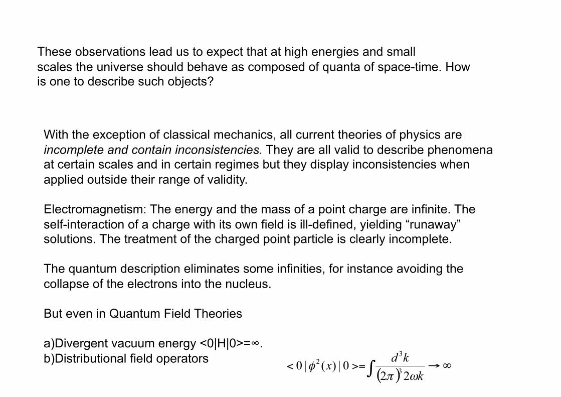
With the exception of classical mechanics, all current theories of physics are incomplete and contain inconsistencies. They are all valid to describe phenomena at certain scales and in certain regimes but they display inconsistencies when applied outside their range of validity.

Electromagnetism: The energy and the mass of a point charge are infinite. The self-interaction of a charge with its own field is ill-defined, yielding “runaway” solutions. The treatment of the charged point particle is clearly incomplete.

The quantum description eliminates some infinities, for instance avoiding the collapse of the electrons into the nucleus.

But even in Quantum Field Theories

a) Divergent vacuum energy <0|H|0>=∞. b) Distributional field operators

These observations lead us to expect that at high energies and small scales the universe should behave as composed of quanta of space-time. How is one to describe such objects?

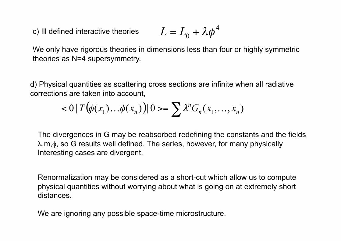
c) Ill defined interactive theories

We only have rigorous theories in dimensions less than four or highly symmetric theories as N=4 supersymmetry.

d) Physical quantities as scattering cross sections are infinite when all radiative corrections are taken into account,

The divergences in G may be reabsorbed redefining the constants and the fields λ,m,φ, so G results well defined. The series, however, for many physically Interesting cases are divergent.

Renormalization may be considered as a short-cut which allow us to compute physical quantities without worrying about what is going on at extremely short distances.

We are ignoring any possible space-time microstructure.

One also has infinities in general relativity.

A generic space-time containing matter will develop singularities in its evolution (Hawking and Penrose singularity theorems).

At a singularity (big bang, black holes) the curvature diverges and matter acquires pathological behaviors. More generally, a space-time is singular if it contains at least one incomplete geodesic.

The geometric description of space-time breaks down at the singularities and only quantum considerations could solve these pathologies.

Summarizing: all known theories of modern physics are partial. Inconsistencies appear when we attempt to apply them beyond their realm of validity.

Only quantum gravity could be complete. It will be relevant at scales when inconsistencies and infinities arise (big bang, black holes singularities, ultra high energy, black hole evaporation).

The problem of unifying quantum mechanics and general relativity is quite complex. Both theories are radically different.

Quantum mechanics in its most developed form, quantum field theory, uses a background space-time in which the notion of particles makes sense. This preferred structure is incompatible with general relativity where space-time is dynamical.

The properties of continuity and differentiability of space-time are essential in general relativity. But in quantum mechanics a quantized space-time is possibly discrete.

We lack experimental evidence of phenomena that are dominated by quantum gravity effects, a theory that becomes relevant in regimes highly difficult to access.

A lot of physicists, motivated by the last observation, have been led to ignore quantum gravity. But ignoring a problem does not make it go away.

We can state that quantum gravity effects are going to be very small, but we do not know how to prove that they actually are (“How do you know the effects of a theory you do not know are small” A. Salam).

The search for consistency:

Searching for consistency in physics has been the source of great discoveries.

Maxwell theory + classical mechanics -> Special Relativity

Special Relativity+ quantum mechanics -> antiparticles, quantum field theory

Special Relativity+ Newtonian gravity -> General Relativity

In all cases progress resulted from taking seriously both points of view and constructing a better synthesis.

Two main approaches:

Canonical quantization and path integral quantization of general relativity-> Loop quantum gravity.

Unification of gravity with other interactions -> string theory.

The existence of more than one approach reflects the state of the art. We still do not have a theory that is completely satisfactory.

General relativity:

Riemannian geometry, a brief review.

Einstein noticed that non inertial systems of reference are locally equivalent to systems in a gravitational field and therefore a theory of gravity will be generally covariant.

General relativity is a theory of gravity but instead of describing the latter as a force, it describes it as a deformation of space-time.

The geometrical properties in a given coordinate system are given by the metric tensor:

Let us recall the properties of a Riemannian geometry in a metric manifold without torsion.

The covariant derivative defines a mapping from (k,l) tensors to (k,l+1) tensors,

The covariant derivative, as a map, has the following properties:

It commutes with the contraction:

On scalars it reduces to the partial derivative:

and due to vanishing torsion:

The previous conditions do not define uniquely the covariant derivative.

with Γ symmetric satisfies the conditions. Under coordinate transformations, Γ transforms in such a way that the covariant derivative of a vector is a (1,1) tensor.

In Riemannian geometries one chooses “metric compatibility”,

Which is convenient because contractions commute with derivatives. A metric compatible derivative with no torsion has a uniquely defined form,

known as the “Christoffel symbols”.

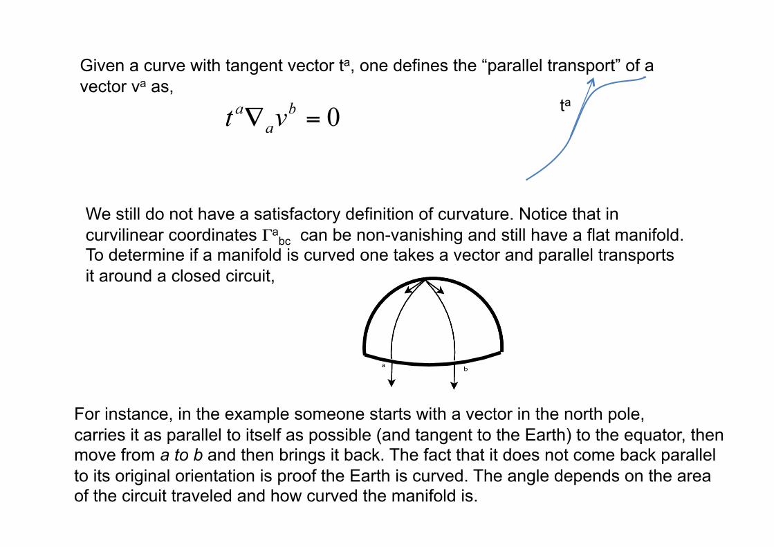
Given a curve with tangent vector ta, one defines the “parallel transport” of a vector va as,

ta

We still do not have a satisfactory definition of curvature. Notice that in curvilinear coordinates Γa

bc can be non-vanishing and still have a flat manifold. To determine if a manifold is curved one takes a vector and parallel transports it around a closed circuit,

For instance, in the example someone starts with a vector in the north pole, carries it as parallel to itself as possible (and tangent to the Earth) to the equator, then move from a to b and then brings it back. The fact that it does not come back parallel to its original orientation is proof the Earth is curved. The angle depends on the area of the circuit traveled and how curved the manifold is.

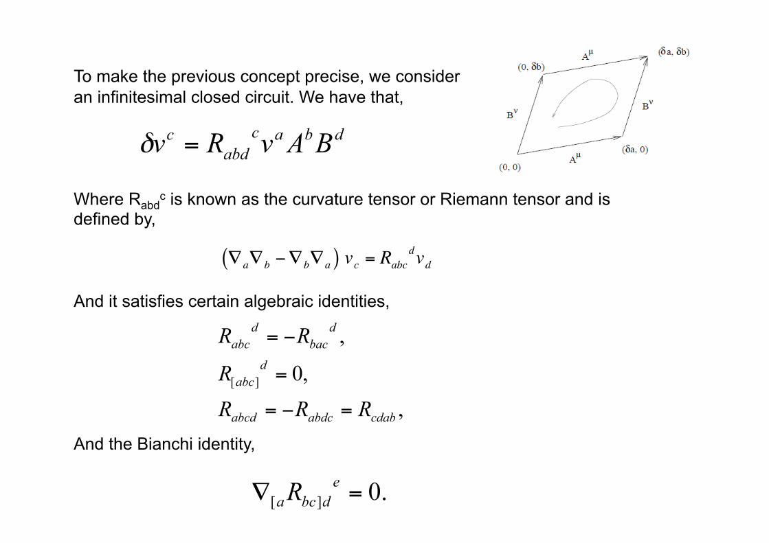
To make the previous concept precise, we consider an infinitesimal closed circuit. We have that,

Where Rabdc is known as the curvature tensor or Riemann tensor and is

defined by,

And it satisfies certain algebraic identities,

And the Bianchi identity,

€

∇a∇b −∇b∇a( ) vc = Rabcdvd

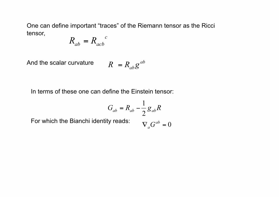
One can define important “traces” of the Riemann tensor as the Ricci tensor,

And the scalar curvature

In terms of these one can define the Einstein tensor:

For which the Bianchi identity reads:

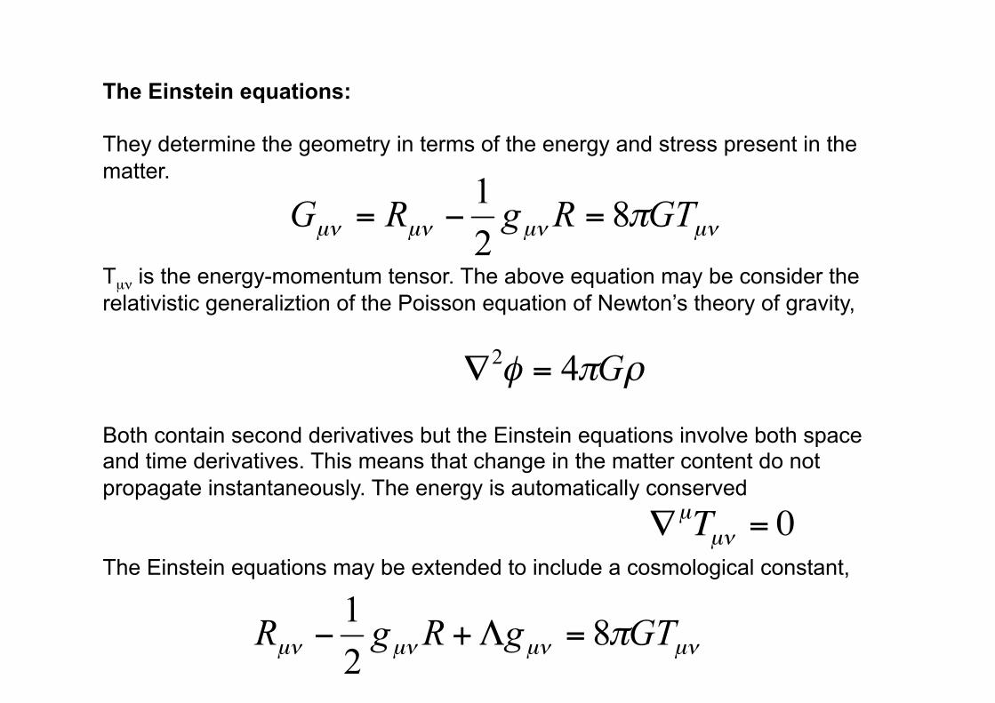
The Einstein equations:

They determine the geometry in terms of the energy and stress present in the matter.

Tµν is the energy-momentum tensor. The above equation may be consider the relativistic generaliztion of the Poisson equation of Newton’s theory of gravity,

Both contain second derivatives but the Einstein equations involve both space and time derivatives. This means that change in the matter content do not propagate instantaneously. The energy is automatically conserved

The Einstein equations may be extended to include a cosmological constant,

€

∇µTµν = 0

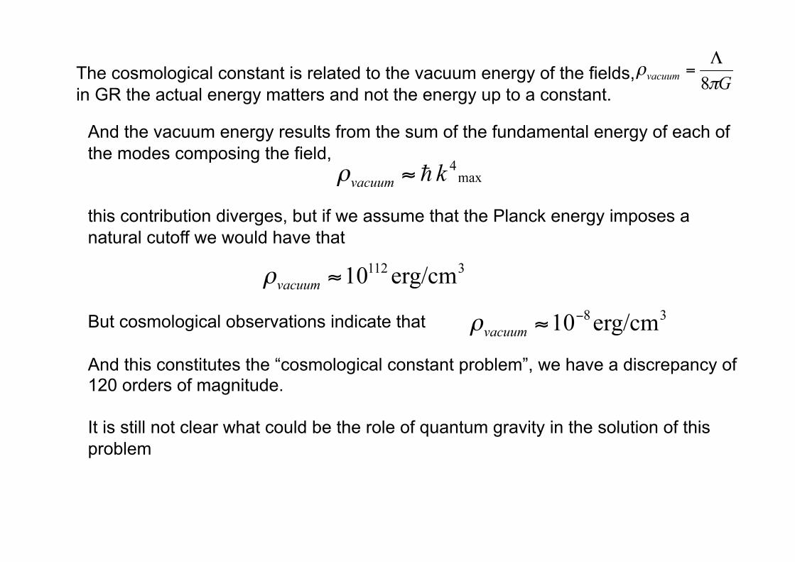
The cosmological constant is related to the vacuum energy of the fields, in GR the actual energy matters and not the energy up to a constant.

And the vacuum energy results from the sum of the fundamental energy of each of the modes composing the field,

this contribution diverges, but if we assume that the Planck energy imposes a natural cutoff we would have that

But cosmological observations indicate that

And this constitutes the “cosmological constant problem”, we have a discrepancy of 120 orders of magnitude.

It is still not clear what could be the role of quantum gravity in the solution of this problem

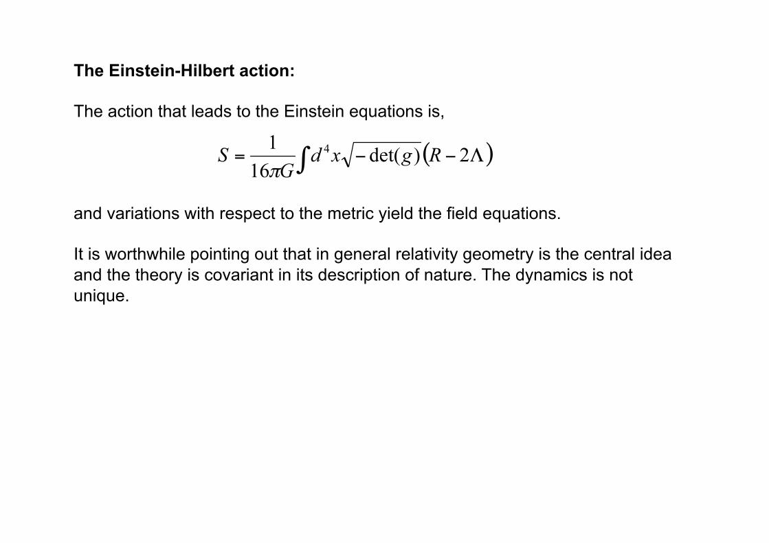
The Einstein-Hilbert action:

The action that leads to the Einstein equations is,

and variations with respect to the metric yield the field equations.

It is worthwhile pointing out that in general relativity geometry is the central idea and the theory is covariant in its description of nature. The dynamics is not unique.

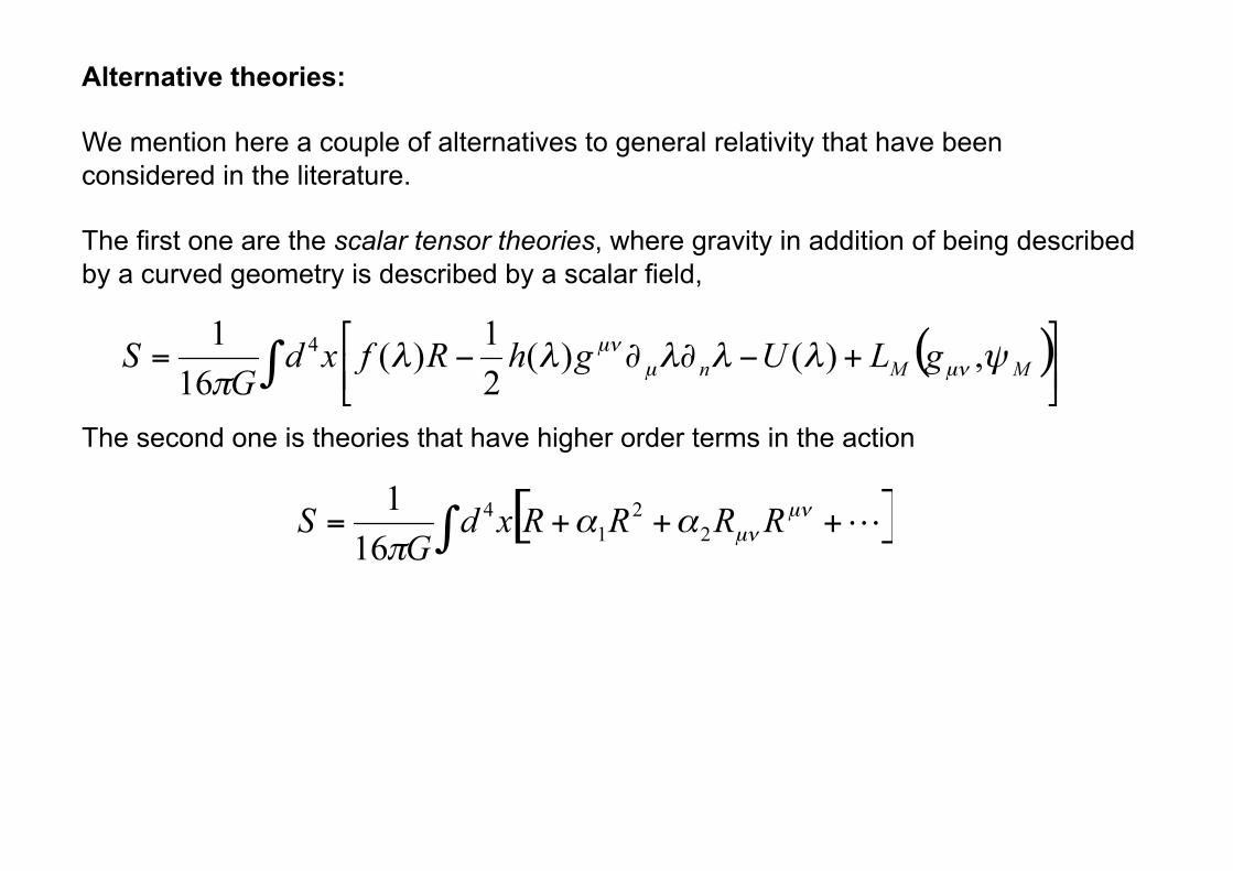
Alternative theories:

We mention here a couple of alternatives to general relativity that have been considered in the literature.

The first one are the scalar tensor theories, where gravity in addition of being described by a curved geometry is described by a scalar field,

The second one is theories that have higher order terms in the action

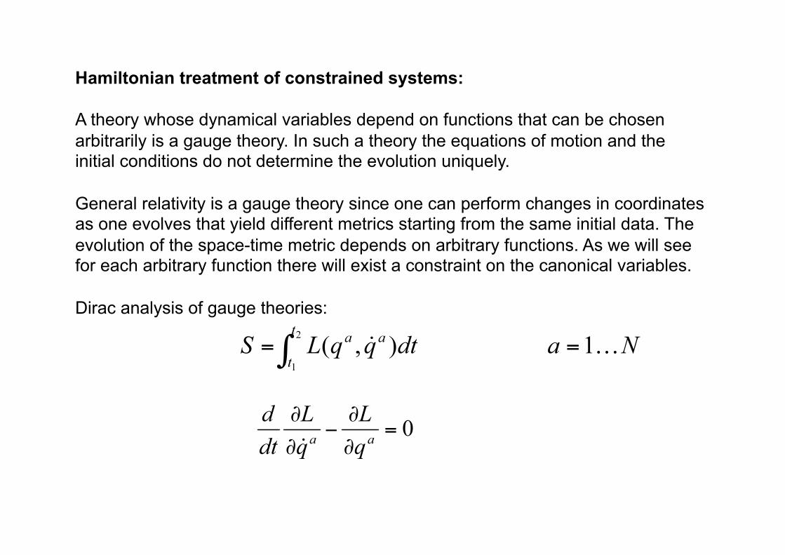
Hamiltonian treatment of constrained systems:

A theory whose dynamical variables depend on functions that can be chosen arbitrarily is a gauge theory. In such a theory the equations of motion and the initial conditions do not determine the evolution uniquely.

General relativity is a gauge theory since one can perform changes in coordinates as one evolves that yield different metrics starting from the same initial data. The evolution of the space-time metric depends on arbitrary functions. As we will see for each arbitrary function there will exist a constraint on the canonical variables.

Dirac analysis of gauge theories:

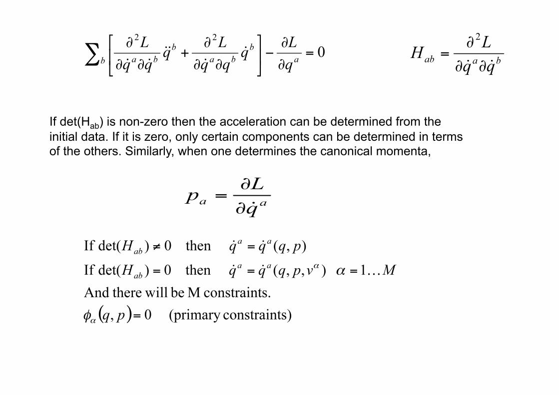
If det(Hab) is non-zero then the acceleration can be determined from the initial data. If it is zero, only certain components can be determined in terms of the others. Similarly, when one determines the canonical momenta,

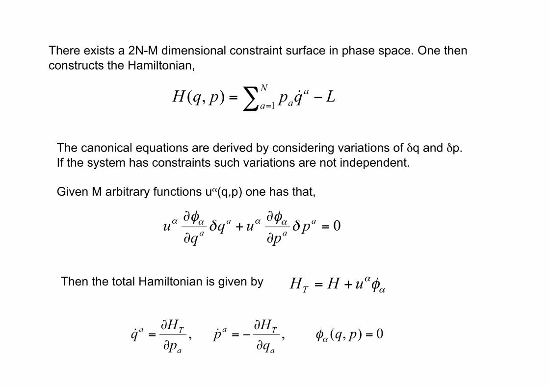
There exists a 2N-M dimensional constraint surface in phase space. One then constructs the Hamiltonian,

The canonical equations are derived by considering variations of δq and δp. If the system has constraints such variations are not independent.

Given M arbitrary functions uα(q,p) one has that,

Then the total Hamiltonian is given by

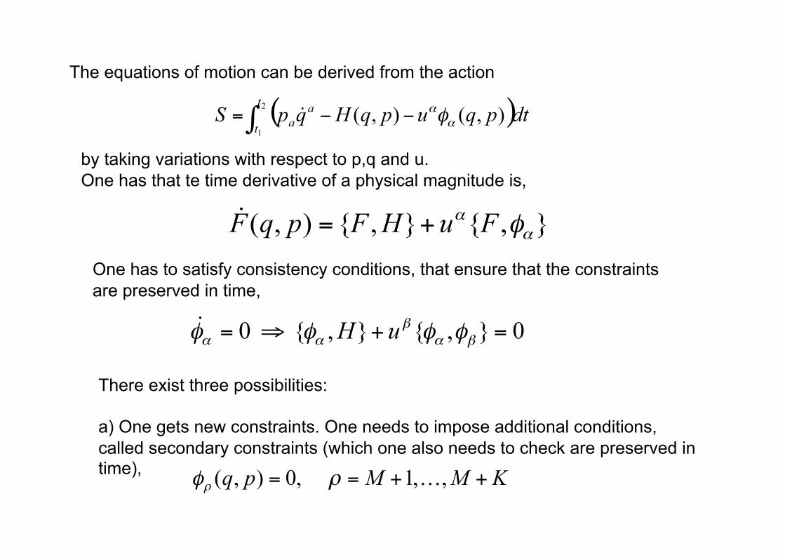
The equations of motion can be derived from the action

by taking variations with respect to p,q and u. One has that te time derivative of a physical magnitude is,

One has to satisfy consistency conditions, that ensure that the constraints are preserved in time,

There exist three possibilities:

a) One gets new constraints. One needs to impose additional conditions, called secondary constraints (which one also needs to check are preserved in time),

b) One gets inconsistencies and the theory does not exist.

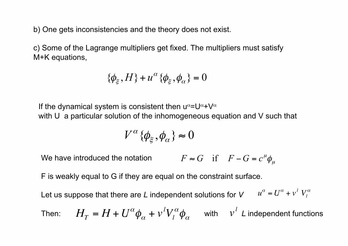
c) Some of the Lagrange multipliers get fixed. The multipliers must satisfy M+K equations,

If the dynamical system is consistent then uα=Uα+Vα

with U a particular solution of the inhomogeneous equation and V such that

We have introduced the notation

F is weakly equal to G if they are equal on the constraint surface.

Let us suppose that there are L independent solutions for V

Then: with L independent functions

€

uα =Uα + v l Vlα

€

HT = H +Uαφα + v lVlαφα

€

€

v l

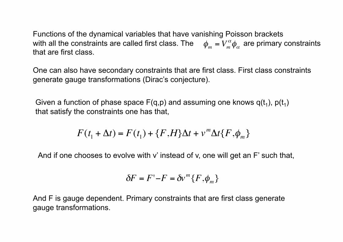
Functions of the dynamical variables that have vanishing Poisson brackets with all the constraints are called first class. The are primary constraints that are first class.

One can also have secondary constraints that are first class. First class constraints generate gauge transformations (Dirac’s conjecture). €

φm =Vmαφα

Given a function of phase space F(q,p) and assuming one knows q(t1), p(t1) that satisfy the constraints one has that,

And if one chooses to evolve with v’ instead of v, one will get an F’ such that,

And F is gauge dependent. Primary constraints that are first class generate gauge transformations.

€

F(t1 + Δt) = F(t1) + {F,H}Δt + vmΔt{F,φm}

€

δF = F '−F = δvm{F,φm}

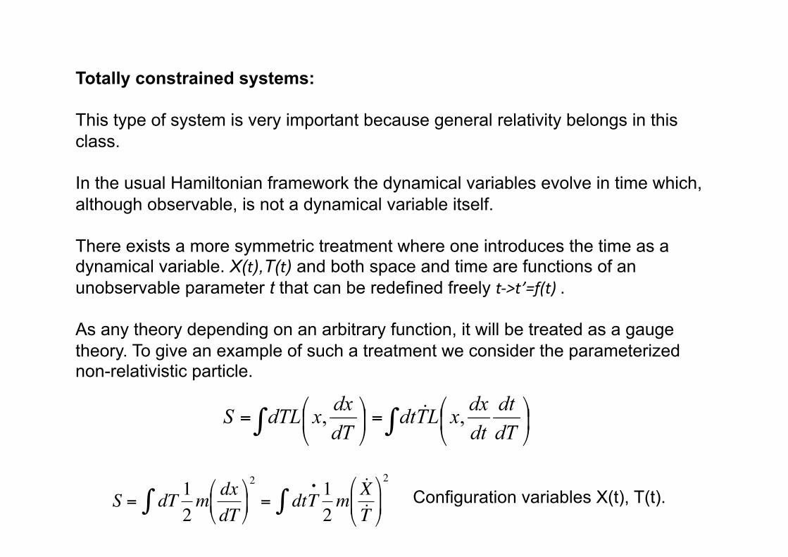
Totally constrained systems:

This type of system is very important because general relativity belongs in this class.

In the usual Hamiltonian framework the dynamical variables evolve in time which, although observable, is not a dynamical variable itself.

There exists a more symmetric treatment where one introduces the time as a dynamical variable. X(t),T(t) and both space and time are functions of an unobservable parameter t that can be redefined freely t‐>t’=f(t).

As any theory depending on an arbitrary function, it will be treated as a gauge theory. To give an example of such a treatment we consider the parameterized non-relativistic particle.

Configuration variables X(t), T(t).

€

S = dT 12

m dxdT

2

= dtT• 1

2m

˙ X ˙ T

2

∫∫

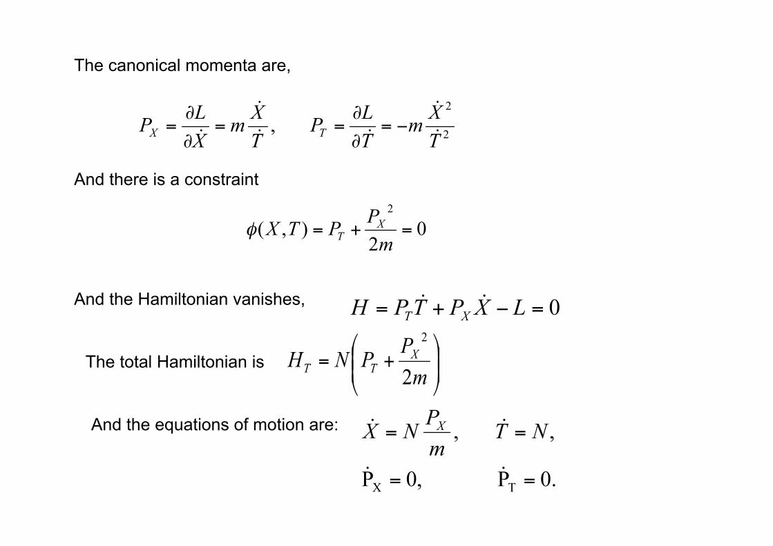
The canonical momenta are,

And there is a constraint

And the Hamiltonian vanishes,

The total Hamiltonian is

And the equations of motion are:

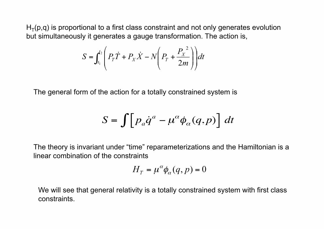
HT(p,q) is proportional to a first class constraint and not only generates evolution but simultaneously it generates a gauge transformation. The action is,

The general form of the action for a totally constrained system is

The theory is invariant under “time” reparameterizations and the Hamiltonian is a linear combination of the constraints

We will see that general relativity is a totally constrained system with first class constraints.

€

S = pa ˙ q a −µαφα (q, p)[ ]∫ dt

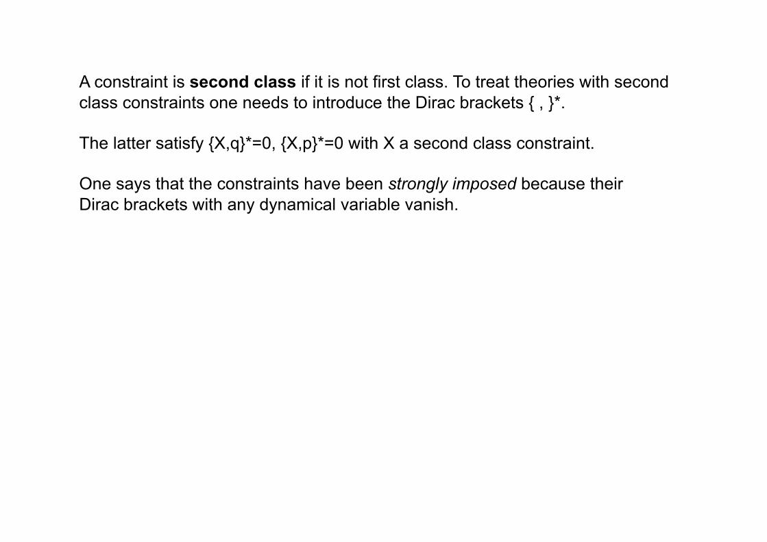
A constraint is second class if it is not first class. To treat theories with second class constraints one needs to introduce the Dirac brackets { , }*.

The latter satisfy {X,q}*=0, {X,p}*=0 with X a second class constraint.

One says that the constraints have been strongly imposed because their Dirac brackets with any dynamical variable vanish.

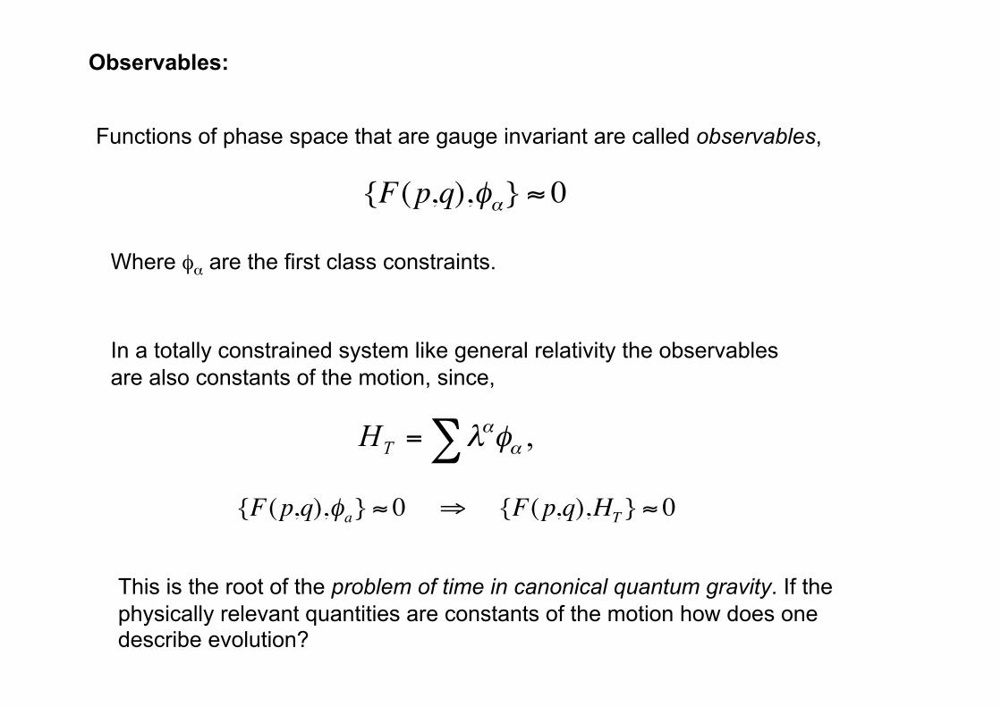
Observables:

Functions of phase space that are gauge invariant are called observables,

Where φα are the first class constraints.

In a totally constrained system like general relativity the observables are also constants of the motion, since,

This is the root of the problem of time in canonical quantum gravity. If the physically relevant quantities are constants of the motion how does one describe evolution? €

{F(p,q),φa} ≈ 0 ⇒ {F(p,q),HT} ≈ 0

€

{F(p,q),φα} ≈ 0

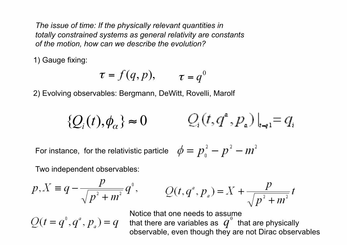
The issue of time: If the physically relevant quantities in totally constrained systems as general relativity are constants of the motion, how can we describe the evolution?

1) Gauge fixing:

2) Evolving observables: Bergmann, DeWitt, Rovelli, Marolf

For instance, for the relativistic particle.

Two independent observables:

Notice that one needs to assume that there are variables as that are physically observable, even though they are not Dirac observables

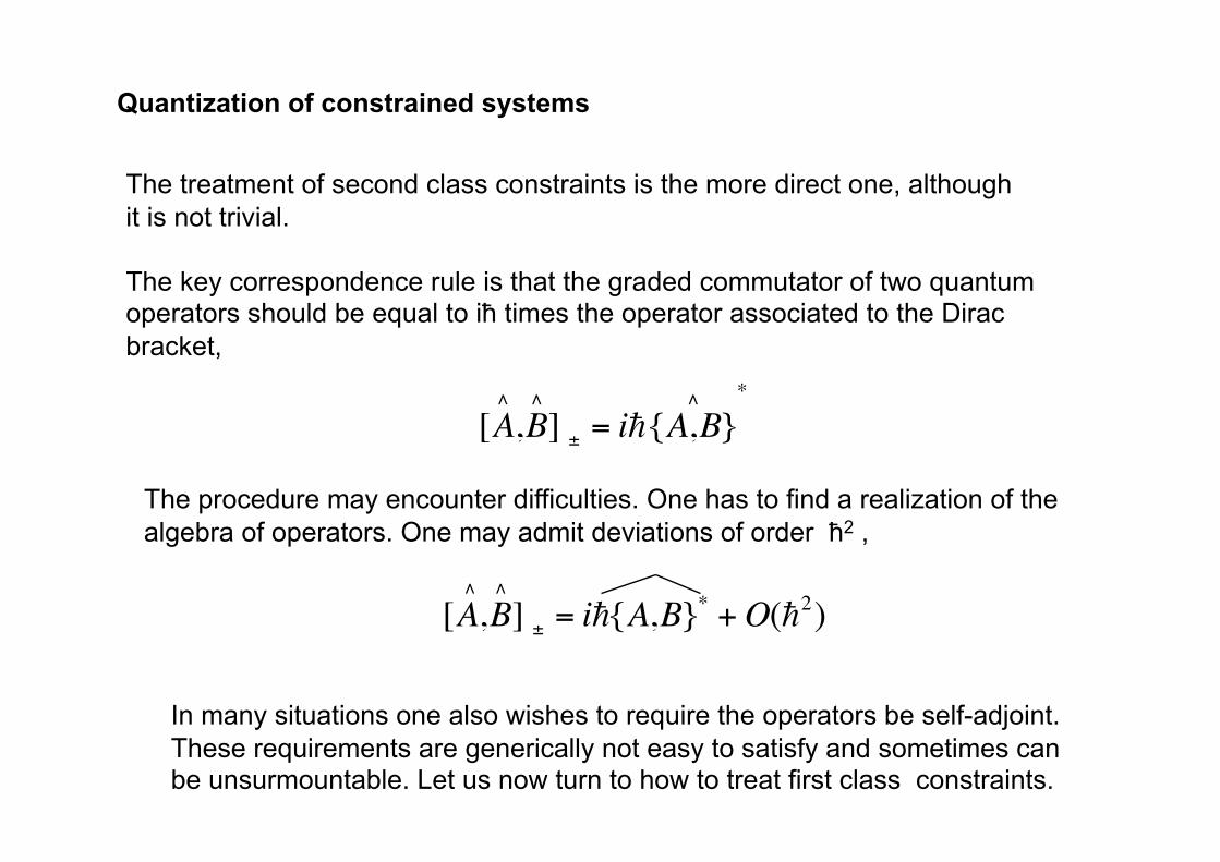
Quantization of constrained systems

The treatment of second class constraints is the more direct one, although it is not trivial.

The key correspondence rule is that the graded commutator of two quantum operators should be equal to iħ times the operator associated to the Dirac bracket,

The procedure may encounter difficulties. One has to find a realization of the algebra of operators. One may admit deviations of order ħ2 ,

In many situations one also wishes to require the operators be self-adjoint. These requirements are generically not easy to satisfy and sometimes can be unsurmountable. Let us now turn to how to treat first class constraints.

€

[A∧

,B∧

] ± = i{A,B}∧ *

€

[A,∧

B∧

] ± = i{A,B}* +O(2)

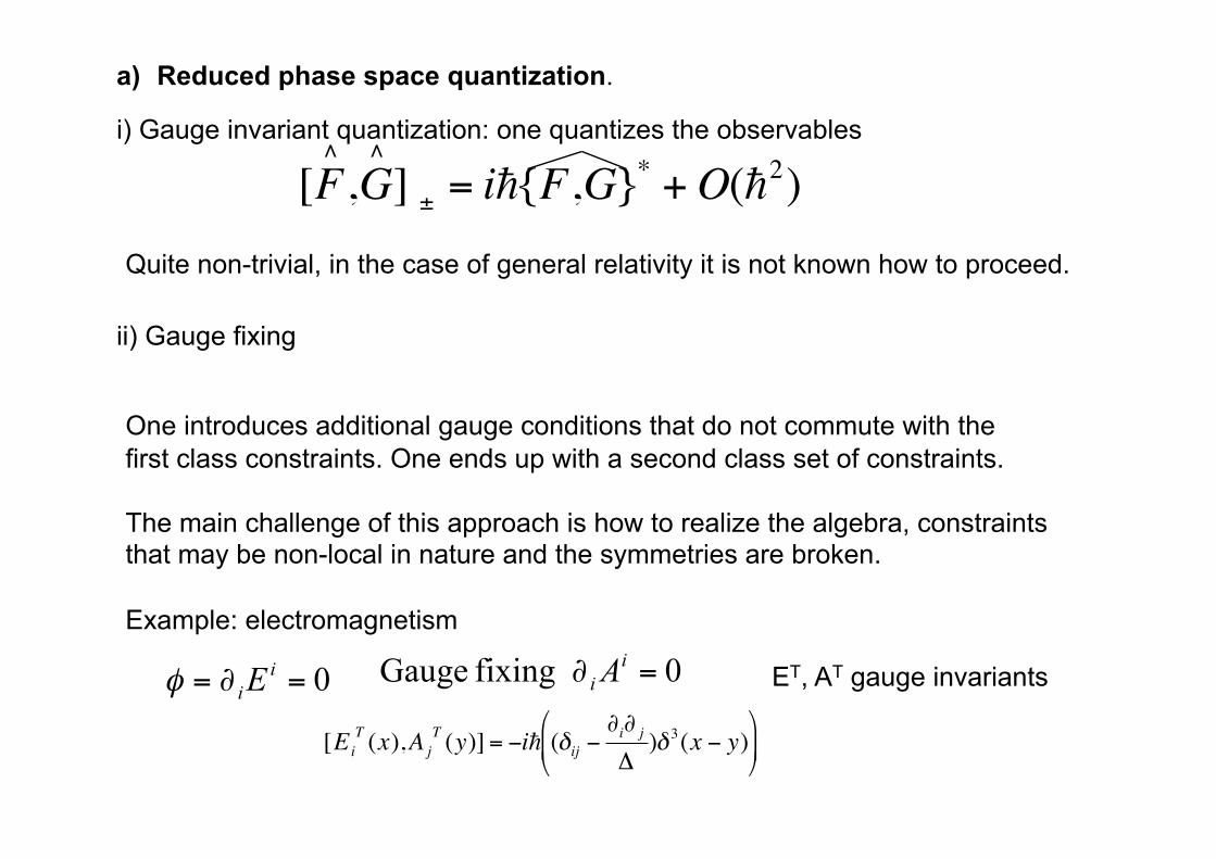
a)  Reduced phase space quantization.

i) Gauge invariant quantization: one quantizes the observables

Quite non-trivial, in the case of general relativity it is not known how to proceed.

ii) Gauge fixing

One introduces additional gauge conditions that do not commute with the first class constraints. One ends up with a second class set of constraints.

The main challenge of this approach is how to realize the algebra, constraints that may be non-local in nature and the symmetries are broken.

Example: electromagnetism

ET, AT gauge invariants

€

[F∧

,G∧

] ± = i{F,G}* +O(2)

€

[EiT (x),A j

T (y)] = −i (δij −∂i∂ j

Δ)δ 3(x − y)

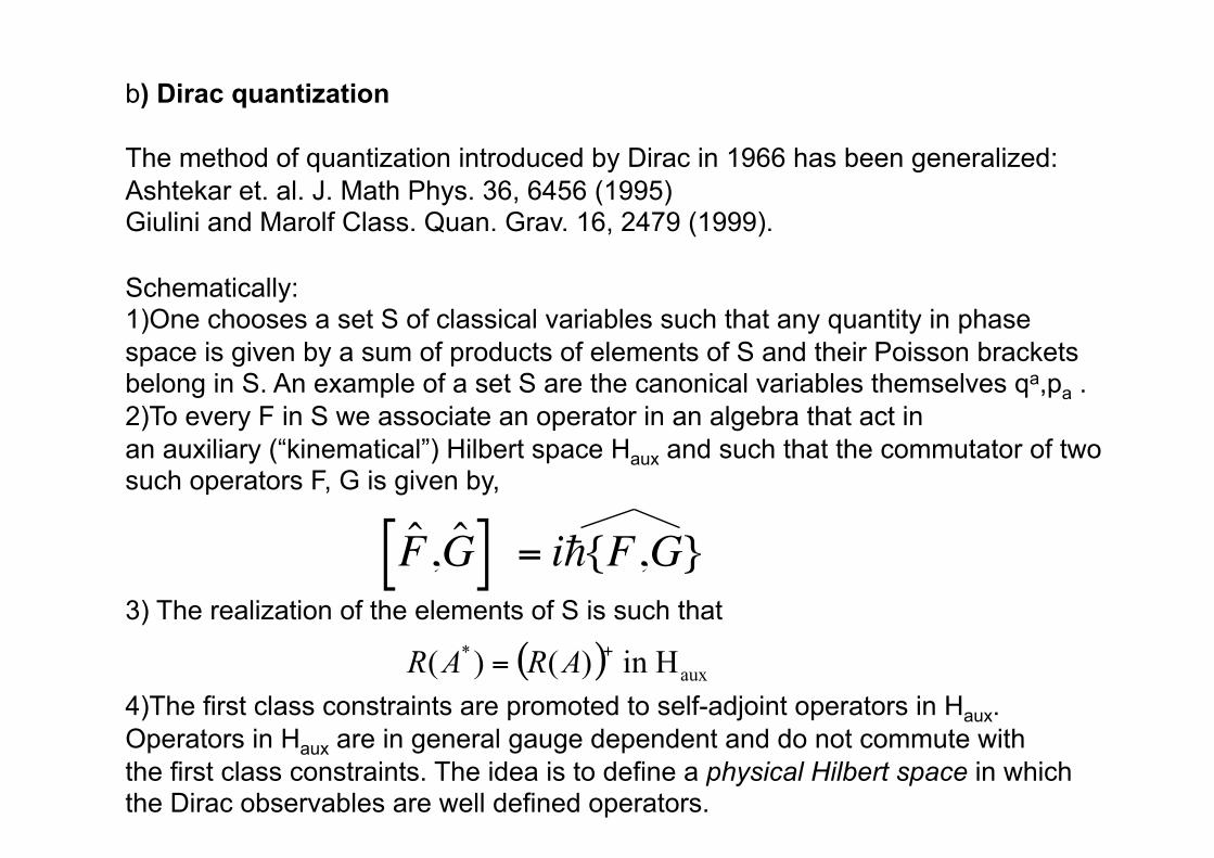
b) Dirac quantization

The method of quantization introduced by Dirac in 1966 has been generalized: Ashtekar et. al. J. Math Phys. 36, 6456 (1995) Giulini and Marolf Class. Quan. Grav. 16, 2479 (1999).

Schematically: 1) One chooses a set S of classical variables such that any quantity in phase space is given by a sum of products of elements of S and their Poisson brackets belong in S. An example of a set S are the canonical variables themselves qa,pa . 2) To every F in S we associate an operator in an algebra that act in an auxiliary (“kinematical”) Hilbert space Haux and such that the commutator of two such operators F, G is given by,

3) The realization of the elements of S is such that

4) The first class constraints are promoted to self-adjoint operators in Haux. Operators in Haux are in general gauge dependent and do not commute with the first class constraints. The idea is to define a physical Hilbert space in which the Dirac observables are well defined operators.

€

ˆ F , ˆ G [ ] = i{F,G}

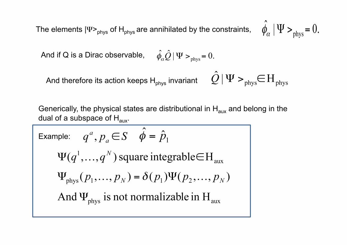
The elements |Ψ>phys of Hphys are annihilated by the constraints,

And if Q is a Dirac observable,

And therefore its action keeps Hphys invariant

Generically, the physical states are distributional in Haux and belong in the dual of a subspace of Haux.

Example:

The Algebraic Quantization procedure (group averaging) for the construction of an inner product in the physical Hilbert space leads to,

And the procedure also ensures that the observables are self-adjoint.

Difficulties with the algebraic quantization procedure:

But at a quantum level one may encounter corrections:

And the original invariances may be lost unless the operator Dαβ annihilates the elements of |Ψ>phys. The additional terms are known as gauge anomalies.

Finally, the group averaging technique used to define the inner product does not always work. Some constraints are not group generators.

€

<ϕ |ψ >phys= dp1dpNδ(p1)∫ ϕ*(p2,…, pN )ψ(p2,…, pN )

€

[φ∧

α ,φ∧

β ] = iCαβγ ˆ φ γ + 2 ˆ D αβ

Consistency

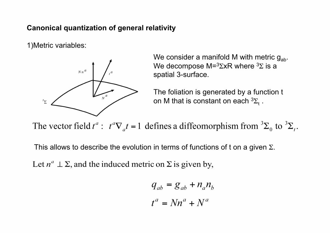
Canonical quantization of general relativity

1) Metric variables: We consider a manifold M with metric gab. We decompose M=3ΣxR where 3Σ is a spatial 3-surface.

The foliation is generated by a function t on M that is constant on each 3Σt .

This allows to describe the evolution in terms of functions of t on a given Σ.

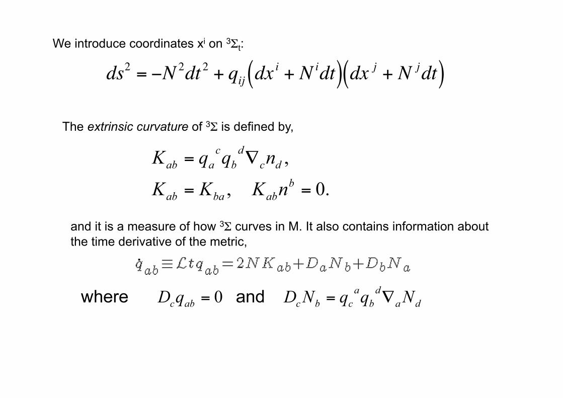
We introduce coordinates xi on 3Σt:

The extrinsic curvature of 3Σ is defined by,

and it is a measure of how 3Σ curves in M. It also contains information about the time derivative of the metric,

€

ds2 = −N 2dt 2 + qij dxi + N idt( ) dx j + N jdt( )

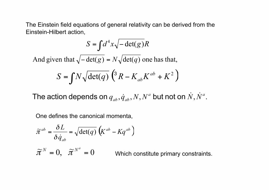
The Einstein field equations of general relativity can be derived from the Einstein-Hilbert action,

One defines the canonical momenta,

Which constitute primary constraints.

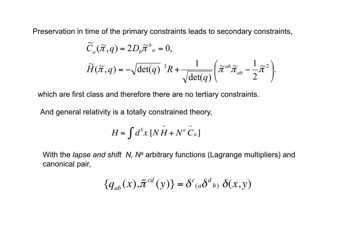
Preservation in time of the primary constraints leads to secondary constraints,

And general relativity is a totally constrained theory,

With the lapse and shift N, Na arbitrary functions (Lagrange multipliers) and canonical pair,

which are first class and therefore there are no tertiary constraints.

€

H = d3x [NH~

∫ + Na C~a ]

€

{qab (x), ˜ π cd (y)} = δ c(aδ d b ) δ(x,y)

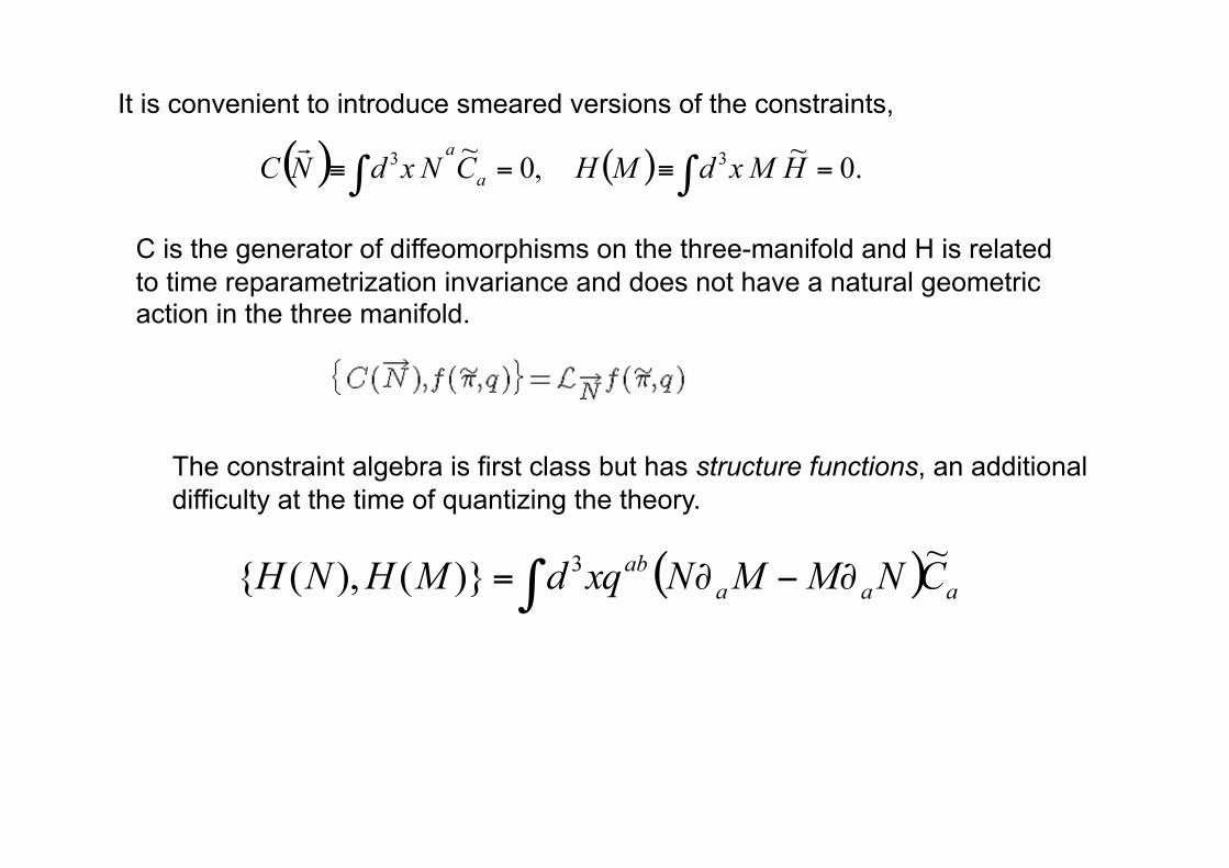
It is convenient to introduce smeared versions of the constraints,

C is the generator of diffeomorphisms on the three-manifold and H is related to time reparametrization invariance and does not have a natural geometric action in the three manifold.

The constraint algebra is first class but has structure functions, an additional difficulty at the time of quantizing the theory.

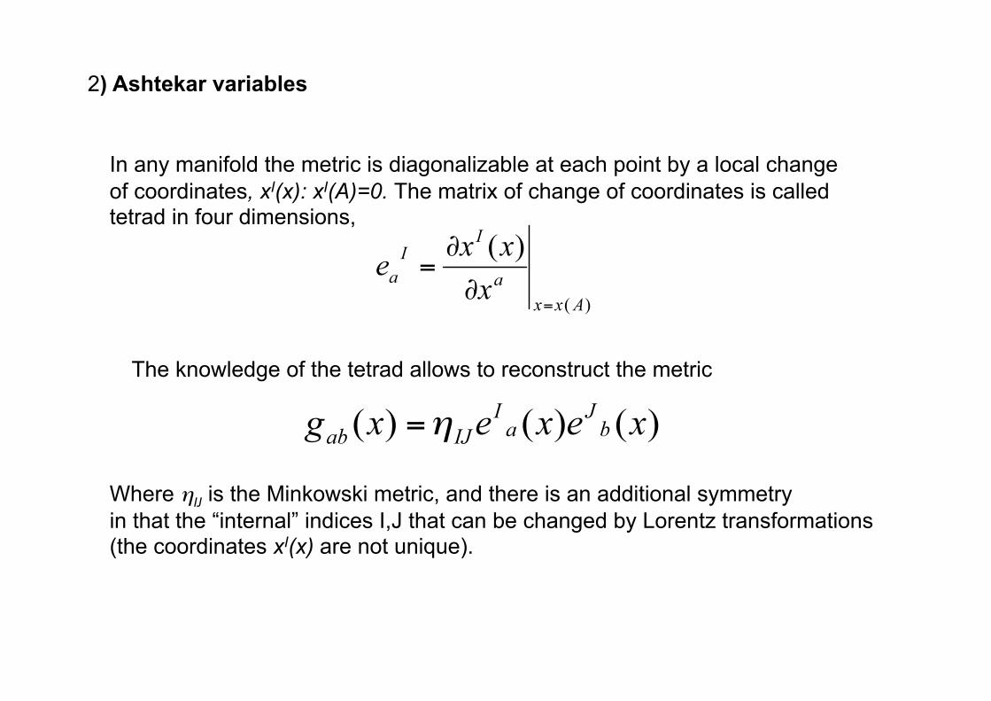
2) Ashtekar variables

In any manifold the metric is diagonalizable at each point by a local change of coordinates, xI(x): xI(A)=0. The matrix of change of coordinates is called tetrad in four dimensions,

The knowledge of the tetrad allows to reconstruct the metric

Where ηIJ is the Minkowski metric, and there is an additional symmetry in that the “internal” indices I,J that can be changed by Lorentz transformations (the coordinates xI(x) are not unique).

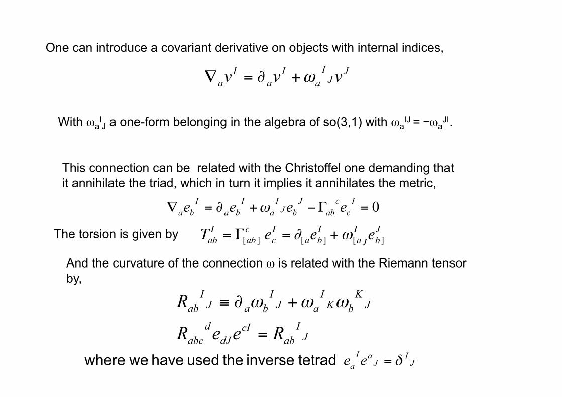
One can introduce a covariant derivative on objects with internal indices,

With ωaIJ a one-form belonging in the algebra of so(3,1) with ωa

IJ = -ωaJI.

This connection can be related with the Christoffel one demanding that it annihilate the triad, which in turn it implies it annihilates the metric,

And the curvature of the connection ω is related with the Riemann tensor by,

The torsion is given by

€

TabI = Γ[ab ]

c ecI = ∂[aeb ]

I +ω[aIJeb ]

J

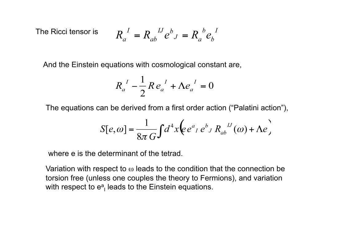
The Ricci tensor is

And the Einstein equations with cosmological constant are,

The equations can be derived from a first order action (“Palatini action”),

Variation with respect to ω leads to the condition that the connection be torsion free (unless one couples the theory to Fermions), and variation with respect to ea

I leads to the Einstein equations.

where e is the determinant of the tetrad.

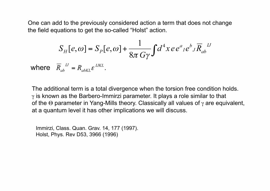
One can add to the previously considered action a term that does not change the field equations to get the so-called “Holst” action.

The additional term is a total divergence when the torsion free condition holds. γ is known as the Barbero-Immirzi parameter. It plays a role similar to that of the Θ parameter in Yang-Mills theory. Classically all values of γ are equivalent, at a quantum level it has other implications we will discuss.

Immirzi, Class. Quan. Grav. 14, 177 (1997). Holst, Phys. Rev D53, 3966 (1996)

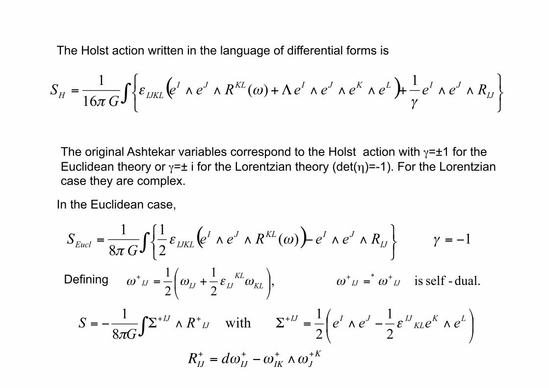
The Holst action written in the language of differential forms is

The original Ashtekar variables correspond to the Holst action with γ=±1 for the Euclidean theory or γ=± i for the Lorentzian theory (det(η)=-1). For the Lorentzian case they are complex.

In the Euclidean case,

Defining

€

RIJ+ = dω IJ

+ −ω IK+ ∧ωJ

+K

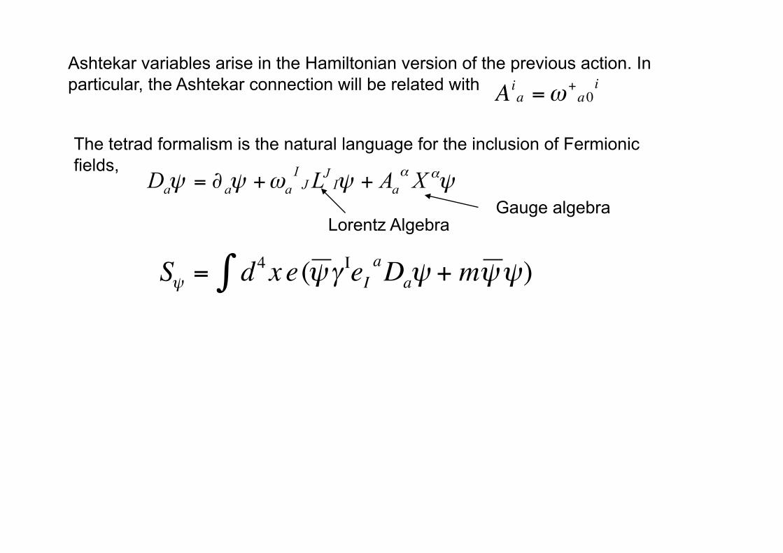
Ashtekar variables arise in the Hamiltonian version of the previous action. In particular, the Ashtekar connection will be related with

The tetrad formalism is the natural language for the inclusion of Fermionic fields,

Lorentz Algebra Gauge algebra

€

Sψ = d4x e(ψ γΙeIaDaψ + mψ ψ)∫

€

Aia =ω +

a0i

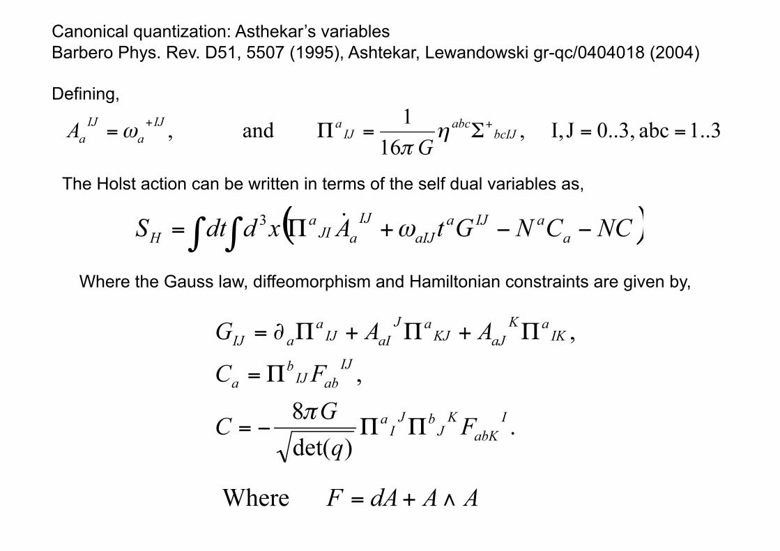
Canonical quantization: Asthekar’s variables Barbero Phys. Rev. D51, 5507 (1995), Ashtekar, Lewandowski gr-qc/0404018 (2004)

Defining,

The Holst action can be written in terms of the self dual variables as,

Where the Gauss law, diffeomorphism and Hamiltonian constraints are given by,

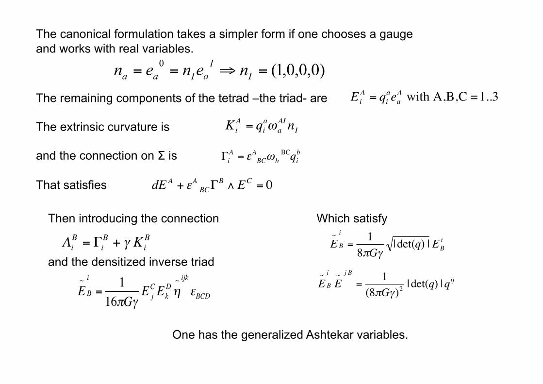
The canonical formulation takes a simpler form if one chooses a gauge and works with real variables.

The remaining components of the tetrad –the triad- are

The extrinsic curvature is

and the connection on Σ is

That satisfies

€

EiA = qi

aeaA with A,B,C =1..3

€

KiA = qi

aωaAI nI

€

ΓiA = ε BC

A ωb BCqi

b

€

dE A + ε BCA ΓB ∧ EC = 0

Then introducing the connection

and the densitized inverse triad

€

AiB = Γi

B + γ KiB

€

E~B

i

=1

16πGγE jC Ek

Dη~ ijk

εBCD

Which satisfy

€

E~B

i

=1

8πGγ| det(q) | EB

i

€

E~B

i

E~ j B

=1

(8πGγ)2 | det(q) |qij

One has the generalized Ashtekar variables.

€

{AaB (x),E

~A

b

(y)} = δabδA

Bδ(x,y)

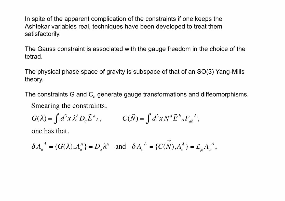
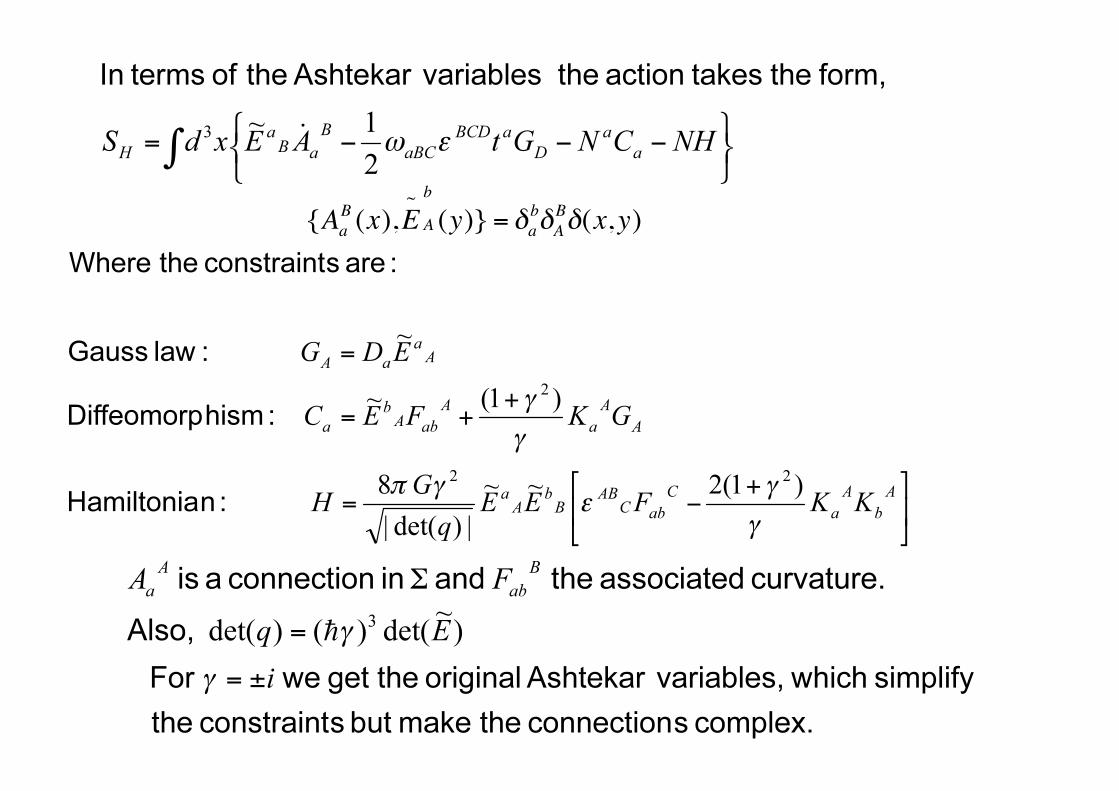
In spite of the apparent complication of the constraints if one keeps the Ashtekar variables real, techniques have been developed to treat them satisfactorily.

The Gauss constraint is associated with the gauge freedom in the choice of the tetrad.

The physical phase space of gravity is subspace of that of an SO(3) Yang-Mills theory.

The constraints G and Ca generate gauge transformations and diffeomorphisms.

€

Smearing the constraints,

G(λ) = d3x λA∫ Da˜ E a A , C(

N ) = d3x N a∫ ˜ E b A Fab

A ,

one has that,

δ AaA = {G(λ),Aa

A } = DaλA and δ Aa

A = {C(N→

), AaA } = L

N Aa

A ,

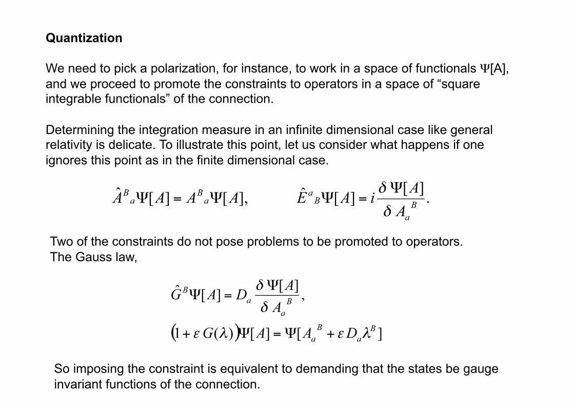
Quantization

We need to pick a polarization, for instance, to work in a space of functionals Ψ[A], and we proceed to promote the constraints to operators in a space of “square integrable functionals” of the connection.

Determining the integration measure in an infinite dimensional case like general relativity is delicate. To illustrate this point, let us consider what happens if one ignores this point as in the finite dimensional case.

Two of the constraints do not pose problems to be promoted to operators. The Gauss law,

So imposing the constraint is equivalent to demanding that the states be gauge invariant functions of the connection.

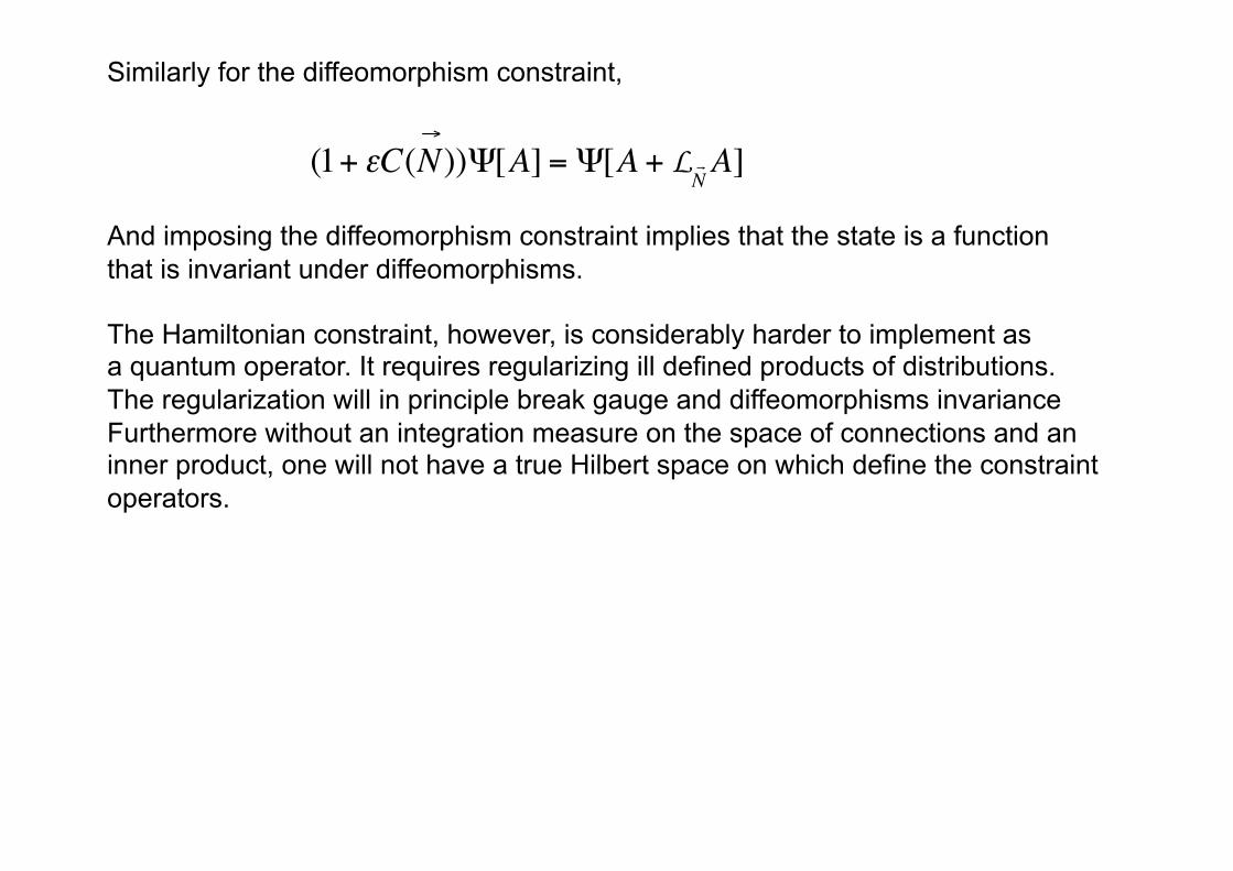
Similarly for the diffeomorphism constraint,

€

(1+ εC(N→

))Ψ[A] = Ψ[A + L N

A]

And imposing the diffeomorphism constraint implies that the state is a function that is invariant under diffeomorphisms.

The Hamiltonian constraint, however, is considerably harder to implement as a quantum operator. It requires regularizing ill defined products of distributions. The regularization will in principle break gauge and diffeomorphisms invariance Furthermore without an integration measure on the space of connections and an inner product, one will not have a true Hilbert space on which define the constraint operators.

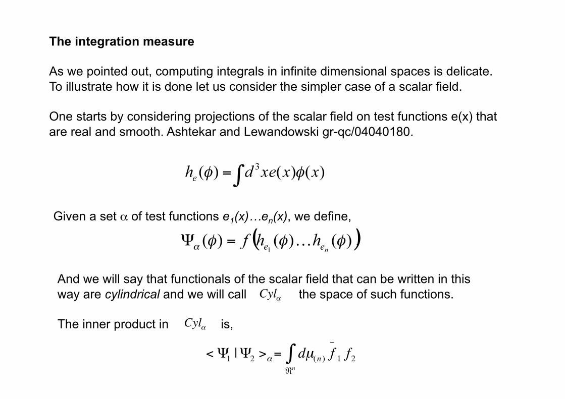
The integration measure

As we pointed out, computing integrals in infinite dimensional spaces is delicate. To illustrate how it is done let us consider the simpler case of a scalar field.

One starts by considering projections of the scalar field on test functions e(x) that are real and smooth. Ashtekar and Lewandowski gr-qc/04040180.

Given a set α of test functions e1(x)…en(x), we define,

And we will say that functionals of the scalar field that can be written in this way are cylindrical and we will call the space of such functions.

The inner product in is,

€

Cylα

€

Cylα

€

< Ψ1 |Ψ2 >α= dµ(n ) f−

1 f2ℜn

∫

The idea is to go from Cylα to Cyl, the space of cylindrical functions defined for some α.

To do this one needs to show that Ψ is cylindrical for two different sets α and β. There exist consistent measures µ(n) that yield the same result. It can be shown that the Gaussian measures are good for this purpose.

The idea is to include in the Hilbert space states that are limits of Cauchy sequences of normalizable cylindrical states.

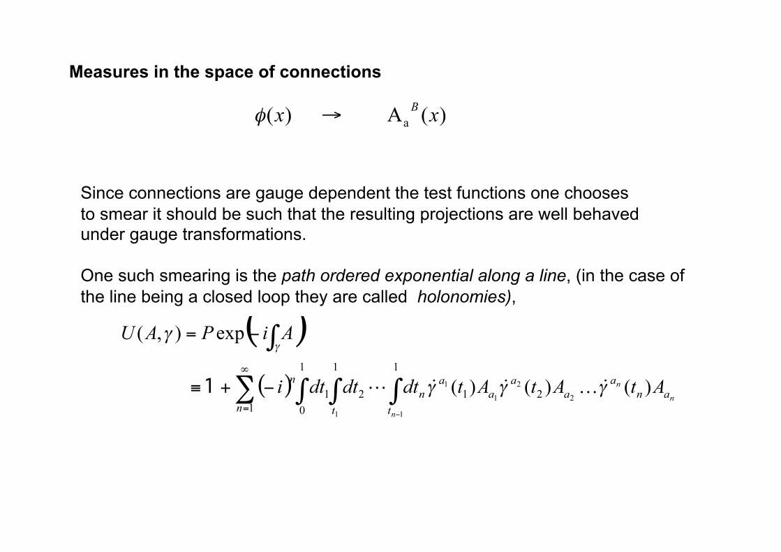
Measures in the space of connections

Since connections are gauge dependent the test functions one chooses to smear it should be such that the resulting projections are well behaved under gauge transformations.

One such smearing is the path ordered exponential along a line, (in the case of the line being a closed loop they are called holonomies),

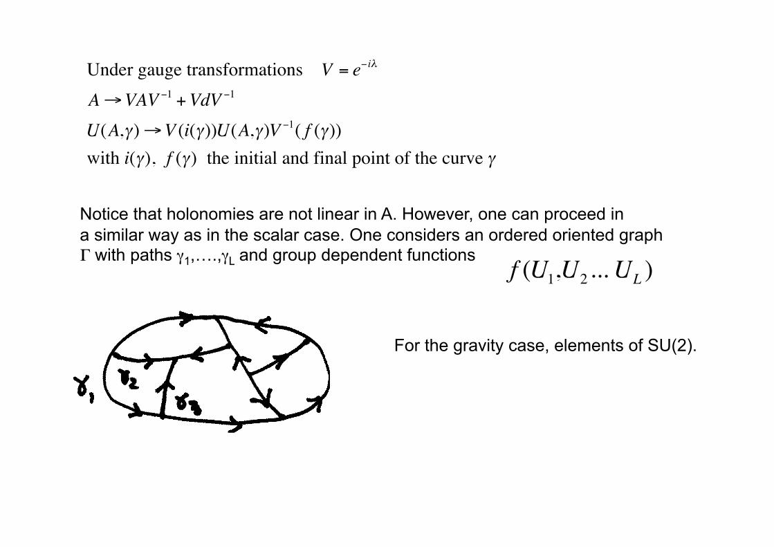
Notice that holonomies are not linear in A. However, one can proceed in a similar way as in the scalar case. One considers an ordered oriented graph Γ with paths γ1,….,γL and group dependent functions

€

Under gauge transformations V = e−iλ

A→VAV −1 +VdV −1

U(A,γ)→V (i(γ))U(A,γ)V −1( f (γ))with i(γ), f (γ) the initial and final point of the curve γ

€ €

f (U1,U2 ... UL )

For the gravity case, elements of SU(2).

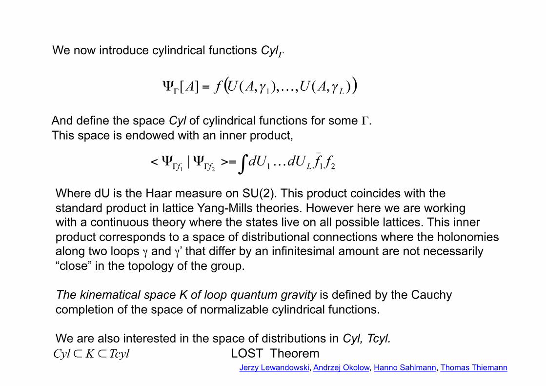
We now introduce cylindrical functions CylΓ

And define the space Cyl of cylindrical functions for some Γ. This space is endowed with an inner product,

Where dU is the Haar measure on SU(2). This product coincides with the standard product in lattice Yang-Mills theories. However here we are working with a continuous theory where the states live on all possible lattices. This inner product corresponds to a space of distributional connections where the holonomies along two loops γ and γ’ that differ by an infinitesimal amount are not necessarily “close” in the topology of the group.

The kinematical space Κ of loop quantum gravity is defined by the Cauchy completion of the space of normalizable cylindrical functions.

We are also interested in the space of distributions in Cyl, Tcyl.

Jerzy Lewandowski, Andrzej Okolow, Hanno Sahlmann, Thomas Thiemann

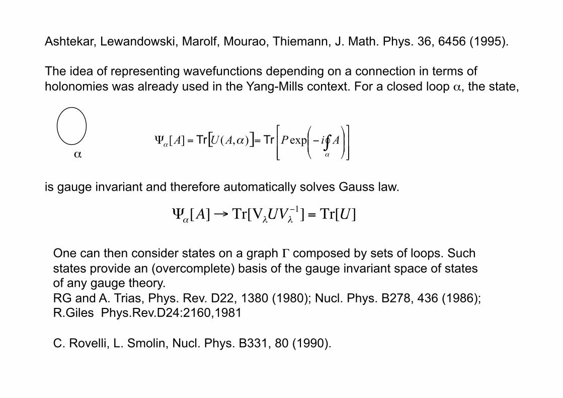
Ashtekar, Lewandowski, Marolf, Mourao, Thiemann, J. Math. Phys. 36, 6456 (1995).

The idea of representing wavefunctions depending on a connection in terms of holonomies was already used in the Yang-Mills context. For a closed loop α, the state,

α

is gauge invariant and therefore automatically solves Gauss law.

One can then consider states on a graph Γ composed by sets of loops. Such states provide an (overcomplete) basis of the gauge invariant space of states of any gauge theory. RG and A. Trias, Phys. Rev. D22, 1380 (1980); Nucl. Phys. B278, 436 (1986); R.Giles Phys.Rev.D24:2160,1981

C. Rovelli, L. Smolin, Nucl. Phys. B331, 80 (1990).

€

Ψα[A]→ Tr[VλUVλ−1] = Tr[U]

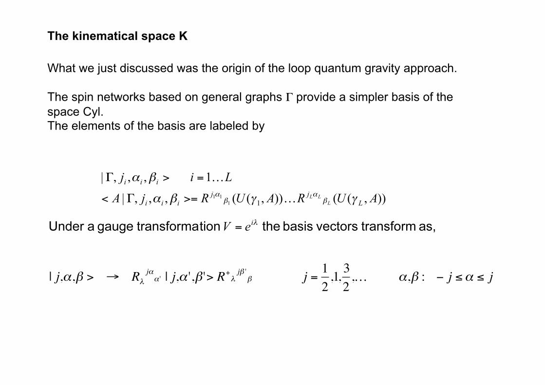
The kinematical space K

What we just discussed was the origin of the loop quantum gravity approach.

The spin networks based on general graphs Γ provide a simpler basis of the space Cyl. The elements of the basis are labeled by

€

| j,α,β > → Rλjαα ' | j,α ',β '> R+

λjβ '

β j =12

,1, 32

,… α,β : − j ≤α ≤ j

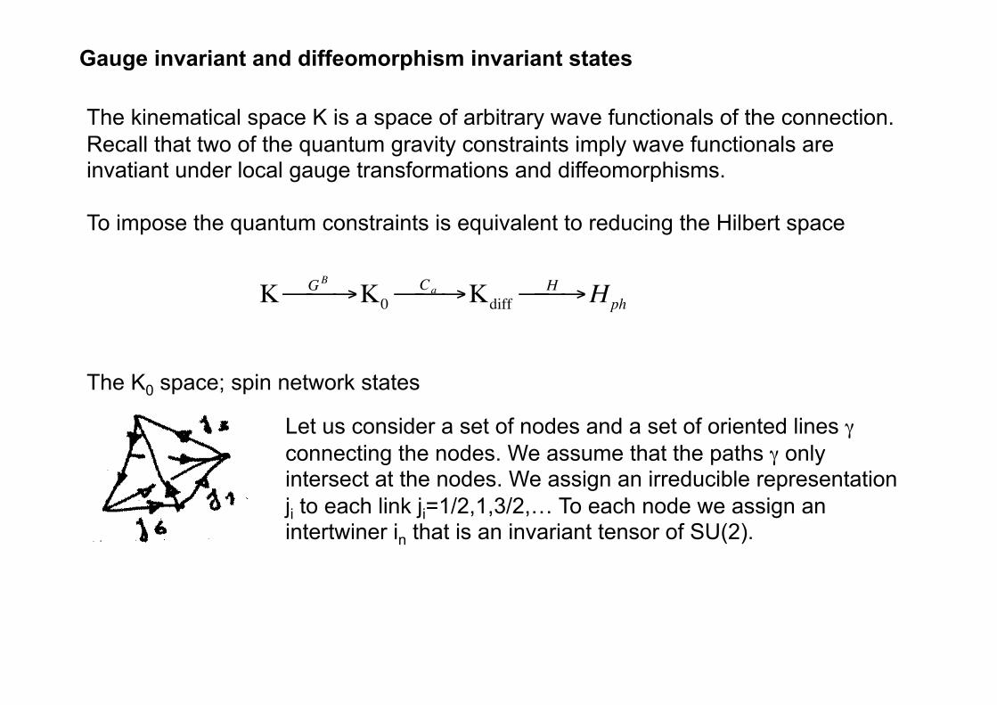
Gauge invariant and diffeomorphism invariant states

The kinematical space K is a space of arbitrary wave functionals of the connection. Recall that two of the quantum gravity constraints imply wave functionals are invatiant under local gauge transformations and diffeomorphisms.

To impose the quantum constraints is equivalent to reducing the Hilbert space

The K0 space; spin network states

Let us consider a set of nodes and a set of oriented lines γ connecting the nodes. We assume that the paths γ only intersect at the nodes. We assign an irreducible representation ji to each link ji=1/2,1,3/2,… To each node we assign an intertwiner in that is an invariant tensor of SU(2).

€

Κ GB

→ Κ0Ca → Κdiff

H → Hph

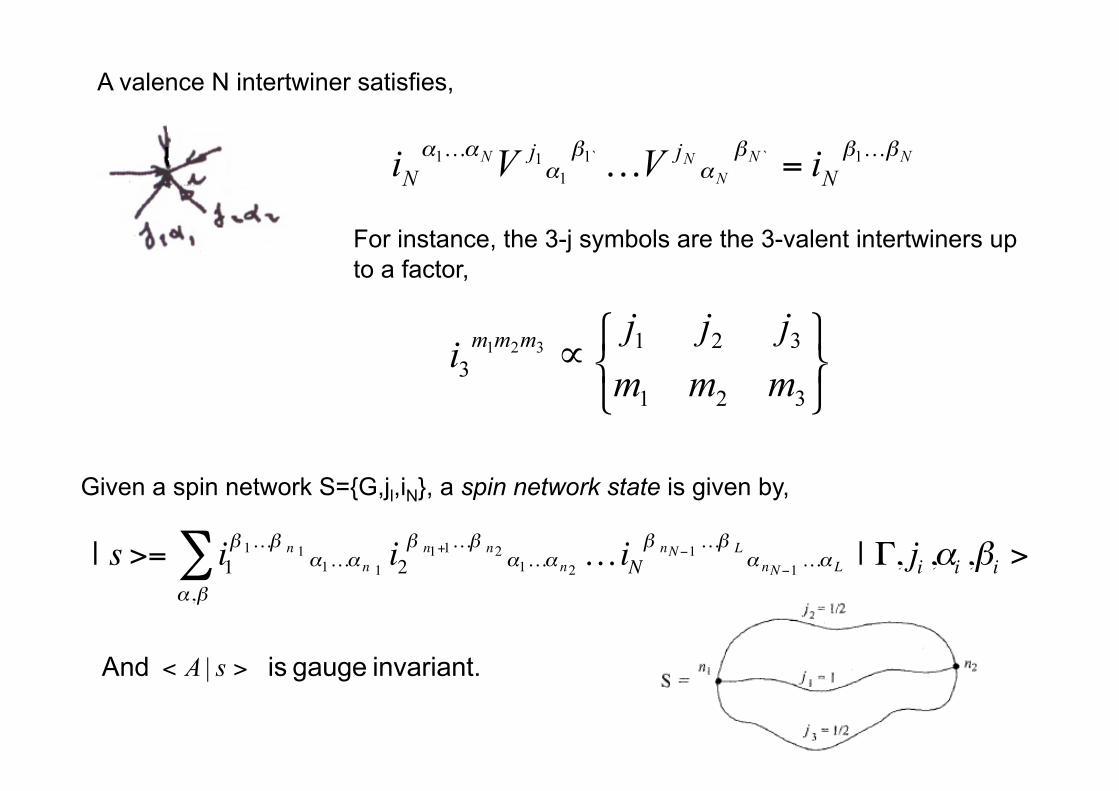
A valence N intertwiner satisfies,

For instance, the 3-j symbols are the 3-valent intertwiners up to a factor,

Given a spin network S={G,jl,iN}, a spin network state is given by,

€

| s >= i1β 1…β n 1 α1…α n 1

i2β n1+1…β n2 α1…α n2

…iNβ nN−1 …β L

α nN−1 …α L | Γ, ji ,αi ,βi >α ,β∑

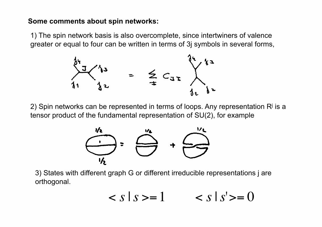
Some comments about spin networks:

1) The spin network basis is also overcomplete, since intertwiners of valence greater or equal to four can be written in terms of 3j symbols in several forms,

2) Spin networks can be represented in terms of loops. Any representation Rj is a tensor product of the fundamental representation of SU(2), for example

3) States with different graph G or different irreducible representations j are orthogonal.

€

< s | s >=1 < s | s'>= 0

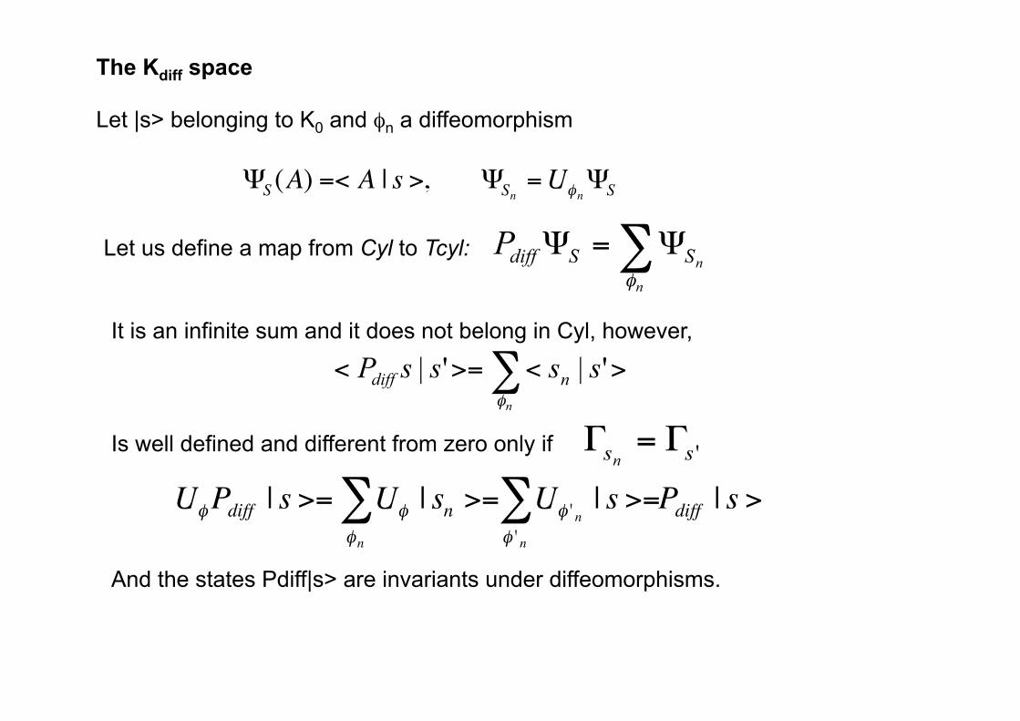
The Kdiff space

Let |s> belonging to K0 and φn a diffeomorphism

Let us define a map from Cyl to Tcyl:

It is an infinite sum and it does not belong in Cyl, however,

Is well defined and different from zero only if

€

UφPdiff | s >= Uφ | sn >=φn

∑ Uφ 'n| s >=

φ 'n

∑ Pdiff | s >

And the states Pdiff|s> are invariants under diffeomorphisms.

€

ΨS (A) =< A | s >, ΨSn=Uφn

ΨS

The elements of Kdiff given by Pdiff |s> are not in a subspace of K0, they are distributional on K0. The inner product is given by,

The elements of Kdiff are “spin knots”

This concludes the construction of the kinematical space of loop quantum gravity. In order to gain some insight into the geometric meaning of the states we will introduce operators associated with the geometry.

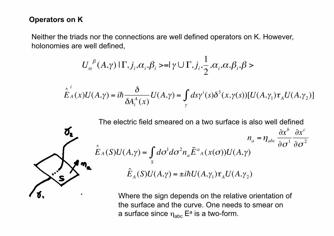
Operators on K

Neither the triads nor the connections are well defined operators on K. However, holonomies are well defined,

The electric field smeared on a two surface is also well defined

€

E∧

A (S)U(A,γ) = dσ1

S∫ dσ 2na

˜ E a A (x(σ))U(A,γ)

Where the sign depends on the relative orientation of the surface and the curve. One needs to smear on a surface since ηabc Ea is a two-form.

€

Uαβ (A,γ) |Γ, ji,α i,βi >=| γ ∪Γ, ji,

12,α i,α,β i,β >

€

ˆ E A (S)U(A,γ) = ±iU(A,γ1)τAU(A,γ 2)

€

E∧

A

i

(x)U(A,γ) = i δδAi

A (x)U(A,γ) = dsγ i(s)δ 3(x,γ(s))[U(A,γ1)τAU(A,γ 2)]

γ

∫

Geometric operators on Κ0

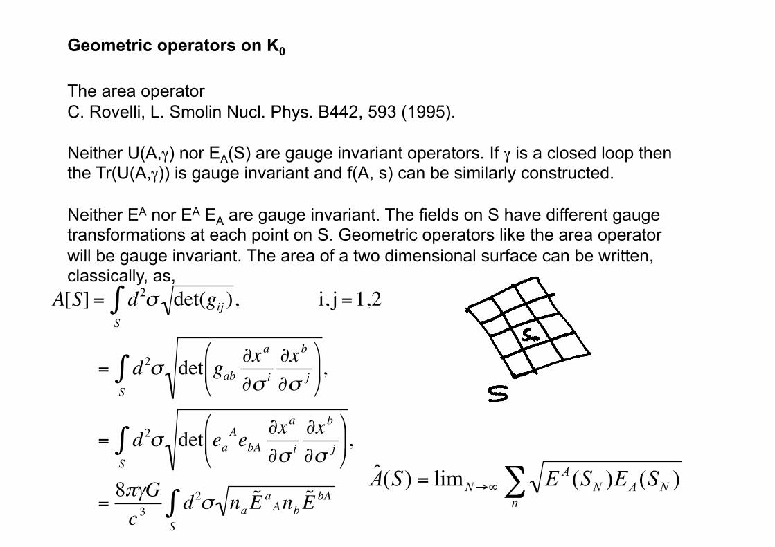
The area operator C. Rovelli, L. Smolin Nucl. Phys. B442, 593 (1995).

Neither U(A,γ) nor EA(S) are gauge invariant operators. If γ is a closed loop then the Tr(U(A,γ)) is gauge invariant and f(A, s) can be similarly constructed.

Neither EA nor EA EA are gauge invariant. The fields on S have different gauge transformations at each point on S. Geometric operators like the area operator will be gauge invariant. The area of a two dimensional surface can be written, classically, as,

€

A[S] = d2σS∫ det(gij ), i, j =1,2

= d2σS∫ det gab

∂xa

∂σ i∂xb

∂σ j

,

= d2σS∫ det ea

AebA∂xa

∂σ i∂xb

∂σ j

,

=8πγG

c 3 d2σS∫ na

˜ E a A nb˜ E bA

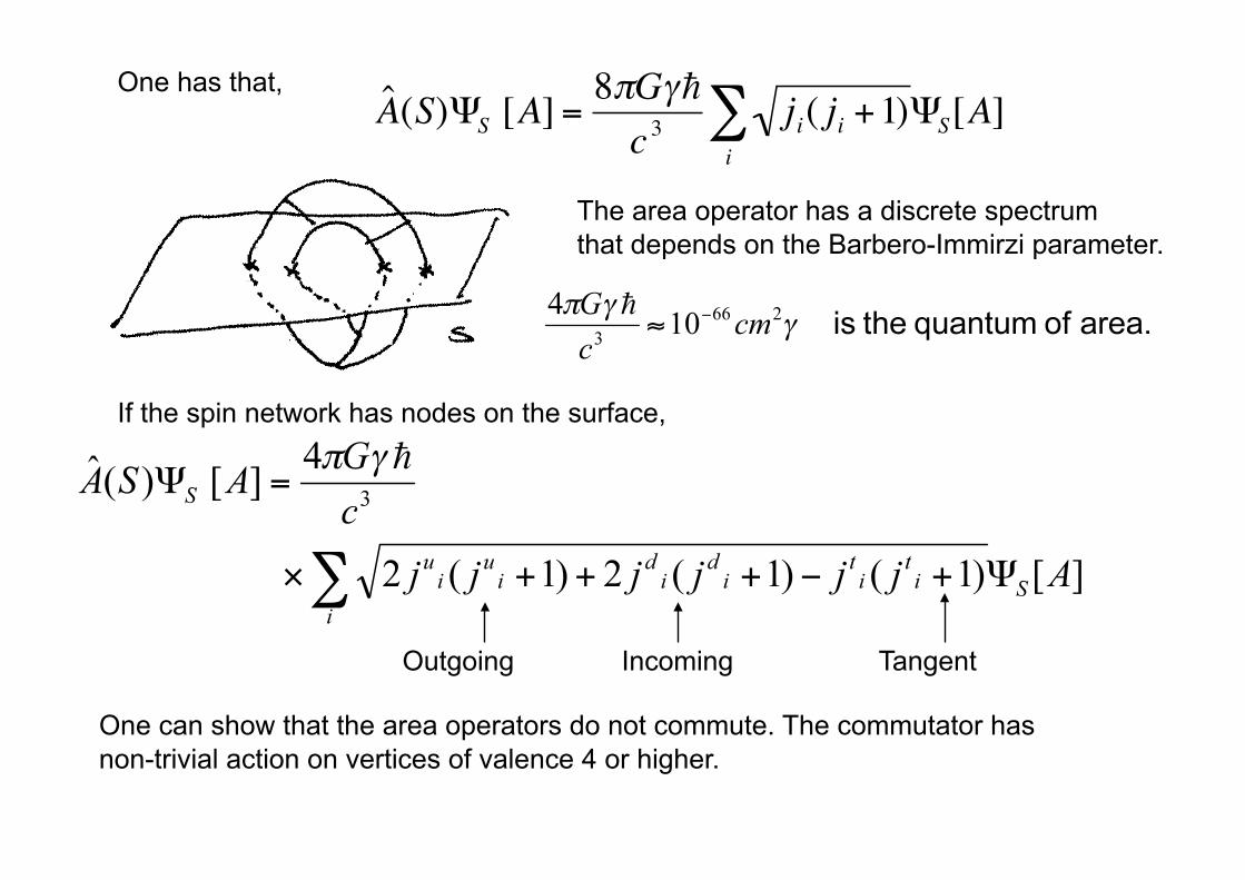
One has that,

€

ˆ A (S)ΨS [A] =8πGγ

c 3 ji( ji +1)i∑ ΨS[A]

The area operator has a discrete spectrum that depends on the Barbero-Immirzi parameter.

If the spin network has nodes on the surface,

Outgoing Incoming Tangent

One can show that the area operators do not commute. The commutator has non-trivial action on vertices of valence 4 or higher.

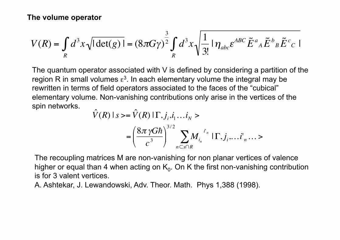
The volume operator

€

V (R) = d3x | det(g) |R∫ = (8πGγ)

32 d3x 1

3!|ηabcε

ABC ˜ E a A ˜ E b B ˜ E cC |R∫

The quantum operator associated with V is defined by considering a partition of the region R in small volumes ε3. In each elementary volume the integral may be rewritten in terms of field operators associated to the faces of the “cubical” elementary volume. Non-vanishing contributions only arise in the vertices of the spin networks.

€

ˆ V (R) | s >= ˆ V (R) |Γ, ji,i1…iN >

=8π γG

c 3

3 / 2

Minn⊂s∩R∑

i'n |Γ, ji,…i'n … >

The recoupling matrices M are non-vanishing for non planar vertices of valence higher or equal than 4 when acting on Κ0. On K the first non-vanishing contribution is for 3 valent vertices. A. Ashtekar, J. Lewandowski, Adv. Theor. Math. Phys 1,388 (1998).

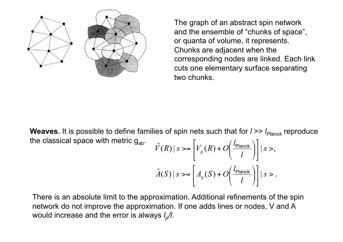
Fig 6.8 of Rovelli The graph of an abstract spin network and the ensemble of “chunks of space”, or quanta of volume, it represents. Chunks are adjacent when the corresponding nodes are linked. Each link cuts one elementary surface separating two chunks.

Weaves. It is possible to define families of spin nets such that for l >> lPlanck reproduce the classical space with metric gab.

There is an absolute limit to the approximation. Additional refinements of the spin network do not improve the approximation. If one adds lines or nodes, V and A would increase and the error is always lp/l.

The issue of the dynamics

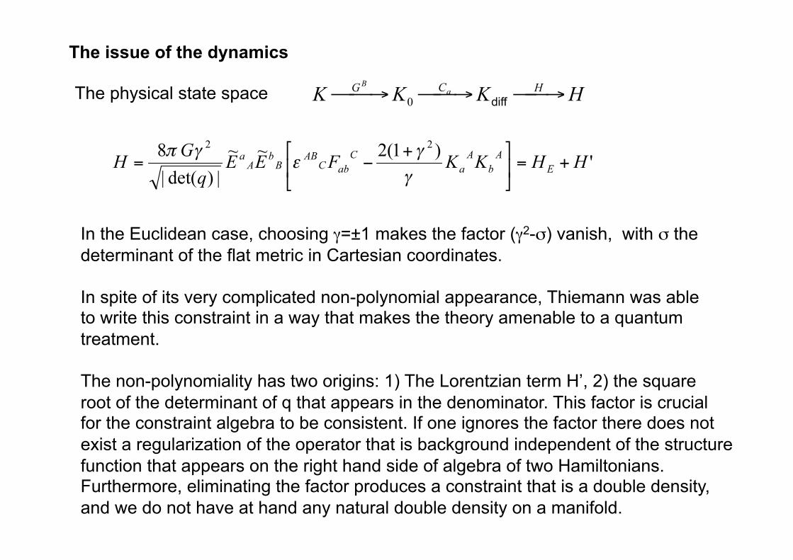
The physical state space

In the Euclidean case, choosing γ=±1 makes the factor (γ2-σ) vanish, with σ the determinant of the flat metric in Cartesian coordinates.

In spite of its very complicated non-polynomial appearance, Thiemann was able to write this constraint in a way that makes the theory amenable to a quantum treatment.

The non-polynomiality has two origins: 1) The Lorentzian term H’, 2) the square root of the determinant of q that appears in the denominator. This factor is crucial for the constraint algebra to be consistent. If one ignores the factor there does not exist a regularization of the operator that is background independent of the structure function that appears on the right hand side of algebra of two Hamiltonians. Furthermore, eliminating the factor produces a constraint that is a double density, and we do not have at hand any natural double density on a manifold.

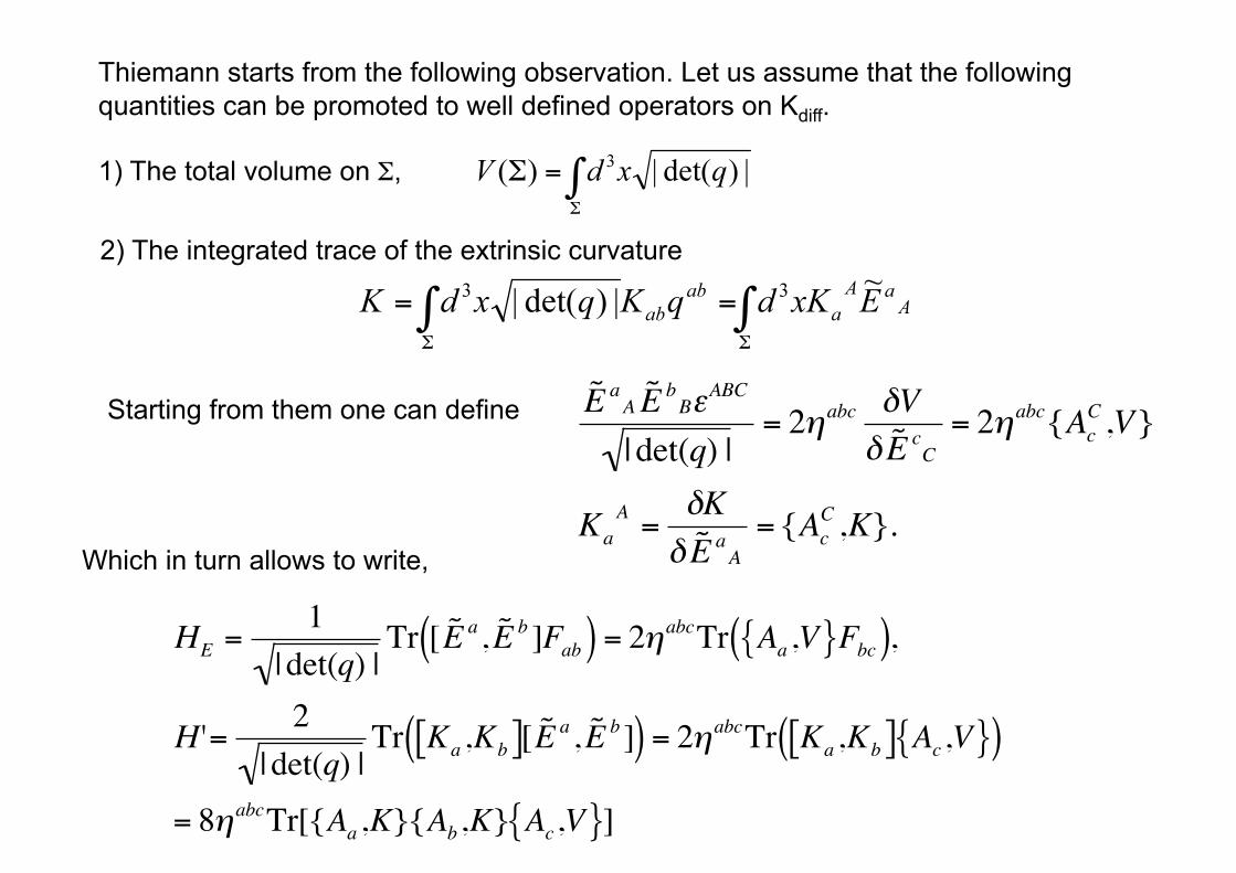
Thiemann starts from the following observation. Let us assume that the following quantities can be promoted to well defined operators on Kdiff.

1) The total volume on Σ,

2) The integrated trace of the extrinsic curvature

Starting from them one can define

€

˜ E a A ˜ E b BεABC

| det(q) |= 2ηabc δV

δ ˜ E cC= 2ηabc{Ac

C ,V}

KaA =

δKδ ˜ E a A

= {AcC ,K}.

Which in turn allows to write,

€

HE =1

| det(q) |Tr [ ˜ E a, ˜ E b ]Fab( ) = 2ηabcTr Aa ,V{ }Fbc( ),

H '= 2| det(q) |

Tr Ka ,Kb[ ][ ˜ E a , ˜ E b ]( ) = 2ηabcTr Ka ,Kb[ ] Ac,V{ }( )

= 8ηabcTr[{Aa ,K}{Ab,K} Ac,V{ }]

To promote those expressions to quantum operators, the Poisson brackets get promoted to commutators and as we shall see, all the quantities involved have well defined operators. We have already discussed the volume V. To quantize K one begins by noticing that,

€

K = −{V , d3x∫ HE},

where we have used that the integrated densitized trace of the extrinsic curvature is the “time derivative of the volume”.

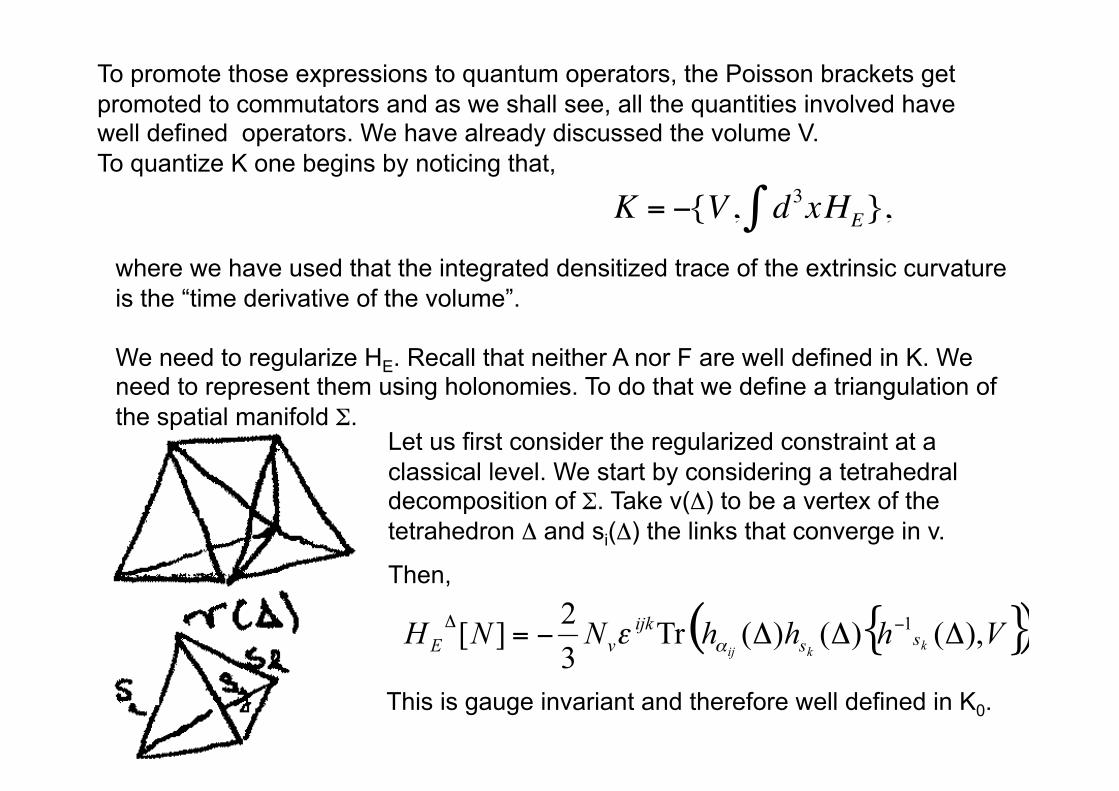
We need to regularize HE. Recall that neither A nor F are well defined in K. We need to represent them using holonomies. To do that we define a triangulation of the spatial manifold Σ.

Let us first consider the regularized constraint at a classical level. We start by considering a tetrahedral decomposition of Σ. Take v(Δ) to be a vertex of the tetrahedron Δ and si(Δ) the links that converge in v.

Then,

This is gauge invariant and therefore well defined in K0.

One can then write the Hamiltonian as a sum over the triangulation of the elementary contribution we just discussed,

€

HE = limΔ→0 H ΔE[N] =

Δ∈T∑ limΔ→0 NvH

vE

Δ∈T∑

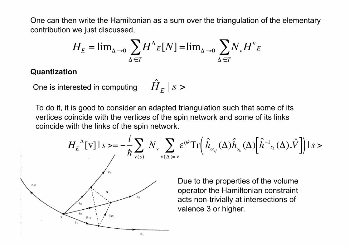
Quantization

One is interested in computing

To do it, it is good to consider an adapted triangulation such that some of its vertices coincide with the vertices of the spin network and some of its links coincide with the links of the spin network.

€

HEΔ[v] | s >= −

i v(s)∑ Nv

v(Δ )= v∑ ε ijkTr ˆ h α ij

(Δ) ˆ h sk(Δ) ˆ h −1

sk (Δ), ˆ V [ ]( ) | s >

Due to the properties of the volume operator the Hamiltonian constraint acts non-trivially at intersections of valence 3 or higher.

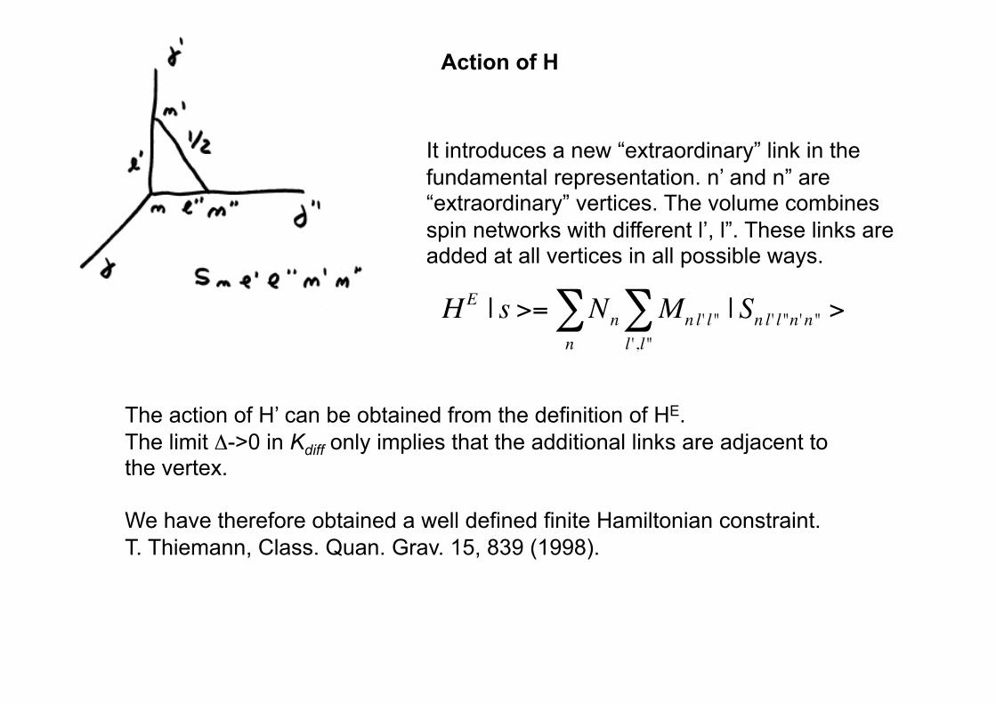
Action of H

It introduces a new “extraordinary” link in the fundamental representation. n’ and n” are “extraordinary” vertices. The volume combines spin networks with different l’, l”. These links are added at all vertices in all possible ways.

€

HE | s >= Nn Mnl ' l"l ',l"∑

n∑ | Snl ' l"n'n" >

The action of H’ can be obtained from the definition of HE. The limit Δ->0 in Kdiff only implies that the additional links are adjacent to the vertex.

We have therefore obtained a well defined finite Hamiltonian constraint. T. Thiemann, Class. Quan. Grav. 15, 839 (1998).

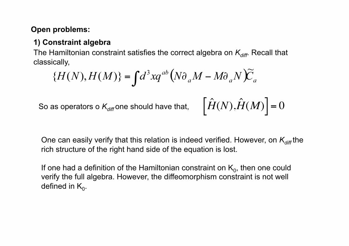
Open problems: 1) Constraint algebra The Hamiltonian constraint satisfies the correct algebra on Kdiff. Recall that classically,

So as operators o Kdiff one should have that,

€

ˆ H (N), ˆ H (M)[ ] = 0

One can easily verify that this relation is indeed verified. However, on Kdiff the rich structure of the right hand side of the equation is lost.

If one had a definition of the Hamiltonian constraint on K0, then one could verify the full algebra. However, the diffeomorphism constraint is not well defined in K0.

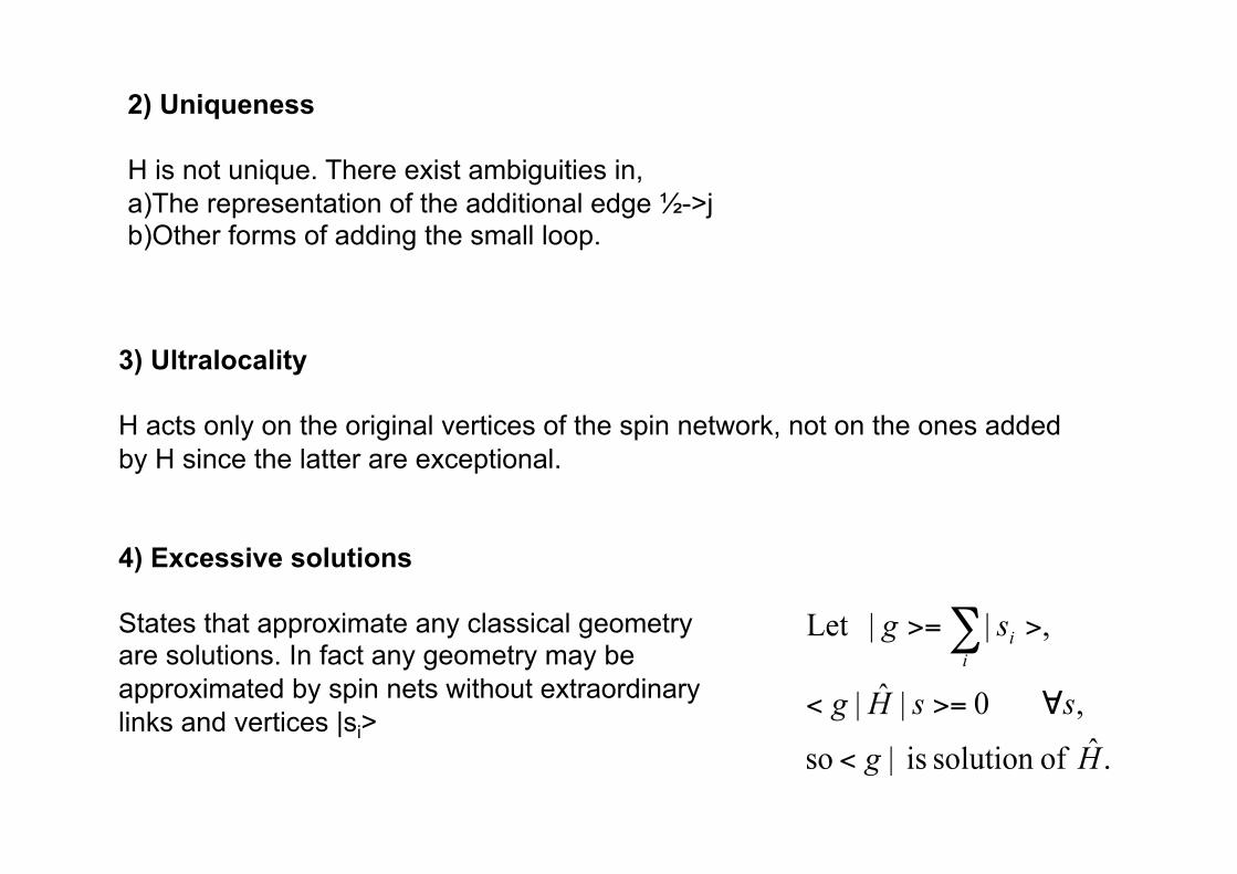
2) Uniqueness

H is not unique. There exist ambiguities in, a) The representation of the additional edge ½->j b) Other forms of adding the small loop.

3) Ultralocality

H acts only on the original vertices of the spin network, not on the ones added by H since the latter are exceptional.

4) Excessive solutions

States that approximate any classical geometry are solutions. In fact any geometry may be approximated by spin nets without extraordinary links and vertices |si>

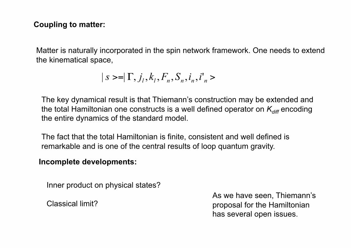
Coupling to matter:

Matter is naturally incorporated in the spin network framework. One needs to extend the kinematical space,

The key dynamical result is that Thiemann’s construction may be extended and the total Hamiltonian one constructs is a well defined operator on Kdiff encoding the entire dynamics of the standard model.

The fact that the total Hamiltonian is finite, consistent and well defined is remarkable and is one of the central results of loop quantum gravity.

Incomplete developments:

Inner product on physical states?

Classical limit? As we have seen, Thiemann’s proposal for the Hamiltonian has several open issues.

Other approaches to the dynamics of loop quantum gravity:

Spin foams: Reisenberger, Rovelli, Krasnov, Freidel, Pérez, many others.

Spin foam models for quantum gravity. Alejandro Pérez Jan 2003. 80pp. Class.Quant.Grav.20:R43,2003. e-Print: gr-qc/0301113

Master Constraint: Thiemann and collaborators.

The Phoenix project: Master constraint program for loop quantum gravity. Thomas Thiemann. Class.Quant.Grav.23:2211-2248,2006. gr-qc/0305080

Uniform discretizations: RG, Pullin.

Uniform discretizations: A New approach for the quantization of totally constrained systems. M. Campiglia, C Di Bartolo, R.G J.Pullin. Phys.Rev.D74:124012,2006. gr-qc/0610023

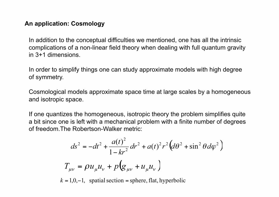
An application: Cosmology

In addition to the conceptual difficulties we mentioned, one has all the intrinsic complications of a non-linear field theory when dealing with full quantum gravity in 3+1 dimensions.

In order to simplify things one can study approximate models with high degree of symmetry.

Cosmological models approximate space time at large scales by a homogeneous and isotropic space.

If one quantizes the homogeneous, isotropic theory the problem simplifies quite a bit since one is left with a mechanical problem with a finite number of degrees of freedom.The Robertson-Walker metric:

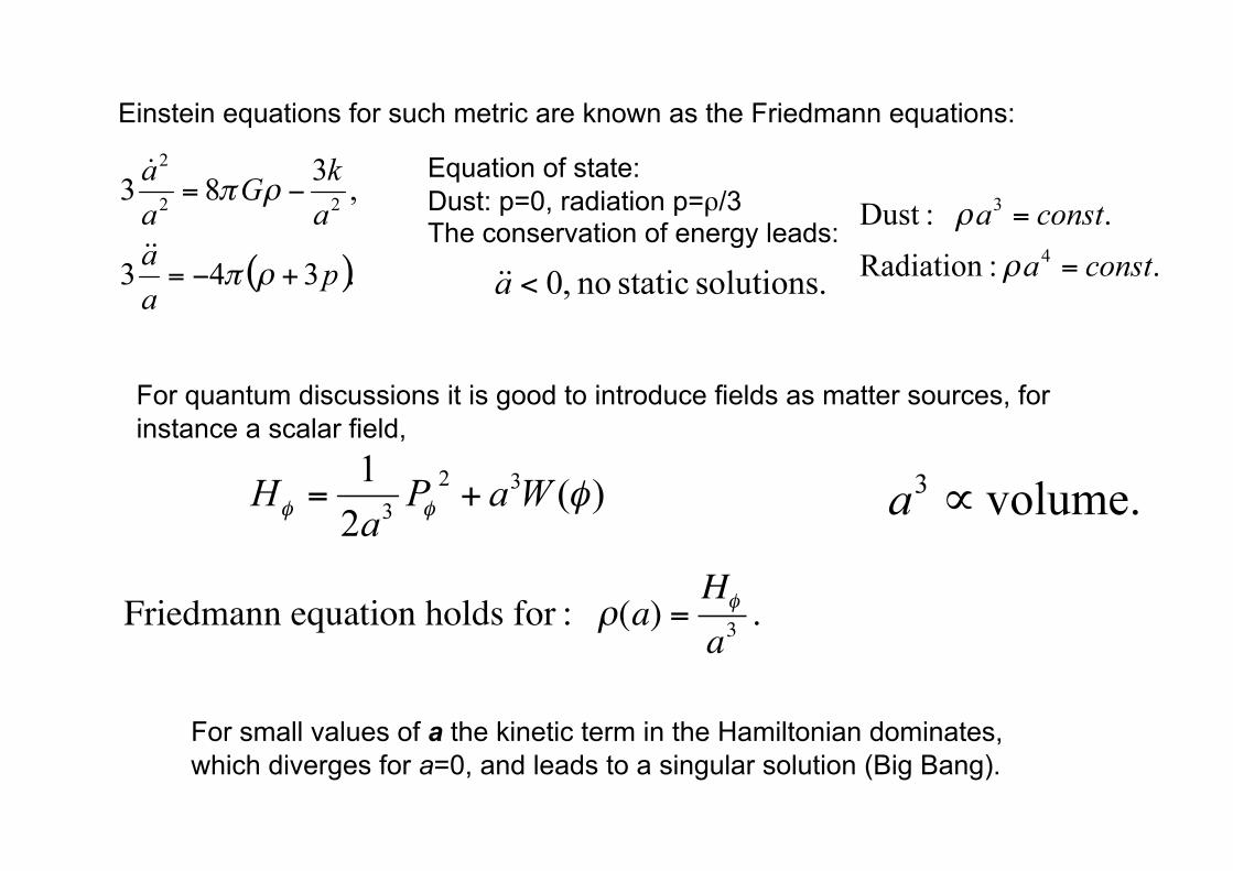
Einstein equations for such metric are known as the Friedmann equations:

Equation of state: Dust: p=0, radiation p=ρ/3 The conservation of energy leads:

For quantum discussions it is good to introduce fields as matter sources, for instance a scalar field,

€

Friedmann equation holds for : ρ(a) =Hφ

a3 .

For small values of a the kinetic term in the Hamiltonian dominates, which diverges for a=0, and leads to a singular solution (Big Bang).

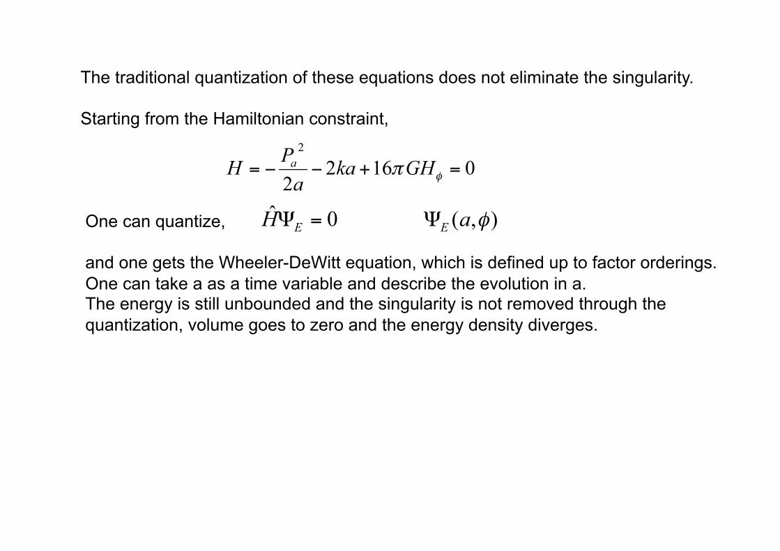
The traditional quantization of these equations does not eliminate the singularity.

Starting from the Hamiltonian constraint,

One can quantize,

and one gets the Wheeler-DeWitt equation, which is defined up to factor orderings. One can take a as a time variable and describe the evolution in a. The energy is still unbounded and the singularity is not removed through the quantization, volume goes to zero and the energy density diverges.

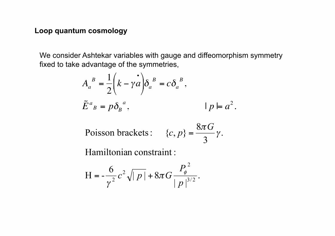
Loop quantum cosmology

We consider Ashtekar variables with gauge and diffeomorphism symmetry fixed to take advantage of the symmetries,

€

AaB =

12

k − γa•

δa

B = cδaB ,

˜ E a B = pδBa , | p |= a2 .

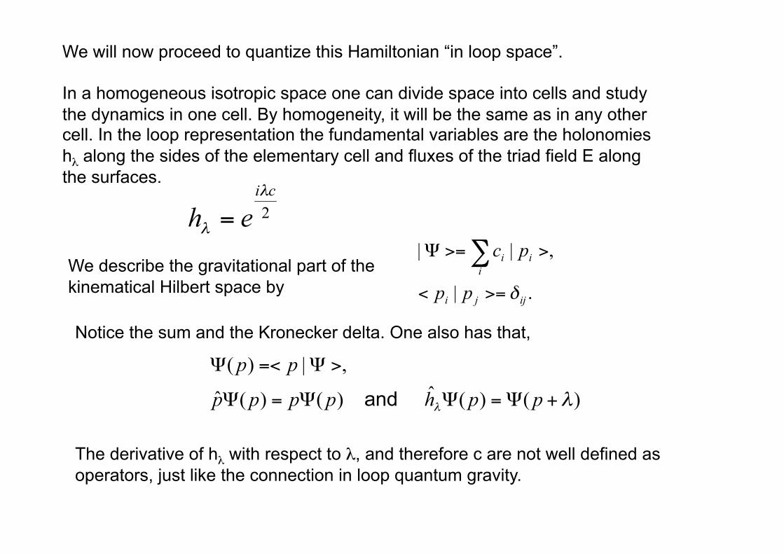
We will now proceed to quantize this Hamiltonian “in loop space”.

In a homogeneous isotropic space one can divide space into cells and study the dynamics in one cell. By homogeneity, it will be the same as in any other cell. In the loop representation the fundamental variables are the holonomies hλ along the sides of the elementary cell and fluxes of the triad field E along the surfaces.

We describe the gravitational part of the kinematical Hilbert space by

Notice the sum and the Kronecker delta. One also has that,

The derivative of hλ with respect to λ, and therefore c are not well defined as operators, just like the connection in loop quantum gravity.

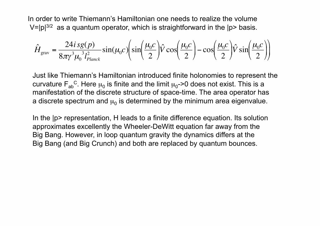
In order to write Thiemann’s Hamiltonian one needs to realize the volume V=|p|3/2 as a quantum operator, which is straightforward in the |p> basis.

€

ˆ H grav =24i sg(p)

8πγ 3µ03lPlanck

2 sin(µ0c) sin µ0c2

ˆ V cos µ0c

2

− cos µ0c

2

ˆ V sin µ0c

2

Just like Thiemann’s Hamiltonian introduced finite holonomies to represent the curvature Fab

C. Here µ0 is finite and the limit µ0->0 does not exist. This is a manifestation of the discrete structure of space-time. The area operator has a discrete spectrum and µ0 is determined by the minimum area eigenvalue.

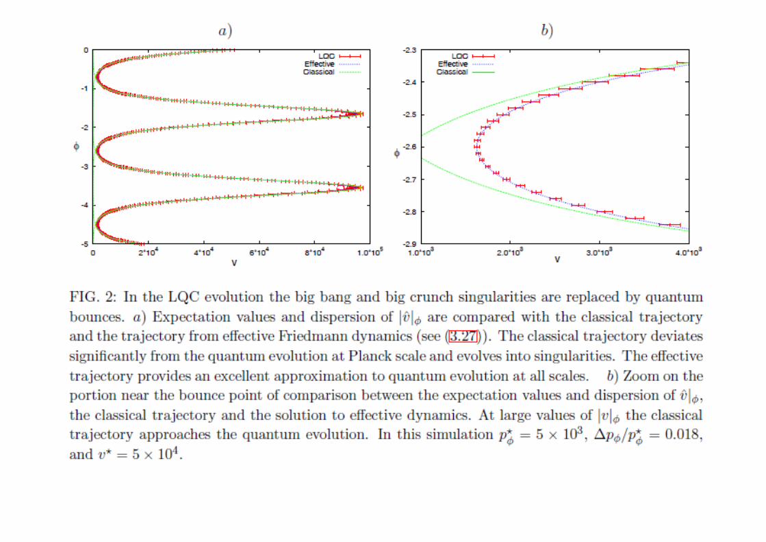
In the |p> representation, H leads to a finite difference equation. Its solution approximates excellently the Wheeler-DeWitt equation far away from the Big Bang. However, in loop quantum gravity the dynamics differs at the Big Bang (and Big Crunch) and both are replaced by quantum bounces.

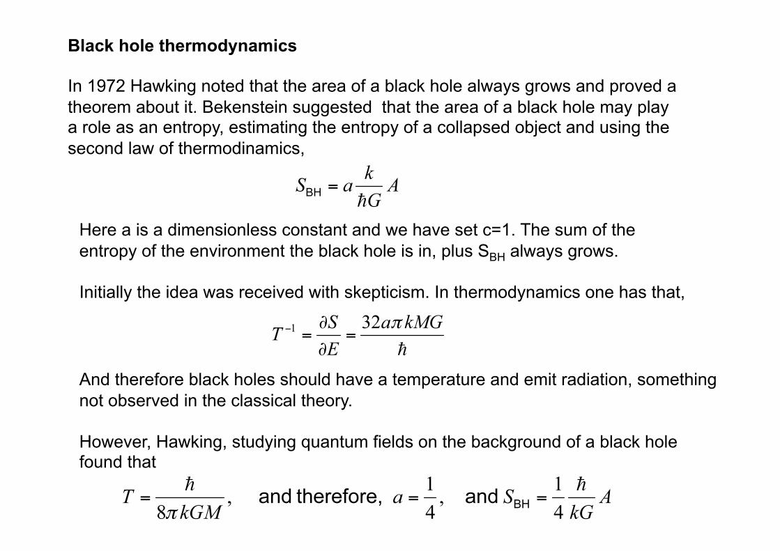
Black hole thermodynamics

In 1972 Hawking noted that the area of a black hole always grows and proved a theorem about it. Bekenstein suggested that the area of a black hole may play a role as an entropy, estimating the entropy of a collapsed object and using the second law of thermodinamics,

Here a is a dimensionless constant and we have set c=1. The sum of the entropy of the environment the black hole is in, plus SBH always grows.

Initially the idea was received with skepticism. In thermodynamics one has that,

And therefore black holes should have a temperature and emit radiation, something not observed in the classical theory.

However, Hawking, studying quantum fields on the background of a black hole found that

This opens several new questions:

Do this results hold in quantum gravity?

What is the statistical origin of S?

The presence of ħ confirms that quantum gravity must play a role.

We will see that loop quantum gravity leads to this result and does so for black holes of different type.

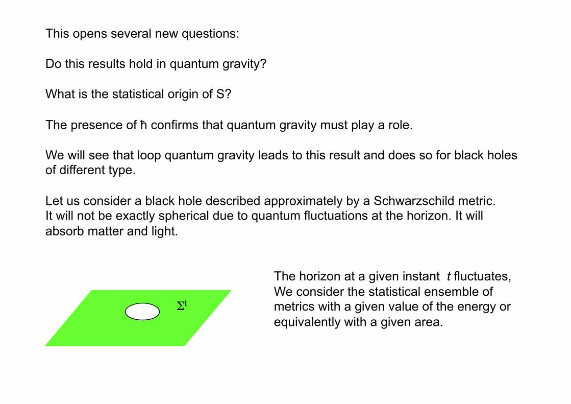
Let us consider a black hole described approximately by a Schwarzschild metric. It will not be exactly spherical due to quantum fluctuations at the horizon. It will absorb matter and light.

Σt

The horizon at a given instant t fluctuates, We consider the statistical ensemble of metrics with a given value of the energy or equivalently with a given area.

All the information we have about a black hole is on its horizon, we can cannot get information about what happens behind the horizon through the fluctuations of the latter.

Other types of systems trapped in a box S, one can know what happens in the interior and therefore increase the information and lower the entropy. This does not occur in black holes.

We must therefore determine the ensemble of microstates gt. In statistical mechanics a microcanonical ensemble has states of a given energy E. In this case we are interested in the state of area A, proportional to M2. If there are N(A) states with area A,

In order to determine N(A) we observe that classically such number is infinite but quantum mechanically it will correspond to the number of orthogonal states with area A.

The number of different quantum configurations in the spin net basis will correspond to the number of possible spin nets with area A at the horizon.

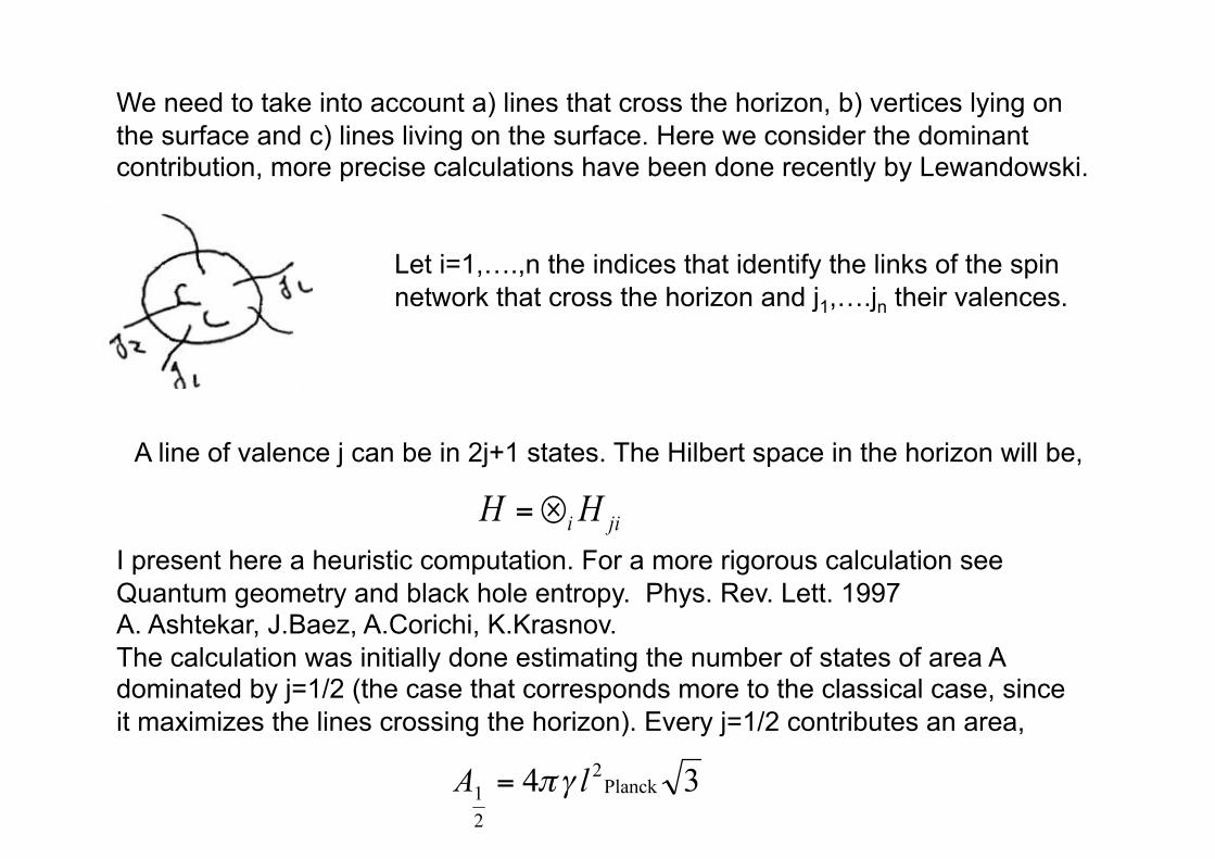
We need to take into account a) lines that cross the horizon, b) vertices lying on the surface and c) lines living on the surface. Here we consider the dominant contribution, more precise calculations have been done recently by Lewandowski.

Let i=1,….,n the indices that identify the links of the spin network that cross the horizon and j1,….jn their valences.

A line of valence j can be in 2j+1 states. The Hilbert space in the horizon will be,

I present here a heuristic computation. For a more rigorous calculation see Quantum geometry and black hole entropy. Phys. Rev. Lett. 1997 A. Ashtekar, J.Baez, A.Corichi, K.Krasnov. The calculation was initially done estimating the number of states of area A dominated by j=1/2 (the case that corresponds more to the classical case, since it maximizes the lines crossing the horizon). Every j=1/2 contributes an area,

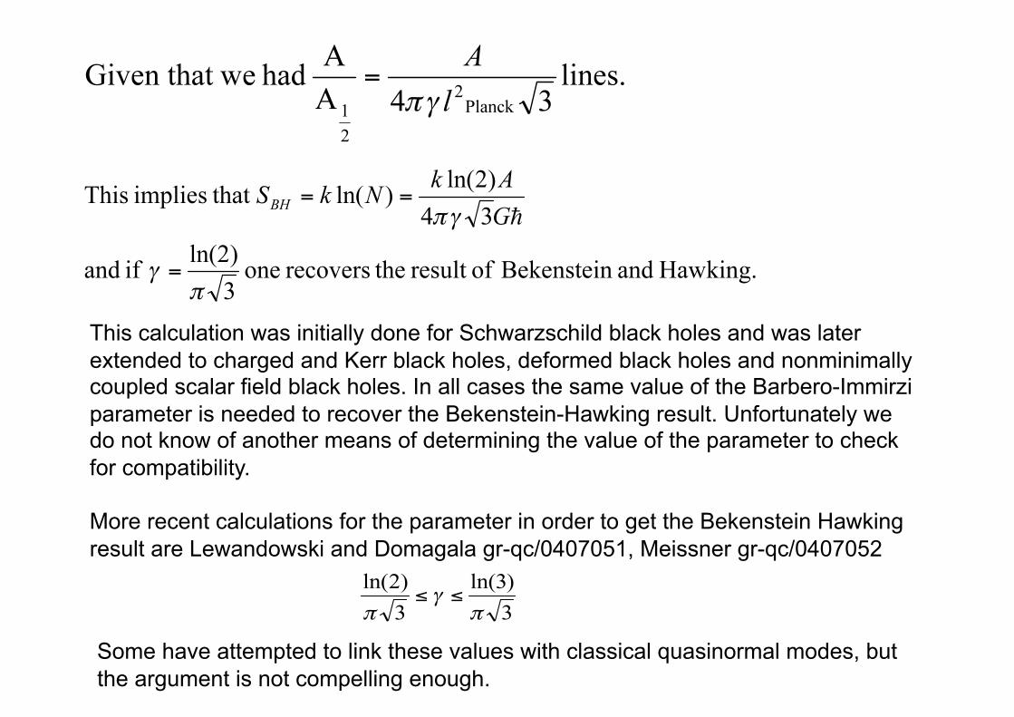
This calculation was initially done for Schwarzschild black holes and was later extended to charged and Kerr black holes, deformed black holes and nonminimally coupled scalar field black holes. In all cases the same value of the Barbero-Immirzi parameter is needed to recover the Bekenstein-Hawking result. Unfortunately we do not know of another means of determining the value of the parameter to check for compatibility.

More recent calculations for the parameter in order to get the Bekenstein Hawking result are Lewandowski and Domagala gr-qc/0407051, Meissner gr-qc/0407052

Some have attempted to link these values with classical quasinormal modes, but the argument is not compelling enough.

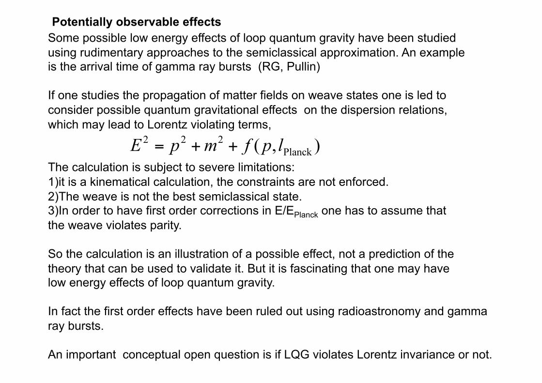
Potentially observable effects Some possible low energy effects of loop quantum gravity have been studied using rudimentary approaches to the semiclassical approximation. An example is the arrival time of gamma ray bursts (RG, Pullin)

If one studies the propagation of matter fields on weave states one is led to consider possible quantum gravitational effects on the dispersion relations, which may lead to Lorentz violating terms,

The calculation is subject to severe limitations: 1) it is a kinematical calculation, the constraints are not enforced. 2) The weave is not the best semiclassical state. 3) In order to have first order corrections in E/EPlanck one has to assume that the weave violates parity.

So the calculation is an illustration of a possible effect, not a prediction of the theory that can be used to validate it. But it is fascinating that one may have low energy effects of loop quantum gravity.

In fact the first order effects have been ruled out using radioastronomy and gamma ray bursts.

An important conceptual open question is if LQG violates Lorentz invariance or not.

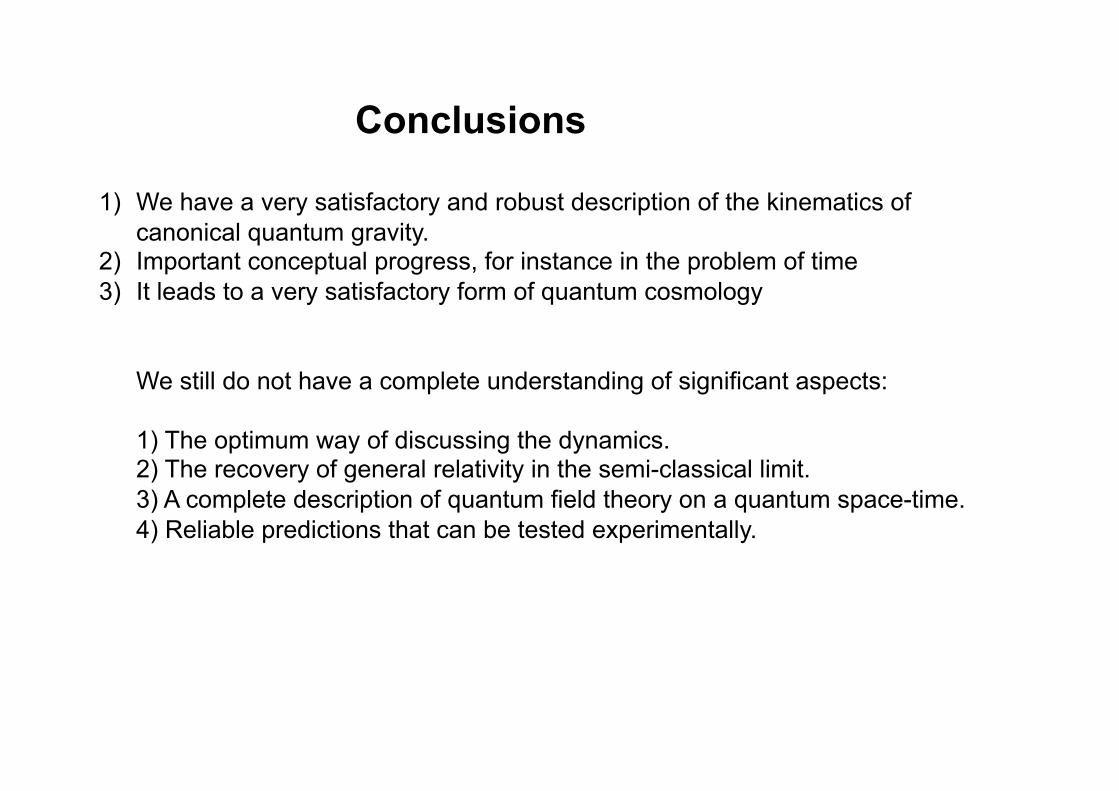
Conclusions

1)  We have a very satisfactory and robust description of the kinematics of canonical quantum gravity.

2)  Important conceptual progress, for instance in the problem of time 3)  It leads to a very satisfactory form of quantum cosmology

We still do not have a complete understanding of significant aspects:

1) The optimum way of discussing the dynamics. 2) The recovery of general relativity in the semi-classical limit. 3) A complete description of quantum field theory on a quantum space-time. 4) Reliable predictions that can be tested experimentally.