Lectures on Landau Theory of Phase Transitions

Lectures on Landau Theoryof Phase Transitions

Department of Physics, Georgetown University

Peter D Olmsted

July 9, 2015

Contents

1 Goals of these Lectures 1

2 Phase Transitions 2

2.1 Examples . . . . . . . . . . . . . . . . . . . . . . . . . . . . . . . . . . . . . 2

2.2 Statistical Mechanics and Phase Transitions . . . . . . . . . . . . . . . . . . 3

3 Landau Theory: Fundamentals 5

3.1 The Recipe . . . . . . . . . . . . . . . . . . . . . . . . . . . . . . . . . . . . 5

3.2 Relation to Statistical Mechanics . . . . . . . . . . . . . . . . . . . . . . . . 6

4 Examples 7

4.1 Ising Magnet . . . . . . . . . . . . . . . . . . . . . . . . . . . . . . . . . . . 8

4.2 Heisenberg Ferromagnet . . . . . . . . . . . . . . . . . . . . . . . . . . . . . 9

4.3 Nematic Liquid Crystals . . . . . . . . . . . . . . . . . . . . . . . . . . . . . 10

4.4 Crystal Systems . . . . . . . . . . . . . . . . . . . . . . . . . . . . . . . . . . 14

4.4.1 Lamellar Systems . . . . . . . . . . . . . . . . . . . . . . . . . . . . . 14

4.4.2 Two and Three Dimensional Crystals . . . . . . . . . . . . . . . . . . 15

i

5 Smectic Liquid Crystals 18

5.1 Mean Field Theory of the Nematic-Smectic–A transition . . . . . . . . . . . 18

5.2 Free Energy and Superconducting Analogy . . . . . . . . . . . . . . . . . . . 19

5.3 Fluctuations and the Halperin-Lubensky-Ma Effect. . . . . . . . . . . . . . . 21

5.4 Layered liquids and the Brazovskii effect . . . . . . . . . . . . . . . . . . . . 22

Distributed under Creative Commons License Attribution 4.0 International.c© Peter D. Olmsted (2015).

ii

1. Goals of these Lectures Lectures on Landau Theory

1 Goals of these Lectures

Phase transitions are ubiquitous in nature. Examples include a magnets, liquid crystals,superconductors, crystals, amorphous equilibrium solids, and liquid condensation. Thesetransitions occur between equilibrium states as functions of temperature, pressure, magneticfield, etc.; and define the nature of the matter we deal with on a day to day basis. Under-standing how to predict and describe both the existence of these transitions, as well as theircharacter and consequences for everyday phenemena, is one of the more important roles ofstatistical and condensed matter physics.

In this brief set of Lectures I propose to outline one of the basic theoretical tools fordescribing phase transitions, the Landau Theory of Phase Transitions. This was de-veloped by Landau in the 1940’s, originally to describe superconductivity. The procedure isgeneral, and is one of the most useful tools in condensed matter physics. Not only can we useLandau Theory to describe and understand the nature of phase transitions among ordered(and disordered) states, but we can use it as a starting point for understanding the behaviorof ordered states. These lectures are designed to establish the following broad brush strokes:

1. Very few phase transitions can be calculated exactly: nonetheless, there is still muchthat can be understood without having to solve the entire problem. These kinds ofquestions (order of phase transitions, hydrodynamics and elasticity, fluctuations) arethe domain of Landau theory.

2. I will present (some of) the problems of phase transitions, and introduce Landau Theoryas a way of understanding the behavior (but not the existence) of phase transitions.

3. We will explore, through examples, the profound implications of symmetry for thenature of ordered states and their associated transitions.

4. We will see how to use the nature of the order parameter to understand deformationsin a broken symmetry state: this often goes by the name of generalized elasticity,and incorporates elasticity of solids, Frank elasticity in nematic liquid crystals, thedeformation energy of smectic liquid crystals and membrane systems, sound waves influids, etc.

5. Landau theory is a mean field theory, in the sense that the system is assumed to beadequately described by a single macroscopic state.

6. We will use Landau free energy functionals to calculate observable quantities such asstructure factors; identify the breakdown of Landau theory due to fluctuations.

7. We will examine some interesting paradigms whereby the qualitative nature of phasetransitions, such as the order of the phase transition, is altered by fluctuation effectsand the coupling of different degrees of freedom.

Along the way we will learn how to follow our noses and construct proper free energyfunctionals on symmetry grounds; pick up some calculational tools; and examine some fun-damental ideas in statistical mechanics.

1 c© Peter D. Olmsted, 2015.

2. Phase Transitions Lectures on Landau Theory

2 Phase Transitions

A phase transition occurs when the equilibrium state of a system changes qualitatively asa function of externally imposed constraints. These constraints could be temperature, pres-sure, magnetic field, concentration, degree of crosslinking, or any number of other physicalquantities. In the following I only consider a transition as a function of temperature, butnote that the idea is, of course, more general than that (physicists strive to be as general aspossible!). In any of these transitions there is some quantity that can be observed to changequalitatively as a function of temperature. In many cases more than one quantity can beobserved, but it is quite obvious that something is happening. This quantity will be takenlater to be the order parameter of the phase transition.

2.1 Examples

1. Crystals: In a transition to a crystalline solid a disordered liquid with non apparentstructure undergoes a transition to a structure with long range periodic order, usuallyin three dimensions. This is most easily parametrized by the mass density, ρ(r):

ρ(r) = ρ+∑

q∈G

[ρ(q)e−iq·r + c.c

], (1)

where ρ is the mean density and {G} is theset of reciprocal lattice vectors that char-acterize the crystal structure. The Fouriermodes refer to density modulations withwavenumber q = 2π/λ, with wavelengthλ. The complex conjugate is added to re-tain a real number for the mass density.Upon cooling a liquid into a crystal theobject that distinguishes the crystal fromthe liquid is the set of wavevectors {ρ(G)},which appear as Bragg peaks in a scat-tering experiment. Usually these Fouriermodes grow discontinuously from zero, inwhat is called a first order phase tran-

sition:

Tc

Temperature

orde

r pa

ram

eter

First Order Phase Transition(Nematic LC, 2D/3D crystals, etc)

2. Nematic Liquid Crystals: The isotropic-nematic transition occurs in melts (orsolutions) of rigid rod-like molecules. At high temperatures (or dilute concentrations)the rods are isotropically distributed, and upon cooling an orientational interactionwhich is a combination of enthalpic and excluded volume effects encourages the rodsto spontaneously align along a particular direction, denoted the director, n. A scalarmeasure of the order is the anisotropy of the distribution of rods,

〈P2(cos θ)〉 = 〈cos2 θ − 13〉, (2)

where the average 〈·〉 is taken over the equilibrium distribution for all rods in thesystem, and θ is the angle with respect to some fixed direction. Like 2D crystallization,


2.2 Statistical Mechanics and Phase Transitions Lectures on Landau Theory

the isotropic-nematic is a first order transition, with a discontinuity in 〈P2(cos θ)〉 at thetransition temperature TIN . Since “up” and “down” are the same for such a system (inliquid crystals the rodlike molecules are typically symmetric under reflection throughthe long axis), the order parameter is symmetric under cos θ → − cos θ.

3. Magnets: In a ferromagnet an assemblyof magnetic spins undergoes a spontaneoustransition from a disordered phase with nonet magnetization to a phase with a non-zero magnetization. The order parameteris thus the magnetization,

M =1

N

∑

i

〈Si〉, (3)

where the average is an equilibrium aver-age over all spins Si in the system. Un-like the nematic liquid crystal, the ferro-magnetic phase transition is a continuousphase transition, in which the magne-tization grows smoothly from zero below

a critical temperature Tc (often called theCurie Temperature, after its discoverer).

Tc

Temperature

orde

r pa

ram

eter

Continuous Phase Transition (Magnet, superconductor, 1D crystal, ...)

4. One Dimensional (layered) Crystals: In a one dimensional crystal, or a layeredsystem, a one-dimensional modulation develops spontaneously below the critical tem-perature. Examples include block-copolymers, which can phase separate into layers ofA and B material, to relieve chemical incompatibility but maintain the connectivityconstraint; helical magnets which develop a pitch as the spin twists; cholesteric phaseswhich develop a twisted nematic conformation; and smectic phases in thermotropicliquid crystals and lyotropic surfactant solutions. In this case the order parameter isthe Fourier mode of the relevant degree of freedom:

ψ(r) = ψ + ψ(q)e−iq·r + c.c. (4)

This transition is predicted by Landau (mean field) theory to be continuous, but it isbelieved to be first order in physical situations, due to fluctuation effects. Hopefullywe will get this far!

5. Phase Separation: Finally, one of the most common phase transitions from everyday life is phase separation, which makes it necessary to shake the salad dressing. Inthis case the order parameter is the deviation of the local composition from the meanvalue. Usually this is a first order phase transition, but if the concentration is justright the system can be taken through a critical point, or continuous phase transition.This system is equivalent to liquid-liquid or liquid-gas phase separation, in which casethe order parameter is a density difference instead of a composition difference.

2.2 Statistical Mechanics and Phase Transitions

One of the uses of statistical mechanics (aside from helping us to understand nature) is tocalculate fundamental properties of matter, including phase transitions. In principle, this


2.2 Statistical Mechanics and Phase Transitions Lectures on Landau Theory

is a remarkably simple task, thanks to Boltzmann. All of the statistical information of asystem is encoded in the Partition Function, Z:

Z =∑

µ

e−H[µ]/kBT , (5)

where µ refers to all the microstates of the system (e.g. all possible configurations spins ina magnet) and H[µ] is the Hamiltonian (energy). Boltzmann proved that the (Helmholtz)free energy is given by

F = −kBT lnZ. (6)

If we can calculate the free energy F we can then calculate all desired thermodynamicquantities by appropriate derivatives.∗ Unfortunately, the free energy can only be evaluatedfor a few systems, notably the Ising Model (spins which can point up or down, and interactwith each other by a very simple interaction, H = −J

∑ij SiSj). More often than not we

are faced with an impossibly difficult calculation.

In the case of phase transitions, perhaps we can get away with a less rigorous calculation.A clue is the very nature of a phase transition: at a phase transition a system undergoes aqualitative change, and develops some order where there was none before. Hence the systemdoes not vary smoothly as a function of (for example) temperature. This means that thefree energy F (T ) is, mathematically, a non-analytic function of temperature. This is offundamental importance in the theory of phase transitions, and forms the starting point ofrigorous studies. A non-analytic function is one for which some derivatives are undefinedat certain points, or singularities. Phase transitions are points (in the parameter space offield variables such as temperature, pressure, magnetic field) or sets of points which aresingularities in the free energy. The free energy, and hence the behavior of a thermodynamic

system, behaves non-smoothly as it is taken through a phase transition.

It’s interesting to try and understand how to get non-analytic behavior out of a sum ofexponentials, each of which is separately analytic at any finite temperature:

F = −kBT ln

[∑

µ

e−H[µ]/kBT

]. (9)

The existence of singularities in F is a direct result of the thermodynamic limit, that is, thepresence of an essentially infinite number of degrees of freedom in a thermodynamic system.Possible singularities we can imagine in F are discontinuities in the first derivative, ∂F/∂T ,

∗For example, the magnetization can be determined by

M = − ∂F

∂h

∣∣∣∣h=0

, (7)

where an additional symmetry-breaking field has been added to the system Hamiltonian. For any system,it’s only a matter of cleverness to determine the extra field to add to “extract” the desired order parameterby a suitable derivative. In this case the field enters as

H[S] → H[S]− h∑

i

Si. (8)


3. Landau Theory: Fundamentals Lectures on Landau Theory

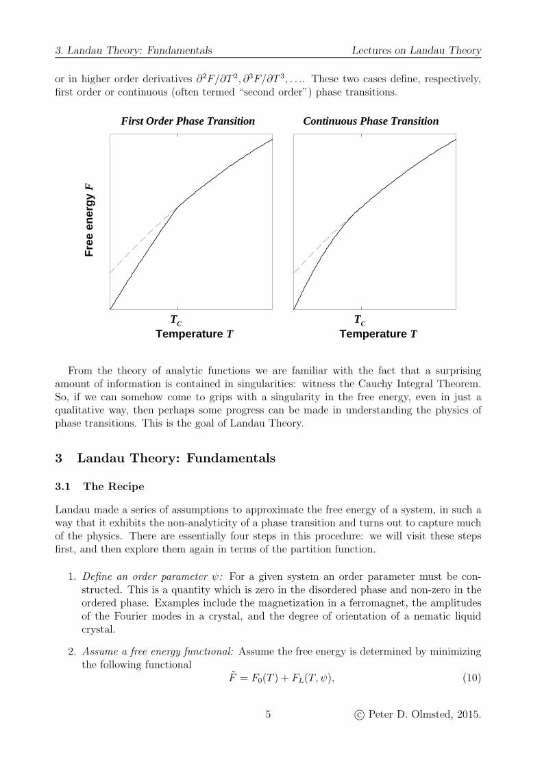
or in higher order derivatives ∂2F/∂T 2, ∂3F/∂T 3, . . .. These two cases define, respectively,first order or continuous (often termed “second order”) phase transitions.

TC

Temperature T

Fre

e en

erg

y F

First Order Phase Transition

TC

Temperature T

Continuous Phase Transition

From the theory of analytic functions we are familiar with the fact that a surprisingamount of information is contained in singularities: witness the Cauchy Integral Theorem.So, if we can somehow come to grips with a singularity in the free energy, even in just aqualitative way, then perhaps some progress can be made in understanding the physics ofphase transitions. This is the goal of Landau Theory.

3 Landau Theory: Fundamentals

3.1 The Recipe

Landau made a series of assumptions to approximate the free energy of a system, in such away that it exhibits the non-analyticity of a phase transition and turns out to capture muchof the physics. There are essentially four steps in this procedure: we will visit these stepsfirst, and then explore them again in terms of the partition function.

1. Define an order parameter ψ: For a given system an order parameter must be con-structed. This is a quantity which is zero in the disordered phase and non-zero in theordered phase. Examples include the magnetization in a ferromagnet, the amplitudesof the Fourier modes in a crystal, and the degree of orientation of a nematic liquidcrystal.

2. Assume a free energy functional: Assume the free energy is determined by minimizingthe following functional

F = F0(T ) + FL(T, ψ), (10)


3.2 Relation to Statistical Mechanics Lectures on Landau Theory

where F0 is an analytic (smooth) function of temperature, and FL(T, ψ) contains allthe information about dependence on the order parameter ψ.

3. Construction of FL(ψ): The Landau Functional is assumed to be an analytic (typicallypolynomial expansion) function of ψ that obeys all possible symmetries associated withψ; this typically includes translational and rotational invariance, and other “internal”degrees of dicatated by the nature of the order parameter. This is the most importantpart of the theory, wherein most of the physics lies.

4. Temperature Dependence: It is assumed that all the non-trivial temperature depen-dence resides in the lowest order term in the expansion of FL(T, ψ), typically of theform

FL[T, ψ] =

∫dV

[12a0(T − T∗)ψ

2 + . . .]

(11)

Since FL is constructed as an expansion, there will be other unknown constants. Ina physical system these constants have temperature dependence, but if these depen-dences are smooth then they have negligible effect near the phase transition. This isrigorous for a continuous phase transition, and an approximation for a first order phasetransition.

Upon constructing the Landau functional, and minimizing it over ψ as a function of tem-perature, the nature of the phase transition may be determined. The system at this level isspecified as having a uniform, or mean, state; hence Landau theory is really a mean field the-ory. However, the resulting approximate free energy is a natural starting point for examiningfluctuation effects.

3.2 Relation to Statistical Mechanics

To understand what’s going on, let’s reexamine statistical mechanics. The free energy isgiven by

e−F/kBT =∑

µ

e−H[µ]/kBT . (12)

Landau’s assumption is that we can replace the entire partition function by the following,

e−F/kBT ≃ e−F0/kBT

∫Dψ e−FL[T,ψ]/kBT , (13)

where the integral∫Dψ is a functional integral over all degrees of freedom associated with

ψ, instead of an integral over all microstates. For example, if ψ is the mean magnetization,a given value for the magnetization can be determined by many different microstates. It isassumed that all of this information is contained in FL. This is a non-trivial assumption whichcan nonetheless be proven for certain systems. The conversion of the degree of freedom fromµ to ψ is known as coarse-graining, and is at the heart of the relationship between statisticalmechanics and thermodynamics. The next step is to minimize FL[T, ψ], giving:

e−F/kBT ≃ e−F0/kBT e−min{ψ} FL[T,ψ]/kBT . (14)

This is tantamount to performing a saddle point approximation to the function integral inEq. (13).


4. Examples Lectures on Landau Theory

Here’s a more formal rationalization:

e−F/kBT =∑

µ

e−H[µ]/kBT exact Partition Function (15a)

=∑

µ

∫Dψ δ[ψ − 〈µ〉]e−H[µ]/kBT introduce ψ as an average over µ (15b)

=

∫Dψ

∑

µ

δ[ψ − 〈µ〉]e−H[µ]/kBT interchange limits (15c)

≃∫

Dψ g(ψ)e−H[ψ]/kBT

• g(ψ) represents the degeneracy ofψ (number of microstates)

• H[µ] → H[ψ] is generally incor-rect, but illustrates the idea.

(15d)

=

∫Dψ e−[H[ψ]−kBT ln g(ψ)]/kBT (15e)

⇒ F ≃ minψ

[H[ψ]− kBT ln g(ψ)] . saddle point approximation (15f)

Now, the free energy of a system is given by

F = E − TS. (16)

Hence ln g(ψ) is essentially the entropy of the system. To rationalize the assumed form ofthe temperature dependence of FL[T, ψ], we write:

F

Volume≃ E0 −E∗ψ

2

︸︷︷︸attraction

+ . . .− T [S0 −aψ2 + . . .︸︷︷︸reduction due to ordering

] (17a)

= F0 + a(T − E∗

a)ψ2 + . . . (17b)

We assume there is some “attraction” neccessary to induce order in the system, but this oc-curs at the expense of reducing the entropy; this, in principle, is contained in the degeneracyg(ψ). The competition of these effects leads to a phase transition.

In a physical system, the steps between Eq. (15c) and Eq. (15d) is exceedingly difficult,since the relationship between ψ and µ is often not simple, and usually a different functionalform than the appearance of µ in the original HamiltonianH[µ]. Hence this procedure shouldbe considered a cartoon; in reality, H[ψ] and g[ψ] are inextricably and inseparably boundinto FL[ψ].

†

4 Examples

To make this discussion concrete and useful we must examine some physical systems. Wewill do this in order of complexity, and gradually introduce important concepts and gener-alizations as they appear.

†In the case of polymer blends, where the Hamiltonian is given by H = −∑

α,β φα Vαβ φβ , where φα

denote the mean fractions of species α = A,B,C, . . . in the blend and Vαβ is a matrix of Flory interactionparameters, the reduction above is essentially correct! This is the RPA (Random Phase Approximation).


4.1 Ising Magnet Lectures on Landau Theory

4.1 Ising Magnet

Order Parameter—The Ising Model consists of spins which can only point up or down. Athigh temperatures the spins are disordered, and at low temperatures the spins spontaneouslychoose whether to point up or down. The order parameter is the mean value of the spins,

M = 〈Si〉i+Λ (18)

where the average is within a region Λ about a given spin. Λ is the coarse graining length. Todescribe local ordering Λ should be much larger than a lattice spacing a, and to adequatelydescribe spatial fluctuations (later), Λ should be much smaller than the system size. Sincethere are generally 107 orders of magnitude to deal with in a particular system, this separationof length scales isn’t a problem. For most calculations we don’t need to specify the value of Λ,but it becomes important when we consider non-uniform terms (later) or the renormalizationgroup (much later!).

Symmetries—The only symmetry which is relevant for M is that up and down are identicalstates, related by a rotation of the sample by π. Since we assume the system is rotationallyinvariant (for example, it isn’t in a magnetic field), the free energy in the absence of afield should be invariant under M → −M . Note that this does not mean that the spinsthemselves, or indeed the order parameter, is the same under a flip. This is an importantdistinction.

Free Energy—The free energy consistent with this symmetry is

fL ≡ FLVolume

= 12a(T − Tc)M

2 + 14cM4 + . . . (19)

Higher order terms M2n are possible, butwe will see that they are not necessary to de-scribe the transition. As a function of tem-perature, this free energy has minima at

M =

{0 (T > Tc)

±√

a(Tc−T )c

(T < Tc)(20)

for temperatures T < Tc. This is a con-tinuous transition, since the magnetizationgrows smoothly from zero. We shall see thatthis is a feature of all free energies which, bysymmetry, have only even powers of the orderparameter.

0

Order Parameter M

Fre

e E

ner

gy

f L

T>Tc

T<Tc

Thermodynamics—Upon minimizing the free energy, the free energy as a function of tem-perature is now:

F =

F0(T ) (T > Tc)

F0(T )− V 12

a|Tc − T |2c

(T < Tc)(21)


4.2 Heisenberg Ferromagnet Lectures on Landau Theory

(V is the volume). Hence, we see that ∂F/∂T vanishes at the critical point, while the secondderivative has a discontinuity:

∂2F

∂T 2

∣∣∣∣T+c

− ∂2F

∂T 2

∣∣∣∣T−c

=a

cV. (22)

Hence this is a second order phase transition. This is related to the heat capacity:

CV = T∂S

∂T

∣∣∣∣V

= −T ∂2F

∂T 2

∣∣∣∣V

. (23)

Thus, for the magnet there is a discontinuity (a step decrease) in the heat capacity given by∆CV = −V Ta/c.

The Landau free energy has two free parameters, a and c. In principle, these can bedetermined by comparison with experiment from the shape of M(T ) and the heat capacityjump.

4.2 Heisenberg Ferromagnet

Order Parameter—In the Heisenberg ferromagnet (in, say, 3D), the spin can point anywherein space. Hence the magnetization is a vector, defined in the same was as for the Ising Model:

M = 〈Si〉i+Λ (24)

Symmetries—In the magnetic state the system spontaneously chooses a direction in whichto point. In isolation this direction is entirely arbitrary. Hence, the system is rotationallysymmetric with respect to any angle of rotation. Any free energy must be invariant under

M −→ R ·M, (25)

where R is a rotation matrix. If M is the only order parameter in the problem, and space isisotropic, then any free energy must only depend on the invariant M ·M. Under a rotationthis invariant transforms as

M ·M → M · RT · R ·M = M · I ·M = M ·M, (26a)

where we used the fact that RT · R is the identity matrix I, for any proper rotation.

Free Energy—The free energy consistent with this symmetry is

fL ≡ FLV

= 12a(T − Tc)M ·M+ 1

4c (M ·M)2 + . . . (27)

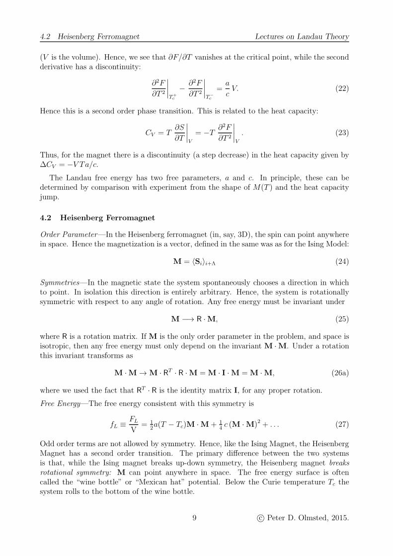
Odd order terms are not allowed by symmetry. Hence, like the Ising Magnet, the HeisenbergMagnet has a second order transition. The primary difference between the two systemsis that, while the Ising magnet breaks up-down symmetry, the Heisenberg magnet breaksrotational symmetry: M can point anywhere in space. The free energy surface is oftencalled the “wine bottle” or “Mexican hat” potential. Below the Curie temperature Tc thesystem rolls to the bottom of the wine bottle.


4.3 Nematic Liquid Crystals Lectures on Landau Theory

Mexican Hat Potential

Once the system has broken symmetry, the further behavior at a given temperature(under, say, the action of a small perturbing field) is much different than that of the Isingmagnet. While the Ising magnet can change only its magnitude, the Heisenberg magnetcan change both magnitude and direction. From the shape of the potential we can seethat changes in magnitude run up the side of the wine bottle, while changes in direction runaround the bottom of the wine bottle and cost no energy! Hence the response, and elasticity,of the broken symmetry state is dominated by the “soft” modes around the wine bottle.This is a general feature of all systems which spontaneously break continuous symmetries,including the big bang! It is arguably one of the most important principles in the universe.The curvature up the side of the wine bottle is often called a “mass”, and in the context ofthe big bang may have something to do with real physical mass.

4.3 Nematic Liquid Crystals

The Isotropic-Nematic transition is an excellent example because, in addition to tellingus about the liquid crystal system, it contains many general features of first order phasetransitions (liquid-gas, liquid-crystal, etc).

Order Parameter—In nematic liquid crystals, rodlike molecules develop an orientation inspace, along an arbitrary direction called the director, n. We have already mentioned that auseful scalar order parameter for this transition is the average 〈P2(cos θ)〉. However, this isnot a useful order parameter since it is not obvious how to deal with the rotational symmetry.It is more useful to consider the mean of the orientation vectors νi for all rods. Since rodsare assumed to have up-down symmetry (i.e. they look the same [unlike magnetic spins]),the order parameter itself must be invariant under ν → −ν. Hence we need somethingquadratic in ν. We will use the following tensor order parameter,

Qαβ = 〈νανβ − 13δαβ〉Λ, (28)



where δαβ is the identity tensor. As before, this is defined within a volume of order Λ3, muchlarger than a molecular volume. For an isotropic distribution of rods all orientations areuncorrelated, so that 〈νανβ〉 vanishes unless α = β = x, y, z, in which case all directions areequally probable, νανα = 1

3. Hence, Q vanishes in the isotropic state and is non-zero in the

nematic state.

Note that the trace of Q, defined as the sum of all diagonal elements, vanishes:

TrQ ≡∑

α

Qαα = 〈ν · ν − 13· 3〉 = 0. (29)

Hence, although Q has three eigenvalues, only two are independent because of the tracecondition. The most general form of Q is:

Q =

−1

3S1 + S2 0 00 −1

3S1 − S2 0

0 0 23S1

≡ S1(n n− 1

3I) + S2(m m− l l). (30)

If S2 = 0 the system is uniaxial, with principal axis of alignment n, and S1 = 〈P2(cos θ)〉.For S2 6= 0 the system is biaxial, with m and l the major and minor axes of alignment in theplane normal to n. Note that l = n×m, so there are two independent axes (hence biaxial).

Symmetries—There are two relevant symmetries to think of for the order parameter.

1. (Lack of) inversion symmetry. Consider a uniaxial state:

Q =

−1

3S1 0 00 −1

3S1 0

0 0 23S1

(prolate uniaxial) (31)

Under inversion,

−Q =

13S1 0 00 1

3S1 0

0 0 −23S1

(oblate uniaxial). (32)

Hence the degree of order is qualitatively different under Q → −Q, and odd invariantsare allowed in the free energy.

2. In a homogeneous isolated system the direction of nematic order is arbitrary; that is,the system and therefore the free energy is rotationally invariant. Q behaves like atensor under rotation, because it is a dyad of unit vectors which rotate as usual. Hencean arbitrary rotation, for which

Qαβ −→ RαλRβρQλρ, (33)

must leave the free energy invariant. For a 3D tensor Q, there are two non-trivialinvariants (corresponding to the two independent eigenvalues), TrQ2 and TrQ3. Under



a rotation,

TrQ ·Q = Qαβ Qβα → RαλRβρQλρRβµRαν Qµν (34a)

= (RTR)νλ (RTR)µρQλρQµν (34b)

= δνλ δµρQλρQµν (34c)

= QνµQµν (34d)

= TrQ · Q, (34e)

and similarly for any power TrQn.

Free Energy—Respecting the invariants, the free energy is

fL = 12a (T − T∗) TrQ

2 + 13bTrQ3 + 1

4c(TrQ2

)2. (35)

We can now insert the general form of Q, Eq. (30), into the free energy, and minimize overS1 and S2. We need to compute quantities such as

TrQ2 = S21 Tr

(nn− 1

3I

)2

+ 2S1S2Tr

(nn− 1

3I

)·(m m− l l

)+ S2

2 Tr(m m− l l

)2

= 13S21 Tr[nn+ 1

3I]− 2

3S1S2Tr

(m m− l l

)+ S2

2 Tr[m m+ l l] (36a)

= 23S21 + 2S2

2 , (36b)

using properties of unit vectors and the orthonormal system {n, m, l}. The free energyreduces to (up to algebraic errors!)

fL = 13a(T − T∗)S

21 +

227b S3

1 +19c S4

1︸︷︷︸F1

+S22

[a(T − T∗)− 4

3b S1 +

23c S2

2

]+ c S4

2︸︷︷︸F2

. (37)

Order Parameter S1

Fre

e E

nerg

y

TIN

Thermodynamics In principle we must look for minima of fL as a function of S1 and S2. F1

gives, for S2 = 0, a minima at T > T∗ for bS1 negative, due to the cubic term. This will



make the term in square brackets in F2 positive, so the system is stable against S2 becomingnon-zero, and is in fact a uniaxial state. So, we consider S2 = 0 and minimize over S1:

∂F1

∂S1

∣∣∣∣S2=0

= 0 −→ S∗1 =

01

4c

[−b±

√b2 − 24ac

].

(38)

By inspection, we take the root with the largest magnitude; now we must change the tem-perature until the free energy at S1∗ vanishes, at which point the system makes a first orderphase transition to the nematic state. (Somewhat tedious) algebra gives:

S1∗ = − b

6c, ∆T = TIN − T∗ =

b2

27ac. (39)

If want a prolate uniaxial state we must have S1 positive, in which case we must chooseb < 0. Conventionally, then, the Landau Free energy for a nematic liquid crystal is usuallywritten as fL = . . .− 1

3bTrQ3+ . . ., with b > 0. We’ll continue here, however, with a general

b. Substituting into the free energy, we find

f = f0 +

{0 (T > TIN)12a(T − T∗)S

21∗ + . . . (T ≤ TIN).

(40)

The free energy is continuous at TIN , but has a kink. This kink is related to the entropychange, for we can calculate

S

V= − ∂f

∂T= −∂f0

∂T+

{0 (T > TIN)∂∂T

{12a(T − T∗)S

21∗ + . . .

}(T ≤ TIN ).

(41)

Hence the entropy change upon cooling through the transition temperature is

∆S = ST=T−IN

− ST=T+

IN= − b4

729 a c3(42)

The entropy of the system decreases, which is the latent heat L = TIN∆S liberated uponcooling into the nematic state.

Notes:

1. Like the magnet, the liquid crystal spontaneously breaks rotational symmetry, with adirection (director) n chosen at random by the system.

2. The Landau free energy for a first order transition is not strictly correct just belowthe transition, since the order parameter grows from a finite value. Hence all resultscan only be qualitative at best, even within mean field theory. Conversely, the Landauenergy for a second order transition is exact, within mean field theory, close to thetransition.

3. There are three parameters, a, b, c, T∗, which can be fitted from experiment by measur-ing, for example, TIN , S1∗,∆T , and the latent heat. ∆T can be measured from lightscattering far above TIN .


4.4 Crystal Systems Lectures on Landau Theory

4. Other mean field first order phase transitions also typically have a cubic term (e.g.most crystal phases).

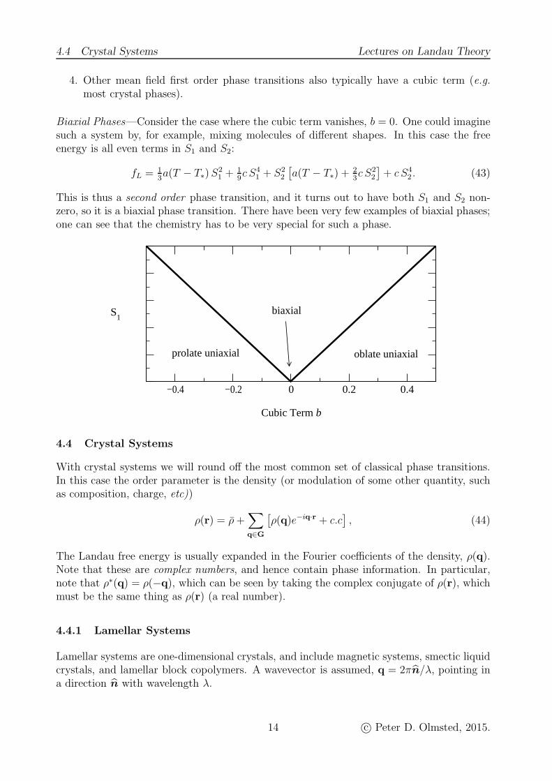
Biaxial Phases—Consider the case where the cubic term vanishes, b = 0. One could imaginesuch a system by, for example, mixing molecules of different shapes. In this case the freeenergy is all even terms in S1 and S2:

fL = 13a(T − T∗)S

21 +

19c S4

1 + S22

[a(T − T∗) +

23c S2

2

]+ c S4

2 . (43)

This is thus a second order phase transition, and it turns out to have both S1 and S2 non-zero, so it is a biaxial phase transition. There have been very few examples of biaxial phases;one can see that the chemistry has to be very special for such a phase.

−0.4 −0.2 0 0.2 0.4

Cubic Term b

S1

prolate uniaxial oblate uniaxial

biaxial

4.4 Crystal Systems

With crystal systems we will round off the most common set of classical phase transitions.In this case the order parameter is the density (or modulation of some other quantity, suchas composition, charge, etc))

ρ(r) = ρ+∑

q∈G


], (44)

The Landau free energy is usually expanded in the Fourier coefficients of the density, ρ(q).Note that these are complex numbers, and hence contain phase information. In particular,note that ρ∗(q) = ρ(−q), which can be seen by taking the complex conjugate of ρ(r), whichmust be the same thing as ρ(r) (a real number).

4.4.1 Lamellar Systems

Lamellar systems are one-dimensional crystals, and include magnetic systems, smectic liquidcrystals, and lamellar block copolymers. A wavevector is assumed, q = 2πn/λ, pointing ina direction n with wavelength λ.



Order Parameter—The order parameter is taken to be the single Fourier mode ρ(q). Otherharmonics will be stabilized at lower temperatures. This is an assumption, and in some casesone could have, due to the microscopic physics, a coincidence of transition temperatures forseveral harmonics.

Symmetries—The only relevant symmetry is translational invariance. Although we will seethat the lamellar state breaks translational invariance, the lamellae can be slid anywhere, andthe high temperature state has no preferred point of reference. Under translation r → r+a,the density transforms to

ρ(r) → ρ(r + a) = ρ+∑

q∈G

[ρ(q)e−iq·r−iq·a + c.c

]. (45)

Hence we have ρ(q) → ρ(q)e−iq·a. That is, all Fourier modes pick up a phase shift. For thefree energy to possess translational invariance, there can be no dependence on the complexphase of the Fourier modes.

Free Energy—So, we now expand in a single Fourier mode. The lowest order expansion ofthe Landau free energy is

fL =1

2a(T − Tc)ρqρ−q +

1

4b (ρqρ−q)

2 (46a)

=1

2a(T − Tc) |ρq|2 +

1

4b |ρq|4 . (46b)

Since the free energy only depends on the modulus of ρ(q), there is no dependence onthe phase. There is no cubic term, since we always assume an analytic expansion of thefree energy, which precludes terms like |ρ(q)|3/2. Hence, one-dimensional crystals are, withinmean field theory, continuous transitions, with spontaneously broken translational symmetry.That is, the direction is arbitrary, as is the phase of the lattice. We will see later that thistransition is ripe for all sorts of interesting fluctuation effects.

4.4.2 Two and Three Dimensional Crystals

Order Parameter— Consider first a 2-dimensional hexagonal crystal. In this case there arethree wavevectors in the first harmonic G∗ = {q1,q2,q3}, of equal magnitude and at relativeangles of 60◦ and 120◦ degrees. They form a star of wavevectors. The Landau free energyfor the transition to a hexagonal crystal must thus be expanded in this star:

ρ(r) = ρ+∑

q∈G∗


], (47)

Free Energy—As with the lamellar crystal, the free energy must be constructed so thatit is translationally invariant, and doesn’t depend on the absolute position of the lattice.Consider the transformation of the following terms under a translation, r → r+ a:

ρk1ρk2

−→ ρk1ρk2

e−i(k1+k2)·a (48a)

ρk1ρk2

ρk3−→ ρk1

ρk2ρk3

e−i(k1+k2+k3)·a (48b)

ρk1ρk2

ρk3ρk4

−→ ρk1ρk2

ρk3ρk4

e−i(k1+k2+k3+k4)·a (48c)



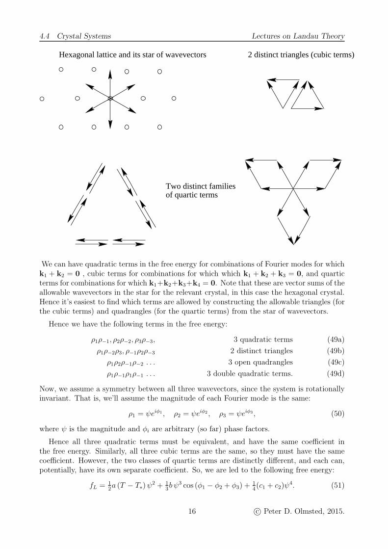
Hexagonal lattice and its star of wavevectors 2 distinct triangles (cubic terms)

Two distinct familiesof quartic terms

We can have quadratic terms in the free energy for combinations of Fourier modes for whichk1 + k2 = 0 , cubic terms for combinations for which which k1 + k2 + k3 = 0, and quarticterms for combinations for which k1+k2+k3+k4 = 0. Note that these are vector sums of theallowable wavevectors in the star for the relevant crystal, in this case the hexagonal crystal.Hence it’s easiest to find which terms are allowed by constructing the allowable triangles (forthe cubic terms) and quadrangles (for the quartic terms) from the star of wavevectors.

Hence we have the following terms in the free energy:

ρ1ρ−1, ρ2ρ−2, ρ3ρ−3, 3 quadratic terms (49a)

ρ1ρ−2ρ3, ρ−1ρ2ρ−3 2 distinct triangles (49b)

ρ1ρ2ρ−1ρ−2 . . . 3 open quadrangles (49c)

ρ1ρ−1ρ1ρ−1 . . . 3 double quadratic terms. (49d)

Now, we assume a symmetry between all three wavevectors, since the system is rotationallyinvariant. That is, we’ll assume the magnitude of each Fourier mode is the same:

ρ1 = ψeiφ1 , ρ2 = ψeiφ2 , ρ3 = ψeiφ3 , (50)

where ψ is the magnitude and φi are arbitrary (so far) phase factors.

Hence all three quadratic terms must be equivalent, and have the same coefficient inthe free energy. Similarly, all three cubic terms are the same, so they must have the samecoefficient. However, the two classes of quartic terms are distinctly different, and each can,potentially, have its own separate coefficient. So, we are led to the following free energy:

fL = 12a (T − T∗)ψ

2 + 13b ψ3 cos (φ1 − φ2 + φ3) +

14(c1 + c2)ψ

4. (51)



In a purely phenomenological approach we might as well set c1+c2 = c, another arbitraryconstant‡. In some systems (notably block copolymers) c1 and c2 can be calculated from“first principles”, assuming Gaussian chains. The phase factors are chosen to minimize thefree energy: choosing φ1 − φ2 + φ3 = 0 gives the largest magnitude for the cosine, so thecubic term can then contribute to the free energy for a non-zero ψ (note that the sign of ψdoesn’t have any physical significance). Note that the phase factors cannot be determinedto any more precision: higher order terms in the free energy lead to a unique determinationof the relative phases.

Notes—

1. All real three dimensional crystals have first order phase transitions because “triangles”can be made. Note that a 2D square lattice has, within mean field theory, a continuousphase transition!

2. One expects single-starred crystals (i.e. square instead of rectangular, hexagonal in-stead of rhombic) to appear from the melt, since these will typically be triggered by thefirst length scale which becomes unstable. For deeper quenches, or strong first orderphase transitions, other harmonics develop.

3. By counting the number of triangles, essentially, one can make a very beautiful andgeneral argument that most simple substances should become BCC crystals immedi-ately from the melt§. This simple rule is obeyed astonishingly often!

4. An excellent example of this approach combined with a derivation of the Landau coef-ficients is Leibler’s treatment of microphase separation in block copolymers¶. He pre-dicted the stability of BCC, hexagonal, and lamellar phases from a single-star theory.Enlarging the theory to include the second star (harmonic) can predict the stability ofthe Gyroid phase‖

‡For higher order terms the different classes of pentangles, sextangles, etc could have different phasefactors, in which case the corresponding coefficients should be kept distinct.

§S. Alexander and J. McTague, “Should all crystals be bcc? Landau theory of solidification and crystalnucleation”, Phys. Rev. Lett. 41 (1978) 702-705

¶L. Leibler, “Theory of Microphase Separation in Block Copolymers”, Macromolecules 13 (1980) 1602-1617

‖S. T. Milner and P. D. Olmsted, “Analytical weak-segregation theory of bicontinuous phases in diblockcopolymers”, J. Phys. II (France) 7 (1997) 249-255.


5. Smectic Liquid Crystals Lectures on Landau Theory

5 Smectic Liquid Crystals

5.1 Mean Field Theory of the Nematic-Smectic–A transition

A thermotropic smectic liquid crystal has the symmetry of a one-dimensional lamellar crystal,but suffers the complications of occuring out of a nematic phase which has broken rotationalsymmetry. In the smectic–A phase the rodlike molecules are, on average, parallel to thelayer normals. Hence the director, n(r), is parallel to the layer normal.

Order Parameter—The order parameter of the smectic transition is taken to be the Fouriercomponent of the fundamental harmonic of the one-dimensional crystal; i.e. we expand thedensity as

ρ(r) = ρ+{ψe−iq n·r + ψ∗eiq n·r

}, (52)

where n is both the director and the definition of the layer normals.

n

z

x

θn

Symmetries— The layers can be oriented in any direction, as long as the director is alsopointing in that direction. Hence any smectic free energy that we write down must beinvariant under simultaneous rotations of the layers and the director. Under a uniformrotation of a smectic system about the y axis by an angle θ, the director changes:

n −→ n′ = n+ δn = n− θ x. (53)

Hence the smectic order parameter changes according to:

ψ −→ ψeiq θx = ψe−iqx δnx . (54)

Any free energy we write down my respect this symmetry (rotational invariance).

Free Energy—Now we write down the free energy. First we consider a uniform amplitude ofthe density modulation ψ. Since a smectic is a one-dimensional crystal, we can reproducewhat we had before:

fL,hom = 12a(T − Tc) |ψ|2 + 1

4c |ψ|4 . (55)

To this we add the energy of deformation of the director fluctuations, the Frank Free Energy:

fN = 12K1 (∇ · δn)2 + 1

2K2 (n ·∇× δn)2 + 1

3K3 |n× (∇× δn)|2 , (56)


5.2 Free Energy and Superconducting Analogy Lectures on Landau Theory

where K1, K2, K3 penalize, respectively, splay, bend, and twist fluctuations.

Finally, we can consider an envelope of spatial modulations in the magnitude of the densitymodulation, ψ(r). These fluctuations, in the smectic state, correspond to phonons. If weconsider the rigid body rotation above, transverse spatial derivatives of ψ pick up a termfrom the director rotation:

∂xψ(r) −→︸︷︷︸(rotate about y)

(∂xψ) e−iq xδnx + iq δnx ψ(r) e

−iq xδnx . (57)

Since the free energy must be invariant under a rigid body rotation, such spatial deriva-tives must not contribute to the free energy. Hence the free energy of deforming the orderparameter is

fL,def =12g‖ |n ·∇ψ|2 + 1

2g⊥ |(∇⊥ − iqδn) ψ|2 . (58)

The additional term in parentheses in the second terms subtracts off the unwanted irrelevantterm. This derivative is often called a covariant derivative, and has an analogy in super-conductivity, in which the superconductor is analogous to the smectic order parameter andthe vector potential is analogous to the director fluctuations. This is an example of a gaugefield theory, which arises when the relevant order parameter has a local internal symmetry(the smectic order parameter is a complex number with a phase, corresponding to a U(1)symmetry, which can vary from point to point). There have been many interesting fruitsborn out of this analogy between smectics and superconductors! In electrodynamics thereis a gauge symmetry (the vector potential A is defined only up to an additive irrotationalvector field ∇Θ), while in the smectic liquid crystal the gauge is actually fixed because ofthe presence of a director in the nematic state.

5.2 Free Energy and Superconducting Analogy

To compare the liquid crystals and superconductors, let’s look at the free energies. For theliquid crystal we have

fNA = 12a |ψ|2 + 1

4c |ψ|4 + 1

2g‖ |n ·∇ψ|2 + 1

2g⊥ |(∇⊥ − iqδn) ψ|2 + 1

2K (∇αδnβ)

2 , (59)

where we have used the so-called one-constant approximation K1 = K2 = K3 ≡ K.

For a superconductor, we’ll take the order parameter to be ψ again. Landau postulatedthat this is a complex number, and in fact it turns out to be closely related to the wavefunc-tion for Cooper pairs of electrons (which is a complex number). The physics of electronsis invariant under a local change in the phase of the wavefunction, ψ(r) → ψ(r)eiφ(r). Thistransformation is in fact the gauge invariance which gives rise to the electromagnetic field,and we usually write

ψ(r) → ψ(r)ei2e

∫r

r0A·dr′

, (60)

where A is the electromagnetic vector potential (this funny phase factor gives rise to theAharonov-Bohm effect), in units where the speed of light is unity. There is a 2 here becausethe wavefunction is for a pair of electrons. Now, we can write down the free energy for asuperconducting transition, exactly as for the smectic. When it comes to writing the gradientterms we must “subtract” off this arbitrary phase, which can’t change the physics, so gradient


5.2 Free Energy and Superconducting Analogy Lectures on Landau Theory

operators generally enter as ~∇− i2eA. Finally, there is a free energy associated with gaugefield fluctuations: the energy in the magnetic field is B · B/8π. Writing B = ∇ × A, wehave, for the superconducting free energy,

fsup =12a |ψ|2 + 1

4c |ψ|4 + 1

2g

∣∣∣∣(∇− i

2e

~A

)ψ

∣∣∣∣2

+c2

8π|∇×A|2 . (61)

Hence, aside from the fact that the liquid crystal is anisotropic, and the coupling of A to thegradient terms is slightly different in tensorial nature to the coupling of δn, the transitions“should” be qualitatively the same. Just as a superconductor expels magnetic flux, a liquidcrystal expels (it turns out) both twist and bend director fluctuations. For example, it wasrealized that the analog of the Abrikosov vortex phase of Type II superconductors shouldexist in liquid crystals, and this was subsequently predicted and then found experimentally:the “twisted grain boundary (TGB) phase” in cholesteric smectics.

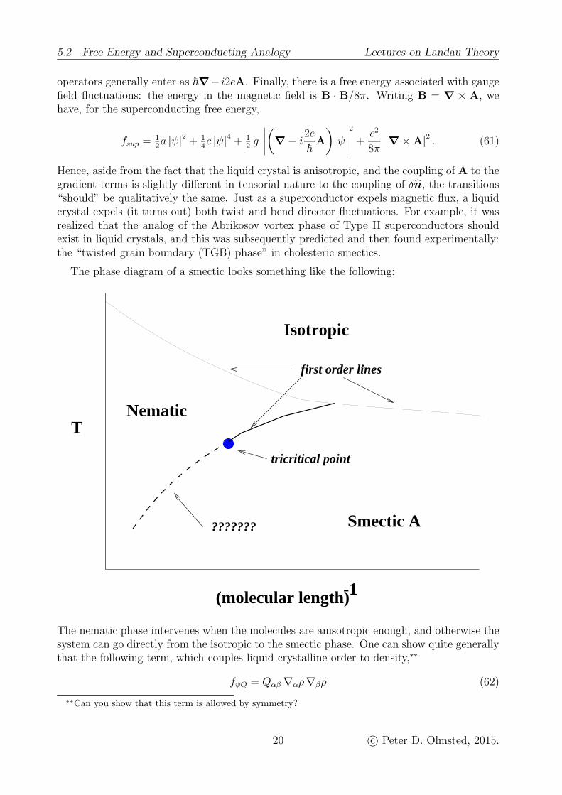
The phase diagram of a smectic looks something like the following:

Isotropic

TNematic

???????

first order lines

tricritical point

Smectic A

-1(molecular length)

The nematic phase intervenes when the molecules are anisotropic enough, and otherwise thesystem can go directly from the isotropic to the smectic phase. One can show quite generallythat the following term, which couples liquid crystalline order to density,∗∗

fψQ = Qαβ ∇αρ∇βρ (62)

∗∗Can you show that this term is allowed by symmetry?


5.3 Fluctuations and the Halperin-Lubensky-Ma Effect. Lectures on Landau Theory

leads (via nematic fluctuations) to an effective quartic term in the smectic free energy ofthe form −χψ4, where χ is the susceptibility for fluctuations around the nematic phase.Hence, it is likely that for molecular parameters with a narrow nematic range, for which thesusceptibility χ is large, the total quartic term in the smectic free energy is negative, leadingto a first order phase transition. For parameters with a wide nematic range the N − Atransition is expected, within mean field theory, to be a continuous transition. In the nextsection we will see that this does not, generally, survive inclusion of fluctuations.

5.3 Fluctuations and the Halperin-Lubensky-Ma Effect.

In the region of the smectic transition both ψ and δn are fluctuating. If we consider afluctuation in which a smectic blob appears in the nematic, there are two relevant lengthscales:

ξ‖,⊥ =

√g‖,⊥a

(ψ healing length) (63)

λ =

√K

g‖,⊥q20|ψ|2(bend and twist penetration lengths) (64)

The Frank constant K is proportional to the magnitude of the nematic order parameter Q,so λ is large when the nematic phase has a large range and smaller when the nematic rangeis smaller. Hence we expect two regimes:

κ ≡ λ

ξ

<1√2

(Type I)

>1√2

(Type II)(65)

In the Type I case the director fluctuation (or magnetic field) decays quickly compared tothe smectic order parameter, and the system can efficiently expel twist (or magnetic field).This corresponds to the Meissner phase in superconductors. In the Type II case the twistcan penetrate a longer distance while order parameter has healed, and can in fact penetrateeasier. This corresponds to the Abrikosov vortex phase in superconductors.

If we consider fluctuations in the nematic phase, in the Type I limit we can safely assumethat ψ is uniform relative to director fluctuations (since ψ varies much more smoothly). Toexamine the smectic transition in this limit, then, we consider small (uniform) fluctuationsin ψ, and integrate out the director fluctuations. Hence:

Z =

∫DδnDψ e{

∫d3rfNA/kBT} (66)

≃∫

DδnDψ exp

{− V

kBT

[12a |ψ|2 + 1

4c |ψ|4

]+ (67)

1kBT

∫d3r

{12g⊥ |(∇⊥ − iq0δn) ψ|2 + 1

2K (∇αδnβ)

2}}, (68)

≃∫

Dψe−V f0NA[ψ]/kBT∫δne−Fnem/kBT (69)


5.4 Layered liquids and the Brazovskii effect Lectures on Landau Theory

where f0NA is the free energy in the absence of director fluctuations, and

Fnem = 12

∫d3r

{g⊥q

20|ψ|2|δn|2 +K (∇αδnβ)

2} . (70)

The director fluctuation integral is Gaussian, and can be done without too much trouble. InFourier space, δn(r) =

∑qδn(q)eiq·r, we can write

Fnem = 12

∑

q

[g⊥q

20|ψ|2|+Kq2

]|δn(q)|2 . (71)

The director integral is a Gaussian integral for each Fourier mode, giving (up to factors of2π) ∫

δne−Fnem/kBT ≃∏

q

[g⊥q

20|ψ|2|+Kq2

]− 1

22

(72)

(a power of 12for each independent mode of δn). Hence the effective free energy for the

smectic transition is

Z =

∫DδnDψ e{

∫d3rfNA/kBT} (73)

=⇒fNA = f0NA + kBT∑

q

ln[g⊥q

20|ψ|2 +Kq2

](74)

This integral can be done (∑

q → 1/(2π)3∫d3q), and expanded in the order parameter ψ.

Note that it can’t be expanded first because the integrand is non-analytic at ψ = 0. Theresult is

fNA = f0NA + a1|ψ|2 −1

6π

(g⊥q

20 |ψ|2K

)3/2

+ a2ψ4 + . . . (75)

Hence, there is a cubic term induced in the magnitude of ψ. This leads to a very weakfluctuation-induced first order transition. This seems to have been verified experimentally(most people agree).

In the case of Type II systems, where director and order parameter fluctuations (or mag-netic field and superconducting order parameter), a renormalization group type of treatmentis necessary. It is believed that the first order transition remains, but results are inconclusive.In any case if it remains first order it is VERY weak!

5.4 Layered liquids and the Brazovskii effect

To be added!


Lectures on Landau Theory of Phase Transitions

Documents

Transcript of Lectures on Landau Theory of Phase Transitions