Lectures on Economic Inequality

Warwick, Summer 2016, Slides 1

Debraj Ray

Overview: Convergence and Divergence

Inequality and Divergence: Economic Factors

Inequality and Divergence: Psychological Factors

Inequality, Polarization and Conflict

Uneven Growth and Conflict

0-0

Convergence and Divergence

Cross-country:

Solow

Within-country:

Kuznets

0-1

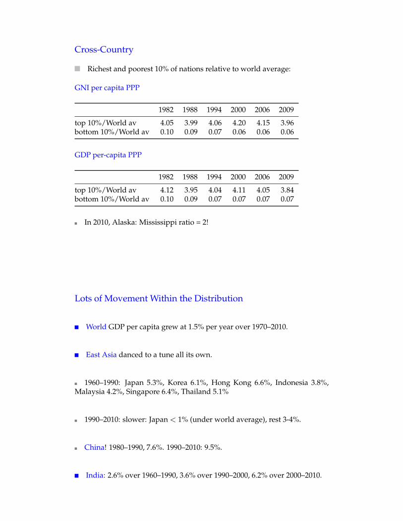
Cross-Country

Richest and poorest 10% of nations relative to world average:

GNI per capita PPP

1982 1988 1994 2000 2006 2009

top 10%/World av 4.05 3.99 4.06 4.20 4.15 3.96bottom 10%/World av 0.10 0.09 0.07 0.06 0.06 0.06

GDP per-capita PPP

1982 1988 1994 2000 2006 2009

top 10%/World av 4.12 3.95 4.04 4.11 4.05 3.84bottom 10%/World av 0.10 0.09 0.07 0.07 0.07 0.07

In 2010, Alaska: Mississippi ratio = 2!

0-2

Lots of Movement Within the Distribution

World GDP per capita grew at 1.5% per year over 1970–2010.

East Asia danced to a tune all its own.

1960–1990: Japan 5.3%, Korea 6.1%, Hong Kong 6.6%, Indonesia 3.8%,Malaysia 4.2%, Singapore 6.4%, Thailand 5.1%

1990–2010: slower: Japan < 1% (under world average), rest 3-4%.

China! 1980–1990, 7.6%. 1990–2010: 9.5%.

India: 2.6% over 1960–1990, 3.6% over 1990–2000, 6.2% over 2000–2010.

0-3

Latin America not too hot (from an economic point of view).

1960–1980: around 2.9% annually.

1980–1990, the “lost decade” for Latin America, decline of over 0.7% yearover year, overall decline of around 10%. Argentina -2.9%, Brazil -0.5%, Mex-ico -0.3%, Peru -3.0%, Uruguay -0.7%.

Only Chile (2.1%) and Colombia (1.4%) had higher per capita income in1990 than they did in 1980.

1990–2010, still slow, around world average (exceptions Chile, 4.7%, andArgentina, 3.6%).

2000–2010: Average well in excess of 2%. Argentina 3.3%, Brazil 2.4%,Chile 2.6%, Peru 4.3%, Uruguay 3.0%. Mexico not so well at 0.8%.

0-4

Sub-Saharan Africa more stagnation.

1980–1990 decline at 1% annual.

1990–2000 decline at 0.4% annual.

2000–2010 better, with growth at 2.2%.

Examples.

Nigeria (-1.6%) and Tanzania (-2.0%) in the 1980s, stagnation 1990s, robustrecovery over 2000–2010 (3.9% Nigeria, 4.0% Tanzania).

Kenya barely grew in the 1980s, declined in the 1990s, some recovery2000–2010; overall 0.2% over 30 years.

0-5

Uganda stagnated over the 1980s (-0.1%) before picking up pace and mak-ing substantial progress over 1990–2010, growing at over 3.5% annually.

Rwanda, crippled by negative growth in the 1980s (-1.2%) and 1990s (-0.7%) before a remarkable recovery over 2000–2010 (4.8%).

Yet Burundi’s negative growth rate of 3.2% in the 1990s made worse bynear-stagnation over 2000–2010 (0.4%).

The Democratic Republic of the Congo in freefall over 1980–1990 (-2.2%)and 1990–2000 (-8.5%!) before 1.8% 2000–2010.

Zimbabwe stagnated in the 1980s (0.7%) and 1990s (-0.3%) before enteringa freefall of its own (-4.8%) over 2000–2010.

0-6

OECD: 20 original members, fourteen additions. All the developed coun-tries, a few middle-income countries also members.

1970–1990, OECD growth a bit over 2.4%

1990–2000 1.8%, a bit higher than world average

2000–2010 Under world average at 0.8%

The United States mirrors OECD reasonably well:

2.2% over 1970–1990

a bit under 2.2% in 1990–2000

0.7% in 2000–2010

0-7

Summary So Far

Over 1980–2010, distribution of world income stable or somewhat wors-ening.

Richest 10% of nations 4 times the world average

Poorest 10% had 6–10% of world average, generally declining.

But lots of movement within the distribution.

Rise of Asia: Japan, then China and now India

Languishing of sub-Saharan Africa

Relatively slow growth in many parts of Latin America

0-8

Within-Country

Inter-country inequality compounded within countries:

0–4,000 PPP (2000):

Country GDP pc (c. 2000) Share bot. 40% Share top 20%

Malawi 546 13 56Uganda 765 16 50Tanzania 866 19 42Bangladesh 893 22 40Senegal 1,492 17 48Pakistan 1,898 21 42Nicaragua 2,157 12 55Sri Lanka 3,106 17 48Bolivia 3,402 7 63Guatemala 3,350 11 59

0-9

Within-Country

Inter-country inequality compounded within countries:

4,000–13,000 PPP (2000):

Country GDP pc (c. 2000) Share bot. 40% Share top 20%

El Salvador 5,183 10 55Peru 5,444 11 57Costa Rica 5,520 13 50Thailand 5,568 11 59Panama 5,840 8 60Colombia 6,617 9 61Brazil 7,911 7 65Costa Rica 8,113 13 51Venezuela 9,924 12 52Mexico 12,095 12 56

0-10

Within-Country

Inter-country inequality compounded within countries:

13,000+ PPP (2000):

Country GDP pc (c. 2000) Share bot. 40% Share top 20%

Korea 16.015 21 37Spain 25,129 19 42UK 28,575 18 44Sweden 29,126 23 37Switzerland 34,713 20 41USA 39,578 16 46Norway 43,642 24 37

0-11

Some Lorenz Curves

!! !

! !

"!#!

$!%&!

'#!

#'!

('!

)#!

&)!

*$!

%""!

"!

'"!

("!

&"!

+"!

%""!

"! '"! ("! &"! +"! %""!

!"#"$%&'()*+,%-)+*./*'01.#

)*23

4*

!"#"$%&'()*+,%-)+*./*5.5"$%&'.0*234*

6)-#%07*

"!(!

$!%&!

'#!

#%!

(%!

)'!

&(!

*$!

%""!

"!

'"!

("!

&"!

+"!

%""!

"! '"! ("! &"! +"! %""!

!"#"$%&'()*+,%-)+*./*'01.#

)*23

4*

!"#"$%&'()*+,%-)+*./*5.5"$%&'.0*234*

8-%01)*

0-12

Some Lorenz Curves

!! !

! !

"! #!$!

#"!#%!

&'!

('!

'$!

$)!

*$!

"!

&"!

'"!

%"!

)"!

#""!

"! &"! '"! %"! )"! #""!

!"#"$%&'()*+,%-)+*./*'01.#

)*23

4*

!"#"$%&'()*+,%-)+*./*5.5"$%&'.0*234*

6.-)%7*8)5"9$'1*./*

"! &!%!

##!#*!

&$!

('!

'$!

$)!

*(!

#""!

"!

&"!

'"!

%"!

)"!

#""!

"! &"! '"! %"! )"! #""!

!"#"$%&'()*+,%-)+*./*'01.#

)*23

4*

!"#"$%&'()*+,%-)+*./*5.5"$%&'.0*234*

:.-;%<*

0-13

Some Lorenz Curves

!! !

! !

"! #!$!

%!&'!

#"!#(!

)*!

'(!

*)!

&""!

"!

#"!

'"!

*"!

+"!

&""!

"! #"! '"! *"! +"! &""!

!"#"$%&'()*+,%-)+*./*'01.#

)*23

4*

!"#"$%&'()*+,%-)+*./*5.5"$%&'.0*234*

6-'*7%08%*

"! #! '!+!

&)!&%!

#*!

)$!

'(!

*'!

&""!

"!

#"!

'"!

*"!

+"!

&""!

"! #"! '"! *"! +"! &""!!"

#"$%&'()*+,%-)+*./*'01.#

)*23

4*!"#"$%&'()*+,%-)+*./*5.5"$%&'.0*234*

9)-"*

0-14

Some Lorenz Curves

!! !

! !

"! #! $!%!

#&!#%!

&'!

($!

$'!

)#!

#""!

"!

&"!

$"!

)"!

%"!

#""!

"! &"! $"! )"! %"! #""!

!"#"$%&'()*+,%-)+*./*'01.#

)*23

4*

!"#"$%&'()*+,%-)+*./*5.5"$%&'.0*234*

6)7'1.*

"! &! $!%!

#&!#%!

&'!

((!

$'!

)#!

"!

&"!

$"!

)"!

%"!

#""!

"! &"! $"! )"! %"! #""!

!"#"$%&'()*+,%-)+*./*'01.#

)*23

4*

!"#"$%&'()*+,%-)+*./*5.5"$%&'.0*234*

6%$%8+'%*

0-15

Some Lorenz Curves

!! !

! !

"! #! $! %!&!

#'!("!

()!

$&!

**!

#""!

"!

("!

'"!

%"!

)"!

#""!

"! ("! '"! %"! )"! #""!

!"#"$%&'()*+,%-)+*./*'01.#

)*23

4*

!"#"$%&'()*+,%-)+*./*5.5"$%&'.0*234*

6-%7'$*

"! #! $! %!&!

#'!#&!

(%!

$%!

*"!

"!

("!

'"!

%"!

)"!

#""!

"! ("! '"! %"! )"! #""!!"

#"$%&'()*+,%-)+*./*'01.#

)*23

4*!"#"$%&'()*+,%-)+*./*5.5"$%&'.0*234*

!,'$)*

0-16

Some Lorenz Curves: Consumption Data

!! !

! !

"!

#!

$$!

%&!

'&!

(""!

"!

$"!

)"!

*"!

&"!

(""!

"! $"! )"! *"! &"! (""!

!"#"$%&'()*+,%-)+*./*'01.#

)*23

4*

!"#"$%&'()*+,%-)+*./*5.5"$%&'.0*234*

6785&*

"!

&!

(#!

%)!

''!

(""!

"!

$"!

)"!

*"!

&"!

(""!

"! $"! )"! *"! &"! (""!

!"#"$%&'()*+,%-)+*./*'01.#

)*23

4*

!"#"$%&'()*+,%-)+*./*5.5"$%&'.0*234*

90:'%*

0-17

Some Lorenz Curves: Consumption Data

!! !

"!

#!

$%!

&'!

(&!

$""!

"!

'"!

)"!

*"!

%"!

$""!

"! '"! )"! *"! %"! $""!

!"#"$%&'()*+,%-)+*./*'01.#

)*23

4*

!"#"$%&'()*+,%-)+*./*5.5"$%&'.0*234*

607.0)+'%*

"!(!

$(!

'+!

($!

$""!

"!

'"!

)"!

*"!

%"!

$""!

"! '"! )"! *"! %"! $""!!"

#"$%&'()*+,%-)+*./*'01.#

)*23

4*!"#"$%&'()*+,%-)+*./*5.5"$%&'.0*234*

8'9)-'%*

0-18

Inequality and per-capita income: the whole range

!"#

$%#

$"#

%%#

%"#

&%#

&"#

'%#

'"#

(%#

)# ')))# !))))# !')))# $))))# $')))# %))))# %')))# &))))# &')))#

!"#$"%

&'(")*%

$+,")-.'#"/)

01!)2"#)$'23&')'#+4%5)6777)

*+,-.#/01#$)2#

*+,-.#30405#&)2#

0-19

Inequality and per-capita income: up to $8000, an inverted-U?

!"

#!"

$!"

%!"

&!"

'!"

(" $(((" &(((" !(((" )(((" #((((" #$(((" #&((("

!"#$%&

'()%*+&

$,-%*./(#%0*

12!*3%#*$(34'(*(#,5&6*7888*

*+,-."/01"$(2"

*+,-."30405"&(2"

0-20

Uneven and Compensating Changes

Uneven growth, perhaps from a few sectors

Then other sectors catch up, or people migrate

Tends to generate an inverted-U, but no inevitability to it.

Note: our diagram was on the cross-section.

In fact, rising inequality in many countries (coming up!).

0-21

Two Parallel Literatures

Cross-country convergence

Within-country narrowing of inequality

Both literatures have been caught wrong-footed.

0-22

Cross-Country: Testing Convergence

1. Baumol (AER 1986): 16 countries, among the richest in the world today.

In order of poorest to richest in 1870: Japan, Finland, Sweden, Norway,Germany, Italy, Austria, France, Canada, Denmark, the United States, theNetherlands, Switzerland, Belgium, the United Kingdom, and Australia.

Angus Maddison: per-capita incomes for 1870.

Idea: regress 1870–1979 growth rate on 1870 incomes.

ln y1979i � ln y1870

i = A+ b ln y1870i + ✏i

Unconditional convergence ) b ' �1.

Get b = �0.995, R2 = 0.88.

0-23

What’s wrong with this picture?

0-24

De Long critique (AER 1988):

Add seven more countries to Maddison’s 16.

In 1870, they had as much claim to membership in the “convergence club”as any included in the 16: Argentina, Chile, East Germany, Ireland, NewZealand, Portugal, and Spain.

New Zealand, Argentina, and Chile were in the list of top ten recipients ofBritish and French overseas investment (in per capita terms) as late as 1913.

All had per capita GDP higher than Finland in 1870.

Strategy: drop Japan (why?), add the 7.

0-25

Slope still negative, though loses significance.

Correct for measurement error, game over.

0-26

2. More Countries

2a. Updated Maddison dataset 2013, 60 countries:

1"

2"

3"

4"

5.8" 6.3" 6.8" 7.3" 7.8"

log"pe

r1capita"income"grow

th,"187012010"

log"per1capita"income,"1870"(in"1990"dollars)"

0-27

2b. Even More Countries.

Barro (QJE 1991): 100+ countries over 1960–1985.

0-28

2c. Even More Countries + Long Time Horizon (Pritchett)

What about more countries and more time?

Problem: no data going back to 1870.

Pritchett assumption: no country can fall below $250 per capita (1985 PPP)

Defense 1: lowest 5-year average ever is Ethiopia $275 (1961–5).

Defense 2: below extreme nutrition-based poverty lines actually used inpoor countries (see Ravallion, Dutt and van de Valle 1991, or nutrition linesat 2000Kcal)

Defense 3: at any lower income, population too unhealthy to grow. Childmortality rate estimated to climb well above barrier of 600 per 1000.

0-29

Claim: the $250 bound “proves” divergence over long-run.

The US grew four-fold from 1870 to 1960.

Thus, any country whose income was not fourfold higher in 1960 than itwas in 1870 grew more slowly than the United States.

42 out of 125 countries in the PWT have pcy below $1,000 in 1960.

Or try this:

extrapolate back so poorest country in 1960 hits exactly $250 in 1870.

US: use actual figures.

preserve the relative rankings of all other countries (see footnote 11 ofPritchett)

0-30

0-31

Mobility matrix, 1982–2009

Cat 1: income < 1/4 world av; Cat 2: between 1/4 and 1/2 world av; Cat3: between 1/2 world av and world av; Cat 4: between world av and twiceworld av; Cat 5: income > twice world av.

Obs Cat ¿ ¡ ¬ √ ƒ32 ¿ 84 13 3 0 021 ¡ 43 43 14 0 026 ¬ 0 27 50 23 020 √ 0 0 20 70 1029 ƒ 0 0 0 3 97

0-32

Within-Country: The Return of Inequality

The financial crisis sparked a new interest in inequality.

But inequality has been historically high

Growing steadily through late 20th century

Wolff, Piketty, Saez, Atkinson, many others

0-33

25%

30%

35%

40%

45%

50%

1910 1920 1930 1940 1950 1960 1970 1980 1990 2000 2010

Sha

re o

f top

dec

ile in

nat

iona

l inc

ome

Figure I.1. Income inequality in the United States, 1910-2010

The top decile share in U.S. national income dropped from 45-50% in the 1910s-1920s to less than 35% in the 1950s (this is the fall documented by Kuznets); it then rose from less than 35% in the 1970s to 45-50% in the 2000s-2010s. Sources and series: see piketty.pse.ens.fr/capital21c.

Source: Piketty (2014)

0-34

25%

30%

35%

40%

45%

50%

1900 1910 1920 1930 1940 1950 1960 1970 1980 1990 2000 2010

Sha

re o

f top

dec

ile in

tota

l inc

ome

The top decile income share was higher in Europe than in the U.S. in 1900-1910; it is a lot higher in the U.S. in 2000-2010. Sources and series: see piketty.pse.ens.fr/capital21c.

Figure 9.8. Income inequality: Europe vs. the United States, 1900-2010

U.S.

Europe

Source: Piketty (2014)

0-35

0%

2%

4%

6%

8%

10%

12%

14%

16%

18%

20%

22%

24%

1910 1920 1930 1940 1950 1960 1970 1980 1990 2000 2010

Sha

re o

f top

per

cent

ile in

tota

l inc

ome

The share of top percentile in total income rose since the 1970s in all Anglo-saxon countries, but with different magnitudes. Sources and series: see piketty.pse.ens.fr/capital21c.

Figure 9.2. Income inequality in Anglo-saxon countries, 1910-2010

U.S. U.K.

Canada Australia

Source: Piketty (2014)

0-36

0%

1%

2%

3%

4%

5%

6%

7%

8%

9%

10%

11%

12%

1910 1920 1930 1940 1950 1960 1970 1980 1990 2000 2010

Sha

re o

f top

0.1

% in

tota

l inc

ome

The share of the top 0.1% highest incomes in total income rose sharply since the 1970s in all Anglo-saxon countries, but with varying magnitudes. Sources and series: see piketty.pse.ens.fr/capital21c.

Figure 9.5. The top 0.1% income share in Anglo-saxon countries, 1910-2010

U.S. U.K.

Canada Australia

Source: Piketty (2014)

0-37

Why Do We Care?

Inequality is of intrinsic as well as instrumental interest

Intrinsic:

inequality measurement: evaluate and compare distributions

evolution of inequality in societies

Instrumental: connections between inequality and development

inequality and various outcomes: growth, nutrition, employment

inequality and history-dependence

Goal: To study some of these theories and connections.

0-38

A recent book by Piketty

summarizes the evidence (compelling and useful)

describes three “fundamental laws”

is a runaway hit in the United States, touching a raw nerve

0-39

Piketty’s Three Fundamental Laws

The First Fundamental Law:

Capital IncomeTotal Income

=Capital IncomeCapital Stock

⇥Capital StockTotal Income

.

Share of capital income equals rate of return on capital multiplied by thecapital-output ratio.

Useful in organizing our mental accounting system.

But it explains nothing.

0-40

The Second Fundamental Law:

Growth rate equals savings rate divided by capital-output ratio.

investment = savings: I(t) = S(t) = s(t)Y (t)

investment adds to capital stock

K(t+ 1) = [1� �(t)]K(t) + I(t) = [1� �(t)]K(t) + s(t)Y (t)

Convert to growth rates:

G(t) =s(t)

✓(t)� �(t),

where G(t) = [K(t+ 1)�K(t))]/K(t) and ✓(t) = K(t)/Y (t).

Approximate per-capita version: subtract n(t), the rate of population growth.

g(t) 's(t)

✓(t)� �(t)� n(t),

0-41

g(t) 's(t)

✓(t)� �(t)� n(t),

This isn’t a theory unless you take a stand on one or more of the variables.

E.g., as Harrod or Solow did. Piketty doesn’t appear to.

“If one now combines variations in growth rates with variations in savingsrate, it is easy to explain why different countries accumulate very differentquantities of capital, and why the capital-income ratio has risen sharply since1970. One particularly clear case is that of Japan: with a savings rate closeto 15 percent a year and a growth rate barely above 2 percent, it is hardlysurprising that Japan has over the long run accumulated a capital stock worthsix to seven years of national income. This is an automatic consequence of the[second] dynamic law of accumulation.” (p.175)

“The very sharp increase in private wealth observed in the rich countries, andespecially in Europe and Japan, between 1970 and 2010 thus can be explainedlargely by slower growth coupled with continued high savings, using the[second] law . . . ” (p. 183)

0-42

The Third Fundamental Law:

r > g

Piketty: “the central contradiction of capitalism.”

0-43

r > g in the data.

0%

1%

2%

3%

4%

5%

6%

0-1000 1000-1500 1500-1700 1700-1820 1820-1913 1913-1950 1950-2012 2012-2050 2050-2100

Ann

ual r

ate

of re

turn

or r

ate

of g

row

th

The rate of return to capital (pre-tax) has always been higher than the world growth rate, but the gap was reduced during the 20th century, and might widen again in the 21st century.

Sources and series: see piketty.pse.ens.fr/capital21c

Figure 10.9. Rate of return vs. growth rate at the world level, from Antiquity until 2100

Pure rate of return to capital r (pre-tax)

Growth rate of world output g

0-44

Supposedly explains widening inequalities via capital income. Yes or no?

Begin again with the capital accumulation equation:

K(t+ 1) = [1� �(t)]K(t) + s(t)Y (t)

Start disciplining: s(t) = s, �(t) = �, and

Yt = AK✓t [(1+ �)tLt]1�✓,

where Lt grows at rate n, and � is technical progress.

Normalized capital-labor ratio: kt ⌘ Kt/Lt(1+ �)t; then

(1+ n)(1+ �)kt+1 = (1� �)kt + sAk✓t ,

so that kt ! k⇤ '

sA

n+ � + �

�1/(1�✓)

.

This is the Solow model.

0-45

So the overall rate of growth converges to n+ �.

Rate of return on capital is given by the marginal product:

rt = ✓A⇥Kt/(1+ �)tLt

⇤✓�1

= ✓Ak✓�1t

! ✓A

sA

n+ � + �

��1

=✓

s[n+ � + �],

So down to comparing r = ✓s [n+ � + �] with g = n+ �.

Piketty’s Third Law follows if ✓ � s.

Surely true empirically.

Deeper argument: ✓ � s because of the transversality condition.

0-46

s is inefficient if consumption can be improved in all periods.

Easy example: s = 1.

More generally, recall that kt ! k⇤ '

sA

n+ � + �

�1/(1�✓)

.

So per-capita output converges to

A1/(1�✓)(1+ �)t✓

s

n+ � + �

◆✓/(1�✓)

and per-capita consumption converges to the path

A1/(1�✓)(1+ �)t✓

s

n+ � + �

◆✓/(1�✓)

(1� s).

It follows that if s > ✓, the growth path is inefficient.

So efficiency implies r > g, but there is no prediction for inequality.

0-47

Summary

Piketty’s work is pathbreaking in recording the evolution of inequality.

As a theory of inequality, it leaves much to be desired.

In what follows, we study some theories of inequality.

0-48