Lectures on Cellular Automata Continued

Modified and upgraded slides of

Martijn Schutschut@cs.vu.nl Vrij Universiteit Amsterdam

Lubomir IvanovDepartment of Computer ScienceIona College

and anonymous from Internet

Morphogenetic Morphogenetic modeling modeling

Dynamical Systems Dynamical Systems

and Cellular Automataand Cellular Automata

matterheat

matterheat

matterenergymatterenergy

entropy dissipator

Organisms are dissipative processes

in space and time

Dynamical system

Time

Space

S(x , t)

state S atx at time t ?

Energy

Model animals as dynamical systems

Tissues

Groups

Which space? - which geometry?

parameter space

a

b

geometric space

x

y

x2

a2 y2

b2 1

state space

x a cos t

y b sin t

morphometric space

Q=S/A

S

A

?

time

velocity

Which space? - which geometry?

? parameter space

genotypeenvironment

state space

phylogeny/ontogeny

morphometric space

morphology

geometric space

ontogeny/phenotype

GA evolution environment

Dynamics of species in environments.

• discrete time steps T=0,1,2,3,…

• discrete cells at X,Y,Z=0,1,2,3,...

• discretize cell states S=0,1,2,3,...

Discretization has many aspects

t

t+1

t+2We can mix discrete and continuous values in some models

Cellular AutomatonCellular Automaton

t

t+1

update rules

neighbours

S(i, t 1) f (S(neighbours, t), update rules)

S(i, t)

S(i, t 1)

In standard CA the values of cells are discretized

• Reduce dimensions: D=1, i.e. array of cells

• Reduce # of cell states: binary, i.e. 0 or 1

• Simplify interactions: nearest neighbours

• Simplify update rules: deterministic, static

A simple Cellular Automaton

Effects of simplification

CA mo d el Mor ph oge n esi s

S pa ti al d is creti za ti on ~ le ve l o f d e tai l(organi sm , ce ll, mo lecule)

T em pora l d isc reti za ti on ~ le ve l o f d e tai l(cel l cycle , reac tion rate)

R e duc ti on o f d im en sion pro found e ff ec ts(2D “G am e of Li fe” )

B ina ri za ti on co m pu tati ona l conven ience( 01 A , 1 0 T, 00 G , 1 1 C)

nea r est -ne ighbou rint er acti ons

~ spati al rest ri cti on s

sim pl e upda t e ru l es;sim ult ane ity , ub iqu ity

~ non-li nea rit yprofound effe ct s

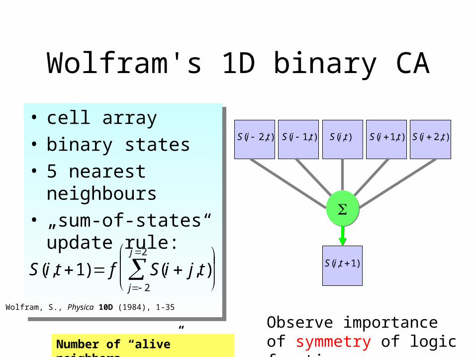
Wolfram's 1D binary CA

• cell array• binary states• 5 nearest neighbours• „sum-of-states“ update

rule:

• cell array• binary states• 5 nearest neighbours• „sum-of-states“ update

rule:

S(i, t 1) f S(i j, t)j 2

j 2

Wolfram, S., Physica 10D (1984), 1-35

S(i, t)S(i 1, t) S(i 1, t)

S(i, t 1)

S(i 2, t) S(i 2, t)

Observe importance of symmetry of logic functionNumber of “alive” neighbors

Wolfram‘s 32 „Symmetry-based“ CA rules in 5-neighborhood

S {0,1}S {0,1}

{1,2,3,4,5} {1,2,3,4,5}

S

25=32 different rules 25=32 different rulesNumber of “alive” neighbors

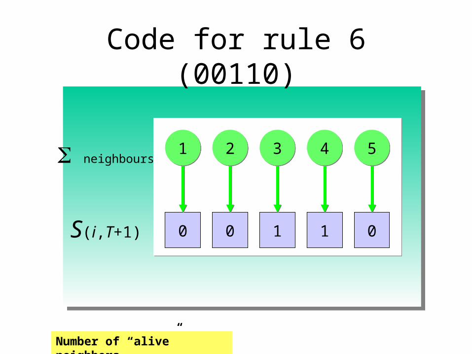
Code for rule 6 (00110)

0S(i,T+1)

neighbours11

0

22

1

33

1

44

0

55

Number of “alive” neighbors

Rule codes0 0 0 0 0

0 0 0 0 1

0 0 0 1 0

0 0 0 1 1

0 0 1 0 0

0 0 1 0 1

1 1 1 1 1

rule 0

rule 1

rule 2

rule 3

rule 4

rule 5

rule 32

Number of “alive” neighbors

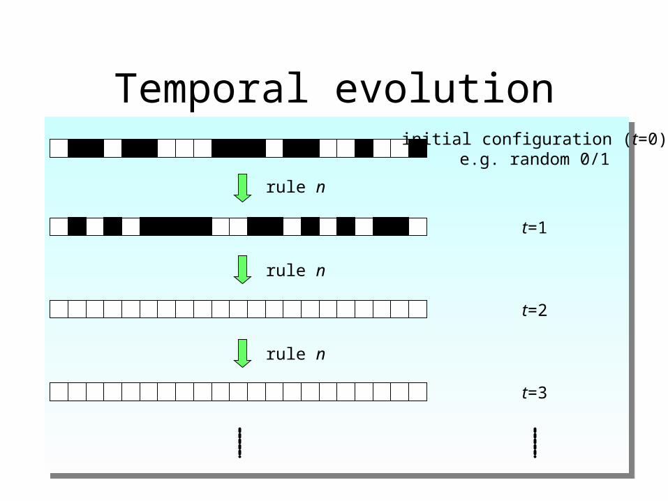
Temporal evolutioninitial configuration (t=0)

e.g. random 0/1

t=1

t=2

t=3

rule n

rule n

rule n

Temporal evolution

t=0

t=10

Rule 6: 00110

t=100

t=0

Rule 10: 01010

t=100

t=0

CA: a metaphor for morphogenesis static binary

pattern

translated into

state transition rule

rule iteration in configuration space

genotype

translation,epigenetic rules

morphogenesis of the phenotype

00 11 00 11 00

0

1

0

1

0

CA: a model for morphogenesis

update rule

iterative application of the update rule

CA state pattern

state space

genotype

epigenetic interpretation of the genotype, morphogenesis

phenotype

morphospace

CA rule mutations

11 00 0 1 0

0 1 0 1 11

swap

0 1 0 1 0

genotype phenotypedevelopmentnegate

How genotype mutations can change phenotypes?

CA rule mutations0 1 0 1 0 1 0 0 1 0

0 1 1 0 0 1 0 1 0 0 1 0 1

0 1 0 0 1 0 0 0 1

0 1 1 1 0

1 1

0 1 0 1 0 1

negate

swap

rule

Predictability?

pattern at t+t

pattern at t

explicit simulation: iterations of rule n

?hypothetical"simple algorithm" ?

How to predict a next element in sequence? Tough!

Sum of natural numbers 1… N

algorithm 1: 1+2+…+N

algorithm2: N(N+1)/2

(Gaussian formula)

Sum of natural numbers 1… N

algorithm 1: 1+2+…+N

algorithm2: N(N+1)/2

(Gaussian formula)

Predictability

n1

N

Nth prime number

algorithm 1: trial and error

algorithm2: ?no general formula

Nth prime number

algorithm 1: trial and error

algorithm2: ?no general formula

pN pn p | p / i N;i 1, p

easy Very tough!

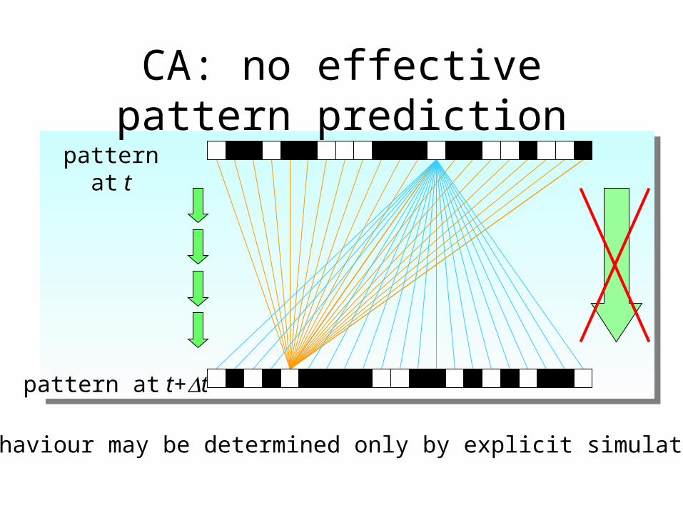
CA: no effective pattern prediction

pattern at t+t

pattern at t

behaviour may be determined only by explicit simulation

CA: deterministic, unpredictable, irreversible

• Simple rules generate complex spatio-temporal behavior

• For non-trivial rules, the spatio-temporal behaviour is computable but not predictable

• The behavior of the system is irreversible

• Similarity of rules does not imply similarity of patterns

• Simple rules generate complex spatio-temporal behavior

• For non-trivial rules, the spatio-temporal behaviour is computable but not predictable

• The behavior of the system is irreversible

• Similarity of rules does not imply similarity of patterns

Aspects of CA morphogenesisAspects of CA morphogenesis

• complex relationship between „genotype“ and „phenotype

• effects of „genes“ are not localizable in specific phenes (pleiotropy)

• phenes cannot be traced back to specific single genes (epistasisepistasis)

• phenetic effects of "mutations" are not predictable

Meinhardt, H. (1995). The Algorithmic Beauty of Sea Shells. Berlin: Springer

Patterns and morphology• Pattern: a spatially

and/or temporally ordered distribution of a physical or chemical parameter

• Pattern formation

• Form (Size and Shape)

• Morphogenesis: The spatiotemporal processes by which an organism changes is size (growth) and shape (development)

Where is the phene?

• Typification?• Comparative

measures?– length

– density

– fractal dimension

• Spatio-temporal development?

phenotype A

phenotype B