Lectures on Arithmetic Noncommutative Geometrymatilde/BookAMSULect.pdf · Lectures on Arithmetic...
145
Lectures on Arithmetic Noncommutative Geometry Matilde Marcolli
Transcript of Lectures on Arithmetic Noncommutative Geometrymatilde/BookAMSULect.pdf · Lectures on Arithmetic...
Lectures on Arithmetic
Noncommutative Geometry
Matilde Marcolli

v
And indeed there will be timeTo wonder “Do I dare?” and, “Do I dare?”Time to turn back and descend the stair.
...
Do I dareDisturb the Universe?
...
For I have known them all already, known them all;Have known the evenings, mornings, afternoons,I have measured out my life with coffee spoons.
...
I should have been a pair of ragged clawsScuttling across the floors of silent seas....No! I am not Prince Hamlet, nor was meant to be;Am an attendant lord, one that will doTo swell a progress, start a scene or two...At times, indeed, almost ridiculous–Almost, at times, the Fool....We have lingered in the chambers of the seaBy sea-girls wreathed with seaweed red and brownTill human voices wake us, and we drown.
(T.S. Eliot, “The Love Song of J. Alfred Prufrock”)

Contents
Preface ix
Chapter 1. Ouverture 11. The NCG dictionary 32. Noncommutative spaces 43. Spectral triples 64. Why noncommutative geometry? 12
Chapter 2. Noncommutative modular curves 151. Modular curves 152. The noncommutative boundary of modular curves 223. Limiting modular symbols 274. Hecke eigenforms 395. Selberg zeta function 416. The modular complex and K-theory of C∗-algebras 427. Intermezzo: Chaotic Cosmology 44
Chapter 3. Quantum statistical mechanics and Galois theory 511. Quantum Statistical Mechanics 532. The Bost–Connes system 563. Noncommutative Geometry and Hilbert’s 12th problem 614. The GL2 system 645. Quadratic fields 70
Chapter 4. Noncommutative geometry at arithmetic infinity 811. Schottky uniformization 812. Dynamics and noncommutative geometry 883. Arithmetic infinity: archimedean primes 934. Arakelov geometry and hyperbolic geometry 975. Intermezzo: Quantum gravity and black holes 1006. Dual graph and noncommutative geometry 1057. Arithmetic varieties and L–factors 1098. Archimedean cohomology 115
Chapter 5. Vistas 125
Bibliography 131
vii

Preface
Noncommutative geometry nowadays looks as a vast building site.
On the one hand, practitioners of noncommutative geometry (or ge-ometries) already built up a large and swiftly growing body of excitingmathematics, challenging traditional boundaries and subdivisions.
On the other hand, noncommutative geometry lacks common foun-dations: for many interesting constructions of “noncommutative spaces”we cannot even say for sure which of them lead to isomorphic spaces,because they are not objects of an all–embracing category (like that oflocally ringed topological spaces in commutative geometry).
Matilde Marcolli’s lectures reflect this spirit of creative growth andinterdisciplinary research.
She starts Chapter 1 with a sketch of philosophy of noncommuta-tive geometry a la Alain Connes. Briefly, Connes suggests imaginingC∗–algebras as coordinate rings. He then supplies several bridges tocommutative geometry by his construction of “bad quotients” of com-mutative spaces via crossed products and his treatment of noncom-mutative Riemannian geometry. Finally, algebraic tools like K–theoryand cyclic cohomology serve to further enhance geometric intuition.
Marcolli then proceeds to explaining some recent developmentsdrawing upon her recent work with several collaborators. A commonthread in all of them is the study of various aspects of uniformization:classical modular group, Schottky groups. The modular group actsupon the complex half plane, partially compactified by cusps: rationalpoints of the boundary projective line. The action becomes “bad” atirrational points, and here is where noncommutative geometry entersthe game. A wealth of classical number theory is encoded in the co-efficients of modular forms, their Mellin transforms, Hecke operatorsand modular symbols. Their counterparts living at the noncommuta-tive boundary have only recently started to unravel themselves, andMarcolli gives a beautiful overview of what is already understood inChapters 2 and 3.
ix
x PREFACE
Schottky uniformization provides a visualization of Arakelov’s ge-ometry at arithmetic infinity, which serves as the main motivation ofChapter 4.
Among the most tantalizing developments is the recurrent emer-gence of patches of common ground for number theory and theoreticalphysics.
In fact, one can present in this light the famous theorem of youngGauss characterising regular polygons that can be constructed usingonly ruler and compass. In his Tagebuch entry of March 30 he an-nounced that a regular 17–gon has this property.
Somewhat modernizing his discovery, one can present it in the fol-lowing way.
In the complex plane, roots of unity of degree n form vertices ofa regular n–gone. Hence it makes sense to imagine that we studythe ruler and compass constructions as well not in the Euclidean, butin the complex plane. This has an unexpected consequence: we cancharacterize the set of all points constructible in this way as the maxi-mal Galois 2–extension of Q. It remains to calculate the Galois groupof Q(e2πi/17): since it is cyclic of order 16, this root of unity is con-structible. Moreover, the same is true for all p–gons where p is a primeof the form 2n + 1 but not for other primes.
A remarkable feature of this result is the appearance of a hiddensymmetry group. In fact, the definitions of a regular n–gon and rulerand compass constructions are initially formulated in terms of Eu-clidean plane geometry and suggest that the relevant symmetry groupmust be that of rigid rotations SO (2), eventually extended by reflec-tions and shifts. This conclusion turns out to be totally misleading: in-stead, one should rely upon Gal (Q/Q). The action of the latter groupupon roots of unity of degree n factors through the maximal abelianquotient and is given by ζ 7→ ζk, with k running over all k mod nwith (k, n) = 1, whereas the action of the rotation group is given byζ 7→ ζ0ζ with ζ0 running over all n–th roots. Thus, the Gal (Q/Q)–symmetry does not conserve angles between vertices which seem to bebasic for the initial problem. Instead, it is compatible with additionand multiplication of complex numbers, and this property proves to becrucial.
With some stretch of imagination, one can recognize in the Eu-clidean avatar of this picture a physics flavor (putting it somewhatpompously, it appeals to the kinematics of 2–dimensional rigid bodies
PREFACE xi
in gravitational vacuum), whereas the Galois avatar definitely belongsto number theory.
In the Marcolli lectures, stressing number theory, physics themespop up at the end of Chapter 2 (Chaotic Cosmology in general rela-tivity), the beginning of Chapter 3 (formalism of quantum statisticalmechanics), and finally, sec. 5 of Chapter 4 where some models ofblack holes in general relativity turn out to have the same mathe-matical description as ∞–adic fibers of curves in Arakelov geometry.The reemergence of Gauss’ Galois group Galab (Q/Q) in Bost–Connessymmetry breaking, and of Gauss’ statistics of continued fractions inthe Chaotic Cosmology models, shows that connections with classicalmathematics are as strong as ever.
Hopefully, this lively exposition will attract young researchers andincite them to engage themselves in exploration of the rich new terri-tory.
Yuri I. Manin. Bonn, March 17, 2005.
CHAPTER 1
Ouverture
Noncommutative geometry, as developed by Connes starting in theearly ’80s ([16], [18], [21]), extends the tools of ordinary geometry totreat spaces that are quotients, for which the usual “ring of functions”,defined as functions invariant with respect to the equivalence relation,is too small to capture the information on the “inner structure” ofpoints in the quotient space. Typically, for such spaces functions on thequotients are just constants, while a nontrivial ring of functions, whichremembers the structure of the equivalence relation, can be definedusing a noncommutative algebra of coordinates, analogous to the non-commuting variables of quantum mechanics. These “quantum spaces”are defined by extending the Gel’fand–Naimark correspondence
X loc.comp. Hausdorff space⇔ C0(X) abelian C∗-algebra
by dropping the commutativity hypothesis in the right hand side. Thecorrespondence then becomes a definition of what is on the left handside: a noncommutative space.
Such quotients are abundant in nature. They arise, for instance,from foliations. Several recent results also show that noncommuta-tive spaces arise naturally in number theory and arithmetic geometry.The first instance of such connections between noncommutative geom-etry and number theory emerged in the work of Bost and Connes [9],which exhibits a very interesting noncommutative space with remark-able arithmetic properties related to class field theory. This reveals avery useful dictionary that relates the phenomena of spontaneous sym-metry breaking in quantum statistical mechanics to the mathematics ofGalois theory. This space can be viewed as the space of 1-dimensionalQ-lattices up to scale, modulo the equivalence relation of commensu-rability (cf. [32]). This space is closely related to the noncommutativespace used by Connes to obtain a spectral realization of the zeros of theRiemann zeta function, [23]. In fact, this is again the space of com-mensurability classes of 1-dimensional Q-lattices, but with the scalefactor also taken into account.
More recently, other results that point to deep connections betweennoncommutative geometry and number theory appeared in the work
1
2 1. OUVERTURE
of Connes and Moscovici [41] [42] on the modular Hecke algebras.This shows that the Rankin–Cohen brackets, an important algebraicstructure on modular forms [110], have a natural interpretation in thelanguage of noncommutative geometry, in terms of the Hopf algebra ofthe transverse geometry of codimension one foliations. The modularHecke algebras, which naturally combine products and action of Heckeoperators on modular forms, can be viewed as the “holomorphic part”of the algebra of coordinates on the space of commensurability classesof 2-dimensional Q-lattices constructed in joint work of Connes andthe author [32].
Cases of occurrences of interesting number theory within noncom-mutative geometry can be found in the classification of noncommuta-tive three-spheres by Connes and Dubois–Violette [28] [29]. Here thecorresponding moduli space has a ramified cover by a noncommutativenilmanifold, where the noncommutative analog of the Jacobian of thiscovering map is expressed naturally in terms of the ninth power of theDedekind eta function. Another such case occurs in Connes’ calcula-tion [25] of the explicit cyclic cohomology Chern character of a spectraltriple on SUq(2) defined by Chakraborty and Pal [13].
Other instances of noncommutative spaces that arise in the contextof number theory and arithmetic geometry can be found in the non-commutative compactification of modular curves of [26], [83]. Thisnoncommutative space is again related to the noncommutative geom-etry of Q-lattices. In fact, it can be seen as a stratum in the com-pactification of the space of commensurability classes of 2-dimensionalQ-lattices (cf. [32]).
Another context in which noncommutative geometry provides a use-ful tool for arithmetic geometry is in the description of the totallydegenerate fibers at “arithmetic infinity” of arithmetic varieties overnumber fields, analyzed in joint work of the author with Katia Consani([44], [45], [46], [47]).
The present text is based on a series of lectures given by the authorat Vanderbilt University in May 2004, as well as on previous series oflectures given at the Fields Institute in Toronto (2002), at the Univer-sity of Nottingham (2003), and at CIRM in Luminy (2004).
The main focus of the lectures is the noncommutative geometryof modular curves (following [83]) and of the archimedean fibers ofarithmetic varieties (following [44]). A chapter on the noncommutativespace of commensurability classes of 2-dimensional Q-lattices is alsoincluded (following [32]). The text reflects very closely the style ofthe lectures. In particular, we have tried more to convey the generalpicture than the details of the proofs of the specific results. Though
1. THE NCG DICTIONARY 3
many proofs have not been included in the text, the reader will findreferences to the relevant literature, where complete proofs are provided(in particular [32], [44], [38], and [83]).
More explicitly, the text is organized as follows:
• We start by recalling a few preliminary notions of noncommu-tative geometry (following [21]).• The second chapter describes how various arithmetic proper-
ties of modular curves can be seen by their “noncommutativeboundary”. This part is based on the joint work of Yuri Maninand the author. The main references are [83], [84], [85].• The third chapter includes an account of the work of Connes
and the author [32] on the noncommutative geometry of com-mensurability classes of Q-lattices. It also includes a discussionof the relation of the noncommutative space of commensura-bility classes of Q-lattices to the Hilbert 12th problem of ex-plicit class field theory and a section on the results of Connes,Ramachandran and the author [38] on the construction of aquantum statistical mechnical system that fully recovers theexplicit class field theory of imaginary quadratic fields. Wealso included a brief discussion of Manin’s real multiplicationprogram [75] [76] and the problem of real quadratic fields.• The noncommutative geometry of the fibers at “arithmetic
infinity” of varieties over number fields is the content of theremaining chapter, based on joint work of Consani and theauthor, for which the references are [44], [45], [46], [47], [48].This chapter also contains a detailed account of Manin’s for-mula for the Green function of Arakelov geometry for arith-metic surfaces, based on [79], and a proposed physical inter-pretation of this formula, as in [82].
1. The NCG dictionary
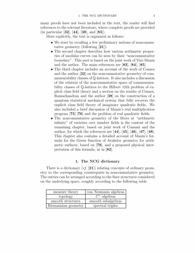
There is a dictionary (cf. [21]) relating concepts of ordinary geom-etry to the corresponding counterparts in noncommutative geometry.The entries can be arranged according to the finer structures consideredon the underlying space, roughly according to the following table.
measure theory von Neumann algebrastopology C∗–algebras
smooth structures smooth subalgebrasRiemannian geometry spectral triples
4 1. OUVERTURE
It is important to notice that, usually, the notions of noncommuta-tive geometry are “richer” than the corresponding entries of the dictio-nary on the commutative side. For instance, as Connes discovered, non-commutative measure spaces (von Neumann algebras) come endowedwith a natural time evolution which is trivial in the commutative case.Similarly, at the level of topology one often sees phenomena that arecloser to rigid analytic geometry. This is the case, for instance, with thenoncommutative tori Tθ, which already at the C∗-algebra level exhibitmoduli that behave much like moduli of one-dimensional complex tori(elliptic curves) in the commutative case.
In the context we are going to discuss this richer structure of non-commutative spaces is crucial, as it permits us to use tools like C∗-algebras (topology) to study the properties of more rigid spaces likealgebraic or arithmetic varieties.
2. Noncommutative spaces
The way to assign the algebra of coordinates to a quotient spaceX = Y/ ∼ can be explained in a short slogan as follows:
• Functions on Y with f(a) = f(b) for a ∼ b. Poor!
• Functions fab on the graph of the equivalence relation. Good!
The second description leads to a noncommutative algebra, as theproduct, determined by the groupoid law of the equivalence relation,has the form of a convolution product (like the product of matrices).
For sufficiently nice quotients, even though the two notions arenot the same, they are related by Morita equivalence, which is thesuitable notion of “isomorphism” between noncommutative spaces. Formore general quotients, however, the two notions truly differ and thesecond one is the only one that allows one to continue to make senseof geometry on the quotient space.
A very simple example illustrating the above situation is the fol-lowing (cf. [24]). Consider the topological space Y = [0, 1] × 0, 1with the equivalence relation (x, 0) ∼ (x, 1) for x ∈ (0, 1). By the firstmethod one only obtains constant functions C, while by the secondmethod one obtains
f ∈ C([0, 1])⊗M2(C) : f(0) and f(1) diagonal which is an interesting nontrivial algebra.
The idea of preserving the information on the structure of the equiv-alence relation in the description of quotient spaces has analogs inGrothendieck’s theory of stacks in algebraic geometry.
2. NONCOMMUTATIVE SPACES 5
2.1. Morita equivalence. In noncommutative geometry, isomor-phisms of C∗-algebras are too restrictive to provide a good notion ofisomorphisms of noncommutative spaces. The correct notion is pro-vided by Morita equivalence of C∗-algebras.
We have equivalent C∗-algebras A1 ∼ A2 if there exists a bimoduleM, which is a right HilbertA1 module with anA1-valued inner product〈·, ·〉A1, and a left Hilbert A2-module with an A2-valued inner product〈·, ·〉A2, such that we have:
• We obtain all Ai as the closure of the span of
〈ξ1, ξ2〉Ai: ξ1, ξ2 ∈ M.
• ∀ξ1, ξ2, ξ3 ∈ M we have
〈ξ1, ξ2〉A1ξ3 = ξ1〈ξ2, ξ3〉A2 .
• A1 and A2 act onM by bounded operators,
〈a2ξ, a2ξ〉A1 ≤ ‖a2‖2〈ξ, ξ〉A1 〈a1ξ, a1ξ〉A2 ≤ ‖a1‖2〈ξ, ξ〉A2
for all a1 ∈ A1, a2 ∈ A2, ξ ∈ M.
This notion of equivalence roughly means that one can transfermodules back and forth between the two algebras.
2.2. The tools of noncommutative geometry. Once one iden-tifies in a specific problem a space that, by its nature of quotient of thetype described above, is best described as a noncommutative space,there is a large set of well developed techniques that one can use tocompute invariants and extract essential information from the geome-try. The following is a list of some such techniques, some of which willmake their appearance in the cases treated in these notes.
• Topological invariants: K-theory• Hochschild and cyclic cohomology• Homotopy quotients, assembly map (Baum-Connes)• Metric structure: Dirac operator, spectral triples• Characteristic classes, zeta functions
We will recall the necessary notions when needed. We now beginby taking a closer look at the analog in the noncommutative world ofRiemannian geometry, which is provided by Connes’ notion of spectraltriples.
6 1. OUVERTURE
3. Spectral triples
Spectral triples are a crucial notion in noncommutative geometry.They provide a powerful and flexible generalization of the classicalstructure of a Riemannian manifold. The two notions agree on a com-mutative space. In the usual context of Riemannian geometry, thedefinition of the infinitesimal element ds on a smooth spin manifoldcan be expressed in terms of the inverse of the classical Dirac opera-tor D. This is the key remark that motivates the theory of spectraltriples. In particular, the geodesic distance between two points on themanifold is defined in terms of D−1 (cf. [21] §VI). The spectral triple(A, H, D) that describes a classical Riemannian spin manifold is givenby the algebra A of complex valued smooth functions on the manifold,the Hilbert space H of square integrable spinor sections, and the clas-sical Dirac operator D. These data determine completely and uniquelythe Riemannian geometry on the manifold. It turns out that, whenexpressed in this form, the notion of spectral triple extends to moregeneral non-commutative spaces, where the data (A, H, D) consist ofa C∗-algebra A (or more generally of some smooth subalgebra of a C∗-algebra) with a representation in the algebra of bounded operators ona separable Hilbert space H, and an operator D on H that verifies themain properties of a Dirac operator.
We recall the basic setting of Connes’ theory of spectral triples. Fora more complete treatment see [21], [22], [39].
Definition 3.1. A spectral triple (A,H, D) consists of a C∗-algebraA with a representation
ρ : A → B(H)
in the algebra of bounded operators on a separable Hilbert space H, andan operator D (called the Dirac operator) on H, which satisfies thefollowing properties:
(1) D is self-adjoint.(2) For all λ /∈ R, the resolvent (D − λ)−1 is a compact operator
on H.(3) The commutator [D, ρ(a)] is a bounded operator on H, for all
a ∈ A0 ⊂ A, a dense involutive subalgebra of A.
The property (2) of Definition 3.1 can be regarded as a general-ization of the ellipticity property of the standard Dirac operator on acompact manifold. In the case of ordinary manifolds, we can consideras subalgebra A0 the algebra of smooth functions, as a subalgebra ofthe commutative C∗-algebra of continuous functions. In fact, in the
3. SPECTRAL TRIPLES 7
classical case of Riemannian manifolds, property (3) is equivalent theLipschitz condition, hence it is satisfied by a larger class than that ofsmooth functions.
Thus, the basic geometric structure encoded by the theory of spec-tral triples is Riemannian geometry, but in more refined cases, suchas Kahler geometry, the additional structure can be easily encoded asadditional symmetries. We will see, for instance, a case (cf. [44] [48])where the algebra involves the action of the Lefschetz operator of acompact Kahler manifold, hence it encodes the information (at thecohomological level) on the Kahler form.
Since we are mostly interested in the relations between noncom-mutative geometry and arithmetic geometry and number theory, anespecially interesting feature of spectral triples is that they have anassociated family of zeta functions and a theory of volumes and inte-gration, which is related to special values of these zeta functions. (Thefollowing treatment is based on [21], [22].)
3.1. Volume form. A spectral triple (A,H, D) is said to be ofdimension n, or n–summable if the operator |D|−n is an infinitesimalof order one, which means that the eigenvalues λk(|D|−n) satisfy theestimate λk(|D|−n) = O(k−1).
For a positive compact operator T such that
k−1∑
j=0
λj(T ) = O(log k),
the Dixmier trace Trω(T ) is the coefficient of this logarithmic diver-gence, namely
(1.1) Trω(T ) = limω
1
log k
k∑
j=1
λj(T ).
Here the notation limω takes into account the fact that the sequence
S(k, T ) :=1
log k
k∑
j=1
λj(T )
is bounded though possibly non-convergent. For this reason, the usualnotion of limit is replaced by a choice of a linear form limω on theset of bounded sequences satisfying suitable conditions that extendanalogous properties of the limit. When the sequence S(k, T ) converges(1.1) is just the ordinary limit Trω(T ) = limk→∞ S(k, T ). So defined,the Dixmier trace (1.1) extends to any compact operator that is aninfinitesimal of order one, since any such operator is the difference of
8 1. OUVERTURE
two positive ones. The operators for which the Dixmier trace doesnot depend on the choice of the linear form limω are called measurableoperators.
On a non-commutative space the operator |D|−n generalizes thenotion of a volume form. The volume is defined as
(1.2) V = Trω(|D|−n).
More generally, consider the algebra A generated by A and [D,A].Then, for a ∈ A, integration with respect to the volume form |D|−n isdefined as
(1.3)
∫a :=
1
VTrω(a|D|−n).
The usual notion of integration on a Riemannian spin manifold Mcan be recovered in this context (cf. [21], [70]) through the formula (neven): ∫
M
fdv =(2n−[n/2]−1πn/2nΓ(n/2)
)Trω(f |D|−n).
Here D is the classical Dirac operator on M associated to the metricthat determines the volume form dv, and f in the right hand side isregarded as the multiplication operator acting on the Hilbert space ofsquare integrable spinors on M .
3.2. Zeta functions. An important function associated to theDirac operator D of a spectral triple (A,H, D) is its zeta function
(1.4) ζD(z) := Tr(|D|−z) =∑
λ
Tr(Π(λ, |D|))λ−z,
where Π(λ, |D|) denotes the orthogonal projection on the eigenspaceE(λ, |D|).
An important result in the theory of spectral triples ([21] §IVProposition 4) relates the volume (1.2) with the residue of the zetafunction (1.4) at s = 1 through the formula
(1.5) V = lims→1+
(s− 1)ζD(s) = Ress=1Tr(|D|−s).
There is a family of zeta functions associated to a spectral triple(A,H, D), to which (1.4) belongs. For an operator a ∈ A, we candefine the zeta functions
(1.6) ζa,D(z) := Tr(a|D|−z) =∑
λ
Tr(a Π(λ, |D|))λ−z
3. SPECTRAL TRIPLES 9
and
(1.7) ζa,D(s, z) :=∑
λ
Tr(a Π(λ, |D|))(s− λ)−z.
These zeta functions are related to the heat kernel e−t|D| by Mellintransform
(1.8) ζa,D(z) =1
Γ(z)
∫ ∞
0
tz−1Tr(a e−t|D|) dt
where
(1.9) Tr(a e−t|D|) =∑
λ
Tr(a Π(λ, |D|))e−tλ =: θa,D(t).
Similarly,
(1.10) ζa,D(s, z) =1
Γ(z)
∫ ∞
0
θa,D,s(t) tz−1 dt
with
(1.11) θa,D,s(t) :=∑
λ
Tr(a Π(λ, |D|))e(s−λ)t.
Under suitable hypothesis on the asymptotic expansion of (1.11) (cf.Theorem 2.7-2.8 of [78] §2), the functions (1.6) and (1.7) admit aunique analytic continuation (cf. [39]) and there is an associated reg-ularized determinant in the sense of Ray–Singer (cf. [100]):
(1.12) det∞ a,D
(s) := exp
(− d
dzζa,D(s, z)|z=0
).
The family of zeta functions (1.6) also provides a refined notion ofdimension for a spectral triple (A,H, D), called the dimension spec-trum. This is a subset Σ = Σ(A,H, D) in C with the property that
all the zeta functions (1.6), as a varies in A, extend holomorphicallyto C \ Σ.
Examples of spectral triples with dimension spectrum not containedin the real line can be constructed out of Cantor sets.
3.3. Index map. The data of a spectral triple determine an indexmap. In fact, the self-adjoint operator D has a polar decomposition,D = F |D|, where |D| =
√D2 is a positive operator and F is a sign
operator, i.e. F 2 = I. Following [21] and [22] one defines a cycliccocycle
(1.13) τ(a0, a1, . . . , an) = Tr(a0[F, a1] · · · [F, an]),
where n is the dimension of the spectral triple. For n even Tr shouldbe replaced by a super trace, as usual in index theory. This cocycle
10 1. OUVERTURE
pairs with the K-groups of the algebra A (with K0 in the even case andwith K1 in the odd case), and defines a class τ in the cyclic cohomologyHCn(A) of A. The class τ is called the Chern character of the spectraltriple (A,H, D).
In the case when the spectral triple (A,H, D) has discrete dimen-sion spectrum Σ, there is a local formula for the cyclic cohomologyChern character (1.13), analogous to the local formula for the indexin the commutative case. This is obtained by producing Hochschildrepresentatives (cf. [22], [39])
(1.14) ϕ(a0, a1, . . . , an) = Trω(a0[D, a1] · · · [D, an] |D|−n).
3.4. Infinite dimensional geometries. The main difficulty inconstructing specific examples of spectral triples is to produce an op-erator D that at the same time has bounded commutators with theelements of A and produces a non-trivial index map.
It sometimes happens that a noncommutative space does not admita finitely summable spectral triple, namely one such that the operator|D|−p is of trace class for some p > 0. Obstructions to the existence ofsuch spectral triples are analyzed in [20]. It is then useful to considera weaker notion, namely that of θ-summable spectral triples. Thesehave the property that the Dirac operator satisfies
(1.15) Tr(e−tD2
) <∞ ∀t > 0.
Such spectral triples should be thought of as “infinite dimensional non-commutative geometries”.
We’ll see examples of spectral triples that are θ-summable but notfinitely summable, because of the growth rate of the multiplicities ofeigenvalues.
3.5. Spectral triples and Morita equivalences. If (A1,H, D)is a spectral triple, and we have a Morita equivalence A1 ∼ A2 im-plemented by a bimodule M which is a finite projective right Hilbertmodule over A1, then we can transfer the spectral triple from A1 toA2.
First consider the A1-bimodule Ω1D generated by
a1[D, b1] : a1, b1 ∈ A1.We define a connection
∇ :M→M⊗A1 Ω1D
by requiring that
∇(ξa1) = (∇ξ)a1 + ξ ⊗ [D, a1],
3. SPECTRAL TRIPLES 11
∀ξ ∈ M, ∀a1 ∈ A1 and ∀ξ1, ξ2 ∈ M. We also require that
〈ξ1,∇ξ2〉A1 − 〈∇ξ1, ξ2〉A1 = [D, 〈ξ1, ξ2〉A1 ].
This induces a spectral triple (A2, H, D) obtained as follows.The Hilbert space is given by H =M⊗A1 H. The action takes the
forma2 (ξ ⊗A1 x) := (a2ξ)⊗A1 x.
The Dirac operator is given by
D(ξ ⊗ x) = ξ ⊗D(x) + (∇ξ)x.
Notice that we need a Hermitian connection ∇, because commuta-tors [D, a] for a ∈ A1 are non-trivial, hence 1 ⊗ D would not be well
defined on H.
3.6. K-theory of C∗-algebras. The K-groups are important in-variants of C∗-algebras that capture information on the topology ofnon-commutative spaces, much like cohomology (or more appropriatelytopological K-theory) captures information on the topology of ordinaryspaces. For a C∗-algebra A, we have:
3.6.1. K0(A). This group is obtained by considering idempotents(p2 = p) in matrix algebras over A. Notice that, for a C∗-algebra, itis sufficient to consider projections (P 2 = P , P = P ∗). In fact, wecan always replace an idempotent p by a projection P = pp∗(1− (p−p∗)2)−1, preserving the von Neumann equivalence. Then we considerP ' Q if and only if P = X∗X, Q = XX∗, for X = partial isometry(X = XX∗X), and we impose the stable equivalence: P ∼ Q, forP ∈ Mn(A) and Q ∈ Mm(A), if and only if there exists R a projectionwith P⊕R ' Q⊕R. We define K0(A)+ to be the monoid of projectionsmodulo these equivalences and we let K0(A) be its Grothendieck group.
3.6.2. K1(A). Consider the group GLn(A) of invertible elementsin the matrix algebraMn(A), and GL0
n(A) the identity component ofGLn(A). The morphism
GLn(A)→ GLn+1(A) a 7→(
a 00 1
)
inducesGLn(A)/GL0
n(A)→ GLn+1(A)/GL0n+1(A).
The group K1(A) is defined as the direct limit of these morphisms.Notice that K1(A) is abelian even if the GLn(A)/GL0
n(A) are not.
In general, K-theory is not easy to compute. This has led to twofundamental developments in noncommutative geometry. The first iscyclic cohomology (cf. [18], [19], [21]), introduced by Connes in 1981,
12 1. OUVERTURE
which provides cycles that pair with K-theory, and a Chern charac-ter. The second development is the geometrically defined K-theory ofBaum–Connes [7] and the assembly map
(1.16) µ : K∗(X, G)→ K∗(C0(X) o G)
from the geometric to the analytic K-theory. Much work has gone, inrecent years, into exploring the range of validity of the Baum–Connesconjecture, according to which the assembly map gives an isomorphismbetween these two different notions of K-theory.
4. Why noncommutative geometry?
In this short introductory section about noncommutative geometrywe have tried to stress the idea that this version of geometry allows oneto progress beyond the limits of applicability of ordinary “classical”geometry. Typically, this is the type of situation that presents itselfat the boundary of classically defined objects, where certain quotientsbecome ill behaved from the point of view of classical geometry. Insuch cases, by viewing the resulting spaces as noncommutative, whichmeans working with a noncommutative algebra of coordinates replacingthe usual commutative ring of functions of a space, one can continueto apply the tools and results of ordinary geometry.
Hopefully, this constitutes a convincing explanation of why one isled naturally to consider this type of geometry in a variety of contextsthat have to do with boundary strata of certain classical objects andin general with equivalence relations that stem from suitably enlargingthe class of objects to include some degenerate cases (all this seemsquite vague at this point, but much of the content of the followingchapters will be concrete illustrations of this principle).
Still, it is probably a good idea to spend a few more words in jus-tifying the use of noncommutative geometry specifically in the contextof Number Theory and Arithmetic Algebraic Geometry, and what oneexpects from this new set of tools.
There are at present several directions in which the use of toolsof noncommuative geometry in number theory may lead to interestingprogress. One is the explicit class field theory problem. In this case,the results of Bost–Connes [9] showed that the Galois theory of thecyclotomic field Qab lives naturally as symmetries of zero temperatureequilibrium states of a quantum statistical mechanical system. Recentwork of Connes and the author showed that a similar noncommutativespace with a natural time evolution gives rise to zero temperature equi-librium states whose symmetries are given by the automorphisms of themodular field. In joint work with Ramachandran, we showed how these
4. WHY NONCOMMUTATIVE GEOMETRY? 13
constructions fit into a possible theory of noncommutative Shimura va-rieties, and we exhibited a related quantum statistical mechanical sys-tem that recovers the explicit class field theory for imaginary quadraticfields. This opens up a very concrete possibility that noncommutativegeometry may be able to say something new about the real quadraticfields or other cases where the Hilbert 12th problem of explicit classfield theory is not yet fully understood from a purely number theoreticviewpoint. Suggestive connections between the problem for real qua-dratic fields and noncommutative geometry were discussed by Maninin [75] and [76]. These results and perspectives are described in achapter of this volume.
Another direction in which noncommutative geometry may be ableto yield new results in number theory and arithmetic geometry is re-lated to L-functions. This possibility was first brought to light byConnes’ work on the spectral realization of the zeros of the Riemannzeta function and of L-functions with Grossencharakter [23]. His workprovided a new approach to the generalized Riemann hypothesis througha Selberg trace formula for the action of the idele class group on anoncommutative space obtained as a quotient (viewed in the sensediscussed in this section) of the space of adeles. The noncommutativespace involved in this construction is closely related (up to a duality) tothe one of the Bost–Connes system. In a different direction, the recentwork of Consani and the author showed that noncommutative tech-niques may help in describing the geometry of the fibers at infinity ofarithmetic varieties and the correspnding Gamma factors contributingto the L-function. The latter results are described in the last chapterof this volume. There is reason to be optimistic that a combinationof these approaches will lead to some new results about L-functions ofarithmetic varieties.
Sometime noncommutative geometry leads to new conceptual ex-planations and points of view on classical number theoretic objects. Astriking example is given by the modular Hecke algebras of Connes andMoscovici [41] [42] that recover and extend structures like the Rankin–Cohen brackets of modular forms [110] in terms of Hopf algebra sym-metries of noncommutative spaces and their Hopf cyclic cohomology.In a similar spirit, the results of Manin and the author discussed inthe first chapter of this volume, recover arithmetic properties of mod-ular curves from a noncommutative boundary, opening the possibilityof similar constructions on the boundary of other moduli spaces ofarithmetic significance.
14 1. OUVERTURE
For the purpose of this monograph, we have made a selection ofsome recent results illustrating the interactions between noncommuta-tive geometry and number theory/arithmetic geometry, reflecting somecontributions of the author. In general, the subject is still a large“building site” in rapid evolution, but enough results have emergedso far to make the underlying vision look increasingly promising. Atleast, it seems to be a good time to start collecting the results and theperspectives they open and present them in a unified picture, whichwill outline the shape of the emerging landscape of what we may call“arithmetic noncommutative geometry”. We hope that this book willsucceed, at least in part, in this goal.
An acknowledgment. Many thanks are due to Alain Connes,Katia Consani, Yuri Manin, and Niranjan Ramachandran, whose con-tribution and insight gave so much to the work described in this mono-graph. I especially thank Yuri Manin for contributing a nice prefaceto this volume. I thank the universities of Toronto, Nottingham, andVanderbilt for creating the occasion for the lecture series out of whichthis volume evolved. I thank Arthur Greenspoon for a careful proof-reading of the manuscript. I also thank Ed Dunne for encouraging meto write all this in book form for the AMS.
CHAPTER 2
Noncommutative modular curves
The results of this section are mostly based on the joint work ofYuri Manin and the author [83], with additional material from [84]and [85]. We include necessary preliminary notions on modular curvesand on noncommutative tori, respectively based on the papers [81] and[16], [101].
We first recall some aspects of the classical theory of modularcurves. We will then show that these notions can be entirely recoveredand enriched through the analysis of a noncommutative space associ-ated to a compactification of modular curves, which includes noncom-mutative tori as possible degenerations of elliptic curves.
1. Modular curves
Let G be a finite index subgroup of the modular group Γ = PSL(2, Z),and let XG denote the quotient
(2.1) XG := G\H2
where H2 is the 2-dimensional real hyperbolic plane, namely the upperhalf plane z ∈ C : =z > 0 with the metric ds2 = |dz|2/(=z)2.Equivalently, we identify H2 with the Poincare disk z : |z| < 1 withthe metric ds2 = 4|dz|2/(1− |z|2)2.
We denote the quotient map by φ : H2 → XG.Let P denote the coset space P := Γ/G. We can write the quotient
XG equivalently as
XG = Γ\(H2 × P).
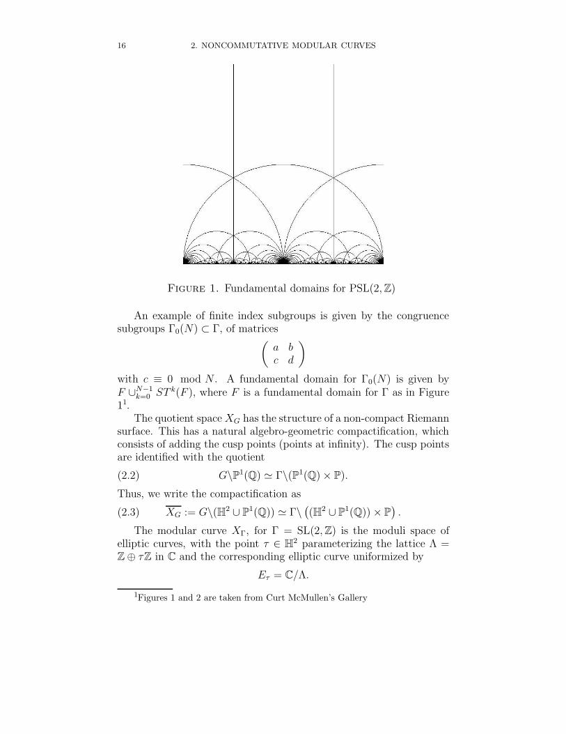
A tessellation of the hyperbolic plane H2 by fundamental domainsfor the action of PSL(2, Z) is illustrated in Figure 1. The action ofPSL(2, Z) by fractional linear transformations z 7→ az+b
cz+dis usually
written in terms of the generators S : z 7→ −1/z and T : z 7→ z + 1(inversion and translation). Equivalently, PSL(2, Z) can be identifiedwith the free product PSL(2, Z) ∼= Z/2 ∗ Z/3, with generators σ, τ oforder two and three, respectively given by σ = S and τ = ST .
15
16 2. NONCOMMUTATIVE MODULAR CURVES
Figure 1. Fundamental domains for PSL(2, Z)
An example of finite index subgroups is given by the congruencesubgroups Γ0(N) ⊂ Γ, of matrices
(a bc d
)
with c ≡ 0 mod N . A fundamental domain for Γ0(N) is given byF ∪N−1
k=0 ST k(F ), where F is a fundamental domain for Γ as in Figure11.
The quotient space XG has the structure of a non-compact Riemannsurface. This has a natural algebro-geometric compactification, whichconsists of adding the cusp points (points at infinity). The cusp pointsare identified with the quotient
(2.2) G\P1(Q) ' Γ\(P1(Q)× P).
Thus, we write the compactification as
(2.3) XG := G\(H2 ∪ P1(Q)) ' Γ\((H2 ∪ P1(Q))× P
).
The modular curve XΓ, for Γ = SL(2, Z) is the moduli space ofelliptic curves, with the point τ ∈ H2 parameterizing the lattice Λ =Z⊕ τZ in C and the corresponding elliptic curve uniformized by
Eτ = C/Λ.
1Figures 1 and 2 are taken from Curt McMullen’s Gallery
1. MODULAR CURVES 17
The unique cusp point corresponds to the degeneration of the ellipticcurve to the cylinder C∗, when τ →∞ in the upper half plane.
The other modular curves, obtained as quotients XG by a con-gruence subgroup, can also be interpreted as moduli spaces: they aremoduli spaces of elliptic curves with level structure. Namely, for ellip-tic curves E = C/Λ, this is an additional information on the torsionpoints 1
NΛ/Λ ⊂ QΛ/Λ of some level N .
For instance, in the case of the principal congruence subgroupsΓ(N) of matrices
M =
(a bc d
)∈ Γ
such that M ≡ Id mod N , points in the modular curve Γ(N)\H2
classify elliptic curves Eτ = C/Λ, with Λ = Z + Zτ , together witha basis 1/N, τ/N for the torsion subgroup 1
NΛ/Λ. The projection
XΓ(N) → XΓ forgets the extra structure.In the case of the groups Γ0(N), points in the quotient Γ0(N)\H2
classify elliptic curves together with a cyclic subgroup of Eτ of orderN . This extra information is equivalent to an isogeny φ : Eτ → Eτ ′
where the cyclic group is Ker(φ). Recall that an isogeny is a morphismφ : Eτ → Eτ ′ such that φ(0) = 0. These are implemented by the actionof GL+
2 (Q) on H2, namely Eτ and Eτ ′ are isogenous if and only if τand τ ′ in H2 are in the same orbit of GL+
2 (Q).
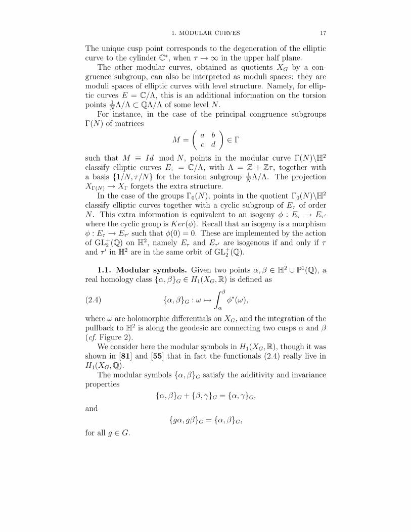
1.1. Modular symbols. Given two points α, β ∈ H2 ∪ P1(Q), areal homology class α, βG ∈ H1(XG, R) is defined as
(2.4) α, βG : ω 7→∫ β
α
φ∗(ω),
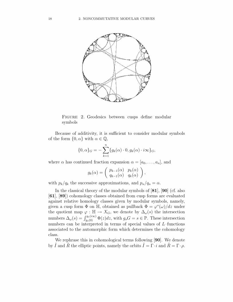
where ω are holomorphic differentials on XG, and the integration of thepullback to H2 is along the geodesic arc connecting two cusps α and β(cf. Figure 2).
We consider here the modular symbols in H1(XG, R), though it wasshown in [81] and [55] that in fact the functionals (2.4) really live inH1(XG, Q).
The modular symbols α, βG satisfy the additivity and invarianceproperties
α, βG + β, γG = α, γG,
and
gα, gβG = α, βG,
for all g ∈ G.
18 2. NONCOMMUTATIVE MODULAR CURVES
Figure 2. Geodesics between cusps define modularsymbols
Because of additivity, it is sufficient to consider modular symbolsof the form 0, α with α ∈ Q,
0, αG = −n∑
k=1
gk(α) · 0, gk(α) · i∞G,
where α has continued fraction expansion α = [a0, . . . , an], and
gk(α) =
(pk−1(α) pk(α)qk−1(α) qk(α)
),
with pk/qk the successive approximations, and pn/qn = α.
In the classical theory of the modular symbols of [81], [90] (cf. also[61], [89]) cohomology classes obtained from cusp forms are evaluatedagainst relative homology classes given by modular symbols, namely,given a cusp form Φ on H, obtained as pullback Φ = ϕ∗(ω)/dz underthe quotient map ϕ : H → XG, we denote by ∆ω(s) the intersection
numbers ∆ω(s) =∫ gs(i∞)
gs(0)Φ(z)dz, with gsG = s ∈ P. These intersection
numbers can be interpreted in terms of special values of L–functionsassociated to the automorphic form which determines the cohomologyclass.
We rephrase this in cohomological terms following [90]. We denote
by I and R the elliptic points, namely the orbits I = Γ · i and R = Γ ·ρ.
1. MODULAR CURVES 19
We denote by I and R the image in XG of the elliptic points
I = G\I R = G\R,
with ρ = eπi/3. We use the notation
(2.5) HBA := H1(XG \ A, B; Z).
These groups are related by the pairing
(2.6) HBA ×HA
B → Z.
The modular symbols g(0), g(i∞), for gG ∈ P, define classes inHcusps. For σ and τ the generators of PSL(2, Z) with σ2 = 1 and τ 3 = 1,we set
(2.7) PI = 〈σ〉\P and PR = 〈τ〉\P.
There is an isomorphism Z|P| ∼= HRcusps∪I . Given the exact sequences
0→ Hcuspsι′→ HR
cusps
πR→ Z|PR| → Z→ 0
and
0→ Z|PI | → HRcusps∪I
πI→ HRcusps → 0,
the image πI(x) ∈ HRcusps of an element x =
∑s∈P λss in Z|P| ∼= HR
cusps∪I
represents an element x ∈ Hcusps iff the image πR(πI(x)) = 0 in Z|PR|.As proved in [90], for s = gG ∈ P, the intersection pairing • : H cusps ×Hcusps → Z gives
g(0), g(i∞) • x = λs − λσs.
Thus, we write the intersection number as a function ∆x : P→ R by
(2.8) ∆x(s) = λs − λσs,
where x is given as above.
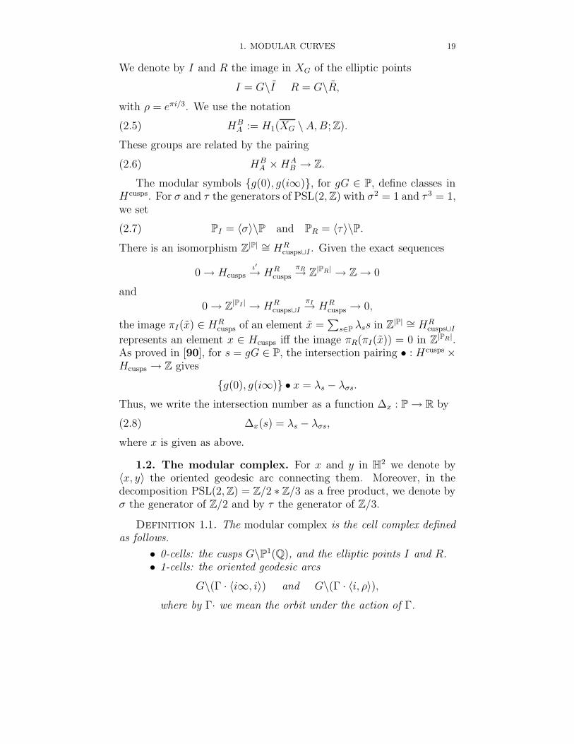
1.2. The modular complex. For x and y in H2 we denote by〈x, y〉 the oriented geodesic arc connecting them. Moreover, in thedecomposition PSL(2, Z) = Z/2 ∗ Z/3 as a free product, we denote byσ the generator of Z/2 and by τ the generator of Z/3.
Definition 1.1. The modular complex is the cell complex definedas follows.
• 0-cells: the cusps G\P1(Q), and the elliptic points I and R.• 1-cells: the oriented geodesic arcs
G\(Γ · 〈i∞, i〉) and G\(Γ · 〈i, ρ〉),where by Γ· we mean the orbit under the action of Γ.
20 2. NONCOMMUTATIVE MODULAR CURVES
Figure 3. The cell decomposition of the modular com-plex
• 2-cells: G\Γ · E, where E is the polygon with vertices
i, ρ, 1 + i, i∞and sides the corresponding geodesic arcs.• Boundary operator: ∂ : C2 → C1 is given by
gE 7→ g〈i, ρ〉+ g〈ρ, 1 + i〉 + g〈1 + i, i∞〉+ g〈i∞, i〉,for g ∈ Γ, and the boundary ∂ : C1 → C0 is given by
g〈i∞, i〉 7→ g(i)− g(i∞)
g〈i, ρ〉 7→ g(ρ)− g(i).
This gives a cell decomposition of H2 adapted to the action ofPSL(2, Z) and congruence subgroups, cf. Figure 3.
We have the following result [81].
Proposition 1.1. The modular complex computes the first homol-ogy of XG:
(2.9) H1(XG) ∼= Ker(∂ : C1 → C0)
Im(∂ : C2 → C1).
We can derive versions of the modular complex that compute rela-tive homology.
Notice that we have Z[cusps] = C0/Z[R ∪ I], hence the quotientcomplex
0→ C2∂→ C1
∂→ Z[cusps]→ 0,
1. MODULAR CURVES 21
with ∂ the induced boundary operator, computes the relative homologyH1(XG, R ∪ I). The cycles are given by Z[P], as combinations of ele-ments g〈i, ρ〉, g ranging over representatives of P, and by the elements⊕ag〈g(i∞), g(i)〉 satisfying
∑agg(i∞) = 0. In fact, these can be rep-
resented as relative cycles in (XG, R ∪ I). Similarly, the subcomplex
0→ Z[P]∂→ Z[R ∪ I]→ 0,
with Z[P] generated by the elements g〈i, ρ〉, computes the homologyH1(XG − cusps). The homology
H1(XG − cusps, R ∪ I) ∼= Z[P]
is generated by the relative cycles g〈i, ρ〉, g ranging over representativesof P.
With the notation (2.5), we consider the groups H cuspsR∪I , HR∪I
cusps,Hcusps, and Hcusps.
We have a long exact sequence of relative homology
(2.10) 0→ Hcusps → HR∪Icusps
(βR,βI)→ H0(R)⊕H0(I)→ Z→ 0,
with Hcusps and HR∪Icusps as above, and with
H0(I) ∼= Z[PI ], PI = 〈σ〉\P = G\I
H0(R) ∼= Z[PR], PR = 〈τ〉\P = G\R,
that is,
(2.11) 0→ Hcusps → Z[P]→ Z[PR]⊕ Z[PI ]→ Z→ 0.
In the case of HR∪Icusps and Hcusps
R∪I the pairing (2.6) gives the identifi-
cation of Z[P] and Z|P|, obtained by identifying the elements of P withthe corresponding delta functions. Thus, we can rewrite the sequence(2.11) as
(2.12) 0→ Hcusps → Z|P| (βR,βI)→ Z|PI | ⊕ Z|PR| → Z→ 0,
where HcuspsR∪I
∼= Z|P|.In order to understand more explicitly the map (βR, βI) we give the
following equivalent algebraic formulation of the modular complex (cf.[81] [90]).
The homology group HR∪Icusps = Z[P] is generated by the images in
XG of the geodesic segments gγ0 := g〈i, ρ〉, with g ranging over a chosenset of representatives of the coset space P.
We can identify (cf. [90]) the dual basis δs of HcuspsR∪I = Z|P| with
the images in XG of the paths gη0, where for a chosen point z0 with
22 2. NONCOMMUTATIVE MODULAR CURVES
0 < <(z0) < 1/2 and |z0| > 1 the path η0 is given by the geodesic arcsconnecting ∞ to z0, z0 to τz0, and τz0 to 0. These satisfy
[gγ0] • [gη0] = 1
[gγ0] • [hη0] = 0,
for gG 6= hG, under the intersection pairing (2.6)Then, in the exact sequence (2.12), the identification of H cusps with
Ker(βR, βI) is obtained by the identification g(0), g(i∞)G 7→ gη0,so that the relations imposed on the generators δs by the vanishingunder βI correspond to the relations δs ⊕ δσs (or δs if s = σs) and thevanishing under βR gives another set of relations δs ⊕ δτs ⊕ δτ2s (or δs
if s = τs).
2. The noncommutative boundary of modular curves
The main idea that bridges between the algebro–geometric theoryof modular curves and noncommutative geometry consists of replacingP1(Q) in the classical compactification, which gives rise to a finite setof cusps, with P1(R). This substitution cannot be done naively, sincethe quotient G\P1(R) is ill behaved topologically, as G does not actdiscretely on P1(R).
When we regard the quotient Γ\P1(R), or more generally a quotientΓ\(P1(R)×P), itself as a noncommutative space, we obtain a geometricobject that is rich enough to recover many important aspects of theclassical theory of modular curves. In particular, it makes sense tostudy in terms of the geometry of such spaces the limiting behavior forcertain arithmetic invariants defined on modular curves when τ → θ ∈R \Q.
2.1. Modular interpretation: noncommutative elliptic curves.
The boundary Γ\P1(R) of the modular curve Γ\H2, viewed itself as anoncommutative space, continues to have a modular interpretation, asobserved originally by Connes–Douglas–Schwarz ([26]). In fact, we canthink of the quotients of S1 by the action of rotations by an irrationalangle (that is, the noncommutative tori) as particular degenerations ofthe classical elliptic curves, which are “invisible” to ordinary algebraicgeometry. The quotient space Γ\P1(R) classifies these noncommutativetori up to Morita equivalence ([16], [101]) and completes the modulispace Γ\H2 of the classical elliptic curves. Thus, from a conceptualpoint of view it is reasonable to think of Γ\P1(R) as the boundary ofΓ\H2, when we allow points in this classical moduli space (that is, el-liptic curves) to have non-classical degenerations to noncommutativetori.
2. THE NONCOMMUTATIVE BOUNDARY OF MODULAR CURVES 23
Noncommutative tori are, in a sense, a prototype example of non-commutative spaces, inasmuch as one can see there displayed the fullrange of techniques of noncommutative geometry (cf. [16], [18]). AsC∗–algebras, noncommutative tori are irrational rotation algebras. Werecall some basic properties of noncommutative tori, which justify theclaim that these algebras behave like a noncommutative version of el-liptic curves. We follow mostly [16] [21] and [101] for this material.
2.2. Irrational rotation and Kronecker foliation.
Definition 2.1. The irrational rotation algebra Aθ, for a givenθ ∈ R, is the universal C∗-algebra C∗(U, V ), generated by two unitaryoperators U and V , subject to the commutation relation
(2.13) UV = e2πiθV U.
The algebra Aθ can be realized as a subalgebra of bounded operatorson the Hilbert spaceH = L2(S1), with the circle S1 ∼= R/Z. For a givenθ ∈ R, we consider two operators, that act on a complete orthonormalbasis en of H as
(2.14) Uen = en+1, V en = e2πinθen.
It is easy to check that these operators satisfy the commutation re-lation (2.13), since, for any f ∈ H we have V Uf (t) = Uf(t − θ) =e2πi(t−θ)f(t− θ), while UV f (t) = e2πitf(t− θ).
The irrational rotation algebra can be described in more geometricterms by the foliation on the usual commutative torus by lines withirrational slope. On T 2 = R2/Z2 one considers the foliation dx = θdy,for x, y ∈ R/Z. The space of leaves is described as X = R/(Z + θZ) 'S1/θZ. This quotient is ill behaved as a classical topological space,hence it cannot be well described by ordinary geometry.
A transversal to the foliation is given for instance by the choiceT = y = 0, T ∼= S1 ∼= R/Z. Then the non-commutative torus isobtained (cf. [16] [21]) as
(2.15) Aθ = (fab) a, b ∈ T in the same leaf where (fab) is a power series b =
∑n∈Z bnV n and each bn is an element
of the algebra C(S1). The multiplication is given by
V hV −1 = h R−1θ ,
with
Rθx = x + θ mod 1.
24 2. NONCOMMUTATIVE MODULAR CURVES
|q| 1
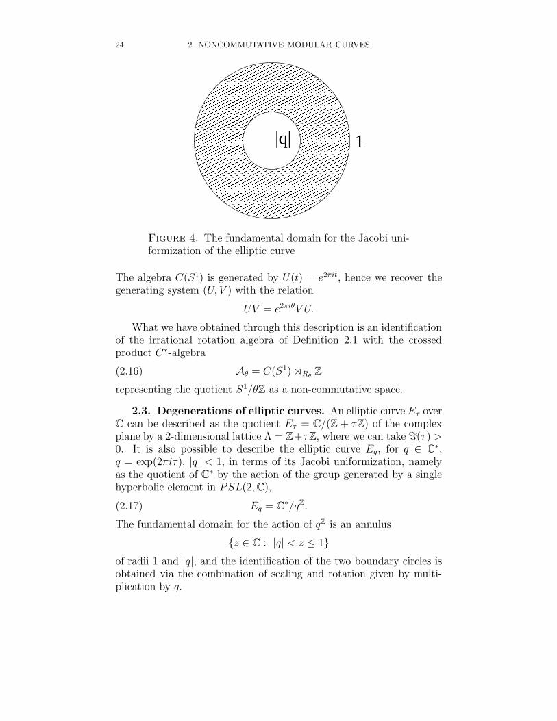
Figure 4. The fundamental domain for the Jacobi uni-formization of the elliptic curve
The algebra C(S1) is generated by U(t) = e2πit, hence we recover thegenerating system (U, V ) with the relation
UV = e2πiθV U.
What we have obtained through this description is an identificationof the irrational rotation algebra of Definition 2.1 with the crossedproduct C∗-algebra
(2.16) Aθ = C(S1) oRθZ
representing the quotient S1/θZ as a non-commutative space.
2.3. Degenerations of elliptic curves. An elliptic curve Eτ overC can be described as the quotient Eτ = C/(Z + τZ) of the complexplane by a 2-dimensional lattice Λ = Z+τZ, where we can take =(τ) >0. It is also possible to describe the elliptic curve Eq, for q ∈ C∗,q = exp(2πiτ), |q| < 1, in terms of its Jacobi uniformization, namelyas the quotient of C∗ by the action of the group generated by a singlehyperbolic element in PSL(2, C),
(2.17) Eq = C∗/qZ.
The fundamental domain for the action of qZ is an annulus
z ∈ C : |q| < z ≤ 1of radii 1 and |q|, and the identification of the two boundary circles isobtained via the combination of scaling and rotation given by multi-plication by q.
2. THE NONCOMMUTATIVE BOUNDARY OF MODULAR CURVES 25
Now let us consider a degeneration where q → exp(2πiθ) ∈ S1,with θ ∈ R \Q. We can say heuristically that in this degeneration theelliptic curve becomes a non-commutative torus
Eq =⇒ Aθ,
in the sense that, as we let q → exp(2πiθ), the annulus of the funda-mental domain shrinks to a circle S1 and we are left with a quotientof S1 by the infinite cyclic group generated by the irrational rotationexp(2πiθ). Since this quotient is ill behaved as a classical quotient,such degenerations do not admit a description within the context ofclassical geometry. However, when we replace the quotient by the cor-responding crossed product algebra C(S1) oθ Z we find the irrationalrotation algebra of definition 2.1. Thus, we can consider such algebrasas non-commutative (degenerate) elliptic curves.
More precisely, when one considers degenerations of elliptic curvesEτ = C∗/qZ for q = e2πiτ , what one obtains in the limit is the suspen-sion of a noncommutative torus. In fact, as the parameter q degeneratesto a point on the unit circle, q → e2πiθ, the “nice” quotient Eτ = C∗/qZ
degenerates to the “bad” quotient Eθ = C∗/e2πiθZ, whose noncommu-tative algebra of coordinates is Morita equivalent to Aθ ⊗ C0(R), withρ ∈ R the radial coordinate, with C∗ 3 z = eρe2πis.
Because of the Thom isomorphism [17], the K-theory of the non-commutative space Eθ = C0(R
2) o (Zθ + Z) satisfies
(2.18) K0(Eθ) = K1(Aθ) and K1(Eθ) = K0(Aθ),
which is again compatible with the identification of the Eθ (rather thanAθ) as degenerations of elliptic curves. In fact, for instance, the Hodgefiltration on the H1 of an elliptic curve and the equivalence betweenthe elliptic curve and its Jacobian have analogs for the noncommutativetorus Aθ in terms of the filtration on HC0 induced by the inclusion ofK0 (cf. [18] p. 132–139, [24] §XIII), while by the Thom isomorphism,these would again appear on the HC1 in the case of the “noncommu-tative elliptic curve” Eθ.
The point of view of degenerations is sometimes a useful guide-line. For instance, one can study the limiting behavior of arithmeticinvariants defined on the parameter space of elliptic curves (on modu-lar curves), in the limit when τ → θ ∈ R \Q. An instance of this typeof result is the theory of limiting modular symbols of [83], which wewill review in this chapter.
2.4. Morita equivalent NC tori. To extend the modular in-terpretation of the quotient Γ\H2 as moduli of elliptic curves to thenoncommutative boundary Γ\P1(R), one needs to check that points
26 2. NONCOMMUTATIVE MODULAR CURVES
in the same orbit of the action of the modular group PSL(2, Z) byfractional linear transformations on P1(R) define equivalent noncom-mutative tori, where equivalence here is to be understood in the Moritasense.
Connes showed in [16] (cf. also [101]) that the noncommutativetori Aθ and A−1/θ are Morita equivalent. Geometrically, in terms ofthe Kronecker foliation and the description (2.15) of the correspondingalgebras, the Morita equivalence Aθ ' A−1/θ corresponds to changingthe choice of the transversal from T = y = 0 to T ′ = x = 0.
In fact, all Morita equivalences arise in this way, by changing thechoice of the transversal of the foliation, so that Aθ and Aθ′ are Moritaequivalent if and only if θ ∼ θ′, under the action of PSL(2, Z).
Connes constructed in [16] explicit bimodules realizing the Moritaequivalences between non-commutative tori Aθ and Aθ′ with
θ′ =aθ + b
cθ + d= gθ,
for
g =
(a bc d
)∈ Γ,
by taking Mθ,θ′ to be the Schwartz space S(R × Z/c), with the rightaction of Aθ
Uf (x, u) = f
(x− cθ + d
c, u− 1
)
V f (x, u) = exp(2πi(x− ud/c))f(x, u)
and the left action of Aθ′
U ′f (x, u) = f
(x− 1
c, u− a
)
V ′f (x, u) = exp
(2πi
(x
cθ + d− u
c
))f(x, u).
2.5. Other properties of NC elliptic curves. There are otherways in which the irrational rotation algebra behaves much like anelliptic curve, most notably the relation between the elliptic curve andits Jacobian (cf. [18] and [24]) and some aspects of the theory of thetafunctions, which we recall briefly.
The commutative torus T 2 = S1× S1 is connected, hence the alge-bra C(T 2) does not contain interesting projections. On the contrary,the noncommutative tori Aθ contain a large family of nontrivial projec-tions. Rieffel in [101] showed that, for a given θ irrational and for allα ∈ (Z⊕Zθ)∩[0, 1], there exists a projection Pα inAθ, with Tr(Pα) = α.
3. LIMITING MODULAR SYMBOLS 27
A different construction of projections in Aθ, given by Boca [8], hasarithmetic relevance, inasmuch as these projections correspond to thetheta functions for noncommutative tori defined by Manin in [77].
A method of constructing projections in C∗-algebras is based onthe following two steps (cf. [101] and [76]):
(1) Suppose given a bimodule AMB. If an element ξ ∈ AMB
admits an invertible ∗-invariant square root 〈ξ, ξ〉1/2B , then the
element µ := ξ〈ξ, ξ〉−1/2B satisfies µ〈µ, µ〉B = µ.
(2) Let µ ∈ AMB be a non-trivial element such that µ〈µ, µ〉B = µ.Then the element P :=A 〈µ, µ〉 is a projection.
In Boca’s construction, one obtains elements ξ from Gaussian ele-ments in some Heisenberg modules, in such a way that the correspond-ing 〈ξ, ξ〉B is a quantum theta function in the sense of Manin [77]. Anintroduction to the relation between the Heisenberg groups and thetheory of theta functions is given in the third volume of Mumford’sTata lectures on theta, [92].
3. Limiting modular symbols
We consider the action of the group Γ = PGL(2, Z) on the up-per and lower half planes H± and the modular curves defined by thequotient XG = G\H±, for G a finite index subgroup of Γ. Then thenoncommutative compactification of the modular curves is obtained byextending the action of Γ on H± to the action on the full
P1(C) = H± ∪ P1(R),
so that we have
(2.19) XG = G\P1(C) = Γ\(P1(C)× P).
Due to the fact that Γ does not act discretely on P1(R), the quotient(2.19) makes sense as a noncommutative space
(2.20) C(P1(C)× P) o Γ.
Here P1(R) ⊂ P1(C) is the limit set of the group Γ, namely theset of accumulation points of orbits of elements of Γ on P1(C). Wewill see another instance of noncommutative geometry arising from theaction of a group of Mobius transformations of P1(C) on its limit set,in the context of the geometry at the archimedean primes of arithmeticvarieties.
28 2. NONCOMMUTATIVE MODULAR CURVES
3.1. Generalized Gauss shift and dynamics. We have de-scribed the boundary of modular curves by the crossed product C∗-algebra
(2.21) C(P1(R)× P) o Γ.
We can also describe the quotient space Γ\(P1(R)×P) in the followingequivalent way. If Γ = PGL(2, Z), then Γ-orbits in P1(R) are the sameas equivalence classes of points of [0, 1] under the equivalence relation
x ∼T y ⇔ ∃n, m : T nx = T my
where Tx = 1/x−[1/x] is the classical Gauss shift of the continued frac-tion expansion. Namely, the equivalence relation is that of having thesame tail of the continued fraction expansion (shift-tail equivalence).
A simple generalization of this classical result yields the following.
Lemma 3.1. Γ orbits in P1(R) × P are the same as equivalenceclasses of points in [0, 1]× P under the equivalence relation
(2.22) (x, s) ∼T (y, t)⇔ ∃n, m : T n(x, s) = T m(y, t)
where T : [0, 1]× P→ [0, 1]× P is the shift
(2.23) T (x, s) =
(1
x−[
1
x
],
(−[1/x] 1
1 0
)· s)
generalizing the classical shift of the continued fraction expansion.
As a noncommutative space, the quotient by the equivalence re-lation (2.22) is described by the C∗-algebra of the groupoid of theequivalence relation
G([0, 1]× P, T ) = ((x, s), m− n, (y, t)) : T m(x, s) = T n(y, t)with objects G0 = ((x, s), 0, (x, s)).
In fact, for any T -invariant subset E ⊂ [0, 1]× P, we can considerthe equivalence relation (2.22). The corresponding groupoid C∗-algebraC∗(G(E, T )) encodes the dynamical properties of the map T on E.
Geometrically, the equivalence relation (2.22) on [0, 1]×P is relatedto the action of the geodesic flow on the horocycle foliation on themodular curves.
3.2. Arithmetic of modular curves and noncommutative
boundary. The result of Lemma 3.1 shows that the properties of thedynamical system T or (2.22) can be used to describe the geometry ofthe noncommutative boundary of modular curves. There are varioustypes of results that can be obtained by this method ([83] [84]), whichwe will discuss in the rest of this chapter.
3. LIMITING MODULAR SYMBOLS 29
(1) Using the properties of this dynamical system it is possibleto recover and enrich the theory of modular symbols on XG,by extending the notion of modular symbols from geodesicsconnecting cusps to images of geodesics in H2 connecting ir-rational points on the boundary P1(R). In fact, the irrationalpoints of P1(R) define limiting modular symbols. In the caseof quadratic irrationalities, these can be expressed in terms ofthe classical modular symbols and recover the generators ofthe homology of the classical compactification by cusps XG.In the remaining cases, the limiting modular symbol vanishesalmost everywhere.
(2) It is possible to reinterpret Dirichlet series related to modu-lar forms of weight 2 in terms of integrals on [0, 1] of certainintersection numbers obtained from homology classes definedin terms of the dynamical system. In fact, even when thelimiting modular symbol vanishes, it is possible to associate anon-trivial cohomology class in XG to irrational points on theboundary, in such a way that an average of the correspondingintersection numbers give Mellin transforms of modular formsof weight 2 on XG.
(3) The Selberg zeta function of the modular curve can be ex-pressed as a Fredholm determinant of the Perron-Frobeniusoperator associated to the dynamical system on the “bound-ary”.
(4) Using the first formulation of the boundary as the noncom-mutative space (2.21) we can obtain a canonical identificationof the modular complex with a sequence of K-groups of theC∗-algebra. The resulting exact sequence for K-groups can beinterpreted, using the description (2.22) of the quotient space,in terms of the Baum–Connes assembly map and the Thomisomorphism.
All this shows that the noncommutative space C(P1(R) × P) o Γ,which we have so far considered as a boundary stratum of C(H2×P)oΓ, in fact contains a good part of the arithmetic information on theclassical modular curve itself. The fact that information on the “bulkspace” is stored in its boundary at infinity can be seen as an instance ofthe physical principle of holography (bulk/boundary correspondence)in string theory (cf. [82]). We will discuss the holography principle inmore details in relation to the geometry of the archimedean fibers ofarithmetic varieties.
30 2. NONCOMMUTATIVE MODULAR CURVES
3.3. Limiting modular symbols. Let γβ be an infinite geodesicin the hyperbolic plane H with one end at i∞ and the other end atβ ∈ R r Q. Let x ∈ γβ be a fixed base point, τ be the geodesic arclength, and y(τ) be the point along γβ at a distance τ from x, towardsthe end β. Let x, y(τ)G denote the homology class in XG determinedby the image of the geodesic arc 〈x, y(τ)〉 in H.
Definition 3.1. The limiting modular symbol is defined as
(2.24) ∗, βG := lim1
τx, y(τ)G ∈ H1(XG, R),
whenever such limit exists.
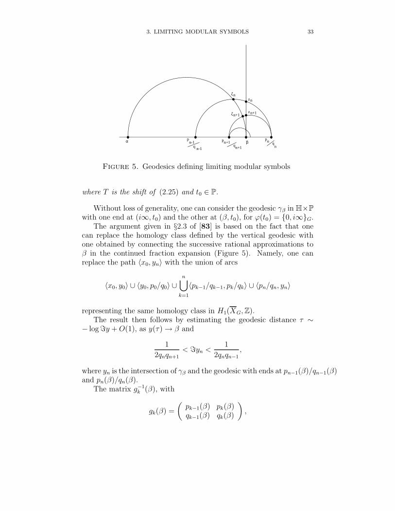
The limit (2.24) is independent of the choice of the initial point xas well as of the choice of the geodesic in H ending at β, as discussedin [83] (cf. Figure 5). We use the notation ∗, βG as introduced in[83], where ∗ in the first argument indicates the independence on thechoice of x, and the double brackets indicate the fact that the homologyclass is computed as a limiting cycle.
3.3.1. Dynamics of continued fractions. As above, we consider on[0, 1]× P the dynamical system
T : [0, 1]× P→ [0, 1]× P
(2.25) T (β, t) =
(1
β−[
1
β
],
(−[1/β] 1
1 0
)· t)
.
This generalizes the classical shift map of the continued fraction
T : [0, 1]→ [0, 1] T (x) =1
x−[
1
x
].
Recall the following basic notation regarding continued fraction ex-pansion. Let k1, . . . , kn be independent variables and, for n ≥ 1, let
[k1, . . . , kn] :=1
k1 + 1k2+... 1
kn
=Pn(k1, . . . , kn)
Qn(k1, . . . , kn).
The Pn, Qn are polynomials with integral coefficients, which can becalculated inductively from the relations
Qn+1(k1, . . . , kn, kn+1) = kn+1Qn(k1, . . . , kn) + Qn−1(k1, . . . , kn−1),
Pn(k1, . . . , kn) = Qn−1(k2, . . . , kn),
with Q−1 = 0, Q0 = 1. Thus, we obtain
[k1, . . . , kn−1, kn + xn]
3. LIMITING MODULAR SYMBOLS 31
=Pn−1(k1, . . . , kn−1) xn + Pn(k1, . . . , kn)
Qn−1(k1, . . . , kn−1) xn + Qn(k1, . . . , kn)=
(Pn−1 Pn
Qn−1 Qn
)(xn),
with the standard matrix notation for fractional linear transformations,
z 7→ az + b
cz + d=
(a bc d
)(z).
If α ∈ (0, 1) is an irrational number, there is a unique sequenceof integers kn(α) ≥ 1 such that α is the limit of [ k1(α), . . . , kn(α) ] asn→∞. Moreover, there is a unique sequence xn(α) ∈ (0, 1) such that
α = [ k1(α), . . . , kn−1(α), kn(α) + xn(α) ]
for each n ≥ 1. We obtain
α =
(0 11 k1(α)
). . .
(0 11 kn(α)
)(xn(α)).
We set
pn(α) := Pn(k1(α), . . . , kn(α)), qn(α) := Qn(k1(α), . . . , kn(α))
so that pn(α)/qn(α) is the sequence of convergents to α. We also set
gn(α) :=
(pn−1(α) pn(α)qn−1(α) qn(α)
)∈ GL(2, Z).
Written in terms of the continued fraction expansion, the shift T isgiven by
T : [k0, k1, k2, . . .] 7→ [k1, k2, k3, . . .].
The properties of the shift (2.25) can be used to extend the no-tion of modular symbols to geodesics with irrational ends ([83]). Suchgeodesics correspond to infinite geodesics on the modular curve XG,which exhibit a variety of interesting possible behaviors, from closedgeodesics to geodesics that approximate some limiting cycle, to geodesicsthat wind around different homology class exhibiting a typically chaoticbehavior.
3.3.2. Lyapunov spectrum. A measure of how chaotic a dynamicalsystem is, or better of how fast nearby orbits tend to diverge, is givenby the Lyapunov exponent.
Definition 3.2. the Lyapunov exponent of T : [0, 1] → [0, 1] isdefined as
(2.26) λ(β) := limn→∞
1
nlog |(T n)′(β)| = lim
n→∞
1
nlog
n−1∏
k=0
|T ′(T kβ)|.
32 2. NONCOMMUTATIVE MODULAR CURVES
The function λ(β) is T–invariant. Moreover, in the case of the clas-sical continued fraction shift Tβ = 1/β − [1/β] on [0, 1], the Lyapunovexponent is given by
(2.27) λ(β) = 2 limn→∞
1
nlog qn(β),
with qn(β) the successive denominators of the continued fraction ex-pansion.
In particular, the Khintchine–Levy theorem shows that, for almostall β’s (with respect to the Lebesgue measure on [0, 1]) the limit (2.27)is equal to
(2.28) λ(β) = π2/(6 log 2) =: λ0.
There is, however, an exceptional set in [0, 1] of Hausdorff dimensiondimH = 1 but with Lebesgue measure zero where the limit defining theLyapunov exponent does not exist.
As we will see later, in “good cases” the value λ(β) can be computedfrom the spectrum of the Perron–Frobenius operator of the shift T .
The Lyapunov spectrum is introduced (cf. [99]) by decomposing theunit interval into level sets of the Lyapunov exponent λ(β) of (2.26).Let Lc = β ∈ [0, 1] |λ(β) = c ∈ R. These sets provide a T–invariantdecomposition of the unit interval,
[0, 1] =⋃
c∈R
Lc ∪ β ∈ [0, 1] |λ(β) does not exist.
These level sets are uncountable dense T–invariant subsets of [0, 1], ofvarying Hausdorff dimension [99]. The Lyapunov spectrum measureshow the Hausdorff dimension varies, as a function h(c) = dimH(Lc).
3.3.3. Limiting modular symbols and iterated shifts. We introducea function ϕ : P→ Hcusps of the form
(2.29) ϕ(s) = g(0), g(i∞)G,
where g ∈ PGL(2, Z) (or PSL(2, Z)) is a representative of the cosets ∈ P.
Then we can compute the limit (2.24) in the following way.
Theorem 3.2. Consider a fixed c ∈ R which corresponds to somelevel set Lc of the Lyapunov exponent (2.27). Then, for all β ∈ Lc, thelimiting modular symbol (2.24) is computed by the limit
(2.30) limn→∞
1
cn
n∑
k=1
ϕ T k(t0),
3. LIMITING MODULAR SYMBOLS 33
zn
zn+1
ζn
pn+1qn+1
pn-1
q n-1
pn qn
ζn+1
α β
Figure 5. Geodesics defining limiting modular symbols
where T is the shift of (2.25) and t0 ∈ P.
Without loss of generality, one can consider the geodesic γβ in H×Pwith one end at (i∞, t0) and the other at (β, t0), for ϕ(t0) = 0, i∞G.
The argument given in §2.3 of [83] is based on the fact that onecan replace the homology class defined by the vertical geodesic withone obtained by connecting the successive rational approximations toβ in the continued fraction expansion (Figure 5). Namely, one canreplace the path 〈x0, yn〉 with the union of arcs
〈x0, y0〉 ∪ 〈y0, p0/q0〉 ∪n⋃
k=1
〈pk−1/qk−1, pk/qk〉 ∪ 〈pn/qn, yn〉
representing the same homology class in H1(XG, Z).The result then follows by estimating the geodesic distance τ ∼
− log=y + O(1), as y(τ)→ β and
1
2qnqn+1< =yn <
1
2qnqn−1,
where yn is the intersection of γβ and the geodesic with ends at pn−1(β)/qn−1(β)and pn(β)/qn(β).
The matrix g−1k (β), with
gk(β) =
(pk−1(β) pk(β)qk−1(β) qk(β)
),
34 2. NONCOMMUTATIVE MODULAR CURVES
acts on points (β, t) ∈ [0, 1]× P as the k–th power of the shift map Tof (2.25). Thus, we obtain
ϕ(T kt0) = g−1k (β) (0), g−1
k (β) (i∞)G =
pk−1(β)
qk−1(β),pk(β)
qk(β)
G
.
3.4. Ruelle and Perron–Frobenius operators. A general prin-ciple in the theory of dynamical systems is that one can often studythe dynamical properties of a map T (e.g. ergodicity) via the spectraltheory of an associated operator. This allows one to employ techniquesof functional analysis and derive conclusions on dynamics.
In our case, to the shift map T of (2.25), we associate the operator
(2.31) (Lσf)(x, t) =
∞∑
k=1
1
(x + k)2σf
(1
x + k,
(0 11 k
)· t)
depending on a complex parameter σ.More generally, the Ruelle transfer operator of a map T is defined
as
(2.32) (Lσf)(x, t) =∑
(y,s)∈T−1(x,t)
exp(h(y, s)) f(y, s),
where we take h(x, t) = −2σ log |T ′(x, t)|. Clearly this operator is wellsuited for capturing the dynamical properties of the map T as it isdefined as a weighted sum over preimages. On the other hand, thereis another operator that can be associated to a dynamical system andwhich typically has better spectral properties, but is less clearly relatedto the dynamics. The best circumstances are when these two agree (fora particular value of the parameter). The other operator is the Perron–Frobenius operator P. This is defined by the relation
(2.33)
∫
[0,1]×P
f (g T ) dµLeb =
∫
[0,1]×P
(P f) g dµLeb.
In the case of the shift T of (2.25) we have in fact that
P = Lσ|σ=1.
3.4.1. Spectral theory of L1. In the case of the modular group G =Γ, the spectral theory of the Perron–Frobenius operator of the Gaussshift was studied by D.Mayer [88]. More recently, Chang and Mayer[14] extended the results to the case of congruence subgroups. A similarapproach is used in [83] to study the properties of the shift (2.25).
3. LIMITING MODULAR SYMBOLS 35
The Perron–Frobenius operator
(L1f)(x, s) =∞∑
k=1
1
(x + k)2f
(1
x + k,
(0 11 k
)· s)
for the shift (2.25) has the following properties.
Theorem 3.3. On a Banach space of holomorphic functions onD×P continuous up to the boundary, with D = z ∈ C | |z−1| < 3/2,under the condition (irreducibility)
(2.34) P = ∪∞n=0
(0 11 k1
). . .
(0 11 kn
)(t0) | k1, . . . , kn ≥ 1
,
the Perron–Frobenius operator L1 has the following properties:
• L1 is a nuclear operator, of trace class.• L1 has top eigenvalue λ = 1. This eigenvalue is simple. The
corresponding eigenfunction is (up to normalization)
1
(1 + x).
• The rest of the spectrum of L1 is contained in a ball of radiusr < 1.• There is a complete set of eigenfunctions.
The irreducibility condition (2.34) is satisfied by congruence sub-groups.
For other T -invariant subsets E ⊂ [0, 1]× P, one can also consideroperators LE,σ and PE. When the set has the property that PE =LE,δE
, for δE = dimH E the Hausdorff dimension, one can use thespectral theory of the operator PE to study the dynamical propertiesof T .
The Lyapunov exponent can be read off the spectrum of the familyof operators LE,σ.
Lemma 3.4. Let λσ denote the top eigenvalue of LE,σ. Then
λ(β) =d
dσλσ|σ=dimH(E) µH a.e. in E
36 2. NONCOMMUTATIVE MODULAR CURVES
3.4.2. The Gauss problem. Let
(2.35) mn(x) := measure of α ∈ (0, 1) | xn(α) ≤ x with α = [ a1(α), . . . , an−1(α), an(α) + xn(α) ].
The asymptotic behavior of the measures mn is a famous problemon the distribution of continued fractions formulated by Gauss, whoconjectured that
(2.36) m(x) = limn→∞
mn(x)?=
1
log 2log(1 + x).
The convergence of (2.35) to (2.36) was only proved by R. Kuzmin in1928. Other proofs were then given by P. Levy (1929), K. Babenko(1978) and D. Mayer (1991). The arguments used by Babenko andMayer use the spectral theory on the Perron–Frobenius operator. Ofthese different arguments only the latter extends nicely to the case ofthe generalized Gauss shift (2.25).
The Gauss problem can be formulated in terms of a recursive rela-tion
(2.37) m′n+1(x) = (L1 m′
n)(x) :=
∞∑
k=1
1
(x + k)2m′
n
(1
x + k
).
The right hand side of (2.37) is the image of m′n under the Gauss–
Kuzmin operator. This is nothing but the Perron–Frobenius operatorfor the shift T in the case of the group Γ = PGL(2, Z).
As a consequence of Theorem 3.3, one obtains the following result.
Theorem 3.5. Let
mn(x, t) := µLeb(y, s) : xn(y) ≤ x, gn(y)−1(s) = t.Then we have
• m′n(x, t) = Ln
1 (1).• The limit m(x, t) = limn→∞ mn(x, t) exists and equals
m(x, t) =1
|P| log 2log(1 + x).
This shows that there exists a unique T -invariant measure on [0, 1]×P. This is uniform in the discrete set P (the counting measure) and itis the Gauss measure of the shift of the continued fraction expansionon [0, 1].
3. LIMITING MODULAR SYMBOLS 37
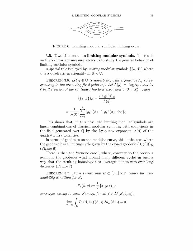
Figure 6. Limiting modular symbols: limiting cycle
3.5. Two theorems on limiting modular symbols. The resulton the T -invariant measure allows us to study the general behavior oflimiting modular symbols.
A special role is played by limiting modular symbols ∗, β whereβ is a quadratic irrationality in R r Q.
Theorem 3.6. Let g ∈ G be hyperbolic, with eigenvalue Λg corre-sponding to the attracting fixed point α+
g . Let Λ(g) := | log Λg|, and let` be the period of the continued fraction expansion of β = α+
g . Then
∗, βG =0, g(0)G
Λ(g)
=1
λ(β)`
∑
k=1
g−1k (β) · 0, g−1
k (β) · i∞G.
This shows that, in this case, the limiting modular symbols arelinear combinations of classical modular symbols, with coefficients inthe field generated over Q by the Lyapunov exponents λ(β) of thequadratic irrationalities.
In terms of geodesics on the modular curve, this is the case wherethe geodesic has a limiting cycle given by the closed geodesic 0, g(0)G
(Figure 6).There is then the “generic case”, where, contrary to the previous
example, the geodesics wind around many different cycles in such away that the resulting homology class averages out to zero over longdistances (Figure 7).
Theorem 3.7. For a T -invariant E ⊂ [0, 1] × P, under the irre-ducibility condition for E,
Rτ (β, s) :=1
τx, y(τ)G
converges weakly to zero. Namely, for all f ∈ L1(E, dµH),
limτ→∞
∫
E
Rτ (β, s) f(β, s) dµH(β, s) = 0.
38 2. NONCOMMUTATIVE MODULAR CURVES
Figure 7. Limiting modular symbols: chaotic tanglingand untangling
This weak convergence can be improved to strong convergence µH(E)-almost everywhere. Thus, the limiting modular symbol satisfies
∗, βG ≡ 0 a.e. on E.
This result depends upon the properties of the operator L1 and theresult on the T -invariant measure. In fact, to get the result on the weakconvergence ([83]) one notices that the limit (2.30) computing limitingmodular symbols can be evaluated in terms of a limit of iterates of thePerron–Frobenius operator, by
limn
1
λ0 n
n∑
k=1
∫
[0,1]×P
f(ϕ T k) = limn
1
λ0n
n∑
k=1
∫
[0,1]×P
(Lk1f)ϕ,
where λ(β) = λ0 a.e. in [0, 1].By the convergence of Lk
11 to the density h of the T -invariant mea-sure and of
Lk1f →
(∫fdµ
)h,
this yields∫
[0,1]×P
∗, β f(β, t) dµ(β, t) =
(∫
[0,1]×P
f dµ
) (∫
[0,1]×P
ϕ h dµ
)
=
(∫f dµ
)1
2#P
∑
s∈P
ϕ(s).
It is then easy to check that the sum∑
s∈Pϕ(s) = 0 since each term in
the sum changes sign under the action of the inversion σ ∈ PGL(2, Z)with σ2 = 1, but the sum is globally invariant under σ.
The argument extends to the case of other T -invariant subsets of[0, 1]×P for which the corresponding Perron–Frobenius operator LE,δE
has analogous properties (cf. [84]). The weak convergence provedby this type of argument can be improved to strong convergence byapplying the strong law of large numbers to the “random variables”ϕk = ϕ T k (cf. [84] for details). The result effectively plays the roleof an ergodic theorem for the shift T on E.
4. HECKE EIGENFORMS 39
4. Hecke eigenforms
A very important question is what happens to modular forms at thenoncommutative boundary of the modular curves. There is a varietyof phenomena in the theory of modular forms that hint to the fact thata suitable class of “modular forms” survives on the noncommutativeboundary. Zagier introduced the term “quantum modular forms” todenote this important and yet not sufficiently understood class of exam-ples. Some aspects of modular forms “pushed” to the noncommutativeboundary were analyzed in [83], in the form of certain averages involv-ing modular symbols and Dirichlet series related to modular forms ofweight 2. We recall here the main results in this case.
We shall now consider the case of congruence subgroups G = Γ0(p),for p a prime.
Let ω be a holomorphic differential (also called a differential of thefirst kind) on the modular curve XΓ0(p) = Γ0(p)\H. Let Φ = ϕ∗(ω)/dzbe the pullback under the projection ϕ : H→ XΓ0(p).
Let Φ be an eigenfunction for all the Hecke operators
Tn =∑
d|n
d−1∑
b=0
(n/d b0 d
)
with (p, n) = 1,
TnΦ = cnΦ.
Then the L-function of ω is given by
Lω(s) = − (2π)s
(2πi)Γ(s)
∫ ∞
0
Φ(iy) ys−1 dy
Lω(s) =∞∑
n=1
cn n−s.
There are many very interesting arithmetic properties of the inte-grals of such Hecke eigenforms on modular symbols (Manin [81]).
In particular, one has ([81]) the following relation between Lω andmodular symbols:
(2.38) (σ(n)− cn) Lω(1) =∑
d|n, b mod d
∫
0,b/d
ω,
with σ(n) =∑
d|n d, from which one obtains
(2.39)
∑q:(q,p)=1 q−(2+t)
∑q′≤q,(q,q′)=1
∫0,q′/q
ω
=[
ζ(p)(1+t)
ζ(p)(2+t)− L
(p)ω (2+t)
ζ(p)(2+t)2
] ∫ i∞
0φ∗(ω)
40 2. NONCOMMUTATIVE MODULAR CURVES
Here L(p)ω is the Mellin transform of Φ with omitted Euler p–factor,
and ζ(s) the Riemann zeta, with corresponding ζ (p), that is, L(p)ω (s) =∑
n:(n,p)=1 cn n−s and ζ (p)(s) =∑
n:(n,p)=1 n−s.
It is therefore interesting to study the properties of integrals onlimiting modular symbols (cf. [83]) and extensions of (2.38) (2.39).
To this purpose, in [83] a suitable class of functions on the boundaryP1(R)× P (or just [0, 1]× P) was introduced.
These are functions of the form
(2.40) `(f, β) =
∞∑
k=1
f(qk(β), qk−1(β)).
Here f is a complex valued function defined on pairs of coprime integers(q, q′) with q ≥ q′ ≥ 1 and with f(q, q′) = O(q−ε) for some ε > 0,and qk(β) are the successive denominators of the continued fractionexpansion of β ∈ [0, 1].
The reason for this choice of functions is given by the followingclassical result of Levy (1929).
Proposition 4.1. For a function f as above, we have
(2.41)
∫ 1
0
`(f, α)dα =∑
q≥q′≥1,(q,q′)=1
f(q, q′)
q(q + q′),
Sums and integrals here converge absolutely and uniformly.
We can interpret the summing over pairs of successive denominatorsas a property that replaces modularity, when “pushed to the bound-ary”.
Through this class of functions it is possible to recast certain aver-ages related to modular symbols on XG, completely in terms of functiontheory on the “boundary” space Γ\(P1(R)×P). A typical result of thissort is the following ([83]).
Upon choosing
f(q, q′) =q + q′
q1+t
∫
0,q′/qG
ω,
one obtains ∫ 1
0
`(f, β) dµLeb(β) =
[ζ(1 + t)
ζ(2 + t)− L
(p)ω (2 + t)
ζ(p)(2 + t)2
] ∫ i∞
0
φ∗(ω),
5. SELBERG ZETA FUNCTION 41
which expresses the Mellin transform of a Hecke eigenform in terms ofa boundary average.
Analogous results exist for different choices of f(q, q ′), for Eisensteinseries twisted by modular symbols, double logarithms at roots of unity,etc.
In fact, this result also shows that, even when the limiting modularsymbol vanishes, one can still associate nontrivial homology classes tothe geodesics with irrational ends.
In fact, for the case of G = Γ0(p) let us consider
(2.42) C(f, β) :=∞∑
n=1
qn+1(β) + qn(β)
qn+1(β)1+t
0,
qn(β)
qn+1(β)
Γ0(p)
.
This defines, for <(t) > 0 and for almost all β, a homology class inH1(XG, cusps, R) such that the integral average
`(f, β) =
∫
C(f,β)
ω
on [0, 1] recovers Mellin transforms of cusp forms by
∫ 1
0
∫
C(f,β)
ω dµLeb(β) =
[ζ(1 + t)
ζ(2 + t)− L
(p)ω (2 + t)
ζ(p)(2 + t)2
] ∫ i∞
0
φ∗(ω).
An estimate
qn+1(β) + qn(β)
qn+1(β)1+t
0,
qn(β)
qn+1(β)
G
∼ e−(5+2t)nλ(β)n∑
k=1
ϕ T k(s)
shows that the series involved are absolutely convergent.
5. Selberg zeta function
Infinite geodesics on XG are the images of infinite geodesics onH2×P with ends on P1(R)×P. Thus, they can be coded by (ω−, ω+, s),with (ω±, s) = endpoints in P1(R) × s, s ∈ P, ω− ∈ (−∞,−1],ω+ ∈ [0, 1].
If ω± are not cusp points, then we have infinite continued fractionexpansions of these endpoints,
ω+ = [k0, k1, . . . kr, kr+1, . . .]ω− = [k−1; k−2, . . . , k−n, k−n−1, . . .]
,
hence the corresponding geodesics are coded by (ω, s), s ∈ P, where ωis a doubly infinite sequence
ω = . . . k−(n+1)k−n . . . k−1k0k1 . . . kn . . .
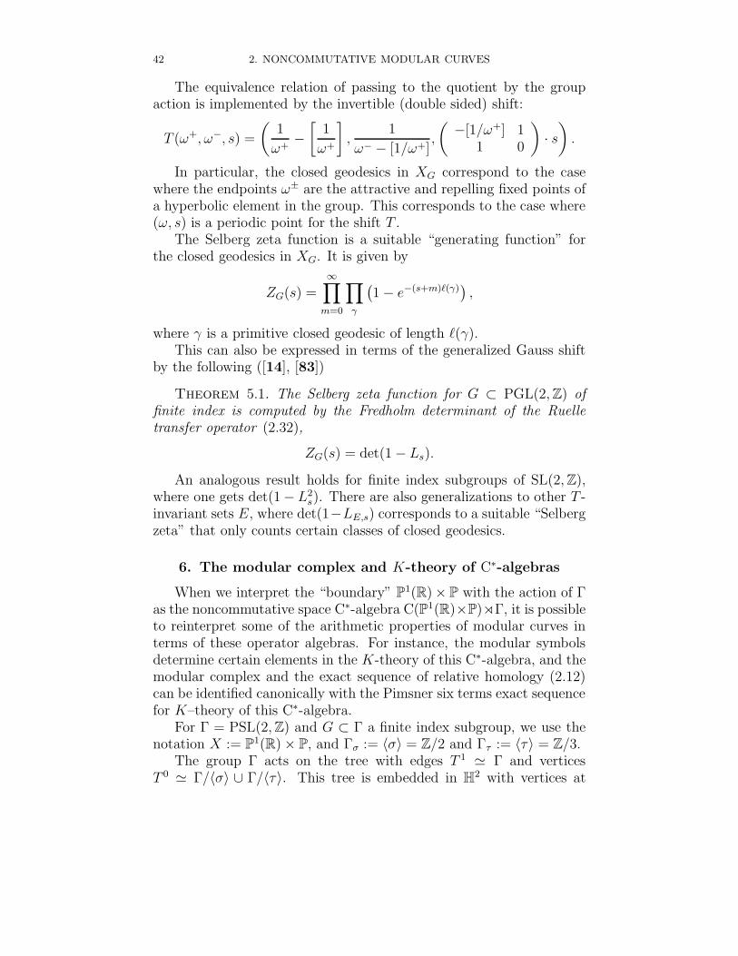
42 2. NONCOMMUTATIVE MODULAR CURVES
The equivalence relation of passing to the quotient by the groupaction is implemented by the invertible (double sided) shift:
T (ω+, ω−, s) =
(1
ω+−[
1
ω+
],
1
ω− − [1/ω+],
(−[1/ω+] 1
1 0
)· s)
.
In particular, the closed geodesics in XG correspond to the casewhere the endpoints ω± are the attractive and repelling fixed points ofa hyperbolic element in the group. This corresponds to the case where(ω, s) is a periodic point for the shift T .
The Selberg zeta function is a suitable “generating function” forthe closed geodesics in XG. It is given by
ZG(s) =∞∏
m=0
∏
γ
(1− e−(s+m)`(γ)
),
where γ is a primitive closed geodesic of length `(γ).This can also be expressed in terms of the generalized Gauss shift
by the following ([14], [83])
Theorem 5.1. The Selberg zeta function for G ⊂ PGL(2, Z) offinite index is computed by the Fredholm determinant of the Ruelletransfer operator (2.32),
ZG(s) = det(1− Ls).
An analogous result holds for finite index subgroups of SL(2, Z),where one gets det(1− L2
s). There are also generalizations to other T -invariant sets E, where det(1−LE,s) corresponds to a suitable “Selbergzeta” that only counts certain classes of closed geodesics.
6. The modular complex and K-theory of C∗-algebras
When we interpret the “boundary” P1(R)× P with the action of Γas the noncommutative space C∗-algebra C(P1(R)×P)oΓ, it is possibleto reinterpret some of the arithmetic properties of modular curves interms of these operator algebras. For instance, the modular symbolsdetermine certain elements in the K-theory of this C∗-algebra, and themodular complex and the exact sequence of relative homology (2.12)can be identified canonically with the Pimsner six terms exact sequencefor K–theory of this C∗-algebra.
For Γ = PSL(2, Z) and G ⊂ Γ a finite index subgroup, we use thenotation X := P1(R)× P, and Γσ := 〈σ〉 = Z/2 and Γτ := 〈τ〉 = Z/3.
The group Γ acts on the tree with edges T 1 ' Γ and verticesT 0 ' Γ/〈σ〉 ∪ Γ/〈τ〉. This tree is embedded in H2 with vertices at
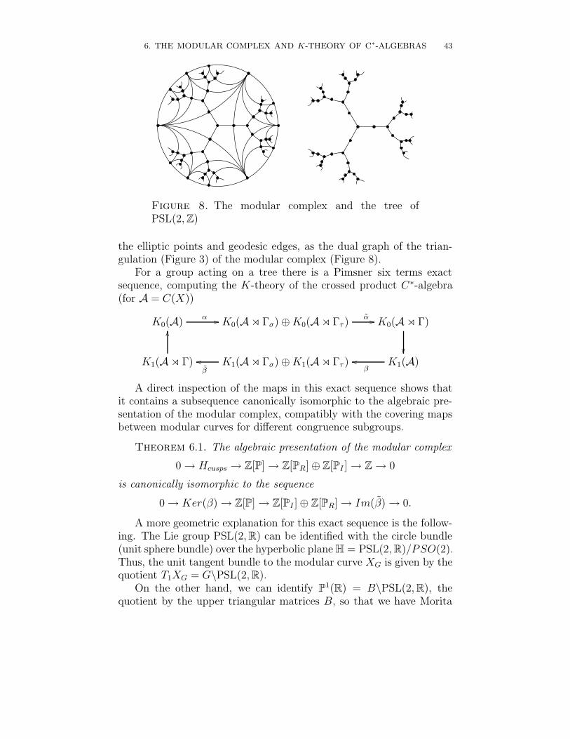
6. THE MODULAR COMPLEX AND K-THEORY OF C∗-ALGEBRAS 43
Figure 8. The modular complex and the tree ofPSL(2, Z)
the elliptic points and geodesic edges, as the dual graph of the trian-gulation (Figure 3) of the modular complex (Figure 8).
For a group acting on a tree there is a Pimsner six terms exactsequence, computing the K-theory of the crossed product C∗-algebra(for A = C(X))
K0(A)α // K0(Ao Γσ)⊕K0(Ao Γτ )
α // K0(Ao Γ)
K1(Ao Γ)
OO
K1(Ao Γσ)⊕K1(Ao Γτ )β
oo K1(A)β
oo
A direct inspection of the maps in this exact sequence shows thatit contains a subsequence canonically isomorphic to the algebraic pre-sentation of the modular complex, compatibly with the covering mapsbetween modular curves for different congruence subgroups.
Theorem 6.1. The algebraic presentation of the modular complex
0→ Hcusps → Z[P]→ Z[PR]⊕ Z[PI ]→ Z→ 0
is canonically isomorphic to the sequence
0→ Ker(β)→ Z[P]→ Z[PI ]⊕ Z[PR]→ Im(β)→ 0.
A more geometric explanation for this exact sequence is the follow-ing. The Lie group PSL(2, R) can be identified with the circle bundle(unit sphere bundle) over the hyperbolic plane H = PSL(2, R)/PSO(2).Thus, the unit tangent bundle to the modular curve XG is given by thequotient T1XG = G\PSL(2, R).
On the other hand, we can identify P1(R) = B\PSL(2, R), thequotient by the upper triangular matrices B, so that we have Morita
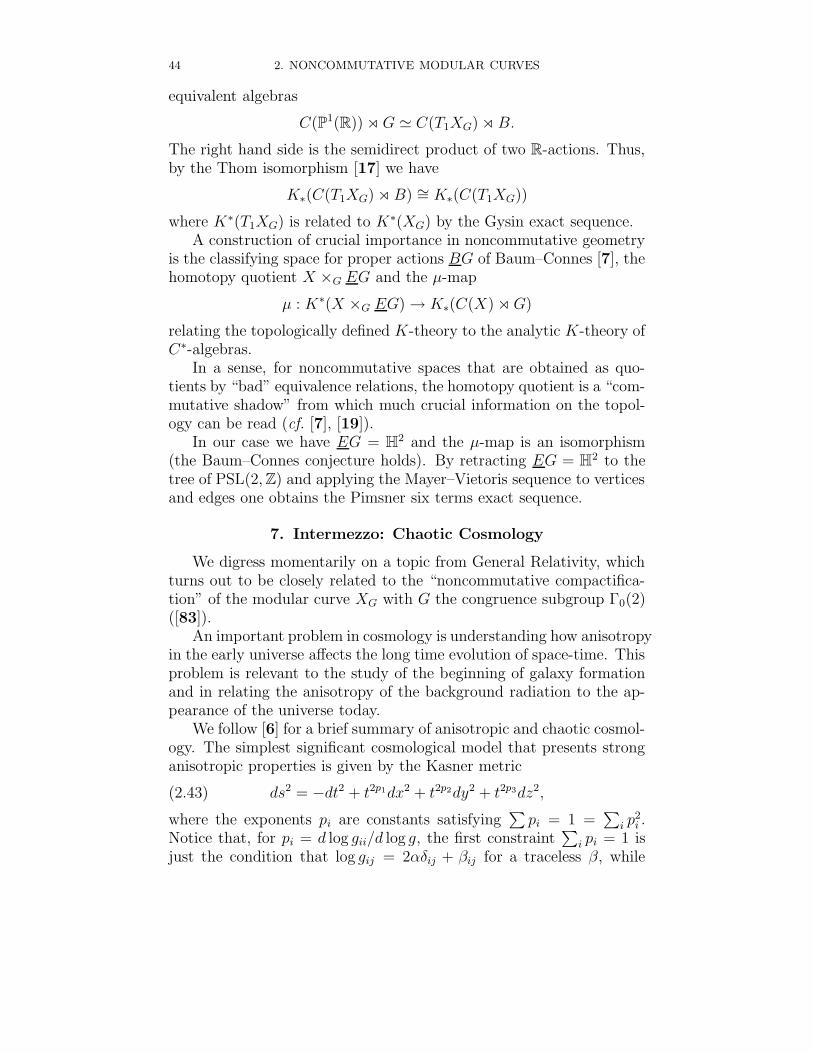
44 2. NONCOMMUTATIVE MODULAR CURVES
equivalent algebras
C(P1(R)) o G ' C(T1XG) o B.
The right hand side is the semidirect product of two R-actions. Thus,by the Thom isomorphism [17] we have
K∗(C(T1XG) o B) ∼= K∗(C(T1XG))
where K∗(T1XG) is related to K∗(XG) by the Gysin exact sequence.A construction of crucial importance in noncommutative geometry
is the classifying space for proper actions BG of Baum–Connes [7], thehomotopy quotient X ×G EG and the µ-map
µ : K∗(X ×G EG)→ K∗(C(X) o G)
relating the topologically defined K-theory to the analytic K-theory ofC∗-algebras.
In a sense, for noncommutative spaces that are obtained as quo-tients by “bad” equivalence relations, the homotopy quotient is a “com-mutative shadow” from which much crucial information on the topol-ogy can be read (cf. [7], [19]).
In our case we have EG = H2 and the µ-map is an isomorphism(the Baum–Connes conjecture holds). By retracting EG = H2 to thetree of PSL(2, Z) and applying the Mayer–Vietoris sequence to verticesand edges one obtains the Pimsner six terms exact sequence.
7. Intermezzo: Chaotic Cosmology
We digress momentarily on a topic from General Relativity, whichturns out to be closely related to the “noncommutative compactifica-tion” of the modular curve XG with G the congruence subgroup Γ0(2)([83]).
An important problem in cosmology is understanding how anisotropyin the early universe affects the long time evolution of space-time. Thisproblem is relevant to the study of the beginning of galaxy formationand in relating the anisotropy of the background radiation to the ap-pearance of the universe today.
We follow [6] for a brief summary of anisotropic and chaotic cosmol-ogy. The simplest significant cosmological model that presents stronganisotropic properties is given by the Kasner metric
(2.43) ds2 = −dt2 + t2p1dx2 + t2p2dy2 + t2p3dz2,
where the exponents pi are constants satisfying∑
pi = 1 =∑
i p2i .
Notice that, for pi = d log gii/d log g, the first constraint∑
i pi = 1 isjust the condition that log gij = 2αδij + βij for a traceless β, while
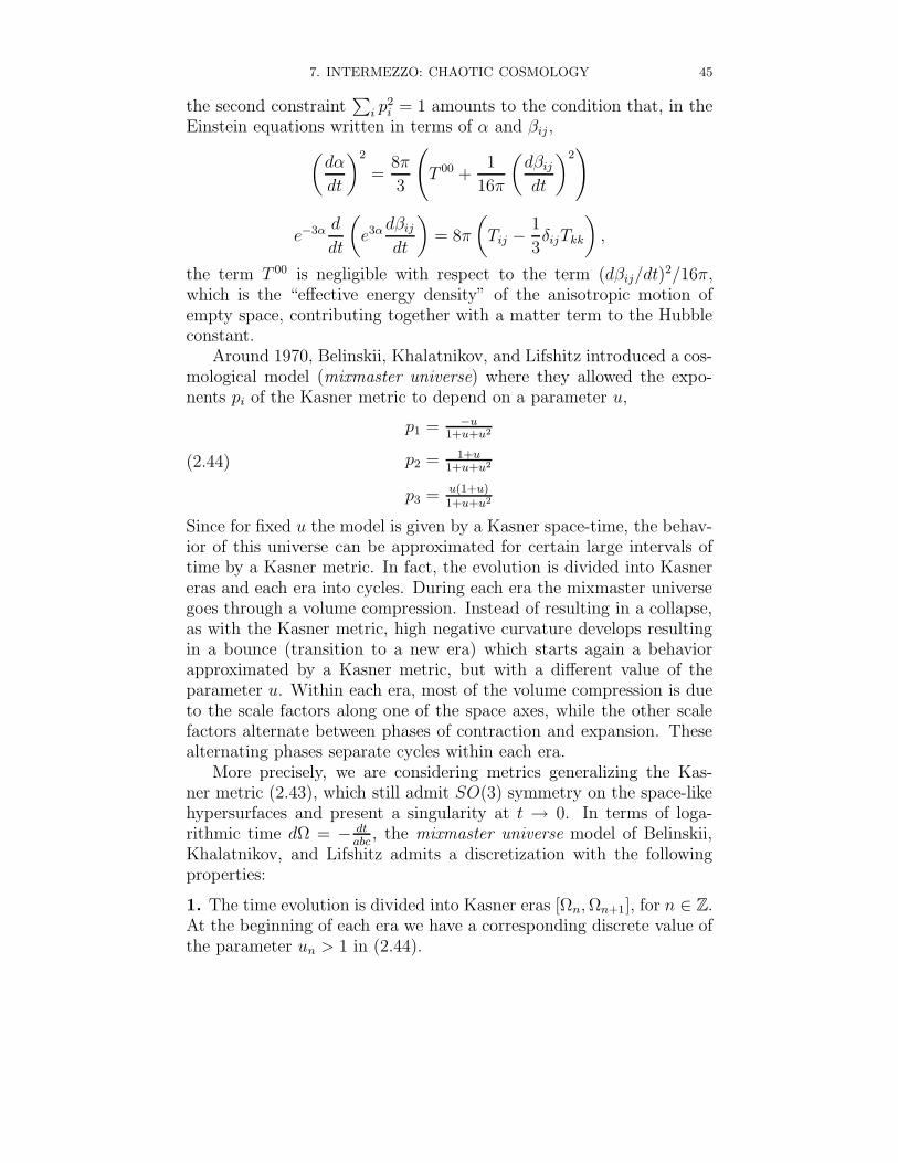
7. INTERMEZZO: CHAOTIC COSMOLOGY 45
the second constraint∑
i p2i = 1 amounts to the condition that, in the
Einstein equations written in terms of α and βij,
(dα
dt
)2
=8π
3
(T 00 +
1
16π
(dβij
dt
)2)
e−3α d
dt
(e3α dβij
dt
)= 8π
(Tij −
1
3δijTkk
),
the term T 00 is negligible with respect to the term (dβij/dt)2/16π,which is the “effective energy density” of the anisotropic motion ofempty space, contributing together with a matter term to the Hubbleconstant.
Around 1970, Belinskii, Khalatnikov, and Lifshitz introduced a cos-mological model (mixmaster universe) where they allowed the expo-nents pi of the Kasner metric to depend on a parameter u,
(2.44)
p1 = −u1+u+u2
p2 = 1+u1+u+u2
p3 = u(1+u)1+u+u2
Since for fixed u the model is given by a Kasner space-time, the behav-ior of this universe can be approximated for certain large intervals oftime by a Kasner metric. In fact, the evolution is divided into Kasnereras and each era into cycles. During each era the mixmaster universegoes through a volume compression. Instead of resulting in a collapse,as with the Kasner metric, high negative curvature develops resultingin a bounce (transition to a new era) which starts again a behaviorapproximated by a Kasner metric, but with a different value of theparameter u. Within each era, most of the volume compression is dueto the scale factors along one of the space axes, while the other scalefactors alternate between phases of contraction and expansion. Thesealternating phases separate cycles within each era.
More precisely, we are considering metrics generalizing the Kas-ner metric (2.43), which still admit SO(3) symmetry on the space-likehypersurfaces and present a singularity at t → 0. In terms of loga-rithmic time dΩ = − dt
abc, the mixmaster universe model of Belinskii,
Khalatnikov, and Lifshitz admits a discretization with the followingproperties:
1. The time evolution is divided into Kasner eras [Ωn, Ωn+1], for n ∈ Z.At the beginning of each era we have a corresponding discrete value ofthe parameter un > 1 in (2.44).
46 2. NONCOMMUTATIVE MODULAR CURVES
2. Each era, where the parameter u decreases with growing Ω, canbe subdivided in cycles corresponding to the discrete steps un, un − 1,un − 2, etc. A change u → u − 1 corresponds, after acting with thepermutation (12)(3) on the space coordinates, to changing u to −u,hence replacing contraction with expansion and conversely. Withineach cycle the space-time metric is approximated by the Kasner metric(2.43) with the exponents pi in (2.44) with a fixed value of u = un−k >1.3. An era ends when, after a number of cycles, the parameter un
falls in the range 0 < un < 1. Then the bouncing is given by thetransition u→ 1/u which starts a new series of cycles with new Kasnerparameters and a permutation (1)(23) of the space axis, in order tohave again p1 < p2 < p3 as in (2.44).
Thus, the transition formula relating the values un and un+1 of twosuccessive Kasner eras is
un+1 =1
un − [un],
which is exactly the shift of the continued fraction expansion, Tx =1/x− [1/x], with xn+1 = Txn and un = 1/xn.
The previous observation is the key to a geometric description ofsolutions of the mixmaster universe in terms of geodesics on a modularcurve (cf. [83]).
Theorem 7.1. Consider the modular curve XΓ0(2). Each infinitegeodesic γ on XΓ0(2) not ending at cusps determines a mixmaster uni-verse.
In fact, an infinite geodesic on XΓ0(2) is the image under the quotientmap
πΓ : H2 × P→ Γ\(H2 × P) ∼= XG,
where Γ = PGL(2, Z), G = Γ0(2), and P = Γ/G ∼= P1(F2) = 0, 1,∞,of an infinite geodesic on H2×P with ends on P1(R)×P. We consider theelements of P1(F2) as labels assigned to the three space axes, accordingto the identification
(2.45)0 = [0 : 1] 7→ z∞ = [1 : 0] 7→ y1 = [1 : 1] 7→ x.
As we have seen, geodesics can be coded in terms of data (ω−, ω+, s)with the action of the shift T .
The data (ω, s) determine a mixmaster universe, with the kn =[un] = [1/xn] in the Kasner eras, and with the transition between
7. INTERMEZZO: CHAOTIC COSMOLOGY 47
subsequent Kasner eras given by xn+1 = Txn ∈ [0, 1] and by the per-mutation of axes induced by the transformation
(−kn 11 0
)
acting on P1(F2). It is easy to verify that, in fact, this acts as thepermutation 0 7→ ∞, 1 7→ 1, ∞ 7→ 0, if kn is even, and 0 7→ ∞,1 7→ 0, ∞ 7→ 1 if kn is odd, that is, after the identification (2.45), asthe permutation (1)(23) of the space axes (x, y, z), if kn is even, or asthe product of the permutations (12)(3) and (1)(23) if kn is odd. Thisis precisely what is obtained in the mixmaster universe model by therepeated series of cycles within a Kasner era followed by the transitionto the next era.
Data (ω, s) and T m(ω, s), m ∈ Z, determine the same solution upto a different choice of the initial time.
There is an additional time-symmetry in this model of the evolu-tion of mixmaster universes (cf. [6]). In fact, there is an additionalparameter δn in the system, which measures the initial amplitude ofeach cycle. It is shown in [6] that this is governed by the evolution ofa parameter
vn =δn+1(1 + un)
1− δn+1
which is subject to the transformation across cycles vn+1 = [un] + v−1n .
By setting yn = v−1n we obtain
yn+1 =1
(yn + [1/xn]),
hence we see that we can interpret the evolution determined by the data(ω+, ω−, s) with the shift T either as giving the complete evolution ofthe u-parameter towards and away from the cosmological singularity,or as giving the simultaneous evolution of the two parameters (u, v)while approaching the cosmological singularity.
This in turn determines the complete evolution of the parameters(u, δ, Ω), where Ωn is the starting time of each cycle. For the explicitrecursion Ωn+1 = Ωn+1(Ωn, xn, yn) see [6].
The result of Theorem 3.5 on the unique T -invariant measure on[0, 1]× P
(2.46) dµ(x, s) =δ(s) dx
3 log(2) (1 + x),
48 2. NONCOMMUTATIVE MODULAR CURVES
implies that the alternation of the space axes is uniform over the timeevolution, namely the three axes provide the scale factor responsiblefor volume compression with equal frequencies.
The Perron-Frobenius operator for the shift (2.25) yields the densityof the invariant measure (2.46) satisfying L1f = f . The top eigenvalueησ of Lσ is related to the topological pressure by ησ = exp(P (σ)).This can be estimated numerically, using the technique of [5] and theintegral kernel operator representation of §1.3 of [83].
The interpretation of solutions in terms of geodesics provides a nat-ural way to single out and study certain special classes of solutions onthe basis of their geometric properties. Physically, such special classesof solutions exhibit different behaviors approaching the cosmologicalsingularity.
For instance, the data (ω+, s) corresponding to an eventually peri-odic sequence k0k1 . . . km . . . of some period a0 . . . a` correspond to thosegeodesics on XΓ0(2) that asymptotically wind around the closed geo-desic identified with the doubly infinite sequence . . . a0 . . . a`a0 . . . a` . . ..Physically, these universes exhibit a pattern of cycles that recurs peri-odically after a finite number of Kasner eras.
Another special class of solutions is given by the Hensley Cantorsets (cf. [85]). These are the mixmaster universes for which there is afixed upper bound N to the number of cycles in each Kasner era.
In terms of the continued fraction description, these solutions cor-respond to data (ω+, s) with ω+ in the Hensley Cantor set EN ⊂ [0, 1].The set EN is given by all points in [0, 1] with all digits in the continuedfraction expansion bounded by N (cf. [62]). In more geometric terms,these correspond to geodesics on the modular curve XΓ0(2) that wanderonly a finite distance into a cusp.
On the set EN the Ruelle and Perron–Frobenius operators are givenby
(2.47) (Lσ,Nf)(x, s) =N∑
k=1
1
(x + k)2σf
(1
x + k,
(0 11 k
)· s)
.
This operator still has a unique invariant measure µN , whose densitysatisfies L2 dimH(EN ),Nf = f , with
dimH(EN) = 1− 6
π2N− 72 log N
π4N2+ O(1/N2)
the Hausdorff dimension of the Cantor set EN . Moreover, the topeigenvalue ησ of Lσ,N is related to the Lyapunov exponent by
λ(x) =d
dσησ|σ=dimH(EN ),
7. INTERMEZZO: CHAOTIC COSMOLOGY 49
for µN -almost all x ∈ EN .A consequence of the characterization of the time evolution in terms
of the dynamical system (2.25) is that we can study global propertiesof suitable moduli spaces of mixmaster universes. For instance, themoduli space for time evolutions of the u-parameter approaching thecosmological singularity as Ω→∞ is given by the quotient of [0, 1]×Pby the action of the shift T .
Similarly, when we restrict to special classes of solutions, e.g. wecan consider the “moduli space” EN × P modulo the action of T . Inthis example, the dynamical system T acting on EN ×P is a subshift offinite type, and the resulting noncommutative space is a Cuntz–Kriegeralgebra [51]. This is an interesting class of C∗-algebras, generated bypartial isometries. Another such algebra will play a fundamental rolein the geometry at arithmetic infinity, which is the topic of the nextlecture.
In the example of the mixmaster dynamics on the Hensley Cantorsets, the shift T is described by the Markov partition
AN = ((k, t), (`, s))|Uk,t ⊂ T (U`,s),
for k, ` ∈ 1, . . . , N, and s, t ∈ P, with sets Uk,t = Uk × t, whereUk ⊂ EN are the clopen subsets where the local inverses of T aredefined,
Uk =
[1
k + 1,1
k
]∩ EN .
This Markov partition determines a matrix AN , with entries (AN )kt,`s =1 if Uk,t ⊂ T (U`,s) and zero otherwise (cf. Figure 9).
Proposition 7.2. The 3× 3 submatrices Ak` = (A(k,t),(`,s))s,t∈P ofthe matrix AN are of the form
Ak` =
0 0 10 1 01 0 0
` = 2m
0 0 11 0 00 1 0
` = 2m + 1
This is just the condition Uk,t ⊂ T (U`,s) written as
(0 11 `
)· s = t,
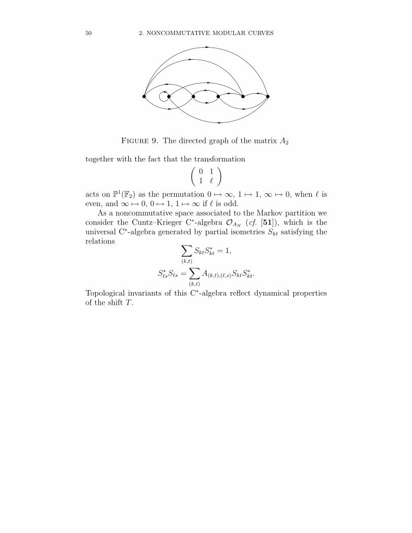
50 2. NONCOMMUTATIVE MODULAR CURVES
Figure 9. The directed graph of the matrix A2
together with the fact that the transformation(0 11 `
)
acts on P1(F2) as the permutation 0 7→ ∞, 1 7→ 1, ∞ 7→ 0, when ` iseven, and ∞ 7→ 0, 0 7→ 1, 1 7→ ∞ if ` is odd.
As a noncommutative space associated to the Markov partition weconsider the Cuntz–Krieger C∗-algebra OAN
(cf. [51]), which is theuniversal C∗-algebra generated by partial isometries Skt satisfying therelations ∑
(k,t)
SktS∗kt = 1,
S∗`sS`s =
∑
(k,t)
A(k,t),(`,s)SktS∗kt.
Topological invariants of this C∗-algebra reflect dynamical propertiesof the shift T .
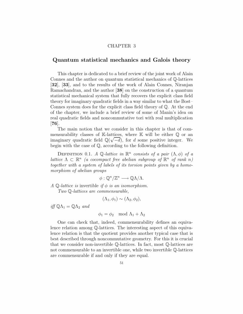
CHAPTER 3
Quantum statistical mechanics and Galois theory
This chapter is dedicated to a brief review of the joint work of AlainConnes and the author on quantum statistical mechanics of Q-lattices[32], [33], and to the results of the work of Alain Connes, NiranjanRamachandran, and the author [38] on the construction of a quantumstatistical mechanical system that fully recovers the explicit class fieldtheory for imaginary quadratic fields in a way similar to what the Bost–Connes system does for the explicit class field theory of Q. At the endof the chapter, we include a brief review of some of Manin’s idea onreal quadratic fields and noncommutative tori with real multiplication[76].
The main notion that we consider in this chapter is that of com-mensurability classes of K-lattices, where K will be either Q or animaginary quadratic field Q(
√−d), for d some positive integer. We
begin with the case of Q, according to the following definition.
Definition 0.1. A Q-lattice in Rn consists of a pair (Λ, φ) of alattice Λ ⊂ Rn (a cocompact free abelian subgroup of Rn of rank n)together with a system of labels of its torsion points given by a homo-morphism of abelian groups
φ : Qn/Zn −→ QΛ/Λ.
A Q-lattice is invertible if φ is an isomorphism.Two Q-lattices are commensurable,
(Λ1, φ1) ∼ (Λ2, φ2),
iff QΛ1 = QΛ2 and
φ1 = φ2 mod Λ1 + Λ2
One can check that, indeed, commensurability defines an equiva-lence relation among Q-lattices. The interesting aspect of this equiva-lence relation is that the quotient provides another typical case that isbest described through noncommutative geometry. For this it is crucialthat we consider non-invertible Q-lattices. In fact, most Q-lattices arenot commensurable to an invertible one, while two invertible Q-latticesare commensurable if and only if they are equal.
51
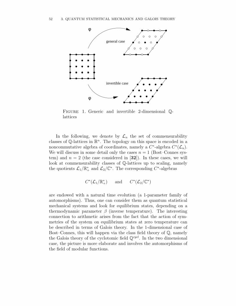
52 3. QUANTUM STATISTICAL MECHANICS AND GALOIS THEORY
φ
φ
general case
invertible case
Figure 1. Generic and invertible 2-dimensional Q-lattices
In the following, we denote by Ln the set of commensurabilityclasses of Q-lattices in Rn. The topology on this space is encoded in anoncommutative algebra of coordinates, namely a C∗-algebra C∗(Ln).We will discuss in some detail only the cases n = 1 (Bost–Connes sys-tem) and n = 2 (the case considered in [32]). In these cases, we willlook at commensurability classes of Q-lattices up to scaling, namelythe quotients L1/R∗
+ and L2/C∗. The corresponding C∗-algebras
C∗(L1/R∗+) and C∗(L2/C∗)
are endowed with a natural time evolution (a 1-parameter family ofautomorphisms). Thus, one can consider them as quantum statisticalmechanical systems and look for equilibrium states, depending on athermodynamic parameter β (inverse temperature). The interestingconnection to arithmetic arises from the fact that the action of sym-metries of the system on equilibrium states at zero temperature canbe described in terms of Galois theory. In the 1-dimensional case ofBost–Connes, this will happen via the class field theory of Q, namelythe Galois theory of the cyclotomic field Qcycl. In the two dimensionalcase, the picture is more elaborate and involves the automorphisms ofthe field of modular functions.
1. QUANTUM STATISTICAL MECHANICS 53
1. Quantum Statistical Mechanics
In classical statistical mechanics a state is a probability measure µon the phase space that assigns to each observable f an expectationvalue, in the form of an average
(3.1)
∫f dµ.
In particular, for a Hamiltonian system, the macroscopic thermody-namic behavior is described via the Gibbs canonical ensemble. This isthe measure
(3.2) dµG =1
Ze−βHdµLiouville,
normalized by Z =∫
e−βHdµLiouville, with a thermodynamic parameterβ = (kT )−1, for T the temperature and k the Boltzmann constant(which we can set equal to one in suitable units).
A quantum statistical mechanical system consists of the data of analgebra of observables (a C∗-algebra A), together with a time evolutiongiven as a 1-parameter family of automorphisms σt ∈ Aut(A). We referto the pair (A, σt) as a C∗-dynamical system. These data describe themicroscopic quantum mechanical evolution of the system.
The macroscopic thermodynamical properties are encoded in theequilibrium states of the system, depending on the inverse tempera-ture β. While the Gibbs measure in the classical case is defined interms of the Hamiltonian and the symplectic structure on the phasespace, the notion of equilibrium state in the quantum statistical me-chanical setting only depends on the algebra of observables and itstime evolution, and does not involve any additional structure like thesymplectic structure or the approximation by regions of finite volume.
We first need to recall the notion of states. These can be thoughtof as probability measures on noncommutative spaces.
Definition 1.1. Given a unital C∗-algebra A, a state on A is alinear functional ϕ : A → C satisfying normalization and positivity,
(3.3) ϕ(1) = 1, ϕ(a∗a) ≥ 0.
When the C∗-algebra A is non-unital, the condition ϕ(1) = 1 is replacedby ‖ϕ‖ = 1 where
(3.4) ‖ϕ‖ := supx∈A,‖x‖≤1|ϕ(x)| .
Such states are restrictions of states on the unital C∗-algebra A ob-tained by adjoining a unit.
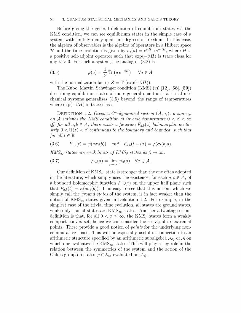
54 3. QUANTUM STATISTICAL MECHANICS AND GALOIS THEORY
Before giving the general definition of equilibrium states via theKMS condition, we can see equilibrium states in the simple case of asystem with finitely many quantum degrees of freedom. In this case,the algebra of observables is the algebra of operators in a Hilbert spaceH and the time evolution is given by σt(a) = eitH a e−itH , where H isa positive self-adjoint operator such that exp(−βH) is trace class forany β > 0. For such a system, the analog of (3.2) is
(3.5) ϕ(a) =1
ZTr(a e−βH
)∀a ∈ A,
with the normalization factor Z = Tr(exp(−βH)).The Kubo–Martin–Schwinger condition (KMS) (cf. [12], [58], [59])
describing equilibrium states of more general quantum statistical me-chanical systems generalizes (3.5) beyond the range of temperatureswhere exp(−βH) is trace class.
Definition 1.2. Given a C∗-dynamical system (A, σt), a state ϕon A satisfies the KMS condition at inverse temperature 0 < β < ∞iff, for all a, b ∈ A, there exists a function Fa,b(z) holomorphic on thestrip 0 < =(z) < β continuous to the boundary and bounded, such thatfor all t ∈ R
(3.6) Fa,b(t) = ϕ(aσt(b)) and Fa,b(t + iβ) = ϕ(σt(b)a).
KMS∞ states are weak limits of KMSβ states as β →∞,
(3.7) ϕ∞(a) = limβ→∞
ϕβ(a) ∀a ∈ A.
Our definition of KMS∞ state is stronger than the one often adoptedin the literature, which simply uses the existence, for each a, b ∈ A, ofa bounded holomorphic function Fa,b(z) on the upper half plane suchthat Fa,b(t) = ϕ(aσt(b)). It is easy to see that this notion, which wesimply call the ground states of the system, is in fact weaker than thenotion of KMS∞ states given in Definition 1.2. For example, in thesimplest case of the trivial time evolution, all states are ground states,while only tracial states are KMS∞ states. Another advantage of ourdefinition is that, for all 0 < β ≤ ∞, the KMSβ states form a weaklycompact convex set, hence we can consider the set Eβ of its extremalpoints. These provide a good notion of points for the underlying non-commutative space. This will be especially useful in connection to anarithmetic structure specified by an arithmetic subalgebra AQ of A onwhich one evaluates the KMS∞ states. This will play a key role in therelation between the symmetries of the system and the action of theGalois group on states ϕ ∈ E∞ evaluated on AQ.
1. QUANTUM STATISTICAL MECHANICS 55
Im z = β
Im z = 0F(t) = ϕ(aσt(b))
F(t + iβ) = ϕ(σt(b)a)
0
iβ
Figure 2. The KMS condition
1.1. Symmetries. An important role in quantum statistical me-chanics is played by symmetries. Typically, symmetries of the algebraA compatible with the time evolution induce symmetries of the equi-librium states Eβ at different temperatures. Especially important arethe phenomena of symmetry breaking. In such cases, there is a globalunderlying group G of symmetries of the algebra A, but in certainranges of temperature the choice of an equilibrium state ϕ breaks thesymmetry to a smaller subgroup Gϕ = g ∈ G : g∗ϕ = ϕ, whereg∗ denotes the induced action on states. Various systems can exhibitone or more phase transitions, or none at all. A typical situation inphysical systems sees a unique KMS state for all values of the parame-ter above a certain critical temperature (β < βc). This corresponds toa chaotic phase such as randomly distributed spins in a ferromagnet.When the system cools down and reaches the critical temperature, theunique equilibrium state branches off into a larger set KMSβ and thesymmetry is broken by the choice of an extremal state in Eβ.
We will see that the case of L1/R∗+ gives rise to a system with a
single phase transition ([9]), while in the case of L2/C∗ the system hasmultiple phase transitions.
A very important point is that we need to consider both symmetriesby automorphisms and by endomorphisms.
Automorphisms: A subgroup G ⊂ Aut(A) is compatible with σt iffor all g ∈ G and for all t ∈ R we have gσt = σtg. There is then an
56 3. QUANTUM STATISTICAL MECHANICS AND GALOIS THEORY
induced action of G on KMS states and in particular on the set Eβ. Ifu is a unitary, acting on A by
Ad u : a 7→ uau∗
and satisfying σt(u) = u, then we say that Ad u is an inner automor-phism of (A, σt). Inner automorphisms act trivially on KMS states.
Endomorphisms: Let ρ be a ∗-homomorphism satisfying ρσt = σtρ.Consider the idempotent e = ρ(1). If ϕ ∈ Eβ is a state such thatϕ(e) 6= 0, then there is a well defined pullback ρ∗ϕ,
(3.8) ρ∗(ϕ) =1
ϕ(e)ϕ ρ.
Let u be an isometry compatible with the time evolution by
(3.9) σt(u) = λitu λ > 0.
One has u∗u = 1 and uu∗ = e. We say that Ad u defined by a 7→ uau∗
is an inner endomorphism of (A, σt). The condition (3.9) ensures that(Adu)∗ϕ is well defined according to (3.8) and the KMS conditionshows that the induced action of an inner endomorphism on KMS statesis trivial.
One needs to be especially careful in defining the action of endo-morphisms by (3.8). In fact, there are cases where for KMS∞ statesone finds only ϕ(e) = 0, yet it is still possible to define an interestingaction of endomorphisms by a procedure of “warming up and coolingdown”. For this to work one needs sufficiently favorable conditions,namely that the “warming up” map
(3.10) Wβ(ϕ)(a) =Tr(πϕ(a) e−β H)
Tr( e−β H)
gives a homeomorphism Wβ : E∞ → Eβ for all β sufficiently large. Onecan then define the action by
(3.11) (ρ∗ϕ)(a) = limβ→∞
(ρ∗Wβ(ϕ)) (a),
for all ϕ ∈ E∞ and all a ∈ A.
2. The Bost–Connes system
We give the following geometric point of view on the BC system,following [38].
We use the notation Sh(G, X) := G(Q)\(G(Af )×X) for Shimura
varieties (cf. [91]). Here Af = Z ⊗ Q denotes the finite adeles of Q,
2. THE BOST–CONNES SYSTEM 57
with Z = lim←−nZ/nZ. The simplest case is for G = GL1, where we
consider
(3.12) Sh(GL1, ±1) = GL1(Q)\(GL1(Af)× ±1) = Q∗+\A∗
f .
Lemma 2.1. The quotient (3.12) parameterizes the invertible 1-dimensional Q-lattices up to scaling.
In fact, first notice that a 1-dimensional Q-lattice can always bewritten in the form
(3.13) (Λ, φ) = (λ Z, λ ρ)
for some λ > 0 and some
(3.14) ρ ∈ Hom(Q/Z, Q/Z) = lim←−Z/nZ = Z.
Thus, the set of 1-dimensional Q-lattices up to scaling can be identifiedwith Z. The invertible lattices correspond to the elements of Z∗, whichin turn is identified with GL+
1 (Q)\GL1(Af).The quotient (3.12) can be thought of geometrically as the Shimura
variety associated to the cyclotomic tower (cf. [38]). This is the tower Vof arithmetic varieties over V = Spec(Z), with Vn = Spec(Z[ζn]), whereζn is a primitive n-th root of unity. The group of deck transformationsis AutV (Vn) = GL1(Z/nZ), so that the group of deck transformationsof the tower is the projective limit
(3.15) AutV (V) = lim←−n
AutV (Vn) = GL1(Z).
If, instead of invertible Q-lattices up to scale, we consider the setof commensurability classes of all 1-dimensional Q-lattices up to scale,we find a noncommutative version of the Shimura variety (3.12) and ofthe cyclotomic tower. This is described as the quotient
(3.16) Sh(nc)(GL1, ±1) := GL1(Q)\(Af×±1) = GL1(Q)\A·/R∗+,
where A· := Af × R∗ are the adeles of Q with invertible archimedeancomponent.
The corresponding noncommutative algebra of coordinates is givenby the crossed product (cf. [68])
(3.17) C0(Af ) o Q∗+.
One obtains an equivalent description of the noncommutative space(3.16), starting from the description (3.13) of 1-dimensional Q-lattices.The commensurability relation is implemented by the action of N× =Z>0 by
(3.18) αn(f)(ρ) =
f(n−1ρ) ρ ∈ nZ0 otherwise.
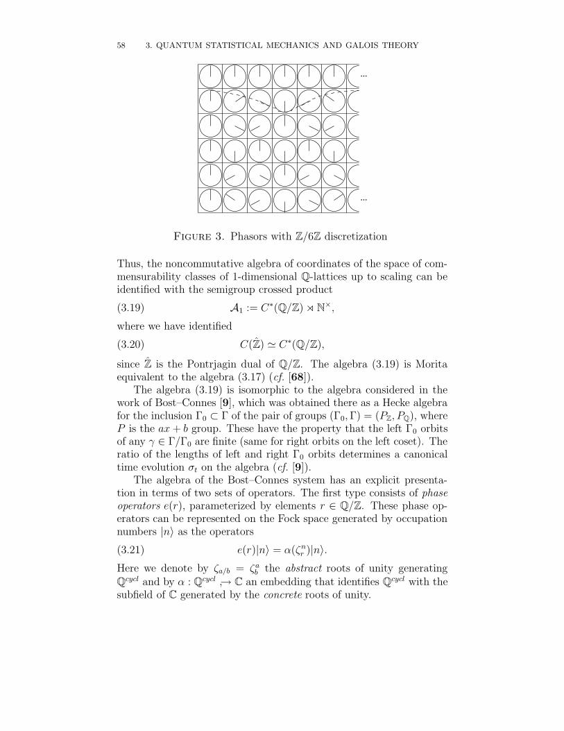
58 3. QUANTUM STATISTICAL MECHANICS AND GALOIS THEORY
...
...
Figure 3. Phasors with Z/6Z discretization
Thus, the noncommutative algebra of coordinates of the space of com-mensurability classes of 1-dimensional Q-lattices up to scaling can beidentified with the semigroup crossed product
(3.19) A1 := C∗(Q/Z) o N×,
where we have identified
(3.20) C(Z) ' C∗(Q/Z),
since Z is the Pontrjagin dual of Q/Z. The algebra (3.19) is Moritaequivalent to the algebra (3.17) (cf. [68]).
The algebra (3.19) is isomorphic to the algebra considered in thework of Bost–Connes [9], which was obtained there as a Hecke algebrafor the inclusion Γ0 ⊂ Γ of the pair of groups (Γ0, Γ) = (PZ, PQ), whereP is the ax + b group. These have the property that the left Γ0 orbitsof any γ ∈ Γ/Γ0 are finite (same for right orbits on the left coset). Theratio of the lengths of left and right Γ0 orbits determines a canonicaltime evolution σt on the algebra (cf. [9]).
The algebra of the Bost–Connes system has an explicit presenta-tion in terms of two sets of operators. The first type consists of phaseoperators e(r), parameterized by elements r ∈ Q/Z. These phase op-erators can be represented on the Fock space generated by occupationnumbers |n〉 as the operators
(3.21) e(r)|n〉 = α(ζnr )|n〉.
Here we denote by ζa/b = ζab the abstract roots of unity generating
Qcycl and by α : Qcycl → C an embedding that identifies Qcycl with thesubfield of C generated by the concrete roots of unity.
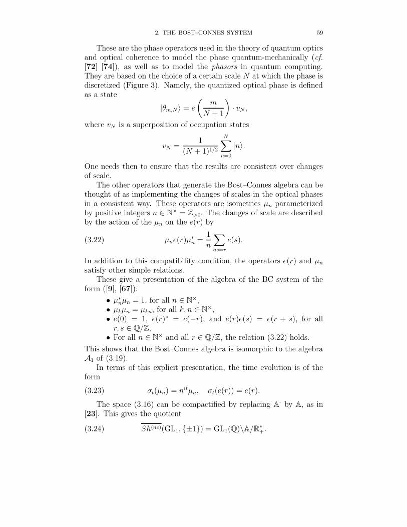
2. THE BOST–CONNES SYSTEM 59
These are the phase operators used in the theory of quantum opticsand optical coherence to model the phase quantum-mechanically (cf.[72] [74]), as well as to model the phasors in quantum computing.They are based on the choice of a certain scale N at which the phase isdiscretized (Figure 3). Namely, the quantized optical phase is definedas a state
|θm,N 〉 = e
(m
N + 1
)· vN ,
where vN is a superposition of occupation states
vN =1
(N + 1)1/2
N∑
n=0
|n〉.
One needs then to ensure that the results are consistent over changesof scale.
The other operators that generate the Bost–Connes algebra can bethought of as implementing the changes of scales in the optical phasesin a consistent way. These operators are isometries µn parameterizedby positive integers n ∈ N× = Z>0. The changes of scale are describedby the action of the µn on the e(r) by
(3.22) µne(r)µ∗n =
1
n
∑
ns=r
e(s).
In addition to this compatibility condition, the operators e(r) and µn
satisfy other simple relations.These give a presentation of the algebra of the BC system of the
form ([9], [67]):
• µ∗nµn = 1, for all n ∈ N×,
• µkµn = µkn, for all k, n ∈ N×,• e(0) = 1, e(r)∗ = e(−r), and e(r)e(s) = e(r + s), for all
r, s ∈ Q/Z,• For all n ∈ N× and all r ∈ Q/Z, the relation (3.22) holds.
This shows that the Bost–Connes algebra is isomorphic to the algebraA1 of (3.19).
In terms of this explicit presentation, the time evolution is of theform
(3.23) σt(µn) = nitµn, σt(e(r)) = e(r).
The space (3.16) can be compactified by replacing A· by A, as in[23]. This gives the quotient
(3.24) Sh(nc)(GL1, ±1) = GL1(Q)\A/R∗+.
60 3. QUANTUM STATISTICAL MECHANICS AND GALOIS THEORY
This compactification consists of adding the trivial lattice (with a pos-sibly nontrivial Q-structure).
The dual space to (3.24), under the duality of type II and typeIII factors introduced in Connes’ thesis, is a principal R∗
+-bundle over(3.24), whose noncommutative algebra of coordinates is obtained fromthe algebra of (3.24) by taking the crossed product by the time evolu-tion σt. The space obtained this way is the space of adele classes
(3.25) L1 = GL1(Q)\A→ GL1(Q)\A/R∗+
that gives the spectral realization of zeros of the Riemann ζ functionin [23]. Passing to this dual space corresponds to considering commen-surability classes of 1-dimensional Q-lattices (no longer up to scaling).
2.1. Structure of KMS states. The Bost–Connes algebra A1
has irreducible representations on the Hilbert spaceH = `2(N×). These
are parameterized by elements α ∈ Z∗ = GL1(Z). Any such elementdefines an embedding α : Qcycl → C and the corresponding represen-tation is of the form
(3.26)πα(e(r)) εk = α(ζk
r ) εk
πα(µn) εk = εnk
The Hamiltonian implementing the time evolution (3.18) on H is
(3.27) H εk = (log k) εk
Thus, the partition function of the Bost–Connes system is the Riemannzeta function
(3.28) Z(β) = Tr(e−βH
)=
∞∑
k=1
k−β = ζ(β).
Bost and Connes showed in [9] that KMS states have the followingstructure, with a phase transition at β = 1.
• In the range β ≤ 1 there is a unique KMSβ state. Its restrictionto Q[Q/Z] is of the form
ϕβ(e(a/b)) = b−β∏
p prime, p|b
1− pβ−1
1− p−1.
• For 1 < β ≤ ∞ the set of extremal KMS states Eβ can be
identified with Z∗. It has a free and transitive action of thisgroup induced by an action on A by automorphisms. Theextremal KMSβ state corresponding to α ∈ Z∗ is of the form
(3.29) ϕβ,α(x) =1
ζ(β)Tr(πα(x) e−βH
).
3. NONCOMMUTATIVE GEOMETRY AND HILBERT’S 12TH PROBLEM 61
• At β =∞ the Galois group Gal(Qcycl/Q) acts on the values ofstates ϕ ∈ E∞ on an arithmetic subalgebra A1,Q ⊂ A1. Thesehave the property that ϕ(AQ) ⊂ Qcycl and that the isomor-
phism (class field theory isomorphism) θ : Gal(Qcycl/Q)∼=→ Z∗
intertwines the Galois action on values with the action of Z∗
by symmetries, namely,
(3.30) γ ϕ(x) = ϕ(θ(γ) x),
for all ϕ ∈ E∞, for all γ ∈ Gal(Qcycl/Q) and for all x ∈ AQ.
Here the arithmetic subalgebra A1,Q can be taken to be the algebraover Q generated by the e(r) and the µn, µ
∗n. This Q-algebra can also be
obtained (as shown in [32]) as the algebra generated by the µn, µ∗n and
by homogeneous functions of weight zero on 1-dim Q-lattices obtainedas a normalization of the functions
(3.31) εk,a(Λ, φ) =∑
y∈Λ+φ(a)
y−k
by covolume. Namely, one considers the functions ek,a := ck εk,a, wherec(Λ) is proportional to the covolume |Λ| and satisfies
(2π√−1) c(Z) = 1.
The choice of an “arithmetic subalgebra” corresponds to endowingthe noncommutative space A with an arithmetic structure. The sub-algebra corresponds to the rational functions and the values of KMS∞
states at elements of this subalgebra should be thought of as valuesof “rational functions” at the classical points of the noncommutativespace (cf. [38]).
3. Noncommutative Geometry and Hilbert’s 12th problem
The most remarkable arithmetic feature of the result of Bost–Connesrecalled above is the Galois action on the ground states of the sys-tem. First of all, the fact that the Galois action on the values ofstates would preserve positivity (i.e. would give values of other states)is a very unusual property. Moreover, the values of extremal groundstates on elements of the rational subalgebra generate the maximalabelian extension Qab = Qcycl of Q. The explicit action of the Galoisgroup Gal(Qab/Q) ' GL1(Z) is given by automorphisms of the system(A1, σt). Namely, the class field theory isomorphism intertwines theaction of the idele class group, as symmetry group of the system, andthat of the Galois group, as permutations of the expectation values ofthe rational observables.
62 3. QUANTUM STATISTICAL MECHANICS AND GALOIS THEORY
In general, the main theorem of class field theory provides a classi-fication of finite abelian extensions of a local or global field K in termsof subgroups of a locally compact abelian group canonically associatedto the field. This is the multiplicative group K∗ = GL1(K) in the localnonarchimedean case, while in the global case it is the quotient CK/DK
of the idele class group CK by the connected component of the identity.Hilbert’s 12th problem can be formulated as the question of provid-
ing an explicit set of generators of the maximal abelian extension Kab
of a number field K, inside an algebraic closure K, and of the action ofthe Galois group Gal(Kab/K). The maximal abelian extension Kab ofK has the property that
Gal(Kab/K) = Gal(K/K)ab.
The result that motivated Hilbert’s formulation of the explicit classfield theory problem is the Kronecker–Weber theorem, namely the al-ready mentioned case of the explicit class field theory of K = Q. Inthis case, the maximal abelian extension of Q can be identified withthe cyclotomic field Qcycl. Equivalently, one can say that the torsionpoints of the multiplicative group C∗ (i.e. the roots of unity) generateQab ⊂ C.
Remarkably, the only other case for number fields where this pro-gram has been carried out completely is that of imaginary quadraticfields, where the construction relies on the theory of elliptic curveswith complex multiplication, and on the Galois theory of the field ofmodular functions (cf. e.g. the survey [106]).
Some generalizations of the original result of Bost–Connes to otherglobal fields (number fields and function fields) were obtained by Harariand Leichtnam [60], P. Cohen [15], Arledge, Laca and Raeburn [4]. Amore detailed account of various results related to the BC system andgeneralizations is given in the “further developments” section of [32].Because of this close relation to Hilbert’s 12th problem, it is clear thatfinding generalizations of the Bost–Connes system to other numberfields is a very difficult problem, hence it is not surprising that, so far,these constructions have not fully recovered the Galois properties ofthe ground states of the BC system in the generalized setting.
The strongest form of the result one may wish to obtain in thisdirection can be formulated as follows.
Given a number field K, we let AK denote the adeles of K and welet A∗
K = GL1(AK) be the group of ideles of K. As above, we write CK
for the group of idele classes CK = A∗K/K∗ and DK for the connected
component of the identity in CK.
3. NONCOMMUTATIVE GEOMETRY AND HILBERT’S 12TH PROBLEM 63
One wishes to construct a C∗-dynamical system (AK, σt) and an“arithmetic” subalgebra AK,Q, which satisfy the following properties:
(1) The idele class group G = CK/DK acts by symmetries on(AK, σt) preserving the subalgebra AK,Q.
(2) The states ϕ ∈ E∞, evaluated on elements of AK,Q, satisfy:• ϕ(a) ∈ K, the algebraic closure of K in C;• the elements of ϕ(a) : a ∈ AK,Q, for ϕ ∈ E∞ generate
Kab.(3) The class field theory isomorphism
θ : Gal(Kab/K)'−→ CK/DK
intertwines the actions,
(3.32) α ϕ = ϕ θ(α),
for all α ∈ Gal(Kab/K) and for all ϕ ∈ E∞.
The arithmetic subalgebra AK,Q, in general, need not be an involutivesubalgebra.
The setup described above may provide a possible new approach,via noncommutative geometry, to the explicit class field theory prob-lem.
Given a number field K with [K : Q] = n, there is an embeddingK∗ → GLn(Q) of its multiplicative group in GLn(Q). Such embeddinginduces an embedding of GL1(AK,f) into GLn(Af), where AK,f = Af⊗K
are the finite adeles of K.This suggests that a possible strategy to approach the problem
stated above may be to first study quantum statistical mechanical sys-tems corresponding to GLn analogs of the Bost–Connes system.
The main result of the joint work of Alain Connes and the authorin [32] is the construction of such a system in the GL2 case and theanalysis of the arithmetic properties of its KMS states. In the case ofGL2, one sees that the geometry of modular curves and the algebra ofmodular forms appear naturally.
In joint work of Alain Connes, Niranjan Ramachandran, and theauthor [38], a quantum statistical mechanical system is constructed,which satisfies all the properties listed above for the case where K is animaginary quadratic field. The properties of this system are intermedi-ate between those of the original Bost–Connes system and those of theGL2 system of [32]. In fact, geometrically the construction is based onreplacing the 1-dimensional Q-lattices of the Bost–Connes system with1-dimensional K-lattices. The groupoid of the commensurability rela-tion is then a subgroupoid of that of the GL2-system (1-dimensional
64 3. QUANTUM STATISTICAL MECHANICS AND GALOIS THEORY
K-lattices are a special class of 2-dimensional Q-lattices with compat-ible notions of commensurability). Thus, by combining the techniquesof the Bost–Connes and of the GL2 system, it is possible to show thatthe complex multiplication (CM) system defined this way recovers thefull picture of the explicit class field theory of imaginary quadratic fields[38], as we will recall in this chapter.
The first case for which there is not yet a complete solution to theexplicit class field theory problem is the case of real quadratic fields,K = Q(
√d), for some positive integer d. It is natural to ask whether
the approach outlined above, based on noncommutative geometry, mayprovide any new information on this case. Recent work of Manin [75][76] suggests a close relation between the real quadratic case and non-commutative geometry. We will discuss the possible relation betweenhis approach and the GL2-system.
4. The GL2 system
In this section we will describe the main features of the GL2 analogof the Bost–Connes system, according to the results of [32].
We can start with the same geometric approach in terms of Shimuravarieties (cf. [38], [33]) that we used above to introduce the BC system.
The Shimura variety associated to the tower of modular curves isdescribed by the adelic quotient(3.33)
Sh(GL2, H±) = GL2(Q)\(GL2(Af)×H±)
= GL+2 (Q)\(GL2(Af )×H) = GL+
2 (Q)\GL2(A)/C∗.
The tower of modular curves (cf. [38]) has base V = P1 over Q andVn = X(n) the modular curve corresponding to the principal congru-ence subgroup Γ(n). The automorphisms of the projection Vn → V aregiven by GL2(Z/nZ)/±1, so that the group of deck transformationsof the tower V is in this case of the form
(3.34) AutV (V) = lim←−n
GL2(Z/nZ)/±1 = GL2(Z)/±1.
The inverse limit lim←−Γ\H over congruence subgroups Γ ⊂ SL(2, Z)gives a connected component of (3.33), while by taking congruencesubgroups in SL(2, Q) one obtains the adelic version Sh(GL2, H
±). Thesimple reason why it is necessary to pass to the nonconnected case isthe following. The varieties in the tower are arithmetic varieties definedover number fields. However, the number field typically changes alongthe levels of the tower (Vn is defined over the cyclotomic field Q(ζn)).Passing to nonconnected Shimura varieties allows for the definition of a
4. THE GL2 SYSTEM 65
canonical model where the whole tower is defined over the same numberfield.
The quotient (3.33) parameterizes invertible 2-dimensional Q-latticesup to scaling (cf. [91]). When, instead of restricting to the invertiblecase, we consider commensurability classes of 2-dimensional Q-latticesup to scaling, we obtain a noncommutative space whose classical pointsare the Shimura variety (3.33). More precisely, we have the following(cf. [38]):
Lemma 4.1. The space of commensurability classes of 2-dimensionalQ-lattices up to scaling is described by the quotient
(3.35) Sh(nc)(GL2, H±) := GL2(Q)\(M2(Af)×H±).
Any 2-dimensional Q-lattice can be written in the form
(Λ, φ) = (λ(Z + Zτ), λρ),
for some λ ∈ C∗, some τ ∈ H, and some
ρ ∈M2(Z) = Hom(Q2/Z2, Q2/Z2).
Thus, the space of 2-dimensional Q-lattices up to the scale factor λ ∈C∗ and up to isomorphisms, is given by
(3.36) M2(Z)×H mod Γ = SL(2, Z).
The commensurability relation is implemented by the partially definedaction of GL+
2 (Q) on this space, given by
g(ρ, z) = (gρ, g(z)),
where g(z) denotes action as fractional linear transformation.Commensurability classes of Q-lattices (Λ, φ) in C are equivalent
to isogeny classes of pairs (E, η) of an elliptic curve E = C/Λ and anAf -homomorphism
(3.37) η : Q2 ⊗ Af → Λ⊗ Af ,
where Λ⊗ Af = (Λ⊗ Z)⊗Q, with
(3.38) Λ⊗ Z = lim←−n
Λ/nΛ,
and Λ/nΛ = E[n] the n-torsion of E. Since the Q-lattices need not beinvertible, we do not require that η be an Af -isomorphism (cf. [91]).The commensurability relation between Q-lattices corresponds to theequivalence (E, η) ∼ (E ′, η′) given by an isogeny g : E → E ′ and η′ =(g ⊗ 1) η. Namely, the equivalence classes can be identified with thequotient of M2(Af)×H± by the action of GL2(Q), (ρ, z) 7→ (gρ, g(z)).
66 3. QUANTUM STATISTICAL MECHANICS AND GALOIS THEORY
To associate a quantum statistical mechanical system to the spaceof commensurability classes of 2-dimensional Q-lattices up to scaling,it is convenient to use the description (3.36). Then one can consideras noncommutative algebra of coordinates the convolution algebra ofcontinuous compactly supported functions on the quotient of the space
(3.39) U := (g, ρ, z) ∈ GL+2 (Q)×M2(Z)×H|gρ ∈M2(Z)
by the action of Γ× Γ,
(3.40) (g, ρ, z) 7→ (γ1gγ−12 , γ2ρ, γ2(z)).
One endows this algebra with the convolution product
(3.41) (f1 ∗ f2)(g, ρ, z) =∑
s∈Γ\GL+2 (Q):sρ∈M2(Z)
f1(gs−1, sρ, s(z))f2(s, ρ, z)
and the involution f ∗(g, ρ, z) = f(g−1, gρ, g(z)).The time evolution is given by
(3.42) σt(f)(g, ρ, z) = det(g)it f(g, ρ, z).
For ρ ∈M2(Z) let
(3.43) Gρ := g ∈ GL+2 (Q) : gρ ∈M2(Z)
and consider the Hilbert space Hρ = `2(Γ\Gρ).A 2-dimensional Q-lattice L = (Λ, φ) = (ρ, z) determines a repre-
sentation of the Hecke algebra by bounded operators on Hρ, setting
(3.44) (πL(f)ξ) (g) =∑
s∈Γ\Gρ
f(gs−1, sρ, s(z)) ξ(s).
In particular, when the Q-lattice L = (Λ, φ) is invertible one obtains
Hρ∼= `2(Γ\M+
2 (Z)).
In this case, the Hamiltonian implementing the time evolution (3.42)is given by the operator
(3.45) H εm = log det(m) εm.
Thus, in the special case of invertible Q-lattices (3.44) yields a positiveenergy representation. In general for Q-lattices which are not commen-surable to an invertible one, the corresponding Hamiltonian H is notbounded below.
The Hecke algebra (3.41) admits a C∗-algebra completionA2, wherethe norm is the sup over all representations πL.
4. THE GL2 SYSTEM 67
The partition function for this GL2 system is given by
(3.46) Z(β) =∑
m∈Γ\M+2 (Z)
det(m)−β =∞∑
k=1
σ(k) k−β = ζ(β)ζ(β − 1),
where σ(k) =∑
d|k d. This suggests the fact that one expects two phasetransitions to take place, at β = 1 and β = 2, respectively.
The set of components of Sh(GL2, H±) is given by
(3.47) π0(Sh(GL2, H±)) = Sh(GL1, ±1).
At the level of the classical commutative spaces, this is given by themap
(3.48) det× sign : Sh(GL2, H±)→ Sh(GL1, ±1),
which corresponds in fact to passing to the set π0 of connected compo-nents.
4.1. KMS states of the GL2-system. The main result of [32]on the structure of KMS states is the following.
Theorem 4.2. The KMSβ states of the GL2-system have the fol-lowing properties:
(1) In the range β ≤ 1 there are no KMS states.(2) In the range β > 2 the set of extremal KMS states is given by
the classical Shimura variety
(3.49) Eβ∼= GL2(Q)\GL2(A)/C∗.
This shows that the extremal KMS states at sufficiently low tem-perature are parameterized by the invertible Q-lattices. The explicitexpression for these extremal KMSβ states is obtained as
(3.50) ϕβ,L(f) =1
Z(β)
∑
m∈Γ\M+2 (Z)
f(1, mρ, m(z)) det(m)−β
where L = (ρ, z) is an invertible Q-lattice.As the temperature rises, and we let β → 2 from above, all the
different phases of the system merge, which is strong evidence for thefact that in the intermediate range 1 < β ≤ 2 the system should haveonly a single KMS state.
The symmetry group of A2 (including both automorphisms andendomorphisms) can be identified with the group
(3.51) GL2(Af) = GL+2 (Q)GL2(Z).
68 3. QUANTUM STATISTICAL MECHANICS AND GALOIS THEORY
Here the group GL2(Z) acts by automorphisms,
(3.52) θγ(f)(g, ρ, z) = f(g, ργ, z).
These symmetries are related to deck transformations (3.34) of cover-ings of modular curves.
The novelty with respect to the BC case is that we also have anaction of GL+
2 (Q) by endomorphisms
(3.53) θm(f)(g, ρ, z) =
f(g, ρm−1, z) ρ ∈ m M2(Z)
0 otherwise
where m = det(m)m−1.The subgroup Q∗ → GL2(Af) acts by inner endomorphisms, hence
the group of symmetries of the set of extremal states Eβ is of the form
(3.54) S = Q∗\GL2(Af).
In the case of E∞ states (defined as weak limits) the action ofGL+
2 (Q) is more subtle to define. In fact, (3.53) does not directlyinduce a nontrivial action on E∞. However, there is a nontrivial actioninduced by the action on Eβ states for sufficiently large β. The actionon the KMS∞ states is obtained by a “warming up and cooling downprocedure”, as in (3.10) and (3.11).
Finally, the Galois action on the extremal KMS∞ states is describedby the following result [32].
Theorem 4.3. There exists an arithmetic subalgebra A2,Q of un-bounded multiplier of the C∗-algebra A2, such that the following holds.For ϕ∞,L ∈ E∞ with L = (ρ, τ) generic, the values on arithmetic ele-ments satisfy
(3.55) ϕ∞,L(A2,Q) ⊂ Fτ ,
where Fτ is the embedding of the modular field in C given by evaluationat τ ∈ H. The values (3.55) generate Fτ . There is an isomorphism
(3.56) θϕ : Gal(Fτ/Q)'−→ Q∗\GL2(Af),
that intertwines the Galois action on the values of the state with theaction of symmetries,
(3.57) γ ϕ(f) = ϕ(θϕ(γ)f), ∀f ∈ A2,Q, ∀γ ∈ Gal(Fτ/Q).
Here recall that the modular field F is the field of modular functionsover Qab, namely the union of the fields FN of modular functions oflevel N rational over the cyclotomic field Q(ζn), that is, such that theq-expansion in powers of q1/N = exp(2πiτ/N) has all coefficients inQ(e2πi/N ).
4. THE GL2 SYSTEM 69
It has explicit generators given by the Fricke functions ([104], [69]).If ℘ is the Weierstrass ℘-function, which gives the parameterization
z 7→ (1, ℘(z; τ, 1), ℘′(z; τ, 1))
of the elliptic curve
y2 = 4x3 − g2(τ)x− g3(τ)
by the quotient C/(Z+Zτ), then the Fricke functions are homogeneousfunctions of 1-dimensional lattices of weight zero, parameterized byv ∈ Q2/Z2, of the form
(3.58) fv(τ) = −2735 g2(τ)g3(τ)
∆(τ)℘(λτ (v); τ, 1),
where ∆ = g32 − 27g2
3 is the discriminant and λτ (v) := v1τ + v2.For generic τ (such that j(τ) is transcendental), evaluation of the
modular functions at the point τ ∈ H gives an embedding Fτ → C.There is a corresponding isomorphism
(3.59) θτ : Gal(Fτ/Q)'→ Aut(F ).
The isomorphism (3.56) is given by
(3.60) θϕ(γ) = ρ−1 θτ (γ) ρ,
for θτ as in (3.59). In fact, the group of automorphisms Aut(F ) has acompletely explicit description, due to a result of Shimura [104], whichidentifies it with the quotient
Aut(F ) ∼= Q∗\GL2(Af).
We still need to explain what is the arithmetic subalgebra thatappears in Theorem 4.3.
We consider continuous functions on the quotient of (3.39) by theaction (3.40), which have finite support in the variable g ∈ Γ\GL+
2 (Q).For convenience we adopt the notation
f(g,ρ)(z) = f(g, ρ, z)
so that f(g,ρ) ∈ C(H). Let pN : M2(Z) → M2(Z/NZ) be the canonicalprojection. We say that f is of level N if
f(g,ρ) = f(g,pN (ρ)) ∀(g, ρ).
Then f is completely determined by the functions
f(g,m) ∈ C(H), for m ∈M2(Z/NZ).
Notice that the invariance
f(gγ, ρ, z) = f(g, γρ, γ(z)),
70 3. QUANTUM STATISTICAL MECHANICS AND GALOIS THEORY
for all γ ∈ Γ and for all (g, ρ, z) ∈ U , implies that we have
(3.61) f(g,m)|γ = f(g,m), ∀γ ∈ Γ(N) ∩ g−1Γg.
so that f is invariant under a congruence subgroup.Elements f of A2,Q are characterized by the following properties.
• The support of f in Γ\GL+2 (Q) is finite.
• The function f is of finite level with
f(g,m) ∈ F ∀(g, m).
• The function f satisfies the cyclotomic condition:
f(g,α(u)m) = cycl(u) f(g,m),
for all g ∈ GL+2 (Q) diagonal and all u ∈ Z∗, with
α(u) =
(u 00 1
).
Here cycl : Z∗ → Aut(F ) denotes the action of the Galois group Z∗ 'Gal(Qab/Q) on the coefficients of the q-expansion in powers of q1/N =exp(2πiτ/N).
If we took only the first two conditions, this would allow the algebraA2,Q to contain the cyclotomic field Qab ⊂ C, but this would preventthe existence of states satisfying the desired Galois property. In fact, ifthe subalgebra contains scalar elements in Qcycl, the sought for Galoisproperty would not be compatible with the C-linearity of states. Thecyclotomic condition then forces the spectrum of the elements of A2,Q
to contain all Galois conjugates of any root of unity that appears in thecoefficients of the q-series, so that elements of A2,Q cannot be scalars.
The algebra A2,Q defined by the properties above is a subalgebraof unbounded multipliers of A2, which is globally invariant under thegroup of symmetries Q∗\GL2(Af).
5. Quadratic fields
The first essential step in the direction of generalizing the BC sys-tem to other number fields and exploring a possible approach to theexplicit class field theory problem via noncommutative geometry is theconstruction of a system that recovers the explicit class field theory forimaginary quadratic fields K = Q(
√−d), for d a positive integer.
We will present such a construction in this section, based on thework of Alain Connes, Niranjan Ramachandran, and the author [38].
We then discuss some ideas about the unsolved problem of realquadratic fields, based on Manin’s real multiplication program [75][76].
5. QUADRATIC FIELDS 71
5.1. Imaginary quadratic fields and K-lattices. Let O = Z+Zτ be the ring of integers of an imaginary quadratic field K = Q(τ); fixthe imbedding K → C with τ ∈ H. We let N : K∗ → Q∗ be the normmap. This satisfies N(x) = det(g), for g = qτ (x) the image under theembedding
(3.62) qτ : K∗ → GL2(Q),
determined by the choice of τ . The image of the embedding (3.62) ischaracterized by the property
(3.63) qτ (K∗) = g ∈ GL+
2 (Q) : g(τ) = τ.A quantum statistical mechanical system for imaginary quadratic
fields can be constructed by considering commensurability classes of1-dimensional K-lattices.
Definition 5.1. For K an imaginary quadratic field, a 1-dimensionalK-lattice (Λ, φ) is a finitely generated O-submodule Λ ⊂ C, such thatΛ⊗O K ∼= K, together with a morphism of O-modules
(3.64) φ : K/O → KΛ/Λ.
A 1-dimensional K-lattice is invertible if φ is an isomorphism of O-modules.
A 1-dimensional K-lattice is, in particular, a 2-dimensional Q-lattice. This plays an important role in the notion of commensurability.
Definition 5.2. Two 1-dimensional K-lattices (Λ1, φ1) and (Λ2, φ2)are commensurable if KΛ1 = KΛ2 and φ1 = φ2 modulo Λ1 + Λ2.
It turns out that two 1-dimensional K-lattices are commensurableiff the underlying Q-lattices are commensurable.
We can give a more explicit description of the data of 1-dimensionalK-lattices. Namely, the data (Λ, φ) of a 1-dimensional K-lattice are
equivalent to data (ρ, s) of an element ρ ∈ O = Z⊗O and s ∈ A∗K/K∗,
modulo the action of O∗ given by (ρ, s) 7→ (x−1ρ, xs). Thus, the spaceof 1-dimensional K-lattices is given by
(3.65) O ×O∗ (A∗K/K∗).
Let A·K = AK,f × C∗ be the subset of adeles of K with nontriv-
ial archimedean component. There is an identification of the set ofcommensurability classes of 1-dimensional K-lattices (not up to scale)with the space A·
K/K∗. In turn, the set of commensurability classesof 1-dimensional K-lattices up to scaling can be identified with thequotient
(3.66) O/K∗ = AK,f/K∗.
72 3. QUANTUM STATISTICAL MECHANICS AND GALOIS THEORY
In the left hand side, the notation O/K∗ stands for the equivalence
classes of elements in O modulo the equivalence relation given by thepartially defined action of K∗.
One can then introduce noncommutative algebras of coordinatesassociated to these quotient spaces. The procedure is analogous to theone followed in the GL2 and in the Bost–Connes case. If LK denotes theset of commensurability classes of 1-dimensional K-lattices describedabove, then one considers the convolution algebra C∗(LK) given by thegroupoid algebra of the commensurability relation. We regard the el-ements of this algebra as functions of pairs f((Λ, φ), (Λ′, φ′)) with theconvolution product dictated by the equivalence relation. The groupoidis by construction a subgroupoid of the the groupoid of commensura-bility classes of 2-dimensional Q-lattices. When taking the quotient byscaling LK/C∗, we consider the convolution algebra AK := C∗(LK/C∗),which in this case is still a groupoid algebra (unlike what happens inthe GL2 case, cf. [38]). The algebra AK is unital as in the case of theBost–Connes system.
The time evolution of the GL2 system induces a natural time evo-lution on AK given by
(3.67) σt(f) = N itf,
where N : K∗ → Q∗ is the norm map.This quantum statistical mechanical system (AK, σt) has properties
that are, in a sense, intermediate between the BC system and the GL2-system.
Again one finds that invertible 1-dimensional K-lattices (Λ, φ) giverise to positive energy representations of AK on the Hilbert space`2(GL), where GL is the set of elements in the groupoid LK/C∗ withsource L = (Λ, φ). The set of invertible 1-dimensional K-lattices up toscale can be identified with the idele class group
(3.68) CK/DK = A∗K,f/K∗.
For an invertible K-lattice, one can identify the set GL above withthe set of ideals J ⊂ O. The Hamiltonian implementing the timeevolution is then of the form
(3.69) H εJ = log n(J) εJ .
Thus, the partition function of the system (AK, σt) is the Dedekindzeta function ζK(β) of K,
(3.70) Z(β) =∑
J ideal in O
n(J)−β = ζK(β).
5. QUADRATIC FIELDS 73
This is, as expected, the natural generalization of the Riemann zetafunction ζ(β) = ζQ(β) to other number fields.
The symmetry group of the system is the group of idele classesA∗
K,f , with the subgroup K∗ acting by inner endomorphisms, so that theinduced action on KMS states is by the idele class group (3.68). As inthe case of the GL2-system, this group of symmetries includes an actionby endomorphisms. Only the subgroup O/O∗, with O∗ the group ofunits ofO, acts by automorphisms, while the full action of A∗
K,f/K∗ alsoinvolves endomorphisms. This, in particular, shows the appearance ofthe class number of K, as one can see from the commutative diagram
1 // O∗/O∗ //
'
A∗K,f/K∗
'
// Cl(O)
'
// 1
1 // Gal(Kab/H) // Gal(Kab/K) // Gal(H/K) // 1,
(3.71)
where H is the Hilbert class field of K, i.e. , its maximal abelian unram-ified extension. The ideal class group Cl(O) is naturally isomorphic tothe Galois group Gal(H/K). The case of class number one is analogousto the BC system, as was already observed (cf. [60]).
The arithmetic algebra A2,Q for the GL2-system induces, by restric-tion to the subgroupoid, a natural choice of a rational subalgebra AK,Q
of the system (AK, σt) for the imaginary quadratic field K.Notice that, because of the fact that the variable z ∈ H in the
coordinates of the GL2-system is now only affecting finitely many valuesindexed by the elements of the class group Cl(O), we obtain that AK,Q
is a subalgebra of AK as in the BC case (though not involutive) andnot just an algebra of unbounded multipliers as in the GL2-case.
With this choice of the arithmetic subalgebra, one obtains a resultanalogous to Theorem 4.3, see [38]:
Theorem 5.1. The system (AK, σt) has the following properties.
(1) In the range 0 < β ≤ 1 there is a unique KMS state.(2) For β > 1, extremal KMSβ states are parameterized by invert-
ible K-lattices,
(3.72) Eβ ' A∗K,f/K∗
with a free and transitive action of the idele class group of Kas symmetries.
(3) The set of extremal KMS∞ states (as weak limits of KMSβ
states) is still given by (3.72). The extremal KMS∞ statesϕ∞,L, evaluated on the arithmetic subalgebra AK,Q, generate
74 3. QUANTUM STATISTICAL MECHANICS AND GALOIS THEORY
the maximal abelian extension Kab. The class field theory iso-morphism intertwines the action of A∗
K,f/K∗ by symmetries of
the system with the Galois action of Gal(Kab/K) on the imageof AK,Q under the extremal KMS∞ states,
(3.73) α ϕ∞,L = ϕ∞,L θ(α), ∀α ∈ Gal(Kab/K),
where θ is the class field theory isomorphism
(3.74) θ : Gal(Kab/K)→ A∗K,f/K∗
Now the classes of 1-dimensional K lattices, for K = Q(τ), viewedas 2-dimensional Q-lattices L = (ρ, z) correspond to only finitely manyvalues of z ∈ H ∩ K. Moreover, these points no longer satisfy the“generic” condition of Theorem 4.3. In fact, for a CM point z ∈ H∩K,evaluation of elements f in the modular field at z no longer gives anembedding. The image Fτ ⊂ C is in this case a copy of the maximalabelian extension of K (cf. [104])
(3.75) F → Fτ = Kab ⊂ C.
The explicit action of the Galois group Gal(Kab/K) is obtained throughthe action of automorphisms of the modular field via Shimura reci-procity [104], as described in the following diagram with exact rows:
1 // K∗ // GL1(AK,f)
qτ
u // Gal(Kab/K) // 1
1 // Q∗ // GL2(Af )σ // Aut(F ) // 1.
(3.76)
Here the map u induces a quotient map u : A∗K,f/K∗ → Gal(Kab/K)
that is the inverse of the class field theory isomorphism (3.74), while qτ
is the embedding determined by the choice of τ ∈ H with K = Q(τ).Thus, the explicit Galois action is given by
u(γ)(f(τ)) = fσ(qτ (γ))(τ),
where f 7→ fα denotes the action of α ∈ Aut(F ).This provides the intertwining between the symmetries of the quan-
tum statistical mechanical system and the Galois action on the imageof states on the elements of the arithmetic subalgebra.
The structure of KMS states at positive temperatures is similar tothe Bost–Connes case (cf. [38] for detailed proofs).
5. QUADRATIC FIELDS 75
5.2. Real multiplication. The next fundamental question in thedirection of generalizations of the BC system to other number fieldsis how to approach the more difficult case of real quadratic fields. Wegive a brief outline of Manin’s ideas on real multiplication [75] [76], andsuggest how they may combine with the GL2-system described above.
Recently, Manin developed a theory of real multiplication for non-commutative tori [76], aimed at providing a setting, within noncommu-tative geometry, in which to treat the problem of abelian extensions ofreal quadratic fields on a somewhat similar footing as the known caseof imaginary quadratic fields, for which the theory of elliptic curveswith complex multiplication provides the right geometric setup.
The first entry in the dictionary developed in [76] between ellipticcurves with complex multiplication and noncommutative tori with realmultiplication consists of a parallel between lattices and pseudolatticesin C,
(C, lattice Λ) ! (R, pseudo-lattice L).
By a pseudo-lattice one means the data of a free abelian group ofrank two, with an injective homomorphism to a 1-dimensional complexvector space, such that the image lies in an oriented real line.
This aims at generalizing the well known equivalence between thecategory of elliptic curves and the category of lattices, realized by theperiod functor, to a setting that includes noncommutative tori.
As we have seen previously, any 2-dimensional lattice is, up to iso-morphism, of the form Λτ = Z + Zτ , for τ ∈ C r R and non-trivialmorphisms between such lattices are given by the action of matricesM2(Z) by fractional linear transformations. Thus, the moduli space oflattices up to isomorphism is given by the quotient of P1(C) r P1(R)by PGL2(Z).
A pseudo-lattice is, up to isomorphism, of the form Lθ = Z + Zθ,for θ ∈ R r Q, and non-trivial morphisms of pseudo-lattices are againgiven by matrices in M2(Z) acting by fractional linear transformationson P1(R). The moduli space of pseudo-lattices is given by the quotientof P1(R) by the action of PGL(2, Z). Since the action does not giverise to a nice classical quotient, this moduli space should be treated asa noncommutative space.
As described at length in the previous chapter, the resulting spacerepresents a component in the “boundary” of the classical moduli spaceof elliptic curves, which parameterizes those degenerations from latticesto pseudo-lattices, which are invisible to the usual algebro-geometricsetting.
76 3. QUANTUM STATISTICAL MECHANICS AND GALOIS THEORY
The cusp, i.e. the orbit of P1(Q), corresponds to the degeneratecase where the image in C of the rank two free abelian group has rankone.
This gives another entry in the dictionary, regarding the modulispaces:
H/PSL(2, Z) ! C(P1(R)) o PGL(2, Z).
In the correspondence of pseudo-lattices and noncommutative tori,the group of invertible morphisms of pseudo-lattices corresponds toisomorphisms of noncommutative tori realized by strong Morita equiv-alences. In this context a “morphism” is not given as a morphism ofalgebras but as a map of the category of modules, obtained by tensoringwith a bimodule. The notion of Morita equivalences as morphisms fitsinto the more general context of correspondences for operator algebrasas in [21] §V.B, as well as in the algebraic approach to noncommutativespaces of [102].
The category of noncommutative tori is defined by considering asmorphisms the isomorphism classes of (C∗-)bimodules that are theranges of projections. The functor from noncommutative tori to pseudo-lattices (cf. [75] §3.3 and [76] §1.4) is then given on objects by
(3.77) T 2θ 7→ (K0(Aθ), HC0(Aθ), τ : K0(Aθ)→ HC0(Aθ)) .
Here Aθ is the algebra of the noncommutative torus, HC0(Aθ) =Aθ/[Aθ,Aθ], with τ the universal trace, and the orientation is deter-mined by the cone of positive elements in K0. On morphisms thefunctor is given by
(3.78) Mθ,θ′ 7→ ([E ] 7→ [E ⊗AθMθ,θ′]) ,
whereMθ,θ′ are the bimodules constructed by Connes in [16]. A crucialpoint in this definition is the fact that, for noncommutative tori, finiteprojective modules are classified by the value of a unique normalizedtrace (cf. [16] [101]).
The functor of (3.77) (3.78) is weaker than an equivalence of cate-gories. For instance, it maps trivially all ring homomorphisms that acttrivially on K0. However, this correspondence is sufficient to developa theory of real multiplication for noncommutative tori parallel to thetheory of complex multiplication for elliptic curves (cf. [75] [76]).
For lattices/elliptic curves, the typical situation is that End(Λ) = Z,but there are exceptional lattices for which End(Λ) ) Z. In this case,there exists a complex quadratic field K such that Λ is isomorphicto a lattice in K. More precisely, the endomorphism ring is given byEnd(Λ) = Z + fO, where O is the ring of integers of K and the integerf ≥ 1 is called the conductor. Such lattices are said to have complex
5. QUADRATIC FIELDS 77
multiplication. The elliptic curve EK with EK(C) = C/O is endowedwith a complex multiplication map, given on the universal cover byx 7→ ax, a ∈ O.
Similarly, there is a parallel situation for pseudo-lattices: End(L) )Z happens when there exists a real quadratic field K such that L is iso-morphic to a pseudolattice contained in K. In this case, one also hasEnd(L) = Z + fO. Such pseudo-lattices are said to have real multipli-cation. The pseudo-lattices Lθ that have real multiplication correspondto values of θ ∈ RrQ that are quadratic irrationalities. These are char-acterized by having eventually periodic continued fraction expansion.The “real multiplication map” is given by tensoring with a bimodule:in the case of θ with periodic continued fraction expansion, there is anelement g ∈ PGL(2, Z) such that gθ = θ, to which we can associate anAθ–Aθ bimodule E .
An analog of isogenies for noncommutative tori is obtained by con-sidering morphisms of pseudolattices Lθ 7→ Lnθ which correspond to aMorita morphism given by Aθ viewed as an Anθ–Aθ bimodule, whereAnθ → Aθ by U 7→ Un, V 7→ V .
By considering isogenies, one can enrich the dictionary between themoduli space of elliptic curves and the moduli space of Morita equiva-lent noncommutative tori. This leads one to consider the whole tower ofmodular curves parameterizing elliptic curves with level structure andthe corresponding tower of noncommutative modular curves describedin the previous chapter (cf. [83]),
(3.79) H/G ! C(P1(R)× P) o Γ,
for Γ = PGL(2, Z) (or PSL(2, Z)) and G ⊂ Γ a finite index subgroup,with P = G\Γ the coset space.
In the problem of constructing the maximal abelian extension ofcomplex quadratic fields, one method is based on evaluating at the tor-sion points of the elliptic curve EK a power of the Weierstrass function.This means considering the corresponding values of a coordinate on theprojective line EK/O∗. The analogous object in the noncommutativesetting, replacing this projective line, should be (cf. [76]) a crossedproduct of functions on K by the ax+ b group with a ∈ O∗ and b ∈ O,for a real quadratic field K.
A different method to construct abelian extensions of a complexquadratic field K is via Stark numbers. Following the notation of [76],if j : Λ → V is an injective homomorphism of a free abelian group ofrank two to a one-dimensional complex vector space, and λ0 ∈ Λ⊗Q,
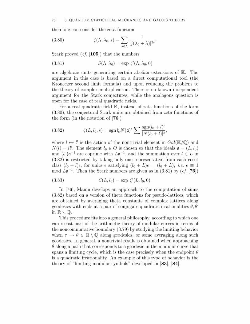
78 3. QUANTUM STATISTICAL MECHANICS AND GALOIS THEORY
then one can consider the zeta function
(3.80) ζ(Λ, λ0, s) =∑
λ∈Λ
1
|j(λ0 + λ)|2s.
Stark proved (cf. [105]) that the numbers
(3.81) S(Λ, λ0) = exp ζ ′(Λ, λ0, 0)
are algebraic units generating certain abelian extensions of K. Theargument in this case is based on a direct computational tool (theKronecker second limit formula) and upon reducing the problem tothe theory of complex multiplication. There is no known independentargument for the Stark conjectures, while the analogous question isopen for the case of real quadratic fields.
For a real quadratic field K, instead of zeta functions of the form(3.80), the conjectural Stark units are obtained from zeta functions ofthe form (in the notation of [76])
(3.82) ζ(L, l0, s) = sgn l′0N(a)s∑ sgn(l0 + l)′
|N(l0 + l)|s ,
where l 7→ l′ is the action of the nontrivial element in Gal(K/Q) andN(l) = ll′. The element l0 ∈ O is chosen so that the ideals a = (L, l0)and (l0)a
−1 are coprime with La−1, and the summation over l ∈ L in(3.82) is restricted by taking only one representative from each cosetclass (l0 + l)ε, for units ε satisfying (l0 + L)ε = (l0 + L), i.e. ε ≡ 1mod La−1. Then the Stark numbers are given as in (3.81) by (cf. [76])
(3.83) S(L, l0) = exp ζ ′(L, l0, 0).
In [76], Manin develops an approach to the computation of sums(3.82) based on a version of theta functions for pseudo-lattices, whichare obtained by averaging theta constants of complex lattices alonggeodesics with ends at a pair of conjugate quadratic irrationalities θ, θ′
in R r Q.This procedure fits into a general philosophy, according to which one
can recast part of the arithmetic theory of modular curves in terms ofthe noncommutative boundary (3.79) by studying the limiting behaviorwhen τ → θ ∈ R \ Q along geodesics, or some averaging along suchgeodesics. In general, a nontrivial result is obtained when approachingθ along a path that corresponds to a geodesic in the modular curve thatspans a limiting cycle, which is the case precisely when the endpoint θis a quadratic irrationality. An example of this type of behavior is thetheory of “limiting modular symbols” developed in [83], [84].
5. QUADRATIC FIELDS 79
5.3. Pseudolattices and the GL2-system. The noncommuta-tive space (3.35) of the GL2-system also admits a compactification,now given by adding the boundary P1(R) to H±, as in the noncommu-tative compactification of modular curves of [83],
(3.84)Sh(nc)(GL2, H
±) := GL2(Q)\(M2(Af)× P1(C))
= GL2(Q)\M2(A)/C∗,
where P1(C) = H± ∪ P1(R).This corresponds to adding to the space of commensurability classes
of 2-dimensional Q-lattices the pseudolattices in the sense of [76], hereconsidered together with a Q-structure. It seems then that Manin’sreal multiplication program may fit in with the boundary of the non-commutative space of the GL2-system. The crucial question in thisrespect becomes the construction of an arithmetic algebra associatedto the noncommutative modular curves. The results illustrated in theprevious chapter, regarding identities involving modular forms at theboundary of the classical modular curves and limiting modular sym-bols, as well as the still mysterious phenomenon of “quantum modularforms” identified by Zagier, point to the fact that there should exista rich class of objects replacing modular forms, when “pushed to theboundary”.
Regarding the role of modular forms, notice that, in the case of(3.84), we can again consider the dual system. This is a C∗-bundle
(3.85) L2 = GL2(Q)\M2(A).
On this dual space modular forms appear naturally instead of modularfunctions and the algebra of coordinates contains the modular Heckealgebra of Connes–Moscovici ([41], [42]) as arithmetic subalgebra.
Thus, the noncommutative geometry of the space of Q-lattices mod-ulo the equivalence relation of commensurability provides a setting thatunifies several phenomena involving the interaction of noncommutativegeometry and number theory. These include the Bost–Connes system,the noncommutative space underlying the construction of the spec-tral realization of the zeros of the Riemann zeta function in [23], themodular Hecke algebras of [41] [42], and the noncommutative modularcurves of [83].

CHAPTER 4
Noncommutative geometry at arithmetic infinity
This chapter is based on joint work of Katia Consani and the au-thor ([44], [45], [46], [47], [48]) that proposes a model for the dualgraph of the maximally degenerate fibers at the archimedean placesof an arithmetic surface in terms of a noncommutative space (spec-tral triple) related to the action of a Schottky group on its limit set.This description of∞-adic geometry provides a compatible setting thatcombines Manin’s result [79] on the Arakelov Green function for arith-metic surfaces in terms of hyperbolic geometry and for a cohomologi-cal construction of Consani [43] associated to the archimedean fibersof arithmetic varieties, related to Deninger’s calculation of the localL-factors as regularized determinants (cf. [52], [53]).
1. Schottky uniformization
Topologically a compact Riemann surface X of genus g is obtainedby gluing the sides of a 4g-gon. Correspondingly, the fundamentalgroup has a presentation
π1(X) = 〈a1, . . . , ag, b1, . . . , bg |∏
i
[ai, bi] = 1〉,
where the generators ai and bi label the sides of the polygon.In the genus g = 1 case, the parallelogram is the fundamental do-
main of the π1(X) ' Z2 action on the plane C, so that X = C/(Z+Zτ)is an elliptic curve.
For genus at least g ≥ 2, the hyperbolic plane H2 admits a tessel-lation by regular 4g-gons, and the action of the fundamental group bydeck transformations is realized by the action of a subgroup π1(X) 'G ⊂ PSL(2, R) by isometries of H2. This endows the compact Riemannsurface X with a hyperbolic metric and a Fuchsian uniformization
X = G\H2.
Another, less well known, type of uniformization of compact Rie-mann surfaces is Schottky uniformization. We recall briefly some gen-eral facts on Schottky groups.
81
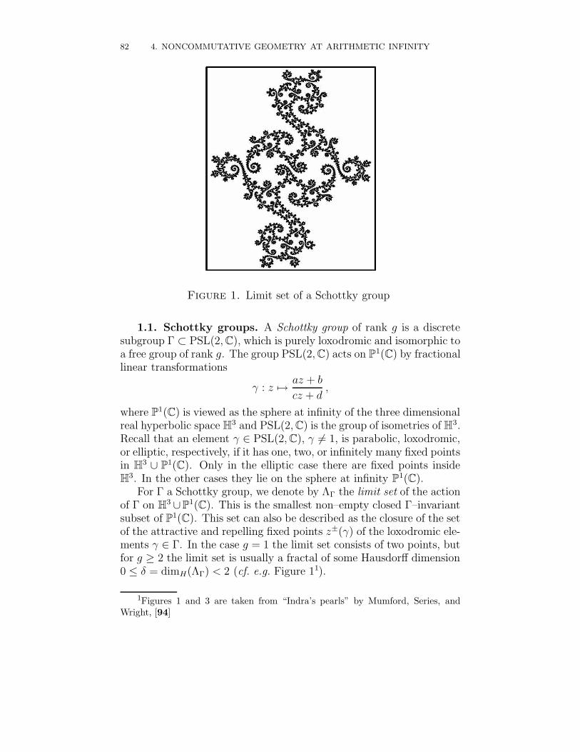
82 4. NONCOMMUTATIVE GEOMETRY AT ARITHMETIC INFINITY
Figure 1. Limit set of a Schottky group
1.1. Schottky groups. A Schottky group of rank g is a discretesubgroup Γ ⊂ PSL(2, C), which is purely loxodromic and isomorphic toa free group of rank g. The group PSL(2, C) acts on P1(C) by fractionallinear transformations
γ : z 7→ az + b
cz + d,
where P1(C) is viewed as the sphere at infinity of the three dimensionalreal hyperbolic space H3 and PSL(2, C) is the group of isometries of H3.Recall that an element γ ∈ PSL(2, C), γ 6= 1, is parabolic, loxodromic,or elliptic, respectively, if it has one, two, or infinitely many fixed pointsin H3 ∪ P1(C). Only in the elliptic case there are fixed points insideH3. In the other cases they lie on the sphere at infinity P1(C).
For Γ a Schottky group, we denote by ΛΓ the limit set of the actionof Γ on H3 ∪P1(C). This is the smallest non–empty closed Γ–invariantsubset of P1(C). This set can also be described as the closure of the setof the attractive and repelling fixed points z±(γ) of the loxodromic ele-ments γ ∈ Γ. In the case g = 1 the limit set consists of two points, butfor g ≥ 2 the limit set is usually a fractal of some Hausdorff dimension0 ≤ δ = dimH(ΛΓ) < 2 (cf. e.g. Figure 11).
1Figures 1 and 3 are taken from “Indra’s pearls” by Mumford, Series, andWright, [94]
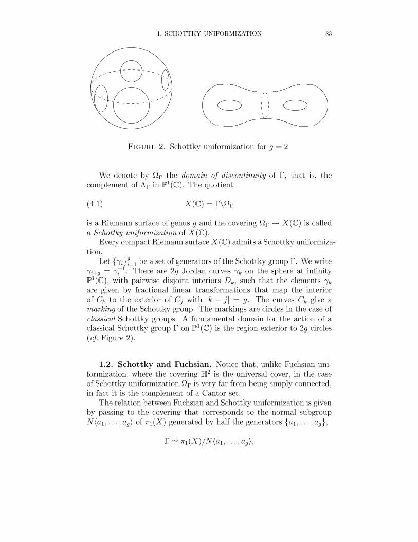
1. SCHOTTKY UNIFORMIZATION 83
Figure 2. Schottky uniformization for g = 2
We denote by ΩΓ the domain of discontinuity of Γ, that is, thecomplement of ΛΓ in P1(C). The quotient
(4.1) X(C) = Γ\ΩΓ
is a Riemann surface of genus g and the covering ΩΓ → X(C) is calleda Schottky uniformization of X(C).
Every compact Riemann surface X(C) admits a Schottky uniformiza-tion.
Let γigi=1 be a set of generators of the Schottky group Γ. We writeγi+g = γ−1
i . There are 2g Jordan curves γk on the sphere at infinityP1(C), with pairwise disjoint interiors Dk, such that the elements γk
are given by fractional linear transformations that map the interiorof Ck to the exterior of Cj with |k − j| = g. The curves Ck give amarking of the Schottky group. The markings are circles in the case ofclassical Schottky groups. A fundamental domain for the action of aclassical Schottky group Γ on P1(C) is the region exterior to 2g circles(cf. Figure 2).
1.2. Schottky and Fuchsian. Notice that, unlike Fuchsian uni-formization, where the covering H2 is the universal cover, in the caseof Schottky uniformization ΩΓ is very far from being simply connected,in fact it is the complement of a Cantor set.
The relation between Fuchsian and Schottky uniformization is givenby passing to the covering that corresponds to the normal subgroupN〈a1, . . . , ag〉 of π1(X) generated by half the generators a1, . . . , ag,
Γ ' π1(X)/N〈a1, . . . , ag〉,
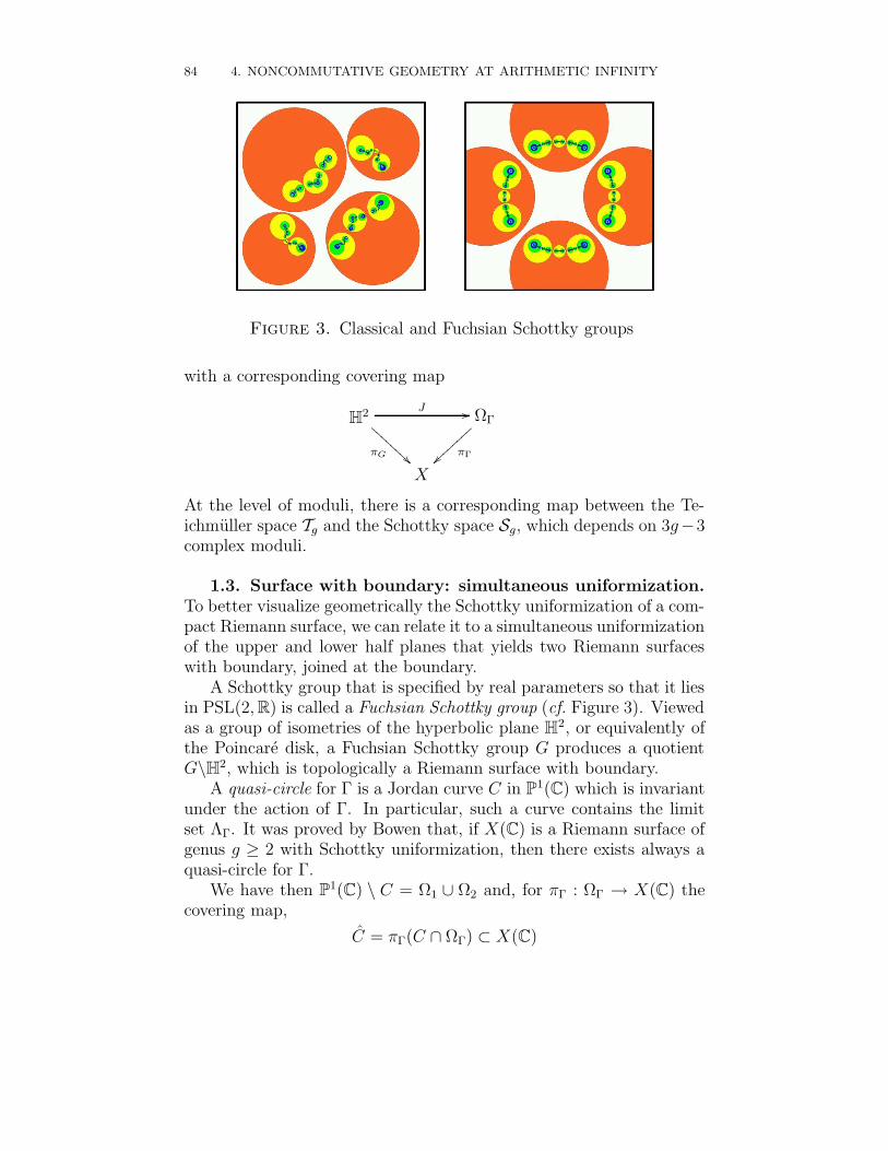
84 4. NONCOMMUTATIVE GEOMETRY AT ARITHMETIC INFINITY
Figure 3. Classical and Fuchsian Schottky groups
with a corresponding covering map
H2 J //
πG AAA
AAAA
AΩΓ
πΓ~~
X
At the level of moduli, there is a corresponding map between the Te-ichmuller space Tg and the Schottky space Sg, which depends on 3g−3complex moduli.
1.3. Surface with boundary: simultaneous uniformization.
To better visualize geometrically the Schottky uniformization of a com-pact Riemann surface, we can relate it to a simultaneous uniformizationof the upper and lower half planes that yields two Riemann surfaceswith boundary, joined at the boundary.
A Schottky group that is specified by real parameters so that it liesin PSL(2, R) is called a Fuchsian Schottky group (cf. Figure 3). Viewedas a group of isometries of the hyperbolic plane H2, or equivalently ofthe Poincare disk, a Fuchsian Schottky group G produces a quotientG\H2, which is topologically a Riemann surface with boundary.
A quasi-circle for Γ is a Jordan curve C in P1(C) which is invariantunder the action of Γ. In particular, such a curve contains the limitset ΛΓ. It was proved by Bowen that, if X(C) is a Riemann surface ofgenus g ≥ 2 with Schottky uniformization, then there exists always aquasi-circle for Γ.
We have then P1(C) \ C = Ω1 ∪ Ω2 and, for πΓ : ΩΓ → X(C) thecovering map,
C = πΓ(C ∩ ΩΓ) ⊂ X(C)
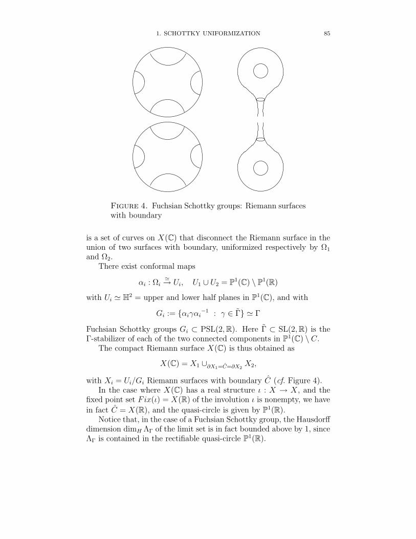
1. SCHOTTKY UNIFORMIZATION 85
Figure 4. Fuchsian Schottky groups: Riemann surfaceswith boundary
is a set of curves on X(C) that disconnect the Riemann surface in theunion of two surfaces with boundary, uniformized respectively by Ω1
and Ω2.There exist conformal maps
αi : Ωi'→ Ui, U1 ∪ U2 = P1(C) \ P1(R)
with Ui ' H2 = upper and lower half planes in P1(C), and with
Gi := αiγαi−1 : γ ∈ Γ ' Γ
Fuchsian Schottky groups Gi ⊂ PSL(2, R). Here Γ ⊂ SL(2, R) is theΓ-stabilizer of each of the two connected components in P1(C) \ C.
The compact Riemann surface X(C) is thus obtained as
X(C) = X1 ∪∂X1=C=∂X2X2,
with Xi = Ui/Gi Riemann surfaces with boundary C (cf. Figure 4).In the case where X(C) has a real structure ι : X → X, and the
fixed point set Fix(ι) = X(R) of the involution ι is nonempty, we have
in fact C = X(R), and the quasi-circle is given by P1(R).Notice that, in the case of a Fuchsian Schottky group, the Hausdorff
dimension dimH ΛΓ of the limit set is in fact bounded above by 1, sinceΛΓ is contained in the rectifiable quasi-circle P1(R).
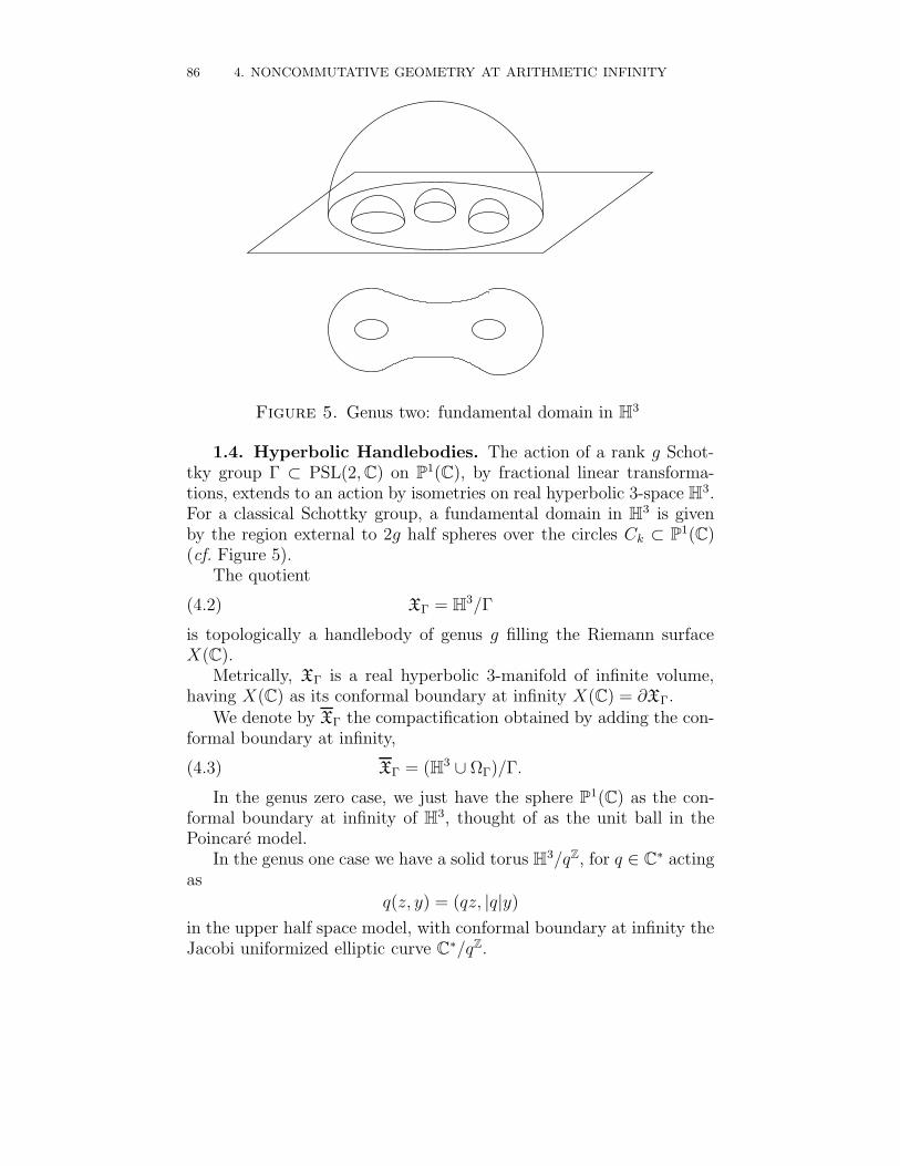
86 4. NONCOMMUTATIVE GEOMETRY AT ARITHMETIC INFINITY
Figure 5. Genus two: fundamental domain in H3
1.4. Hyperbolic Handlebodies. The action of a rank g Schot-tky group Γ ⊂ PSL(2, C) on P1(C), by fractional linear transforma-tions, extends to an action by isometries on real hyperbolic 3-space H3.For a classical Schottky group, a fundamental domain in H3 is givenby the region external to 2g half spheres over the circles Ck ⊂ P1(C)(cf. Figure 5).
The quotient
(4.2) XΓ = H3/Γ
is topologically a handlebody of genus g filling the Riemann surfaceX(C).
Metrically, XΓ is a real hyperbolic 3-manifold of infinite volume,having X(C) as its conformal boundary at infinity X(C) = ∂XΓ.
We denote by XΓ the compactification obtained by adding the con-formal boundary at infinity,
(4.3) XΓ = (H3 ∪ ΩΓ)/Γ.
In the genus zero case, we just have the sphere P1(C) as the con-formal boundary at infinity of H3, thought of as the unit ball in thePoincare model.
In the genus one case we have a solid torus H3/qZ, for q ∈ C∗ actingas
q(z, y) = (qz, |q|y)
in the upper half space model, with conformal boundary at infinity theJacobi uniformized elliptic curve C∗/qZ.
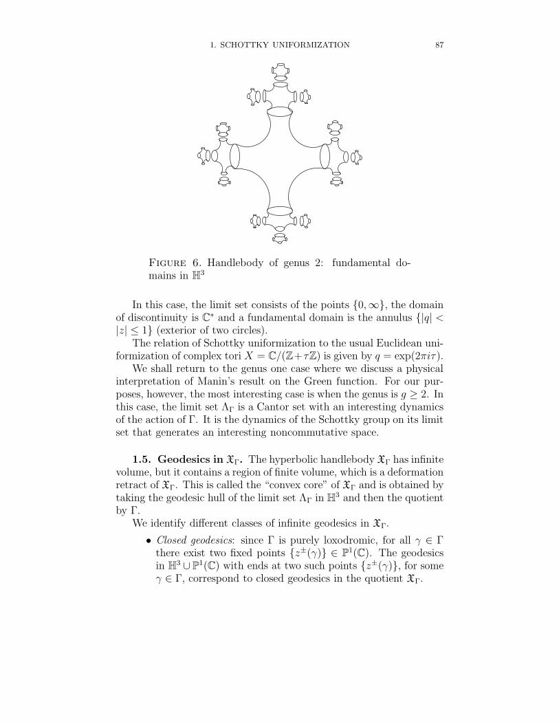
1. SCHOTTKY UNIFORMIZATION 87
Figure 6. Handlebody of genus 2: fundamental do-mains in H3
In this case, the limit set consists of the points 0,∞, the domainof discontinuity is C∗ and a fundamental domain is the annulus |q| <|z| ≤ 1 (exterior of two circles).
The relation of Schottky uniformization to the usual Euclidean uni-formization of complex tori X = C/(Z+τZ) is given by q = exp(2πiτ).
We shall return to the genus one case where we discuss a physicalinterpretation of Manin’s result on the Green function. For our pur-poses, however, the most interesting case is when the genus is g ≥ 2. Inthis case, the limit set ΛΓ is a Cantor set with an interesting dynamicsof the action of Γ. It is the dynamics of the Schottky group on its limitset that generates an interesting noncommutative space.
1.5. Geodesics in XΓ. The hyperbolic handlebody XΓ has infinitevolume, but it contains a region of finite volume, which is a deformationretract of XΓ. This is called the “convex core” of XΓ and is obtained bytaking the geodesic hull of the limit set ΛΓ in H3 and then the quotientby Γ.
We identify different classes of infinite geodesics in XΓ.
• Closed geodesics: since Γ is purely loxodromic, for all γ ∈ Γthere exist two fixed points z±(γ) ∈ P1(C). The geodesicsin H3 ∪ P1(C) with ends at two such points z±(γ), for someγ ∈ Γ, correspond to closed geodesics in the quotient XΓ.
88 4. NONCOMMUTATIVE GEOMETRY AT ARITHMETIC INFINITY
• Bounded geodesics: The images in XΓ of geodesics in H3∪P1(C)having both ends on the limit set ΛΓ are geodesics that remainconfined within the convex core of XΓ.
• Unbounded geodesics: these are the geodesics in XΓ that even-tually wander off the convex core towards the conformal bound-ary X(C) at infinity. They correspond to geodesics in H3 ∪P1(C) with at least one end at a point of ΩΓ.
In the genus one case, there is a unique primitive closed geodesic,namely the image in the quotient of the geodesic in H3 connecting 0and ∞. The bounded geodesics are those corresponding to geodesicsin H3 originating at 0 or ∞.
The most interesting case is that of genus g ≥ 2, where the boundedgeodesics form a complicated tangle inside XΓ. Topologically, this isa generalized solenoid, namely it is locally the product of a line and aCantor set.
2. Dynamics and noncommutative geometry
Since the uniformizing group Γ is a free group, there is a simple wayof obtaining a coding of the bounded geodesics in XΓ. The set of suchgeodesics can be identified with ΛΓ×Γ ΛΓ, by specifying the endpointsin H3 ∪ P1(C) modulo the action of Γ.
If γigi=1 is a choice of generators of Γ and γi+g = γ−1i , i = 1, . . . , g,
we can introduce a subshift of finite type (S, T ) where(4.4)S = . . . a−m . . . a−1a0a1 . . . a` . . . |ai ∈ γi2g
i=1, ai+1 6= a−1i , ∀i ∈ Z
is the set of doubly infinite words in the generators and their inverses,with the admissibility condition that no cancellations occur. The mapT is the invertible shift
(4.5) T (. . . a−m . . . a−1a0a1 . . . a` . . .) = . . . a−m+1 . . . a0a1a2 . . . a`+1 . . .
Then we can pass from the discrete dynamical system (S, T ) to itssuspension flow and obtain the mapping torus
(4.6) ST := S × [0, 1]/(x, 0) ∼ (Tx, 1).
Topologically this space is a solenoid, that is, a bundle over S1 withfiber a Cantor set.
2.1. Homotopy quotient. The space ST of (4.6) has a naturalinterpretation in noncommutative geometry as the homotopy quotient
2. DYNAMICS AND NONCOMMUTATIVE GEOMETRY 89
in the sense of Baum–Connes [7] of the noncommutative space givenby the C∗-algebra
(4.7) C(S) oT Z
describing the action of the shift (4.5) on the totally disconnectedspace (4.4). The noncommutative space (4.7) parameterizes boundedgeodesics in the handlebody XΓ.
The homotopy quotient is given by
S ×Z R = ST .
The K-theory of the C∗-algebra (4.7) can be computed via thePimsner–Voiculescu six terms exact sequence,
K1(A) // K0(C(S))δ=1−T// K0(C(S))
K1(C(S))
OO
K1(C(S))oo K0(A)oo
where A = C(S) oT Z. Here, since the space S is totally disconnected,we have K1(C(S)) = 0 and K0(C(S)) = C(S, Z) (locally constantinteger valued functions). Thus the exact sequence becomes
(4.8) 0→ K1(A)→ C(S, Z)δ=1−T→ C(S, Z)→ K0(A)→ 0,
and we obtain K1(A) = Z = Ker(δ) and K0(A) = Coker(δ). In dy-namical systems language, these are respectively the invariants andcoinvariants of the invertible shift T (cf. [11] [95]).
In terms of the homotopy quotient, one can describe this exactsequence more geometrically in terms of the Thom isomorphism andthe µ-map
µ : K∗+1(ST ) ∼= H∗+1(ST , Z)→ K∗(C(S) oT Z).
Thus, we obtain:
K1(A) ' H0(ST ) = Z
K0(A) ' H1(ST )
The H1(ST ) can be identified with the Cech cohomology group givenby the homotopy classes [ST , U(1)], by mapping f 7→ [exp(2πitf(x))],for f ∈ C(S, Z)/δ(C(S, Z)).
90 4. NONCOMMUTATIVE GEOMETRY AT ARITHMETIC INFINITY
2.2. Filtration. The identification
H1(ST , Z) ∼= K0(C(S) oT Z)
of the cohomology of ST with the K0-group of the crossed product C∗-algebra for the action of T on S endows H1(ST , Z) with a filtration.
Theorem 2.1. The first cohomology of ST is a direct limit
H1(ST ) = lim−→n
Fn,
of free abelian groups F0 → F1 → · · ·Fn → · · · of ranks rank F0 = 2gand rank Fn = 2g(2g − 1)n−1(2g − 2) + 1, for n ≥ 1.
In fact, by the Pimsner-Voiculescu six terms exact sequence, thegroup K0(C(S) oT Z) can be identified with the cokernel of the map1− T acting as f 7→ f − f T on the Z module C(S, Z) ' K0(C(S)).
Then the filtration is given by the submodules of functions depend-ing only on the a0 . . . an coordinates in the doubly infinite words de-scribing points in S. Namely, one first shows that
H1(ST , Z) = C(S, Z)/δ(C(S, Z)) = P/δPwhere P denotes the Z-module of locally constant Z-valued functionsthat depend only on “future coordinates”. This can be identified withfunctions on the limit set ΛΓ, since each point in ΛΓ is described byan infinite (to the right) admissible sequence in the generators γi andtheir inverses. We have P ' C(ΛΓ, Z).
The module P clearly has a filtration by the submodules Pn offunctions of the first n + 1 coordinates. These have
rankPn = 2g(2g − 1)n.
We set Fn := Pn/δPn−1. One can show that there are inducedinjections Fn → Fn+1 and that
H1(ST ) = lim−→n
Fn.
Moreover, we have rankFn = θn− θn−1 + 1, where θn is the numberof admissible words of length n + 1. All the Z modules Fn and thequotients Fn/Fn−1 are torsion free (cf. [95]).
2.3. Hilbert space and grading. It is convenient to consider thecomplex vector space
PC = C(ΛΓ, Z)⊗ C
2. DYNAMICS AND NONCOMMUTATIVE GEOMETRY 91
and the corresponding exact sequence computing the cohomology withC coefficients:
(4.9) 0→ C→ PCδ−→ PC → H1(ST , C)→ 0
The complex vector space PC sits in the Hilbert space
PC ⊂ L = L2(ΛΓ, dµ),
where µ is the Patterson–Sullivan measure on the limit set, satisfying
γ∗dµ = |γ′|dimH(ΛΓ)dµ,
with dimH(ΛΓ) the Hausdorff dimension.This gives a Hilbert space L, together with a filtration Pn by finite
dimensional subspaces. In such a setting, it is natural to consider acorresponding grading operator,
(4.10) D =∑
n
nΠn,
where Πn denotes the orthogonal projection onto Pn and Πn = Πn −Πn−1.
2.4. Cuntz–Krieger algebra. There is a noncommutative spacethat encodes nicely the dynamics of the Schottky group Γ on its limitset ΛΓ. Consider the 2g × 2g matrix A that gives the admissibilitycondition for sequences in S: this is the matrix with 0, 1 entriessatisfying Aij = 1 for |i− j| 6= g and Aij = 0 otherwise.
The Cuntz–Krieger algebra OA associated to this matrix is the uni-versal C∗-algebra generated by partial isometries Si, i = 1, . . . , 2g,satisfying the relations
∑
j
SjS∗j = 1 S∗
i Si =∑
j
AijSjS∗j .
Recall that a partial isometry is an operator S satisfying S = SS∗S.This algebra is related to the Schottky group by the following result.
Proposition 2.2. There is an isomorphism
(4.11) OA∼= C(ΛΓ) o Γ.
Up to a stabilization (tensoring with compact operators), the alge-bra has another crossed product description as
(4.12) OA ' FA oT Z,
with FA an AF-algebra (a direct limit of finite dimensional C∗-algebras).Consider the cochain complex of Hilbert spaces
0→ C→ L δ→ L→ H→ 0
92 4. NONCOMMUTATIVE GEOMETRY AT ARITHMETIC INFINITY
determined by the Pimsner–Voiculescu sequence (4.8).
Proposition 2.3. The C∗-algebra OA admits a faithful represen-tation on the Hilbert space L = L2(ΛΓ, dµ).
This is obtained as follows.For dH = dimH(ΛΓ) the Hausdorff dimension, consider the opera-
tors
(4.13) Pi f = χγif Ti f = |(γ−1
i )′|dH/2 f γ−1i ,
where γi are the generators of Γ and their inverses and
(4.14) Tγ f = |γ′|dH/2f γ.
Then the operators
(4.15) Si =∑
j
AijT∗i Pj
are partial isometries on L satisfying the Cuntz–Krieger relations forthe matrix A of the subshift of finite type (4.4). This gives the repre-sentation of OA.
2.5. Spectral triple for Schottky groups. On the Hilbert spaceH = L⊕L consider the diagonal action of the algebra OA and the Diracoperator D defined as
(4.16)D|L⊕0 =
∑n (n + 1) (Πn ⊕ 0)
D|0⊕L = −∑n n (0⊕ Πn).
The choice of the sign in (4.16) is not optimal from the point ofview of the K-homology class. A better choice would be
F =
(0 11 0
).
This would require in turn a modification of |D|. A construction alongthese lines is being considered in joint work of the author with AlinaVdovina and Gunther Cornelissen. In our setting here, the reasonfor the choice (4.16) in [44] is the formula (4.91) relating D to the“logarithm of Frobenius” at arithmetic infinity.
Theorem 2.4. For a Schottky group Γ with dimH(ΛΓ) < 1, thedata (OA,H,D), for H = L⊕L with the diagonal action of OA throughthe representation (4.15) and the Dirac operator (4.16), define a non-finitely summable, θ-summable spectral triple.
3. ARITHMETIC INFINITY: ARCHIMEDEAN PRIMES 93
The key point of this result is the compatibility relation between thealgebra and the Dirac operator, namely the fact that the commutators[D, a] are bounded operators, for all a ∈ Oalg
A , the involutive subal-gebra generated algebraically by the Si subject to the Cuntz–Kriegerrelations.
This follows by an estimate on the norm of the commutators ‖[D, Si]‖and ‖[D, S∗
i ]‖, in terms of the Poincare series of the Schottky group(dH < 1) ∑
γ∈Γ
|γ ′|s, s = 1 > dH ,
where the Hausdorff dimension dH is the exponent of convergence ofthe Poincare series.
The dimension of the n-th eigenspace of D is 2g(2g− 1)n−1(2g− 2)for n ≥ 1, 2g for n = 0 and 2g(2g − 1)−n−1(2g − 2) for n ≤ −1, so thespectral triple is not finitely summable, since |D|z is not of trace class.It is θ summable, since the operator exp(−tD2) is of trace class, for allt > 0.
Using the description (4.12) of the noncommutative space as crossedproduct of an AF algebra by the action of the shift, FA oT Z, one maybe able to find a 1-summable spectral triple. Here the dense subalgebrashould not contain any of the group elements. In fact, by the result of[20], the group Γ is a free group, hence its growth is too fast to supportfinitely summable spectral triples on its group ring.
3. Arithmetic infinity: archimedean primes
An algebraic number field K, which is an extension of Q such that[K : Q] = n, admits n = r1 + 2r2 embeddings
(4.17) α : K → C.
These can be subdivided into r1 real embeddings K → R and r2 pairs ofcomplex conjugate embeddings. The embeddings (4.17) are called thearchimedean primes of the number field. The set of archimedean primesis often referred to as “arithmetic infinity”, a terminology borrowedfrom the case of the unique embedding of Q → R, which is called the“infinite prime”.
A general strategy in arithmetic geometry is to adapt the tools ofclassical algebraic geometry to the arithmetic setting. In particular,over Q the set of primes Spec(Z) is the analog in arithmetic geometryof the affine line. It becomes clear then that some compactification isnecessary, at least in order to have a well behaved form of intersec-tion theory in arithmetic geometry. Namely, we need to pass from the
94 4. NONCOMMUTATIVE GEOMETRY AT ARITHMETIC INFINITY
“affine” Spec(Z) to the projective case. The compactification is ob-tained by adding the infinite prime to the set of finite primes. A goalof arithmetic geometry then becomes developing a setting that treatsthe infinite prime and the finite primes of equal footing.
More generally, for a number field K with OK its ring of inte-gers, the set of primes Spec(OK) is compactified by adding the setof “archimedean primes”
(4.18) Spec(OK) = Spec(OK) ∪ α : K → C.
3.1. Arithmetic surfaces. Let X be a smooth projective alge-braic curve defined over Q. Then, by clearing denominators one ob-tains an equation with Z coefficients. This determines a scheme XZ
over Spec(Z),
XZ ⊗Z Spec(Q) = X,
where the closed fiber of XZ at a prime p ∈ Spec(Z) is the reduction ofX mod p. Thus, viewed as an arithmetic variety, an algebraic curvebecomes a 2-dimensional fibration over the affine line Spec(Z).
One can also consider reductions of X (defined over Z) modulopn for some prime p ∈ Spec(Z). The limit as n → ∞ defines a p–adic completion of XZ. This can be thought of as an “infinitesimalneighborhood” of the fiber at p.
The picture is more complicated at arithmetic infinity, since onedoes not have a suitable notion of “reduction mod ∞” available todefine the closed fiber. On the other hand, one does have the analog ofthe p–adic completion at hand. This is given by the Riemann surface(smooth projective algebraic curve over C) determined by the equationof the algebraic curve X over Q, under the embedding of Q ⊂ C,
X(C) = X ⊗Q Spec(C)
with the absolute value | · | at the infinite prime replacing the p-adicvaluations.
Similarly, for K a number field and OK its ring of integers, a smoothproper algebraic curve X over K determines a smooth minimal modelXOK
, which defines an arithmetic surface XOKover Spec(OK). The
closed fiber X℘ of XOKover a prime ℘ ∈ OK is given by the reduction
mod ℘.When Spec(OK) is compactified by adding the archimedean primes,
one also obtains n Riemann surfaces Xα(C), obtained from the equationdefining X over K under the embeddings α : K → C. Of these Riemannsurfaces, r1 carry a real involution.
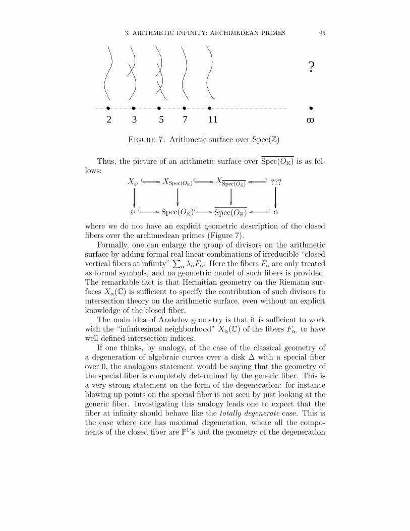
3. ARITHMETIC INFINITY: ARCHIMEDEAN PRIMES 95
?
117532 oo
Figure 7. Arithmetic surface over Spec(Z)
Thus, the picture of an arithmetic surface over Spec(OK) is as fol-lows:
X℘
// XSpec(OK)
// XSpec(OK)
???? _oo
℘ // Spec(OK) // Spec(OK) α? _oo
where we do not have an explicit geometric description of the closedfibers over the archimedean primes (Figure 7).
Formally, one can enlarge the group of divisors on the arithmeticsurface by adding formal real linear combinations of irreducible “closedvertical fibers at infinity”
∑α λαFα. Here the fibers Fα are only treated
as formal symbols, and no geometric model of such fibers is provided.The remarkable fact is that Hermitian geometry on the Riemann sur-faces Xα(C) is sufficient to specify the contribution of such divisors tointersection theory on the arithmetic surface, even without an explicitknowledge of the closed fiber.
The main idea of Arakelov geometry is that it is sufficient to workwith the “infinitesimal neighborhood” Xα(C) of the fibers Fα, to havewell defined intersection indices.
If one thinks, by analogy, of the case of the classical geometry ofa degeneration of algebraic curves over a disk ∆ with a special fiberover 0, the analogous statement would be saying that the geometry ofthe special fiber is completely determined by the generic fiber. This isa very strong statement on the form of the degeneration: for instanceblowing up points on the special fiber is not seen by just looking at thegeneric fiber. Investigating this analogy leads one to expect that thefiber at infinity should behave like the totally degenerate case. This isthe case where one has maximal degeneration, where all the compo-nents of the closed fiber are P1’s and the geometry of the degeneration
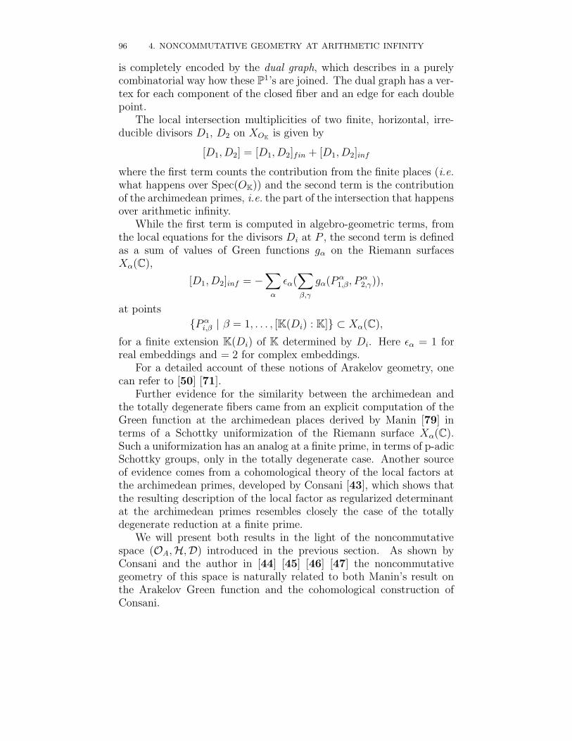
96 4. NONCOMMUTATIVE GEOMETRY AT ARITHMETIC INFINITY
is completely encoded by the dual graph, which describes in a purelycombinatorial way how these P1’s are joined. The dual graph has a ver-tex for each component of the closed fiber and an edge for each doublepoint.
The local intersection multiplicities of two finite, horizontal, irre-ducible divisors D1, D2 on XOK
is given by
[D1, D2] = [D1, D2]fin + [D1, D2]inf
where the first term counts the contribution from the finite places (i.e.what happens over Spec(OK)) and the second term is the contributionof the archimedean primes, i.e. the part of the intersection that happensover arithmetic infinity.
While the first term is computed in algebro-geometric terms, fromthe local equations for the divisors Di at P , the second term is definedas a sum of values of Green functions gα on the Riemann surfacesXα(C),
[D1, D2]inf = −∑
α
εα(∑
β,γ
gα(P α1,β, P α
2,γ)),
at points
P αi,β | β = 1, . . . , [K(Di) : K] ⊂ Xα(C),
for a finite extension K(Di) of K determined by Di. Here εα = 1 forreal embeddings and = 2 for complex embeddings.
For a detailed account of these notions of Arakelov geometry, onecan refer to [50] [71].
Further evidence for the similarity between the archimedean andthe totally degenerate fibers came from an explicit computation of theGreen function at the archimedean places derived by Manin [79] interms of a Schottky uniformization of the Riemann surface Xα(C).Such a uniformization has an analog at a finite prime, in terms of p-adicSchottky groups, only in the totally degenerate case. Another sourceof evidence comes from a cohomological theory of the local factors atthe archimedean primes, developed by Consani [43], which shows thatthe resulting description of the local factor as regularized determinantat the archimedean primes resembles closely the case of the totallydegenerate reduction at a finite prime.
We will present both results in the light of the noncommutativespace (OA,H,D) introduced in the previous section. As shown byConsani and the author in [44] [45] [46] [47] the noncommutativegeometry of this space is naturally related to both Manin’s result onthe Arakelov Green function and the cohomological construction ofConsani.
4. ARAKELOV GEOMETRY AND HYPERBOLIC GEOMETRY 97
4. Arakelov geometry and hyperbolic geometry
In this section we give a detailed account of Manin’s result [79] onthe relation between the Arakelov Green function on a Riemann surfaceX(C) with Schottky uniformization and geodesics in the 3-dimensionalhyperbolic handlebody XΓ. Our exposition follows closely the seminalpaper [79].
4.1. Arakelov Green function. Given a divisor A =∑
x mx(x)with support |A| on a smooth compact Riemann surface X(C), anda choice of a positive real–analytic 2-form dµ on X(C), the Greenfunction gµ,A = gA is a real analytic function on on X(C)\|A|, uniquelydetermined by the following conditions:
• Laplace equation: gA satisfies ∂∂ gA = πi (deg(A) dµ − δA),with δA the δ–current ϕ 7→∑
x mxϕ(x).
• Singularities: if z is a local coordinate in a neighborhood of x,then gA −mx log |z| is locally real analytic.
• Normalization: gA satisfies∫
XgAdµ = 0.
If B =∑
y ny(y) is another divisor, such that |A| ∩ |B| = ∅, then
the expression gµ(A, B) :=∑
y nygµ,A(y) is symmetric and biadditivein A, B. Generally, such an expression gµ depends on µ, where thechoice of µ is equivalent to the choice of a real analytic Riemannianmetric on X(C), compatible with the complex structure.
However, in the special case of degree zero divisors, deg A = deg B =0, the gµ(A, B) = g(A, B) are conformal invariants.
In the case on the Riemann sphere P1(C), if wA is a meromorphicfunction with Div(wA) = A, we have
(4.19) g(A, B) = log∏
y∈|B|
|wA(y)|ny = Re
∫
γB
dwA
wA,
where γB is a 1–chain with boundary B.In the case of degree zero divisors A, B on a Riemann surface of
higher genus, the formula (4.19) can be generalized, replacing the loga-rithmic differential dwA/wA with a differential of the third kind (mero-morphic differential with nonvanishing residues) ωA with purely imag-inary periods and residues mx at x. This gives
(4.20) g(A, B) = Re
∫
γB
ωA.
Thus, one can explicitly compute g(A, B) from a basis of differen-tials of the third kind with purely imaginary periods.
98 4. NONCOMMUTATIVE GEOMETRY AT ARITHMETIC INFINITY
b*c,d
c,d
a*c,d
d
b
c
a
Figure 8. Cross ratio and geodesic length
4.2. Cross ratio and geodesics. The basic step leading to theresult of Manin, expressing the Arakelov Green function in terms ofgeodesics in the hyperbolic handlebody XΓ, is a very simple classicalfact of hyperbolic geometry, namely the fact that the cross ratio of fourpoints on P1(C) can be expressed in terms of geodesics in the ‘interior’H3:
(4.21) log |〈a, b, c, d〉| = −ordist (a ∗ c, d, b ∗ c, d) .
Here, following [79], ordist denotes the oriented distance, and we usethe notation a∗c, d to indicate the point on the geodesic c, d in H3
with endpoints c, d ∈ P1(C), obtained as the intersection of c, d withthe unique geodesic from a that cuts c, d at a right angle (Figure 8).
4.3. Differentials and Schottky uniformization. The next im-portant step in Manin’s result [79] is to show that, if X(C) = Γ\ΩΓ isa Riemann surface with a Schottky uniformization, then one obtains abasis of differentials of the third kind with purely imaginary periods,by taking suitable averages over the group Γ of expressions involvingthe cross ratio of points on P1(C).
We denote by C(|γ) a set of representatives of Γ/(γZ), by C(ρ|γ)a set of representatives for (ρZ) \ Γ/(γZ), and by S(γ) the conjugacyclass of γ in Γ.
Let wA be a meromorphic function on P1(C) with divisor A =(a)− (b), such that the support |A| is contained in the complement of
4. ARAKELOV GEOMETRY AND HYPERBOLIC GEOMETRY 99
an open neighborhood of ΛΓ. We use the notation
(4.22) 〈a, b, c, d〉 := (a− b)(c− d)
(a− d)(c− b)
for the cross-ratio of points a, b, c, d ∈ P1(C).For a fixed choice of a base point z0 ∈ ΩΓ, the series
(4.23) ν(a)−(b) :=∑
γ∈Γ
d log〈a, b, γz, γz0〉
gives the lift to ΩΓ of a differential of the third kind on the Riemann sur-face X(C), endowed with the choice of Schottky uniformization. Thesedifferentials have residues ±1 at the images of a and b in X(C), andthey have vanishing ak periods, where ak, bkk=1...g are the generatorsof the homology of X(C).
Similarly, we obtain lifts of differentials of the first kind on X(C),by considering the series
(4.24) ωγ =∑
h∈C(|γ)
d log〈hz+(γ), hz−(γ), z, z0〉,
where we denote by z+(γ), z−(γ) ⊂ ΛΓ the pair consisting of theattractive and repelling fixed points of γ ∈ Γ.
The series (4.23) and (4.24) converge absolutely on compact setsK ⊂ ΩΓ, whenever dimH ΛΓ < 1. Moreover, they do not depend onthe choice of the base point z0 ∈ ΩΓ.
In particular, given a choice γkgk=1 of generators of the Schottkygroup Γ, we obtain by (4.24) a basis of holomorphic differentials ωγk
,that satisfy
(4.25)
∫
ak
ωγ`= 2π
√−1 δk`.
One can then use a linear combination of the holomorphic differ-entials ωγk
to correct the meromorphic differentials ν(a)−(b) in such away that the resulting meromorphic differentials have purely imaginarybk–periods. Let X`(a, b) be coefficients such that the differentials of thethird kind
(4.26) ω(a)−(b) := ν(a)−(b) −∑
`
X`(a, b)ωg`
100 4. NONCOMMUTATIVE GEOMETRY AT ARITHMETIC INFINITY
have purely imaginary bk–periods. The coefficients X`(a, b) satisfy thesystem of equations(4.27)
g∑
`=1
X`(a, b)< (τkl) = <∫
bk
ν(a)−(b) =∑
h∈S(gk)
log |〈a, b, z+(h), z−(h)〉|.
Thus, one obtains ([79], cf. also [109]) from (4.20) and (4.26) thatthe Arakelov Green function for X(C) with Schottky uniformizationcan be computed as
(4.28)g((a)− (b), (c)− (d)) =
∑h∈Γ log |〈a, b, hc, hd〉|
−∑g`=1 X`(a, b)
∑h∈S(g`)
log |〈z+(h), z−(h), c, d〉|.Notice that this result seems to indicate that there is a choice of
Schottky uniformization involved as additional data for Arakelov ge-ometry at arithmetic infinity. However, as we remarked previously, atleast in the case of archimedean primes that are real embeddings (asis the case of arithmetic infinity for Q), the Schottky uniformizationis determined by the real structure, by splitting X(C) along the reallocus X(R), when the latter is nonempty.
4.4. Green function and geodesics. By combining the basicformula (4.21) with the formula (4.28) for the Green function on aRiemann surface with Schottky uniformization one can replace eachterm appearing in (4.28) with a corresponding term which computesthe oriented geodesic length of a certain arc of geodesic in XΓ:(4.29)
g((a)− (b), (c)− (d)) = −∑h∈Γ ordist(a ∗ hc, hd, b ∗ hc, hd)+∑g
`=1 X`(a, b)∑
h∈S(g`)ordist(z+(h) ∗ c, d, z−(h) ∗ c, d).
The coefficients X`(a, b) can also be expressed in terms of geodesics,using the equation (4.27).
5. Intermezzo: Quantum gravity and black holes
Anti-de Sitter space AdSd+1 is a highly symmetric space–time, sat-isfying Einstein’s equations with constant curvature R < 0. Physicallyit describes empty space with a negative cosmological constant. Inorder to avoid time–like closed geodesics, it is customary to pass to
the universal cover AdSd+1, whose boundary at infinity of the is a com-pactification of d–dimensional Minkowski space–time. When passing to
Euclidean signature, AdSd+1 becomes the real hyperbolic space Hd+1.
5. INTERMEZZO: QUANTUM GRAVITY AND BLACK HOLES 101
The (3 + 1)-dimensional Anti-de Sitter space is a well known ex-ample of space–time in general relativity. Topologically AdS3+1 isof the form S1 × R3, while metrically it is realized by the hyper-boloid −u2 − v2 + x2 + y2 + z2 = 1 in R5, with the metric elementds2 = −du2 − dv2 + dx2 + dy2 + dz2. The universal cover is topologi-cally R4. In the context of quantum gravity, it is especially interestingto consider the case of the (2 + 1)-dimensional Anti-de Sitter spaceAdS2+1 and its Euclidean counterpart, the real 3-dimensional hyper-bolic space H3.
The holographic principle postulates the existence of an explicitcorrespondence between gravity on a bulk space which is asymptotically
AdSd+1 (e.g. a space obtained as a global quotient of AdSd+1 by adiscrete group of isometries) and field theory on its conformal boundaryat infinity.
The relation (4.21), which identifies the Green function
g((a)− (b), (c)− (d))
on P1(C) with the oriented length of a geodesic arc in H3, can bethought of as an instance of this holography principle, when we in-terpret one side as geodesic propagator on the bulk space in a semi-classical approximation, and the other side (the Green function) asthe two-point correlation function of the boundary field theory. Noticethat, because of the prescribed behavior of the Green function at thesingularities given by the points of the divisor, our “four points” invari-ant g((a)− (b), (c)− (d)), when a→ c and b→ d, gives the two-pointcorrelator with a logarithmic divergence which is intrinsic and does notdepend on a choice of cut-off function (unlike the way regularization isoften used in the physics literature).
In [82] we showed that the relation (4.29) between Arakelov Greenfunctions and configurations of geodesics in the hyperbolic handlebody,proved by Manin in [79], provides in fact precisely the correspondenceprescribed by the holography principle, for a class of 2 + 1 dimen-sional space–times known as Euclidean Krasnov black holes. These in-clude the Banados–Teitelboim–Zanelli black holes: an important classof space–times in the context of (2 + 1)-dimensional quantum gravity.
5.1. Banados–Teitelboim–Zanelli black hole. We consider thecase of a hyperbolic handlebody of genus one (a solid torus), with con-formal boundary at infinity given by an elliptic curve.
Recall that we can describe elliptic curves via the Jacobi uniformiza-tion. (We have already encountered it in the previous lectures, in thecontext of non-commutative elliptic curves.) Let Xq(C) = C∗/qZ be
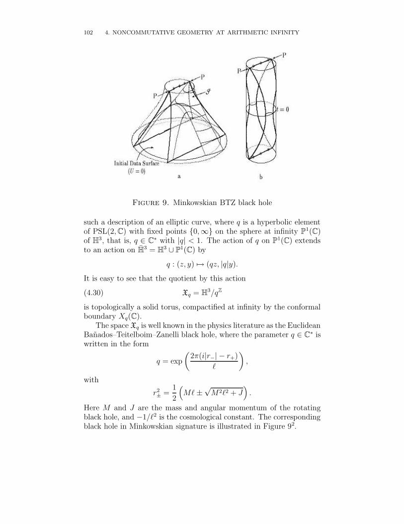
102 4. NONCOMMUTATIVE GEOMETRY AT ARITHMETIC INFINITY
Figure 9. Minkowskian BTZ black hole
such a description of an elliptic curve, where q is a hyperbolic elementof PSL(2, C) with fixed points 0,∞ on the sphere at infinity P1(C)of H3, that is, q ∈ C∗ with |q| < 1. The action of q on P1(C) extendsto an action on H3 = H3 ∪ P1(C) by
q : (z, y) 7→ (qz, |q|y).
It is easy to see that the quotient by this action
(4.30) Xq = H3/qZ
is topologically a solid torus, compactified at infinity by the conformalboundary Xq(C).
The space Xq is well known in the physics literature as the EuclideanBanados–Teitelboim–Zanelli black hole, where the parameter q ∈ C∗ iswritten in the form
q = exp
(2π(i|r−| − r+)
`
),
with
r2± =
1
2
(M`±
√M2`2 + J
).
Here M and J are the mass and angular momentum of the rotatingblack hole, and −1/`2 is the cosmological constant. The correspondingblack hole in Minkowskian signature is illustrated in Figure 92.
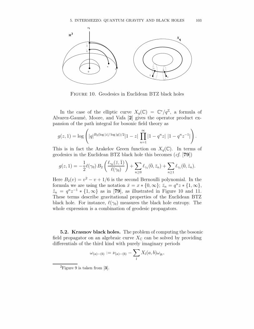
5. INTERMEZZO: QUANTUM GRAVITY AND BLACK HOLES 103
-x
1-
x1
-x
1-
10
oo
x
H3Xq
Figure 10. Geodesics in Euclidean BTZ black holes
In the case of the elliptic curve Xq(C) = C∗/qZ, a formula ofAlvarez-Gaume, Moore, and Vafa [2] gives the operator product ex-pansion of the path integral for bosonic field theory as
g(z, 1) = log
(|q|B2(log |z|/ log |q|)/2|1− z|
∞∏
n=1
|1− qnz| |1− qnz−1|)
.
This is in fact the Arakelov Green function on Xq(C). In terms ofgeodesics in the Euclidean BTZ black hole this becomes (cf. [79])
g(z, 1) = −1
2`(γ0) B2
(`γ0(z, 1)
`(γ0)
)+∑
n≥0
`γ1(0, zn) +∑
n≥1
`γ1(0, zn).
Here B2(v) = v2 − v + 1/6 is the second Bernoulli polynomial. In theformula we are using the notation x = x ∗ 0,∞; zn = qnz ∗ 1,∞,zn = qnz−1 ∗ 1,∞ as in [79], as illustrated in Figure 10 and 11.These terms describe gravitational properties of the Euclidean BTZblack hole. For instance, `(γ0) measures the black hole entropy. Thewhole expression is a combination of geodesic propagators.
5.2. Krasnov black holes. The problem of computing the bosonicfield propagator on an algebraic curve XC can be solved by providingdifferentials of the third kind with purely imaginary periods
ω(a)−(b) := ν(a)−(b) −∑
l
Xl(a, b)ωgl,
2Figure 9 is taken from [3].
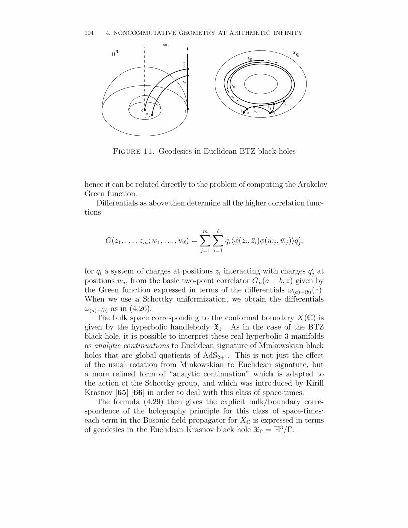
104 4. NONCOMMUTATIVE GEOMETRY AT ARITHMETIC INFINITY
-x-x1-x20-
x1
δ 0
γ0
Xq
qn
x
x-n
0-
oo
10
Η 3
Figure 11. Geodesics in Euclidean BTZ black holes
hence it can be related directly to the problem of computing the ArakelovGreen function.
Differentials as above then determine all the higher correlation func-tions
G(z1, . . . , zm; w1, . . . , w`) =
m∑
j=1
∑
i=1
qi〈φ(zi, zi)φ(wj, wj)〉q′j,
for qi a system of charges at positions zi interacting with charges q′j atpositions wj, from the basic two-point correlator Gµ(a− b, z) given bythe Green function expressed in terms of the differentials ω(a)−(b)(z).When we use a Schottky uniformization, we obtain the differentialsω(a)−(b) as in (4.26).
The bulk space corresponding to the conformal boundary X(C) isgiven by the hyperbolic handlebody XΓ. As in the case of the BTZblack hole, it is possible to interpret these real hyperbolic 3-manifoldsas analytic continuations to Euclidean signature of Minkowskian blackholes that are global quotients of AdS2+1. This is not just the effectof the usual rotation from Minkowskian to Euclidean signature, buta more refined form of “analytic continuation” which is adapted tothe action of the Schottky group, and which was introduced by KirillKrasnov [65] [66] in order to deal with this class of space-times.
The formula (4.29) then gives the explicit bulk/boundary corre-spondence of the holography principle for this class of space-times:each term in the Bosonic field propagator for XC is expressed in termsof geodesics in the Euclidean Krasnov black hole XΓ = H3/Γ.
6. DUAL GRAPH AND NONCOMMUTATIVE GEOMETRY 105
6. Dual graph and noncommutative geometry
Manin’s result on the Arakelov Green function and hyperbolic ge-ometry suggests a geometric model for the dual graph of the mysteriousfiber at arithmetic infinity.
In fact, the result discussed above on the Green function has ananalog, due to Drinfel’d and Manin [56] in the case of a finite primewith a totally split fiber. This is the case where the p-adic completionadmits a Schottky uniformization by a p-adic Schottky group.
6.1. Schottky–Mumford curves. If K is a given finite extensionof Qp, we denote by O ⊂ K its ring of integers, by m ⊂ O the maximalideal, and by k the residue field k = O/m. This is a finite field ofcardinality q = card(O/m).
It is well known that a curve X over a finite extension K of Qp,which is k-split degenerate, for k the residue field, admits a p-adicuniformization by a p-adic Schottky group Γ acting on the Bruhat-Titstree ∆K.
The Bruhat-Tits tree is obtained by considering free O-modules ofrank 2, with the equivalence relation that M1 ∼ M2 iff ∃λ ∈ K∗ suchthat M1 = λM2. The vertices of the tree consist of these equivalenceclasses. A distance is introduced on this set by prescribing that ifM1, M2 ∈ ∆0
K , with M1 ⊃M2, then
M1/M2 ' O/ml ⊕O/mk, l, k ∈ N
and we set the distance to be d(M1, M2) = |l − k|. We form thetree ∆K, by adding an edge between any two pairs of vertices withd(M1, M2) = 1. This gives a connected, locally finite tree withq + 1 edges departing from each vertex. The group PGL(2, K) actstransitively (on the left) by isometries.
The Bruhat-Tits tree ∆K is the analog of the 3-dimensional realhyperbolic space H3 at the infinite primes. The set of ends of ∆K isidentified with P1(K), just as we have P1(C) = ∂H3 in the case atinfinity.
A p-adic Schottky group Γ is a discrete subgroup of PGL(2, K)which consists of hyperbolic elements γ (the eigenvalues of γ in Khave different valuation), and which is isomorphic to a free group ing generators. We still denote by ΛΓ ⊂ P1(K) the limit set, that is,the closure of the set of points in P1(K) that are fixed points of someγ ∈ Γ \ 1. As in the case at infinity, we have card(ΛΓ) < ∞ if andonly if Γ = (γ)Z, for some γ ∈ Γ (the genus one case). We denote by
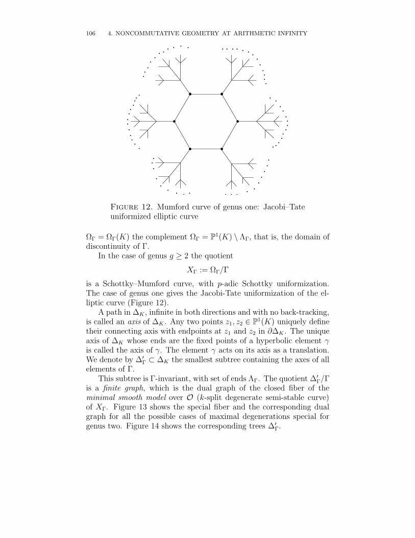
106 4. NONCOMMUTATIVE GEOMETRY AT ARITHMETIC INFINITY
. ......
...........
.
..
..
. . . . . . .
.
.....
. .. .
.........
.
.
.... . . . . . . . . . . . . . .
Figure 12. Mumford curve of genus one: Jacobi–Tateuniformized elliptic curve
ΩΓ = ΩΓ(K) the complement ΩΓ = P1(K) \ ΛΓ, that is, the domain ofdiscontinuity of Γ.
In the case of genus g ≥ 2 the quotient
XΓ := ΩΓ/Γ
is a Schottky–Mumford curve, with p-adic Schottky uniformization.The case of genus one gives the Jacobi-Tate uniformization of the el-liptic curve (Figure 12).
A path in ∆K , infinite in both directions and with no back-tracking,is called an axis of ∆K. Any two points z1, z2 ∈ P1(K) uniquely definetheir connecting axis with endpoints at z1 and z2 in ∂∆K . The uniqueaxis of ∆K whose ends are the fixed points of a hyperbolic element γis called the axis of γ. The element γ acts on its axis as a translation.We denote by ∆′
Γ ⊂ ∆K the smallest subtree containing the axes of allelements of Γ.
This subtree is Γ-invariant, with set of ends ΛΓ. The quotient ∆′Γ/Γ
is a finite graph, which is the dual graph of the closed fiber of theminimal smooth model over O (k-split degenerate semi-stable curve)of XΓ. Figure 13 shows the special fiber and the corresponding dualgraph for all the possible cases of maximal degenerations special forgenus two. Figure 14 shows the corresponding trees ∆′
Γ.
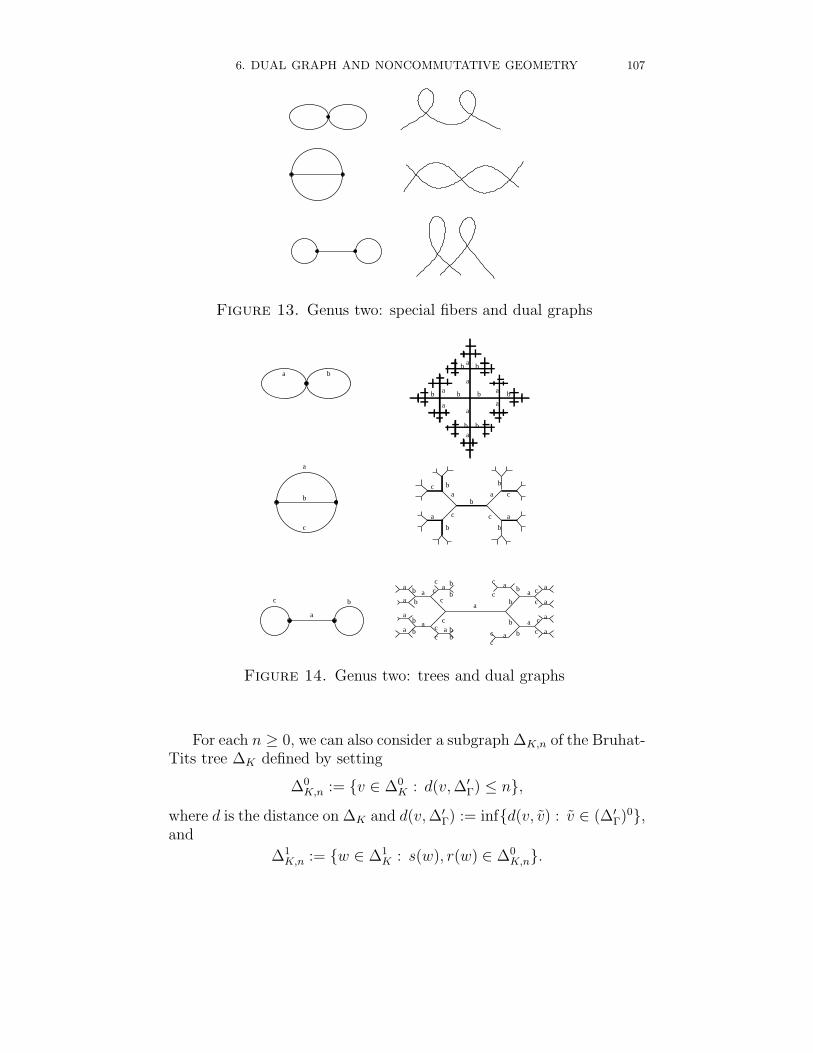
6. DUAL GRAPH AND NONCOMMUTATIVE GEOMETRY 107
Figure 13. Genus two: special fibers and dual graphs
a
bca b
b a
ab
b c
c
c
c
c
ccc
cc
a bb
b
ba
a
ab
b
b
b
a
a
a
a
a
a
a
a
a
acc
c
c
a
b
c
ba
c
a
c
b
c
b
a
b
a
bc
a ba
a
a
a
bb
bb
bb
bb a
a
a
a
Figure 14. Genus two: trees and dual graphs
For each n ≥ 0, we can also consider a subgraph ∆K,n of the Bruhat-Tits tree ∆K defined by setting
∆0K,n := v ∈ ∆0
K : d(v, ∆′Γ) ≤ n,
where d is the distance on ∆K and d(v, ∆′Γ) := infd(v, v) : v ∈ (∆′
Γ)0,and
∆1K,n := w ∈ ∆1
K : s(w), r(w) ∈ ∆0K,n.
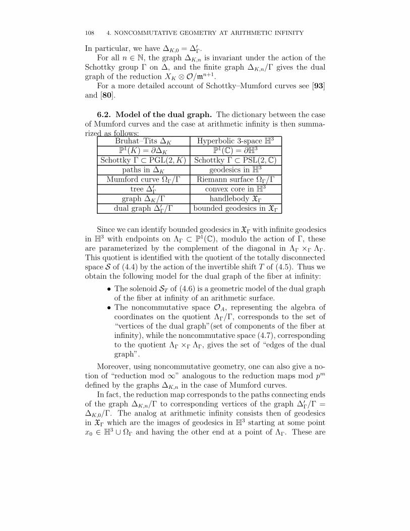
108 4. NONCOMMUTATIVE GEOMETRY AT ARITHMETIC INFINITY
In particular, we have ∆K,0 = ∆′Γ.
For all n ∈ N, the graph ∆K,n is invariant under the action of theSchottky group Γ on ∆, and the finite graph ∆K,n/Γ gives the dualgraph of the reduction XK ⊗O/mn+1.
For a more detailed account of Schottky–Mumford curves see [93]and [80].
6.2. Model of the dual graph. The dictionary between the caseof Mumford curves and the case at arithmetic infinity is then summa-rized as follows:
Bruhat–Tits ∆K Hyperbolic 3-space H3
P1(K) = ∂∆K P1(C) = ∂H3
Schottky Γ ⊂ PGL(2, K) Schottky Γ ⊂ PSL(2, C)paths in ∆K geodesics in H3
Mumford curve ΩΓ/Γ Riemann surface ΩΓ/Γtree ∆′
Γ convex core in H3
graph ∆K/Γ handlebody XΓ
dual graph ∆′Γ/Γ bounded geodesics in XΓ
Since we can identify bounded geodesics in XΓ with infinite geodesicsin H3 with endpoints on ΛΓ ⊂ P1(C), modulo the action of Γ, theseare parameterized by the complement of the diagonal in ΛΓ ×Γ ΛΓ.This quotient is identified with the quotient of the totally disconnectedspace S of (4.4) by the action of the invertible shift T of (4.5). Thus weobtain the following model for the dual graph of the fiber at infinity:
• The solenoid ST of (4.6) is a geometric model of the dual graphof the fiber at infinity of an arithmetic surface.• The noncommutative space OA, representing the algebra of
coordinates on the quotient ΛΓ/Γ, corresponds to the set of“vertices of the dual graph”(set of components of the fiber atinfinity), while the noncommutative space (4.7), correspondingto the quotient ΛΓ ×Γ ΛΓ, gives the set of “edges of the dualgraph”.
Moreover, using noncommutative geometry, one can also give a no-tion of “reduction mod ∞” analogous to the reduction maps mod pm
defined by the graphs ∆K,n in the case of Mumford curves.In fact, the reduction map corresponds to the paths connecting ends
of the graph ∆K,n/Γ to corresponding vertices of the graph ∆′Γ/Γ =
∆K,0/Γ. The analog at arithmetic infinity consists then of geodesicsin XΓ which are the images of geodesics in H3 starting at some pointx0 ∈ H3 ∪ ΩΓ and having the other end at a point of ΛΓ. These are
7. ARITHMETIC VARIETIES AND L–FACTORS 109
parameterized by the set
ΛΓ ×Γ (H3 ∪ ΩΓ).
Thus, in terms of noncommutative geometry, the reduction mod∞corresponds to a compactification of the homotopy quotient
ΛΓ ×Γ H3 = ΛΓ ×Γ EΓ
whereBΓ = H3/Γ = XΓ.
Thus, we can view ΛΓ/Γ as the quotient of a foliation on the ho-motopy quotient with contractible leaves H3. The reduction mod ∞ isthen given by the µ-map
µ : K∗+1(ΛΓ ×Γ H3)→ K∗(C(ΛΓ) o Γ).
This shows that the noncommutative space (OA,H,D) is closely re-lated ot the geometry of the fiber at arithmetic infinity of an algebraicvariety. One can ask then what arithmetic information is capturedby the Dirac operator D of this spectral triples. We’ll see in the nextsection that (as proved in [44]), the Dirac operator gives another impor-tant arithmetic invariant, namely the local L-factor at the archimedeanprime.
7. Arithmetic varieties and L–factors
An important invariant of arithmetic varieties is the L-function.This is written as a product of contributions from the finite primes andthe archimedean primes,
(4.31)∏
℘∈Spec OK
L℘(Hm(X), s).
We do not plan to give a detailed account on the subject, but we referthe interested reader to [103]. Here we only try to convey some basicideas.
The reason why one needs to consider also the contribution of thearchimedean primes can be seen in the case of the “affine line” Spec(Z),where one has the Riemann zeta function, which is written as the Eulerproduct
(4.32) ζ(s) =∏
p
(1− p−s)−1.
However, to have a nice functional equation, one needs to consider theproduct
(4.33) ζ(s) Γ(s/2)π−s/2,
110 4. NONCOMMUTATIVE GEOMETRY AT ARITHMETIC INFINITY
which includes a contribution of the archimedean prime, expressed interms of the Gamma function
(4.34) Γ(s) =
∫ ∞
0
e−tts−1 dt.
An analogy with ordinary geometry suggests to think of the func-tional equation as a sort of “Poincare duality”, which holds for a com-pact manifold, hence the need to “compactify” arithmetic varieties byadding the archimedean primes and the corresponding archimedeanfibers.
When one looks at an arithmetic variety over a finite prime ℘ ∈Spec(OK), the fact that the reduction lives over a residue field of posi-tive characteristic implies that there is a special operator, the geometricFrobenius Fr∗℘, acting on a suitable cohomology theory (etale cohomol-
ogy), induced by the Frobenius automorphism φ℘ of Gal(Fp/Fp).The local L-factors of (4.31) at finite primes encode the action of
the geometric Frobenius in the form [103]
(4.35) L℘(Hm(X), s) = det(1− Fr∗℘N(℘)−s|Hm(X, Q`)
I℘)−1
.
Here we are considering the action of the geometric Frobenius Fr∗℘on the inertia invariants Hm(X, Q`)
I℘ of the etale cohomology. An in-troduction to etale cohomology and a precise definition of these arith-metic structures is beyond the scope of these notes. In fact, our pri-mary concern will only be the contribution of the archimedean primesto (4.31), where the construction will be based on ordinary de Rhamcohomology. Thus, we only give a quick and somewhat heuristic ex-planation of (4.35). We refer to [103] [107] for a detailed and rigorousaccount and for the precise hypotheses under which the following holds.
For X a smooth projective algebraic variety (in any dimension)defined over Q, the notation X denotes
X := X ⊗ Spec(Q),
where Q is an algebraic closure. For ` a prime, the cohomology H∗(X, Q`)is a finite dimensional Q`-vector space satisfying
(4.36) H i(X(C), C) ' H i(X, Q`)⊗ C.
The absolute Galois group Gal(Q/Q) acts on H∗(X, Q`).Similarly, we can consider H∗(X, Q`) for X defined over a number
field K. For ℘ ∈ Spec(OK) and ` a prime such that (`, q) = 1, where qis the cardinality of the residue field at ℘, the inertia invariants
(4.37) H∗(X, Q`)I℘ ⊂ H∗(X, Q`)
7. ARITHMETIC VARIETIES AND L–FACTORS 111
are the part of the `-adic cohomology where the inertia group at ℘ actstrivially. The latter is defined as
(4.38) I℘ = Ker(D℘ → Gal(Fp/Fp)),
with D℘ = σ ∈ Gal(Q/Q) | σ(℘) = ℘. The Frobenius automorphismof Gal(Fp/Fp) lifts to φ℘ ∈ D℘/I℘ and induces the geometric Frobe-nius F ∗
℘ := (φ−1℘ )∗ acting on H∗(X, Q`)
I℘. We use the notation N in(4.35) for the norm map. Thus, we can write the local L-factor (4.35)equivalently as
(4.39) L℘(Hm(X), s) =∏
λ∈Spec(Fr∗℘)
(1− λq−s)− dimHm(XΓ)I℘λ ,
where Hm(XΓ)I℘
λ is the eigenspace of the Frobenius with eigenvalue λ.For our purposes, what is most important to retain from the dis-
cussion above is that the local L-factor (4.35) depends upon the data
(4.40)(H∗(X, Q`)
I℘, F r∗℘)
of a vector space, which has a cohomological interpretation, togetherwith a linear operator.
7.1. Archimedean L-factors. Since etale cohomology satisfiesthe compatibility (4.36), if we again resort to the general philosophy, ac-cording to which we can work with the smooth complex manifold X(C)and gain information on the “closed fiber” at arithmetic infinity, we areled to expect that the contribution of the archimedean primes to theL-function may be expressed in terms of the cohomology H∗(X(C), C),or equivalently in terms of de Rham cohomology.
In fact, Serre showed ([103]) that the expected contribution of thearchimedean primes depends upon the Hodge structure
(4.41) Hm(X(C)) = ⊕p+q=mHp,q(X(C))
and is again expressed in terms of Gamma functions, as in the case of(4.33). Namely, one has a product of Gamma functions according tothe Hodge numbers hp,q,(4.42)
L(H∗, s) =
∏p,q ΓC(s−min(p, q))hp,q
∏p<q ΓC(s− p)hp,q ∏
p ΓR(s− p)hp,+ΓR(s− p + 1)hp,−
where the two cases correspond, respectively, to the complex and thereal embeddings. Here hp,± is the dimension of the ±(−1)p-eigenspaceof the involution on Hp,p induced by the real structure and
(4.43) ΓC(s) := (2π)−sΓ(s), ΓR(s) := 2−1/2π−s/2Γ(s/2).
112 4. NONCOMMUTATIVE GEOMETRY AT ARITHMETIC INFINITY
One of the general ideas in arithmetic geometry is that one shouldalways seek a unified picture of what happens at the finite and at theinfinite primes. In particular, there should be a suitable reformula-tion of the local factors (4.35) and (4.42) where both formulae can beexpressed in the same way.
Seeking a unified description of local L-factors at finite and infiniteprimes, Deninger in [52], [53], [54] expressed both (4.35) and (4.42) asinfinite determinants.
Recall that the Ray-Singer determinant of an operator T with purepoint spectrum with finite multiplicities mλλ∈Spec(T ) is defined as
(4.44) det∞
(s− T ) := exp
(− d
dzζT (s, z)|z=0
)
where the zeta function of T is defined as
(4.45) ζT (s, z) =∑
λ∈Spec(T )
mλ(s− λ)−z.
Suitable conditions for the convergence of these expressions in the caseof the local factors are described in [78].
Deninger showed that (4.39) can be written equivalently in the form
(4.46) L℘(Hm(X), s)−1 = det∞
(s−Θq),
for an operator with spectrum(4.47)
Spec(s−Θq) =
2πi
log q
(log q
2πi(s− αλ) + n
): n ∈ Z, λ ∈ Spec(Fr∗v)
,
with multiplicities dλ and with qαλ = λ.Moreover, the local factor (4.42) at infinity can be written similarly
in the form
(4.48) L(Hq(X), s) = det∞
(1
2π(s− Φ)|Hm
)−1
where Hm is an infinite dimensional vector space and Φ is a linear oper-ator with spectrum Spec(Φ) = Z and finite multiplicites. This operatoris regarded as a “logarithm of Frobenius” at arithmetic infinity.
Given Deninger’s formulae (4.46) and (4.48), it is natural to ask fora cohomological interpretation of the data
(4.49) (Hm, Φ)
somewhat analogous to (4.40).
7. ARITHMETIC VARIETIES AND L–FACTORS 113
7.2. Arithmetic surfaces: L-factor and Dirac operator. Letus now return to the special case of arithmetic surfaces, in the case ofgenus g ≥ 2.
At an archimedean prime, we consider the Riemann surface Xα(C)with a Schottky uniformization
X(C) = ΩΓ/Γ.
In the case of a real embedding we can assume that the choice of Schot-tky uniformization is the one that corresponds to the real structure,obtained by cutting X(C) along the real locus X(R).
Consider the spectral triple (OA,H,D) associated to the Schottkygroup Γ acting on its limit set ΛΓ. Since the spectral triple is notfinitely summable, we do not have zeta functions of the spectral triplein the form Tr(a|D|z). However, we can consider the restriction of Dto a suitable subspace of H, where it becomes of trace class.
In particular, consider the zeta function
(4.50) ζπV ,D(s, z) :=∑
λ∈Spec(D)
Tr (πVΠ(λ,D)) (s− λ)−z
where πV is the orthogonal projection of H onto the subspace V of0⊕ L ⊂ H defined by
(4.51) Πn πV Πn =
g∑
i=1
Sni S∗
in,
on L, where Πn are the spectral projections of the Dirac operator,Πn = Π(−n,D), for n ≥ 0.
In the case of an arithmetic surface the interesting local factor is theone for the first cohomology, L(H1(X), s). This can be computed ([44],[46]) from the zeta function (4.50) of the spectral triple (OA,H,D).
Theorem 7.1. The local L-factor (4.42) is given by
(4.52) L(H1(X), s) = exp
(− d
dzζπV , D
2π
( s
2π, z)|z=0
)−1
.
In the case of a real embedding, the same holds, with the projectionπV ,F∞=id onto the +1 eigenspace of the involution F∞ induced by thereal structure on V.
This result shows in particular that, for the special case of arith-metic surfaces with X(C) of genus g ≥ 2, the pair
(4.53) (V ⊂ L,D|V)
114 4. NONCOMMUTATIVE GEOMETRY AT ARITHMETIC INFINITY
is a possible geometric construction of the pair (H1, Φ) of (4.49). Inparticular, the Dirac operator of the spectral triple has an arithmeticmeaning, in as it recovers the “logarithm of Frobenius”
(4.54) D|V = Φ.
If we look more closely at the subspace V of the Hilbert space H,we see that it has a simple geometric interpretation in terms of thegeodesics in the handlebody XΓ. Recall that the filtered subspace Pof L = L2(ΛΓ, dµ) describes 1-cochains on the mapping torus ST , withP/δP = H1(ST ).
The mapping torus ST is a copy of the tangle of bounded geodesicsinside XΓ. Among these geodesics there are g “fundamental” closedgeodesics that correspond to the generators of Γ (they correspond togeodesics in H3 connecting the fixed points z±(γi), for i = 1, . . . , g).Topologically, these are the g core handles of the handlebody XΓ andthey generate the homology H1(XΓ).
Consider the cohomology H1(ST ). Suppose that we wish to findelements of H1(ST ) supported on these fundamental closed geodesics.This is impossible, because forms on ST are defined by functions inC(S, Z), that are supported on some clopen set covering the totallydisconnected set S, which contains no isolated points. However, it ispossible to choose a sequence of 1-cochains on ST whose supports aresmaller and smaller clopen sets containing the infinite word in S corre-sponding to one of the g fundamental geodesics. The finite dimensionalsubspace Vn = V ∩ Pn
Vn ⊂ Pn dimVn = 2g
gives representatives of exactly such cohomology classes in H 1(ST ).(We get 2g instead of g because we take into account the two possiblechoices of orientation.)
Thus, this gives us, in the case of arithmetic surfaces, a cohomologi-cal interpretation of the space H1 = V in the pair (4.49). Moreover, theSchottky uniformization also provides us with a way of expressing thiscohomology H1 = V in terms of the de Rham cohomology H1(X(C)).In fact, we have already seen in the calculation of the Green functionthat, under the hypothesis that dimH(ΛΓ) < 1, to each generator γi ofthe Schottky group we can associate a holomorphic differential on theRiemann surface X(C) by (4.24). The map
γi 7→ ωγi=
∑
h∈C(|γi)
d log〈hz+(γi), hz−(γi), z, z0〉
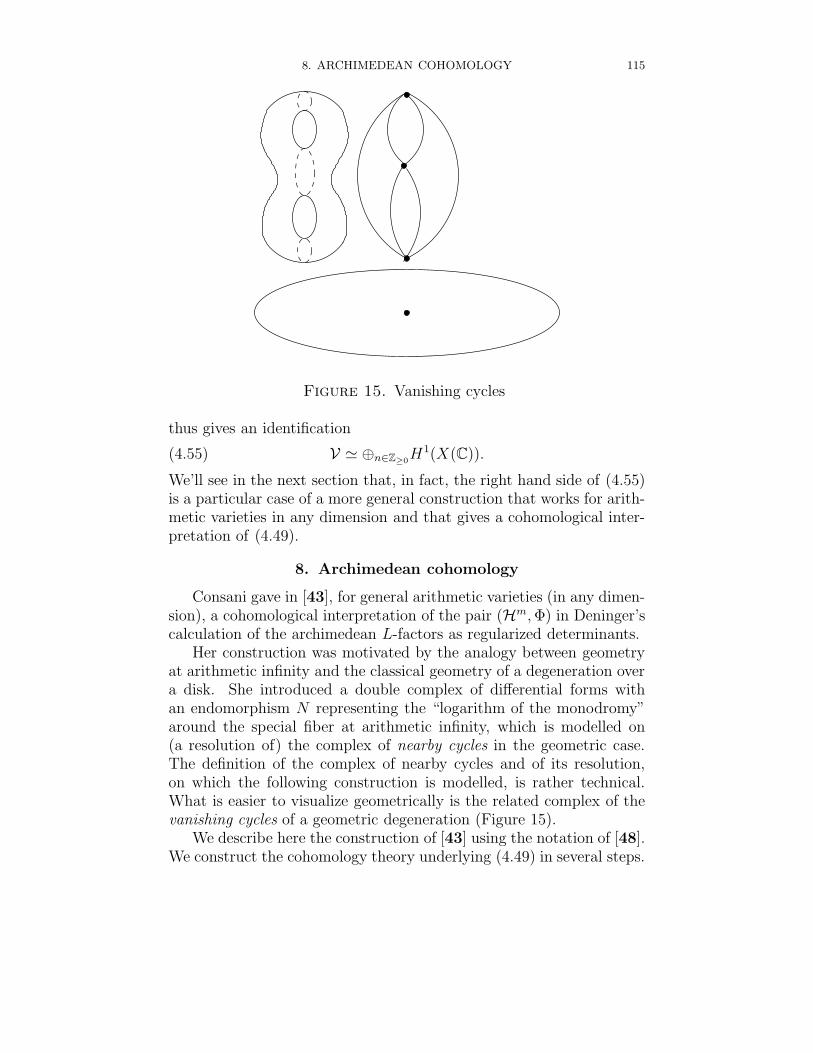
8. ARCHIMEDEAN COHOMOLOGY 115
Figure 15. Vanishing cycles
thus gives an identification
(4.55) V ' ⊕n∈Z≥0H1(X(C)).
We’ll see in the next section that, in fact, the right hand side of (4.55)is a particular case of a more general construction that works for arith-metic varieties in any dimension and that gives a cohomological inter-pretation of (4.49).
8. Archimedean cohomology
Consani gave in [43], for general arithmetic varieties (in any dimen-sion), a cohomological interpretation of the pair (Hm, Φ) in Deninger’scalculation of the archimedean L-factors as regularized determinants.
Her construction was motivated by the analogy between geometryat arithmetic infinity and the classical geometry of a degeneration overa disk. She introduced a double complex of differential forms withan endomorphism N representing the “logarithm of the monodromy”around the special fiber at arithmetic infinity, which is modelled on(a resolution of) the complex of nearby cycles in the geometric case.The definition of the complex of nearby cycles and of its resolution,on which the following construction is modelled, is rather technical.What is easier to visualize geometrically is the related complex of thevanishing cycles of a geometric degeneration (Figure 15).
We describe here the construction of [43] using the notation of [48].We construct the cohomology theory underlying (4.49) in several steps.
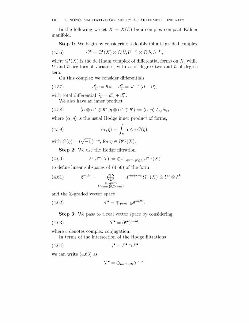
116 4. NONCOMMUTATIVE GEOMETRY AT ARITHMETIC INFINITY
In the following we let X = X(C) be a complex compact Kahlermanifold.
Step 1: We begin by considering a doubly infinite graded complex
(4.56) C• = Ω•(X)⊗ C[U, U−1]⊗ C[~, ~−1],
where Ω•(X) is the de Rham complex of differential forms on X, whileU and ~ are formal variables, with U of degree two and ~ of degreezero.
On this complex we consider differentials
(4.57) d′C := ~ d, d′′
C =√−1(∂ − ∂),
with total differential δC = d′C + d′′
C .We also have an inner product
(4.58) 〈α⊗ U r ⊗ ~k, η ⊗ U s ⊗ ~t〉 := 〈α, η〉 δr,sδk,t
where 〈α, η〉 is the usual Hodge inner product of forms,
(4.59) 〈α, η〉 =∫
X
α ∧ ∗C(η),
with C(η) = (√−1 )p−q, for η ∈ Ωp,q(X).
Step 2: We use the Hodge filtration
(4.60) F pΩm(X) := ⊕p′+q=m, p′≥p Ωp′,q(X)
to define linear subspaces of (4.56) of the form
(4.61) Cm,2r =⊕
p+q=mk≥max0,2r+m
F m+r−k Ωm(X) ⊗ U r ⊗ ~k
and the Z-graded vector space
(4.62) C• = ⊕•=m+2rCm,2r.
Step 3: We pass to a real vector space by considering
(4.63) T • = (C•)c=id,
where c denotes complex conjugation.In terms of the intersection of the Hodge filtrations
(4.64) γ• = F • ∩ F •
we can write (4.63) as
T • = ⊕•=m+2rT m,2r
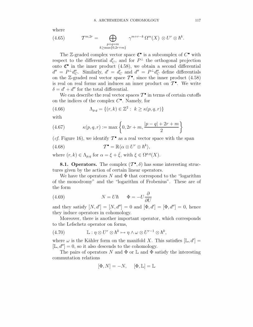
8. ARCHIMEDEAN COHOMOLOGY 117
where
(4.65) T m,2r =⊕
p+q=mk≥max0,2r+m
γm+r−k Ωm(X) ⊗ U r ⊗ ~k.
The Z-graded complex vector space C• is a subcomplex of C• withrespect to the differential d′
C , and for P⊥ the orthogonal projectiononto C• in the inner product (4.58), we obtain a second differentiald′′ = P⊥d′′
C . Similarly, d′ = d′C and d′′ = P⊥d′′
C define differentialson the Z-graded real vector space T •, since the inner product (4.58)is real on real forms and induces an inner product on T •. We writeδ = d′ + d′′ for the total differential.
We can describe the real vector spaces T • in terms of certain cutoffson the indices of the complex C•. Namely, for
(4.66) Λp,q = (r, k) ∈ Z2 : k ≥ κ(p, q, r)with
(4.67) κ(p, q, r) := max
0, 2r + m,
|p− q|+ 2r + m
2
(cf. Figure 16), we identify T • as a real vector space with the span
(4.68) T • = R〈α⊗ U r ⊗ ~k〉,where (r, k) ∈ Λp,q for α = ξ + ξ, with ξ ∈ Ωp,q(X).
8.1. Operators. The complex (T •, δ) has some interesting struc-tures given by the action of certain linear operators.
We have the operators N and Φ that correspond to the “logarithmof the monodromy” and the “logarithm of Frobenius”. These are ofthe form
(4.69) N = U~ Φ = −U∂
∂U
and they satisfy [N, d′] = [N, d′′] = 0 and [Φ, d′] = [Φ, d′′] = 0, hencethey induce operators in cohomology.
Moreover, there is another important operator, which correspondsto the Lefschetz operator on forms,
(4.70) L : η ⊗ U r ⊗ ~k 7→ η ∧ ω ⊗ U r−1 ⊗ ~k,
where ω is the Kahler form on the manifold X. This satisfies [L, d′] =[L, d′′] = 0, so it also descends to the cohomology.
The pairs of operators N and Φ or L and Φ satisfy the interestingcommutation relations
[Φ, N ] = −N, [Φ, L] = L
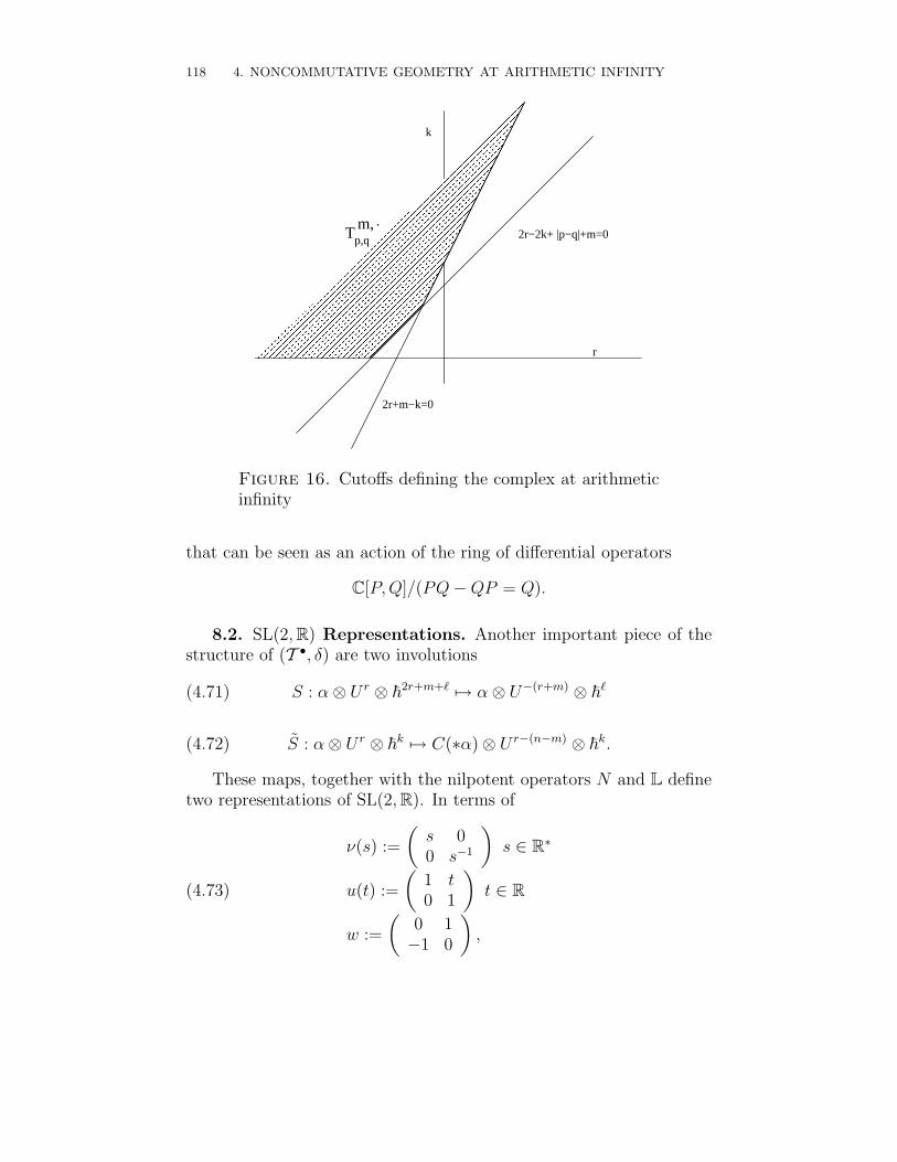
118 4. NONCOMMUTATIVE GEOMETRY AT ARITHMETIC INFINITY
r
.m,p,q 2r−2k+ |p−q|+m=0
2r+m−k=0
k
T
Figure 16. Cutoffs defining the complex at arithmeticinfinity
that can be seen as an action of the ring of differential operators
C[P, Q]/(PQ−QP = Q).
8.2. SL(2, R) Representations. Another important piece of thestructure of (T •, δ) are two involutions
(4.71) S : α⊗ U r ⊗ ~2r+m+` 7→ α⊗ U−(r+m) ⊗ ~`
(4.72) S : α⊗ U r ⊗ ~k 7→ C(∗α)⊗ U r−(n−m) ⊗ ~k.
These maps, together with the nilpotent operators N and L definetwo representations of SL(2, R). In terms of
(4.73)
ν(s) :=
(s 00 s−1
)s ∈ R∗
u(t) :=
(1 t0 1
)t ∈ R
w :=
(0 1−1 0
),
8. ARCHIMEDEAN COHOMOLOGY 119
the representations σL and σR are given by
(4.74)
σL(ν(s)) = s−n+m σR(ν(s)) = s2r+m
σL(u(t)) = exp(t L) σR(u(t)) = exp(t N)
σL(w) = (√−1)n C S σR(w) = C S.
Of these representations, σL extends to an action by bounded op-erators on the Hilbert completion of T • in the inner product (4.58),while the action of the subgroup ν(s), s ∈ R∗ of SL(2, R) via the rep-resentation σR on this Hilbert space is by unbounded densely definedoperators.
8.3. Renormalization group and monodromy. This very gen-eral structure, which exists for varieties in any dimension, also has in-teresting connections to noncommutative geometry. For instance, wecan see that in fact the map N does play the role of the “logarithmof the monodromy” using an analog in our context of the theory ofrenormalization a la Connes–Kreimer [31].
In the classical case of a geometric degeneration on a disk, themonodromy around the special fiber is defined as the map
(4.75) T = exp(−2π√−1 Res0(∇))
where
(4.76) N = Res0(∇)
is the residue at zero of the connection, acting as an endomorphism ofthe cohomology.
In our setting, we consider loops φµ with values in the group G =Aut(T •
C , δ), depending on a “mass parameter” µ ∈ C∗. Here T •C is the
complexification of the real vector space T •. The Birkhoff decomposi-tion of a loop φµ consists in the multiplicative decomposition
(4.77) φµ(z) = φ−µ (z)−1 φ+
µ (z),
for z ∈ ∂∆ ⊂ P1(C), where ∆ is a small disk centered at zero. Of thetwo terms in the right hand side of (4.77), φ+
µ extends to a holomorphic
function on ∆ and φ−µ to a holomorphic functions on P1(C) r ∆ with
values in G. We normalize (4.77) by requiring that φ−µ (∞) = 1.
By analogy with the Connes–Kreimer theory of renormalization werequire the following properties of (4.77):
• The time evolution
(4.78) θt : a 7→ e−tΦa etΦ
120 4. NONCOMMUTATIVE GEOMETRY AT ARITHMETIC INFINITY
acts by scaling
(4.79) φλµ(ε) = θtε φµ(ε),
for λ = et ∈ R∗+ and ε ∈ ∂∆.
• The term φ−µ = φ− in the Birkhoff decomposition is indepen-
dent of the energy scale µ.
The residue of a loop φµ, as in [31], is given by
(4.80) Res φ =d
dz
(φ−(1/z)−1
)|z=0
and the beta function of renormalization is
(4.81) β = Υ Res φ, with Υ =d
dtθt|t=0.
In our setting, there is a natural choice of the time evolution, givenby the “geodesic flow” associated to the “Dirac operator” Φ, namely
(4.82) θt(a) = e−tΦ a etΦ.
This gives
(4.83) Υ(a) =d
dtθt(a)|t=0 = [a, Φ].
There is a scattering formula ([31]), by which one can reconstructφ− from the residue. Namely, we can write
φ−(z)−1 = 1 +∑
k≥1
dk z−k,
with
(4.84) dk =
∫
s1≥···≥sk≥0
θ−s1(β) · · · θ−sk(β) ds1 · · ·dsk.
The renormalization group is given by
(4.85) ρ(λ) = limε→0
φ−(ε) θtε(φ−(ε)−1),
for λ = et ∈ R∗+.
Thus, we only need to specify the residue in order to have the cor-responding renormalization theory associated to (T •
C , δ). By analogywith the case of the geometric degeneration (4.76) it is natural to re-quire that Res φ = N . We then have ([48]):
Proposition 8.1. A loop φµ in G = Aut(T •C , δ) with Res φµ = N ,
subject to (4.79) and with φ− independent of µ, satisfies
φµ(z) = exp
(µz
zN
)
8. ARCHIMEDEAN COHOMOLOGY 121
with Birkhoff decomposition
φµ(z) = exp(−N/z) exp
(µz − 1
zN
).
In fact, by (4.83) and Res φµ = N we have β = [N, Φ] = N andθt(N) = et N , hence the scattering formula (4.84) gives
φ−(z) = exp(−N/z)
and the scaling property (4.79) determines
φµ(z) = exp
(µz
zN
).
The part of the Birkhoff decomposition that is regular at z = 0satisfies φ+
µ (0) = µN .The renormalization group is of the form
(4.86) ρ(λ) = λN = exp(tN),
which, through the representation σR of SL(2, R), corresponds to thehorocycle flow on SL(2, R)
ρ(λ) = u(t) =
(1 t0 1
).
The Birkhoff decomposition (4.77) gives a trivialization of a princi-pal G-bundle over P1(C). We can consider the associated vector bundleE•µ with fiber T •
C .Moreover, we obtain a Fuchsian connection ∇µ on this bundle,
(4.87) ∇µ : E•µ → E•µ ⊗O∆Ω•
∆(log 0),
where the notation Ω•∆(log 0) denotes forms with logarithmic poles at
0. This has the form
∇µ = N
(1
z+
d
dz
µz − 1
z
)dz,
with local gauge potentials
−φ+(z)−1 log π(γ) dz
zφ+(z) + φ+(z)−1 dφ+(z)
with respect to the monodromy representation
π : π1(∆∗) = Z→ G
given by
(4.88) π(γ) = exp(−2π√−1 N)
122 4. NONCOMMUTATIVE GEOMETRY AT ARITHMETIC INFINITY
for γ the generator of π1(∆∗). This corresponds to (4.75) in the classical
geometric case. This Fuchsian connection has residue
Resz=0∇µ = N
as in the geometric case (4.76).
8.4. Local factor and archimedean cohomology. In [43] Con-sani showed that the data (Hm, Φ) of (4.49) can be identified with
(H•(T •, δ)N=0, Φ
),
where H•(T •, δ) is the hypercohomology (the cohomology with respectto the total differential δ) of the complex T • and H•(T •, δ)N=0 is thekernel of the map induced by N on cohomology. The operator Φ isthe one induced on cohomology by that of (4.69). She called Hm 'H•(T •, δ)N=0 the archimedean cohomology.
This can also be viewed (cf. [43]) as a piece of the cohomology ofthe cone of the monodromy N . This is the complex
(4.89) Cone(N)• = T • ⊕ T •[+1]
with differential
D =
(δ −N0 δ
).
The complex (4.89) inherits a positive definite inner product fromT •, which descends on cohomology. The representation σL of SL(2, R)on T • induces a representation on Cone(N)•. The corresponding rep-resentation dσL : g→ End(T •) of the Lie algebra g = sl(2, R) extendsto a representation of the universal enveloping algebra U(g) on T • andon Cone(N)•. This gives a representation in the algebra of boundedoperators on the Hilbert completion of Cone(N)• in the inner product.
Theorem 8.2. The triple
(A,H,D) = (U(g), H•(Cone(N)), Φ)
has the properties that D = D∗ and that (1 + D2)−1/2 is a compactoperator. The commutators [D, a] are bounded operators for all a ∈U(g) and the triple is 1+-summable.
Thus, (A,H,D) has most of the properties of a spectral triple,confirming the fact that the logarithm of Frobenius Φ should be thoughtof as a Dirac operator.
In any case, the structure is sufficient to consider zeta functionsfor this “spectral triple”. In particular, we can recover the alternatingproducts of the local L-factors at infinity from a zeta function of thespectral triple.
8. ARCHIMEDEAN COHOMOLOGY 123
Theorem 8.3. Consider the zeta function
ζa,Φ(z) = Tr(a|Φ|−z)
with a = σL(w). This gives
det∞ σL(w),Φ
(s) =2n∏
m=0
L(Hm(X), s)(−1)m
.
8.5. Arithmetic surfaces: homology and cohomology. Inthe particular case of arithmetic surfaces, there is an identification([43], [44])
(4.90) H•(Cone(N)) ' H• ⊕ H•,
where H• is the archimedean cohomology and H• is its dual under theinvolution S of (4.71).
We can then extend the identification
U : H1 '→ V ⊂ L
of (4.55), by considering a subspace W of the homology H1(ST ) withW ' H•. The homology H1(ST ) can also be computed as a direct limit
H1(ST , Z) = lim−→N
KN ,
where the KN are free abelian of rank (2g − 1)N + 1 for N even and(2g − 1)N + (2g − 1) for N odd. The Z-module KN is generated bythe closed geodesics represented by periodic sequences in S of periodN + 1. These need not be primitive closed geodesics. In terms ofprimitive closed geodesics we can write equivalently
H1(ST , Z) = ⊕∞N=0RN
where the RN are free abelian groups with
rkRN =1
N
∑
d|N
µ(d)rkKN/d,
with µ(d) the Mobius function satisfying∑
d|N µ(d) = δN,1.The pairing of homology and cohomology is given by
〈·, ·〉 : Fn × KN → Z 〈[f ], x〉 = N · f(x).
124 4. NONCOMMUTATIVE GEOMETRY AT ARITHMETIC INFINITY
This determines a graded subspace W ⊂ H1(ST , Z) dual to V ⊂H1(ST ). With the identification
H1 U //
S
V ⊂ H1(ST )
〈 , 〉
H1U //W ⊂ H1(ST ),
we can identify the Dirac operator of (4.16) with the logarithm ofFrobenius
(4.91) D|V⊕V = ΦH1⊕H1 .
CHAPTER 5
Vistas
This last brief chapter is meant to answer the question “where do wego from here?”, namely, to outline just a few among the many possibledirections in which the field is evolving. Some of the topics listedbelow are recent results, some are more speculative thoughts. It alljust serves the purpose of conveying the sense of a certain momentumacquired by this set of topics. More detailed information on recentresults in “arithmetic noncommutative geometry” will be found in thevolume [49] and in the monograph in preparation [37].
Noncommutative geometry of Shimura varieties. The re-sults of [9], [32] and [38] can be seen as arising from a noncommutativeversion of the Shimura varieties Sh(GL1,±1) and Sh(GL2, H
±). Theresults of [83] on the noncommutative boundary of the modular curvesand the modular Hecke algebras of [41] [42] also contribute to illustratethe rich noncommutative geometry associated to the modular tower,i.e. to the Shimura variety Sh(GL2, H
±).It is then a natural idea to seek for a larger class of quantum sta-
tistical mechanical systems associated to more general Shimura va-rieties, and investigate the arithmetic properties of low temperatureKMS states. Shimura varieties have the typical property that theyhave adelic groups of symmetries, so that the problem of compatibilitybetween adelic symmetries and the Galois action on the values of zerotemperature KMS states on an arithmetic subalgebra can be formu-lated very naturally in this context.
A program aimed at constructing analogs of the Bost–Connes sys-tem and of the GL2 system of [32] for a large class of Shimura varietiesis being pursued by Eugene Ha and Frederic Paugam. In their con-struction, one considers a more general Shimura datum (G, X). Theanalog of passing from GL2(Af) to M2(Af) in the GL2 system, or fromA∗
f to Af in the Bost–Connes case, is here achieved by considering asuitable enveloping semigroup M . To the resulting datum (G, X, M)they associate a groupoid (in the category of stacks) whose convolutionalgebra generalizes the algebra A2 of the GL2-system. Their algebracomes with variants depending on the choice of a level structure (which
125
126 5. VISTAS
can be used to avoid the stacky singularities in the groupoid). Thereis a natural time evolution on the resulting algebra, which is defined interms of the data of the level structure, and the resulting system has arich adelic group of symmetries. In particular these results can be seenvery explicitly in the Hilbert modular case. They also obtain throughthis general method quantum statistical mechanical systems naturallyassociated to number fields. Their construction agrees with that of [38]for imaginary quadratic fields. The ongoing investigation of the arith-metic properties of KMS states for these systems will certainly yieldinteresting new results.
Classical Shimura varieties also admit noncommutative boundaries,in the same sense in which a noncommutative boundary of modularcurves was constructed in [83]. F. Paugam studied such noncommuta-tive boundaries [96] [97], described by (the convolution algebras asso-ciated to) double cosets spaces L\G(R)/P (K) where G is a connectedreductive algebraic group over Q, L is an arithmetic subgroup of G(Q),and P (K) is a real parabolic subgroup in G(R). As moduli spaces theydescribe degenerations of complex structures on tori in multifoliations.Paugam’s point of view proceeds largely form Hodge theoretic consid-erations.
A question, in this general perspective, that seems very interestingis whether one can establish a connection between this type of resultson the noncommutative geometry of modular curves and Darmon’sgeneralization of the theory of Heegner points [27].
Spectral triples and arithmetic geometry. Besides the occur-rence of spectral triples in the context of the archimedean factors atarithmetic infinity, discussed in the last part of this book, it would beinteresting to seek other occurrences in number theoretic context.
For example, there may be natural spectral triples associated to thealgebras of the quantum statistical mechanical systems for noncommu-tative Shimura varieties mentioned above.
In the case of the Bost–Connes system, this should be interestinglyrelated to the noncommutative space of Connes’ spectral realization ofthe zeros of the Riemann zeta function, and for the GL2-system to themodular Hecke algebras of Connes–Moscovici hence to modular forms.The cases of more general Shimura varieties mentioned above shouldalso be interesting to consider in this perspective.
Another class of spaces of arithmetic significance that may carryinteresting spectral triples are spaces that, like the Mumford curves(cf. [47]), admit p-adic uniformizations (for instance in the case of theCherednik–Drinfeld theory of p-adic uniformization of Shimura curves),
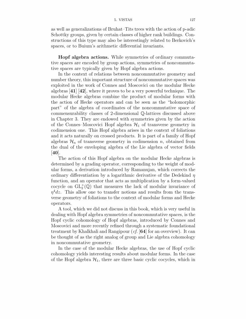
5. VISTAS 127
as well as generalizations of Bruhat–Tits trees with the action of p-adicSchottky groups, given by certain classes of higher rank buildings. Con-structions of this type may also be interestingly related to Berkovich’sspaces, or to Buium’s arithmetic differential invariants.
Hopf algebra actions. While symmetries of ordinary commuta-tive spaces are encoded by group actions, symmetries of noncommuta-tive spaces are typically given by Hopf algebra actions.
In the context of relations between noncommutative geometry andnumber theory, this important structure of noncommutative spaces wasexploited in the work of Connes and Moscovici on the modular Heckealgebras [41] [42], where it proves to be a very powerful technique. Themodular Hecke algebras combine the product of modular forms withthe action of Hecke operators and can be seen as the “holomorphicpart” of the algebra of coordinates of the noncommutative space ofcommensurability classes of 2-dimensional Q-lattices discussed abovein Chapter 3. They are endowed with symmetries given by the actionof the Connes–Moscovici Hopf algebra H1 of transverse geometry incodimension one. This Hopf algebra arises in the context of foliationsand it acts naturally on crossed products. It is part of a family of Hopfalgebras Hn of transverse geometry in codimension n, obtained fromthe dual of the enveloping algebra of the Lie algebra of vector fields[40].
The action of this Hopf algebra on the modular Hecke algebras isdetermined by a grading operator, corresponding to the weight of mod-ular forms, a derivation introduced by Ramanujan, which corrects theordinary differentiation by a logarithmic derivative of the Dedekind ηfunction, and an operator that acts as multiplication by a form-valuedcocycle on GL+
2 (Q) that measures the lack of modular invariance ofη4dz. This allow one to transfer notions and results from the trans-verse geometry of foliations to the context of modular forms and Heckeoperators.
A tool, which we did not discuss in this book, which is very useful indealing with Hopf algebra symmetries of noncommutative spaces, is theHopf cyclic cohomology of Hopf algebras, introduced by Connes andMoscovici and more recently refined through a systematic foundationaltreatment by Khalkhali and Rangipour (cf. [64] for an overview). It canbe thought of as the right analog of group and Lie algebra cohomologyin noncommutative geometry.
In the case of the modular Hecke algebras, the use of Hopf cycliccohomology yields interesting results about modular forms. In the caseof the Hopf algebra H1, there are three basic cyclic cocycles, which in
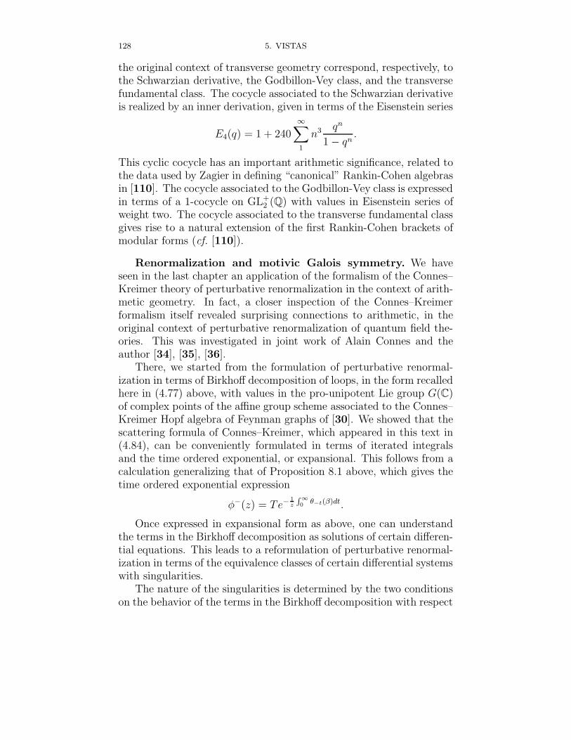
128 5. VISTAS
the original context of transverse geometry correspond, respectively, tothe Schwarzian derivative, the Godbillon-Vey class, and the transversefundamental class. The cocycle associated to the Schwarzian derivativeis realized by an inner derivation, given in terms of the Eisenstein series
E4(q) = 1 + 240∞∑
1
n3 qn
1− qn.
This cyclic cocycle has an important arithmetic significance, related tothe data used by Zagier in defining “canonical” Rankin-Cohen algebrasin [110]. The cocycle associated to the Godbillon-Vey class is expressedin terms of a 1-cocycle on GL+
2 (Q) with values in Eisenstein series ofweight two. The cocycle associated to the transverse fundamental classgives rise to a natural extension of the first Rankin-Cohen brackets ofmodular forms (cf. [110]).
Renormalization and motivic Galois symmetry. We haveseen in the last chapter an application of the formalism of the Connes–Kreimer theory of perturbative renormalization in the context of arith-metic geometry. In fact, a closer inspection of the Connes–Kreimerformalism itself revealed surprising connections to arithmetic, in theoriginal context of perturbative renormalization of quantum field the-ories. This was investigated in joint work of Alain Connes and theauthor [34], [35], [36].
There, we started from the formulation of perturbative renormal-ization in terms of Birkhoff decomposition of loops, in the form recalledhere in (4.77) above, with values in the pro-unipotent Lie group G(C)of complex points of the affine group scheme associated to the Connes–Kreimer Hopf algebra of Feynman graphs of [30]. We showed that thescattering formula of Connes–Kreimer, which appeared in this text in(4.84), can be conveniently formulated in terms of iterated integralsand the time ordered exponential, or expansional. This follows from acalculation generalizing that of Proposition 8.1 above, which gives thetime ordered exponential expression
φ−(z) = Te−1z
R ∞
0θ−t(β)dt.
Once expressed in expansional form as above, one can understandthe terms in the Birkhoff decomposition as solutions of certain differen-tial equations. This leads to a reformulation of perturbative renormal-ization in terms of the equivalence classes of certain differential systemswith singularities.
The nature of the singularities is determined by the two conditionson the behavior of the terms in the Birkhoff decomposition with respect
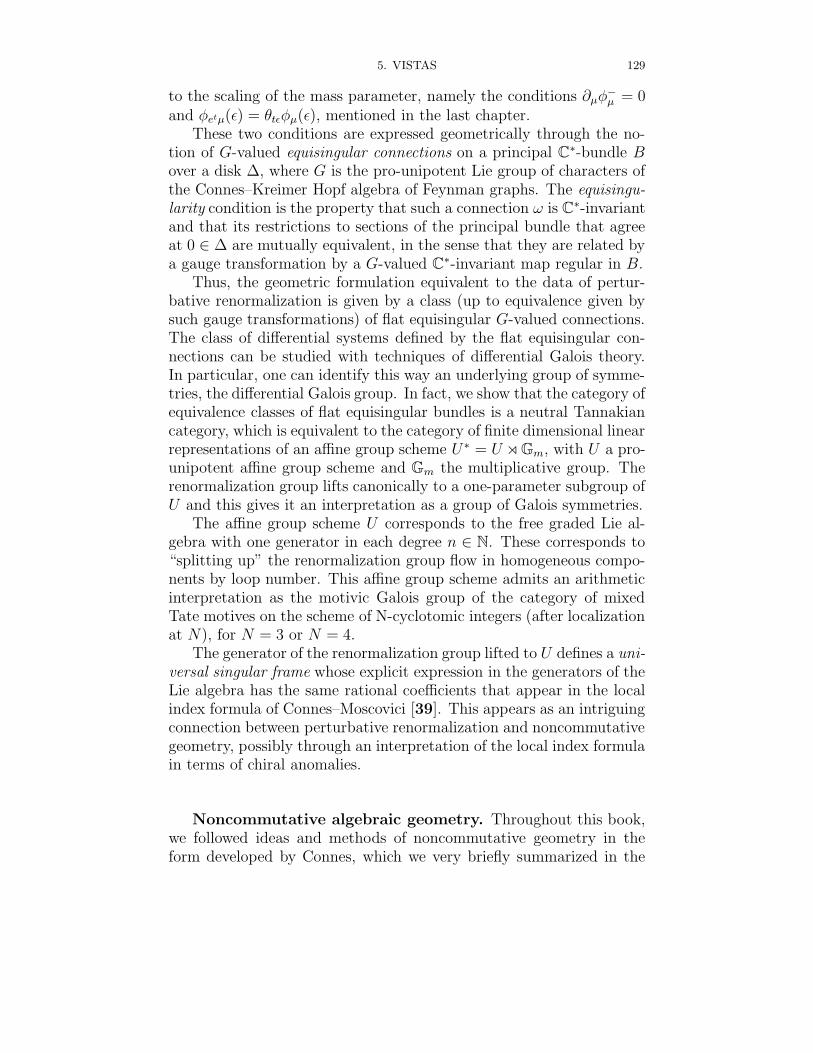
5. VISTAS 129
to the scaling of the mass parameter, namely the conditions ∂µφ−µ = 0
and φetµ(ε) = θtεφµ(ε), mentioned in the last chapter.These two conditions are expressed geometrically through the no-
tion of G-valued equisingular connections on a principal C∗-bundle Bover a disk ∆, where G is the pro-unipotent Lie group of characters ofthe Connes–Kreimer Hopf algebra of Feynman graphs. The equisingu-larity condition is the property that such a connection ω is C∗-invariantand that its restrictions to sections of the principal bundle that agreeat 0 ∈ ∆ are mutually equivalent, in the sense that they are related bya gauge transformation by a G-valued C∗-invariant map regular in B.
Thus, the geometric formulation equivalent to the data of pertur-bative renormalization is given by a class (up to equivalence given bysuch gauge transformations) of flat equisingular G-valued connections.The class of differential systems defined by the flat equisingular con-nections can be studied with techniques of differential Galois theory.In particular, one can identify this way an underlying group of symme-tries, the differential Galois group. In fact, we show that the category ofequivalence classes of flat equisingular bundles is a neutral Tannakiancategory, which is equivalent to the category of finite dimensional linearrepresentations of an affine group scheme U ∗ = U o Gm, with U a pro-unipotent affine group scheme and Gm the multiplicative group. Therenormalization group lifts canonically to a one-parameter subgroup ofU and this gives it an interpretation as a group of Galois symmetries.
The affine group scheme U corresponds to the free graded Lie al-gebra with one generator in each degree n ∈ N. These corresponds to“splitting up” the renormalization group flow in homogeneous compo-nents by loop number. This affine group scheme admits an arithmeticinterpretation as the motivic Galois group of the category of mixedTate motives on the scheme of N-cyclotomic integers (after localizationat N), for N = 3 or N = 4.
The generator of the renormalization group lifted to U defines a uni-versal singular frame whose explicit expression in the generators of theLie algebra has the same rational coefficients that appear in the localindex formula of Connes–Moscovici [39]. This appears as an intriguingconnection between perturbative renormalization and noncommutativegeometry, possibly through an interpretation of the local index formulain terms of chiral anomalies.
Noncommutative algebraic geometry. Throughout this book,we followed ideas and methods of noncommutative geometry in theform developed by Connes, which we very briefly summarized in the
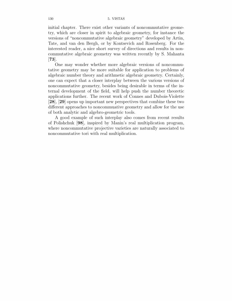
130 5. VISTAS
initial chapter. There exist other variants of noncommutative geome-try, which are closer in spirit to algebraic geometry, for instance theversions of “noncommutative algebraic geometry” developed by Artin,Tate, and van den Bergh, or by Kontsevich and Rosenberg. For theinterested reader, a nice short survey of directions and results in non-commutative algebraic geometry was written recently by S. Mahanta[73].
One may wonder whether more algebraic versions of noncommu-tative geometry may be more suitable for application to problems ofalgebraic number theory and arithmetic algebraic geometry. Certainly,one can expect that a closer interplay between the various versions ofnoncommutative geometry, besides being desirable in terms of the in-ternal development of the field, will help push the number theoreticapplications further. The recent work of Connes and Dubois-Violette[28], [29] opens up important new perspectives that combine these twodifferent approaches to noncommuative geometry and allow for the useof both analytic and algebro-geometric tools.
A good example of such interplay also comes from recent resultsof Polishchuk [98], inspired by Manin’s real multiplication program,where noncommutative projective varieties are naturally associated tononcommutative tori with real multiplication.
Bibliography
[1] N. Alling, N. Greenleaf, Foundations of the theory of Klein surfaces, LectureNotes in Mathematics Vol. 219, Springer Verlag 1971.
[2] L. Alvarez-Gaume, G. Moore, C. Vafa, Theta functions, modular invariance,and strings. Comm. Math. Phys. 106 (1986), no. 1, 1–40.
[3] S. Aminneborg, I. Bengtsson, D. Brill, S. Holst, P. Peldan, Black holes andwormholes in 2 + 1 dimensions, Class. Quantum Grav. 15 (1998) 627–644.
[4] J. Arledge, M. Laca, I. Raeburn, Semigroup crossed products and Heckealgebras arising from number fields, Doc. Math. 2 (1997) 115–138.
[5] K. I. Babenko, On a problem of Gauss. Dokl. Akad. Nauk SSSR, Tom 238(1978) No. 5, 1021–1024.
[6] J. D. Barrow. Chaotic behaviour and the Einstein equations. In: ClassicalGeneral Relativity, eds. W. Bonnor et al., Cambridge Univ. Press, Cam-bridge, 1984, 25–41.
[7] P. Baum, A. Connes, Geometric K-theory for Lie groups and foliations.Preprint IHES 1982; l’Enseignement Mathematique, t. 46, 2000, 1-35.
[8] F.P. Boca, Projections in rotation algebras and theta functions, Commun.Math. Phys. 202 (1999) 325–357.
[9] J.B. Bost, A. Connes, Hecke algebras, Type III factors and phase transitionswith spontaneous symmetry breaking in number theory, Selecta Math. (NewSeries) Vol.1 (1995) N.3, 411–457.
[10] R. Bowen, Hausdorff dimension of quasi–circles, Publ.Math. IHES 50 (1979)11–25.
[11] M. Boyle, D. Handelman, Orbit equivalence, flow equivalence, and orderedcohomology, Israel J. Math. 95 (1996) 169–210.
[12] O. Bratteli, D.W. Robinson, Operator algebras and quantum statistical me-chanics I,II, Springer Verlag, 1981.
[13] P. Chakraborty, A. Pal, Equivariant spectral triples on the quantum SU(2)group, K-Theory 28 (2003), no. 2, 107–126.
[14] C.H.Chang and D.Mayer, Thermodynamic formalism and Selberg’s zetafunction for modular groups, Regular and chaotic dynamics 15 (2000) N.3281–312.
[15] P.B. Cohen, A C∗-dynamical system with Dedekind zeta partition functionand spontaneous symmetry breaking, Journal de Theorie des Nombres deBordeaux 11 (1999) 15–30.
[16] A. Connes, C∗ algebres et geometrie differentielle. C.R. Acad. Sci. Paris,Ser. A-B , 290 (1980) 599–604.
[17] A. Connes, An analogue of the Thom isomorphism for crossed products of aC∗-algebra by an action of R, Adv. in Math. 39 (1981), no. 1, 31–55.
131
132 BIBLIOGRAPHY
[18] A. Connes, Non–commutative differential geometry, Publ.Math. IHES N.62(1985) 257–360.
[19] A. Connes, Cyclic cohomology and the transverse fundamental class of afoliation. In: Geometric methods in operator algebras (Kyoto, 1983). PitmanRes. Notes in Math., 123, Longman, Harlow 1986, 52–144.
[20] A. Connes, Compact metric spaces, Fredholm modules, and hyperfiniteness,Ergod. Th. Dynam. Sys. (1989) 9, 207–220.
[21] A. Connes, Noncommutative geometry, Academic Press, 1994.[22] A. Connes, Geometry from the spectral point of view. Lett. Math. Phys. 34
(1995), no. 3, 203–238.[23] A. Connes, Trace formula in Noncommutative Geometry and the zeros of
the Riemann zeta function. Selecta Mathematica. New Ser. 5 (1999) 29–106.[24] A. Connes, A short survey of noncommutative geometry, J. Math. Phys. 41
(2000), no. 6, 3832–3866.[25] A. Connes, Cyclic cohomology, Quantum group Symmetries and the Local
Index Formula for SUq(2), J. Inst. Math. Jussieu 3 (2004), no. 1, 17–68.[26] A. Connes, M. Douglas, A. Schwarz, Noncommutative geometry and Matrix
theory: compactification on tori. J. High Energy Phys. (1998) no. 2, Paper3, 35 pp. (electronic)
[27] H. Darmon, Rational points on modular elliptic curves, CBMS RegionalConference Series in Mathematics, 101. American Mathematical Society,2004.
[28] A. Connes, M. Dubois-Violette, Noncommutative finite-dimensional man-ifolds. I. spherical manifolds and related examples, Comm. Math. Phys.Vol.230 (2002) N.3, 539–579.
[29] A. Connes, M. Dubois-Violette, Moduli space and structure of noncommu-tative 3-spheres, Lett. Math. Phys., Vol.66 (2003) N.1-2, 91–121.
[30] A. Connes, D. Kreimer, Renormalization in quantum field theory and theRiemann-Hilbert problem. I. The Hopf algebra structure of graphs and themain theorem. Comm. Math. Phys. 210 (2000), no. 1, 249–273.
[31] A. Connes, D. Kreimer, Renormalization in quantum field theory andthe Riemann-Hilbert problem. II. The β-function, diffeomorphisms and therenormalization group. Comm. Math. Phys. 216 (2001), no. 1, 215–241.
[32] A. Connes, M. Marcolli, Quantum Statistical Mechanics of Q-lattices, (FromPhysics to Number Theory via Noncommutative Geometry, Part I), preprintarXiv:math.NT/0404128.
[33] A. Connes, M. Marcolli, Q-lattices: quantum statistical mechanics and Ga-lois theory, to appear in Journal of Geometry and Physics.
[34] A. Connes, M. Marcolli, Renormalization and motivic Galois theory, Int.Math. Res. Not. 2004, no. 76, 4073–4091.
[35] A. Connes, M. Marcolli, Renormalization, the Riemann-Hilbert correspon-dence, and motivic Galois theory (From Physics to Number Theory via Non-commutative Geometry. Part II), preprint arXiv hep-th/0411114.
[36] A. Connes, M. Marcolli, Quantum fields and motives, to appear in Journalof Geometry and Physics.
[37] A. Connes, M. Marcolli, Noncommutative Geometry from Quantum Physicsto Motives, book in preparation.
BIBLIOGRAPHY 133
[38] A. Connes, M. Marcolli, N. Ramachandran KMS states and complex multi-plication, arXiv math.OA/0501424
[39] A. Connes, H. Moscovici, The local index formula in noncommutative geom-etry. Geom. Funct. Anal. 5 (1995), no. 2, 174–243.
[40] A. Connes, H. Moscovici, Cyclic cohomology and Hopf algebras, Lett. Math.Phys. 48 (1999), no. 1, 97–108.
[41] A. Connes, H. Moscovici, Modular Hecke algebras and their Hopf symmetry,Moscow Math. Journal, Vol.4 (2004) N.1, 67–109.
[42] A. Connes, H. Moscovici, Rankin-Cohen Brackets and the Hopf Algebra ofTransverse Geometry, Moscow Math. Journal, Vol.4 (2004) N.1, 111–130.
[43] C. Consani, Double complexes and Euler L–factors, Compositio Math. 111(1998) 323–358.
[44] C. Consani, M. Marcolli, Noncommutative geometry, dynamics and ∞-adicArakelov geometry, to appear in Selecta Mathematica
[45] C. Consani, M. Marcolli, Triplets spectreaux in geometrie d’Arakelov,C.R.Acad.Sci. Paris, Ser. I 335 (2002) 779–784.
[46] C. Consani, M. Marcolli, New perspectives in Arakelov geometry, to appearin proceedings of CNTA7 meeting Montreal 2002.
[47] C. Consani, M. Marcolli, Spectral triples from Mumford curves, InternationalMathematics Research Notices 36 (2003) 1945–1972.
[48] C. Consani, M. Marcolli, Archimedean cohomology revisited, arXivmath.AG/0407480.
[49] C. Consani, M. Marcolli (editors), Proccedings of the conference “Noncom-mutative geometry and number theory” held in Bonn 2003. To appear.
[50] G. Cornell and J.H. Silverman (eds.) Arithmetic geometry, Springer-Verlag,New York, 1986
[51] J. Cuntz, W. Krieger, A class of C∗–algebras and topological Markov chains,Invent. Math. 56 (1980) 251–268.
[52] C. Deninger, On the Γ–factors attached to motives, Invent. Math. 104 (1991)245–261.
[53] C. Deninger, Local L-factors of motives and regularized determinants. Invent.Math. 107 (1992), no. 1, 135–150.
[54] C. Deninger, Motivic L-functions and regularized determinants, in “Mo-tives”, Proceedings of Symposia in Pure Mathematics, Vol. 55 (1994) PartI, 707–743.
[55] V. Drinfeld, Two theorems on modular curves, Funct. Anal. and its Appli-cations, Vol.7 (1973) N.2, 155–156.
[56] V. Drinfeld, Yu.I. Manin, Periods of p-adic Schottky groups. J. Reine Angew.Math. 262/263 (1973), 239–247.
[57] E. Ha, F. Paugam, private communication.[58] R. Haag, Local Quantum Physics, Springer, Berlin 1992.[59] R. Haag, N. M. Hugenholtz, M. Winnink On the equilibrium states in quan-
tum statistical mechanics, Comm. Math. Phys. 5 (1967), 215, 236.[60] D. Harari, E. Leichtnam, Extension du phenomene de brisure spontanee
de symetrie de Bost–Connes au cas des corps globaux quelconques, SelectaMath. (New Series) Vol.3 (1997) 205–243.
134 BIBLIOGRAPHY
[61] G. Harder, General aspects in the theory of modular symbols, Seminar onnumber theory, Paris 1981–82 (Paris, 1981/1982), 73–88, Progr. Math., 38,Birkhauser Boston, Boston, MA, 1983.
[62] D. Hensley, Continued fraction Cantor sets, Hausdorff dimension, and func-tional analysis, J. Number Theory 40 (1992) 336–358.
[63] I. M. Khalatnikov, E. M. Lifshitz, K. M. Khanin, L. N. Schur, Ya. G. Sinai.On the stochasticity in relativistic cosmology. J. Stat. Phys., 38:1/2 (1985),97–114.
[64] M. Khalkhali, B. Rangipour, Introduction to Hopf-Cyclic Cohomology,preprint, arXiv math.QA/0503244.
[65] K. Krasnov, Holography and Riemann Surfaces, Adv. Theor. Math. Phys. 4(2000) 929–979
[66] K. Krasnov, Analytic Continuation for Asymptotically AdS 3D Gravity, gr-qc/0111049
[67] M. Laca, Semigroups of ∗-endomorphisms, Dirichlet series, and phase tran-sitions. J. Funct. Anal. 152 (1998), no. 2, 330–378.
[68] M. Laca, From endomorphisms to automorphisms and back: dilations andfull corners, J. London Math. Soc. (2) 61 (2000) 893–904.
[69] S. Lang, Elliptic Functions, (Second Edition), Graduate Texts in Mathemat-ics, Vol.112, Springer-Verlag 1987.
[70] G. Landi, An introduction to noncommutative spaces and their geometries,Lecture Notes in Physics, Vol. m-51, Springer Verlag 1997.
[71] S. Lang, Introduction to Arakelov Theory, Springer-Verlag, New York, 1988.[72] R. Loudon, The Quantum Theory of Light, third edition, Oxford University
Press, 2000.[73] S. Mahanta, A Brief Survey of Non-Commutative Algebraic Geometry,
preprint arXiv math.QA/0501166.[74] L. Mandel, E. Wolf, Optical Coherence and Quantum Optics, Cambridge
University Press, 1995.[75] Yu.I. Manin, Von Zahlen und Figuren, arXiv math.AG/0201005.[76] Yu.I. Manin, Real Multiplication and noncommutative geometry, arXiv
math.AG/0202109.[77] Yu.I. Manin, Theta functions, quantum tori, and Heisenberg groups, Lett.
in Math. Phys. 56 (2001) 295–320.[78] Yu.I. Manin, Lectures on zeta functions and motives (according to Deninger
and Kurokawa). Columbia University Number Theory Seminar (New York,1992). Asterisque No. 228 (1995), 4, 121–163.
[79] Yu.I. Manin, Three–dimensional hyperbolic geometry as ∞–adic Arakelovgeometry, Invent. Math. 104 (1991) 223–244.
[80] Yu.I. Manin, p-adic automorphic functions. Journ. of Soviet Math., 5 (1976)279-333.
[81] Yu.I. Manin, Parabolic points and zeta functions of modular curves, Math.USSR Izvestija, vol. 6 N. 1 (1972) 19–64. Selected Papers, World Scientific,1996, 202–247.
[82] Yu.I. Manin, M. Marcolli, Holography principle and arithmetic of algebraiccurves, Adv. Theor. Math. Phys. Vol.3 (2001) N.5, 617–650.
BIBLIOGRAPHY 135
[83] Yu.I. Manin, M. Marcolli, Continued fractions, modular symbols, and non-commutative geometry, Selecta Mathematica (New Series) Vol.8 N.3 (2002)475-520.
[84] M. Marcolli, Limiting modular symbols and the Lyapunov spectrum, Journalof Number Theory, Vol.98 N.2 (2003) 348-376.
[85] M. Marcolli, Modular curves, C∗-algebras and chaotic cosmology, arXivmath-ph/0312035.
[86] K. Matsuzaki, M. Taniguchi, Hyperbolic manifolds and Kleinian groups, Ox-ford Univ. Press, 1998.
[87] D.H. Mayer, Relaxation properties of the mixmaster universe, Phys. Lett. A121 (1987), no. 8-9, 390–394.
[88] D.H. Mayer, Continued fractions and related transformations, in “ Ergodictheory, symbolic dynamics, and hyperbolic spaces”, Oxford Univ. Press,1991.
[89] B. Mazur, Courbes elliptiques et symboles modulaires, Seminaire Bourbakivol.1971/72, Exposes 400–417, LNM 317, Springer Verlag 1973, pp. 277–294.
[90] L. Merel, Intersections sur les courbes modulaires, Manuscripta Math., 80(1993) 283–289.
[91] J.S. Milne, Canonical models of Shimura curves, manuscript, 2003 (availablefrom www.jmilne.org)
[92] D. Mumford (with M.Nori and P.Norman), Tata lectures on theta, III,Progress in Mathematics Vol. 97, Birkhauser 1991.
[93] D. Mumford, An analytic construction of degenerating curves over completelocal rings, Compositio Math. 24 (1972) 129–174.
[94] D. Mumford, C. Series, D. Wright, Indra’s Pearls. The Vision of Felix Klein.Cambridge University Press, New York, 2002.
[95] W. Parry, S. Tuncel, Classification problems in ergodic theory, London Math.Soc. Lecture Notes Series 67, 1982.
[96] F. Paugam, Three examples of noncommutative boundaries of Shimura va-rieties, preprint arXiv math.AG/0410254.
[97] F. Paugam, Quelques bords irrationnels de varietes de Shimura, preprintarXiv math.AG/0410269.
[98] A. Polishchuk, Noncommutative two-tori with real multiplication as noncom-mutative projective varieties, J. Geom. Phys. 50 (2004), no. 1-4, 162–187.
[99] M. Pollicott, H. Weiss, Multifractal analysis of Lyapunov exponent for con-tinued fraction and Manneville-Pomeau transformations and applications toDiophantine approximation, Comm. Math. Phys. 207 (1999), no. 1, 145–171.
[100] D.B. Ray, I.M. Singer, Analytic torsion for complex manifolds. Ann. of Math.(2) 98 (1973), 154–177.
[101] M.A. Rieffel, C∗-algebras associated to irrational rotations, Pacific J. Math.93 (1981) 415-429.
[102] A.L. Rosenberg, Noncommutative schemes. Compositio Math. 112 (1998)N.1, 93–125.
[103] J.P. Serre, Facteurs locaux des fonctions zeta des varietes algebriques(definitions et conjectures). Sem. Delange-Pisot-Poitou, exp. 19, 1969/70.
[104] G. Shimura, Arithmetic Theory of Automorphic Functions, Iwanami Shotenand Princeton 1971.
136 BIBLIOGRAPHY
[105] H.M. Stark, L-functions at s = 1. IV. First derivatives at s = 0, Adv. Math.35 (1980) 197–235.
[106] P. Stevenhagen, Hilbert’s 12th problem, complex multiplication and Shimurareciprocity, Advanced Studies in Pure Math. 30 (2001) “Class Field Theory– its centenary and prospect” pp. 161–176.
[107] A. Weil, Basic Number Theory, Springer 1974.[108] R.O. Wells, Differential analysis on complex manifolds. Springer–Verlag,
1980.[109] A. Werner, Local heights on Mumford curves. Math. Ann. 306 (1996), no. 4,
819–831.[110] D. Zagier, Modular forms and differential operators, in K. G. Ramanathan
memorial issue. Proc. Indian Acad. Sci. Math. Sci. 104 (1994), no. 1, 57–75.