Lectures in International Finance - UNITE · Lectures in International Finance Giovanni Piersanti...

Lectures in International Finance

Giovanni PiersantiUniversity of Teramo and University of Rome Tor Vergata

January, 2016

Contents

I The Foreign Exchange Market 7

1 Market Institutions and Exchange Rates 91.1 Introduction . . . . . . . . . . . . . . . . . . . . . . . . . 91.2 The Markets for Foreign Exchange . . . . . . . . . . . . 101.3 Characteristics, Activities and Players . . . . . . . . . . 11

2 The Exchange Rates 172.1 Introduction . . . . . . . . . . . . . . . . . . . . . . . . . 172.2 The Spot Exchange Rate . . . . . . . . . . . . . . . . . . 172.3 The Forward Exchange Rate . . . . . . . . . . . . . . . . 212.4 Nominal, Real and E¤ective Exchange Rates . . . . . . . 26

3 Currency Derivatives and Options Markets 313.1 Introduction . . . . . . . . . . . . . . . . . . . . . . . . . 313.2 Futures . . . . . . . . . . . . . . . . . . . . . . . . . . . 323.3 Options . . . . . . . . . . . . . . . . . . . . . . . . . . . 323.4 Swaps . . . . . . . . . . . . . . . . . . . . . . . . . . . . 32

II The Balance of Payments Accounts 33

4 Balance-of-Payments and International Investment Po-sition 354.1 Introduction . . . . . . . . . . . . . . . . . . . . . . . . . 354.2 System Structure and Accounting Principles . . . . . . . 364.2.1 Accounting Principles . . . . . . . . . . . . . . . . . . 364.2.2 Standard Components . . . . . . . . . . . . . . . . . . 38

5 Some Linkages between BP, IIP, and National Accounts 455.1 Introduction . . . . . . . . . . . . . . . . . . . . . . . . . 455.2 Balance of Payments and National Accounts . . . . . . . 46

3

4 CONTENTS

III The Theory of Exchange Rates 53

6 Some Fundamental International Parity Conditions 556.1 The Purchasing Power Parity Principle . . . . . . . . . . 556.2 The Interest Parity . . . . . . . . . . . . . . . . . . . . . 57

7 Exchange Rate and Balance of Payments 637.1 Introduction . . . . . . . . . . . . . . . . . . . . . . . . . 637.2 The Elasticity Approach . . . . . . . . . . . . . . . . . . 637.3 The Absorption Approach . . . . . . . . . . . . . . . . . 677.4 The Multiplier Approach . . . . . . . . . . . . . . . . . . 707.5 The Interest Rates and the Capital Account . . . . . . . 73

8 Models of Exchange Rate Determination 758.1 Introduction . . . . . . . . . . . . . . . . . . . . . . . . . 758.2 The Monetary Model . . . . . . . . . . . . . . . . . . . . 758.3 Sticky Prices and Exchange-Rate Overshooting: the Dorn-

busch Model . . . . . . . . . . . . . . . . . . . . . . . . 878.4 The Portfolio Balance Model . . . . . . . . . . . . . . . 958.4.1 The Short-Run Equilibrium . . . . . . . . . . . . . . . 998.4.2 The Long-Run Equilibrium . . . . . . . . . . . . . . . 1038.5 Appendix . . . . . . . . . . . . . . . . . . . . . . . . . . 107

Preface

5

6 PREFACE

Part I

The Foreign ExchangeMarket

7

Chapter 1

Market Institutions and Ex-change Rates

1.1 Introduction

In a world where consumption, production, investment and capital mar-kets are globalized, international �nance, or international monetaryeconomics has become an integral part of any study of internationaleconomics.When studying international �nance which is, broadly speaking,

concerned with the monetary and macroeconomic relations betweencountries, a number of special problems arise. Many of these prob-lems are due to the use of di¤erent currencies in di¤erent countriesand the consequent need to exchange them. Rates of exchange be-tween currencies are set by a variety of arrangements and both ratesand arrangements are subject to change. Furthermore, exchange-ratechanges can have sizable e¤ects on balance-of-payments, economic ac-tivity, and policy strategy of the countries involved.In this chapter, we look at some preliminary issues. We examine

the operation of the key market without which no foreign transaction ispossible: the foreign exchange market. We introduce the terminologyused in foreign markets and discuss the basic structure and forces thatoperate in the market. We then examine the di¤erent type of transac-tions and the main �nancial instruments that are managed in currencymarkets.

9

10 Market Institutions and Exchange Rates

1.2 TheMarkets for Foreign Exchange

The foreign exchange, or forex (FX) market is the market where ex-change rates are determined. An exchange rate is a price, speci�callythe price of one currency in terms of another. It is the mechanismby which world currencies are tied together in the global marketplace.There are two common ways of expressing it. One, also referred toas price quotation system or direct quotation, expresses the exchangerate as the price of foreign currency in terms of domestic currency, i.e.,as the amount of domestic currency needed to purchase one unit of aforeign currency. The other, also known as volume quotation system orindirect quotation, expresses the exchange rate as the price of domes-tic currency in terms of foreign currency, i.e., as the amount of foreigncurrency required to purchase one unit of domestic currency. Note thatthe indirect quotation is just the reciprocal of the corresponding directquotation.1 In this book we will use the former quotation. Hence,unless otherwise stated, we de�ne the exchange rate as the price of do-mestic currency in terms of foreign currency. This implies that a rise(decrease) in the exchange rate means a depreciation (appreciation)of the domestic currency. For example, a rise in the dollars per eurofrom $1.101/e1 to $1.202/e1, means that the dollar has depreciatedin value, whereas a decrease from $1.101/e1 to $0.998/e1 means thatthe dollar appreciated in value. The opposite obviously holds if weused the indirect quotation.For the purpose of this chapter we refer to the foreign exchange, or

currency market as a single worldwide market where the currencies ofdi¤erent countries are exchanged or traded. However, its major opera-tors buy and sell foreign exchange from computer terminals which are

1Most currencies in the world are stated in terms of the number of units offoreign currency needed to buy one dollar. This quote, called "European" quote,expresses the rate as the foreign currency price of one U.S. dollar. For example,the exchange rate between U.S. dollars and Japanese yen is normally stated:

JPY122:816=$1;

read as "122.816 Japanese yen per dollar". An alternative method, called" Amer-ican" quote, states foreign exchange rates as the U.S. dollar price of one unit offoreign currency. The same exchange rate above expressed in American terms is:

$0:00814=JPY1;

read as �0.00814 dollars per Japanese yen". Note that European quote and Amer-ican quote are reciprocals:

1

JPY122:816=$1= $0:00814=JPY1:

Market Institutions and Exchange Rates 11

physically located all around the world. The foreign exchange marketis open 24 hours a day, split over three time zones. Trading begins eachday in Sydney, and moves around the world as the business day beginsin each �nancial center, �rst to Tokyo, then to London, and New York.The foreign exchange market has no physical venue where traders meetto deal in currencies. Computer screens around the world do the job,continuously showing exchange rate prices to traders so that they candeal with each other and �nd people willing to meet that price. It doesnot matter where the counterparties are located, if in London, Singa-pore, New York, Tokyo, Zurich, or Frankfurt. What matter is simplythe willing to meet that price. There are, therefore, distinct FXmarketsin the real world, although they are linked by arbitrage, a mechanismensuring that the rate of exchange between currencies quoted in di¤er-ent markets (i.e., in London, Tokyo, and other international �nancialcenter) be the same. The process of arbitrage is discussed below andjustify the convention we followed here to talk about the forex marketas a single market covering the whole world.

1.3 Characteristics, Activities andPlayers

The forex market is the most liquid and largest �nancial market inthe world. According to the Triennial Central Bank Survey carriedout by the Bank for International Settlements (BIS), the trading inforeign exchange markets averaged $5.3 trillion per day in April 2013.2

The daily average volume was about ten times the daily volume of allthe world�s equity markets and sixty times the U.S. daily GDP. TheUS dollar remained the dominant vehicle currency: it was involved in87% of all trades in April 2013. The euro was the second most tradedcurrency (33%), followed by the Japanese yen (23%), and the Britishpound (12%). Several emerging market currencies, and the Mexicanpeso and Chinese renminbi entered the list of the top 10 most tradedcurrencies.Trading was increasingly concentrated in the largest �nancial cen-

tres. In April 2013, sales desks in the United Kingdom, the UnitedStates, Singapore and Japan intermediated 71% of foreign exchangetrading, whereas the major markets in the European Union (Frank-furt, Paris, and Amsterdam) played a smaller role.Given the international nature of the market, the majority (57%)

2See BIS (2013).


of all foreign exchange transactions involved cross-border counterpar-ties. This highlights one of the main concerns in the foreign exchangemarket: counterparty risk.Foreign exchange is an over-the-counter (OTC) market where bro-

kers/dealers negotiate directly with one another, so there is no centralexchange or clearing house.The main activities in the FX markets are speculation and arbi-

trage, foreign assets and international trade �nancing, hedging.

Speculation and arbitrageSpeculation and arbitrage are both �nancial strategies used by traders,to make larger pro�ts. However, the technique in which each strategyis used di¤ers substantially.In a typical speculation activity, a trader takes on a foreign exchange

position on the expectation of a favorable currency rate change. Forexample, a trader may open a long position on a currency (i.e., buythe currency today) with the expectation of pro�ting from a futureappreciation (i.e., sell the currency at a higher price in the future). Ifthe currency appreciates, the trader may close the trade for a pro�t.Conversely, if the currency depreciates, the trade might be closed for aloss. A speculator who expects a currency to appreciate in the futureis said to be bullish.Speculators, on the other hand, may open a short position (i.e.,

selling short, or simply selling the currency today in the hope of buyingit back at a lower rate in the future) if they expect the currency todepreciate. If the currency drop, the position will be pro�table. If thecurrency rise, the trade may be closed at a loss. A speculator whoexpects a currency to depreciate in the future is said to be bearish.Speculation, therefore, is a type of �nancial strategy that involves

a signi�cant amount of risk.Arbitrage, on the other hand, is a riskless trading strategy that

allows traders to take advantage of price di¤erentials prevailing simul-taneously in di¤erent markets and across currencies. The simplest formof arbitrage in the FX market is spatial arbitrage, which takes advan-tage of the pricing discrepancies across geographically separate mar-kets. For example, if the dollar-euro exchange rate quoted in New Yorkis $1.101/e1 but $1.085/e1 in London, it would pay the traders to buyeuros in London and simultaneously sell them in New York, making arisk-free pro�t of 1.6 cents on every euro bought and sold. This activitywill make the euro to appreciate in London and to depreciate in NewYork, leading to an arbitrage-free equilibrium where the rate quotedin the two centers are equal.3 Cross-currency, or triangular arbitrage

3Notice that all the examples discussed here imply zero transaction costs. These


takes advantage of discrepancies in the cross rates of di¤erent currencypairs. To illustrate suppose that the dollar-euro rate is $1.085/e1, andthe pound-euro rate is £ 0.695/e1. The implied outright rate betweenthe pound and the dollar is thus $1.561/£ 1=($1.085/e1)/(£ 0.695/e1).If the actual pound-euro rate is instead £ 0.682/e1, implying a rateof $1.591/£ 1=($1.085/e1)/(£ 0.682/e1), then a dealer wanting dollarswould do better to �rst sell euros for pound, e.g., selle1,000�0.682=£ 682,and then sell pound for dollars obtaining $1,085.062=£ 682�1.591 foran arbitrage pro�t of $1,085.062-$1,000=$85.062. Covered interest ar-bitrage takes advantage of a misalignment of spot and forward rates(which you will learn about in the next section), and domestic andforeign interest rates.

Foreign assets and international trade �nancingForeign assets and international trade �nancing is overwhelmingly themajor business of forex markets. It allows individuals and �rms con-ducting international business (e.g., importers and exporters, compa-nies making direct foreign investments, international investors buyingor selling debt or equity investments for their portfolios) to transferpurchasing power from one country and its currency to another, alterthe structure of assets and liabilities in di¤erent countries, obtain orprovide credit for international economic transactions.

HedgingHedging is a way used by companies, �nancial investors and othereconomic agents to insure against the foreign exchange risk resultingin all international transactions. Hence, by contrast to speculation,hedging is the activity of covering an open position. By using thisstrategy properly, a trader who is long on a particular foreign currency(orders to buy or book a �xed amount of a foreign currency) can beprotected from downside risk (a downward price move), while a traderwho is short on a particular foreign currency (orders to sell a �xed

are costs incurred when buying or selling currencies. Transaction costs include bro-kers/dealers commissions and spreads. Spread, or bid-ask spread is the di¤erencebetween the buying and selling price of a given currency which exists at the samemoment in the forex markets. It represents the gross pro�t margin of the bro-ker/dealer. In quotations on the foreign markets bids always precede asks. Forexample, if the quote for the dollar-euro rate is 1:08278 � 1:08313, 1:08278 is thebid, or buying price (i.e., the rate at which a trader will purchase the dollar) and1:08313 is the ask, or selling price (i.e., the rate at which a trader will sell thedollar). Hence, in this case the bid-ask spread is 1:08313� 1:08278 = 0:00035, andthe gross pro�t margin of the broker/dealer is 0; 032% = (0:00035=1:08313) � 100of the traded amount of dollars.


amount of a foreign currency) can be protected against upside risk (aupward price move).The main players in the market are speculators and arbitragers,

commercial and investment banks, foreign exchange brokers, retailclients, and central banks.

Speculators and arbitragersSpeculators and arbitragers are businesses, international investors, multi-national corporations and other who seek to pro�t from trading in themarket.

Commercial and investment banksThese are leading players who buy and sell currencies from each otherwithin what is known as the interbank market. Commercial and invest-ment banks not only trade for their customers and on their own behalfthrough proprietary desks (proprietary trading), but also provide thechannel through which all other market participants must trade. Theyaccount for by far the largest proportion of total trading volume, thusplaying the vital role of catalysts in international �nancial markets.

Foreign exchange brokersForex brokers are intermediaries that make it easier to connect tradersin the interbank market. Typically, a forex broker o¤er quotationsfor most currency from the banks that they have relationships with,showing the best rates. There is a small cost a trader is likely to incurwhen dealing through a broker. This is known as a brokerage fee, whichis a commission charged by brokers for every currency pair they o¤eron their trading platform.

Retail clientsThese are made up of consumers and travellers, businesses, investorsand others who need foreign currencies for their personal and businesspurposes. They normally do not buy and sell currencies directly withone another, rather they operate with brokers and commercial banks.

Central banksThese are institutions to which the management of exchange rates andforeign reserves (see, Section ) is attributed. Central banks play a veryimportant role in foreign exchange market. However, they normally


do not undertake a signi�cant volume of trading. They enter the FXmarkets to trade with other central banks, various international insti-tutions, and to maintain �nancial stability in the exchange rate.

Chapter 2

The Exchange Rates

2.1 Introduction

In the previous section we referred to �the exchange rate�as the relativeprice of two currencies. Yet, the use of the singular noun is a simpli�ca-tion, which disguises the fact that in reality a variety of exchange ratesexists at the same moment between the same two currencies. There areexchange rates for cash, or bank notes; exchange rates for checks andfor electronic payments (credit card); exchange rates for the purchase orsale of a foreign currency. These rates can di¤er because of transactioncosts, carrying (storage and custody) costs, bid-ask spreads, brokeragefees. The di¤erences are however very small, so that henceforth weshall argue as if there is only one exchange rate for each foreign cur-rency. Nevertheless, there is still a set of rates for each currency whichwe cannot ignore.We start by looking at the di¤erence between the spot and forward

exchange rates.

2.2 The Spot Exchange Rate

The spot, or current exchange rate is the rate paid for immediate de-livery of a currency. Except for certain cases such as an exchangeof banknotes, normally "immediate delivery" means settlement of the

17

18 The Exchange Rates

foreign-exchange contract within two business days.

Figure 1.1 Exchange-rate equilibrium in the spot market

The spot exchange rate is determined in the spot market whichis made up of �nancial institutions (e.g., commercial and investmentbanks, pension funds, hedge funds, money market funds, insurancecompanies, �nancial government entities) and non-�nancial institutions(e.g., corporations, non-�nancial government entities, private individ-uals) involved in buying and selling foreign currencies. According toBIS (2013) Triennial Survey, in 2013 the daily volume of spot contractswas $1.759 trillion (38% of total turnover). The majority of the spottrading was between �nancial institutions; only 19 percent of the dailyspot transactions involved non-�nancial customers. This market is cel-ebrated for the phrenetic rate at which it runs and the huge amountof money which is moved at a lighting speed in response to very smallchanges in price quotations.Like in any other market, the demand for and supply of foreign ex-

change determine the price of a currency in the spot market, as shownin Figure 1.1. The �gure describes a very simple (partial equilibrium)model of exchange-rate determination which serves as a useful intro-duction to the more general and complete models discussed in the nextchapters.

The Exchange Rates 19

In Figure 1.1 we display the amount of a foreign currency (FC) onthe horizontal axis and the price, or exchange rate of that currency (S)on the vertical axis. Both supply and demand curves are plotted aswell-behaved functions of the currency price, i.e., as increasing with theexchange rate for the supply function SFC(S), and decreasing with itsprice for the demand function DFC(S). In reality, there is no warrantythat these functions are well-behaved. In particular, a real possibilitythat a currency supply curve slopes downward exits, rising the criticalissue of explaining why foreign exchange markets are unstable. Weshall examine this issue in Chapter , Section . Hence, in order topreserve simplicity we here overlook the conditions for exchange ratestability. For now you simply note that the odd case of a downward-sloping supply arise because on the horizontal axis we display values(e.g., the amount of euros, or dollars, or yen, etc.) and not quantities(e.g., number of cars, or phones, or wine bottles, etc.) as in traditionalsupply and demand setup. Values involve prices and quantities andthey respond di¤erently than do quantities (see ).The supply and demand curves of a foreign currency derive from

the �ow of payments between the residents of a country and the restof world during a given time period. These �ows are summarized inthe balance-of-payments account, which records the country�s interna-tional transactions with other nations (see Chap. 4). To understand,let us consider the supply curve �rst. It comes from the need by foreignresidents to buy the domestic currency with foreign currency to pay fortheir purchases in the domestic country, i.e., to pay for domestic ex-ports, holding of domestic assets, traveling to the domestic country.Being the exchange rate here de�ned as the price of domestic currencyin terms of foreign currency (i.e., as the amount of domestic currencyneeded to purchase one unit of a foreign currency), a rise (depreciation)in S means that domestic exports, assets, travelling and tourism be-come cheaper for foreign residents. As such, they will start purchasingmore domestic goods, assets and services, therefore leading to an in-creased demand of domestic currency which is purchased by increasingthe supply of foreign currency. This yields an upward-sloping supplycurve in the [FC; S] plan.To take a simple example, let us look at the euro-dollar exchange

rate (e/$), and imagine that the euro depreciates against the dollarmoving from e0.903/$1 to e0.982/$1. Following the euro depreciation,the cost of EUR exports turns out to be cheaper for US resident andthis will increase the demand for EUR exports and hence for euroswhich are purchased by increasing the amount of dollars supplied inthe forex market. As a result, the supply curve for dollars happens toslope upward in the foreign exchange market.Similarly, the demand curve for a foreign currency derives from


domestic residents purchasing foreign goods and services, i.e., domesticimports, domestic investors purchasing foreign assets, and domestictourists traveling abroad. In this case, a rise in S means that importsbecomes costlier for domestic residents, leading to a reduced demandof foreign goods and with it to a reduced demand of foreign currency.This results in a downward-sloping demand curve in the [FC; S] plan.

Figure 1.2 The e¤ects of changes in demand and supply

In the example given above, a depreciation of the euro against thedollar makes the price of US exports to EUR importers to rise and thisleads to a lower demand for US exports and hence dollars. Therefore,the demand curve for dollars slopes downward in the forex market.Under a �exible exchange-rate regime, currency market equilibrium

is found at a price such that the supply of and the demand for theforeign currency are equal. This is S� in Figure 1.1. Exchange ratesother than S� cannot be sustained in the market, as they will tend tofall (appreciate) if there is an excess supply (S1 in Fig.1.1) and to rise(depreciate) if there is an excess demand (S2 in Fig.1.1).1 It also followsfrom Figure 1.1 that any factor which results in a shift in the demand

1Under a �xed rate regime, on the other hand, the foreign exchange value of acurrency is deliberately set by the government authorities, who actively act in themarket to keep the �xed rate from changing. Alternative exchange-rate regimes arediscussed in Chapter


for or supply of the foreign currency will result in price changes until anew equilibrium level is secured. These equilibrium price changes areshown in Figure 1.2.

2.3 The Forward Exchange Rate

The forward exchange rate is the rate that is agreed today for deliveryof a currency at some future date. The rate is negotiated and settledat the time the contract is made but payment and delivery are notrequired until maturity. Banks typically quote forward rates for valuedates of 1 month (30 days), 2 months (60 days), 3 months (90 days),6 months (180 days), 9 months (270 days) and 12 months (360 days).However, actual contracts can be arranged for other lengths up to 5 or10 years.The forward exchange market is valuable for three main classes of

activity, hedging, arbitrage and speculation. As stressed in Sect. 2.1,hedging is the activity of ensuring against the exchange risk comingfrom possible future �uctuations in the spot exchange rate. For exam-ple, an importer (exporter) who has to make (is to receive) a paymentin foreign currency at a given future date can ensure himself against theexchange rate risk by buying (selling) the necessary amount of foreigncurrency in the forward market. Since the exchange rate is �xed now,he then knows exactly how much he will pay (receive) in domestic cur-rency. Arbitrage and speculation are the activity of taking advantageof interest-rate and price di¤erentials in the forward and spot market.For example, if a speculator believes a given foreign currency will ap-preciate in the future, he will buy that currency in the forward market.When the contract matures he will sell the currency on the spot mar-ket to make a pro�t (if he got it right). Similar considerations hold forarbitraging as we show below.Forward contracts, in any case, are not the only way of carrying out

these activities. Another possibility is to use the spot market. There-fore, the issue of which market is the best alternative arise naturally.We shall look at this question by considering the case of an economic

agent who need a foreign currency to make a payment at a future date,or to invest in foreign bonds, or to speculate.2 For simplicity, let usfocus on a one-period-forward market and denote the correspondingforward rate as Ft;t+1, where t and t+1 are the day the forward contract

2The case of an agent who expects a payment at a future date is a mirror-imageof this.


is negotiated and the day it is executed, respectively.3 In addition, letA, St, it and i�t be the amount of foreign currency due in the future,the date t spot exchange rate, and the one-period date t domestic andforeign interest rates, respectively. Under this conditions, the availablealternative are as follows:

� the agent can buy the sum A on the forward market paying outnext period Ft;t+1A in domestic currency (forward covering);

� the agent can use the spot market to purchase an amountA= (1 + i�t )of foreign currency, invest it in the foreign country at the inter-est rate i�t for one period to obtain [A= (1 + i�t )] (1 + i�t ) = Aat the maturity date (spot covering). The cost of A= (1 + i�t )on the spot market is StA= (1 + i�t ); the opportunity cost (in-terest foregone on owned funds, or paid on borrowed funds) is[StA= (1 + i�t )] (1 + it).

It then follows that the �rst alternative is better than, the same as,or worse than the second one according to whether

Ft;t+1A SStA1 + it1 + i�t

; (1.1)

that is, according to whether forward covering is cheaper, cost the sameas, or is costlier than spot covering.An alternative strategy called currency swap is to buy the foreign

currency spot and sell it forward (swap-in), or sell the foreign currencyspot and buy it forward (swap-out). More generally, a swap is anagreement to buy, or borrow and sell, or lending foreign exchange ata �xed exchange rate where the buying and selling are separated intime.4

Nevertheless, as long as the inequality in (1.1) persists, agents willchoose forward (spot) covering until equality of both strategies holds,that is

Ft;t+1A =StA1 + it1 + i�t

: (1.2)

For example, if

Ft;t+1A <StA1 + it1 + i�t

;

agents will start buying the sum A on the forward market driving upthe forward price Ft;t+1, if interest rates do not change, until forwardcovering were no longer below spot covering. Similarly, if

Ft;t+1A >StA1 + it1 + i�t

;

3The period length is arbitrary and may also be read as 1 month, 2 months orany other relevant interval with no loss of generality.

4See, e.g., Levi (1996), pp. 66-67.


agents will sell A on the forward market, driving down the forwardprice until indi¤erence of both strategies holds.Condition (1.2) is called the neutrality condition and the forward

rate is said to be at the parity, or at interest parity when it prevails.To see, in (1.2) divide through by StA to obtain

Ft;t+1St

=1 + it1 + i�t

; (1.3)

whence, by subtracting one from both sides,

Ft;t+1 � StSt

=it � i�t1 + i�t

: (1.4)

The left-hand side of (1.4) shows the divergence between the forwardexchange rate and the corresponding spot rate called forward margin.When the foreign currency is more expensive for forward delivery thanfor spot delivery, the foreign currency is said to be at a forward pre-mium; when the foreign currency costs less for forward delivery thanfor spot delivery, the currency is said to be at a forward discount. Whenthe forward and spot rate are equal, the foreign currency is said to be�at. Accordingly, the forward margin gives a measure of the forwardpremium (discount) of the currency as a percentage of the spot rate bymultiplying by 100.5

The right-hand side of (1.4) is the interest rate di¤erential betweenthe domestic and foreign country if we ignore the term (1 + i�t ).

6 Equa-tion (1.4) thus states that the forward premium/discount of a foreigncurrency should be equal to the interest rate di¤erential between thedomestic and foreign currency/country in order to prevent arbitrage.Condition (1.4) is also known as covered interest parity (CIP), sincethere is no advantage to covered borrowing, or investing in any partic-ular currency, or from covered interest arbitrage when it holds. Themechanism leading to (1.4) is illustrated in the following example.Let the period length be �xed over a 3-month horizon and consider

an investor who has e 1; 000; 000 to invest for 3 months. Let thespot euro-dollar rate be e0:91022/$1 and the annual interest rate on

5More generally, if we denote by Ft;t+n the n-period forward rate and allowfor compound interest assuming constant interest rate, the parity condition can bewritten as

Ft;t+nSt

=

�1 + it1 + i�t

�n;

or �Ft;t+nSt

� 1n

=1 + it1 + i�t

:

6This is legitimate only for low value of i�t


EUR and USD be 0:7% and 0:4%, respectively. Using (1.3), the 3-month forward exchange rate of euro to dollar that leaves no arbitrageopportunity is7

0:91090 = 0; 91022��1 + 0:007� (90=360)1 + 0:004� (90=360)

�:

Under this rate our investor would be indi¤erent between investingin domestic-currency denominated securities and earn a 3-month re-turn of 0.175%, which yields e1; 001; 750=e1; 000; 000� (1+0:00175),or investing in foreign-currency denominated securities purchased atthe spot rate of 0:91022 and earn a 3-month return of 0.1%, whichyields $1; 099; 734 = 1; 000; 000 � (1=0:91022) � (1 + 0:001), and re-converting to domestic currency at the free-arbitrage forward rate of0.91090 to �nish up with e1; 001; 750 =$1; 099; 734�0:91090. Any ad-vantage he might get from the higher domestic rate of interest wouldbe o¤set exactly by the poorer exchange rate when he converts hisUSDs to EURs. This result checks with (1.4) which shows that theforward margin, or the dollar forward premium (equal to 0:075% =[(0:91090� 0:91022)=0:91022] � 100) o¤sets exactly the interest ratedi¤erential between the two currencies/countries (equal to 0:075% =0:175%� 0:1%).If this were not to be true, arbitrage opportunity exists and in-

vestors will start a process of moving from one currency to anotherin order to take advantage of the opportunity for pro�t. For exam-ple, if the 3-month forward rate were e0:91119=$1, the forward margin(0:107% = [(0:91119� 0:91022)=0:91022]� 100) would be greater thanthe interest rate di¤erential (0; 075%). So it would pay for our investorto buy dollars at the spot rate of 0:91022, invest in US securities for30 days and simultaneously sell dollars at the 3-months forward rate of0:9119 to cover for the exchange risk. At the end of period, using theforward contract he converts the dollars back into euros to �nish upwith e1; 002; 067 = 1; 099; 734 � 0:91119, thus earning an additionalpro�t over investing in euros of e317 = 1; 002; 067� 1; 001; 750. How-ever, as long as the above disparity persists a large numbers of investorswould see the bene�t of this strategy and would follow suit. In otherwords, they would buy dollars spot (forcing up the spot rate above0:91022); buy US bonds (forcing their price up and their return down);and sell dollars on the forward market to cover for the exchange risk(forcing down the 3-month forward rate below 0:91119). This process

7Notice, that the multiplication of the annual (home and foreign) interest rateby 0:25 = (90=360) = (1=4) is required to �nd the 3-month return. Similarly, ifthe forward horizon were restricted to be 1 month, 6 months, or 9 months, themultiplication factor would be (30=360) = (1=12), (180=360) = (1=2), (270=360) =(3=4), respectively.


will continue until the neutrality condition (1.4) prevails. Of course,an opposite strategy and process of adjustment follows if the above in-equality between the forward margin and the interest rate di¤erentialis reversed.

It should be point out that condition (1.4) does not hold exactly inthe real world. The possible explanations include: transaction costs,capital controls, political and credit risks, di¤erence in tax rates oninterest income and foreign exchange losses/gains, liquidity di¤erencesbetween domestic and foreign securities. However, since deviationsfrom (1.4) appear to be small, at least for all major traded countries,we probably commit no great error from a macroeconomic point of viewby assuming that the forward parity holds exactly when restrictions oncapital movements are absent.8

Equation (1.4) often appears in the literature in a simpli�ed form,which we use in the next chapters to show the connection with twoother important parallel conditions that apply to �nancial markets:the purchasing-power parity principle (PPP) and the uncovered interestparity condition (UIP). Let fp = (Ft;t+1 � St) =St denote the forwardpremium/discount. Then (Ft;t+1=St) = 1 + fp, and we can rewritecondition (1.3) as

1 + fp =1 + it1 + i�t

:

If we now take logs of both members of this equation, recalling thatln (1 + x) ' x, we get

fp = it � i�t ;

whence

it = i�t + fp: (1.5)

Equation (1.5) says that international investors should be indif-ferent between domestic- and foreign-currency denominated securitiesif the domestic-currency interest rate equals the foreign-currency rateplus the forward margin. When the domestic-currency interest rate isless than the sum of the foreign-currency rate plus the forward exchangepremium/discount, international agents should invest in the foreigncurrency; when the domestic-currency rate exceeds the sum (i�t + fp),agents should invest at home. Only when (1.5) holds investors have noincentive to move their funds from where they are placed.

8See, e.g., Baille and McMahom (1989), Frankel (1993, ch. 2), De Vries (1994),Levi (1996, pp. 271-289).


2.4 Nominal, Real and E¤ective Ex-change Rates

The nominal exchange rateIn Section 1.2 we de�ned the exchange rate as a price, speci�cally therelative price of two currency which simply states the rate at whichone currency can be exchanged for another currency. It is �nominal�because it measures only the value of one country�s currency in terms ofanother with no reference to other aspects such as the purchasing powerof that currency. The symbols St and Ft;t+1 (Ft;t+n) we introduced inthe previous sections thus denote the nominal exchange rates in thespot and forward market, respectively.

In a �xed rate regime, the nominal exchange rate is determined aby national authorities (central banks); in a �exible rate regime thenominal rate is determined in the forex market by demand and supplyfor the two currencies. Rates are usually settled in continuos quotation,with newspapers reporting daily quotations as average or end-of-dayquotation in a speci�c �nancial market.

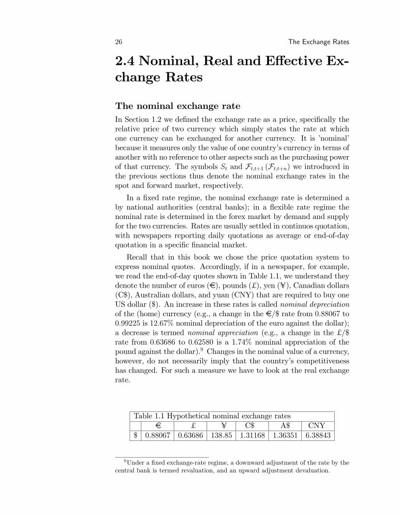
Recall that in this book we chose the price quotation system toexpress nominal quotes. Accordingly, if in a newspaper, for example,we read the end-of-day quotes shown in Table 1.1, we understand theydenote the number of euros (e), pounds (£ ), yen (U), Canadian dollars(C$), Australian dollars, and yuan (CNY) that are required to buy oneUS dollar ($). An increase in these rates is called nominal depreciationof the (home) currency (e.g., a change in the e/$ rate from 0:88067 to0:99225 is 12:67% nominal depreciation of the euro against the dollar);a decrease is termed nominal appreciation (e.g., a change in the £ /$rate from 0:63686 to 0:62580 is a 1:74% nominal appreciation of thepound against the dollar).9 Changes in the nominal value of a currency,however, do not necessarily imply that the country�s competitivenesshas changed. For such a measure we have to look at the real exchangerate.

Table 1.1 Hypothetical nominal exchange ratese £ U C$ A$ CNY

$ 0:88067 0:63686 138:85 1:31168 1:36351 6:38843

9Under a �xed exchange-rate regime, a downward adjustment of the rate by thecentral bank is termed revaluation, and an upward adjustment devaluation.


The real exchange rateThe real exchange rate, like the nominal one, is a relative price ob-tained from the nominal exchange rate adjusted for the relative pricelevels between the home and the foreign country. It gives a measureof competitiveness, which tells how much the goods and services inthe domestic country can be exchanged for the goods and services in aforeign country. Formally, letting P , P � and S denote the price levelin the home country, the price level in the foreign country, and the(spot) nominal exchange rate, respectively, we can write the date t realexchange rate, Qt, as

Qt =StP

�t

Pt: (1.6)

A rise in Q is called real depreciation, and can be the result of a nom-inal depreciation (a rise in S), a rise in the relative prices (P �t =Pt), orboth. It signals a real depreciation of the home currency, which meansthat foreign goods are now more expensive for domestic residents (thedomestic price of a bundle of foreign goods has risen). For example,if in a given period the yen/dollar nominal rate changes from 120; 70to 132; 77 (a 10% nominal depreciation) while the relative prices re-main unchanged, say to (P �t =Pt) = 100=100 = 1, then the U/$ realrate

�QU=$

�undergoes a real depreciation of 10%, thus signaling that a

basket of US goods costs now relatively more for JP residents as theyhave to pay U132; 77 to purchase the original bundle of US goods ofU120; 70. The same result obtains if we let the nominal rate be un-changed and the US price index rise of 10% (from 100 to 110), or takeany convex combination of changes in nominal rate and relative pricesthat ends up in an upward rise of 10% (e.g., a 5% increase in both Stand P �t =Pt).A fall in Q is termed a real appreciation, and can be the result

of a nominal appreciation, a decrease in the relative prices, or both.It signals a real appreciation of the home currency, and means thatforeign goods are now less expensive for domestic residents. A simpleexample follows by simply reversing the changes applied in the abovereal depreciation case.It should now be point out that in the literature there are a number

of alternative ways of measuring the relative prices and hence the realexchange rates. A useful though not exhaustive list is given below.10

� If all goods are postulated to be traded internationally, P =PX , that is, the domestic price index equals the price of exports�PX�, and similarly P � = PM, where PM is the price of imports.

10More detailed and excellent surveys can be found, e.g., in Maciejewski (1983),Edwards (1989b), Hinkle and Montiel (1999), Harberger (2001, 2004), Chin (2006).


Substitution into (1.6) yields

Qt =StP

Mt

PXt; (1.6a)

which relates the real exchange rate to the inverse of terms oftrade (the ratio between the exports and imports price PX=PM).11

Equation (1.6a) tells the amount of exports that are required toobtain one unit of import. As a result, an increase in Q signalsa deterioration in the terms of trade, as it means that a grateramount of exports are required to obtain one unit of imports,whereas a fall denotes an improvement in PX=PM.

� If the price index is supposed to be a geometric average of socalled traded- and nontraded-goods (i.e., goods that are tradedor not internationally), both the domestic and foreign price levelcan be written as

Pt =�PNt� �

P Tt�1�

P �t =�P �Nt

�� P �Tt

�1��;

where the superscripts N and T stand for non-tradable and trad-able goods, and and � are the shares of non-tradables in thegeneral price index for the domestic and foreign economy, respec-tively.12 Substituting into (1.6) yields

Qt =

StP

�Tt

P Tt

!264�P �

N

t =P �Tt

��P

N

t =PTt

� 375 ;

or, letting for simplicity � = 0, i.e., assuming that the foreigneconomy produce only tradable goods (so that SP �T = P T , ifPPP holds; (see, Chapter, Sect. ),

Qt =

�P TtPNt

� : (1.6b)

11Things do not change, however, if we recognize that exports and imports areparts of domestic and foreign output.12Generally, the key element to consider when looking at the tradable and non-

tradable classi�cation is where the price for the good (or service) is determined.If it takes place in the world market, the good should be considered tradable.If the price determination takes place in the local market, the good should beconsidered non-tradable. Water supply, all public services, hotel accommodation,real estate, construction, local transportation are examples of nontradable goods;cars, electronics, clothing, machinery and equipment, oil and raw materials areexample of traded goods.


Equation (1.6b) de�nes Q as the internal relative price incen-tive for producing (or consuming) tradable goods as opposed tonon-tradable goods, which makes it an indicator of incentivesto allocate resources in the home country. As a consequence, andecrease (increase) in Q indicates that in the home country incen-tives to allocate resources in the less competitive, non-tradablesector have risen (declined).

If cost competitiveness is a focus of attention, another alternativeis the relative unit labour costs between the domestic and foreign econ-omy. In this case, the real exchange rate is de�ned as

Qt =StW�

t

Wt

; (1.6c)

where W and W� are unit labour costs, respectively.13 An rise (de-crease) in foreign relative to domestic unit labour costs (W�

t =Wt)meansan improvement (deterioration) in the external competitiveness of thehome country, which causes the real exchange rate to appreciate (de-preciate) and the real value of the currency to depreciate (appreciate).This is because a rise in (W�

t =Wt) is re�ected in a rise of relative price(P �=P ) and hence of Q as shown in Equation (1.6).

The e¤ective exchange rateSo far, the discussion of the (nominal and real) exchange rate has in-volved only two countries (currencies). This is a convenient simpli�-cation in that it allows one to de�ne the theoretical construct whileabstracting from third-country e¤ects. Nevertheless, in the real worlda country typically trade not with a single country but with a numberof countries, so it is crucial to have a measure of the overall exter-nal value of a country�s currency relative to all other currencies beingtraded. This is what the e¤ective exchange rate aims to. It is usu-ally presented as an index number with a base of 100, so as to showan appreciation when it increases (index above 100) and a depreciationwhen it decreases (index below 100). E¤ective exchange rates index arecomputed and published by international �nancial institutions such asthe International Monetary Fund (IMF), the World Bank (WB), Bankof International Settlements (BIS), by central banks and private insti-tutions.Like the two-country case, the are two di¤erent measures: the nom-

inal e¤ective exchange rate and the real e¤ective exchange rate. Thenominal e¤ective exchange rate (NEER) measures the average value of

13Unit labor costs are routinely computed as ratio between nominal wage rateand labour productivity.


a country�s exchange rate against all other trading partners. Formally,it is computed as

Si;NEERt =

�1

S1it

�!1��1

S2it

�!2� � � � �

�1

Snit

�!n;

or

Si;NEERt =nY

j=1;j 6=i

�1

Sjit

�!j;

nXj=1;j 6=i

!j = 1; (1.7)

where Si;NEERt is the nominal e¤ective exchange rate of currency/countryi, Sjit the nominal exchange rate of currency/country i relative to cur-rency/country j, expressed in direct quotation form (the price of for-eign currency in terms of domestic currency), !j the weight assigned tocurrency j in the computation of the index, usually based on bilateraltrade volumes (the sum of exports and imports, expressed as a pro-portion of total exports and imports), and

Ya symbol denoting the

product of elements�1=Sjit

�!j . Equation (1.7) shows that the NEER iscomputed as a geometrically weighted average (or convex combination)of nominal bilateral exchange rates, where the sum of weights is equalto one by de�nition. Observe, that in order to make changes in theSi;NEER index consistent with changes (appreciation or depreciation)in the nominal bilateral exchange rates Sji we used the inverse of directquotation (1=Sji) and not simply the direct quotation (Sji), as it wouldhave been the case had we used the volume quotation system.14

The real e¤ective exchange rate (REER) is an overall measures of acountry�s competitiveness against the other trading partners. It can becomputed as in (1.7) using real rather than nominal bilateral exchangerates. Formally, we have

Qi;REERt =

nYj=1;j 6=i

�1

Qjit

�!j;

nXj=1;j 6=i

!j = 1; (1.8)

which computes the real e¤ective exchange rate of country i�Qi;REER

�as a geometrically weighted average of real bilateral exchange rates Qji.

14A linearized version of (1.7), often found in the literature, is

si;NEERt = ��!1s

1it + � � �+ !nsnit

�= �

nXj=1;j 6=i

!jsjit :

It can be obtained from (1.7) by taking logs of both sides, and denoting log variableswith lower-case letter.

Chapter 3

Currency Derivatives and Op-tions Markets

3.1 Introduction

We learned from previous Sections that the forex market is a very largemarket with many di¤erent features, advantages and risks. We alsolearned that forex investors may trade in futures as well as spot mar-kets. Yet, when looking at the forward markets we hear of a numberof �nancial instruments that can be used by agents for speculation, ar-bitrage and hedging activities. These �nancial instruments are knownas currency derivatives and they have seen an enormous growth since1970. This Section gives an overview to the main types of derivativeinstruments used in the forex market: futures, options and swaps.Financial derivatives are traded either on organized derivatives ex-

changes (ODE) markets, such as the Chicago Board Options Exchange(CBOE), the Japan Exchange Group (JPX), the New York Stock Ex-change London international �nancial futures exchange (NYSE Li¤e),etc., or in Over-The-Counter (OTC) markets. The di¤erences betweenthese two competing market segments are not only from where thetrading takes place but also how. In the exchange-traded segment,derivatives contracts are highly standardized with speci�c delivery orsettlement terms. Trades and prices are publicly reported and clearedin a clearing house, making risks and market trends transparent to allmarket participants and regulators. In addition, the clearing house is

31

32 Currency Derivatives and Options Markets

obliged to honour the trade if the seller defaults and the solvency ofthe clearing house is protected by marking all positions to market dailythrough a system of margins.By contrast, in the OTC segment derivatives contracts are traded

bilaterally and arranged on a tailor-made basis. All contract terms re-garding the underling asset, contract size, price, maturity and otherfeatures are negotiable between the two parties. Transactions are set-tled by telephone or other communication means, and prices are notreported publicly.These di¤erent features of ODE and OTC derivatives markets mean

that they can both complement and compete with each other. Forexample, OTC derivatives can rely on high liquid and price transparentODE markets to dynamically hedge their market risk. Conversely,ODE derivatives can face competitive pressure from more �exible OTCmarkets on price and services.1

3.2 Futures

A currency future, or FX future is a futures contract to exchange onecurrency for another at a given date in the future at a price (exchangerate) that is �xed on the purchase date.

3.3 Options

A currency option, or FX option is a contract that grants the holder theright, but not the obligation, to buy or sell a currency at a pre-agreedprice (exchange rate) for a speci�ed time period.

3.4 Swaps

A currency swap, or FX swap is a simultaneous purchase and sale ofidentical amounts of one currency for another with two di¤erent valuedates (normally spot to forward).To be completed.

1See, e.g., Nystedt (2004), Switzera and Fanb (2008), Deutsche Börse Group(2008), Prabha, Savard and Wickramarachi (2014).

Part II

The Balance of PaymentsAccounts

33

Chapter 4

Balance-of-Payments and In-ternational Investment Posi-tion

4.1 Introduction

In this chapter we shall look at the balance-of-payments (BP) accountand International Investment Position (IIP) which are among the ma-jor economic indicators for policymakers and private agents in an openeconomy. The main reason for such a prominent role is that they givesan o¢ cial account of all transactions and positions between an econ-omy and the rest of world, so signaling the performance of a countryin international markets including trading and capital �ows with othernations, exchange rate policy, reserves management, and external vul-nerability.The major purpose of this chapter is to provide a comprehensive

summary of what data are included in these accounts, how they arecompiled and classi�ed and of possible economic interpretations of thestatistics. We discuss the general accounting principles guiding thecompilation of the basic structure of a BP account and of di¤erentcomponents that are included. We also discuss the meaning of surplus,de�cit and equilibrium in the main accounts, and how the BP andIIP accounts are related. We �nally look at how balance of paymentsaccounts and data on the international investment position can be in-

35

36 Balance-of-Payments and International Investment Position

terpreted within the framework of the national income accounts, so�tting the main macroeconomic variables and accounting relations inan open economy context.

4.2 System Structure and Account-ing Principles

The balance of payments is a statistical statement that systematicallysummarizes all the economic and �nancial transactions of a countrywith the rest of the world over a speci�c time period. These transac-tions involve interactions between residents and nonresidents, or foreignresidents of a country, and include payments for the country�s exportsand imports of goods, services, �nancial capital, and �nancial trans-fers.1 The international investment position, on the other hand, is astatistical statement that shows the value and composition of the stockof an economy�s �nancial assets and liabilities with the rest of the world.Therefore, the balance of payments records the �ows of payments ina given time period, whereas the international investment position isconcerned with �nancial stocks at given point in time. Figures on theseaccounts are normally reported in the domestic currency of the compil-ing country and calculated over a month, a quarter or more commonlyover a year.

4.2.1 Accounting Principles

The accounting principles behind balance-of-payments statistics derivefrom the double-entry bookkeeping system, which means that every

1The notions of �resident�and �nonresident�are however problematic, as citizen-ship and residency do not necessarily coincide from the viewpoint of BP statistics.The International Monetary Fund (IMF) in its Manual provides a set of rules tosolve doubtful cases. The general criterion for determining residence builds aroundthe concept of center of predominant economic interest de�ned as "the economicterritory to which each entity is most closely connected" (see, IMF, 2009, p. 89).For example, all members of the same household have the same residence as thehousehold itself, even though they may cross borders to work or otherwise spendperiods of time abroad; similarly, corporations and other institutions have the res-idence in the economy in which they are legally constituted and registered. Bycontrast, international organization such as the International Monetary Fund, theWorld Bank, the United Nations, etc. are regarded as foreign resident even thoughthey may be located in the compiling country.

Balance-of-Payments and International Investment Position 37

recorded transaction is represented by two entries with equal valuesbut opposite signs, a debit (-) and a credit (+). More speci�cally,under the conventions of the system a compiling economy records:

� credit entries for all transactions involving exports of goods andservices, income receivable, and reduction in assets or increase inliabilities;

� debt entries for all transactions involving imports of goods andservices, income payable, and increase in assets or reduction inliabilities.

Thus, a schematic representation is as follows:

Exports of goods and services Credit (+)Imports of goods and services Debt (�)Increase in liabilities Credit (+)Increase in assets Debt (�)Decrease in assets Credit (+)Decrease in liabilities Debt (�).

A key point about the double-entry bookkeeping is that in anaccounting sense the balance of payments is always in balance. This isbecause the sum of all credits should be equal to the sum of all debits,and the overall total should equal zero. To understand how this workslet us take a couple of simple examples.Suppose that Italy exports e10 billion worth of goods to the United

States and that the US importers pay from euro accounts that arekept in Italian banks. Under the double-entry system, the value ofexports will be represented by a credit entry in the Italy�s balance ofpayments and the �nancial asset acquired (bank draft or any othercredit instrument) by an o¤set debit entry. Suppose, on the otherhand, that Italian residents buy e5 billion worth of US securities andthat the US sellers put the e5 billion they receive into Italian bankaccounts. In this case, the increase in foreign assets is recorded as adebt entry and the payment as an o¤setting credit entry. These BPrecording rules are set out in Table 1.2.

Table 1.2 Examples of Balance of Payments RecordingCredit Debt

Exports of goods 10Bank deposits (increase in �nancial assets) -10Increase in foreign assets -5Bank deposits (reduction in �nancial assets) 5


Nonetheless, the accounts never add to zero in practice, either be-cause data estimates are often derived from di¤erent sources and maybe incomplete, inconsistent and subject to inevitable measurement er-rors or because timing and valuation e¤ects along with a variety ofother factors tend to cause imbalances in the information recorded. Asa consequence, a separate entry, equal to the amount of the resultingimbalances with the sign reversed and labelled net errors and omis-sions, is included to balance the overall account (see next Section).

From a foreign exchange perspective, however, a key point to emergefrom the above examples and, more generally, from a county�s balance-of-payments statistics is that any transaction that is recorded as acredit entry represents a demand for its home currency (or a supplyof foreign currency) in the foreign exchange market. Conversely, anytransaction that is recorded as a debt entry represents a supply ofits home currency (or a demand for foreign currency) in the foreignmarket. Therefore, credit entries imply demands for a country�s homecurrency and result from exports of goods and services, income receiv-able, and sell of �nancial and real assets to foreign residents. Similarly,debt entries imply supplies of a country�s home currency and resultfrom imports of goods and services, income payable, and purchase of�nancial and real estate to foreigners. Since the BP statistics record allthe economic transactions of an economy with the rest of the world, itfollows that they also include a list of all potential factors that lie be-hind the demand and supply curve for a currency. This is what makesthe balance-of payments account such a useful and powerful frameworkfor understanding the factors that in�uence the supply and demand ofa currency and hence the exchange rate.

The full meaning of this statement will become clear as we considerthe basic structure and classi�cation system of BP and IIP statistics.

4.2.2 Standard Components

According to the Sixth edition (2009) of the IMF�s Balance of Paymentsand International Investment Position Manual (BPM6), the standardcomponents in the BP framework are comprised of two main sections:the current account and the capital and �nancial account. The currentaccount includes all transactions that pertain to goods and services, in-come, and current transfers. The capital and �nancial account pertainsto capital transfers, transactions in nonproduced non�nancial assets,and �nancial assets and liabilities. Examples of balance-of-payments


for Italy and the euro area are in Table 1.3.

Table 1.3 Summary Balance of Payments, 1st Quarter, 2015(EUR billions)

Italy Euro area (EU19)y

Credits Debits Net Credits Debts Net1) Current Account 131.9 131.0 0.9 833.3 778.8 54.5Goods 96.0 86.6 9.4 496.1 428.9 67.2Services 18.2 20.5 -2,4 166.9 157.1 9.8Primary incomes 14.7 13,8 1.0 146.9 118.9 28.0Secondary incomes 3.0 10.1 -7.1 23.4 73.9 -50.52) Capital Account 0.6 0.9 -0.3 8.4 4.5 3.93) Net Lending/Bor-rowing to/from ROWz 0.6 58.4(1+2)4) Financial Account 4.8 11.1 -6.3 504.8 513.7 -8.8Direct investment 8.6 3.8 4.8 159.7 74.7 85.0Portfolio investment 59.9 67.8 -7.9 129.0 260.2 -131.2Financial derivatives -1.7 27.3Other investment 3.4 4.5 -1,1 182.8 178.7 4.1Reserve assets -0.4 6.0Errors and omissions -6.9 -67.2yEU 19: Austria, Belgium, Cyprus, Estonia, Finland, France, Germany,Greece, Ireland, Italy, Latvia, Lithuania, Luxembourg, Malta, the Ne-therlands, Portugal, Slovakia, Slovenia, and Spain.zROW: Rest of the World.Source: BOI (2015), ECB (2015).

Current AccountThe current account includes all transactions that pertain to goods,services, and primary and secondary incomes (or income and currenttransfers).

� Goods:

comprises general merchandise (goods that residents export to, orimport from, nonresidents), goods for processing (exports or importsof goods crossing the frontier for processing abroad and subsequentre-import or export of the goods), repairs on goods (repair activity ongoods provided to or received from nonresidents on ships, aircraft, etc.),goods procured in ports by carriers (goods such as fuels, provisions,stores, and supplies that resident/nonresident carriers (air, shipping,etc.) procure abroad or in the compiling economy), and nonmonetary


gold (exports and imports of all gold not held as reserve assets by theauthorities).Goods are recorded according to the fob (free on board) de�nition,

both for exports and for imports, so that they are valued at the frontierof the exporting country. The receipts for exports are recorded as cred-its, the payments for imports are recorded as debits, and the di¤erence(Net in Tab.1.3) is referred as goods balance. When the balance is insurplus this means that the revenues for exports are greater than theoutlays for imports (credits>debits) and the di¤erence appears witha positive or no sign in the balance of payments. Conversely, whenthe balance is in de�cits (credits<debits) the di¤erence appear with anegative sign.

� Services:

comprises transportation (services such as freight, passenger trans-portation by all modes of transportation and other distributive andauxiliary services that are performed by residents for nonresidents andvice versa), travel (goods and services acquired by nonresident travel-ers for business and personal purposes during their visits of less thanone year in a country), other services (service transactions with non-residents not covered under transportation or travel, such as communi-cation services, construction services, insurance or �nancial services).As for goods, credits denote export revenues, debits import pay-

ments, and the di¤erence (Net) the surplus (+) or de�cit (-) in thebalance of service. The sum of balance on goods and services is oftenreferred as trade balance.

� Primary income:

shows income �ows between residents and non residents in returnfor providing temporary use to another entity of labor, �nancial re-sources, or nonproduced non�nancial assets. It includes compensationof employees (wages, salaries and other bene�ts, including social contri-butions and private insurance policies or pension funds), investment in-come (dividends, withdrawals from income of quasi-corporations, rein-vested earnings, interest, and investment income attributable to pol-icyholders in insurance, standardized guarantees and pension funds),and other primary income (rents, taxes and subsidies on products andproduction).

� Secondary income:

shows current transfers that are not transfers of capital betweenresidents and nonresidents without anything of economic value being


supplied as a direct return. It comprises government transfers (currenttaxes on income and wealth, social contributions and social bene�ts,current international cooperation, miscellaneous current transfers, etc.)and transfers of other sectors (workers�remittances, insurance premi-ums, claims on non-life insurance, and other transfers such as �nes andpenalties, gifts and donations, etc.).As for goods and services, in�ows from nonresidents are considered

as credit entries, out�ows as debit entries, and the di¤erence as thesurplus or de�cit in the income balance.Computation of the subtotal up to the secondary income account

yields the current account of the balance of payments, which shows theamount of credits and of debits in the goods, services and income ac-counts (see, Tab 1.3). When the sum of exports and income receivableexceeds the sum of imports and income payable the current accountbalance (Net) is in surplus; conversely, when total imports and incomepayable exceeds exports and income receivable it is in de�cit. Table1.3 shows that in 1st Quarter of 2015 the current account balances forItaly and the euro area were in surplus by e 0.9 billion and by e 54.5billion, respectively.

Capital AccountThe capital account shows credit and debit entries for nonproducednon�nancial assets and capital transfers between residents and nonres-idents.

� Nonproduced, non�nancial assets:

refers to transfers of ownership between residents and nonresidentsof natural resources (land, mineral rights, forestry rights, water, �shingrights, air space, and electromagnetic spectrum); licenses, leasing con-tracts and other contracts (intangibles such as marketable operatingleases, permissions to use natural resources not recorded as outrightownership of those resources or to undertake certain activities includ-ing some government permits, and entitlements to purchase a goodor service on an exclusive basis); and marketing assets (brand names,trademarks, logos, etc.) and goodwill.

� Capital transfers:

refers to transfers of ownership of �xed assets; transfers of fundslinked to the acquisition or disposal of �xed assets and the forgivenessof debts. Capital transfers are classi�ed into two sectorial components:general government (capital taxes, debt forgiveness, investment grantsand the other capital transfers) and other sectors (migrants�transfers,debt forgiveness and other transfers).


Net Lending/BorrowingThe sum of the balances on the current and capital accounts showsthe net lending (surplus) or net borrowing (de�cit) by the compilingcountry with the rest of the world. The reason the balance item netlending/borrowing is reported is that it re�ects the amount of �nancialassets that are available for lending or needed for borrowing to �nanceall transactions with non residents. It is conceptually equal to the netbalance of the �nancial account, although in practice the equivalenceis hardly got.

Financial AccountThe �nancial account records all transactions in external �nancial as-sets and liabilities. It is structured around �ve accounts, di¤erentiatedby the type of �nancial assets/liabilities involved in the transaction.

� Direct investment:

involves cross-border investments associated with residents in onecountry having control or signi�cant in�uence over the management of�rms resident in another country, and tends to be associated with last-ing relationships. Direct or indirect possession of 10 per cent or moreof the voting rights is proof of such a relationship. Direct investmentis classi�ed according to the instrument involved and comprises shares,other equity, reinvested earnings and debt instruments.

� Portfolio investment:

covers transactions between residents and non-residents involvingdebt and equity securities not included under direct investment. Portfo-lio investment is classi�ed according to shares, investment fund shares,debt securities (short or long-term) and divided by resident sector andcounterparty sector.

� Financial derivatives:

covers �nancial instruments linked to other �nancial instrumentsthrough which speci�c �nancial risks can be traded in �nancial mar-kets. Transactions and position recorded under this item are those inoptions, futures, swaps, forward foreign exchange contracts and creditderivatives.

� Other investment:


involves positions and transactions other than those included in di-rect investment, portfolio investment, �nancial derivatives and reserveassets. It comprises: equity other than securities; currency and de-posits; loans, insurance, pension schemes and standardized guarantees;trade credit and advances; other accounts receivable/payable; and SDRallocations (SDR holdings are included in reserve assets).

� O¢ cial reserves (reserve assets):

comprises external assets that are readily available to and controlledby monetary authorities for meeting balance of payments �nancingneeds, for intervention in exchange markets to a¤ect the currency ex-change rate, and for other related purposes (such as maintaining con�-dence in the currency and the economy, and serving as a basis for for-eign borrowing). They include monetary gold, special drawing rights(SDR) holdings, reserve position in the IMF, foreign currency and de-posits, securities (including debt and equity securities), �nancial deriv-atives, and other claims (loans and other �nancial instruments)

Errors and OmissionsThis item is the result of errors and omissions in the compilation ofbalance-of-payments statements. It is derived residually from the netbalance of the �nancial account minus the same item derived from thesum of the current and capital accounts, or net lending/net borrowing.Table 1.3, for example, shows that net lending/net borrowing measuredfrom the current and capital accounts for Italy is 0.6, while the netbalance measured from the �nancial account is -6.3; then, errors andomissions is -6.9.Because the net lending or net borrowing derived from the current

and capital account should in principle be equal to the overall balanceon the �nancial account - for a surplus of credits over debits in thecurrent and capital accounts there is a balancing net acquisition of�nancial assets or reduction of liabilities which is shown in the �nancialaccount -, it follows that a positive value of (net) errors and omissionssignals that credit entries have been understated or debit entries havebeen overstated, and vice versa in case of a negative value.

International Investment PositionClosely related to the �ow-oriented balance of payments framework isthe stock-oriented international investment position. It is a statisticalstatement that shows at a point in time the value and compositionof (i) �nancial assets of residents of an economy that are claims onnonresidents and gold bullion held as reserve assets, and (ii) liabilities


of residents of an economy to nonresidents. The di¤erence betweenthe two sides of the balance sheet measures the economy�s net IIP,which may be positive or negative. As shown in Table 1.4, the IIPpresentation format comprises the same items as the �nancial account,namely, direct investment, portfolio investment, �nancial derivatives,other investment, and o¢ cial reserves. Table 1.4 signals a net IIP forItaly and the euro area at the end of 2015-Q1 of e -478.3 and -1,294.5billions, respectively.The balance of payments and international investment position can

be reconciled, as the change in the stock of external �nancial assets andliabilities in a period is attributable to �nancial �ows (transactionson the �nancial account of the balance of payments) and valuationadjustments (referring to the changes between the start and the endof the period in exchange rates and the prices of underlying assets andany other adjustments). The next section discusses in more detail theissue.

Table 1.4 International Investment Position, 1st Quarter, 2015(end-of-period stocks in billions of euros)

Italy Euro area (EU19)Assets Liabilities Net Assets Liabilities Net

Direct investment 564.9 418.1 146.8 8,204.4 6,331.7 1,872.7Portfolio investment 1,073.2 1,481.4 -408.2 7,270.9 10,995.3 -3,724.4Financial derivatives 131.3 200.7 -69.4 -21.0 -21.0Other investment 466.6 744.1 -277.5 5,029.9 5,054.9 -25.0Reserve assets 130.0 130.0 603.1 603.1

Total net position 2,366.0 2844.3 -478.3 21,087.3 22,381.9 -1294.6Source: BOI (2015), ECB (2015).

Chapter 5

Some Linkages between BP,IIP, and National Accounts

5.1 Introduction

This section discusses the major links among the balance of paymentsaccounts, international investment position and the broad system ofnational accounts. The goal is to: (i) draw from the �ows, stocks, andother changes a¤ecting the level of assets and liabilities over a giventime period some basic relations among the main macroeconomic vari-ables in an open economy; (ii) provide an introduction to the factorsin�uencing international transactions and positions, and the extent towhich such factors are sustainable; (iii) consider some of the implica-tions of balance of payments �nancing and adjustments for economicpolicy.It should be pointed out, however, that in this Section the link-

ages between an economy�s domestic sectors and the rest of world areexpressed as simple accounting identities from which no causal rela-tion should be inferred. Though useful in describing those relation-ships, identities provide only a starting point for an analysis of theinteraction among the main macroeconomic variables in an economicsystem. To draw casual relations, identities must be supplemented byspeci�c hypotheses about the factors that determine the behavior ofprivate agents and government sectors of the whole system. A deeperunderstanding of this approach will turn up as we discuss theoretical

45

46 Some Linkages between BP, IIP, and National Accounts

modelling in international �nance in the next chapters.

5.2 Balance of Payments and Na-tional Accounts

In an open economy, the following two basic identities are commonlyused to describes the balance between output, or aggregate supply,and aggregate expenditure, or use, of a country. The �rst de�nes grossdomestic product (GDP ) as

GDP � C + I +G+X �M; (5.1a)

where C =domestic consumption, I =domestic (private) investment,G =government expenditure,X =exports of goods and services,M =importsof goods and services, and � a binary relation denoting equivalence,used to di¤erentiate between identities, or accounting relations, andbehavioral, or theoretical equations. Identity (5.1a) is the familiar ex-penditure approach to GDP .The second de�nes gross national product (GNP ) as

GNP � GDP +NY B; (5.1b)

where NY B =net income balance on primary and secondary incomefrom abroad. The relation in (5.1b) is the income approach to GDP .Substitution of (5.1a) in (5.1b) implies

Y � C + I +G+X �M+NY B; (5.2)

where Y is GNP .If we now deduct taxes (T ) from both sides of (5.2), we obtain

Yd � C + I +G� T +X �M+NY B; (5.3)

where Yd � Y � T denotes disposable income.Balance-of-payments statistics shows that the current account bal-

ance (CA) isCA � X �M+NY B; (5.4)

that is, the sum of balance on goods and services (X �M) and balanceon income accounts (NY B). Thus, (5.3) can be rewritten as

Yd � C + I +G� T + CA: (5.5)

Some Linkages between BP, IIP, and National Accounts 47

As de�ned in the system of national accounts:

Sp � Yd � C (5.6a)

Sg � T �G (5.6b)

S � Sp + Sg; (5.6c)

where Sp = private saving, Sg = public, or government saving, andS =national, or aggregate saving. Use of (5.6a)-(5.6c) in identity (5.5)then yields

CA � S � I � Sp + Sg � I � (Sp � I) + (T �G) : (5.7)

This identity points out that the current account re�ects the gapbetween saving and investment of an economy, with a current accountsurplus indicating that national saving exceeds investment, or that pri-vate savings exceeds (private) investment and/or government budget isin surplus, and vice versa with a current account de�cit. It is worthyto restate, however, that (5.7) is merely an identity that tells nothingabout causation. Thus, it might be either that the current accountde�cit is the result of a shortage in private saving and/or a governmentbudget de�cits, or that the lack of national saving is due to the cur-rent account de�cit. Put more simply, what identity (5.7) suggests isthat any change in an economy�s current account balance (e.g., a largersurplus or smaller de�cit) must necessarily be matched by a change insaving relative to investment (e.g., an increase in domestic saving rel-ative to investment). This highlights the relevance of understandingand assessing the e¤ects on saving and investment of policy measures(e.g. changes in exchange rates, tari¤s, etc.) designed to change thecurrent account balance.An alternative way of expressing the link between the external and

internal sectors of an economy shown in identity (5.7) is as follows. LetA � C + I +G denote domestic absorption or expenditure and rewrite(5.2) as

Y � A+ CA:

It follows thatCA � Y � A; (5.8)

which states that the current account equals the di¤erence betweennational income and absorption. The implication of this relationshipis the same as that noted above and tells nothing about causality. Itsimply states that any changes in a country�s current account (e.g., alarger surplus) require changes in domestic absorption relative to na-tional income (i.e., a contraction in A, or an increase in Y ). Hence, itwould be inappropriate to use the identity (5.8) to analyze the impact


of changes in Y or A on the current account balance without under-standing the reaction of both private agents and the government tosuch changes.As shown in the previous chapter and in Tab.1.3, the balance of pay-

ments statistics include not only the current account (i.e., the exchangeof goods and services, and the receipt and payment of income and trans-fers) but also the capital and �nancial account (i.e., the �ow of �nancialtransactions involving changes in �nancial claims on, and liabilities to,the rest of the world). Also, the basic principle of double-entry book-keeping implies that the sum of all international transactions� current,capital, and �nancial� is in principle equal to zero, though they maynot balance in practice owing to errors or omissions. Assuming forsimplicity that there are no recording errors or omissions, this balancebetween the �nancial account and the current and capital account canbe expressed as

NLB � CA+KA � NFA; (5.9)

or, alternatively, as

CA� (NKFA+�FR) � 0; (5.10)

where NLB = net lending/net borrowing, KA = the capital accountbalance, NFA = net �nancial account, �FR = change in reserveassets, and NKFA � (NFA+KA)��FR =net capital and �nancialaccount (i.e., all capital and �nancial transactions excluding reserveassets).The identity in (5.9) simply formalize the idea that in standard

presentations of BP statistics net lending/net borrowing from the sumof the current account and capital account balances is conceptuallyequal to net lending/net borrowing from the �nancial account. Theidentity in (5.10) shows that the sum of all current, capital and �nancialaccount items, including reserve assets, is equal to zero. This means

CA � NKFA+�FR; (5.11)

which states that that the net provision of resources to or from therest of the world, as measured by the current account balance, must�by de�nition� necessarily be matched by a change in net capital and�nancial account balance plus foreign reserve assets. Thus, a surplus(de�cit) in the current account is re�ected in an increase (decrease) innet claims held by the private sector or government on nonresidents(NKFA) or an increase (decline) in o¢ cial reserve assets (�FR), orboth. From this perspective, the identity in (5.11) can be thought ofas describing the budget constraint for the whole economy.Because the above balance-of-payments accounting framework hold

irrespective of the exchange rate regime adopted by a country, it is


useful to consider the implications of the fundamental relationship de-scribed in (5.11) separately for �xed, �exible and managed exchangerates.

Fixed ratesUnder a �xed or pegged exchange rate system, the country�s mone-tary authorities intervene in the forex market to prevent exchange ratechanges using its o¢ cial reserves. Accordingly, transactions in reserveassets will be determined by the net demand or supply of foreign ex-change at that exchange rate, namely

�FR � CA�NKFA:

This identity tells us that when exchange rate are �xed the change ino¢ cial reserves equals the combined surplus/de�cit di¤erence in thecurrent and capital account. Consequently, when CA � NKFA > 0(a BP surplus) the net excess demand of the country�s currency in theforex market will force the monetary authority to supply an amountof its currency equal to the excess demand, thereby purchasing foreigncurrency and creating �FR > 0. Similarly, when CA � NKFA < 0(a BP de�cit) the monetary authority will buy whatever excess supplyof its currency appear in the foreign market at the �xed rate, therebyselling foreign reserves and creating �FR < 0.In short, under a �xed-rate system the monetary authorities had to

accommodate any change in the demand of their currencies if they wereto prevent their exchange rates from changing. Therefore, �FR hadto be equal to the combined balance on current and capital accountCA�NKFA.

Flexible ratesUnder a pure �oating (truly �exible) exchange rate arrangement, therecannot be any change in o¢ cial reserves because central banks do notintervene in the forex market to a¤ect the valuation of the exchangerate. Accordingly, �FR = 0 and

CA � NKFA:

This identity shows that with �exible exchange rates, the (correctlymeasured) current account balance is exactly equal to the (correctlymeasured) capital and �nancial account balance, so that BP � CA�NKFA = 0. What happens under a pure �oat regime is that any im-balance in a country�s balance of payments (BP 6= 0) will automaticallyalter the exchange rate in the direction necessary to obtain BP = 0.


Therefore, a BP surplus (CA�NKFA > 0) should lead the exchangerate to appreciate, thereby making domestic goods and assets moreexpensive on international markets and applying downward pressureson the current account (and balance of payments) surplus. Similarly, aBP de�cit should lead the exchange rate to depreciate, thereby causingimprovements in CA and BP .

Managed ratesIn the intermediate case of a managed �oat, purchases and sales ofreserve assets by central banks are typically undertaken to achieve adesired exchange rate path for the domestic currency in terms of oneor more foreign currencies. Accordingly, a BP imbalance should leadto changes in reserves assets, the exchange rate, or both so as to getCA� (NKFA+�FR) = 0.

Balance of payments �nancingThe interrelationship between the current account and the capital and�nancial account can be seen more clearly by using the identities in(2.7) and (2.8), which state that the current account equals the di¤er-ence between total domestic saving and investment or, alternatively,the gap between income and domestic expenditure. Hence, (2.11) wecan be rewritten as

CA � S � I � Y � A � NKFA+�FR: (5.12)

This identity describes the �ows of resources and �nancial assets overtime. It states that any gap between saving and investment or do-mestic income and expenditure, which is re�ected in a current accountimbalance, is matched by a change in private assets or o¢ cial assets,or both. Thus, to the extent that domestic capital accumulation (I)or domestic absorption (A) is not matched by an increase in domes-tic saving (S) or domestic income (Y ) there will be a current accountde�cit, which must be �nanced by a reduction in net foreign assets heldby the private sector or government (NKFA) or a reduction in o¢ cialreserve assets (�FR), or both. Obviously, the opposite comes aboutin the excess of saving case or current account surplus.Nevertheless, if the gap between income and expenditure revealed

not to be temporary or reversible, and hence persist over an extendedperiod of time, then concerns about the country�s external paymentsposition are likely to materialize eventually, leading to abrupt andpainful adjustments up to the possibility of a balance of paymentscrisis. This is because with CA < 0, for example, a country is �nanc-ing the excess of consumption and investment over national income by


using private and/or o¢ cial assets or by borrowing abroad. This is notsustainable in the long run, because (i) the stock of reserve assets islimited and bound to be exhausted in a �nite time, and (ii) the increasein liabilities (borrowing abroad) and/or the decline in foreign assets re-duce the net �ows of the income account. As a consequence, the currentaccount de�cits increases further and this can lead to a destabilizingsituation in which the current account balance progressively worsensunless changes in economic policies (e.g., expenditure reducing policies)or adjustments in certain variables (e.g., exchange rates) are made toarrest the deterioration and avert a balance of payments crisis.Problems may also arise when a country is facing a persistent cur-

rent account surplus. In this case, the excess of aggregate saving overdomestic investment or of income over expenditure is re�ected in a risein net foreign assets held by the private sector or a buildup of o¢ -cial reserve assets, or both. If expenditure expanding policies aimedat driving consumption toward foreign goods and away from domes-tic goods are not implemented, then important issue associated with�nancial stability and monetary policy management may arise for thedomestic economy. In particular, when the surplus causes a buildupof reserve assets, the economy�s monetary aggregates increase and acredit expansion will occur. If the credit expansion is too large andrapid so fuelling a credit boom, the economy may overheat, leadingto in�ationary pressures and/or vulnerabilities in the �nancial sectorespecially if weaknesses in �nancial sector supervision exist.

External vulnerability and IIPAs stressed in chapter 4, the international investment position accountshows the value and composition of a country�s international stock ofassets and liabilities. It is closely connected to the �ows of funds listedin the BP accounts, as the in�ows and out�ows of capital resulting frompurchasing and selling of �nancial assets are added to and subtractedfrom the stocks of outstanding foreign assets and liabilities. Also, theIIP is a subset of the national balance sheet and equals the net worth ofthe economy, which is the balancing item of the national balance sheet.This is because in the aggregate the �nancial assets and liabilities ofdomestic sectors cancel each other out and a country�s balance sheetconsists of its stock of domestic non�nancial assets plus its net IIP (thedi¤erence between external �nancial assets and liabilities).The severe and recurrent �nancial crises experienced in many emerg-

ing and developed economies in the last 3 decades of increasing �nancialintegration have brought the �nancial structure of economies - the com-position and size of the assets and liabilities on the economy�s �nancialbalance sheet - to the fore. It as been observed that capital �ows have


been increasingly volatile with global market integration. Financial�ows result to be high sensitive to market conditions, perceived policyweaknesses, and negative shocks. Capital in�ows can suddenly revertfollowing a decrease in con�dence about the sustainability of a coun-try�s �nancial position, such as a high level of short-term debt, andthis "sudden stop" in external �nancing often leads the economy toexperience a severe �nancial crisis.The modern literature on currency, banking and sovereign payments

crises includes a set of models for understanding the role of the �nancialsector in the build-up to crisis vulnerability. These models are nowcollected under the heading of "balance sheet approach" to �nancialcrises and provides a powerful analytical framework for exploring howbalance sheet weaknesses in one sector can a¤ect balance sheets in othersectors and give rise to a broader crisis. This approach focuses on somecommon types of balance sheet mismatches:

� Maturity mismatches, where a gap between short-term liabilitiesand long-term assets leaves an sector unable to honor its contrac-tual commitments if creditors decline to roll over debt.

� Currency mismatches, where foreign-currency-denominated oblig-ations and domestic-currency-denominated assets if unhedged leadsheavy losses following a change in the exchange rate.

� Capital structure problems, where a heavy reliance debt �nancingrather than equity �nancing leaves a �rm, a bank or a countryless able to withstand revenue shocks.

� Solvency risk, where assets values are lower than liabilities value.

� Dependency problems, where a country is overexposed to anothercountry and hence vulnerable to sudden changes about con�dencein �nancial sustainability.

Therefore, because IIP data provide information on the compositionof the �nancial structure of economies it also helps to signal the degreeof vulnerability of the economy to changes in external market condi-tions. This is why it is a so critical indicator of �nancial (in)stabilityof a country.

Part III

The Theory of ExchangeRates

53

Chapter 6

Some Fundamental Interna-tional Parity Conditions

In this chapter we look at two fundamental international �nancial rela-tionships known as the purchasing-power parity (PPP) condition andthe interest parity condition (IP).

6.1 The Purchasing Power Parity Prin-ciple

The purchasing-power parity (PPP) condition concerns the long-runrelationship between the exchange rates and the price level and appliesto goods and service markets. PPP is generally attributed to GustavCasell�s writings in the 1920s, although its intellectual origins date backto David Ricardo. The basic concept is that arbitrage forces will lead toequalization of goods prices internationally once the price of the goodsare measured in the same currency. As such the theory represents anapplication of the law of one price.This law simply states that in the presence of competitive interna-

tional markets and in the absence of transport costs and other barrierto trade, identical products which are sold in di¤erent markets willhave the same price when expressed in terms of a common currency.

55

56 Some Fundamental International Parity Conditions

Formally,Pi = SP

�i ; (6.1)

where Pi is the price of good i expressed in terms of home currency, Sis the nominal exchange rate expressed as the price of foreign currencyin terms of domestic currency, and P �i is the price of the same goodexpressed in foreign currency. Equation (6.1) is based upon the idea ofperfect goods arbitrage. Arbitrage in the goods markets occurs whereeconomic agents exploit price di¤erences to gain a riskless pro�t. Forexample, if a TV set costs e1000 in Italy and the identical model costs$1200 in the US, then according to (6.1) the free-arbitrage exchangerate should be e1000/$1300=e0.8333/$1. Imagine the exchange rateis instead e0.850/$1, then it would pay for a US resident to purchasea TV set in Italy because with $1176.5 he would obtain e1000 whichcould be used to purchase a TV set in Italy, thus saving $23.5 comparedto purchase in the US. Since agents will exploit this arbitrage possibilityas long as the di¤erence in price persists, an excess demand for euroand excess supply of dollars will start emerging in the forex market,leading the e to appreciate and the $ to depreciate. Such a processwill continue until the euro-dollar rate reach the level of e0.8333/$1.The proponents of PPP argue that the law of one price holds not

only for individual goods, but also for identical bundles of goods.Hence, (6.1) can be extended to the n-goods case to obtain

Pt = StP�t ; (6.2)

where P is the aggregate price index of all goods and services sold inthe domestic economy and expressed in the home currency (i.e., P =Pn

i=1 �iPi, withPn

i=1 �i = 1, and �i = wheight of Pi in the aggregateindex), and P � is the aggregate price index of the same goods andservices sold in the foreign country and expressed in terms of foreigncurrency (i.e., P � =

Pni=1 �

�iP

�i , with

Pni=1 �

�i = 1, and �

�i = wheight

of P �i in the aggregate index). Equation (6.2) is known as the absoluteversion of PPP. It states that a rise in the domestic price level relativeto the foreign price level will lead to a depreciation of the domesticcurrency against the foreign currency and vice versa, and can be easilyunderstood by rewriting (6.2) as

St =PtP �t: (6.2a)

Equation (6.2) is unlikely to hold exactly in the real world wheretransport costs, imperfect information and distorsing e¤ects of tari¤sand other form of protectionism may introduce marked deviations fromPPP, especially in the short-run. Nevertheless, proponents of PPPargue that a weaker form known as relative purchasing-power parity

Some Fundamental International Parity Conditions 57

(RPPP) can be expected to hold even in the presence of such dis-tortions. This version can be obtained from (6.2) by taking logs anddi¤erentiating with respect to time. Hence,

�pt =

�st +

�p�t ;

whence�st =

�pt �

�p�t ; (6.3)

where�st = (d lnSt=dt) = (1=St) (dSt=dt) is the rate of change in the

exchange rate,�pt = (d lnPt=dt) = (1=Pt) (dPt=dt) is the domestic in-

�ation rate, and�p�t = (d lnP �t =dt) = (1=P �t ) (dP

�t =dt) is the foreign

in�ation rate. This equation tells that the rate of variation in the ex-change rate re�ects the di¤erential between the domestic in�ation rate�pt and the foreign in�ation rate

�p�t . If, for example, the in�ation rate

in EU is 4% whilst that in the US is 2%, the euro-dollar exchange rateshould be expected to depreciate by 2%. Thus, according to (6.3) thecountries with higher in�ation rate will tend to experience a continuousdepreciation of their currencies in the forex markets.Notice that (6.2) can be used to obtain a measure of the real ex-

change rate (Q) de�ned in terms of the nominal exchange rate ad-justed for the relative price levels in the home and foreign country(see, Chap.2, Sect. 2.4, eq. 1.6). Hence,

Qt =StP

�t

Pt;

whence, applying logs and di¤erentianting with repect to time, we get

�qt =

�st +

�p�t �

�pt; (6.4)

which expresses the movements in the real exchange rate in terms of

changes in�st,

�p�t , and

�pt. Therefore, if the movements in the nominal

exchange rate equals the di¤erential between the home and foreignin�ation rate - that is if (6.3) holds -, then the real exchange rate does

not change and�qt = 0; otherwise,

�qt < 0

��qt > 0

�if

�pt >

�p�t

��pt <

�p�t

�and the real exchange rate appreciates (depreciates).

6.2 The Interest Parity

The purchasing-power parity condition is concerned with arbitrage ingoods and services markets and has noting to say about arbitrage in


international capital markets. For these markets, an important parallelcondition exists that emphasize the role of interest rates. It is known asthe interest parity conditions and applies to arbitrage in international�nancial markets. This condition simply states that, when measured ina common currency, interest yields on identical �nancial assets shouldbe the same everywhere. If this were not true, then funds will tend to�ow out or in from one country to other countries until indi¤erence ininvesting at home or abroad prevails.We explored a version of this condition, known as covered interest

parity (CIP) in chapter 2, section 2.3, when we addressed the issue ofhow the forward market can be used to eliminate exchange-rate riskand exposure in interest arbitrage operations. For convenience, theCIP condition (eq.1.5) is reported in the following equation:

Ft;t+1St

= 1 + fp =1 + it1 + i�t

orit = i

�t + fp; (6.5)

where Ft;t+1 is the one-period forward exchange rate, St is the spotexchange rate, and fp = (Ft;t+1 � St) =St the forward margin. Equa-tion (6.5) states that international investors should be indi¤erent be-tween domestic- and foreign-currency denominated securities when thedomestic-currency interest rate equals the foreign-currency rate plusthe forward margin.Equation (6.5) is the condition for hedged or covered activity in

the money markets because it involves the forward market. It can beargued that a similar unhedged parity condition should also hold. Thiscondition involves expectations about the future value of the exchangerate. To see, let us assume there is perfect capital mobility and �nancialassets are perfect substitutes. Assume also that agents hold perfect (ordeterministic) exchange rate expectations, that is, are able to predictexactly the future value of the spot exchange rate.1 Alternatively, wecan assume that agents are risk-neutral, namely they care only aboutthe yield of his funds and not about risk. Imagine now they face thefollowing two alternatives:

1This is identical to the rational expectations hypothesis in a deterministic world.Rational expectations is a powerful way of modelling expectations under uncer-tainty. It means that agents use economic theory (i.e., the model) to obtain forecastsof the future value of the relevant economic variables that are optimal given theavailable information set and model structure. This assumption does not imply thatagent�s forecasts may not be wrong, rather that they are on average correct and donot reveal persistent errors over time. The hypothesis of rational expectations wasoriginally advanced by John Muth and became in�uential when Robert Lucas andother proponents of the New Classical theory applied it to macroeconomic analysisand policy strategies evaluation. See, e.g., Muth (1961), Shiller (1978), Sargent(1987).


� investing their funds at home, earning an interest rate equal toit, or

� converting them into foreign currency at the spot exchange rateSt, investing them abroad and earning an interest rate equal to i�t ,and converting them back into domestic currency at the expectedspot exchange rate Set;t+1.

It follows that agents will be indi¤erent between the two alternativewhen

St(1 + it) = Set;t+1(1 + i

�t );

orSet;t+1St

=1 + it1 + i�t

(6.6)

where Set;t+1 = expected spot exchange rate held at time t for time t+1.Letting

�Set;t+1=St

�= 1+�set , where �s

et = (S

et;t+1� St)=St denote

the expected rate of change in St, we can rewrite (6.6) as

1 + �set =1 + it1 + i�t

;

whence, taking logs of both sides, we get

�set = it � i�t

or, alternativelyit = i

�t +�s

et : (6.7)

This equation is known as the uncovered interest parity (UIP) condi-tion. It states that international investors should be indi¤erent be-tween domestic- and foreign-currency denominated securities when thedomestic-currency interest rate equals the foreign-currency rate plusthe expected rate of change of the spot exchange rate.By comparing (6.5) and (6.7) we observe that covered and uncov-

ered interest parity are equivalent if �set = (Set;t+1 � St)=St equalsfp = (Ft;t+1 � St) =St or Ft;t+1 = Set;t+1, namely if the forward ex-change rate is equal to the expected future spot exchange rate. This iswhat is expected to occur if speculators are risk-neutral and transactioncosts are absent, i.e., capital mobility is perfect. To see, imagine, forexample, that speculators expect the euro to be trading at e0.850/$1in 1-year�s time and the forward rate for 1 year is e0.820/$1. Spec-ulators then would buy the dollar forward for e0.820 and expect toget e0.03=e0.850-e0.820 on each dollar when the dollars are sold ate0.850 each. The forward buing of the dollar would drive up the dollar


forward rate, and this process would continue until the forward priceis no longer below the expected spot price, that is, up to

Ft;t+1 (e/$) = Set;t+1 (e/$) :

Hence, speculation activity in foreign exchange market will tend tomake the forward exchange rate to be approximately equal to the ex-pected exchange rate. It is worthy to restate, however, that the aboveequality requires perfect capital mobilty and risk neutrality. Thus, ingeneral, we cannot expect UIP to hold.The interest parity conditions discussed so far involved only the

nominal interest rates. Nevertheless, using equations (6.3) and (6.7), itis possible to get an analogous parity condition in terms of real interestrates. To see, observe that under perfect foresight, agents are ableto predict the exact future value of the spot exchange rate. Thus,Set+1 = St+1, so that

�st = [(St+1 � St)=St] = �set =�(Set;t+1 � St)=St

�: (6.8)

Given (6.8), rewrite the RPPP condition in a discrete time environ-ment as

�set = �st = �pt ��p�t (6.9)

where �pt = [(Pt+1 � Pt) =Pt] and �p�t =��P �t+1 � P �t

�=P �t

�are the

domestic and foreign in�ation rate, respectively.2 Substituting (6.9)into (6.7), leads to

it = i�t +�pt ��p�t ;

which can be rearranged to yield

it ��pt = i�t ��p�t : (6.10)

2To derive (6.9) notice that leading (6.2) one period

Pt+1 = St+1P�t+1:

If we now divide through by Pt = StP �t , we get

Pt+1Pt

=

�St+1St

��P �t+1P �t

�;

or1 + �pt = (1 +�st) (1 + �p

�t ) :

Next, taking logs of both sides, we have

�pt = �st +�p�t ;

whence�st = �pt ��p�t :


This equation equals the (nominal) interest rate less the expectedin�ation rate in the domestic and foreign countries. According to thewell-known Fisher de�nition, the interest rate minus the expected in-�ation rate is the real interest rate. As a result, (6.10) is called theFisher-open condition or the real interest parity (RP) condition. Itstates that real interest rate in di¤erent countries tend to be equalunder PPP and UIP condition.

Chapter 7

Exchange Rate and Balanceof Payments

7.1 Introduction

In this chapter we look at the relationships between the exchange rateand the balance of payments. We �rst discuss the relationship betweenthe exchange rates and the current account, thus focusing on variablesdescribing the real side of an economy and of the balance of payments.We then extend the focus to the monetary side and the capital accountof the balance of payments to include the relationships between theexchange rates and the interest rates.In analyzing the relationship between the exchange rate and the

current account we can distinguish three main approaches: the elas-ticity approach, the absorption approach, and the multiplier approach.Let us start with the �rst approach.

7.2 The Elasticity Approach

This approach provides a simple analytical framework to examine thee¤ects on the current account of a variation in the exchange rate. Theapproach builds on a simple model that takes the domestic and foreignprice as well as all other variables that might in�uence the balance

63

64 Exchange Rate and Balance of Payments

of payments to be �xed so that changes in relative price are causedby changes in the nominal exchange rate. Thus, it performs a partialequilibrium analysis where the ceteris paribus clause is imposed whenthe exchange rate varies. To see, assume for simplicity, that income�ows and unilateral transfers are equal to zero, so that the currentaccount is equal to the trade account. Accordingly, when expressed interms of domestic currency, the current account balance is given by:

CA = PxX � SPMM; (7.1)

where Px is exports price (in terms of domestic currency), X is thevolume of exports, S is the nominal exchange rate (domestic currencyunits per unit of foreign currency), PM is imports price (in terms offoreign currency), and M the volume of imports. Assume also thatX changes in the same direction of S, i.e., increase when S increase(depreciate) and decrease when S (decrease), whereas M changes inthe opposite direction of S, i.e., decrease when S increase and viceversa.1 Setting, for simplicity, Px = PM = 1, (7.1) becomes:

CA = X � SM: (7.2)

Compute next the total di¤erential of (7.2) to attain

dCA = dX �MdS � SdM; (7.3)

and divide through by dS to yield

dCA

dS=dX

dS�M� SdM

dS: (7.4)

Let

�x =dX

dS

S

Xand �m = �

dM

dS

S

M(7.5)

be the elasticity of export and of imports over the exchange rate, re-spectively. It follows that

dX = �xdS

SX and dM = ��m

dS

SM: (7.6)

Substitution of (7.5) and (7.6) into (7.4) yields

dCA

dS= �x

X

S�M+ �mM;

1This is true under the ceteris paribus clause, which takes all the other relevantvariables (price, incomes, etc.) �xed, and the implicit assumption that the domesticand foreign supplies of goods and services are perfectly elastic. See, e.g., Gandolfo(2002), pp. 82-83.

Exchange Rate and Balance of Payments 65

and dividing through by M

dCA

dS

1

M= �x

X

SM� 1 + �m: (7.7)

Assuming �nally that the current account is initially in equilibrium,(X=SM) = 1 and (7.7) can be rearranged to yield

dCA

dS=M (�x + �m � 1) : (7.8)

Equation (7.8) implies that

dCA

dS> 0 i¤ (�x + �m � 1) > 0 (7.9)

and is known in the literature as the Marshall-Lerner condition, fromthe seminal contribution of Marshall (1923) and Lerner (1944) on in-ternational trade.2 Equation (7.9) simply states that starting from aninitial equilibrium in the current account, a devaluation of the exchangerate will improve the balance (i.e., dCA=dS > 0) only if the sum ofexchange-rate elasticities of exports and imports is greater than one,that is, if �x+�m�1 > 0. If this were not the case, then a devaluationwould lead to a deterioration and not to an improvement in CA.The economic intuition behind (7.9) is straightforward. Following

a devaluation of a currency, there are two e¤ect in play: a price e¤ectand a volume e¤ect. The price e¤ect comes from the fact that a rise inS (a devaluation) makes imports more expensive in terms of domesticcurrency and exports cheaper in terms of foreign currency. Therefore,the price e¤ect contributes to a worsening in the current account. Thevolume e¤ect comes from the fact that the volume of exports shouldincreases and the volume of imports decreases following the rise inS. The volume e¤ects clearly contributes to improving the currentaccount.As consequence, the net e¤ect depends on whether the price or

volume e¤ects dominates. If exports and imports elasticities are highenough to satisfy the Marshall-Lerner condition (7.9), the volume ef-fects dominates and the current account improve following a nominaldepreciation of the exchange rate. Conversely, if imports and exportsdemand are inelastic or do not satisfy condition (7.9), the price e¤ectsdominates and the current account worsens.

2As noted in Gandolfo (2002), however, condition (7.9) is to be found in earliercontributions by Robinson (1937) and Bickerdicke (1920), and should also be namedas the Bickerdicke-Robinson condition.


Figure 7.1 The J-curve e¤ect.

The available empirical evidence points to show that conditions(7.9) tends to be satis�ed in many developed countries and a numberof developing or emerging countries.3 It also shows that the Marshall-Lerner condition is met in the long run but much less in the short run, sogiving rise to the possibility that a nominal depreciation of the exchangerate may lead to a (temporary) worsening rather than improvement inthe current account balance. Indeed, if imports and exports demandare more inelastic in the short run than the long run, then followinga depreciation we may �nd that a country experiences a worseningin the current account balance in the short run but an improvementafterwards. This phenomenon is known as the J-curve e¤ect. TheJ-curve e¤ect is illustrated in �gure 7.1. The �gure assumes that adevaluation occurs at time 0, and that because of short-run rigiditiespeople tend to spend temporarily more on imports than the increasein exports. As a consequence, the current account balance worsensimmediately following the nominal depreciation to improve only laterwhen imports and exports elasticities start increasing.

3This is not a surprise since emerging and developing economies are more depen-dent on imports than developed countries and hence tend to show more inelasticimports demand.


The main reasons behind the J-curve phenomenon are as follows:

� Time lag in consumers�preference adjustment. It takes time forconsumers to adjust their preferences toward substitutes, thatis, switching away from foreign imported goods to domesticallyproduced goods.

� Time lag in producers response. It takes time for producers to ex-pand production of exportables (inelastic domestic supply curve).

� Imperfect competition. To preserve a share in foreign markets, for-eign exporters may respond to a depreciation by reducing theirexports price. Conversely, if imports are used as inputs for ex-porting industries, domestic exporters may be forced to rise theprice of their goods, thus reducing the competitive advantage ofthe nominal depreciation.

7.3 The Absorption Approach

The elasticity approach considers the e¤ects of a change in S on pricesand volumes of export and import under the assumption that all otherthings are equal (the ceteris paribus clause). However, the changesin exports and imports brought about by a nominal depreciation willa¤ect the national income, which in turn will necessarily impact on ag-gregate demand and the current account. Thus, ignoring these e¤ectswhen investigating the impact of nominal depreciations might reveal aserious shortcoming. A more comprehensive analysis including thosee¤ects is therefore needed and this may be found in the so called ab-sorption approach to the current account.To see, let us turn on equation (5.8) that we rewrite below for

convenienceCA = Y � A; (7.10)

which states that the current account (CA) re�ects the gap betweendomestic output (Y ) and domestic absorption (A). Computing thee¤ect on CA of a change in S leads to

dCA

dS=dY

dS� dAdS: (7.11)

Equation (7.11) shows that (dCA=dS) T 0 =) (dY=dS) T (dA=dS),which means that the current account balance will improve, deterio-rate, or stay unchanged, following a devaluation, according to whether


income will rises more, less or the same as absorption. Hence, under-standing how a rise in S (a nominal depreciation) will a¤ect both Yand A is central to the absorption approach.For this purpose notice that A � C + I + G and that C and I

are functions of income, so that when Y changes A will also changesfollowing the changes in both C and I. This means that we can writethe e¤ect on absorption of a change in S as

dA

dS= �

dY

dS+dAD

dS; (7.12)

where�dAD=dS

�is the direct e¤ect, (�dY=dS) is the indirect e¤ect

through the change in income, and � is the marginal propensity toabsorb equals to the sum of the marginal propensity to consume andthe marginal propensity to invest. Substituting (7.12) into (7.11) yields

dCA

dS= (1� �) dY

dS� dA

D

dS; (7.13)

which partitions the total e¤ect of a devaluation into three parts:

� (dY=dS), which measures the direct impact on income;

��dAD=dS

�, which measures the direct impact on absorption; and

� (�dY=dS), which measures the indirect e¤ect on A driven by thechange in income.

Equation (7.13) reveals that the condition for a nominal deprecia-tion to improve the current account balance is

(1� �) dYdS

>dAD

dS; (7.14)

which says that (dCA=dS) > 0 if and only if the total change in in-come exceeds the direct impact on absorption. Thus, understandingthe factors that drive the changes in Y and A and their size after adevaluation is a key issue within the framework of the absorption ap-proach. A synthetic overview of the main factors at play is as follows.

E¤ects on incomeThese include two main e¤ects: an idle-resouce e¤ect, a terms of tradee¤ect.Idle-resouce e¤ect. If there are idle resources, the e¤ect of a rise in

S (devaluation) will be to increase Y as demand is switched to home-produced goods. How much Y will increase depends on the degree of


import substitution, the propensity of other countries to import, andthe size of foreign multiplier (see, Sect. 7.3 below). From (7.14) we see,however, that the idle resource e¤ect will improve CA, only if � < 1.If � > 1, the current account balance will worsen.Terms of trade e¤ect. This e¤ect �ows from the change in terms of

trade brought about by a rise in S. Terms of trade are expressed asthe price of exports divided by the price of imports, namely

T = PX

SPM;

where T denotes terms of trade, and PX and PM are the price ofexports and imports, respectively. Hence, when S rise, SPM will alsorise. If this is not matched by a corresponding rise in PM, then theterms of trade deteriorate. The fall in T represents a loss of real incomeas more exports are required to exchange for one unit of imports, andthis reduce income.As a result, the e¤ect of a rise in S on the income of the devaluing

country is ambiguous. Even if net exports earnings increase after adevaluation assuming the Marshall-Lerner condition (7.9) is ful�lled,the negative terms of trade e¤ects works to reduce real income, so thatthe net e¤ects is a priory uncertain.

E¤ects on absorptionThese include at least three relevant e¤ects: a real balance e¤ect, anincome redistribution e¤ect, a money illusion e¤ect.Real-balance e¤ect. This e¤ect comes about through the desire of

agents to hold a constant proportion of their real income in the formof real money balances, namely

M

P= �Y ,

where (M=P ) denotes real money balances, M is the nominal stockof money, P is an aggregate price index, and � a positve constant. Ifthe value of real money balances is eroded by a rise in price after adevaluation (recall that P = SP � under PPP), agents will attempt torestore the real value of money balances by rising M , which can bedone by reducing their expenditure out of real income, and hence byreducing absorption.Income redistribution e¤ect. The increase in price will also lead

to a redistribution of income (e.g., from those with �xed income, whogenerally have a low marginal propensity to save, to those with variableincome, who have a higher marginal propensity to save), and this willa¤ect absorption.


Money illusion e¤ect. This e¤ect, which may occur in the shortrun, arises when agents fail to adjust their money expenditure in thesame proportion to the rise in prices, even though the real income hasnot changed, that is, even though price and nominal income increasedin the same proportion.The other minor forces a¤ecting absorption concern the expecta-

tions e¤ect, which may prompt agents to increase their expendituresin advance to avoid paying higher prices in the future; the import-pricee¤ect, which comes about through the e¤ects on imported investmentgoods and foreign goods in general caused by the change in their price.Overall, the absorption approach points out that a nominal depre-

ciation will have many di¤erent and often con�icting e¤ects on thecurrent account, so it is extremely di¢ cult to predict whether it willimprove or worsen the account.

7.4 The Multiplier Approach

The multiplier approach can be seen as an alternative analytical frame-work to analyze balance-of-payments adjustment when the exchangerate and prices are rigid or �xed. It involves automatic adjustmentthat operates on the current account via changes in national income.The mechanism was introduced by Harrod (1933) before the Keynesiantheory of multiplier, and popularized by other Keynesian followers, no-tably by Metzler (1942), Machlup (1943), and Johnson (1956), whoapplied it to an analysis of open economies. The most straightfor-ward way of describing the income adjustment mechanism is to use astandard Keynesian income-expenditure model extended to include theforeign sector. The model consists of the following equations:

E � C + I +G+X �M (7.15)

C = C0 + cYd (7.16)

Yd � Y � T (7.17)

T = T0 + �Y (7.18)

I = I0 + hY (7.19)

X = X0 (7.20)

M = M0 + �Y (7.21)

Y = E; (7.22)

where E = aggregate spending on domestically produced goods andservices, G = government spending on domestic goods and services,and the other variables have the same meaning as before.


Equation (7.15) de�nes aggregate spending. Equation (7.16) de-scribes the consumption function, where C0 represents the autonomouscomponent (i.e., the part of C that does not depend on income) andc (0 < c < 1) is the marginal propensity to consume. Equation (7.17)de�nes disposable income. Equation (7.18) is the tax function, whereT0 is the autonomous component and � (0 < � < 1) is the marginalpropensity to tax. Equation (7.19) is the investment function, whereI0 is the autonomous component and h (0 < h < 1) is the marginalpropensity to invest. Equation (7.20) states that exports are exoge-nously �xed at X0. Equation (7.21) is the import function, whereM0 is the autonomous component and � (0 < � < 1) is the marginalpropensity to import. Equation (7.22) is the equilibrium condition onthe goods market.In order to discuss how automatic adjustment via income changes

works, let us �rst solve the model for the equilibrium value of nationalincome. This requires substitution of equations (7.15)-(7.21) into (7.22)to yield

Y =1

1� c(1� t)� h+ �(C0 + I0 +X0 +G� T0 �M0); (7.23)

where [1� c(1� t)� h+ �] > 0 for the solution to be economicallymeaningful. Equation (7.23) expresses the equilibrium value of nationalincome, Y , as a function of all exogenous and autonomous variablesa¤ecting aggregate spending E. The factor 1= [1� c(1� t)� h+ �] isknown as the open-economy multiplier and marks out the e¤ects on Yof a change in the autonomous expenditure on domestic and foreigngoods. Notice that the open-economy multiplier is greater than 1 butlesser than that for the closed economy. This is because: (i) under[1� c(1� t)� h+ �] > 0, [c(1� t) + h] < 1+� or [c(1� t) + h� �] <1, so that 1= [1� c(1� t)� h+ �] > 1; and (ii) the additional leakagedue to imports (�) shortens its size below 1= [1� c(1� t)� h], whichmarks out the closed-economy multiplier.To see now how balance-of-payments adjustment problems can be

analyzed under the multiplier approach, let us assume that the currentaccount is initially in equilibrium and that exports increase exogenouslyof �X0.4 Adding to the above model the equation

CA = X0 �M; (7.24)

which de�nes the current account balance under the assumption thatthe prices and the exchange rate are �xed and normalized to one, we can

4It is worth recalling that the model described in Eqs. (7.15)-(7.22) and theassumption that the income account is always in balance, implies BP = CA.


see that the increase in exports shifts initially CA from a 0equilibriumto a surplus position of

�CA = �X0:

However, as shown by equation (7,23), the increase in exports bringsabout an increase in income of

�Y =1

1� c(1� t)� h+ ��X0;

which in turn determine an increase in imports of

�M = ��Y =�

1� c(1� t)� h+ ��X0:

This increase in imports tends to o¤set the initial positive e¤ects ofexports on the current account balance, so that, using (7.24), the nete¤ect on CA can be computed as

�CA = �X0 ��M =�X0 ��

1� c(1� t)� h+ ��X0 =)

�CA =1� c(1� t)� h

1� c(1� t)� h+ ��X0: (7.25)

Equation (7.25) tells us that the automatic adjustment in the cur-rent account works via the changes in income and in imports broughtabout by the initial change in exports. If [1� c(1� t)� h] > 0 and[1� c(1� t)� h+ �] > 0, [1� c(1� t)� h+ �] > [1� c(1� t)� h],and 0 < �CA < �X0. As a result, the adjustment process throughthe income multiplier will not be complete, and the e¤ect on CA of theinitial change in exports will persists.Notice that using Eqs. (7.21) and (7.23) we can rewrite (7.24) in

di¤erence form as

�CA = �X0 ��M =�X0 ��M0 � ��Y =)

�CA = �X0 ��M0 ��(�C0 +�I0 +�X0 +�G��T0 ��M0)

1� c(1� t)� h+ � ;(7.26)

and use it to compute the e¤ects on the current account of a changein any autonomous expenditure. In particular, we can compute thee¤ects of an increase in government spending, which is given by

�CA = � �

1� c(1� t)� h+ ��G: (7.27)

This equation reveals that an increase in government spending leadsto a deterioration of the current account balance, and describes a phe-nomenon known as twin de�cits by which a rise in G leads to a deterio-ration in both the government budget balance and the current accountbalance5.

5See, e.g., Obstefeld (1989), Turnovsky-Sen (1991), Kaway-Maccini (1995), Pier-santi (2000, 2002), Bussière et al. (2005).


7.5 The Interest Rates and the Cap-ital Account

Sections (7.2)-(7.4) focused on adjustments in the current account com-ponent of the balance of payments. However, the BP account alsoincludes a section on capital and �nancial transactions which has be-come increasingly relevant with global �nancial markets integration.As seen in chapters (4)-(6), the amount of capital �owing into or outof a country depends on the rates of return in the country relative torates of return elsewhere, as well as on relative risks. Hence, we shouldexpect that, ceteris paribus, a rise in a country�s interest rate or ex-pected pro�ts tends to increase the in�ows of capital and similarly adecline in expected returns tends to reduce the in�ows and/or increasethe out�ows of capital. These e¤ects follow from the interest parityconditions we have discussed in chapter 6 and reveal an automatic ad-justment mechanism that works though changes in the interest ratesand the money supply brought about by balance of payments disequi-libria. To see observe �rst that combining identities (5.9), (5.10) and(5.11) we can write the equation

BP � CA+KA = �FR; (7.28)

which states that BP imbalances will be matched by changes foreignreserves assets (�FR) held at the central bank. Hence, under �xed ormanaged exchange rate systems, a surplus in the balance of paymentswill lead to an increase in o¢ cial foreign reserves and a de�cit to adecline in �FR.6

From the balance sheet of the central bank, ignoring net worth, wecan write the money supply or money stock in the economy (M s) as

M s �MH + FR: (7.29)

This identity says that a country�s money stock is made up of twocomponent: the domestic component or domestic credit

�MH

�, that is

lending to the private sector (by commercial banks) and to the govern-ment (by the central bank), plus the country�s o¢ cial foreign reserves(FR) valued in the domestic currency. Transforming (7.9) into di¤er-ence form yields

�M s � �MH +�FR; (7.30)

which shows that any change in the money supply can come abouteither through a change inMH , or a change in FR. The identity (7.30)

6Conversely, under pure �oating, �FR = 0 and BP disequilibria will be clearedby variations in the exchange rate. See Chap. 5, Sect. 5.2


means that the domestic money supply cannot be �xed exogenouslyby the central bank, as it is endogenously determined by movementsin o¢ cial foreign reserves coming from BP imbalances. Thus, evenassuming that the central bank has got full control over domestic creditmovements and sets, say, �MH = 0, the money stock in the economycan equally change if �FR 6= 0. In other words, changes in o¢ cialforeign reserves will induce changes in the money supply even when thedomestic credit component is kept unchanged, so that under�MH = 0,�M s > 0 if BP > 0 and hence �FR > 0, and similarly �M s < 0when BP < 0 and �FR < 0.The induced changes in the money supply will a¤ect the interest

rates, which in turn a¤ect national income, expenditure and the cur-rent account. In addition, interest rate movements will also a¤ect thecapital �ows and the capital account. There is, therefore, an additionaladjustment mechanism that operates on the balance of payments viain the money supply and the interest rates. This mechanism works asfollows. If a surplus in the balance of payments occurs, because of acombined surplus in the current an capital account as shown in Eq.(7.28), then �FR > 0. If this e¤ect is not sterilized (see, Chap. ), thedomestic money supply will increase. The money-supply increase low-ers the domestic interest rates, stimulating investment, which in turnraise national income, consumption and imports, thereby helping re-duce the current account surplus. In addition, the interest-rate declinewill make investment in domestic tradable �nancial assets (securitiesand so on) appear relatively less attractive compared to those in theother countries. As a result, funds will start �owing out of the homecountry, thereby a¤ecting the capital account and correcting the origi-nal surplus. Clearly, a reverse adjustment process operates if a de�citin the balance of payments occurs.It is worth repeating, however, that the above automatic adjustment

mechanism operates under �xed or managed exchange-rate regimes.If the country operates under a pure �exible-rate regimes, then BPadjustments will work via changes in the exchange rates.

Chapter 8

Models of Exchange Rate De-termination

8.1 Introduction

In Chapters (2) and (6) we set out a very simple model of exchange ratedetermination and discussed some parity conditions that are widelyused in the literature. Nevertheless, they are far from a satisfactory ex-planation of observed exchange-rate behavior. The reason for this dis-appointment is simple. The model discussed in chapter 1 is too churlishfor a full understanding of the forces that determine the exchange-rateand, in particular, its equilibrium value. The arbitrage conditions ex-amined in chapter (6) describes only equilibrium conditions, and donot imply any causal relationship between the variables involved. Togo beyond this shortcomings, in this chapter we discuss some moresophisticated exchange-rate models that have been advanced in theliterature to analyze exchange-rate behavior more cogently.

8.2 The Monetary Model

The �rst model we explore is known as the �exible-price monetarymodel. The model is based on the following key assumptions:

75

76 Models of Exchange Rate Determination

� No barriers to trade, perfect capital mobility and perfect substi-tutability between domestic and foreign bonds, so that purchas-ing power parity (PPP) and uncovered interest parity (UIP) holdat all times.

� Full price and wage �exibility, so that domestic output and labourmarket tend always to gravitate towards the full employment or�exible price equilibrium level of output.

� Perfect foresight, which is the equivalent of rational expectationsin a deterministic world. This hypothesis means that agents areable to predict exactly the future value of the relevant economicvariables.

The monetary approach to exchange rate determination has a longhistory and can be dated back to Cassel�s writings in the period 1919-30. Promoted in the 1960s by Robert Mundell (1968) and Harry John-son (1972), emerged as the dominant exchange rate model in the 1970s(see Frenkel and Johnson, 1978). In the mid-1970s and early 1980sit was extended to include rational expectations and short-term over-shooting (Dornbusch, 1976) and to allow for multiple traded goods andreal shocks across countries (Stockman, 1980; Lucas, 1982).Most of the main features of the monetary approach to exchange-

rate determination can be illustrated by the following set of equations:

Mt

Pt= Y �1t e

��2it (8.1)

Pt = StP�t (8.2)

eit = e(i�t+�s

et+1) (8.3)

M�t

P �t= Y ��1t e��2i

�t ; (8.4)

where Mt = date t domestic nominal money stock, M�t =date t foreign

nominal money stock, Pt = date t domestic price level, P �t = date tforeign price level, Yt =date t domestic real income, Y �t =date t for-eign real income, it =date t domestic nominal interest rate, i�t =datet foreign interest rate, St = current (spot) nominal exchange rate,�set+1 �

�Set+1 � St

�=St = date t expected rate of change in St.

Equation (8.1) is the equilibrium condition for the domestic moneymarket. It states that in equilibrium the supply of real money bal-ances (Mt=Pt) equals the demand for real money balances (Y

�1t e

��2it),where �1, �2 > 0 are constant parameters measuring the responsive-ness of real money holdings to income and the interest rate, respec-tively. Equation (8.2) expresses the purchasing power parity condition(see, Eq. (6.2)). Equation (8.3) is the uncovered interest parity condi-tion which follows from the assumption of perfect capital mobility and

Models of Exchange Rate Determination 77

perfect substitutability between domestic and foreign bonds. Equation(8.4) is the equilibrium condition for the foreign money market.If we take logs of equations (8.1)-(8.4), we can turn the model into

a system of linear equations obtaining:

mt � pt = �1yt � �2it (8.1a)

pt = st + p�t (8.2a)

it = i�t +�set+1 (8.3a)

m�t � p�t = �1y

�t � �2i�t ; (8.4a)

where the lower case letter now denotes logs of the original variables(i.e., xt � lnXt for the generic individual variable Xt).Solving (8.1a) and (8.4a) for the domestic and foreign price level,

yields

pt = mt � �1yt + �2it (8.5)

p�t = m�t � �1y�t + �2i�t : (8.6)

Next, substituting (8.5) and (8.6) into (8.2a) and solving for st, leadsto

st = (mt �m�t )� �1 (yt � y�t ) + �2 (it � i�t ) ; (8.7)

which is known as the �reduced form�equation for the exchange rate.Equation (8.7) shows that the (spot) exchange rate depends on the rel-ative levels of money supplies (mt �m�

t ), of national incomes (yt � y�t ),and of interest rates (it � i�t ). It predicts that - ceteris paribus - an in-crease in the domestic money stock relative to the foreign stock leads toa depreciation in the exchange rate (st "); an increase in the domesticnational income relative to the foreign income causes an appreciation(st #); and a rise in the domestic interest rate relative to the foreignrate brings about a depreciation (st ").The rational behind these e¤ects is as follows. Consider �rst the

case of a 5 per cent increase in the domestic money supply while hold-ing all other variables unchanged. By equation (8.5), this leads to a 5per cent increase in the domestic price, and because PPP holds con-tinuously this will also lead to a 5 per cent increase in the exchangerate. Alternatively, if we take the case of an increase in national in-come, then money demand will increase; given the money stock, theincreased demand for real money balances can only happen if the do-mestic price level comes down, and this require an appreciation of thedomestic currency to maintain purchasing power parity and moneymarket equilibrium. Finally, a rise in the domestic interest rate causesa fall in the demand for money, which in turn require a rise in thedomestic price level to maintain money market equilibrium. The rise


in the price level then requires a depreciation of the exchange rate topreserve the purchasing power parity condition.Equation (8.7) can be rewritten so as to include exchange-rate ex-

pectations instead of interest-rate di¤erential in the explanatory vari-ables. To see, rewrite (8.3a) as

�set+1 = �st+1 = it � i�t ; (8.8)

where �set+1 = �st+1 under of perfect foresight. Substitute (8.8) into(8.7) for (it � i�t ), to get

st = (mt �m�t )� �1 (yt � y�t ) + �2�st+1; (8.9)

whence, rearranging terms and recalling that �st+1 � (st+1 � st),

st =1

1 + �2[(mt �m�

t )� �1 (yt � y�t ) + �2st+1] : (8.10)

Equation (8.10) gives the dynamics of the nominal exchange rateconsistent with money market equilibrium. It shows that the dynamicsof the nominal exchange rate is driven not only by the �fundamentals�[(mt �m�

t )� �1 (yt � y�t )] but also by expectations about the futurevalue of the exchange rate st+1.Equation (8.10) is a �rst-order linear di¤erence equation describing

the evolution of st over time when time changes in discrete steps (i.e.,t = 0; 1; 2; � � ��). Its solution is obtained by iterating (8.10) forward (seeAppendix A at the end of this chapter), to yield

st =

�1 + �2�2

�t(s0 � F0) + Ft; (8.11)

where s0 is the initial exchange rate, that is the value of the (spot)exchange rate at t = 0,

F0 =

�1

1 + �2

� 1Xi=0

��2

1 + �2

�i[(mi �m�

i )� �1 (yi � y�i )]

and

Ft =

�1

1 + �2

� 1Xj=t

��2

1 + �2

�j�t ��mj �m�

j

�� 1

�yj � y�j

��:

Equation (8.11) is what is known as the forward-looking solution to(8.10). It is made up of two terms: Ft, which is called the fundamentalor equilibrium solution, and [(1 + �2) =�2]

t (s0�F0), which is called thebubble component capturing possible deviations from Ft unrelated tothe underlying path of the exogenous variables or �fundamentals�of the


economy, that is paths where the exchange rate explodes only because itis expected to do so (See Sargent and Wallace, 1973; Flood and Garber,1980). Equation (8.11) suggests that the nominal exchange rate goes toplus or minus in�nity as t �!1 unless the term in brackets (s0�F0)is zero.1 Therefore, in order to rule out such explosive paths for st, weneed to impose the restriction

s0 = F0 =

�1

1 + �2

� 1Xi=0

��2

1 + �2

�i[(mi �m�

i )� �1 (yi � y�i )] :

Substituting for s0 into (8.11) yields

st =

�1

1 + �2

� 1Xj=t

��2

1 + �2

�j�t ��mj �m�

j

�� 1

�yj � y�j

��; (8.12)

which is the equilibrium solution or the saddle path solution of theexchange rate. Solution (8.12) excluding bubble paths implies that theeconomy is always on its saddle path and characterizes the equilibriumdynamics of st as saddle-point stable.2

Equation (8.10) rises two critical issues. The �rst is to understandwhy we need a forward solution. The second relates to the economicintuition behind its solution. Let us start with the �rst issue.

1This because (1 + �2)=�2 > 1, so that

�1 + �2�2

�t(s0 � F0) �! � 1 as t �!1

unless (s0 � F0) = 0:2See, e.g., Piersanti (2012, Chap. 1).


Figure 8.1 The instability of exchange rate.

The key point is that equation (8.9) gives a dynamically unstableexchange rate, as illustrated in the phase diagram in Fig. 8.1. Thephase line is upward sloping with a slope given by (1=�2) > 0, whichmeans that the exchange rate has a positive feedback on itself.3 Thehigher the level of st, the higher its rate of change �st+1. There is aunique stationary point with �st+1 = 0 shown as �s.4 To the right of�s, st > �s, �st+1 > 0 and the exchange rate depreciates forever. To

3To check rearrange equation (8.9) to obtain

�st+1 =1

�2st �

1

�2[(mt �m�

t )� �1 (�y � �y�)] ;

whence, di¤erentiating with respect to st,

d�st+1dst

=1

�2> 0:

4To compute the state-state equilibrium point �s set �st+1 = 0 in (8.9) to yield:

�s = [( �m� �m�)� �1 (�y � �y�)] ;

where barred variables denote steady-state values.


the left of �s, st < �s, �st+1 < 0 and the exchange rate continues toappreciate without end. Hence, unless the economy initially jumps at�s, there is no convergence to the equilibrium point �s.To understand, set for simplicity yt = y�t , so that (8.9) reduces to

st = (mt �m�t ) + �2�st+1:

Suppose now that the economy is initially in steady state (i.e., in �s),(mt �m�

t ) is constant and that there is a small rise in s from �s. The risein the exchange rate means a higher domestic price level and a lowerreal quantity of money (see Eqs. (8.1a) and (8.2a)), which is consistentwith equilibrium only if the demand for money decreases. This requiresan increase in the domestic interest rate, which could come about onlyif agents expect a higher rate of depreciation, given the interest paritycondition. As the expected (and actual) rate of depreciation goes up,the in�ation rate starts to rise and the real stock of money starts tofall further. Money market equilibrium therefore requires a furtherincrease in the interest rate, which in turn implies a further increasein the depreciation rate. The exchange rate continues to depreciate(at an accelerating speed since �st+1 increases), the in�ation rate andthe nominal interest rate increase steadily, and the real stock of moneytends to zero as time goes towards in�nity. The same unstable pathworks in reverse for a small drop in st from �s.The monetary approach rules out explosive paths by assuming that

the exchange rate jumps initially to �s and then stays there forever,unless the system is disturbed in some way. This means setting (s0 �F0) = 0 in equation (8.11) and choose the only solution that places theeconomy on its saddle-path equilibrium. The non-explosive solution toequation (8.11), that is, equation (8.12), states that the current valueof the nominal exchange rate depends on the expected time path of allthe variables (or fundamentals) included in the model and is said to bethe forward looking solution of st. It is the only solution that allowsst to move discontinuously at each point in time and be thus free tojump at any time.5

Solution (8.12) makes the second issue straightforward. It com-putes the current (spot) exchange rate as the present discounted valueof all current and future values of money supply m, of output y, andof exogenous foreign variables m� and y�. It implies a unique station-ary value for the nominal exchange rate only when all �fundamentals�(mt; yt;m

�t ; y

�t ) are expected to remain constant over the entire future

time path. Changes in the fundamentals will alter the time path of st,

5In the theoretical literature on the solution methods for equations like (8.10),variables whose dynamics follow from the future and are thus free to move discon-tinuously at each point in time are called jump variables. See, e.g., Blanchard andKahn (1980), Blanchard (1985), Piersanti (2012, Mathematical Appendix).


setting out an exogenous dynamics that comes from the future throughagents�forward expectations.To illustrate let us focus on the change in fundamentals caused by

an increase in the domestic money supply mt, assuming that all othervariables remain �xed. This means that the vector of fundamentals(mt; yt;m

�t ; y

�t ) reduces to mt, and (8.12) can be read as

st =

�1

1 + �2

� 1Xj=t

��2

1 + �2

�j�tmj: (8.13)

Denote the initial expected time path for the money supply as

mj = m0; 8j � t;

where m0 is a constant. From (8.13), the solution for the exchange rateis

s0t =

�1

1 + �2

� 1Xj=t

��2

1 + �2

�j�tm0 = m0; (8.13)

where s0t = m0 is the value of the nominal exchange rate consistentwith an expected money supply of m0.Suppose that after an unanticipated and once-and-for-all increase in

the money supply that leaves the growth rate unaltered (i.e., �mt = 0),the new time path for the money supply is expected to be

mj = m0 + �; 8j � t; � > 0:

From (8.13), the solution for the nominal exchange rate is

st =

�1

1 + �2

� 1Xj=t

��2

1 + �2

�j�t(m0 + �) =)

st =

�1

1 + �2

� 1Xj=t

��2

1 + �2

�j�tm0 +

�1

1 + �2

� 1Xj=t

��2

1 + �2

�j�t� =)

st = s0t + � = m0 + �; (8.14)

so the exchange rate jumps by the same factor � as does the moneysupply. By equation (8.2a), the domestic price level pt also jumpsby the same factor �. As a result, the real money stock and all thereal variables in the economy do not change, and the jump in themoney supply causes only adjustments in st and pt so as to maintainthe economy at its steady-state equilibrium position �s. The path ofthe nominal money stock, the exchange rate, the price level and realmoney balances are described in �gure 8.2, where m1�m0 = s1� s0 =p1 � p0 = �.


Figure 8.2 E¤ects of unanticipated monetary expansion.

The economic intuition of this result is simple. Forward-lookingagents know that the initial increase in the money supply will be per-manent, and with prices fully free-�exible and re�ecting all the availableinformation, the exchange rate and the price level must fully respondto the change in m.Now consider the response of the system to an announcement at

time t = t0 that the money stock will increase by � at time tn in thefuture. The anticipated time pro�le for mt is

mj = m0; 8j � tn (8.15a)

mj = m0 + �; 8j � tn: (8.15b)

Substituting (8.15) into (8.13), we �nd that the solution for the nominalexchange rate is

st =

�1

1 + �2

� tnXj=t

��2

1 + �2

�j�tm0+

�1

1 + �2

� 1Xj=tn

��2

1 + �2

�j�t(m0 + �) =)

st =

�1

1 + �2

� 1Xj=t

��2

1 + �2

�j�tm0+

�1

1 + �2

� 1Xj=tn

��2

1 + �2

�j�t� =)


st = m0 +

��2

1 + �2

�tn�t�; 8t0 � t � tn; (8.16a)

and

st =

�1

1 + �2

� 1Xj=t

��2

1 + �2

�j�t(m0 + �) = m0+�; 8t � tn (8.16b)

The time path for the nominal exchange rate is drawn in Fig. 8.3.It shows that st jumps by [�2=(1 + �2)]

tn�t � at time t = t0 and thenrises consecutively until time tn, when the new steady-state value isachieved. No jump occurs at t = tn, when the increase in the moneystock takes place. The announcement of the future expansion in themoney supply causes the exchange rate (and the domestic price) levelto jump immediately at time t0. This is because individuals anticipatethe future depreciation in the exchange rate at t = tn. The increase ins by the amount [�2=(1 + �2)]

tn�t � at t = t0 therefore discounts to thepresent the e¤ects of the expected future monetary expansion. Themore distant in the future is the expansion, the smaller the currentresponse in the exchange rate. The exchange rate depreciates at anaccelerating speed between t0 and tn, causing the domestic interest rateto rise in order to preserve equilibrium in the money market where thereal money supply is reduced due to the jump in the price level. At timetn, when the monetary expansion takes place, the rate of depreciationfalls back to zero, the domestic interest rate equals the foreign rate i�,and the real money stock is brought back to its original level.The time path for st is continuous at time t = tn, hence the nominal

exchange rate does not jump whenmt changes but at time t = t0, whenthe news of the future expansion �rst arrives. However, the expectedrate of depreciation does jump at tn. From (8.16a) and (8.16b), we cansee that6

�st =

�1

1 + �2

��2

1 + �2

�tn�t�; 8t0 � t � tn;

6To prove, simply observe that the per-period rate of depreciation �st is

�st = st � st�1 = m0 + � � (m0 + �) = 0; 8t > tn;

and

�st = m0 +

��2

1 + �2

�tn�t� �m0 �

��2

1 + �2

�tn�t�1� =)

�st =

��2

1 + �2

�tn�t�

�1� �2

1 + �2

�=

�1

1 + �2

��2

1 + �2

�tn�t�; 8t0 � t � tn:


and�st = 0; 8t � tn:

At t = tn the current (left-hand time) rate of change of currency de-preciation exceeds the expected (right-hand time) depreciation rate by[1= (1 + �2)] � > 0. The fall of �st to zero at time tn induces a fall inthe home interest rate, that increases the demand for money to com-pensate for the jump in the money supply at time tn. Money marketequilibrium is maintained and there is no need for the exchange rateto jump.

Figure 8.3 E¤ects of anticipated monetary expansion.

Consider now the response of the system to a jump in the moneystock that is known to be temporary. The time pro�le of the moneysupply is now

mj = m0 + �; 8j � tnmj = m0; 8j � tn;

and the solution for st is

st =

�1

1 + �2

� tnXj=t

��2

1 + �2

�j�t(m0+�)+

�1

1 + �2

� 1Xj=tn

��2

1 + �2

�j�tm0 =)


st =

�1

1 + �2

� 1Xj=t

��2

1 + �2

�j�tm0+

�1

1 + �2

� tnXj=t

��2

1 + �2

�j�t� =)

st = m0 + �

"1�

��2

1 + �2

�tn�t#; 8t0 � t � tn; (8.17a)

st =

�1

1 + �2

� 1Xj=t

��2

1 + �2

�j�tm0 = m0; 8t � tn: (8.17b)

Figure 8.4 E¤ects of a temporary monetary expansion.

Figure 8.4 displays the time path of the nominal exchange rate andshows the two phases of adjustment. At t = t0, st jumps upward, butless than it would have done if the increase in mt had been permanent.The exchange rate falls (i.e., appreciates) until time t = tn, when thechange in the money stock is reversed and the initial equilibrium levelof st is restored.The intuition underlying this result is the following. Forward-

looking agents know that at time t = t1 both the exchange rate andthe real money balances will be back at their initial equilibrium levels.


Before the increase in m is reversed, the real money stock is higherand the real demand for money must be higher. This requires a lowerinterest rate, which is possible only if the exchange rate is expected toappreciate. Thus, immediately before tn, st must be falling and aboveits steady-state equilibrium value. Going backward, the exchange ratemust �rst jump upwards at t0 and then appreciate gradually towardsits old level s0.Similar results can be obtained if we consider exogenous shocks

where the growth rate of the money supply and not simply the level ismodi�ed.7

8.3 Sticky Prices and Exchange-RateOvershooting: the DornbuschModel

The monetary model discussed earlier assumes that the PPP conditionholds continuously, and that prices, wages and the exchange rates arefully free �exible. Under these assumptions, the model predicts thatthe exchange rate, and prices via the PPP condition, must instantlyadjust to accommodate monetary disturbances and preserve long-runstability. As such, the model is of no use in explaining the high levels ofexchange rate volatility and prolonged departures from PPP observedin the real world.By relaxing the assumptions about PPP and price �exibility, Dorn-

busch (1976) proposed a model of exchange rate volatility now consid-ered to be a classic in the �eld. The model builds around the followingkey hypotheses:

� Prices and wages are sticky, or slow to change in the short run.

� Expectations of exchange rate changes are perfect, or rational.

� Capital mobility is perfect and all securities are perfect substi-tutes, so that the UIP condition holds at all time.

� The home country is a �small open economy�, which means thatall foreign variables are exogenously �xed.

7Analytical details on a number of possible cases including changes in the growthrate of mt, can be found. e.g., in Piersanti (2012, Chap. 1, Sect. 1.4, Permanentand Temporary Changes in the Exogenous Variables and Exchange Rate Dynamics,pp. 22-27).


The equations of the model are as follows

Y dt =�Y

�StP

�

Pt

��0BB@ 1 + itP et+1 � Pt

Pt

1CCA�

Gt (8.18)

Pt+1 � PtPt

=

Y dt�Y

!�(8.19)

Mt

Pt= Y �t (1 + it)

�� (8.20)

(1 + it) = (1 + i�)Set+1St; (8.21)

where Y dt is aggregate demand for home-country output,�Y is the �nat-

ural� rate of output, and the other variables have the same meaningas before. Equation (8.18) states that aggregate demand is positivelylinked to the real exchange rate (StP �=Pt) and to government spendingG, and negatively linked to the real interest rate

�(1 + it) =

��P et+1 � Pt

�=Pt��.

Equation (8.19) states that prices move in response to excess demandin the goods market. Equation (8.21) is the condition for asset marketequilibrium. Equation (8.21) is the UIP condition. Taking logs, we canlinearize the model to obtain

ydt = �y + � (st + p� � pt)� [it � (pt+1 � pt)] + gt(8.18a)

pt+1 � pt = ��ydt � �y

�(8.19a)

mt � pt = �yt � �it (8.20a)

it = i� + (st+1 � st); (8.21a)

where lower-case letters are logs of the corresponding upper-case lettervariables, and pet+1 = pt+1 and s

et+1 = st given perfect-foresight.

To solve the model and analyze the behavior of the exchange ratefollowing monetary and �scal shocks, substitute (8.18a) into (8.19a)and (8.21a) into (8.20a), to yield

pt+1 � pt = � f� (st + p� � pt)� [it � (pt+1 � pt)] + gtg (8.22)mt � pt = �yt � � [i� + (st+1 � st)] ; (8.23)

whence, using (8.20a) to substitute for it into (8.22) and solving (8.23)for (st+1 � st),

�pt � pt+1 � pt =�

1� �

�� (st + p

� � pt)�

�(�yt �mt + pt) + gt

�(8.22a)

�st � st+1 � st =1

�(�yt �mt + pt)� i�; (8.23a)


so obtaining a dynamical system of two �rst-order, linear di¤erenceequations governing price changes (pt+1 � pt) and exchange rate move-ments (st+1 � st) in this economy.Let us now solve the model for the long-run, or steady-state equi-

librium. This is computed by setting �pt = �st = 0, to yield

pt+1 = pt = �p; st+1 = st = �s; ydt = �y; it = i

�; 8t; (8.24)

from (8.19a) and (8.21a), and

�s = (�p� p�) + 1�( i� � �g) (8.25)

�p = �m+ �i� � ��y; (8.26)

from (8.22) and (8.23).Equations (8.24)-(8.26) shows that in steady-state equilibrium, all

variables take on constant values. Hence, �pt = �st = 0, the home-country output ydt equals the full-employment equilibrium level �y, thedomestic interest rate it equals the foreign rate i�, and the steady-state exchange rate and price level are proportional to the relative pricelevels (�p� p�) and to the (exogenously) given money supply �m. Notice,however, that there are additional terms. From (8.19a), � is the realexchange-rate elasticity of domestic aggregate demand. If home andforeign goods were perfect substitute, then � ! 1 and (8.25) wouldcollapse to �s = �p � p�, which would be (the long run) PPP condition.The variables i� and �y in (8.26) aim to capture, instead, the additionale¤ects of the foreign interest rate and of �potential�, or natural rate ofoutput on the long-run equilibrium level of domestic price.If we now subtract (8.25) and (8.26) from (8.22a) and (8.23a) and

let mt, gt and yt be exogenously �xed at �m; �g and �y, we can expressprice and exchange rate dynamics in terms of deviations from theirlong-run equilibrium values �p and �s, namely

pt+1 � �p =

�1� � (� + =�)

1� �

�(pt � �p) +

��

1� � (st � �s) (8.27)

st+1 � �s =1

�(pt � �p) + (st � �s) : (8.28)

Equations (8.27) and (8.28) summarize the dynamics of the model andidentify the path, or solution trajectories that drive the economy to-wards the long-run equilibrium point, or stationary state (�p; �s). Theanalytical solution of the model is rather complex and is given in Ap-pendix B. Here, we use a graphical representation known as phasediagram. This is accomplished by plotting the evolution of pt andst in the (s; p) plane as shown in Fig. 8.5. The �gure displays (i)two (demarcation) curves de�ning the steady-state relationships where


�pt = �st = 0, (ii) the paths of variables pt and st away from thesteady state. Let us focus on the �pt = 0 and �st = 0 schedules �rst.To obtain the �pt = 0 schedule, add and subtract pt from the

left-hand side of (8.27), to yield

�pt � pt+1 � pt = �� (� + =�)

1� � (pt � �p) +��

1� � (st � �s) ;

whence, setting �pt = 0,

pt � �p =�

��

�� +

�(st � �s) ; (8.29)

which is the straight line crossing the steady-state point (�s; �p) with aslope [��= (�� + )] in �gure 8.5.

Figure 8.5 Equilibrium and dynamics in the Dornbusch model.

Follow the same steps to get from (8.28) the �st = 0 schedule

pt = �p; (8.30)

which is the straight line starting at �p and crossing the steady-statepoint (�s; �p) with a slope equal to zero.


Equation (8.29) shows that the �pt = 0 schedule is upward-slopingand has a slope lesser the one, that is

��

�� + < 1:

It also implies that aggregate demand equals aggregate supply so thatprice in�ation is zero. The rationale behind the positive relationshipbetween pt and st along the goods market equilibrium curve is as fol-lows. A depreciation of the exchange rate (st ") leads to an excessdemand for domestic goods as exports increase. To restore equilib-rium, price must rise so as to o¤set the boost on demand of a higherexchange rate.Equation (8.30) shows that the �st = 0 schedule along which we

have money market equilibrium is �at: there is only one price level�p, at which the home interest rate equals the foreign rate and henceexpected and actual depreciation is zero.The point where �pt and �st are simultaneously equal to zero

(i.e., �pt = �st = 0) is the steady-state or long-run equilibrium of themodel.Equations (8.29) and (8.30) divide the (s; p) plane in four regions

showing the dynamics of pt and st away from the steady state. To see,take equation (8.28) and rewrite it as

�st � st+1 � st =1

�(pt � �p) ;

which immediately show that �st ? 0 according to whether pt ? �p.Hence, starting from the line where �st = 0, a rise in p will drive usin the region in which �st > 0, whereas a decline in p will move usin the region where �st < 0: This is why the exchange rate increase(decrease) over time above (below) the line of asset market equilibrium,and the arrows of motion along the st axis point to the right (left) in�gure 8.5.Similarly, focusing on (8.19a) we �nd that �pt ? 0 according to

whether ydt ? �y. Hence, starting from the line where �pt = 0, a rise ins will put us in the region in which �pt > 0, as the rise of the exchangerate pushes aggregate demand above the aggregate supply, whereas adecline in s will move us in the region where �pt < 0, as ydt is drivenbelow �y:This means that pt is rising (falling) below (above) the line ofgoods market equilibrium, and the arrows of motion point toward the�pt = 0 line. Combining these movement we obtain the phase diagramshown in �gure 8.5.The �gure reveals that there exits only one path, called the sad-

dle path (see, Appendix B), along which the system converges to the


steady-state equilibrium point. This is the path, or trajectory cross-ing regions III and I in Fig. 8.5. Any point outside this trajectorywill move further and further away from the steady-state point (�s; �p).Thus, unless the economy jumps initially to the saddle path followinga monetary or �scal disturbance, it will never attain the equilibriumpoint.

Let us now use the model to analyze the e¤ects of di¤erent monetaryand �scal disturbances on price level and exchange rates. Imagine theeconomy is initially at the long-run equilibrium point E0 = (�s0; �p0)corresponding to values �m0 and �g0 of the money stock and governmentexpenditure. Suppose now there is an unanticipated, and permanentincrease in the money stock, from �m0 to �m1 = �m0 + �; � > 0. From(8.25) and (8.26), we �nd that the new steady-state values of the pricelevel and the exchange rate are

�p1 � �p0 = �m1 � �m0 = � = �s1 � �s0; (8.31)

so that in the long run pt and st will increase by the same factor � asdoes the money supply, leaving real variables una¤ected.8 This long-run e¤ect of a monetary expansion is shown in Fig. 8.6 as a shift fromthe initial equilibrium point E0 to new stationary state E1 = (�s1; �p1)along the straight line (0R) with slope equal to one.

8To check, observe from equations (8.25) and (8.26) that

�p0 = �m0 + �i� � ��y; �s0 = (�p0 � p�) +

1

�( i� � �g0)

and

�p1 = �m1 + �i� � ��y; �s1 = (�p1 � p�) +

1

�( i� � �g0) :

Hence,

�p1 � �p0 = ( �m1 + �i� � ��y)� ( �m0 + �i

� � ��y) = �m1 � �m0;

and

�s1 � �s0 =

�(�p1 � p�) +

1

�( i� � �g0)

��(�p0 � p�) +

1

�( i� � �g0)

�= �p1 � �p0:


Figure 8.6 Exchange-rate overshooting.

In the short run, however, the economy cannot jump instanta-neously to E1 because prices are sticky and can adjust only graduallyto the monetary shock. Hence, the change in m will have real e¤ects,and this means that the full burden of adjustment must initially fall onthe exchange rate which is freely �exible. Figure 6 shows the dynamicsof this adjustment process. The exchange rate �rst jumps to B withprice stuck at �p0, so as to place the economy on the saddle path AAleading to the new steady state. Then, the exchange rate appreciatesgradually and prices start rising until the new equilibrium point E1 isreached.Notice, that the exchange rate exceeds its long-run equilibrium

value �s1 at the start, giving rise to the well known phenomenon ofexchange rate overshooting. The reason why st exceeds the steady-state value �s1in the short run is as follows. With price assumed tobe sticky in the short run, the increase in money supply brings aboutan increase in the real money supply and hence a fall in the domesticinterest rate it. Since the UIP condition is assumed to hold contin-uously, the fall in it requires that international investors expect theexchange rate to appreciate in the future to compensate for the lowerit, otherwise, the rates of return on domestic bonds would be less than


foreign bonds, and agents would be less willing to hold domestic cur-rency. Such an appreciation is possible only if the exchange rate riseinitially above its long-run level, that is, if st jumps from �s0 to sB,overshooting the long-run equilibrium value �s1. Then, the exchangerate appreciates and domestic price rise to drive the economy towardthe equilibrium state E1 along the stable trajectory AA. A number offactors come into play to move st and pt to their long-run equilibriumvalues. The initial rise in the exchange rate produces an excess demandin the goods markets that is removed gradually over time as domesticprice adjust. As domestic price rise, the real money supply reduces andthe domestic interest rate increase. This, in turn, leads to a fall in st(i.e., the exchange rate appreciates), thus reversing some of the initialrise. This adjustment process stops only when the economy �nds itselfon the stationary state E1.

Figure 8.7 E¤ects of an increase in government spending.

The second policy experiment we analyze is an unexpected, per-manent increase in government spending on domestic goods. Sup-pose there is a one-time (permanent) increase in g, from �g0 to �g1 =�g0 + �; � > 0. From (8.25) and (8.26), we �nd that

@�s

@�g= �1

�< 0; and

@�p

@�g= 0:


As a result,

�s1 � �s0 = ��

�; and �p1 = �p0;

so that the rise in government spending has no e¤ect on the price leveland requires a fall in the exchange rate, which can take place through anappreciation of the home currency that de�ects foreign demand awayfrom domestic output. Since the �pt = 0 line also changes, throughthe change in �s brought about by the rise in �g, the adjustment to thesteady state is immediate as shown in �gure 8.7.9 Hence, there is noovershooting of the exchange rate under �scal policy shocks.

8.4 The Portfolio Balance Model

The monetary models discussed in Sections 8.2 and 8.3 rest on thecrucial assumption that domestic and foreign assets are perfect substi-tutes. This implies that the expected return on domestic and foreignbonds are always equalized and that a unique global asset market forsuch identical (perfect substitute) bonds be included in the model. Thisassumption, however, is hardly met in the real world where imperfectas opposed to perfect substitutability is commonly observed. There area number of reasons why domestic and foreign assets can be imperfectsubstitutes: liquidity, tax treatment, default risk, political risk, in�a-tion risk, and exchange rate risk. For simplicity, we can �x all thesefactors in two main component: currency risks and country risks. Cur-rency risks arise because domestic and foreign assets are denominatedin di¤erent currencies; country risks arises because assets are issuedby countries with di¤erent political regimes and legal administrations.Plainly, the existence of such risks means that the UIP conditions nolonger holds exactly.A distinguishing feature of the portfolio balance model is the aban-

don of the assumption of perfect substitutability between the di¤erenttype assets. This means that the expected return on domestic and for-eign assets no longer have to be equal and that international investorswill require a higher expected return on the relative risky asset as com-pared to the less one. This additional expected return is known as the

9Notice, that the leftward shift in the �pt = 0 line in Fig.8.7, follows from thechange in the intercept term of equation (8.29),�

��

�� +

��s;

due to the fall in �s.


risk premium and implies that the interest parity condition changes to

ii = i� +�set+1 + �;

where � is the risk premium, or additional return required by investorson the relatively risky assets. The extent of this additional return willa¤ect the allocation of wealth between domestic and foreign bonds.The model was �rst developed by Branson (1977, 1981, 1984) and

Kouri (1976, 1983), and has been subsequently modi�ed and extendedin various directions by Dornbusch and Fischer (1980), Obstfeld (1980),Allen and Kenen (1980), Tobin and de Macedo (1981), Branson andHenderson (1985). In this section, we restrict our discussion to thebasic version of the model developed by Branson (1977) and Kouri(1976). The model uses the following simplifying assumption:

� Prices are sticky in the short run.

� Real domestic output is given at the full employment equilibriumlevel.

� Financial markets includes three assets: domestic money (M),which is non-interest bearing, domestic bonds (B), which are de-nominated in domestic currency and bears the domestic interestrate, and foreign assets (F ), which are denominated in foreigncurrency and bears the world interest rate.

The model focuses on a small country, which means that the worldinterest rate is exogenously given and that domestic assets are heldsolely by resident. Given these assumption we can de�ne total �nancialwealth (W ) as

W �M +B + SF; (8.32)

and set out the equilibrium conditions in asset markets as follows

M = M (i; i�;W ) ; Mi < 0;Mi� < 0;MW > 0 (8.33)

B = B (i; i�;W ) ; Bi > 0; Bi� < 0; BW > 0 (8.34)

SF = F (i; i�;W ) ; Fi < 0; Fi� > 0; FW > 0: (8.35)

Equations (8.33)-(8.35) state that the demand for each asset is a func-tion of its own rate of return, the rate of return on alternative assets,and of total wealth, thus introducing wealth e¤ects in an open econ-omy. Notice also that the balance-sheet identity (8.32) together withthe assumption that assets are gross substitute, imply the followingadding-up constraints

Mi +Bi + Fi = 0 (8.36)


andMW +BW + FW = 1: (8.37)

Let us now examine the working of the model by assuming that thestock of all three assets are exogenously given and that agents havestatic expectations (i.e., (dSt=dt) = 0), for simplicity. We begin infull asset market equilibrium as shown in Fig. 8.8. The �gure displaysthree equilibrium functions: theMM curve, the BB curve, and the FFcurve. The MM curve shows the di¤erent combinations of domesticinterest rate and exchange rate for which money supply is equal tomoney demand. The curve has a positive slope given by

di

dS= �MW

Mi

F > 0; (8.38)

which results from (8.33) by taking the total di¤erential

dM =Midi+Mi�di� +MW (dM + dB + FdS + SdF );

setting dM = dB = dF = 0, and solving for (di=dS) : The reason forthe positive relationship between i and S along theMM curve is as fol-lows. A depreciation of the exchange rate rises the domestic currencyvalue of foreign bonds SF . Therefore, total wealth rises increasingmoney demand. To restore equilibrium in the money market, the do-mestic interest rate must rise. By contrast, an increase in the moneystock shifts theMM curve to the right, since a lower domestic interestrate is required to increase money demand at a given exchange rate.The BB curve shows the various combinations of domestic interest

rate and exchange rate for which the bond market is always in equilib-rium. It slopes downward with a slope given by

di

dS= �BW

BiF < 0: (8.39)

This is obtained from (8.34) by taking the total di¤erential

dB = Bidi+Bi�di� +BW (dM + dB + FdS + SdF );

setting dM = dB = dF = 0, and solving for (di=dS). The reason forsuch a negative relationship is simple. A rise in S rises the demandfor domestic bonds through the wealth e¤ect. Therefore, to restoreequilibrium in the domestic bonds market, the interest rate i mustdrop. Alternatively, an increase in the supply of domestic bonds shiftsthe BB curve upward, since a higher domestic interest rate is requiredto rise the demand of domestic bonds at a given exchange rate.Finally, the foreign assets equilibrium curve, FF , is downward slop-

ing and has a slope given by

di

dS=(1� FW )Fi

F < 0: (8.40)


This results from (8.35) by taking the total di¤erential

d (SF ) = Fidi+ Fi�di� + FW (dM + dB + FdS + SdF );

setting dM = dB = dF = 0, and solving for (di=dS). The reasonfor this negative relationship is as follows. A rise in the interest ratereduces the demand for foreign assets, and this must be o¤set by afall (appreciation) of the exchange rate to restore equilibrium in theforeign bonds market. Given the adding-up constraints, it follows thatthe FF curve must be steeper than the BB curve in the (S; i) plane.This means that changes in domestic interest rate a¤ect the demandfor domestic bonds more than they in�uence the demand for foreignbonds. An increase in the stock of foreign bonds shifts the FF curveto the left, since a lower domestic interest rate is needed to increasethe demand of foreign assets for a given exchange rate.The full equilibrium in the asset markets is when all three markets -

that is, the money market and the domestic and foreign bond markets -

clear. This occurs at the interest rate�i and the exchange rate �S where

the unique global equilibrium of the model is found, as shown in Fig.8.8.

Figure 8.8 Asset market equilibrium.


8.4.1 The Short-Run Equilibrium

We now use the model to discuss the short-run e¤ects of alternativemonetary policy strategies involving changes in M , B, and F . We be-gin by examining the case of so called open-market operations (OMO).These are de�ned as the buying or selling of domestic bonds in theopen market for the purpose of regulating the money supply in theeconomy. Suppose the monetary authority conducts an expansionaryOMO by purchasing domestic bonds from the private agents with thenewly-increased money stock. This means an increase in money hold-ings and an equivalent fall in domestic bonds in agents�portfolios; thatis dM = �dB. These e¤ects are shown in �gure 8.9 as a rightward shiftof the MM line and a leftward shift of BB line. The net outcome is arise (depreciation) in the exchange rate and a fall in the domestic in-terest rate. The reason is straightforward. With an expansionary openmarket operation total �nancial wealth is unaltered, as the increase inM is accompanied by a parallel fall in B. The increase in the moneystock leads to an excess supply in the money market and to a fall inthe domestic interest rate. However, the increase in M also creates anexcess supply of money in agents�portfolios which raises the demandfor domestic and foreign bonds. This, in turn, brings about a furtherfall in the domestic interest rate and a depreciation of the home cur-rency, which raises the value of foreign bond holdings and drives asset

markets to the new equilibrium point��i 1; �S1

�.

Let us now turn to the case of foreign-exchange operations (FXO).These are de�ned as the buying or selling of foreign bonds by the mon-etary authority. Thus, if the central bank conducts an expansionaryFXO there will be an increase in money holdings and a parallel fallin foreign bonds in agents�portfolio. These e¤ects are shown in �g-ure 8.10 as a downward shift of the money market curve fromMM0 toMM1, and an upward shift of the foreign bond curve from FF0 to FF1,which causes a fall in the domestic interest rate and a depreciation ofthe exchange rate. The fall in i is required because the expansionaryFXO generates an excess supply of money on the money market. Therise in S is required because the FXO causes a shortage of foreign as-sets in agents�portfolio, which can only be met by a depreciation ofthe exchange rate which increases the domestic currency value of theremaining holdings of foreign assets. As a result, the �nal asset market

equilibrium is attained at��i1; �S1

�with a lower interest rate and a

higher exchange rate.


Figure 8.9 The e¤ects of an open market operation.

Observe that while qualitatively similar, the e¤ects on i and S ofopen-market and foreign-exchange operations di¤er quantitatively: theOMO causes a larger drop in the domestic interest rate, while theFXO causes a larger depreciation of the exchange rate. This resultfollows from the fact that an OMO leads to a fall in agents�holdingsof domestic bonds, while an FXO does not. Therefore, an OMO givesrise to a greater shortage of domestic bonds which can be met only bya greater contraction in the domestic interest rate; whereas an FXOgives rise to a shortage of foreign bonds which can be met only by astronger depreciation of the exchange rate.


Figure 8.10 The e¤ects of a foreign exchange operations.

Open-market and foreign-exchange operations can be combined toperform so called sterilized operations (SO). These refer to an exchangeof domestic bonds for foreign bonds so as to leave the money stockunchanged. This means that the central bank �rstly purchase foreignassets with domestic money, then o¤set the increase in M by sellingdomestic bonds; that is, dM = �SdF and dB = �dM , so that dB =�SdF . The e¤ects of an SO are shown in Fig. 8.11.Both the BB and the FF lines shift upward because the SO in-

creases the supply of domestic bonds and reduces agents�holding offoreign assets; whereas the MM curve remains unchanged because thedomestic money stock is left unaltered. The net outcome is a rise inthe rate of interest from i0 to i1 and a depreciation of the exchangerate from S0 to S1. The rise in i follows from the excess supply ofdomestic bonds in agents� portfolio which pushes down the price ofdomestic bonds. The depreciation of the exchange rate is required toremove the shortage of foreign assets in agents�portfolio caused by theSO. The higher interest rate pushes up the demand for domestic bondsand this helps to restore equilibrium in the bond market; the higherexchange rate raises the domestic currency value of the remaining for-eign assets and helps to restore the desired asset holdings. Hence, with


sterilized operations the monetary authority alters the composition ofbond holdings in agents�portfolio.

Finally, we can illustrate the impact of a pure increase in the domes-tic money stock in �gure 8.12. The MM line shifts downward, sincewith a larger money stock the domestic interest rate declines and theexchange depreciates to maintain asset market equilibrium. However,the increase in M also increase total wealth and therefore the demandfor domestic and foreign bonds, shifting the BB and FF curves to BB1

and FF1. As a result, the �nal equilibrium is at point��i1; �S1

�with a

further reduction in the domestic interest rate and a lower depreciationof the exchange rate.

Figure 8.11 The e¤ects of a sterilized operation.


Figure 8.12 The e¤ects of a monetary expansion.

8.4.2 The Long-Run Equilibrium

Asset market equilibrium, however, does not necessarily describe thelong-run equilibrium of the economy. To �nd the long-run equilibriumwe need to include the current account into the model. Under theassumptions of a �xed real income, this can be accomplished by addinga current account equation of the form

CA = TB(Q) + i�F; CAQ > 0; (8.41)

where Q � (SP �=P ). The �rst term relates the trade balance (sumof balance on goods and services) to the real exchange rate Q, andassumes that the Marshall-Lerner conditions are satis�ed. The secondterm refers to the interest income accruing from foreign asset holdings.


Figure 8.13 The dynamics of the portfolio balance model.

The model shares with Dornbusch (1976) the overshooting in theexchange rate that follows from changes in the money supply; but thekey di¤erence is that the emphasis is now on the portfolio e¤ects of thecurrent account response to exchange rate changes. The dynamics ofthe model is as follows.Let us assume that the economy is initially at a full equilibrium

position, where asset markets clear, and the real exchange rate is suchthat the trade balance and the current account be equal to zero, that is,TB = CA = 0. Suppose there is now an increase in the money stock,say by an OMO, FXO, or a pureM rise: This sets o¤a dynamic adjust-ment process in the exchange rate, prices, and the current account thatis best described using Fig. 8.13. The money stock expansion causes arise in the nominal exchange rate from �S0 to S1; this, under the stickyprice assumption, means that the real exchange rate, Q, also depre-ciates, turning the trade balance and hence the current account intosurplus. As a consequence, agents start accumulating foreign assets,whereas the nominal exchange rate gets going appreciating. As domes-tic prices move towards �P1 during the transition from the short-run tothe long-run equilibrium, the real exchange rate also appreciates. Thenominal and real exchange-rate appreciation, in turn, erodes the coun-


try�s competitive advantage, so reducing the trade and current accountsurplus. At time tn, the increase in S has been just proportional to theprice rise and the real exchange rate, Q, is again back to its originalvalue �Q0. Nevertheless, this is not the �nal equilibrium position yet,as the accumulation of foreign assets that follows from the surplus inthe current account now results in an increase in the interest incomefrom the holding of foreign assets. From (8.41), this means that at �Q0the current account will be in overall surplus (i.e., TB

��Q0�= 0; and

i�F > 0 =) CA > 0). Therefore, to restore equilibrium in the currentaccount, and hence the long-run equilibrium, it requires a further fallin Q, so as to bring about a de�cit in the trade balance to o¤set thesurplus in the service account. This occurs at Q = �Q2 in �gure 8.13,where i�F = TB( �Q2) and CA = 0.Observe that the exchange rate overshoots its long-run equilibrium

value, as in Dornbusch (1976); but now purely monetary shocks areno longer neutral with respect to the exchange rate, since in the long-run equilibrium the nominal exchange rate �S2 rises less than prices�P1, whereas the real exchange rate �Q2 is below the original value �Q0.This yields the important result that, in contrast to the Dornbuschmodel and the monetary approach to the exchange rate, there is alsoa long-run departure from PPP.Up to now, the portfolio balance model has been discussed under

the simplifying assumption of static expectations, that is, (dSt=dt) = 0.It might be of interest, therefore, to learn what are the implications ofthe model when expectations of exchange rate change are introducedinto the picture. This is done by amending (8.33)-(8.35) to read:

M = M (i; i� + _se;W ) ; Mi < 0;Mi�+_se < 0;MW > 0 (8.42)

B = B (i; i� + _se;W ) ; Bi > 0; Bi�+_se < 0; BW > 0 (8.43)

SF = F (i; i� + _se;W ) ; Fi < 0; Fi�+_se > 0; FW > 0; (8.44)

where _se � (1=S) (dS=dt) is the expected depreciation in the exchangerate. As such, the rate of return on foreign assets now takes accountof expected changes in the exchange rate, though foreign and domesticassets remain imperfect substitute. Assuming in addition that agentsare able to predict exactly the future value of S, the model becomes aperfect foresight model, which is the equivalent of a model with rationalexpectations in a deterministic world. This means that _se is measuringthe actual rate of variation in the exchange rate, that is, _se = _s.To examine the dynamics of the expectations-augmented model, we

need �rst to rewrite equation (8.41) as

_F = TB(SP �=P ) + i�F; (8.45)

where _F = (dF=dt) is the change in the country�s holdings of foreignassets related to changes in the current account. We then need to solve


the model for the two dynamic variables _s and _F . The behavior of themodel is described in �gure 8.14. The �gure displays in the (F; S) spacethe two curves de�ning the equilibrium relationships where _F = _s = 0,and the paths of F and s away from the long-run equilibrium positionor steady state of the system. The _F = 0 locus is downward slopingbecause a raise in S generates a positive value for _F through the tradebalance, which requires a fall in the interest income through a declinein F , given i�, to restore equilibrium in the current account: The _s = 0locus is a rectangular hyperbola, re�ecting the fact that, given M andB, asset market equilibrium requires a given value of SF .

The dynamic properties of the model are such that the steady-stateequilibrium is a saddle point which can be approached only along thesaddlepath AA.

Figure 8.14 Expectations and equilibrium.


8.5 Appendix

A - Solutions to Equation (8.10)This appendix illustrates the two basic solution methods to the �rst-order, linear di¤erence equation (8.10): the so-called backward andforward solutions. To show, let us rewrite equation (8.10) as

(1 + �2) st = [(mt �m�t )� �1 (yt � y�t )] + �2st+1:

Solving for st+1, yields

st+1 =

�1 + �2�2

�st �

1

�2[(mt �m�

t )� �1 (yt � y�t )] : (A.1)

Let

a � 1 + �2�2

> 1; (1� a) � � 1

�2; and b � [(mt �m�

t )� �1 (yt � y�t )] ;

so that (A.1) becomes

st+1 = ast + (1� a) bt: (A.2)

Backward solution.To solve backward for st, use the recursive nature of (A.2) to obtain,starting at time t, the following sequence of values for s

st = ast�1 + (1� a) bt�1 = a (ast�2 + (1� a) bt�2) + (1� a) bt�1 =)

st = a2st�2+a (1� a) bt�2+(1� a) bt�1 = a2 [ast�3 + (1� a) bt�3]+a (1� a) bt�2+

+(1� a) bt�1 =) st = a3st�3+a

2 (1� a) bt�3+a (1� a) bt�2+(1� a) bt�1 =)st = a

nst�n + an�1 (1� a) bt�n + � � � �+a (1� a) bt�2 + (1� a) bt�1 =)

st = anst�n + (1� a)

�an�1bt�n + � � � �+abt�2 + bt�1

�=)

st = anst�n + (1� a)

t�1Xi=t�n

at�1�ibi;

after n iterations. Letting n = t, we obtain

st = ats0 + (1� a)

t�1Xi=0

at�1�ibi: (A.3)

Equation (A.3) is said to be the backward solution of equation (A.2)and expresses st in terms of its initial value s0 and a weighted sum ofpast values of the (forcing) function bt.


To �nd the steady-state solution, or stationary value of st, set st+1 =st = �s in equation (A.2), to obtain

�s = a�s+ (1� a)bt;

whence�s = bt:

Subtracting �s from both sides of (A.2), we get

st+1 � �s = ast + (1� a)bt � �s = ast + (1� a)�s� �s =)st+1 � �s = ast � a�s = a(st � �s) =) zt+1 = azt;

where zt � st � �s.Solving backward for zt, yields

zt = atz0

orst = a

t (s0 � �s) + �s; (A.4)

where (s0 � �s) denotes the initial deviation of the system from itssteady-state equilibrium �s.It is easy to �nd out from(A.4), that the steady-state solution �s is

(globally) asymptotically stable if jaj < 1 and unstable if jaj > 1, andthat the behavior of st over time is monotonic or oscillatory accordingto whether a 7 0: Since a > 1, we see �nd that

st !1 as t!1;

thus showing that the steady-state solution, �s, is asymptotically glob-ally unstable for equation (A.2).

Forward solution.To solve forward (A.2), rewrite it as

ast = st+1 � (1� a)bt;

whence

st =1

ast+1 �

(1� a)a

bt;

or

st =1

ast+1 +

1

1 + �2bt; (A.5)

since [(1� a)=a] = � [1=(1 + �2)] :


Iterating this equation forward for n periods, yields

st =

�1

a

��1

ast+2 +

1

1 + �2bt+1

�+

1

(1 + �2)bt =

�1

a

�2st+2 +

�1

a

��1

1 + �2

�bt+1

+

�1

1 + �2

�bt =) st =

�1

a

�2�1

ast+3 +

1

1 + �2bt+2

�+

�1

a

��1

1 + �2

�bt+1

+

�1

1 + �2

�bt =) st =

�1

a

�3st+3 +

�1

a

�2�1

1 + �2

�bt+2 +

�1

a

��1

1 + �2

�bt+1

+

�1

1 + �2

�bt =) st =

�1

a

�nst+n +

�1

a

�n�1�1

1 + �2

�bt+n�1 + � � � � �

+

�1

a

��1

1 + �2

�bt+1 +

�1

1 + �2

�bt =) st =

�1

a

�nst+n

+

�1

1 + �2

�"�1

a

�n�1bt+n�1 + � � � � �+

�1

a

�bt+1 + bt

#=)

st =

�1

a

�nst+n +

�1

1 + �2

� t+n�1Xj=t

�1

a

�j�tbj;

after n iteration. Setting v = t+ n, =) n = v � t, we obtain

st =

�1

a

�v�tsv +

�1

1 + �2

� v�1Xj=t

�1

a

�j�tbj =)

st = at

�1

a

�vsv +

�1

1 + �2

� v�1Xj=t

�1

a

�j�tbj:

Letting v !1, yields

st = at

�limv�!1

�1

a

�vsv

�+

�1

1 + �2

� 1Xj=t

�1

a

�j�tbj =)

st = at

�limv�!1

�1

a

�vsv

�+ Ft; (A.6)

where

Ft ��

1

1 + �2

� 1Xj=t

�1

a

�j�tbj:

From the backward solution (A.3), it follows that�1

a

�tst = s0 + (1� a)

�1

a

�t t�1Xi=0

at�1�ibi =)


�1

a

�tst = s0 + (1� a)

�1

a

�tat�1

t�1Xi=0

a�ibi =)

�1

a

�tst = s0 + (1� a)

�1

a

� t�1Xi=0

a�ibi =)

�1

a

�tst = s0 +

�1� aa

� t�1Xi=0

a�ibi =)

�1

a

�tst = s0 �

�1

1 + �2

� t�1Xi=0

�1

a

�ibi:

Letting t!1, we get

limt�!1

�1

a

�tst = s0 � F0;

where

F0 =

�1

1 + �2

� 1Xi=0

�1

a

�ibi:

Substituting in (A.6), yields

st = at (s0 � F0) + Ft; (A.7)

which is the forward solution of equation (8.10).

B - Analytical solution of Dornbusch�s Model

Lectures in International Finance - UNITE · Lectures in International Finance Giovanni Piersanti...

Documents

Transcript of Lectures in International Finance - UNITE · Lectures in International Finance Giovanni Piersanti...