Lecture Notes

Mesoscale Atmospheric Systems

Heini Wernli

Institute for Atmospheric and Climate Science

ETH Zurich

Spring Semester 2014

Acknowledgements:

The Chapter on two-dimensional frontogenesis has been written by Bojan Skerlak, based

on earlier lecture notes from Huw C. Davies. Many thanks to both of you!

2

Contents

1 Two-dimensional models of frontogenesis 5

1.1 Background . . . . . . . . . . . . . . . . . . . . . . . . . . . . . . . . . . . 5

a) Primitive equations . . . . . . . . . . . . . . . . . . . . . . . . . . . 5

b) Geostrophic and thermal Wind . . . . . . . . . . . . . . . . . . . . 7

c) Quasi-geostrophic approximation . . . . . . . . . . . . . . . . . . . 7

1.2 Kinematics of frontogenesis . . . . . . . . . . . . . . . . . . . . . . . . . . 9

1.3 Semi-geostrophic approximation . . . . . . . . . . . . . . . . . . . . . . . . 12

1.4 Frontogenesis in two dimensions . . . . . . . . . . . . . . . . . . . . . . . . 14

1.5 Deformation-induced frontogenesis . . . . . . . . . . . . . . . . . . . . . . 15

1.6 Horizontal shear-induced frontogenesis . . . . . . . . . . . . . . . . . . . . 20

2 Frontogenesis in idealized baroclinic waves 25

3 Frontal waves 29

3.1 Frontal instability analysis . . . . . . . . . . . . . . . . . . . . . . . . . . . 30

3.2 Frontal instability and deformation . . . . . . . . . . . . . . . . . . . . . . 32

3.3 Instability of upper-level fronts . . . . . . . . . . . . . . . . . . . . . . . . 34

4 Stratosphere-troposphere exchange 37

4.1 STE processes . . . . . . . . . . . . . . . . . . . . . . . . . . . . . . . . . . 37

4.2 Methods to identify STE . . . . . . . . . . . . . . . . . . . . . . . . . . . . 39

4.3 Climatology of STE . . . . . . . . . . . . . . . . . . . . . . . . . . . . . . . 41

4.4 STE and atmospheric composition . . . . . . . . . . . . . . . . . . . . . . . 42

A Instability theorem after Eliassen 43

3

·

4

Chapter 1

Two-dimensional models of

frontogenesis

The formation of surface fronts cannot be understood in the quasi-geostrophic framework.

The more precise semi-geostrophic approximation instead captures interesting dynamical

aspects of frontogenesis. In the first three chapters of this script, the quasi-geostrophic

equations are derived from the basic laws of fluid dynamics. Then, the concepts of the

frontogenesis function and the Q-vector are introduced, giving a diagnostic understanding

of surface fronts and general patterns associated with them. The dynamical influence of

the ageostrophic response is captured by the semi-geostrophic framework that is described

in chapter five and the special case of a two-dimensional setup is discussed in chapter

six. Finally, the essential role of deformation is investigated in two simple models that

show how fronts can develop in finite time. This script is adopted from ’Theories of

Frontogenesis’ by Prof. Huw C. Davies and ’Dynamics of large-scale atmospheric flow’ by

Prof. Heini Wernli.

1.1 Background

a) Primitive equations

In this chapter, we assume an inviscid, incompressible atmosphere that can be described as

an ideal gas. Variations of the Coriolis parameter f are neglected (f -plane approximation)

such that x and y are coordinates on a tangent plane to a certain point on the earth’s

surface. The latitude of the central point (0, 0) determines the value of f . The vertical

coordinate z is defined via the geopotential Φgeo = gz and the velocities in ~x = (x, y, z)

direction are denoted as ~v = (u, v, w) respectively. The total time derivative (material

derivative) describes the change of a certain variable when following the fluid’s motion:

D

Dt=

∂

∂t+ u

∂

∂x+ v

∂

∂y+ w

∂

∂z. (1.1)

5

Just as in the large-scale dynamics lecture, we assume decompositions of pressure p,

density ρ, streamfunction φ and potential temperature Θ into a horizontally uniform

’background’ value and a smaller, also temporally and horizontally varying component.

Mathematically speaking, we assume for ψ = p, ρ, φ,Θ:

ψ(x, y, z, t) = ψ0(z) + ψ′(x, y, z, t) where |ψ′| ≪ |ψ0|. (1.2)

For example, the potential temperature can be written as Θ(x, y, z, t) = Θ0(z)+Θ′(x, y, z, t)

and throughout this script, we will assume a background stratification of the atmosphere

with a Brunt–Vaisala frequency of

N2 =g

Θ00

∂Θ0

∂z. (1.3)

The constant reference temperature is denoted by Θ00 and the matching background

potential temperature distribution is therefore:

Θ0(z) = Θ00 +Θ00

gN2z. (1.4)

Scale analysis shows that hydrostatic balance in the vertical direction is a good approxima-

tion not only for the background values, but also for the changes in pressure: ∂p′

∂z= −ρg.

The basic set of equations (called primitive equations) then consists of two horizontal

equations of motion (1.5,1.6), the slightly modified hydrostatic approximation in the ver-

tical direction (1.7), the vorticity equation (1.8), the conservation of mass (1.9) and the

thermodynamic equation in absence of diabatic effects (1.10):

Du

Dt− fv +

1

ρ0

∂p′

∂x= 0 (1.5)

Dv

Dt+ fu+

1

ρ0

∂p′

∂y= 0 (1.6)

gΘ′

Θ00=

∂

∂z

(∂p′

ρ0

)

(1.7)

Dh

Dtζ = −f∇h · ~v (1.8)

∂xu+ ∂yv + ∂zw = 0 (1.9)

Dh

Dt

(

gΘ′

Θ00

)

+ wN2 = 0. (1.10)

Note that we introduced the horizontal material derivative and the horizontal gradient

Dh

Dt=

∂

∂t+ u

∂

∂x+ v

∂

∂y∇h =

( ∂

∂x,∂

∂y, 0)

. (1.11)

The vertical component of the relative vorticity is given by

ζ =∂v

∂x− ∂u

∂y. (1.12)

6

b) Geostrophic and thermal Wind

Large-scale atmospheric flow is to first approximation the result of an exact balance

between the Coriolis force and the pressure gradient force. The so-called geostrophic

wind can easily be calculated as horizontal derivatives of pressure at constant height:

ug = −1

f

∂

∂y

( p′

ρ0

)

vg =1

f

∂

∂x

( p′

ρ0

)

. (1.13)

It is purely horizontal and divergence free:

∇ · (ug, vg, 0) = 0 ∇h · ~vg = 0. (1.14)

We can thus define a pseudo-streamfunction φ:

φ =p′

ρ0such that ug = −1

f

∂φ

∂yand vg =

1

f

∂φ

∂x. (1.15)

This pseudo-streamfunction is closely related to the geopotential, the difference being

whether geopotential height or pressure is used as vertical coordinate. In hydrostatic

approximation, horizontal gradients of φ at constant height z are equal to horizontal

gradients of the geopotential Φgeo at constant pressure p:

∇zφ = ∇pΦgeo. (1.16)

An interesting effect is the thermal wind balance: Differentiating eqns. (1.13) with respect

to z and combining them with the hydrostatic approximation (1.7) yields

f∂ug∂z

= − g

Θ00

∂Θ′

∂yand f

∂vg∂z

=g

Θ00

∂Θ′

∂x. (1.17)

A horizontal temperature gradient is therefore always accompanied by a vertical shear of

the geostrophic wind and vice versa.

c) Quasi-geostrophic approximation

The total wind can be decomposed in a geostrophic and an ageostrophic part:

~v = (u, v, w) = (ug, vg, 0) + (ua, va, w) = ~vg + ~va. (1.18)

Note that the wind in vertical direction, w is purely ageostrophic and does not need

a subscript. We can calculate the ageostrophic components from eqns. (1.5,1.6) by

assuming that the horizontal momentum approximately is given by the geostrophic winds,DuDt

= DugDt

and DvDt

= DvgDt

or in other words, the horizontal momentum of the ageostrophic

components is negligible. This is the so-called geostrophic momentum approximation and

because fv − ∂φ

∂x= f(v − vg) = fva and fu+ ∂φ

∂y= f(u− ug) = fua, we find:

7

ua = −1

f

DvgDt

va =1

f

DugDt

. (1.19)

Furthermore, one also assumes that advection is only due to the geostrophic wind, which

affects the horizontal material derivative as follows:

Dg

Dt=

∂

∂t+ ug

∂

∂x+ vg

∂

∂y. (1.20)

These are the two approximations needed for the so-called quasi-geostrophic framework

and we can now simplify the primitive equations (1.5-1.10):

Dg

Dtug − fva = 0 (1.21)

Dg

Dtvg + fua = 0 (1.22)

gΘ′

Θ00=∂φ

∂z(1.23)

Dg

Dtζg = −f∇h · ~va (1.24)

∇h · ~va + ∂zw = 0 (1.25)

Dg

Dt

(

gΘ′

Θ00

)

+ wN2 = 0 (1.26)

The geostrophic relative vorticity ζg can also be written in terms of φ:

ζg =∂vg∂x

− ∂ug∂y

=1

f∇2hφ, (1.27)

and we can define a potential vorticity qg that is conserved in the quasi-geostrophic ap-

proximation by combining eqns. (1.24-1.26):

qg = ∇2hφ+

( f

N

)2∂2φ

∂z2such that

Dg

Dtqg = 0. (1.28)

There are interesting relations between the geostrophic and the ageostrophic wind, espe-

cially when looking at the time evolution of the thermal wind balance (1.17):

Dg

Dt

(

f∂vg∂z

)

= −f(∂ug∂z

∂vg∂x

+∂vg∂z

∂vg∂y

)

︸ ︷︷ ︸

−Q1

− f 2∂ua∂z

︸ ︷︷ ︸

ageostrophic

(1.29)

Dg

Dt

( g

Θ00

∂Θ′

∂x

)

= − g

Θ00

(∂ug∂x

∂Θ′

∂x+∂vg∂x

∂Θ′

∂y

)

︸ ︷︷ ︸

+Q1

− N2∂w

∂x︸ ︷︷ ︸

ageostrophic

. (1.30)

8

The geostrophic forcing Q1 appears in both equations, yet with opposite sign. This means

that the geostrophic flow tries to destroy the thermal wind balance and the ageostrophic

wind has to restore it. By demanding that the thermal wind balance holds for all times,Dg

Dt

(

f ∂vg∂z

)

= Dg

Dt

(g

Θ00

∂Θ′

∂x

)

, we obtain a first version of the later on very important Sawyer-

Eliassen equation:

N2∂w

∂x− f 2∂ua

∂z= 2Q1. (1.31)

Given a certain geostrophic forcingQ1, we can use this equation to calculate the ageostrophic

response that ensures thermal wind balance.

1.2 Kinematics of frontogenesis

Surface fronts are characterized by a strong horizontal gradient in (potential) temperature.

Traditionally, one uses the so-called frontogenesis-function F to quantify this process:

F =D

Dt

∣∣∇hΘ

∣∣2= 2∇hΘ · D

Dt∇hΘ. (1.32)

For sake of generality, we do not make any assumptions or approximations at this point,

so DDt

is the full material derivative (1.1) and we allow for diabatic processes such that

the thermodynamic relation reads

D

DtΘ = θ = E, (1.33)

where E is the diabatic heating rate. Shortly, we will go back to assuming an adiabatic

atmosphere (E = 0) and quasi-geostrophic approximation ( DDt

= Dg

Dt). To calculate D

Dt∇hΘ

(and thus the time evolution of F), one has to interchange the material derivative DDt

and

the horizontal gradient ∇ and use the thermodynamic relation (1.33), very similar to

what we did in eqn. (1.30). For the first component, the result is:

D

Dt

∂Θ

∂x=

∂

∂x

( ∂

∂t+ u

∂

∂x+ v

∂

∂y+ w

∂

∂z

)

Θ

︸ ︷︷ ︸DDt

Θ=E

−(∂u

∂x

∂Θ

∂x+∂v

∂x

∂Θ

∂y+∂w

∂x

∂Θ

∂z

)

︸ ︷︷ ︸∂∂x~v·∇Θ

, (1.34)

and we can reformulate the second term on the right hand side as the first component of

a matrix multiplication by defining the Q-matrix Q3:

Q3 = −[∂(u, v, w)

∂(x, y, z)

]

= −

∂u∂x

∂v∂x

∂w∂x

∂u∂y

∂v∂y

∂w∂y

∂u∂z

∂v∂z

∂w∂z

. (1.35)

The most general form of the time evolution in three dimensions is

9

D

Dt∇Θ = Q3 · ∇Θ+∇E, (1.36)

but when looking at surface fronts, only the horizontal components are of interest. We

can thus restrict ourselves to the two-dimensional version of this equation and use the

boundary condition w = 0 at the surface z = 0:

D

Dt∇hΘ = Q · ∇hΘ+∇hE at z = 0. (1.37)

Here, we defined the two-dimensional Q-matrix

Q2 = Q = −[∂u∂x

∂v∂x

∂u∂y

∂v∂y

]

. (1.38)

If we now apply the quasi-geostrophic approximation, we simply have to replace the

velocities (u, v) by their geostrophic values (ug, vg) and the material derivative by Dg

Dt:

Dg

Dt∇hΘ = Qg · ∇hΘ+∇hE at z = 0 (1.39)

Qg = −[∂ug∂x

∂vg∂x

∂ug∂y

∂vg∂y

]

(1.40)

The geostrophic forcing Q1 in eqn. (1.31) is the first component of the so-called Q-vector:

~Q = Qg ·( g

Θ00∇hΘ

)

. (1.41)

The Q-vector is very useful to see whether a certain situation is frontogenetic (F > 0 i.e.

gradients of temperature are enhanced) or frontolytic (F < 0 i.e. gradients are decreased).

Consider now the adiabatic limit, where E = 0 (still in quasi-geostrophic approximation):

Dg

Dt

( g

Θ00∇hΘ

)

= ~Q Fg =Dg

Dt|∇hΘ|2 = 2

(Θ00

g∇hΘ

)

· ~Q at z = 0. (1.42)

Since ∇hΘ always points to higher values of Θ, i.e. warmer air, and the dot product is

positive (negative) when the two vectors point in the same (opposite) direction, we can

conclude the following: If the Q-vector points towards warm (cold) air, the geostrophic

flow is frontogenetic (frontolytic). If ~Q is parallel to the isentropes, the magnitude of the

gradient is not changed, F = 0, but the front is rotated, as can be seen from the first

equation in (1.42). Another important aspect is that the Q-vector tends to point towards

areas of rising air. This can be seen as follows: First, we combine the vorticity equation

(1.24) with the conservation of mass (1.25):

Dg

Dtζg = f

∂w

∂z. (1.43)

10

Then, we differentiate eqn (1.31) by x and repeat the calculation analogously for y, which

gives

N2∂2w

∂x2− f

∂

∂x

∂ua∂z

= 2∂Q1

∂x(1.44)

N2∂2w

∂y2− f

∂

∂y

∂va∂z

= 2∂Q2

∂y. (1.45)

When we add the two last equations and use the conservation of mass ∂ua∂x

+ ∂va∂y

= −∂w∂z,

we finally obtain:

N2∇2hw + f

∂2w

∂z2= 2∇h · ~Q at z = 0. (1.46)

If we assume that ∂2w∂z2

∼ −w (true for oscillating solutions ∝ sin / cos), we can see that

in areas of Q-vector convergence (∇h · ~Q < 0), we will get positive values of w and the

air will rise. In areas of Q-vector divergence (∇h · ~Q > 0) the opposite is true and air will

fall. This explains the typical vertical motion near a cold front: In case of frontogenesis

(F > 0), the Q-vector will point towards warmer areas and there, the air will rise and

subside behind the cold front.

We will now have a closer look at what kind of geostrophic flow will lead to frontogenesis.

Generally, the Q-matrix can be decomposed into the following invariant components for

any given flow (u, v):

Q = −δ2

[

1 00 1

]

︸ ︷︷ ︸

Qdiv

−1

2

[

α2 α1

α1 −α2

]

︸ ︷︷ ︸

Qdef

+ζ

2

[

0 −11 0

]

︸ ︷︷ ︸

Qrot

. (1.47)

The divergent part of the flow is described by Qdiv with δ = ∂u∂x

+ ∂v∂y

and because

geostrophic flow is divergence free, δ = 0 in quasi-geostrophic approximation. The last

term describes the rotational part of the flow where ζ = ∂v∂x

− ∂u∂y

is the usual vertical

component of the relative vorticity. But since the effect of Qrot on any vector is a rota-

tion, the product ~x ·Qrot · ~x is always zero and the rotational part does not contribute to

frontogenesis. Hence, the only part of Qg that can change F is the deformation compo-

nent Qdef , where α1 = ∂v∂x

+ ∂u∂y, α2 = ∂u

∂x− ∂v

∂yand α =

√

α21 + α2

2. The matrix Qdef is

symmetric and can therefore be diagonalized. This means that we rotate our coordinate

system (x, y) such that Qdef is purely diagonal in the new basis (x′, y′). There, it takes

the form Qdef =

[α2

00 −α

2

]

. The new basis vectors are the so-called deformation and

dilatation axes, along which the flow is compressed (deformation axis) or uncompressed

(dilatation axis). We can then write the frontogenesis function in a very simple manner,

when we define ϕ to be the angle between ∇hΘ and the deformation axis:

11

Fg = |∇hΘ|2α cos(2ϕ) at z = 0. (1.48)

We see that we have frontogenesis (frontolysis) whenever the angle ϕ is greater (smaller)

than 45◦ which is nicely visible when looking at the isentropes: in the first case, they are

pushed together, whereas in the second case, they are pushed apart by the geostrophic

flow. Deformation is thus the essential component of geostrophic frontogenesis and we

will later investigate simple deformation flows.

1.3 Semi-geostrophic approximation

So far, we have only looked at kinematics and did not truly take the ageostrophic response

into account. The ageostrophic vertical motion w appears in eqn. (1.46), but it does not

directly act back on the flow and does not advect PV or potential temperature. Also,

because the length scales of the across-frontal motion are much smaller (∼ 100 km) than

those needed to justify quasi-geostrophic approximation (∼ 1000 km), this approximation

will only give a very rough description of the much more complex real situation. We can

drastically improve our framework by taking the proper material derivative instead of

only the geostrophic one (i.e. the advection includes the ageostrophic component) and

only assuming geostrophic balance in the along-front direction. This is the so-called semi-

geostrophic approximation, where

Dsg

Dt=

∂

∂t+ (~vg + ~va) · ∇ =

D

Dt. (1.49)

The resulting equations are very complicated but using a specially chosen set of coordi-

nates, the so-called geostrophic coordinates, we can greatly simplify them:[X, Y, Z, T

]=

[x+

vgf, y − ug

f, z, t

]. (1.50)

Their name originates from the fact that in geostrophic momentum approximation, they

move with the geostrophic wind field in physical space:

DX

Dt=Dx

Dt+

1

f

DvgDt

(1.19)= u− ua = ug

DY

Dt=Dy

Dt− 1

f

DugDt

(1.19)= v − va = vg. (1.51)

Even though the time coordinate is the same (t = T ), the material derivative has to be

transformed and now also includes the ageostrophic advection in vertical direction:

D

DT=

∂

∂T+ ug

∂

∂X+ vg

∂

∂Y+ w

∂

∂Z. (1.52)

One useful property of these coordinates is that the Jacobian (the determinant of the

matrix describing the coordinate transformation) is proportional to the vertical component

of the absolute geostrophic vorticity ηg

J = det∂(X, Y, Z, T )

∂(x, y, z, t)=

1

fηg ηg = f + ζg +

1

f

(∂ug∂x

∂vg∂y

− ∂ug∂y

∂vg∂x

)

︸ ︷︷ ︸

small correction term

(1.53)

12

The correction term ensures that in quasi-geostrophic approximation, the absolute geostrophic

vorticity is conserved, DgηgDt

= 0. The Jacobian of a coordinate transformation describes

how ’volume’ is translated from one set of coordinates to another, i.e. the volumes in

geostrophic coordinates are J times the size of volumes in physical coordinates. This

means that areas with high vorticity ηg are better resolved in geostrophic coordinates

than those with small vorticity. The geostrophic coordinates thus intrinsically have bet-

ter resolution in more interesting regions, which of course is also very useful for numerical

calculations.

One can verify that if we define a transformed pseudo-streamfunction for the geostrophic

flow

Φ = φ+1

2

(u2g + v2g

), (1.54)

the relations between the geostrophic winds, potential temperature and the pseudo-

streamfunctions look the same both in physical and geostrophic coordinates:

(

fvg,−fug,g

Θ00Θg

)

=(∂φ

∂x,∂φ

∂y,∂φ

∂z

)

=( ∂Φ

∂X,∂Φ

∂Y,∂Φ

∂Z

)

. (1.55)

When transformed into geostrophic coordinates, the potential vorticity looks quite differ-

ent than before (1.28), but it is still conserved:

qg =( f

N

)2 ∂2Φ∂Z2

1− 1f2( ∂

2Φ∂X2 +

∂2Φ∂Y 2 )

D

DTqg = 0. (1.56)

Similarly, the potential temperature is also conserved:

D

DTΘ = 0. (1.57)

The main advantage of those new coordinates is that for fluids with uniform potential

vorticity, the primitive equations in semi-geostrophic approximation take exactly the same

form as the ones in geostrophic approximation (eqns. (1.21)-(1.26)). This is a highly non-

trivial result and is indeed very useful: we only have to replace the physical coordinates

and pseudo-streamfunctions by their geostrophic counterparts

(x, y, z, t, φ) −→ (X, Y, Z, T,Φ) (1.58)

and can use the same equations as in the quasi-geostrophic approximation. In other words:

the semi-geostrophic flow is described by the quasi-geostrophic equations in geostrophic

coordinates. The equations can ’easily’ be solved in geostrophic space but the back-

transformation in physical space can be tricky because the transformation is highly non-

linear (ug, vg are position-dependent!). This whole procedure may seem complicated but

the semi-geostrophic framework captures a lot more interesting effects and allows for a

dynamical analysis of frontogenesis.

13

1.4 Frontogenesis in two dimensions

It is very illustrative to investigate comparatively simple models of frontogenesis in only

two dimensions. This means that we assume the front to be oriented along the y-direction

and we look at the dynamics in the (x, z) plane. The surface is defined as z = 0 and hence,

the domain for z is semi-infinite: z ∈ [0,∞). Ageostrophic motion is then restricted

to this plane, va = 0 and the geostrophic wind in x-direction does not vary along the

front: ∂ug∂y

= 0. Furthermore, we assume that the background flow has uniform potential

vorticity, qg = const. Since we work in the semi-geostrophic framework now, we have to

solve the equations in geostrophic coordinates (X, Y, Z, T ) and then transform them back

to physical coordinates (x, y, z, t). First, we introduce a streamfunction χ(X,Z, T ) for the

ageostrophic motion that looks quite complicated in geostrophic space:

ua = −( ∂χ

∂Z+

1

f 2

∂2Φ

∂X∂ZJ∂χ

∂X

)

w = J∂χ

∂X, (1.59)

but using the assumptions mentioned above, simplifies drastically in physical space (χ =

χ(x, z, t)):

ua = −∂χ∂z

w =∂χ

∂x. (1.60)

As boundary conditions for χ, we demand that at the surface, the vertical motion is zero

and very far from the surface or far away from the front, there is no ageostrophic wind.

Mathematically, these boundary conditions can be expressed as:

w =∂χ

∂x= 0 at z = 0 and χ→ const as z → ∞ or x→ ±∞. (1.61)

Using this stream function, we can now write down the Sawyer-Eliassen equation (eqn.

(1.31) with geostrophic coordinates) which describes the ageostrophic response to a given

geostrophic forcing Q1:

(N

f

)2 ∂2χ

∂X2+∂2χ

∂Z2=

2

f 2Q1, (1.62)

Q1 = − g

Θ0

(∂ug∂X

∂Θ

∂X+∂vg∂X

∂Θ

∂Y

)

. (1.63)

Our task now is to solve this equation for χ, given a certain geostrophic forcing Q1. The

ageostrophic winds in physical coordinates can then be readily obtained with relations

(1.60). Just as before, we decompose our geostrophic flow into a background flow and a

disturbance and the notation should be clarified in the following table.

14

Coordinates Background Disturbancephysical φ, Θ0, qg φ′, Θ′, q′g

geostrophic Φ, Θ0, qg Φ′, Θ′, q′g

We will also demand that any deviation from the background value does not change its

uniform PV distribution, i.e. q′g = 0. After a lengthy calculation, one finds that this

condition in semi-geostrophic approximation takes the same form as before (1.28):

(N

f

)2∂2Φ′

∂X2+∂2Φ′

∂Z2= 0. (1.64)

For the dynamics of frontogenesis, it is important to investigate the evolution of the

horizontal temperature gradient at the surface. It is described by the first component of

eqn. (1.42) in geostrophic coordinates:

D

DT

( ∂Θ

∂X

)

= −(∂ug∂X

∂Θ

∂X+∂vg∂X

∂Θ

∂Y

)

at Z = 0. (1.65)

We are now ready to investigate two typical frontogenetic situations.

1.5 Deformation-induced frontogenesis

Figure 1.1: Deformation field

Consider a situation where a horizontal deformation field

(ud, vd) = (−αx, αy) (1.66)

15

compresses the air in across-frontal direction (x-axis) and dilates the air along the front

(y-axis), see Fig. (1.1). In terms of Q-matrix decomposition (1.47), this corresponds

to a purely deformational forcing with α2 = −α. We associate a pseudo-streamfunction

φ′ = αf

2

(x2+y2) with this deformation flow that acts as a disturbance. The response along

the front vg does not vary with y and is assumed to be in geostrophic balance, i.e. it also

has an associated pseudo-streamfunction φ. The total geostrophic wind is given by the

sum of the geostrophic response and the deformation flow. This geostrophic wind creates

a geostrophic forcing Q1 which in return will create ageostrophic motion (ua, w) which is

described by the pseudo-streamfunction χ(x, z). In the following table, we summarize the

setup and the notation. Note that since we do not have a ’background’ flow here, we use

φ for the geostrophic response.

Forcing Response Responseacross ud=−αx uaalong vd = αy vgvertical w

streamfunction φ′ φ χtype geostrophic geostrophic ageostrophic

temperature Θ0 Θ′

First, we show why we have to use the semi-geostrophic framework. In quasi-geostrophic

approximation, the time evolution of the horizontal temperature gradient is given by eqn.

(1.65) in physical coordinates, which for our flow yields (Θ = Θ0 +Θ′):

Dg

Dt

(∂Θ

∂x

)

= α(∂Θ

∂x

)

⇒(∂Θ

∂x

)

(t) =(∂Θ

∂x

)

(0) eαt at z = 0. (1.67)

We can see that it would take an infinite time to develop a frontal discontinuity, which

clearly is not realistic. This is not the case in semi-geostrophic approximation, as we shall

see now. The first step is to calculate the geostrophic forcing Q1 from eqn. (1.63) for

which we need ug in geostrophic coordinates. We can use the definition of the geostrophic

coordinates (1.50), their time evolution (1.51) and the primitive equations to calculate ugbut since the deviation is not quite straightforward and does not offer much conceptual

insight, we simply show the result:

DX

Dt= ... = ug = −αX. (1.68)

Even though this looks very simple, it is a non-trivial result that the geostrophic wind

in geostrophic coordinates is simply given by replacing x by X in the formula for the

deformation field ud = −αx. This ug can now be inserted in the forcing Q1 (1.63) where

we use the translational invariance along the front, ∂Θ∂Y

= 0,

Q1 = − g

Θ00

(∂ug∂X

∂Θ

∂X

)(1.68)= α

∂

∂X

( g

Θ00

Θ′)

(1.55)= α

∂2Φ′

∂X∂Z= α

∂2Φ′

∂Z∂X

(1.55)= αf

∂vg∂Z

(1.69)

to find the Sawyer-Eliassen equation (1.62) for our problem:

16

(N

f

)2 ∂2χ

∂X2+∂2χ

∂Z2=

2α

f

∂vg∂Z

. (1.70)

This is an inhomogeneous partial differential equation (PDE) and its solution is obtained

by first finding homogeneous solutions and then adding an appropriate solution that

satisfies the inhomogeneous equation. The homogeneous equation (PDE with right hand

side set to zero) can be solved using a separation Ansatz:

χ(X,Z) = A(X)B(Z) ⇒(N

f

)2A′′(X)

A(X)︸ ︷︷ ︸

c2A

+B′′(Z)

B(Z)︸ ︷︷ ︸

c2B

= 0. (1.71)

Because c2A does not depend on X and c2B does not depend on Z (this can be seen when

differentiating the whole equation by X or Z) and c2A + c2B = 0 has to hold for all (X,Z),

the only possibility is that c2A = −c2B = const = −µ2. This means that we have separated

the homogeneous equation for (X,Z) into two equations for X and Z respectively:

∂2A

∂X2= −µ2

( f

N

)2 ∂2B

∂Z2= µ2B. (1.72)

The solutions of those equations are exponential functions with ’constants’ A±, B± (they

can depend on T ) that have to be determined by the boundary conditions (i is the imag-

inary unit):

A(X) = A+eiµ f

NX + A−e

−iµ fNX B(Z) = B+e

+µZ +B−e−µZ . (1.73)

There are two possibilities for the sign of µ2: Is it negative, µ becomes complex: µ = i|µ|,the solution decays/grows in X direction and oscillates in Z-direction: A(X) ∼ eX , e−X

and B(Z) ∼ eiZ , e−iZ . If µ2 is positive, the opposite is the case: A(X) ∼ eiX , e−iX

and B(Z) ∼ eZ , e−Z . The first case is not compatible with the boundary conditions

(1.61) because there is no ageostrophic wind as Z → ∞ and the second case is not

possible because the ageostrophic wind has to be confined in X direction: χ → const as

X → ±∞. The only possible solution is thus A± = B± = 0 and χ = 0 everywhere, in

other words: there is no non-trivial homogeneous solution that is compatible with the

boundary conditions and our solution will be fully given by the inhomogeneous solution.

To find such a solution can in general be hard but we can make use of the fact that we

know a function that solves the homogeneous equation. If we differentiate the condition

for constant PV (1.64) by X and use that by definition, ∂Φ′

∂X= fvg(X,Z), we find that

the geostrophic wind vg(X,Z) solves the homogeneous part of our PDE (1.70)

(N

f

)2∂2vg∂X2

+∂2vg∂Z2

= 0. (1.74)

We can then apply the technique of ’variation of constants’ to find a solution for the

inhomogeneous equation by making the Ansatz χ(X,Z) = c(Z)vg(X,Z). Generally, the

17

’constant’ c(Z) could also depend on X but this is not necessary here. Inserting this

Ansatz into (1.70) and using (1.74), we find an equation for c(Z):

∂2c

∂Z2vg + 2

∂c

∂Z

∂vg∂Z

=2α

f

∂vg∂Z

, (1.75)

which can easily be solved by demanding the second derivative is zero and integrating the

constant αf:

∂2c

∂Z2= 0 and

∂c

∂Z=α

f⇒ c(Z) =

α

fZ. (1.76)

Our full solution for the Sawyer-Eliassen equation in the presence of a pure deformation

field is thus:

χ(X,Z) =α

fZvg(X,Z). (1.77)

This solution is consistent with the boundary conditions (1.61) if the along-front geostrophic

wind vg(X,Z) decays faster than 1/Z if we go far away from the front, which is a very

reasonable assumption. The ageostrophic response in physical space ((X,Z) → (x, z))

can easily be calculated using relations (1.60):

ua = −∂χ∂z

= −αf

(

vg + z∂vg∂z

)

w =∂χ

∂x=α

fz∂vg∂x

. (1.78)

At the surface, z = 0 and the ageostrophic response is purely in the across-frontal direction

and in phase with the surface relative vorticity component ζ :

∂ua∂x

= −αf

∂vg∂x

ζ =∂vg∂x

. (1.79)

We can also see from (1.78) that the vertical velocity w is highest where the vorticity ζ is

maximal, see also Fig. 1.2 c). The horizontal baroclinicity ∂Θ∂x

and the vorticity ζ satisfy

the following equations (v = vg, Θ = Θ0 +Θ′):

D

Dt

(∂v

∂x

)

=α

f

∂v

∂x

(∂v

∂x+ f

)

at z = 0, (1.80)

D

Dt

(∂Θ

∂x

)

=α

f

∂Θ

∂x

(∂v

∂x+ f

)

at z = 0, (1.81)

D

Dt

(∂v

∂x

/∂Θ

∂x

)

= 0 at z = 0. (1.82)

The first equation, ζ = αfζ(ζ+f) has two steady-state (ζ = 0) solutions: ζ = 0 or ζ = −f .

The sign of ζ is positive if ζ > 0 or ζ < −f and negative if ζ ∈ (−f, 0). This tells us that

18

the vorticity of air parcels that initially (at t = 0) have positive vorticity will increase

rapidly and for those air parcels that initially have negative vorticity, it will decrease

(or increase) until it reaches the value ζ = −f . For the ζ > 0 parcels, the horizontal

baroclinicity will also rapidly increase and collapse (become discontinuous) when ζ → ∞.

The time when this will happen can be calculated by integrating eqn. (1.80):

ζ =α

fζ(ζ + f) →

∫dζ

ζ(ζ + f)=

∫α

fdt⇔

∫

dζ(1

ζ− 1

ζ + f

)

=

∫

αdt (1.83)

ln( ζ

ζ + f

)

= αt+ c ⇒ ζ(0) =fec

1− ec⇒ ζ(t) =

f

(1 + f

ζ(0))e−αt − 1

. (1.84)

From this solution, it is clear that the vorticity will go to infinity as the denominator goes

to zero. This is the case when the first air parcel reaches αt = ln(1 + f

ζ(0)) and therefore,

we can find the finite collapse time

tc =1

αln(

1 +( f∂v∂x(0)max(z=0)

))

. (1.85)

It is the parcel with the highest initial vorticity at z = 0 that determines the collapse time

and because the ratio (1.82) does not change, both vorticity and horizontal baroclinicity

collapse at the same point in space and time. From the equations (1.81) and (1.67),

the difference between quasi-geostrophic and semi-geostrophic approximations is clearly

visible. In the former, the baroclinicity grows exponentially and needs infinite time to

reach infinity whereas in the latter, it grows faster than exponentially and collapses in a

finite time.

QG Dg

Dt

(∂Θ∂x

)

= α(∂Θ

∂x

)

(1.86)

SG DDt

(∂Θ∂x

)

= α(∂Θ

∂x

)(

1 +1

f

∂v

∂x

)

(1.87)

We illustrate this with an example configuration given by an initial thermal transition zone

of amplitude ∆Θ, width 2L and along-front velocity scale V . We define the configuration

in geostrophic space and introduce the Rossby number Ro for the along-front flow and

scaled coordinates (X∗, Z∗):

Θ(X,Z, T ) =∆ΘX∗

X∗2 + Z∗2 X∗ =X

LeαT Z∗ = 1 +

(N

f

)2Z

LeαT (1.88)

Φ′ = −∆Φe−αT arctan(X∗

Z∗

)

∆Φ = f 2L2Ro Ro =V

fL∆Θ =

(NΘ00

gfL

)

∆Φ. (1.89)

To calculate the collapse time and location, we have to first find the maximum of ∂v∂x

on

the surface z = 0 at t = 0. There, the calculation is simplified because Z∗ = 1 and

19

X∗ = XLbut we still have to apply the chain rule carefully.

v =1

f

∂Φ′

∂X= −fLRo 1

1 + (XL)2

⇒ ∂v

∂x=

∂v

∂X

∂X

∂x=

∂v

∂X

1

1− 1f∂v∂X

(1.90)

∂v

∂X=

2fRo

L

X

(1 + (XL)2)2

⇒ max( ∂v

∂X

)

=∂v

∂X

∣∣∣XL= 1√

3

=(3

4

)2 2√3fRo (1.91)

⇒ max(∂v

∂x

)

=max

(∂v∂X

)

1− 1fmax

(∂v∂X

) =

(34

)22√3fRo

1−(

34

)22√3fRo

(1.92)

⇒ tc =1

αln(

1 +( f

max(∂v∂x

)

))

= ... =1

αln( 8

3√3

1

Ro

)

. (1.93)

The higher the Rossby number of the initial along-front flow at the surface (i.e. stronger

front or less stable atmosphere), the sooner the frontal parameters will collapse. For

typical values of the atmosphere, tc ∼ 3 days which is comparable to the time scale

of cyclogenesis. To find out where this collapse will happen, we can use eqn. (1.68):DXDt

= −αX ⇒ X(t) = X(0)e−αt and from the calculation of the critical time just above,

we know that the parcel that is going to collapse first, is initially atX(0) = 1√3L. Inserting

the critical time yields X(tc) =38RoL and in physical coordinates x(tc) = X(tc)− 1

fv(tc) =

98RoL.

Even though this model of deformation-induced frontogenesis is highly idealized, it still

allows for many conceptual insights. For instance, we can now understand how frontal

discontinuities can develop in finite time.

1.6 Horizontal shear-induced frontogenesis

The second model configuration with analytical solutions is a configuration where a hori-

zontal shear v(x, z) is aligned transverse to an ambient field of uniform baroclinicity with

its associated shear u = Λz (thermal wind relation). The situation is depicted in Fig.

(1.3). The background temperature consists of a constant value, the uniform baroclinicity

along the front and the uniform stratification in vertical direction:

Θ0 = Θ00 +Θ00

gN2z − f

Θ00

gΛy. (1.94)

We again summarize the situation in a table.

Background Disturbance Responseacross u = Λz uaalong v(x, z)vertical w

streamfunction φ φ′ χtype geostrophic geostrophic ageostrophic

temperature Θ0 Θ′

20

Figure 1.2: Features of deformation-induced frontogenesis in the semi-geostrophic frame-

work: a) isentropes at t = 0, b) evolution of surface isentropes, c) vertical velocity w

shortly before collapse and d) isentropes shortly before collapse. The dash-dot curves

refer to the baroclinicity maximum and the dotted line panel c) demarks the vorticity

maximum. Panel b) shows how the isentropes are pushed together by the deformation

flow. From panel c) we see that the vertical motion is strongest in a small region just

before the front, and subsidence behind the front is slower and spread over a wider region.

Units are Kelvin for Θ and mm/s for w. (Adapted from Davies and Mueller, 1988)

21

Figure 1.3: Shear field

As before, we assume that the disturbance does not change the uniform background PV

(1.64):

(N

f

)2∂2Φ′

∂X2+∂2Φ′

∂Z2= 0. (1.95)

We have already solved this homogeneous equation and the solutions are products of

oscillating and exponentially increasing/decaying terms, see (1.73). The only physical

ones are those that decay exponentially in Z direction and oscillate along X and we write

A+(T )eikX + A−(T )e

−ikX as A sin(kX − δA(T )). Note that we defined new parameters

k = f

Nµ and now allowed for a time-dependence of the ’constants’ A+ andA−. The pseudo-

streamfunction of the disturbance thus is an vertically-evanescent wave propagating across

the front:

Φ′(X,Z, T ) = A sin(kX − δA(T )

)e−µZ k =

f

Nµ. (1.96)

Directly related to the pseudo-streamfunction of this disturbance is the potential temper-

atureg

Θ00Θ′ =

∂Φ′

∂Z= −µA sin

(kX − δA(T )

)e−µZ . (1.97)

We can find the form of δA(T ) using the conservation of (total) potential temperature at

the surface Z = 0 where w = 0, ug = Λz = 0 and ∂Θ′

∂Y= 0:

DΘ

DT=

g

Θ00

∂Θ′

∂T− Λfv = 0

(1.55)⇔ g

Θ00

∂Θ′

∂T= Λ

∂Φ′

∂X

(1.96),(1.97)⇔ ∂δA∂T

=Λf

N. (1.98)

22

We directly see that the phase grows linearly in time, δA(T ) = ωT , which corresponds

to an oscillation in time with the angular frequency ω = ΛfN. The potential temperature

distribution at the surface is thus (B = Θ00

gµA):

Θ′ = Bsin(kX − ωT

)e−µZ ω =

Λf

Nk =

µf

N. (1.99)

This is also a vertically-evanescent wave propagating across the front with phase velocityωk= const

kinversely proportional to their wave number k and their group velocity is zero

∂ω∂k

= 0. The period of this oscillation is T = 2πω

= 2π NΛf

∼ 60 hours. Transient fronto-

genesis and frontolysis can occur as the baroclinicity of the individual waves experience

constructive and destructive interference. The ageostrophic circulation accompanying this

process can, as in the previous case, be calculated from inserting the geostrophic forcing

into the Sawyer-Eliassen equation (1.62) and then solving it.

Q1 = − g

Θ00

(∂ug∂X

∂Θ

∂X︸︷︷︸

=0

+∂vg∂X

∂Θ

∂Y

)

= − g

Θ00

∂v

∂X

(− Θ00

gfΛ

)= Λf

∂v

∂X(1.100)

(1.55)= Λ

∂2Φ′

∂X2

(1.95)= −

( f

N

)2∂2Φ′

∂Z2Λ

(1.55)= −

( f

N

)2

Λg

Θ00

∂Θ′

∂Z. (1.101)

(N

f

)2 ∂2χ

∂X2+∂2χ

∂Z2= − 2Λ

N2

g

Θ00

∂Θ′

∂Z. (1.102)

Analogously to the previous case, we use the PV conservation (1.95) to find that g

Θ00

Θ′

is a homogeneous solution and make the Ansatz χ(X,Z) = c(Z) g

Θ00

Θ′. Inserting it into

(1.102) gives the two simple equations ∂2c∂Z2 = 0 and ∂c

∂Z= − Λ

N2 and we can easily see that

c(Z) = − ΛN2Z solves the equation. We therefore found the pseudo-streamfunction of the

ageostrophic response:

χ(X,Z) = − Λ

N2

g

Θ00

ZΘ′(X,Z), (1.103)

from which we can again calculate the ageostrophic response in physical space using

relations (1.60). The oscillatory behaviour is clearly visible in Fig. (1.4).

23

Figure 1.4: Features of horizontal shear-induced frontogenesis in the semi-geostrophic

framework: The left panel shows a full cycle of the isentropes, the along-front wind

component v′ at the surface and the vertical wind field w at z = 2.5 km. The right panel

depicts the cross-sectional distribution of the corresponding variables after a quarter of

the cycle (t = T/4). The dash-dot curves refer to the baroclinicity maximum. Units of

(Θ, v, w) are (20 K, 20 m/s, 0.15 m/s) respectively. The domain of the cross-section is

(3000× 10) km. (Adapted from Mueller et al. 1989)

24

Chapter 2

Frontogenesis in idealized baroclinic

waves

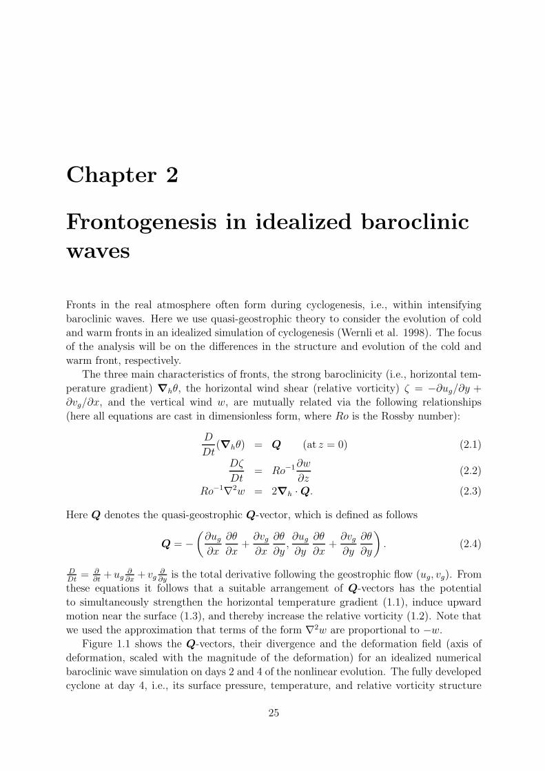
Fronts in the real atmosphere often form during cyclogenesis, i.e., within intensifying

baroclinic waves. Here we use quasi-geostrophic theory to consider the evolution of cold

and warm fronts in an idealized simulation of cyclogenesis (Wernli et al. 1998). The focus

of the analysis will be on the differences in the structure and evolution of the cold and

warm front, respectively.

The three main characteristics of fronts, the strong baroclinicity (i.e., horizontal tem-

perature gradient) ∇hθ, the horizontal wind shear (relative vorticity) ζ = −∂ug/∂y +

∂vg/∂x, and the vertical wind w, are mutually related via the following relationships

(here all equations are cast in dimensionless form, where Ro is the Rossby number):

D

Dt(∇hθ) = Q (at z = 0) (2.1)

Dζ

Dt= Ro−1∂w

∂z(2.2)

Ro−1∇2w = 2∇h ·Q. (2.3)

Here Q denotes the quasi-geostrophic Q-vector, which is defined as follows

Q = −(∂ug∂x

∂θ

∂x+∂vg∂x

∂θ

∂y,∂ug∂y

∂θ

∂x+∂vg∂y

∂θ

∂y

)

. (2.4)

DDt

= ∂∂t+ ug

∂∂x

+ vg∂∂y

is the total derivative following the geostrophic flow (ug, vg). From

these equations it follows that a suitable arrangement of Q-vectors has the potential

to simultaneously strengthen the horizontal temperature gradient (1.1), induce upward

motion near the surface (1.3), and thereby increase the relative vorticity (1.2). Note that

we used the approximation that terms of the form ∇2w are proportional to −w.Figure 1.1 shows the Q-vectors, their divergence and the deformation field (axis of

deformation, scaled with the magnitude of the deformation) for an idealized numerical

baroclinic wave simulation on days 2 and 4 of the nonlinear evolution. The fully developed

cyclone at day 4, i.e., its surface pressure, temperature, and relative vorticity structure

25

L

a)

L

b)

L

c)

LL

d)

LL

e)

LL

f)

Figure 2.1: Surface frontogenesis fields on day 2 (upper row) and day 4 (lower row) of the

nonlinear evolution of an idealized cyclone: Q-vectors (left), their divergence (middle)

and the axis of deformation scaled with the magnitude of the deformation (right). The

black contour denotes the approximate location of the surface fronts. Figure from Wernli

et al. (1998).

a) b)

Figure 2.2: Idealized extratropical cyclone at day 4 of its nonlinear evolution. Panel

(a) shows surface pressure and temperature, panel (b) the surface relative vorticity field.

Figure from Wernli et al. (1998).

is illustrated in Fig. 1.2. The amplitude of the Q-vectors and the deformation increases

during the nonlinear evolution, which indicates that the major part of the deformation is

associated with the flow of the intensifying low (and high) pressure systems. Both fields

show clear maxima along the evolving fronts. In the region of the cold front the Q-vectors

26

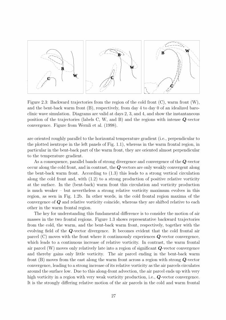
BB

CCWW

BB

CC

WW

BB

CC

WW

Figure 2.3: Backward trajectories from the region of the cold front (C), warm front (W),

and the bent-back warm front (B), respectively, from day 4 to day 0 of an idealized baro-

clinic wave simulation. Diagrams are valid at days 2, 3, and 4, and show the instantaneous

position of the trajectories (labels C, W, and B) and the regions with intense Q-vector

convergence. Figure from Wernli et al. (1998).

are oriented roughly parallel to the horizontal temperature gradient (i.e., perpendicular to

the plotted isentrope in the left panels of Fig. 1.1), whereas in the warm frontal region, in

particular in the bent-back part of the warm front, they are oriented almost perpendicular

to the temperature gradient.

As a consequence, parallel bands of strong divergence and convergence of the Q-vector

occur along the cold front, and in contrast, theQ-vectors are only weakly convergent along

the bent-back warm front. According to (1.3) this leads to a strong vertical circulation

along the cold front and, with (1.2) to a strong production of positive relative vorticity

at the surface. In the (bent-back) warm front this circulation and vorticity production

is much weaker – but nevertheless a strong relative vorticity maximum evolves in this

region, as seen in Fig. 1.2b. In other words, in the cold frontal region maxima of the

convergence of Q and relative vorticity coincide, whereas they are shifted relative to each

other in the warm frontal region.

The key for understanding this fundamental difference is to consider the motion of air

masses in the two frontal regions. Figure 1.3 shows representative backward trajectories

from the cold, the warm, and the bent-back warm front, respectively, together with the

evolving field of the Q-vector divergence. It becomes evident that the cold frontal air

parcel (C) moves with the front where it continuously experiences Q-vector convergence,

which leads to a continuous increase of relative vorticity. In contrast, the warm frontal

air parcel (W) moves only relatively late into a region of significant Q-vector convergence

and thereby gains only little vorticity. The air parcel ending in the bent-back warm

front (B) moves from the east along the warm front across a region with strong Q-vector

convergence, leading to a strong increase of its relative vorticity as the air parcels circulates

around the surface low. Due to this along-front advection, the air parcel ends up with very

high vorticity in a region with very weak vorticity production, i.e., Q-vector convergence.

It is the strongly differing relative motion of the air parcels in the cold and warm frontal

27

regions that is central for understanding the strikingly contrasting vorticity patterns of

cold and warm fronts, respectively.

28

Chapter 3

Frontal waves

According to the classical baroclinic instability theory (e.g., cast in form of the Eady

problem (Eady 1949), see lecture course on large-scale atmospheric dynamics), extra-

tropical cyclones evolve in baroclinic regions, i.e., regions with a large-scale, typically

meridionally oriented, horizontal temperature contrast. Surface fronts evolve then during

the non-linear growth of the baroclinic waves, i.e., of the low and high-pressure systems

(see, e.g., the idealized simulation discussed in the previous chapter), and are therefore

not a prerequisite for cyclogenesis.

In contrast, the classical “polar front theory” (e.g., Bjerknes 1919; Bjerknes and Sol-

berg 1922) describes cyclogenesis as an instability of a pre-existing surface front. Accord-

ing to this concept, the front is a prerequisite for cyclogenesis and not a consequence of

the non-linear evolution of cyclones. It is important to note that this “theory” has been

proposed based upon a synthesis of observations, and not based upon a physical theory of

why surface fronts become unstable. Only in 1990, instability analyses of surface fronts

have been proposed (see next section) that could satisfactorily explain the existence of

frontal waves that typically have a smaller wavelength than the larger-scale baroclinic

waves that emerge from classical baroclinic instability theory.

In reality, both types of instability exist: some cyclones develop in broad baroclinic

zones (and develop intense surface fronts during their nonlinear intensification), and oth-

ers emerge as waves on preexisting surface fronts (so-called “frontal wave cyclones”, see

Fig. 2.1). The latter category is often referred to as “secondary cyclones”, as they often

evolve on cold fronts that have evolved during a previous “primary” event of baroclinic

instability. In this chapter, we will first study the instability principles that explain the ex-

istence of frontal waves, and then discuss the key role of the deformation field for allowing

surface fronts to become unstable (or not). In the appendix, a generalized instability the-

orem is derived (within the quasi-geostrophic limit), which provides fundamental insight

into the characteristics of unstable flows.

29

3.1 Frontal instability analysis

In harmony with the instability theorem presented in the appendix, surface fronts are

unstable (i.e., can lead to emerging frontal wave cyclones) if they are either characterized

by a prefrontal surface warm band (e.g., realized trough warm-air advection ahead of the

surface front) or by a low-tropospheric band-like positive anomaly of potential vorticity

(produced most likely through cloud condensational diabatic processes along the surface

front). In 1990, two papers were published that study these mechanisms in isolation: the

instability of a prefrontal warm band (Schar and Davies 1990) and the instability of a

frontal low-level PV band (Joly and Thorpe 1990). Figure 2.2 presents the 2-dimensional

atmospheric flows that were used in these studies as the basic states for a linear instability

analysis.

Similar to the classical baroclinic wave instability analysis, the most unstable normal

mode was identified for the two basic states. In contrast to the Eady problem, these

instability problems cannot be solved analytically. For a set of normal mode wavelength,

numerical experiments were performed to quantify the respective growth rate. Figure

2.3 shows the numerically determined growth rate as a function of the along-front wave

number of the normal mode disturbance for the basic state examined by Joly and Thorpe

(1990). They found maximum growth for an along-front wave number of l = 8 · 10−6m−1,

which corresponds to a wavelength of about 800 km. This wavelength is about 4-5 times

smaller than the wavelength of the most unstable normal mode of the classical Eady

problem of baroclinic instability, which indicates the presence of a fundamentally dif-

Figure 3.1: Examples of North Atlantic frontal waves. (a) Surface chart at 12 UTC 1

December 1982 (reduced surface pressure, contour interval of 4 hPa); (b) surface chart at

18 UTC 20 October 1989; and (c) PV on 900 hPa at the same time as (b), values larger

than 0.75 pvu are stippled in grey. Figure from Joly and Thorpe (1990).

30

Figure 3.2: Vertical cross-sections illustrating the surface frontal basic states used in the

studies by (left) Schar and Davies (1990) and (right) Joly and Thorpe (1990). The panels

on the left show (top) potential temperature (thick lines, contour interval 2K) and along-

frontal wind (thin lines, contour interval 3.3ms−1), and (bottom) relative vorticity (in

units of f). Panels on the right show (top) PV (contour interval 0.2 pvu) and (bottom)

potential temperature (dashed lines, contour interval 4K) and along-frontal wind (solid

and short-dashed lines at 4ms−1 intervals).

Figure 3.3: Normal mode growth rate as a function of the along-front wave number l for

the basic state shown in Fig. 2.2 (right). Figure from Joly and Thorpe (1990).

ferent physical instability mechanism. Note also that the relatively short wavelength

qualitatively agrees well with the typical distance between multiple frontal waves on an

elongated front (see Fig. 2.1).

Also the structure of the most unstable normal mode of the frontal instability problem

(see Fig. 2.4) is significantly different from the normal mode structure of the Eady prob-

31

Figure 3.4: Structure of the most unstable normal mode at the surface for the basic

state shown in Fig. 2.2 (left). Shown are the perturbations of pressure (upper panel) and

temperature (bottom panel). The small diagrams on the right illustrate the basic state

profiles of pressure and temperature perpendicular to the front. Figure from Schar and

Davies (1990).

lem. The normal mode is shallow as its amplitude decays with altitude. In contrast, the

most unstable normal mode of the Eady problem had equal amplitude at the surface and

the tropopause. Figure 2.4 shows that the surface temperature perturbation associated

with the normal mode vanishes at the location of the basic state’s surface temperature

maximum and exhibits two wave trains shifted by π/2 relative to each other. It is these

temperature wave trains on both sides of the surface front that constructively interact

to produce the frontal wave instability – in contrast to the Eady problem, where a ver-

tical interaction of wave trains at the surface and the tropopause leads to the baroclinic

instability.

3.2 Frontal instability and deformation

The highly idealized studies discussed in the previous section show that surface fronts can

be unstable. Practical experience (e.g., of forecasters) however indicates that many surface

fronts remain stable and do not show the evolution of unstable frontal wave cyclones. In

other cases, several waves form initially (see Fig. 2.1a), but then only one of the nascent

waves intensifies into a major cyclone whereas the other wave disturbances decay. The

dynamical reasons for this strongly differing behavior of surface fronts and frontal waves

is not yet fully understood. According to the theory by Bishop and Thorpe (1994),

environmental deformation is a key for understanding the evolution of frontal waves.

One the one hand, deformation is essential for producing surface fronts in the first place.

32

Figure 3.5: Temporal evolution for two North Atlantic frontal wave cases in January

1995 (denoted as La and Lu) of (a) the vorticity waviness and (b) the environmental

deformation. Figure from Renfrew et al. (1997).

Therefore, a surface flow with strong deformation is important for the formation of fronts,

which is a prerequisite for the subsequent formation of frontal waves. On the other

hand, Bishop and Thorpe (1994) argued that a sustained deformation field is suppressing

frontal instability, i.e., the evolution of intensifying frontal waves. It follows that in order

to produce frontal waves, the ideal flow setting is transient (i.e., evolves in time), with

strong deformation initially to produce the front followed by a decrease of the strength of

the deformation in order to allow the frontal instability to develop.

Renfrew et al. (1997) tested this hypothesis by investigating a set of developing and

non-developing frontal waves. For each case, they quantified the “vorticity waviness”

along the surface front, which they defined as the difference between the peak vorticity

and the averaged vorticity along the front. For instance, a uniform along-frontal vorticity

band has zero waviness. They then examined the temporal evolution of the waviness with

respect to the temporal evolution of the environmental deformation (see Fig. 2.5). For

33

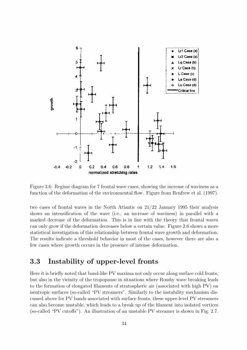
Figure 3.6: Regime diagram for 7 frontal wave cases, showing the increase of waviness as a

function of the deformation of the environmental flow. Figure from Renfrew et al. (1997).

two cases of frontal waves in the North Atlantic on 21/22 January 1995 their analysis

shows an intensification of the wave (i.e., an increase of waviness) in parallel with a

marked decrease of the deformation. This is in line with the theory that frontal waves

can only grow if the deformation decreases below a certain value. Figure 2.6 shows a more

statistical investigation of this relationship between frontal wave growth and deformation.

The results indicate a threshold behavior in most of the cases, however there are also a

few cases where growth occurs in the presence of intense deformation.

3.3 Instability of upper-level fronts

Here it is briefly noted that band-like PV maxima not only occur along surface cold fronts,

but also in the vicinity of the tropopause in situations where Rossby wave breaking leads

to the formation of elongated filaments of stratospheric air (associated with high PV) on

isentropic surfaces (so-called “PV streamers”. Similarly to the instability mechanism dis-

cussed above for PV bands associated with surface fronts, these upper-level PV streamers

can also become unstable, which leads to a break up of the filament into isolated vortices

(so-called “PV cutoffs”). An illustration of an unstable PV streamer is shown in Fig. 2.7.

34

Figure 3.7: Water vapour satellite image at 06 UTC 29 April 1996. Figure from Fehlmann

(1997).

Water vapor satellite images are ideally suited to observe the formation and potential

break-up of PV streamers.

35

·

36

Chapter 4

Stratosphere-troposphere exchange

4.1 STE processes

The tropopause is classically thought as an “impermeable transport barrier” between

the troposphere and the stratosphere. Consider the tropopause defined as an isosurface

of potential vorticity (PV), e.g., the 2-pvu tropopause. For an adiabatic flow, PV is

materially conserved:D

DtPV = 0 , (4.1)

and, as a consequence, a stratospheric air parcel with PV> 2 pvu stays always in the

stratosphere independent of its motion. The same applies for tropospheric air parcels as

long as the flow is adiabatic. Therefore, there is no stratosphere-troposphere exchange

(STE) for an adiabatic flow – if we define the tropopause as a PV-isosurface.

The PV framework nicely indicates that STE can only occur if frictional forces and/or

latent heating are occurring. Only these processes have the potential to modify an air

parcel’s PV and therefore transfer it from the stratosphere to the troposphere, or vice

versa. The full equation for the material change of PV is:

D

DtQ =

1

ρη·∇θ + 1

ρ∇θ · (∇∧ F) . (4.2)

Here θ denotes the diabatic heating rate due to latent heating and cooling in clouds and

due to radiation (in K s−1), and F the sum of all non-conservative forces (e.g., friction

due to turbulence). It becomes evident that STE, i.e., the material non-conservation of

PV is linked either to latent heating/cooling processes or turbulence near the tropopause.

These processes typically occur on the mesoscale.

Historically, it was after the nuclear bomb tests in the stratosphere in the 1960ies,

that radioactive material from the bombs was observed at the surface. This was a clear

indication that the tropopause is not a strict barrier and that STE indeed occurs (e.g.,

Danielsen 1968). STE directly impacts on atmospheric composition, chemistry, and cli-

mate: since it transports air masses between chemically differing reservoirs (e.g., high

ozone, low water vapour and low carbonmonoxide in the stratosphere and vice versa in

37

Figure 4.1: Aircraft observations in a tropopause fold, the dashed line with arrows indi-

cates the path of the aircraft. Left: ozone concentrations (dashed lines) and the 1-pvu

isoline (solid line labeled with 100). Right: isolines of the bulk Richardson number (val-

ues less than 1 indicate regions where turbulence is likely to occur). Figure from Shapiro

(1978).

the troposphere) it changes the oxidative capacity of the troposphere and potentially also

affects the climate system because ozone and water vapour are potent greenhouse gases.

STE down to the surface can also contribute to enhanced ozone levels at the ground and

affect plant and human physiology. However, since early studies on STE, quantification

of the relative role of the different physical processes that can lead to STE (e.g., cloud

diabatic heating, radiative heating/cooling, turbulence) remains an open issue. Early air-

craft observations near tropopause folds (see Fig. 4.1) showed that isolines of ozone do not

coincide perfectly with isolines of PV (left panel), which indicates that in certain regions,

the tropopause is “leaky”. Measurements indicate that in these regions the Richardson

number is small (due to the strong vertical gradient of the horizontal wind), pointing to

the possibilty for STE to occur associated with clear-air turbulence. In other situations,

diabatic heating/cooling might be strongly involved in STE, for instance in cases with

a very strong vertical humidity gradient and/or the presence of clouds just below the

tropopause (e.g., Wirth and Egger 1999; Bourqui 2006).

When considering STE processes, it is very important to keep in mind that the extra-

tropical tropopause is a highly dynamic interface. An arbitrary snapshot of the structure

of the tropopause reveals remarkable structures with tropopause folds, regions where the

tropopause is particularly steep and anomalously high or low (Fig. 4.2). It is typically in

the regions where the tropopause height deviates from the climatological mean position,

where STE is likely to occur, e.g, due to turbulence in regions with a steep tropopause,

38

Figure 4.2: Vertical cross section at a specific time of the potential vorticity structure

from the South to the North Pole. Negative PV values in the Southern Hemisphere are

shown as positive values. The 2-pvu tropopause is highlighted by a black line.

due to latent heating in clouds in regions with an anomalously low tropopause, and due

to radiative effects in regions with an anomalously high tropopause.

4.2 Methods to identify STE

Several methods have been developed to identify and quantify STE. Early methods were

Eulerian and in essence considered the instantaneous vertical velocity relative to the

motion of the tropopause. With this concept, STE occurs at a certain point if the vertical

motion of an air parcel at the tropopause is larger than the motion of the tropopause itself.

Numerically, this method is difficult to implement (small difference of two larger terms)

and can lead to very spurious results. Also, this method cannot provide information about

the orgin and destination of STE airmasses.

Here the Lagrangian approach is of advantage (Wernli and Bourqui 2002; Stohl et

al. 2003; Skerlak et al. 2014). It is based upon the calculation of a large number of

air parcel trajectories. In this framework, STE occurs whenever PV along a trajectory

changes from more than 2 pvu to less than 2 pvu, or vice versa. It is straightforward

to distinguish between stratosphere-to-troposphere transport (STT) and troposphere-to-

stratosphere transport (TST). Also, it is possible to quantify, for instance, how long

an STT air parcel remains in the troposphere before returning to the stratosphere. In

terms of chemical impact, an STT event is only relevant if the originally stratospheric

air parcel remains long enough in the troposphere, such that turbulent mixing can occur,

which eventually transfers the stratospheric compositions (e.g., high ozone values) into the

troposphere. If the air parcel returns quickly to the stratosphere without mixing, then the

39

Figure 4.3: Overview on STE processes (see text for details). The black line shows the

instantaneous 2-pvu/380-K tropopause (dashed is its climatological mean position). Blue

colors denote the overworld, yellow the lowermost stratosphere, red the troposphere, and

brown the boundary layer. Figure from Stohl et al. (2003).

STT has no chemical implications. And finally, the Lagrangian approach provides insight

where STE air parcels are coming from and where they are going to. The term “deep STE”

has been introduced for STE air parcels that rapidly travel from the stratosphere into the

planetary boundary layer (deep STT) or vice versa (deep TST). Such events, although

they are comparatively rare, can bring air parcels in contact that are characterized by

strongly differing chemical composition (e.g., polluted boundary layer air and “clean”

stratospheric air).

Figure 4.3 summarizes some important aspects of STE, which have been identified with

this Lagrangian approach. The figure shows different STE air parcels (green trajectories).

The warm conveyor belt (WCB) shows an example of deep TST, where the air parcel

first ascends rapidly within a moist WCB, enters an upper-level ridge (note the upward

distorted tropopause), and then gains PV and enters the lower stratosphere. Also shown

in this figure are arrows indicating the so-called large-scale Brewer-Dobson circulation

with ascent in the tropics, a poleward transport in the stratosphere, and descent in the

polar regions (e.g., Holton et al. 1995). Note that this large-scale circulation is much

slower and involves less mass than the many transient STE events at the extratropical

tropopause.

40

Figure 4.4: Climatology of STT in Northern Hemisphere winter (DJF, left) and summer

(JJA, right). The upper panels show the STT mass flux at the level of the tropopause;

the lower panels show the STT mass flux into the planetary boundary layer. Figures from

Skerlak et al. (2014).

4.3 Climatology of STE

This Lagrangian method can be used to compile a global climatology of STE, based upon

the calculation of millions of trajectories (Skerlak et al. 2014). Upper panels in Fig. 4.4

shows the STT (i.e., downward) mass flux in the Northern Hemisphere winter and summer,

respectively. STT is comparatively weak in the tropics, except for a summer maximum

in the Indian Ocean, and attains the largest values (green, yellow and red colors) in the

extratropical storm track regions, in particular in winter over the North Pacific and North

Atlantic. There is substantial zonal variability, in particular in the Northern Hemisphere,

with summer peaks over Eurasia. In the Southern Hemisphere interesting peaks occur

over South America in summer and to the weat and east of Australia in winter. Only

a very small fraction of these trajectories reach the boundary layer and are therefore

classified as deep STT. The lower panels in Fig. 4.4 show where deep STT air parcels

enter the boundary layer, again in the two seasons DJF and JJA. It becomes evident that

deep STT is most frequent in mountaineous regions, i.e., over the Rockies, the Himalaya,

and the Andes. In winter, deep STT also occurs over the ocean near 30-40◦ latitude.

These figures show that in high mountain regions it is most likely for stratospheric ozone

to reach down to the surface. In most low-elevations sites, however, stratospheric ozone

hardly ever contributes to the observed boundary layer concentrations.

41

Figure 4.5: Tracer-tracer correlation plot with CO and ozone from aircraft observations

in the upper troposphere and lower stratosphere over Europe in February 2003. Figure

from Hoor et al. (2004).

4.4 STE and atmospheric composition

It is plausible that STE leads to a weakening of the vertical gradients in chemical tracer

concentrations across the tropopause. Considering, carbonmonoxide (CO) and ozone

(O3), the pure stratosphere would be characterized by less than 40 ppb of CO and more

than 600 ppb of O3, whereas pure (polluted) tropospheric air would be characterized

by more than 100 ppb ov CO and less than 100 ppb of O3. Aircraft observations in the

region at and above the tropopause, however, show a more gradual transition between pure

tropospheric and stratospheric air masses (Fig. 4.5). The figure shows aircraft observations

of CO and O3 from the field experiment SPURT obtained above Europe between about

8 and 14 km altitude on 15/16 February 2003. This diagram is known as tracer-tracer

correlation plot and indicates the existence of a layer above the tropopause with air masses

that are intermediate between pure tropospheric and pure stratopsheric (e.g., with a CO

concentration of 60 ppb and O3 values of 300 ppb). Such concentrations can occur due to

TST (which imports high CO values into the lowermost stratosphere) and the subsequent

mixing of TST air masses with the surrounding stratosphere (characterized by high O3

values). Therefore, Fig. 4.5 provides experimental evidence for the existence of STE

processes (withouth STE, the tracer-tracer correlation plot would only show values in the

upper left and lower right corner).

42

Appendix A

Instability theorem after Eliassen

Consider an idealized atmosphere sandwiched between two horizontal planes at z = 0

(the surface) and z = zT (the tropopause). A channel atmosphere is considered, i.e., we

assume periodicity in the x-direction. Along the y-axis the channel extends to ±a. In the

limit of quasi-geostrophic (QG) dynamics of a dry atmosphere, the following equations

describe the evolution of the system:

Dg

Dt(∆ψ + βy) = 0 (A.1)

Dg

Dt

(∂ψ

∂z

)

= 0, z = 0, zT . (A.2)

Equation (A.1) describes the conservation of QG potential vorticity q = ∆ψ + βy in the

interior of the atmosphere, and equation (A.2) the conservation of potential temperature

θ = ∂ψ

∂zon the two horizontal bounding surfaces.

We now linearize the equations with respect to zonally uniform zonal flow. All variables

are decomposed into a zonally uniform basic state component and a small perturbation,

according to ug = u+ u′, vg = v′, ψ = ψ+ψ′, and q = q+ q′. This leads to the linearized

versions of equations (A.1, A.2):

(∂

∂t+ u

∂

∂x

)

q′ +∂q

∂yv′ = 0 (A.3)

(∂

∂t+ u

∂

∂x

)∂ψ′

∂z− ∂u

∂zv′ = 0, z = 0, zT . (A.4)

Introducing η′ as the north-south displacement of an air parcel

(∂

∂t+ u

∂

∂x

)

η′ := v′ (A.5)

and using the notationDt =(∂∂t+ u ∂

∂x

)we can recast equations (A.3, A.4) in the following

43

form:

Dt

[

q′ +∂q

∂yη′]

= 0 (A.6)

Dt

[∂ψ′

∂z− ∂u

∂zη′]

= 0, z = 0, zT . (A.7)

Assuming that the perturbation can be decomposed into a superposition of periodic nor-

mal modes yields the following relationships:

q′ +∂q

∂yη′ = 0 (A.8)

∂ψ′

∂z− ∂u

∂zη′ = 0, z = 0, zT . (A.9)

We next consider the two expressions Dt(uz12η′2) and Dt(qy

12η′2). Both terms can be

reformulated as follows, using (A.8) and (A.9):

Dt(uz1

2η′2) = uzη

′Dtη′ = ψ′

zv′, z = 0, zT (A.10)

Dt(qy1

2η′2) = qyη

′Dtη′ = −q′v′. (A.11)

Integrating (A.11) over the entire atmosphere with the volume V yields the following re-

lationship (using integration by parts and considering that terms of the form∫

V∂∂x(...)dV

vanish due to the imposed peridicity in x):∫

V

Dt(qy1

2η′2)dV = −

∫

V

q′v′dV

= −∫

V

ψ′x(ψ

′xx + ψ′

yy + ψ′zz)dV

= ... = −[∫

x

∫

y

v′ψ′zdxdy

]zT

z=0

= −[∫

x

∫

y

Dt(uz1

2η′2)dxdy

]zT

z=0

.(A.12)

Again due to the periodicity in x if follows that∫

V

Dt(...)dV =

∫

V

∂

∂t(...)dV =

∂

∂t

∫

V

(...)dV (A.13)

and therefore, (A.12) yields:

∂

∂t

∫

x

∫

y

∫

z

∂q

∂y

1

2η′2dz

︸ ︷︷ ︸

R1

+∂u

∂z

1

2η′2|z=zT

︸ ︷︷ ︸

R2

− ∂u

∂z

1

2η′2|z=0

︸ ︷︷ ︸

R3

dxdy = 0. (A.14)

In case of an instability the north-south displacements associated with the perturbation

grow continuously, i.e.,∂

∂t

∫

V

1

2η′2dV > 0. (A.15)

44

According to (A.14) this is only possible if all terms Ri, i = 1, 2, 3 are equal to zero

or if they mutually compensate. Equation (A.14) therefore indicates several options for

instability:

• the Eady problem: q = const.; ∂u∂z

= const.

⇒ R1 = 0;R2 = R3

• the Charney problem: zT → ∞; ∂q

∂y= β = const.; ∂u

∂z= const.

⇒ R2 = 0;∫

x

∫

y(R1 − R3)dxdy = 0

• classical barotropic instability: ∂u∂z

= 0

⇒ R2 = R3 = 0;∫

x

∫

yR1dxdy = 0. This signifies that ∂q

∂yattains both positive and

negative values in the interior of the atmosphere, which only occurs if the PV field

exhibits a local maximum (or minimum) in the interior of the atmosphere. This is

the case, for instance, in situations with an along-frontal band of high PV (see, e.g.,

Joly and Thorpe 1990).

• warmband instability (cf. Schar and Davies 1990): zT → ∞; q = const.

⇒ R1 = R2 = 0;∫

x

∫

yR3dxdy = 0. This signifies that ∂u

∂z= −∂θ

∂yattains both positive

and negative values at the surface, which is the case only if the surface temperature

field has a local maximum (or minimum). This occurs, for instance, in situations with

a band of increased temperature parallel to a surface cold front.

45

References

Bishop, C. H., and A. J. Thorpe, 1994. Frontal wave stability during moist deformation fronto-

genesis. 2: The suppression of nonlinear-wave development. J. Atmos. Sci., 51, 874-888.

Bjerknes, J., 1919. On the structure of moving cyclones. Geofys. Publ., 1(2), 1-8.

Bjerknes, J. and H. Solberg, 1922. Life cycles of cyclones and the polar front theory of atmo-

spheric circulation. Geofys. Publ., 3(1), 3-18.

Bourqui, M. S., 2006. Stratosphere-troposphere exchange from the Lagrangian perspective: a

case study and method sensitivities. Atmos. Chem. Phys., 6, 2651-2670.

Danielsen, E., 1968. Stratospheric-tropospheric exchange based on radioactivity, ozone and

potential vorticity. J. Atmos. Sci., 25, 502-518.

Eady, E. T., 1949. Long waves and cyclone waves. Tellus, 1, 33-52.

Fehlmann, R., 1997. Dynamics of seminal PV elements. Ph. D. thesis, Dissertation Nr. 12229

ETH Zurich, 143pp.

Holton, J. R., P. H. Haynes, M. E. McIntyre, A. R. Douglass, R. B. Rood, and L. Pfister, 1995.

Stratosphere-troposphere exchange. Rev. Geophys., 33, 403-440.

Hoor, P., C. Gurk, D. Brunner, M. I. Hegglin, H. Wernli, and H. Fischer, 2004. Seasonality

and extent of extratropical TST derived from in-situ CO measurements during SPURT.

Atmos. Chem. Phys., 4, 1427-1442.

Hoskins, B. J., M. E. McIntyre, and A. W. Robertson, 1985. On the use and significance of

isentropic potential vorticity maps. Quart. J. Roy. Meteorol. Soc., 111, 877-946.

Joly, A., and A. J. Thorpe, 1990. Frontal instability generated by tropospheric potential vorticity

anomalies. Quart. J. Roy. Meteorol. Soc., 116, 525-560.

Renfrew, I. A., A. J. Thorpe, and C. H. Bishop, 1997. The role of the environmental flow in the

development of secondary frontal cyclones. Quart. J. Roy. Meteorol. Soc., 123, 1653-1675.

Schar, C., and H. C. Davies, 1990. An instability of mature cold fronts. J. Atmos. Sci., 47,

929-950.

Skerlak, B., M. Sprenger, and H. Wernli, 2014. A global climatology of stratosphere-troposphere

exchange using the ERA-Interim dataset from 1979 to 2011. Atmos. Chem. Phys., 14,

913-937.

Stohl, A., P. Bonasoni, P. Cristofanelli, W. Collins, J. Feichter, A. Frank, C. Forster, E. Gera-

sopoulos, H. Gaggeler, P. James, A. S. Kentarchos, H. Kromp-Kolb, B. Kruger, C. Land,

J. Meloen, A. Papayannis, A. Priller, P. Seibert, M. Sprenger, G. J. Roelofs, H. E. Scheel,

C. Schnabel, P. Siegmund, L. Tobler, T. Trickl, H. Wernli, V. Wirth, P. Zanis, and C. Zere-

fos, 2003. Stratosphere-troposphere exchange: A review, and what we have learned from

STACCATO. J. Geophys. Res., 108, 8516, doi:10.1029/2002JD002490.

Wernli, H., and M. Bourqui, 2002. A Lagrangian 1-year climatology of (deep) cross-tropopause

exchange in the extratropical Northern Hemisphere. J. Geophys. Res., 107, 4021, doi:10.

1029/2001JD000812.

46

Wernli, H., R. Fehlmann and D. Luthi, 1998. The effect of barotropic shear on upper-level in-

duced cyclogenesis: semigeostrophic and primitive equation numerical simulations. J. At-

mos. Sci., 55, 2080-2094.

47