Lecture8-Wires-Transistorsbwrcs.eecs.berkeley.edu/Classes/icdesign/ee141_s10/Lectures/Lecture8... ·...
20
EE141 1 EE141 EECS141 1 Lecture #8 EE141 EECS141 2 Lecture #8 Hw 3 due today – HW 4 to be posted No Lab next week Extra review session Th at 6:30pm
Transcript of Lecture8-Wires-Transistorsbwrcs.eecs.berkeley.edu/Classes/icdesign/ee141_s10/Lectures/Lecture8... ·...
EE141
1
EE141 EECS141 1 Lecture #8
EE141 EECS141 2 Lecture #8
Hw 3 due today – HW 4 to be posted No Lab next week Extra review session Th at 6:30pm
EE141
2
EE141 EECS141 3 Lecture #8
Last lecture Logical Effort + Wires
Today’s lecture Wiring (cntd) – Transistor models
Reading (Ch 3, 4)
EE141 EECS141 4 Lecture #8
EE141
3
EE141 EECS141 5 Lecture #8
EE141 EECS141 6 Lecture #8
EE141
4
EE141 EECS141 7 Lecture #8
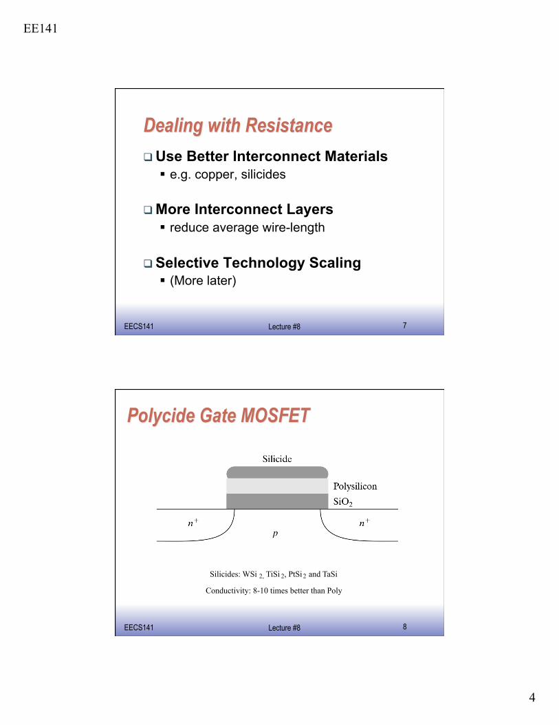
Use Better Interconnect Materials e.g. copper, silicides
More Interconnect Layers reduce average wire-length
Selective Technology Scaling (More later)
EE141 EECS141 8 Lecture #8
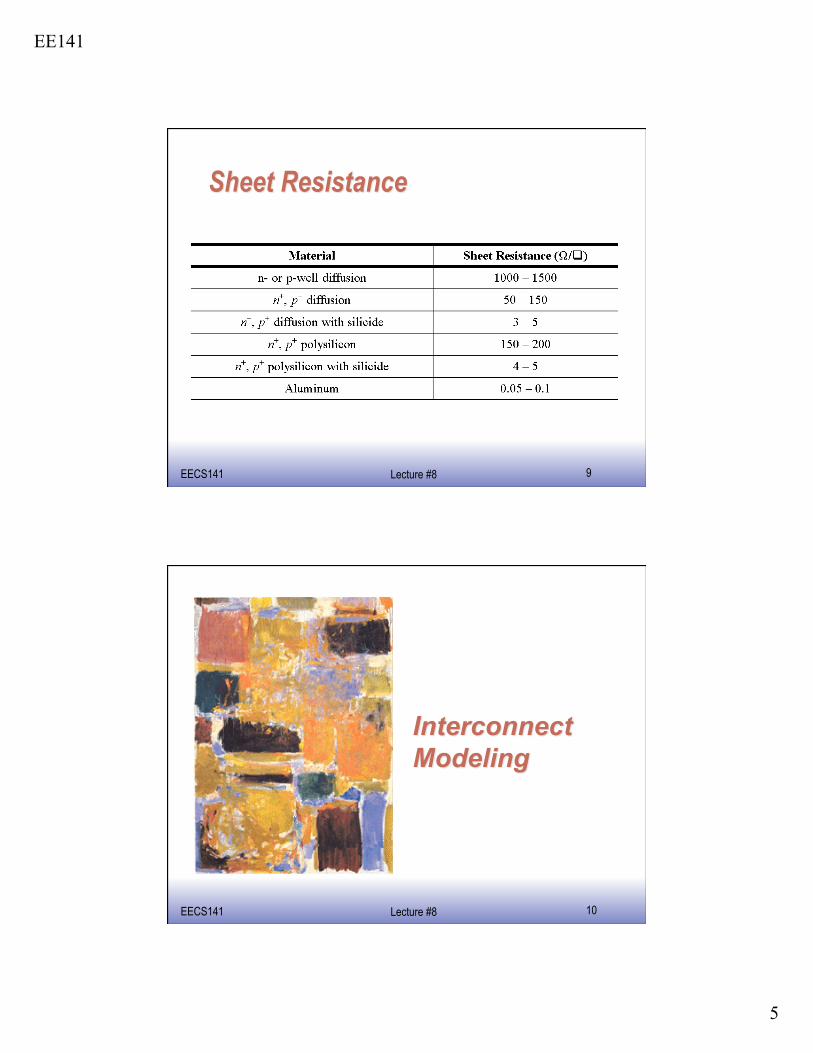
Silicides: WSi 2, TiSi 2 , PtSi 2 and TaSi Conductivity: 8-10 times better than Poly
EE141
5
EE141 EECS141 9 Lecture #8
EE141 EECS141 10 Lecture #8
EE141
6
EE141 EECS141 11 Lecture #8
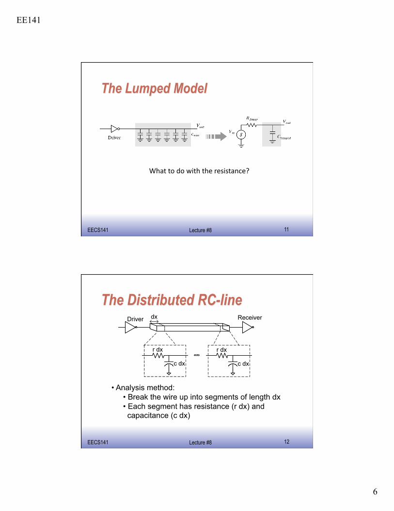
What to do with the resistance?
EE141 EECS141 12 Lecture #8
• Analysis method: • Break the wire up into segments of length dx • Each segment has resistance (r dx) and capacitance (c dx)

EE141
7
EE141 EECS141 13 Lecture #8
The diffusion equation
EE141 EECS141 14 Lecture #8
EE141
8
EE141 EECS141 15 Lecture #8
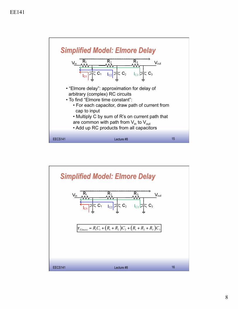
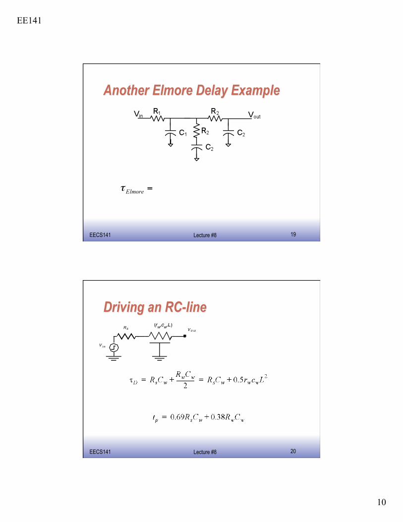
• “Elmore delay”: approximation for delay of arbitrary (complex) RC circuits • To find “Elmore time constant”:
• For each capacitor, draw path of current from cap to input • Multiply C by sum of R’s on current path that are common with path from Vin to Vout • Add up RC products from all capacitors
EE141 EECS141 16 Lecture #8
EE141
9
EE141 EECS141 17 Lecture #8
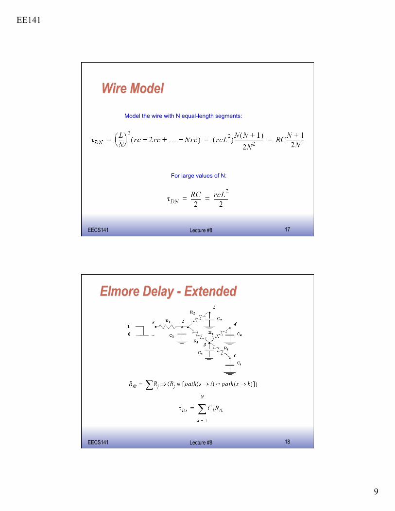
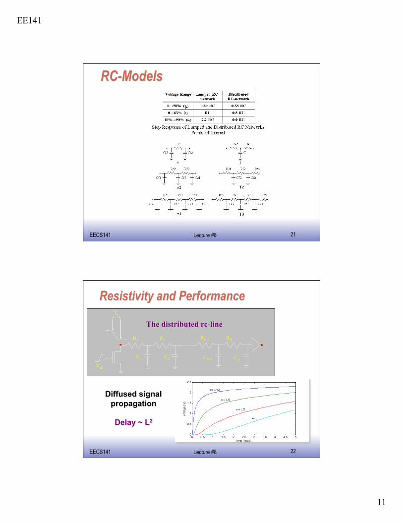
Model the wire with N equal-length segments:
For large values of N:
EE141 EECS141 18 Lecture #8
EE141
10
EE141 EECS141 19 Lecture #8
EE141 EECS141 20 Lecture #8
EE141
11
EE141 EECS141 21 Lecture #8
EE141 EECS141 22 Lecture #8
CN-1 CN C2
R1 R2
C1
Tr
Vin
RN-1 RN
EE141
12
EE141 EECS141 23 Lecture #8
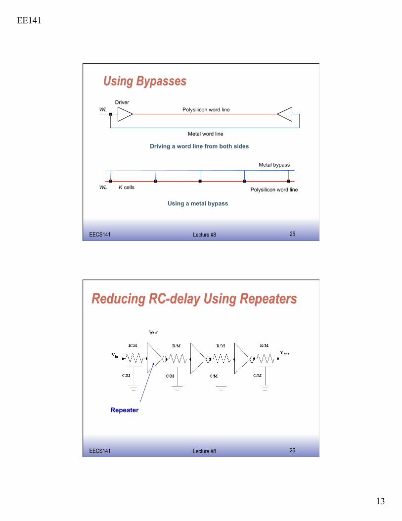
Challenges No further improvements to be expected after the
introduction of Copper (superconducting, optical?) Design solutions
Use of fat wires Efficient chip floorplanning Insert repeaters
( ) out w w d out d w w d C R C R C R C R T + + + = 693 . 0 377 . 0
EE141 EECS141 24 Lecture #8
# of metal layers is steadily increasing due to:"• Increasing die size and device count: we need more wires and longer wires to connect everything
• Rising need for a hierarchical wiring network; local wires with high density and global wires with low RC
0.25 µm wiring stack
EE141
13
EE141 EECS141 25 Lecture #8
Driver Polysilicon word line
Polysilicon word line
Metal word line
Metal bypass
Driving a word line from both sides
Using a metal bypass
WL
WL K cells
EE141 EECS141 26 Lecture #8
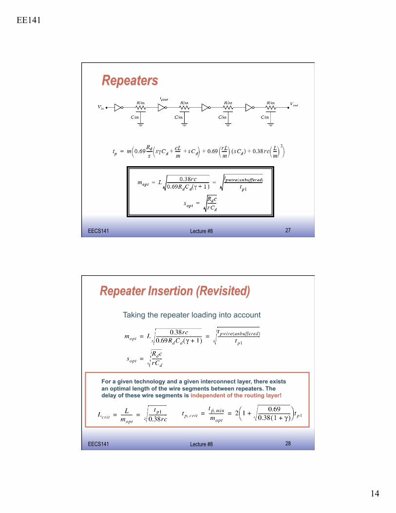
Repeater
EE141
14
EE141 EECS141 27 Lecture #8
EE141 EECS141 28 Lecture #8
Taking the repeater loading into account
EE141
15
EE141 EECS141 29 Lecture #8
What do digital IC designers need to know?
EE141 EECS141 30 Lecture #8
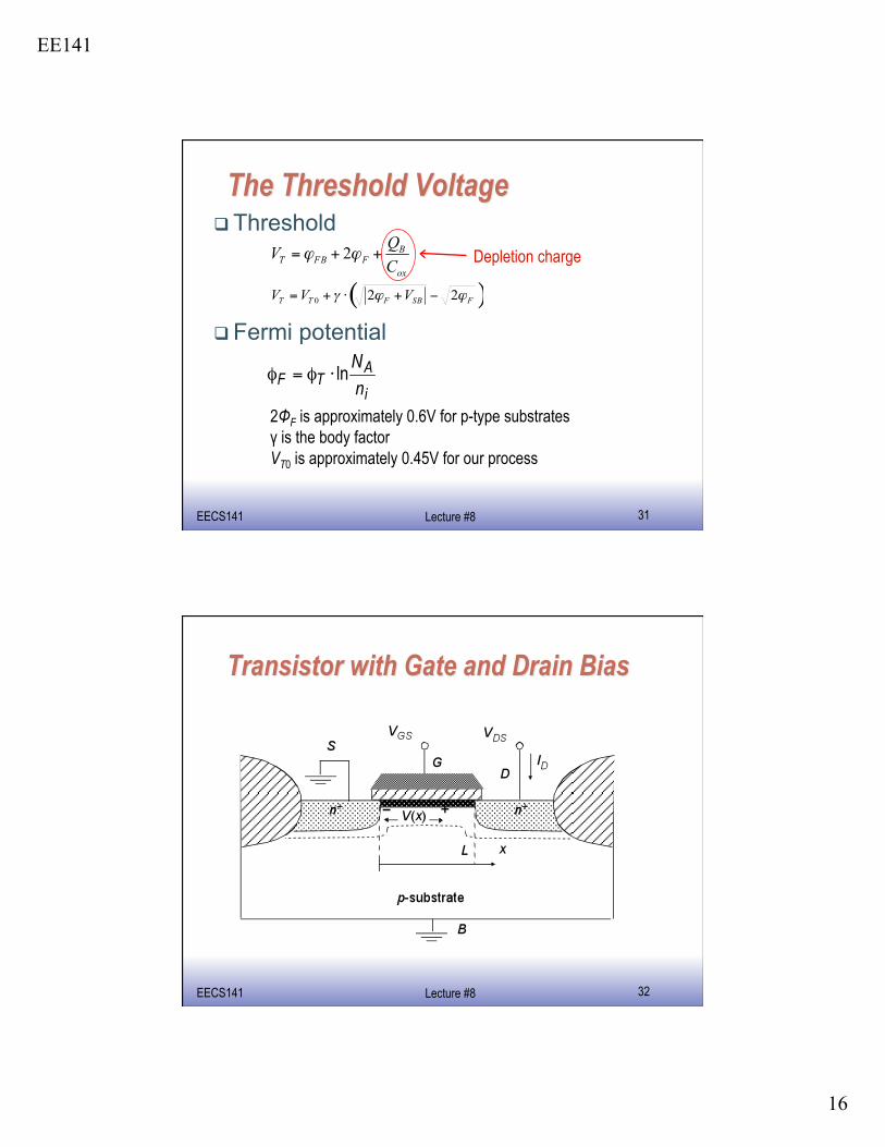
With positive gate bias, electrons pulled toward the gate With large enough bias, enough electrons will be pulled to "invert"
the surface (p→n type) Voltage at which surface inverts: “magic” threshold voltage VT
EE141
16
EE141 EECS141 31 Lecture #8
Threshold
Fermi potential
2ΦF is approximately 0.6V for p-type substrates γ is the body factor VT0 is approximately 0.45V for our process
Depletion charge
EE141 EECS141 32 Lecture #8
EE141
17
EE141 EECS141 33 Lecture #8
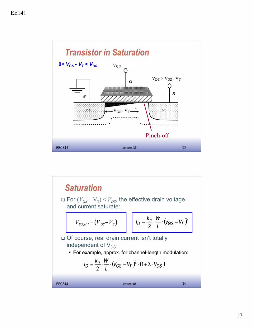
Pinch-off
0< VGS - VT < VDS
EE141 EECS141 34 Lecture #8
For (VGS – VT) < VDS, the effective drain voltage and current saturate:
’
Of course, real drain current isn’t totally independent of VDS For example, approx. for channel-length modulation:
’
EE141
18
EE141 EECS141 35 Lecture #8
Cutoff: VGS -VT< 0
Linear (Resistive): VGS-VT > VDS
Saturation: 0 < VGS-VT < VDS
’
’
EE141 EECS141 36 Lecture #8
Quadratic Relationship
0 0.5 1 1.5 2 2.5 0
1
2
3
4
5
6 x 10 -4
VGS= 2.5 V
VGS= 2.0 V
VGS= 1.5 V
VGS= 1.0 V
Resistive Saturation
VDS = VGS - VT
VDS (V)
I D (A
)
EE141
19
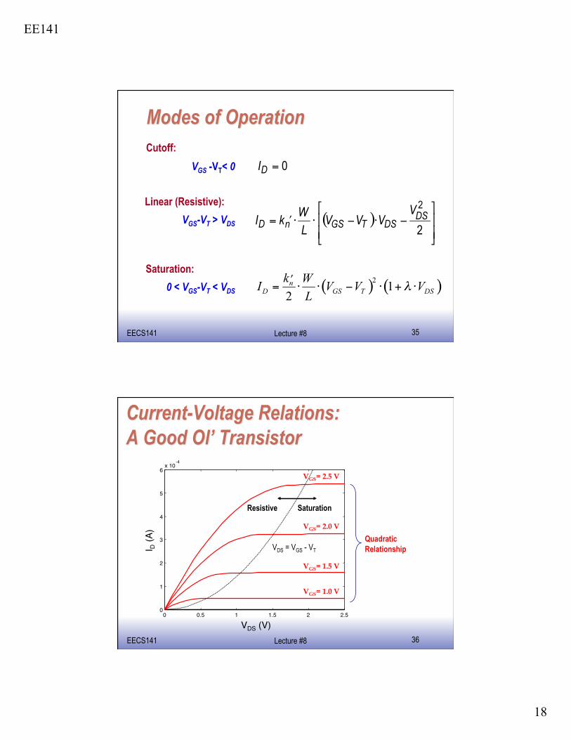
EE141 EECS141 37 Lecture #8
Linear Relationship
-4
0 0.5 1 1.5 2 2.5 0
0.5
1
1.5
2
2.5 x 10
VGS= 2.5 V
VGS= 2.0 V
VGS= 1.5 V
VGS= 1.0 V
Early Saturation
VDS (V)
I D (A
)
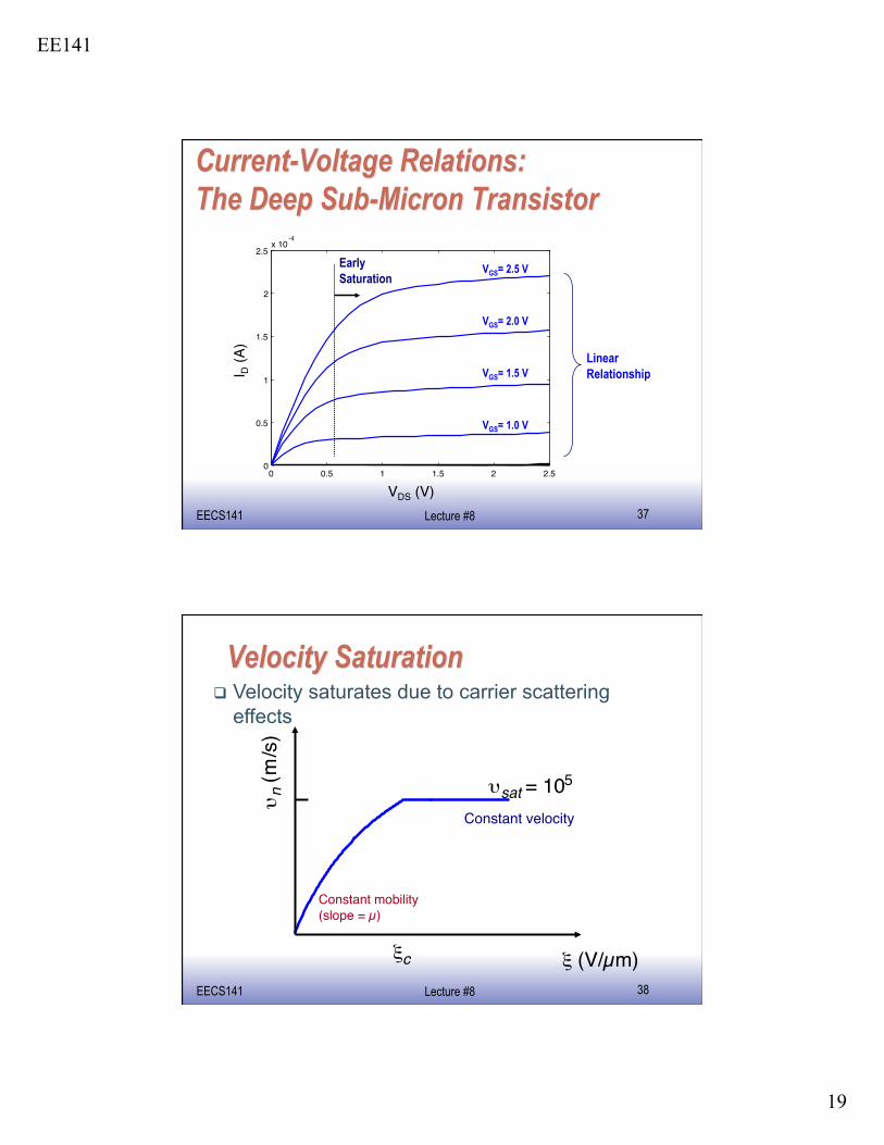
EE141 EECS141 38 Lecture #8
ξ (V/µm)
υ n
( m / s
)
υ sat = 10 5
Constant mobility "(slope = µ)
Constant velocity
ξ c
Velocity saturates due to carrier scattering effects
EE141
20
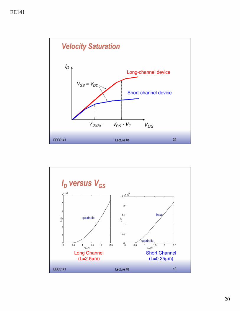
EE141 EECS141 39 Lecture #8
I D Long-channel device
Short-channel device
V DS V DSAT V GS - V T
V GS = V DD
EE141 EECS141 40 Lecture #8
0 0.5 1 1.5 2 2.5 0
1
2
3
4
5
6 x 10 -4
V GS (V)
I D (A
)
0 0.5 1 1.5 2 2.5 0
0.5
1
1.5
2
2.5 x 10 -4
V GS (V)
I D (A)
quadratic
quadratic
linear
Long Channel"(L=2.5µm)
Short Channel"(L=0.25µm)