Lecture7 xing fei-fei
98
Eric Xing © Eric Xing @ CMU, 2006-2010 1 Machine Learning Data visualization and dimensionality reduction Eric Xing Lecture 7, August 13, 2010
-
Upload
tianlu-wang -
Category
Automotive
-
view
389 -
download
0
Transcript of Lecture7 xing fei-fei
Eric Xing © Eric Xing @ CMU, 2006-2010 1
Machine Learning
Data visualization and dimensionality reduction
Eric Xing
Lecture 7, August 13, 2010
Eric Xing © Eric Xing @ CMU, 2006-2010 2
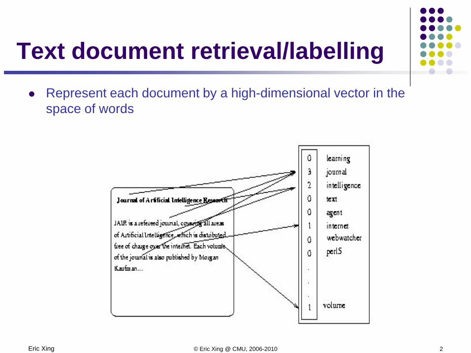
Text document retrieval/labelling Represent each document by a high-dimensional vector in the
space of words
Eric Xing © Eric Xing @ CMU, 2006-2010 3
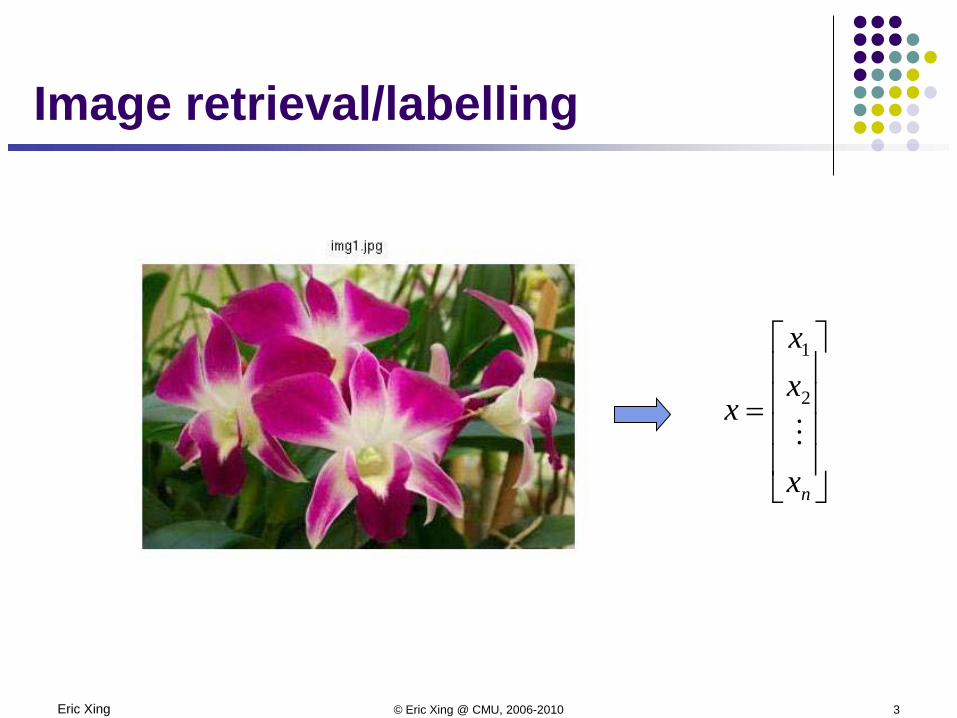
Image retrieval/labelling
=
nx
xx
x2
1
Eric Xing © Eric Xing @ CMU, 2006-2010 4
Dimensionality Bottlenecks
Data dimension Sensor response variables X:
1,000,000 samples of an EM/Acoustic field on each of N sensors 10242 pixels of a projected image on a IR camera sensor N2 expansion factor to account for all pairwise correlations
Information dimension Number of free parameters describing probability densities f(X) or f(S|X)
For known statistical model: info dim = model dim For unknown model: info dim = dim of density approximation
Parametric-model driven dimension reduction DR by sufficiency, DR by maximum likelihood
Data-driven dimension reduction Manifold learning, structure discovery
Eric Xing © Eric Xing @ CMU, 2006-2010 5
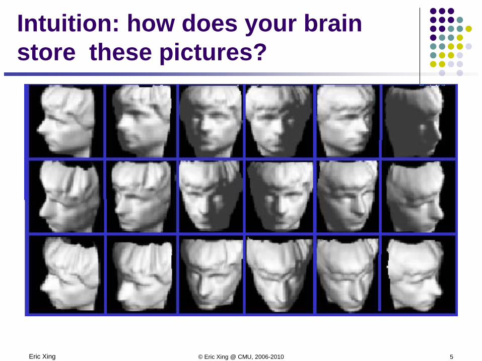
Intuition: how does your brain store these pictures?
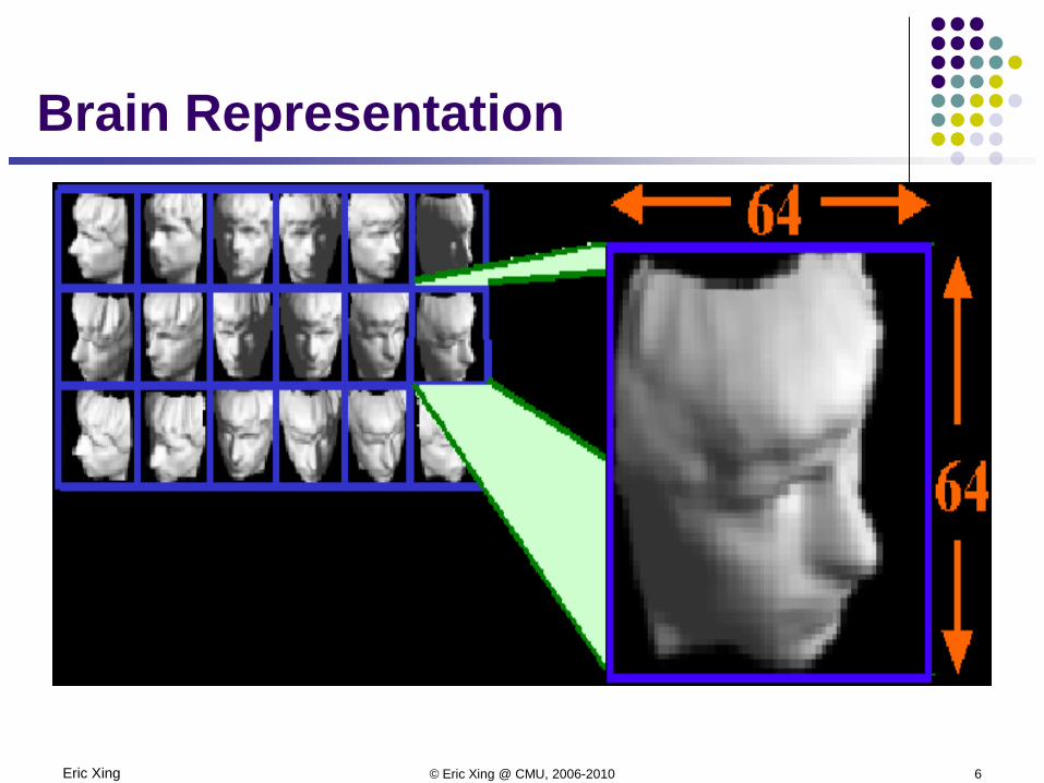
Eric Xing © Eric Xing @ CMU, 2006-2010 6
Brain Representation
Eric Xing © Eric Xing @ CMU, 2006-2010 7
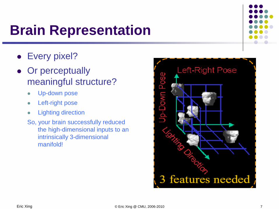
Brain Representation
Every pixel? Or perceptually
meaningful structure? Up-down pose Left-right pose Lighting directionSo, your brain successfully reduced
the high-dimensional inputs to an intrinsically 3-dimensional manifold!
Eric Xing © Eric Xing @ CMU, 2006-2010 8
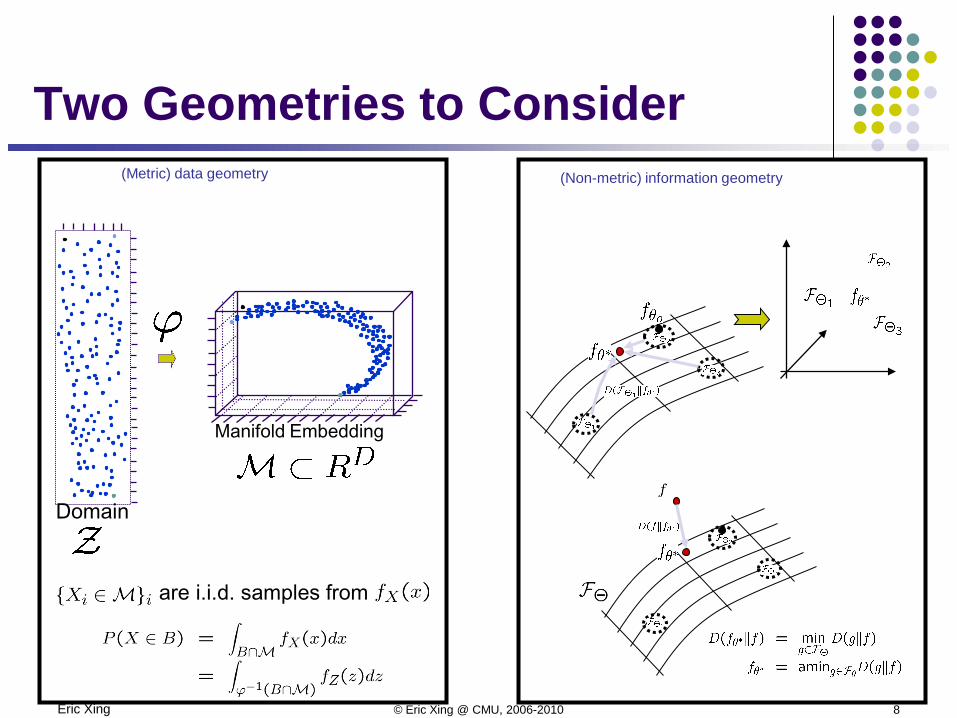
Manifold Embedding
(Metric) data geometry (Non-metric) information geometry
Domain
are i.i.d. samples from
Two Geometries to Consider
Eric Xing © Eric Xing @ CMU, 2006-2010 9
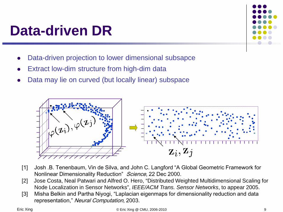
Data-driven projection to lower dimensional subsapce Extract low-dim structure from high-dim data Data may lie on curved (but locally linear) subspace
[1] Josh .B. Tenenbaum, Vin de Silva, and John C. Langford “A Global Geometric Framework for Nonlinear Dimensionality Reduction” Science, 22 Dec 2000.
[2] Jose Costa, Neal Patwari and Alfred O. Hero, “Distributed Weighted Multidimensional Scaling for Node Localization in Sensor Networks”, IEEE/ACM Trans. Sensor Networks, to appear 2005.
[3] Misha Belkin and Partha Niyogi, “Laplacian eigenmaps for dimensionality reduction and data representation,” Neural Computation, 2003.
Data-driven DR
Eric Xing © Eric Xing @ CMU, 2006-2010 10
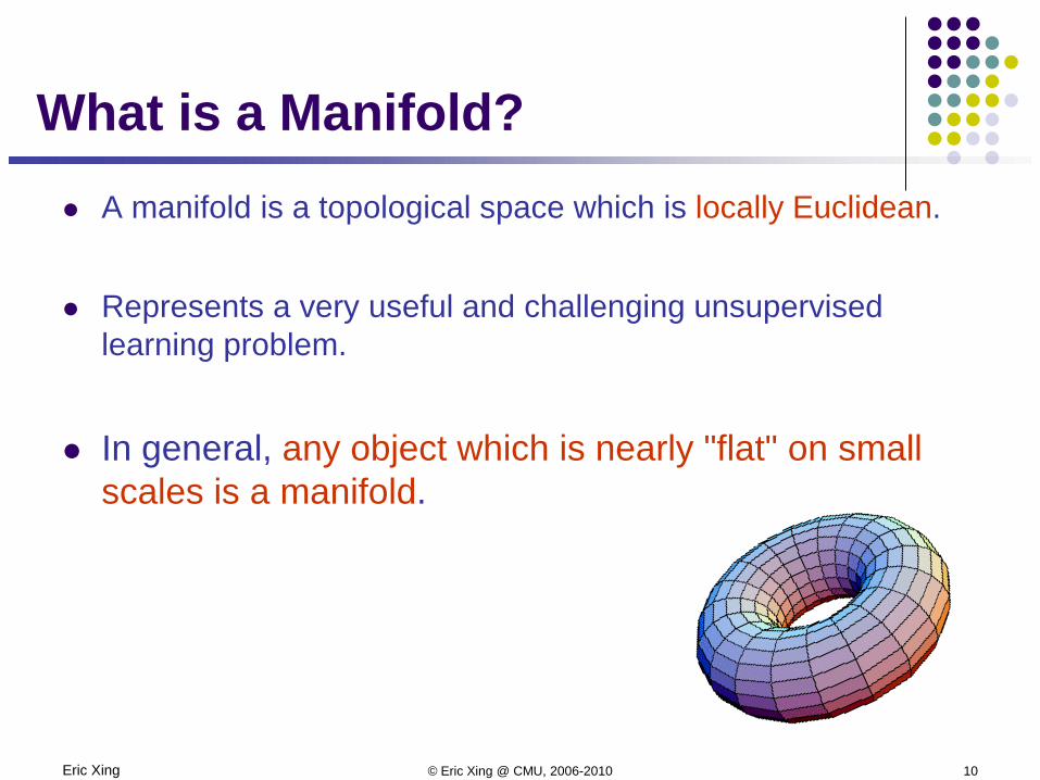
What is a Manifold? A manifold is a topological space which is locally Euclidean.
Represents a very useful and challenging unsupervised learning problem.
In general, any object which is nearly "flat" on small scales is a manifold.
Eric Xing © Eric Xing @ CMU, 2006-2010 11
Manifold Learning Discover low dimensional structures (smooth manifold) for
data in high dimension.
Linear Approaches Principal component analysis. Multi dimensional scaling.
Non Linear Approaches Local Linear Embedding ISOMAP Laplacian Eigenmap.
Eric Xing © Eric Xing @ CMU, 2006-2010 12
Principal component analysis Areas of variance in data are where items can be best discriminated
and key underlying phenomena observed
If two items or dimensions are highly correlated or dependent They are likely to represent highly related phenomena We want to combine related variables, and focus on uncorrelated or independent ones,
especially those along which the observations have high variance
We look for the phenomena underlying the observed covariance/co-dependence in a set of variables
These phenomena are called “factors” or “principal components” or “independent components,” depending on the methods used Factor analysis: based on variance/covariance/correlation Independent Component Analysis: based on independence
Eric Xing © Eric Xing @ CMU, 2006-2010 13
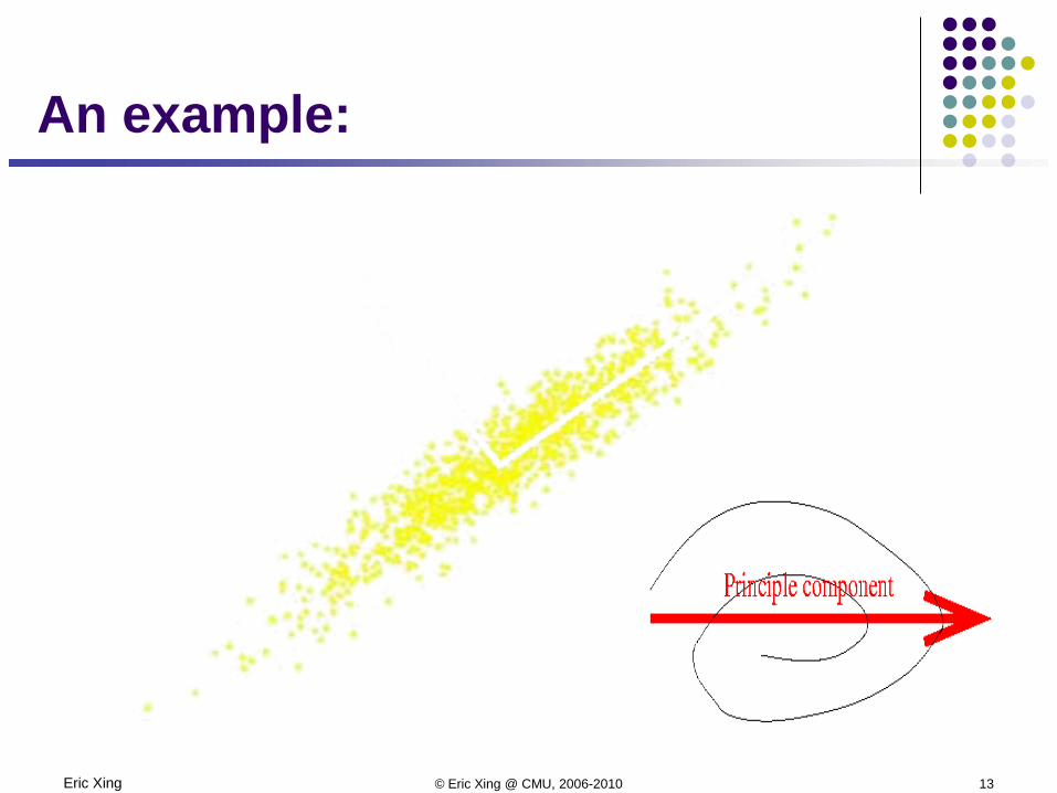
An example:
Eric Xing © Eric Xing @ CMU, 2006-2010 14
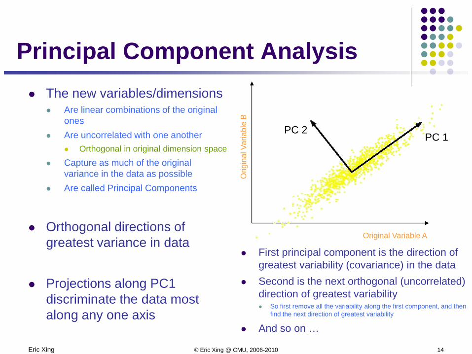
Principal Component Analysis The new variables/dimensions
Are linear combinations of the original ones
Are uncorrelated with one another Orthogonal in original dimension space
Capture as much of the original variance in the data as possible
Are called Principal Components
Orthogonal directions of greatest variance in data
Projections along PC1 discriminate the data most along any one axis
First principal component is the direction of greatest variability (covariance) in the data
Second is the next orthogonal (uncorrelated) direction of greatest variability So first remove all the variability along the first component, and then
find the next direction of greatest variability
And so on …
Original Variable AO
rigin
al V
aria
ble
B
PC 1PC 2
Eric Xing © Eric Xing @ CMU, 2006-2010 15
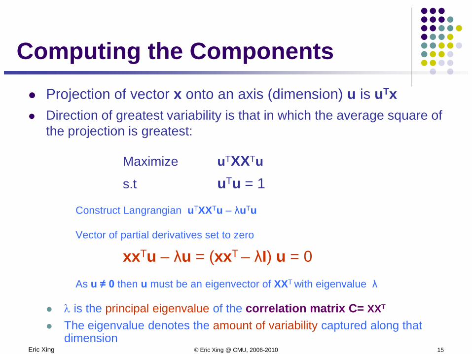
Computing the Components Projection of vector x onto an axis (dimension) u is uTx Direction of greatest variability is that in which the average square of
the projection is greatest:
Maximize uTXXTus.t uTu = 1
Construct Langrangian uTXXTu – λuTu
Vector of partial derivatives set to zero
xxTu – λu = (xxT – λI) u = 0As u ≠ 0 then u must be an eigenvector of XXT with eigenvalue λ
λ is the principal eigenvalue of the correlation matrix C= XXT
The eigenvalue denotes the amount of variability captured along that dimension
Eric Xing © Eric Xing @ CMU, 2006-2010 16
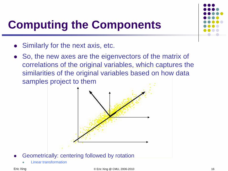
Computing the Components Similarly for the next axis, etc. So, the new axes are the eigenvectors of the matrix of
correlations of the original variables, which captures the similarities of the original variables based on how data samples project to them
Geometrically: centering followed by rotation Linear transformation
Eric Xing © Eric Xing @ CMU, 2006-2010 17
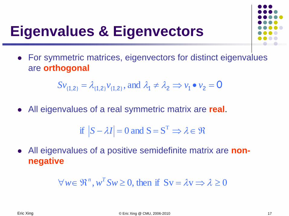
For symmetric matrices, eigenvectors for distinct eigenvalues are orthogonal
All eigenvalues of a real symmetric matrix are real.
All eigenvalues of a positive semidefinite matrix are non-negative
ℜ∈⇒==− λλ TSS and 0 if IS
0vSv if then ,0, ≥⇒=≥ℜ∈∀ λλSwww Tn
02121212121 =•⇒≠= vvvSv λλλ and ,},{},{},{
Eigenvalues & Eigenvectors
Eric Xing © Eric Xing @ CMU, 2006-2010 18
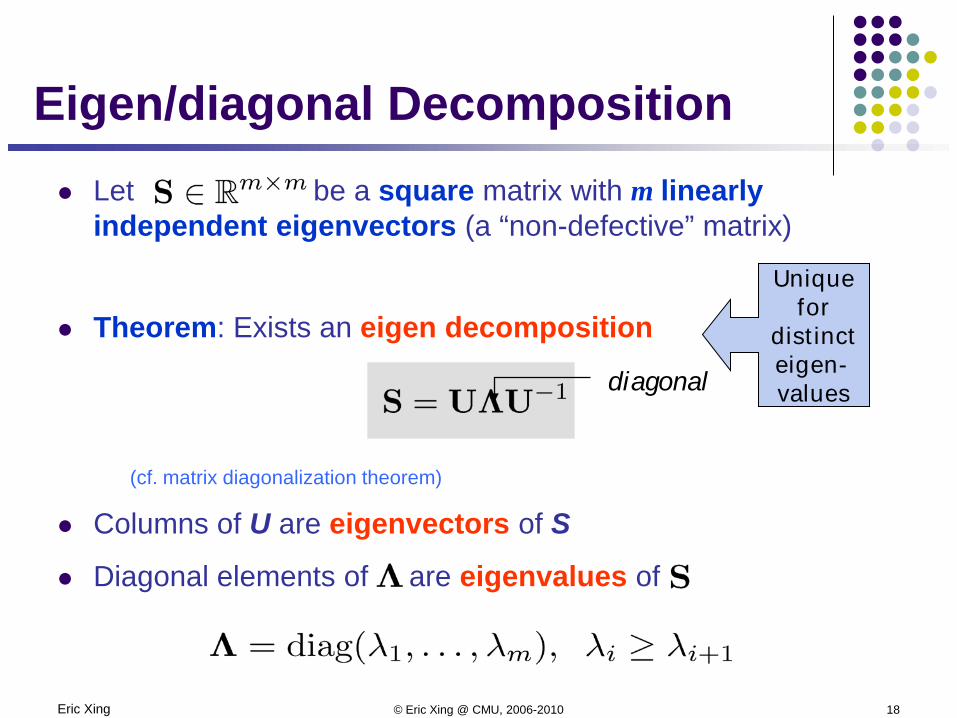
Let be a square matrix with m linearly independent eigenvectors (a “non-defective” matrix)
Theorem: Exists an eigen decomposition
(cf. matrix diagonalization theorem)
Columns of U are eigenvectors of S
Diagonal elements of are eigenvalues of
Eigen/diagonal Decomposition
diagonal
Unique for
distinct eigen-values
Eric Xing © Eric Xing @ CMU, 2006-2010 19
PCs, Variance and Least-Squares The first PC retains the greatest amount of variation in the
sample
The kth PC retains the kth greatest fraction of the variation in the sample
The kth largest eigenvalue of the correlation matrix C is the variance in the sample along the kth PC
The least-squares view: PCs are a series of linear least squares fits to a sample, each orthogonal to all previous ones
Eric Xing © Eric Xing @ CMU, 2006-2010 20
0
5
10
15
20
25
PC1 PC2 PC3 PC4 PC5 PC6 PC7 PC8 PC9 PC10
Varia
nce
(%)
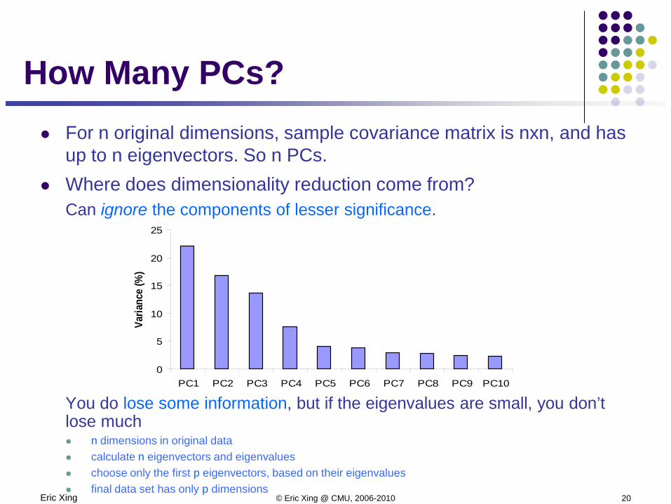
How Many PCs? For n original dimensions, sample covariance matrix is nxn, and has
up to n eigenvectors. So n PCs. Where does dimensionality reduction come from?
Can ignore the components of lesser significance.
You do lose some information, but if the eigenvalues are small, you don’t lose much n dimensions in original data calculate n eigenvectors and eigenvalues choose only the first p eigenvectors, based on their eigenvalues final data set has only p dimensions
Eric Xing © Eric Xing @ CMU, 2006-2010 21
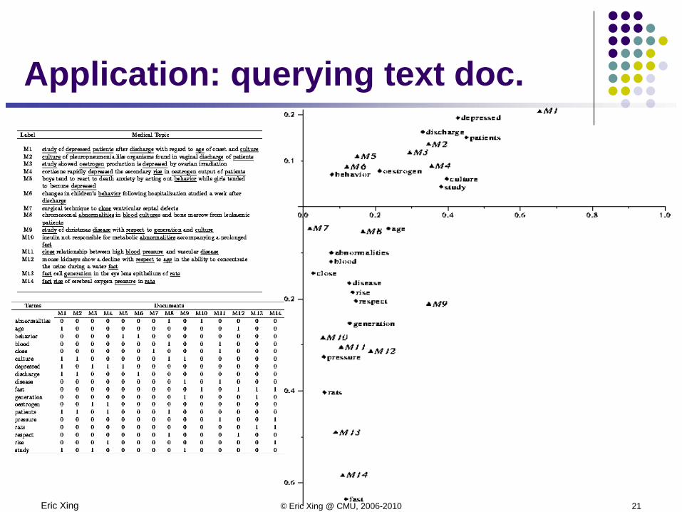
Application: querying text doc.
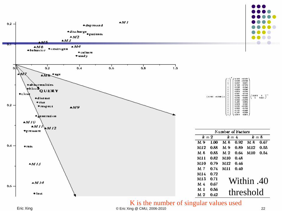
Eric Xing © Eric Xing @ CMU, 2006-2010 22
Within .40threshold
K is the number of singular values used
Eric Xing © Eric Xing @ CMU, 2006-2010 23
Summary: Principle
Linear projection method to reduce the number of parameters Transfer a set of correlated variables into a new set of uncorrelated variables Map the data into a space of lower dimensionality Form of unsupervised learning
Properties It can be viewed as a rotation of the existing axes to new positions in the space defined by
original variables New axes are orthogonal and represent the directions with maximum variability
Application: In many settings in pattern recognition and retrieval, we have a feature-object matrix. For text, the terms are features and the docs are objects. Could be opinions and users … This matrix may be redundant in dimensionality. Can work with low-rank approximation. If entries are missing (e.g., users’ opinions), can recover if dimensionality is low.
Eric Xing © Eric Xing @ CMU, 2006-2010 24
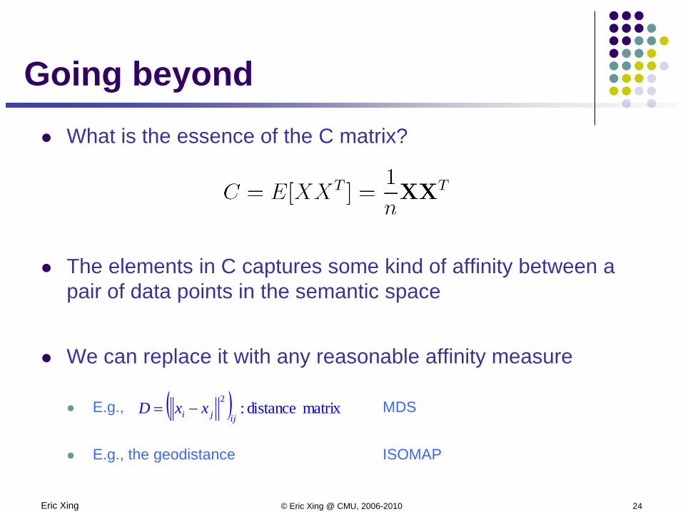
Going beyond What is the essence of the C matrix?
The elements in C captures some kind of affinity between a pair of data points in the semantic space
We can replace it with any reasonable affinity measure
E.g., MDS
E.g., the geodistance ISOMAP
( ) matrix distance:2
ijji xxD −=
Eric Xing © Eric Xing @ CMU, 2006-2010 25
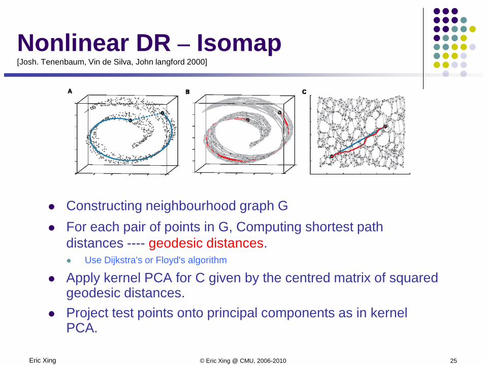
Constructing neighbourhood graph G For each pair of points in G, Computing shortest path
distances ---- geodesic distances. Use Dijkstra's or Floyd's algorithm
Apply kernel PCA for C given by the centred matrix of squared geodesic distances.
Project test points onto principal components as in kernel PCA.
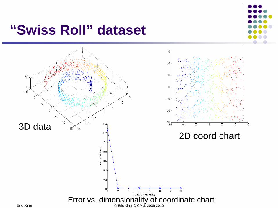
Nonlinear DR – Isomap[Josh. Tenenbaum, Vin de Silva, John langford 2000]
Eric Xing © Eric Xing @ CMU, 2006-2010
3D data2D coord chart
Error vs. dimensionality of coordinate chart
“Swiss Roll” dataset
Eric Xing © Eric Xing @ CMU, 2006-2010 27
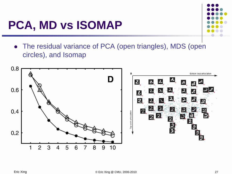
PCA, MD vs ISOMAP The residual variance of PCA (open triangles), MDS (open
circles), and Isomap
Eric Xing © Eric Xing @ CMU, 2006-2010 28
ISOMAP algorithm Pros/Cons
Advantages: Nonlinear Globally optimal Guarantee asymptotically to recover the true
dimensionality
Drawback: May not be stable, dependent on topology of data As N increases, pair wise distances provide better
approximations to geodesics, but cost more computation
Eric Xing © Eric Xing @ CMU, 2006-2010 29
Local Linear Embedding (a.k.a LLE)
LLE is based on simple geometric intuitions.
Suppose the data consist of N real-valuedvectors Xi, each of dimensionality D.
Each data point and its neighbors expected to lie on or close to a locally linear patch of the manifold.
Eric Xing © Eric Xing @ CMU, 2006-2010 30
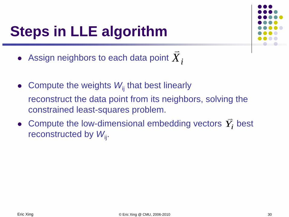
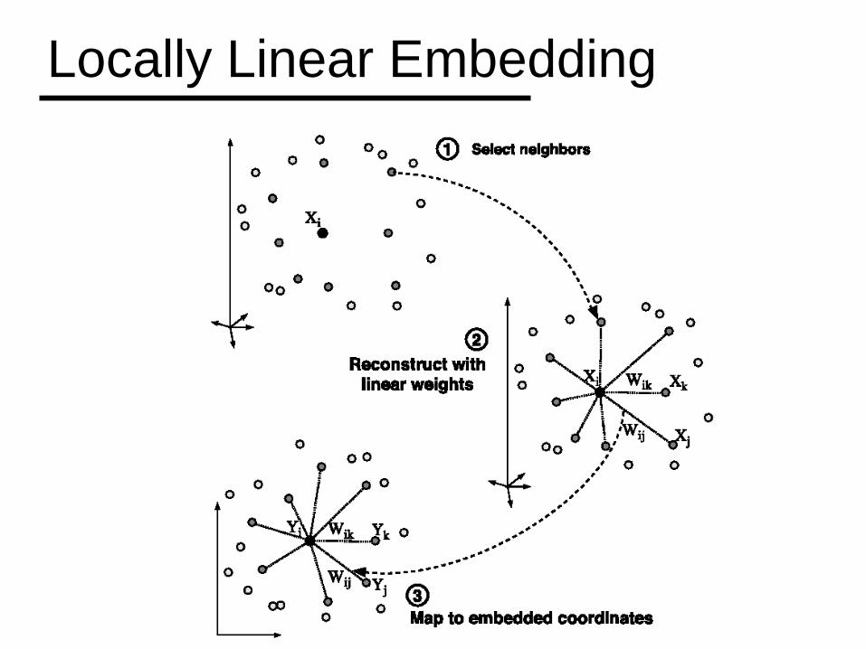
Steps in LLE algorithm Assign neighbors to each data point
Compute the weights Wij that best linearlyreconstruct the data point from its neighbors, solving the constrained least-squares problem.
Compute the low-dimensional embedding vectors best reconstructed by Wij.
iX
iY
Eric Xing © Eric Xing @ CMU, 2006-2010 31
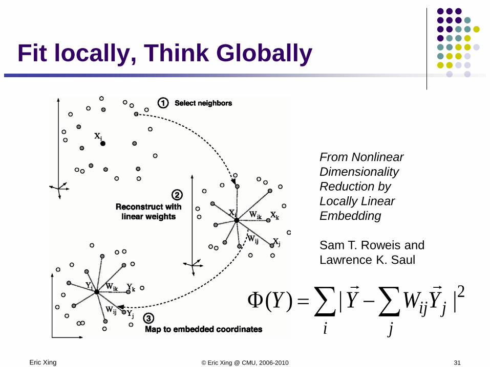
Fit locally, Think Globally
From Nonlinear DimensionalityReduction byLocally Linear Embedding
Sam T. Roweis and Lawrence K. Saul
∑ ∑−=Φi j
jijYWYY 2||)(
Eric Xing © Eric Xing @ CMU, 2006-2010 32
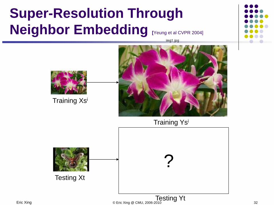
Super-Resolution Through Neighbor Embedding [Yeung et al CVPR 2004]
Training Xsi
Training Ysi
Testing Xt
Testing Yt
?
Eric Xing © Eric Xing @ CMU, 2006-2010 33
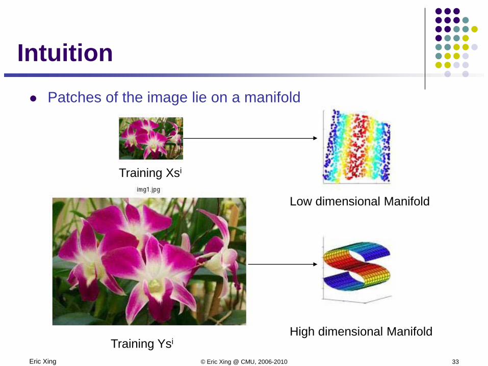
Training Xsi
Training YsiHigh dimensional Manifold
Low dimensional Manifold
Intuition Patches of the image lie on a manifold
Eric Xing © Eric Xing @ CMU, 2006-2010 34
Algorithm
1. Get feature vectors for each low resolution training patch.
2. For each test patch feature vector find K nearest neighboring feature vectors of training patches.
3. Find optimum weights to express each test patch vector as a weighted sum of its K nearest neighbor vectors.
4. Use these weights for reconstruction of that test patch in high resolution.
Eric Xing © Eric Xing @ CMU, 2006-2010 35
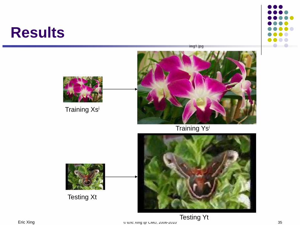
Training Xsi
Training Ysi
Testing Xt
Testing Yt
Results
Eric Xing © Eric Xing @ CMU, 2006-2010 36
Summary: Principle
Linear and nonlinear projection method to reduce the number of parameters Transfer a set of correlated variables into a new set of uncorrelated variables Map the data into a space of lower dimensionality Form of unsupervised learning
Applications PCA and Latent semantic indexing for text mining Isomap and Nonparametric Models of Image Deformation LLE and Isomap Analysis of Spectra and Colour Images Image Spaces and Video Trajectories: Using Isomap to Explore Video Sequences Mining the structural knowledge of high-dimensional medical data using isomap
Isomap Webpage: http://isomap.stanford.edu/
Applying PCA and LDA:Eigen-faces and Fisher-faces
L. Fei-Fei
Computer Science Dept.
Stanford University
Machine learning in computer vision
• Aug 13, Lecture 7: Dimensionality reduction, Manifold learning– Eigen- and Fisher- faces
– Applications to object representation
8/8/2010 38L. Fei-Fei, Dragon Star 2010, Stanford
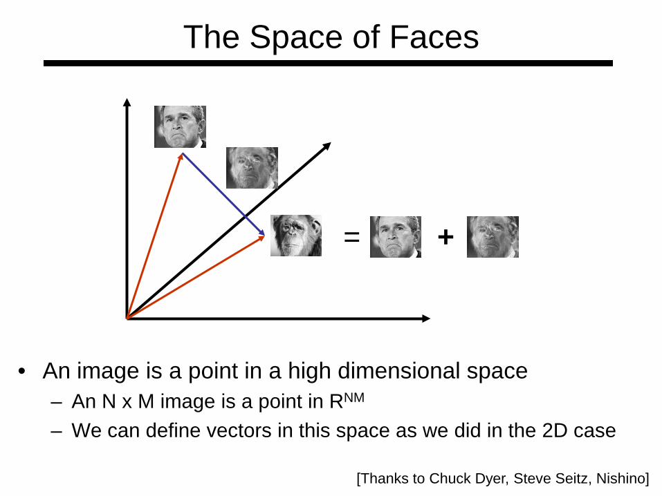
The Space of Faces
• An image is a point in a high dimensional space– An N x M image is a point in RNM
– We can define vectors in this space as we did in the 2D case
+=
[Thanks to Chuck Dyer, Steve Seitz, Nishino]
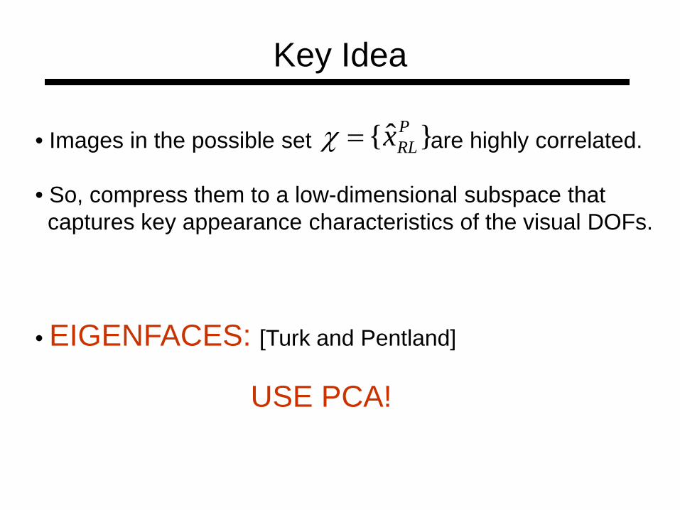
Key Idea
}ˆ{ PRLx=χ• Images in the possible set are highly correlated.
• So, compress them to a low-dimensional subspace thatcaptures key appearance characteristics of the visual DOFs.
• EIGENFACES: [Turk and Pentland]
USE PCA!
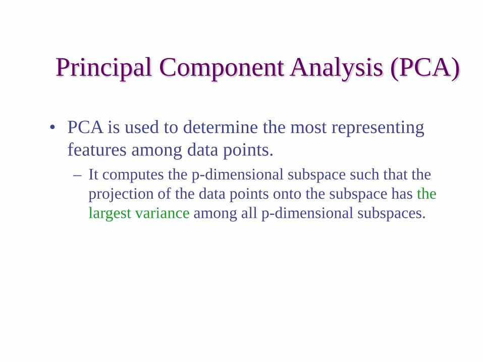
Principal Component Analysis (PCA)
• PCA is used to determine the most representing features among data points. – It computes the p-dimensional subspace such that the
projection of the data points onto the subspace has the largest variance among all p-dimensional subspaces.
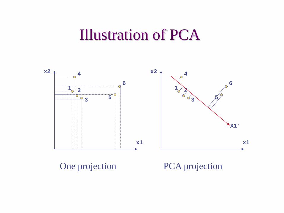
Illustration of PCA
One projection PCA projection
x1
x2
1 2
3
4
5
6
x1
x2
1 2
3
4
5
6
X1’
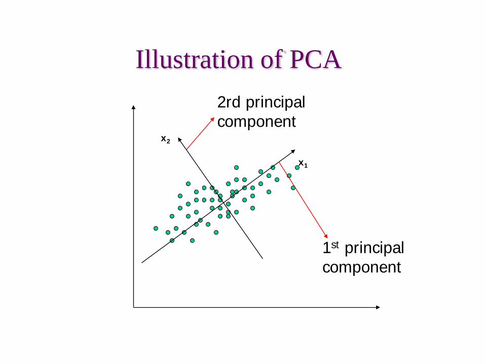
Illustration of PCA
x1
x2
1st principal component
2rd principal component
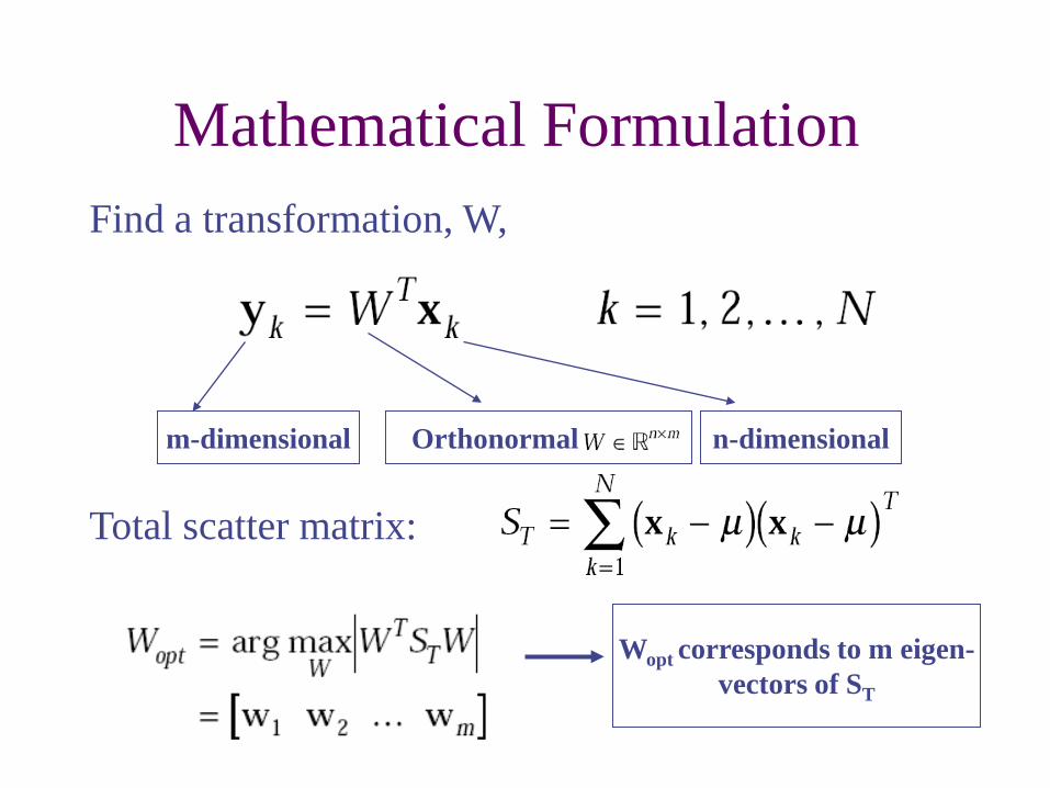
Mathematical FormulationFind a transformation, W,
m-dimensional n-dimensionalOrthonormal
Total scatter matrix:
Wopt corresponds to m eigen-vectors of ST
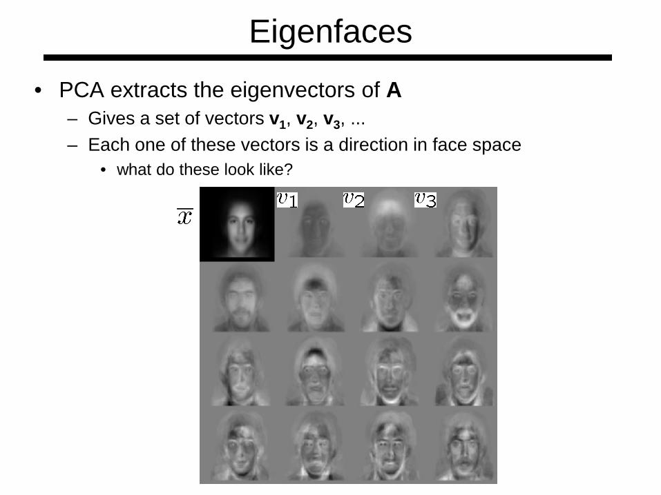
Eigenfaces• PCA extracts the eigenvectors of A
– Gives a set of vectors v1, v2, v3, ...– Each one of these vectors is a direction in face space
• what do these look like?
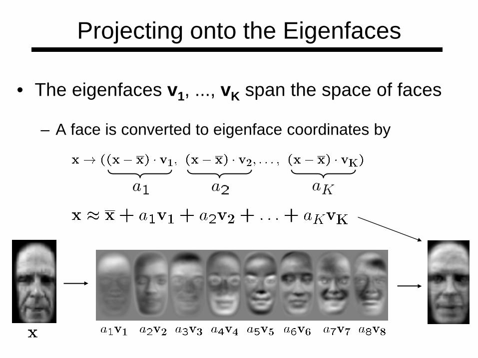
Projecting onto the Eigenfaces
• The eigenfaces v1, ..., vK span the space of faces
– A face is converted to eigenface coordinates by
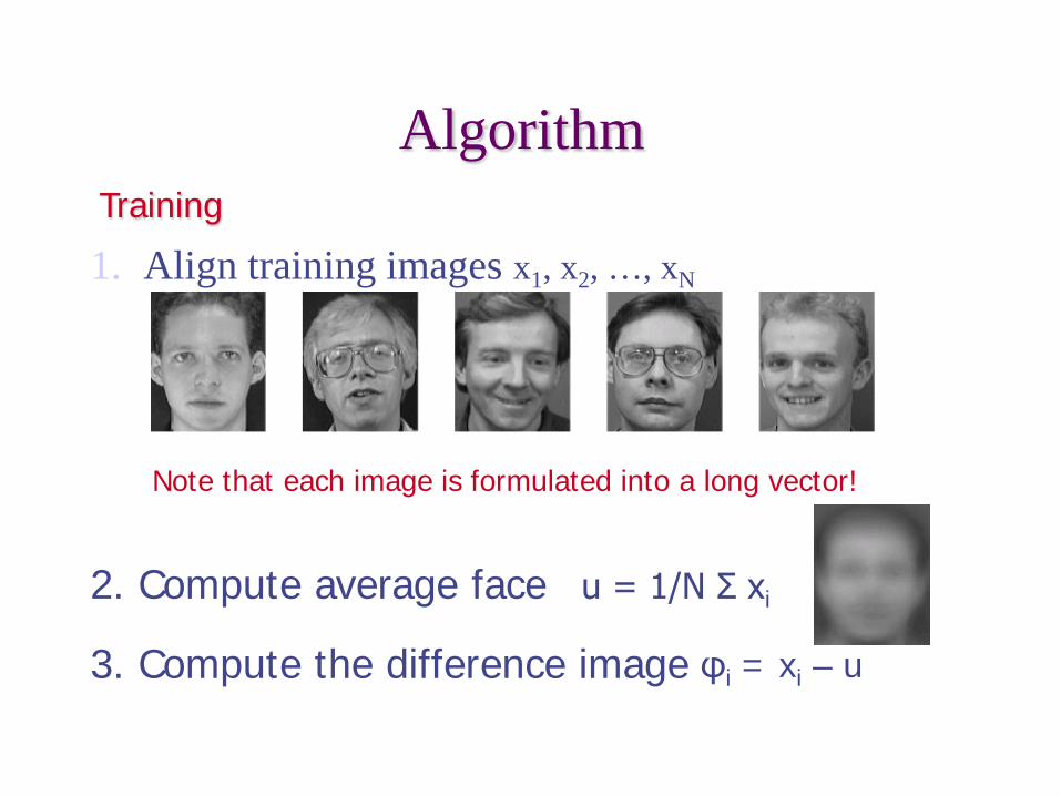
Algorithm
1. Align training images x1, x2, …, xN
2. Compute average face u = 1/N Σ xi
3. Compute the difference image φi = xi – u
Training
Note that each image is formulated into a long vector!
Algorithm
Testing 1. Projection in Eigenface
Projection ωi = W (X – u), W = {eigenfaces}
2. Compare projections
ST = 1/NΣ φi φiT = BBT, B=[φ1, φ2 … φN]
4. Compute the covariance matrix (total scatter matrix)
5. Compute the eigenvectors of the covariance matrix , W
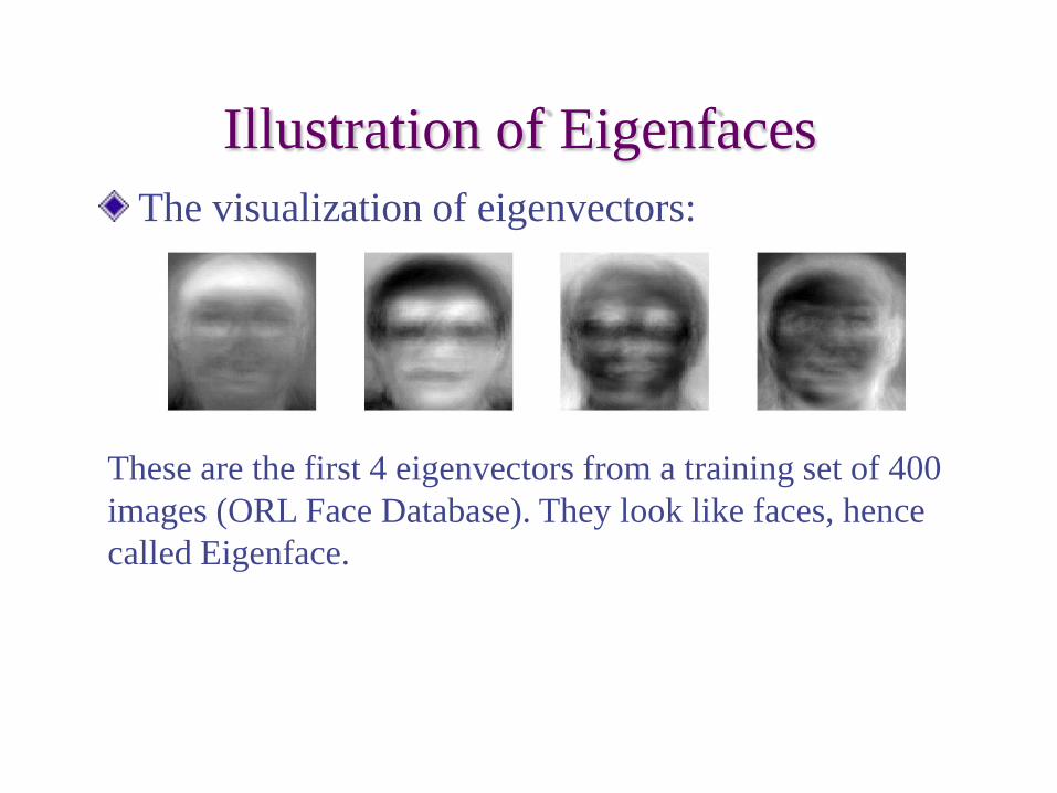
Illustration of Eigenfaces
These are the first 4 eigenvectors from a training set of 400 images (ORL Face Database). They look like faces, hence called Eigenface.
The visualization of eigenvectors:
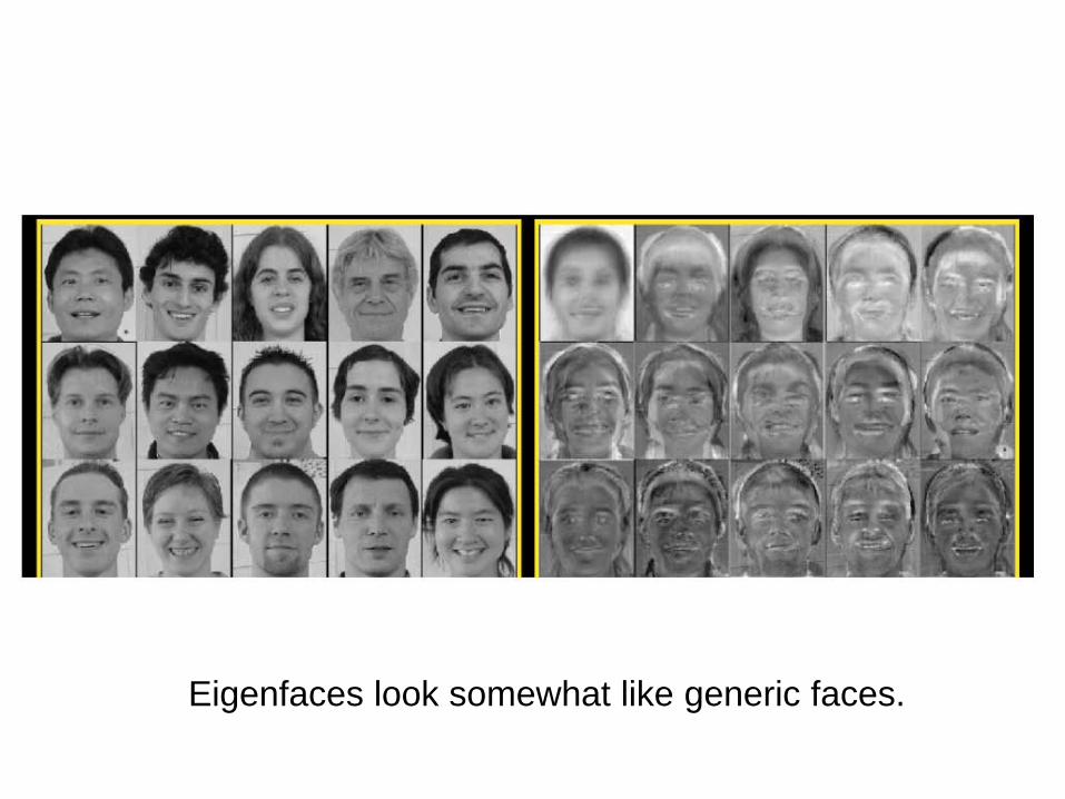
Eigenfaces look somewhat like generic faces.
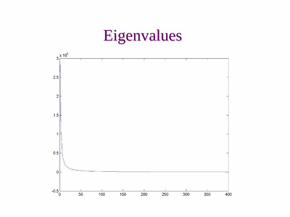
Eigenvalues
Only selecting the top P eigenfaces reduces the dimensionality.Fewer eigenfaces result in more information loss, and hence less discrimination between faces.
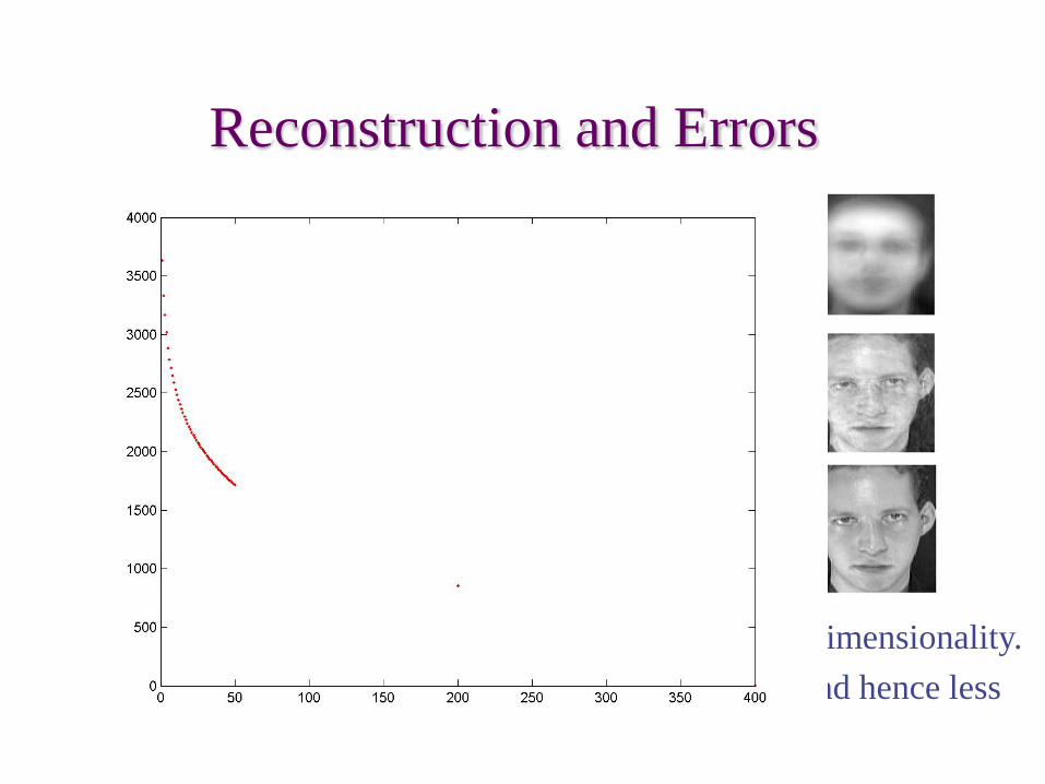
Reconstruction and Errors
P = 4
P = 200
P = 400
Summary for PCA and Eigenface• Non-iterative, globally optimal solution• PCA projection is optimal for reconstruction
from a low dimensional basis, but may NOT be optimal for discrimination…
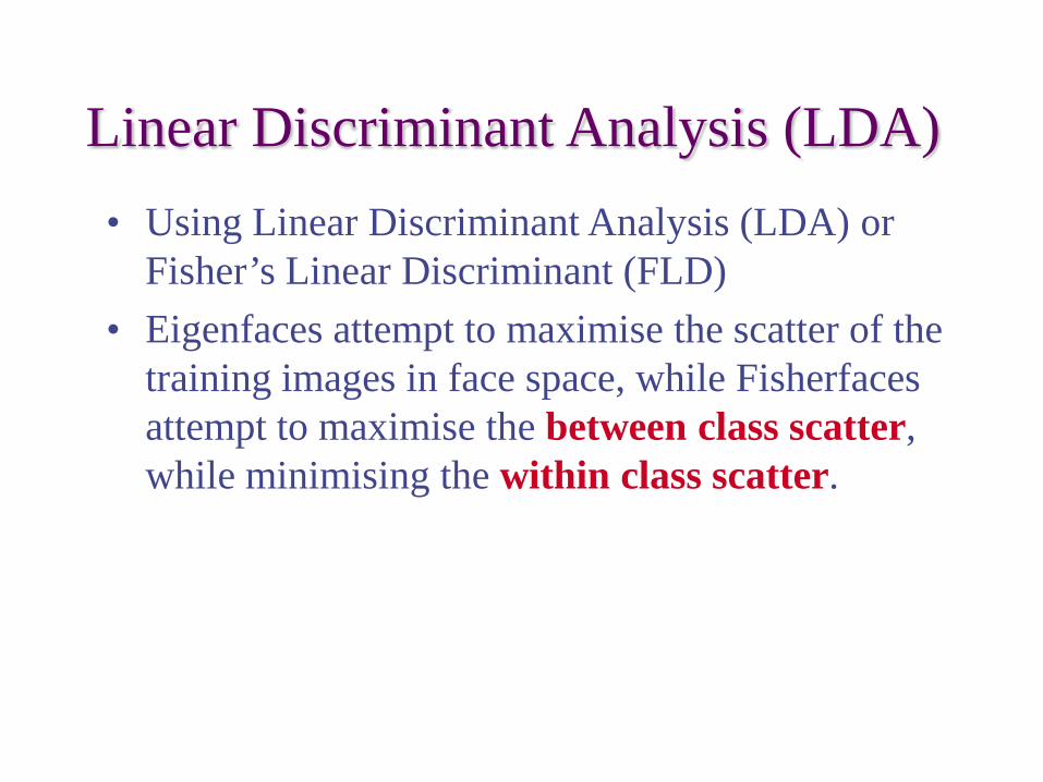
Linear Discriminant Analysis (LDA)• Using Linear Discriminant Analysis (LDA) or
Fisher’s Linear Discriminant (FLD) • Eigenfaces attempt to maximise the scatter of the
training images in face space, while Fisherfacesattempt to maximise the between class scatter, while minimising the within class scatter.
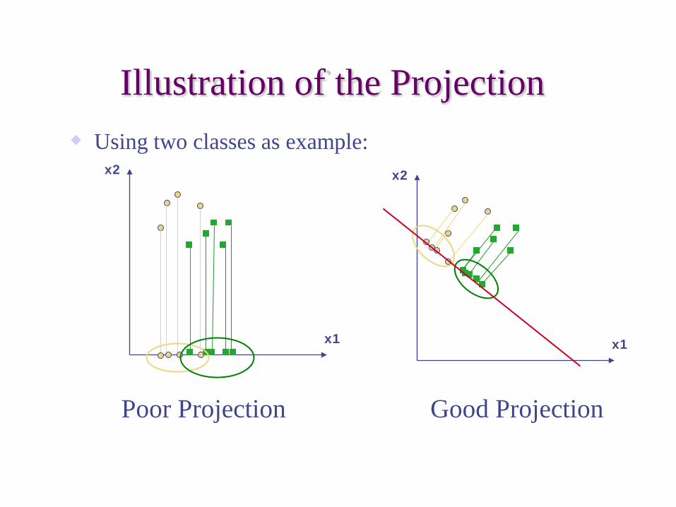
Illustration of the Projection
Poor Projection Good Projection
x1
x2
x1
x2
Using two classes as example:
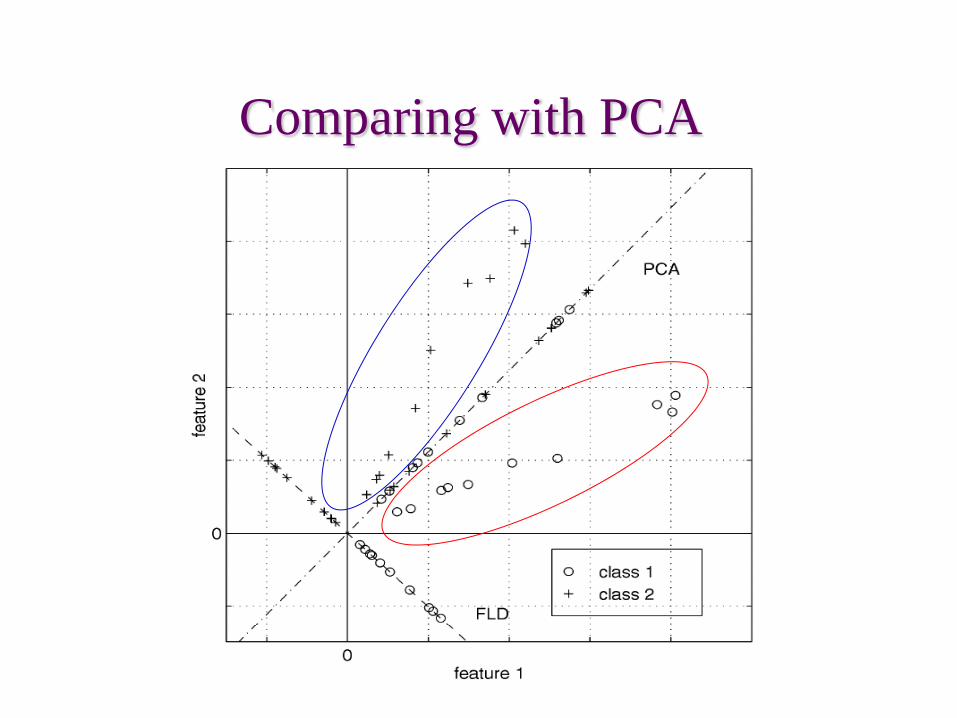
Comparing with PCA
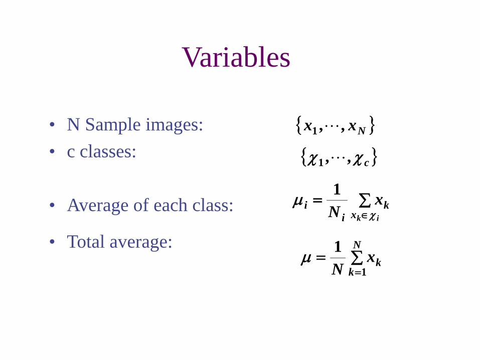
Variables
• N Sample images: • c classes:
• Average of each class:
• Total average:
{ }Nxx ,,1
{ }cχχ ,,1
∑=∈ ikx
ki
i xN χ
µ 1
∑==
N
kkx
N 1
1µ
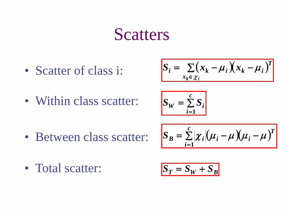
Scatters
• Scatter of class i: ( )( )Tikx
iki xxSik
µµχ
−∑ −=∈
∑==
c
iiW SS
1
( )( )∑ −−==
c
i
TiiiBS
1µµµµχ
BWT SSS +=
• Within class scatter:
• Between class scatter:
• Total scatter:
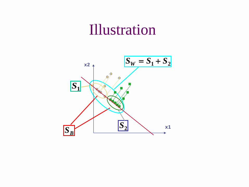
Illustration
2S
1S
BS
21 SSSW +=
x1
x2
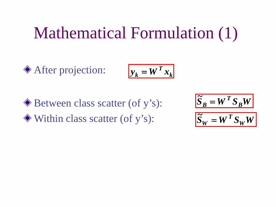
Mathematical Formulation (1)
After projection:
Between class scatter (of y’s):Within class scatter (of y’s):
kT
k xWy =
WSWS BT
B =~
WSWS WT
W =~
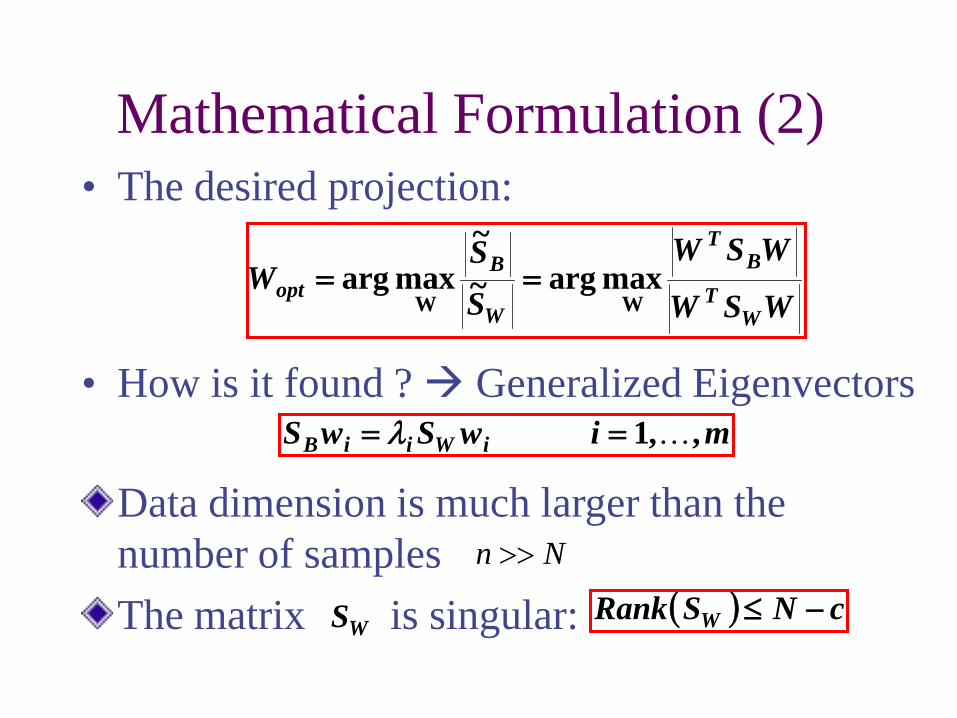
Mathematical Formulation (2)• The desired projection:
WSW
WSW
SS
WW
TB
T
W
Bopt WW
max arg~~
max arg ==
miwSwS iWiiB ,,1 == λ• How is it found ? Generalized Eigenvectors
Data dimension is much larger than the number of samplesThe matrix is singular:
Nn >>
( ) cNSRank W −≤WS
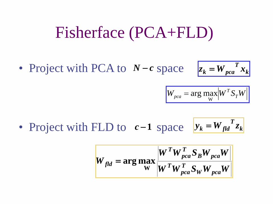
Fisherface (PCA+FLD)
• Project with FLD to space
• Project with PCA to space
1−c kT
fldk zWy =
WWSWW
WWSWWW
pcaWTpca
TpcaB
Tpca
T
fld Wmax arg=
cN − kT
pcak xWz =
WSWW TT
pca Wmax arg=
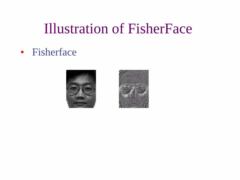
Illustration of FisherFace• Fisherface
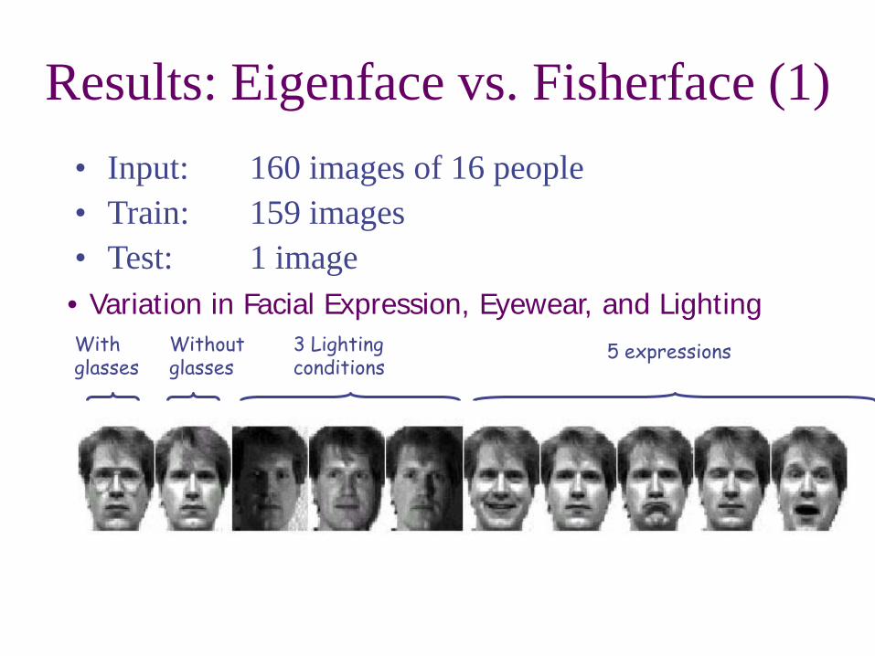
Results: Eigenface vs. Fisherface (1)
• Variation in Facial Expression, Eyewear, and Lighting
• Input: 160 images of 16 people• Train: 159 images• Test: 1 image
With glasses
Without glasses
3 Lighting conditions
5 expressions
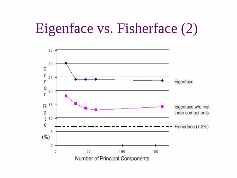
Eigenface vs. Fisherface (2)
discussion• Removing the first three principal
components results in better performance under variable lighting conditions
• The Firsherface methods had error rates lower than the Eigenface method for the small datasets tested.
Manifold Learning for Object Representation
L. Fei-Fei
Computer Science Dept.
Stanford University
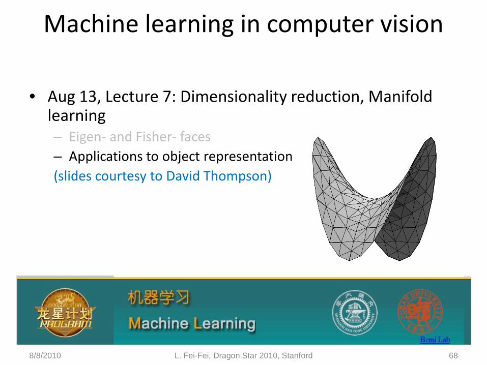
Machine learning in computer vision
• Aug 13, Lecture 7: Dimensionality reduction, Manifold learning– Eigen- and Fisher- faces– Applications to object representation(slides courtesy to David Thompson)
8/8/2010 68L. Fei-Fei, Dragon Star 2010, Stanford
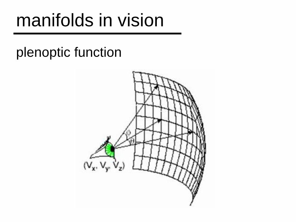
plenoptic function
manifolds in vision
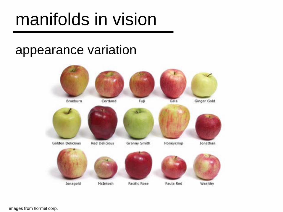
appearance variation
manifolds in vision
images from hormel corp.
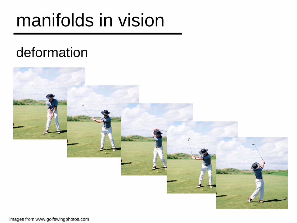
deformation
manifolds in vision
images from www.golfswingphotos.com
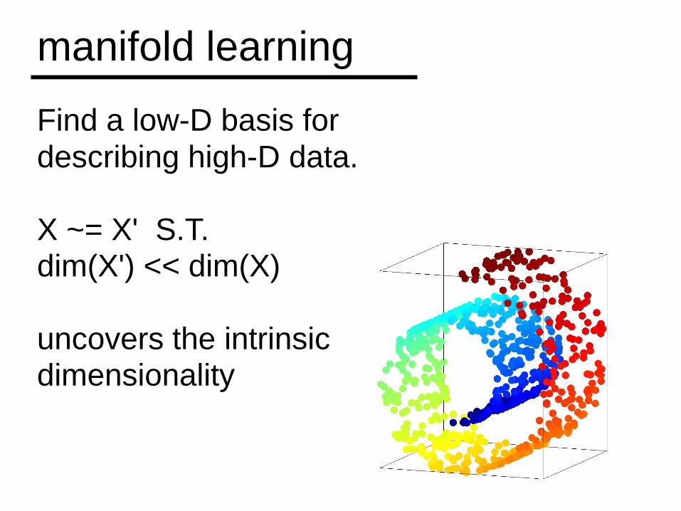
Find a low-D basis for describing high-D data.
X ~= X' S.T. dim(X') << dim(X)
uncovers the intrinsic dimensionality
manifold learning
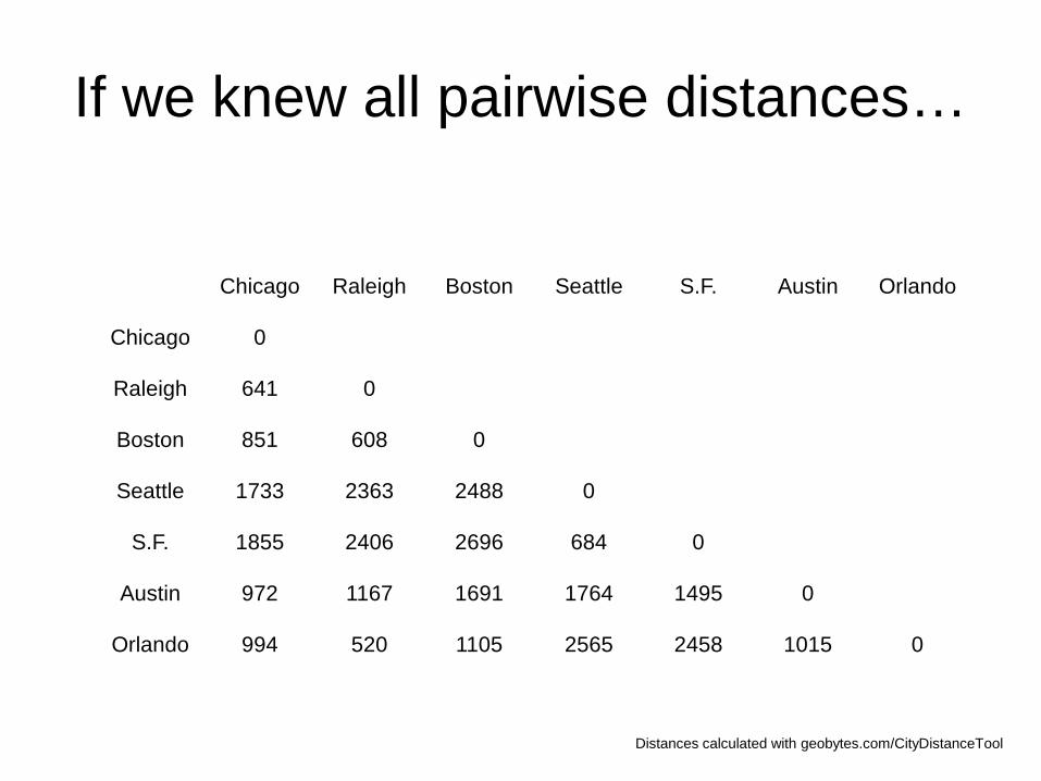
If we knew all pairwise distances…
Chicago Raleigh Boston Seattle S.F. Austin Orlando
Chicago 0
Raleigh 641 0
Boston 851 608 0
Seattle 1733 2363 2488 0
S.F. 1855 2406 2696 684 0
Austin 972 1167 1691 1764 1495 0
Orlando 994 520 1105 2565 2458 1015 0
Distances calculated with geobytes.com/CityDistanceTool
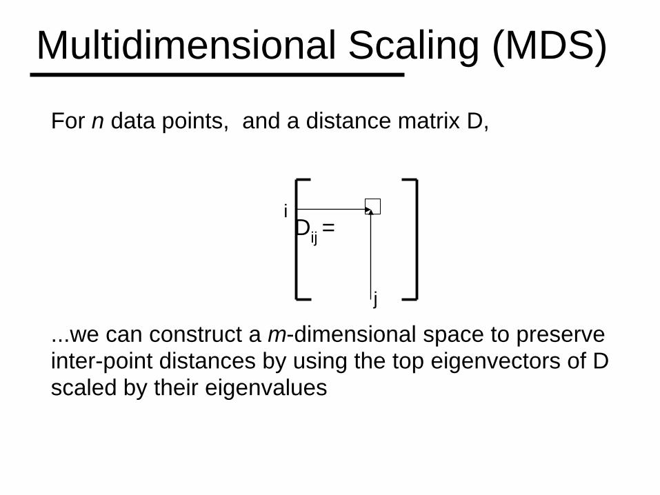
Multidimensional Scaling (MDS)
For n data points, and a distance matrix D,
Dij =
...we can construct a m-dimensional space to preserve inter-point distances by using the top eigenvectors of D scaled by their eigenvalues
j
i
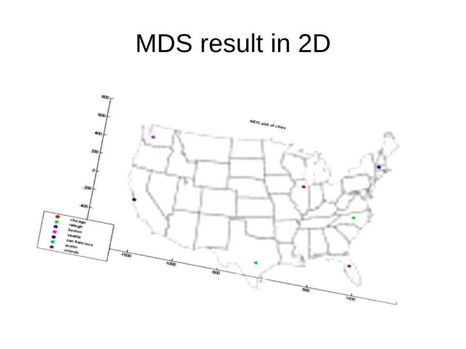
MDS result in 2D
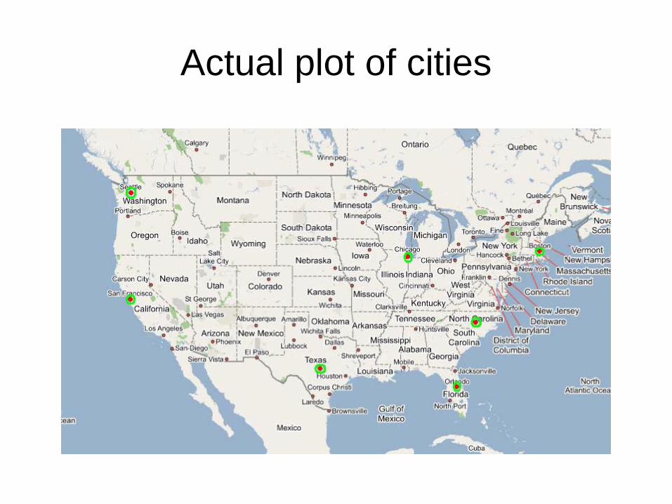
Actual plot of cities
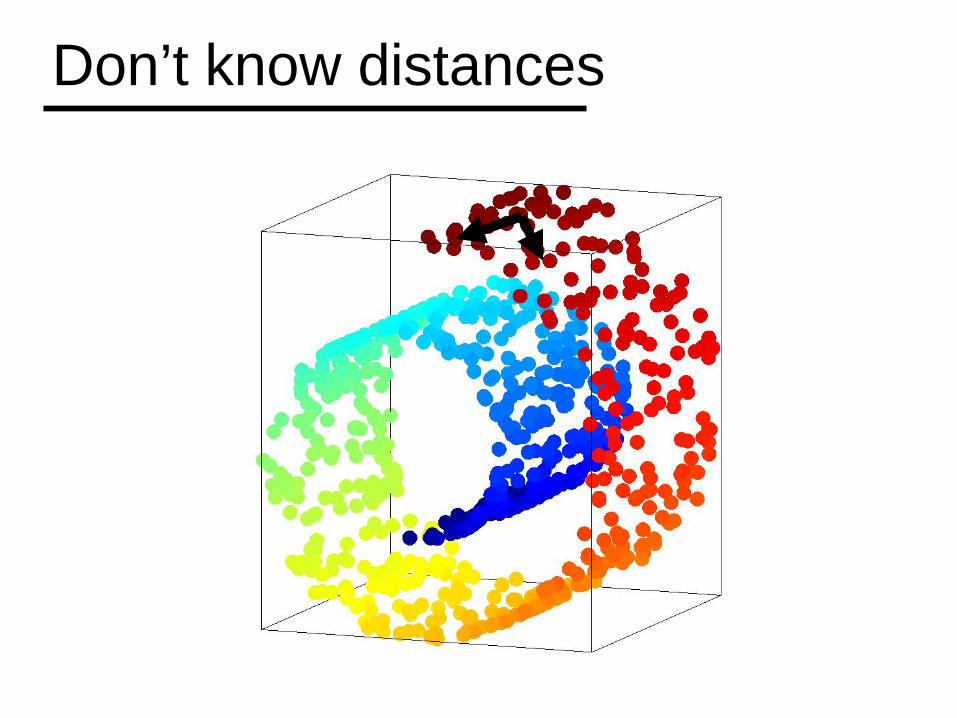
Don’t know distances
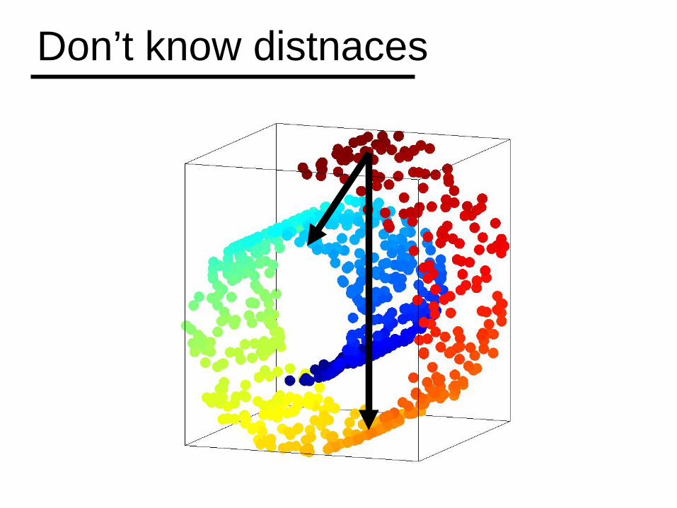
Don’t know distnaces
1. data compression
2. “curse of dimensionality”
3. de-noising
4. visualization
5. reasonable distance metrics
why do manifold learning?
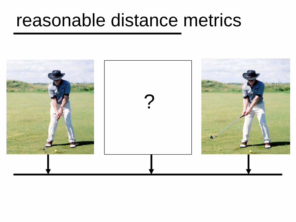
reasonable distance metrics
?
reasonable distance metrics
?
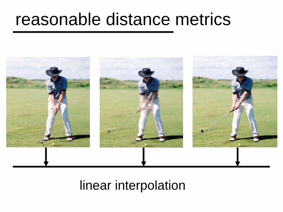
linear interpolation
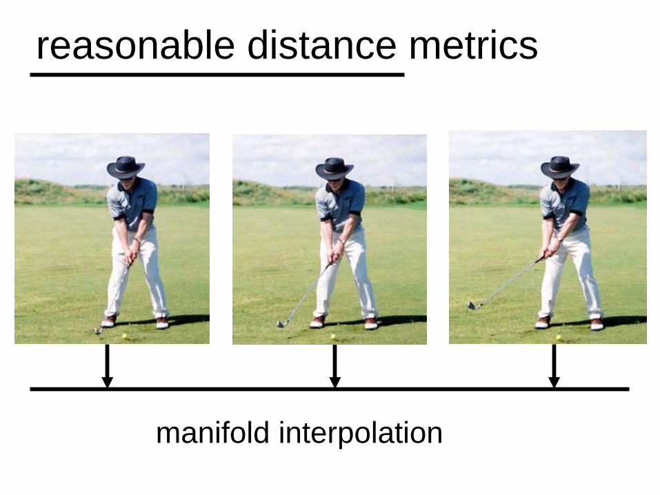
reasonable distance metrics
?
manifold interpolation
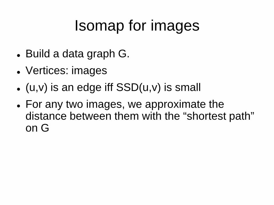
Isomap for images
Build a data graph G. Vertices: images (u,v) is an edge iff SSD(u,v) is small For any two images, we approximate the
distance between them with the “shortest path” on G
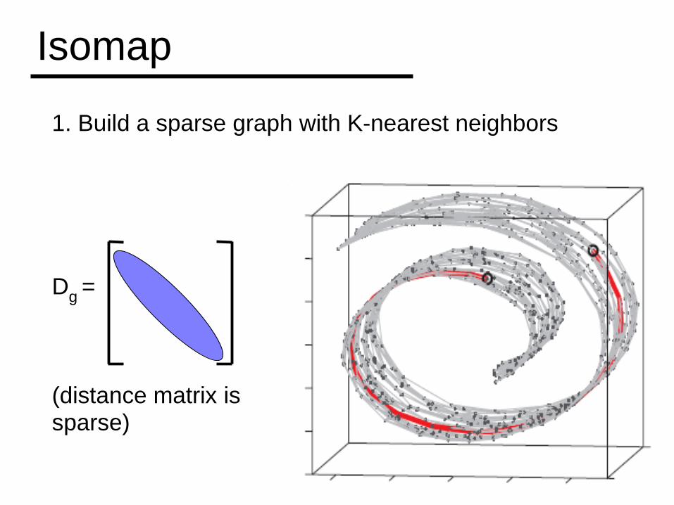
Isomap
1. Build a sparse graph with K-nearest neighbors
Dg =
(distance matrix issparse)
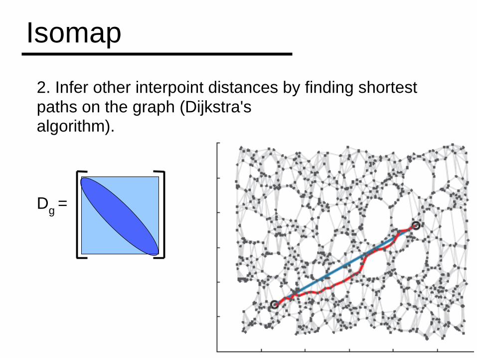
Isomap
2. Infer other interpoint distances by finding shortest paths on the graph (Dijkstra'salgorithm).
Dg =
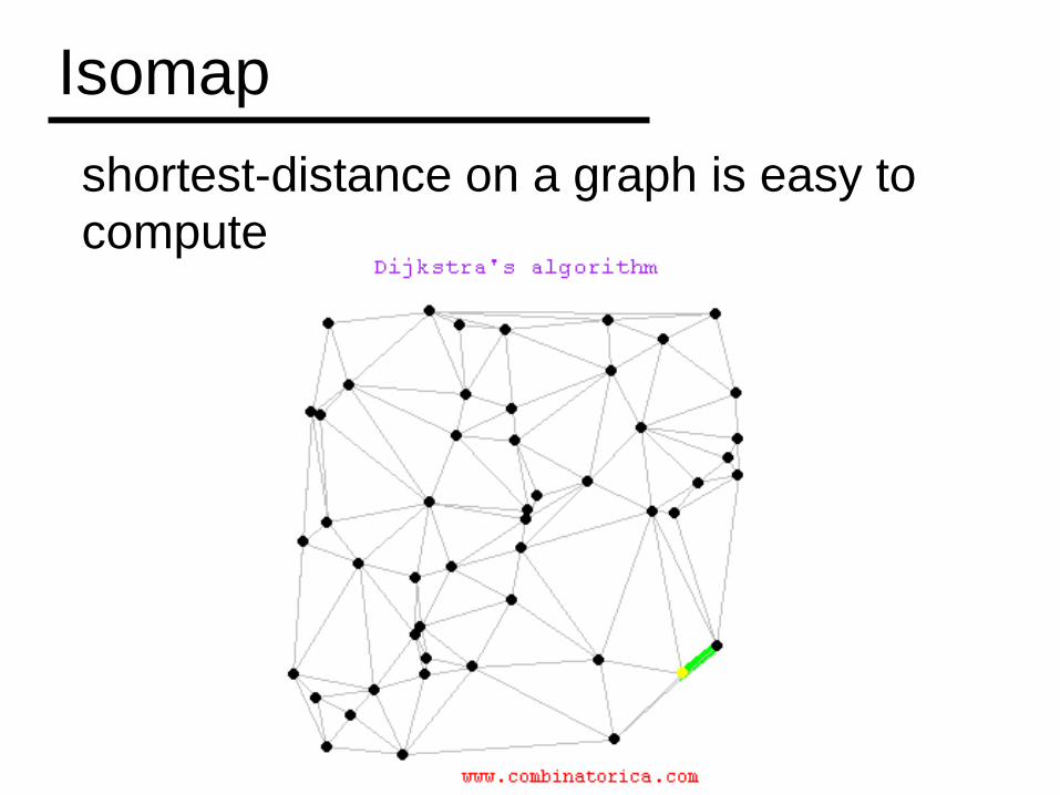
Isomapshortest-distance on a graph is easy to compute
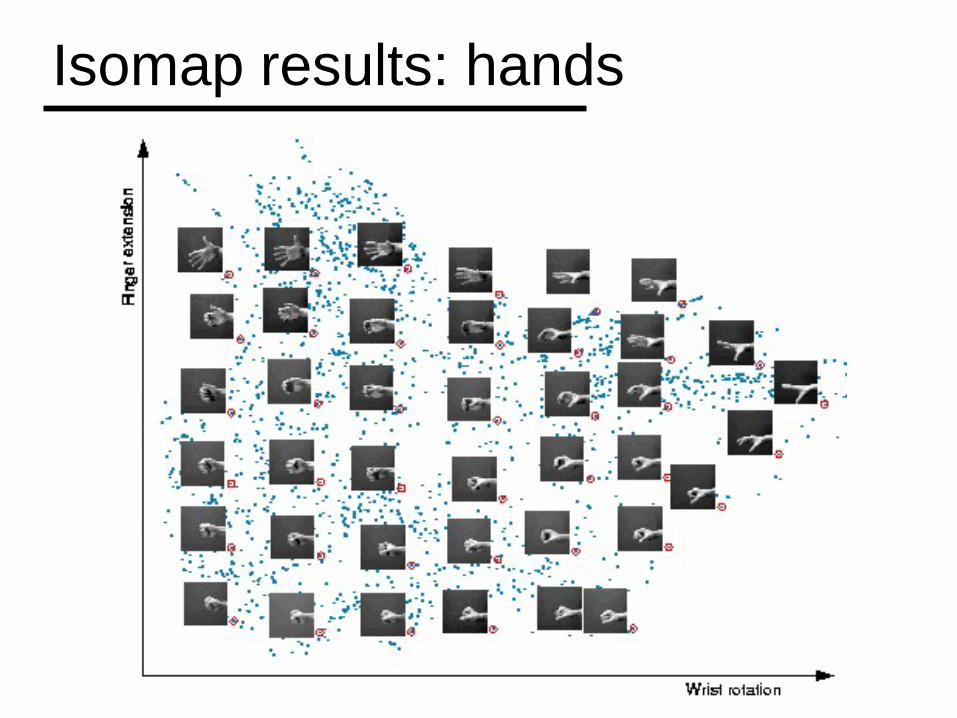
Isomap results: hands
- preserves global structure
- few free parameters
- sensitive to noise, noise edges
- computationally expensive (dense matrix eigen-reduction)
Isomap: pro and con
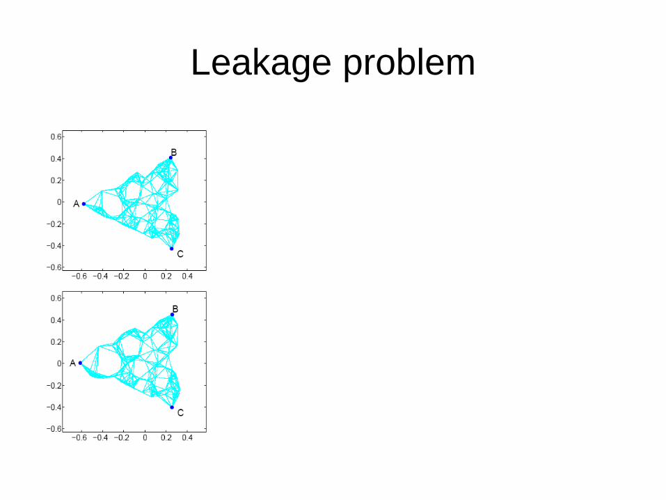
Leakage problem
Find a mapping to preserve local linear relationships between neighbors
Locally Linear Embedding
Locally Linear Embedding
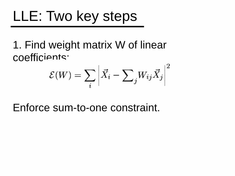
1. Find weight matrix W of linear coefficients:
Enforce sum-to-one constraint.
LLE: Two key steps
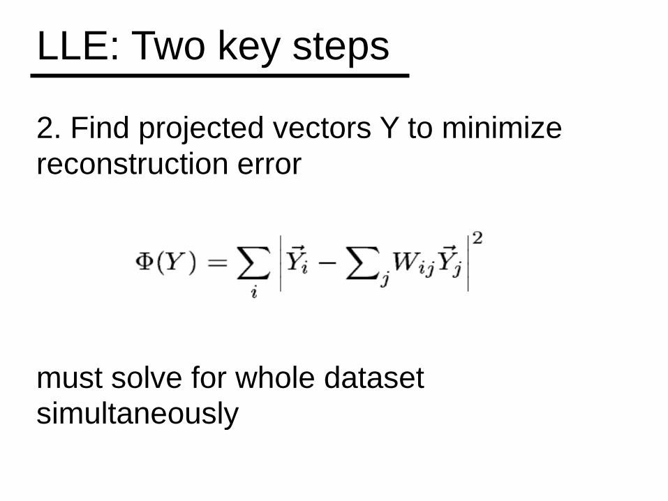
2. Find projected vectors Y to minimize reconstruction error
must solve for whole dataset simultaneously
LLE: Two key steps
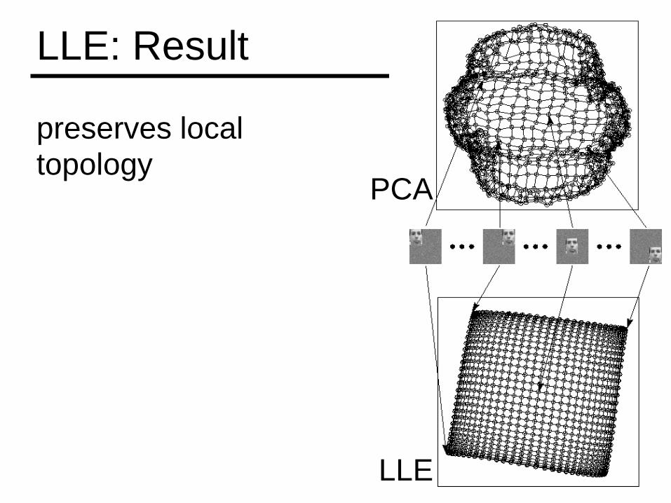
LLE: Result
preserves local topology
PCA
LLE
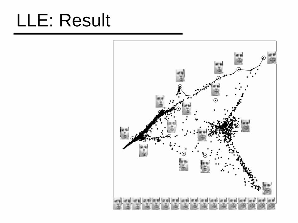
LLE: Result
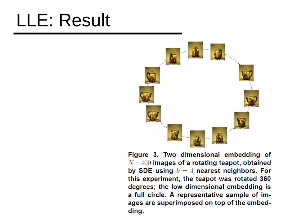
LLE: Result
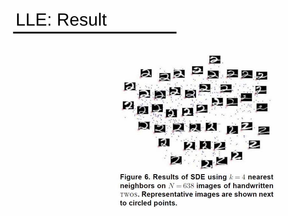
LLE: Result
- no local minima, one free parameter
- incremental & fast
- simple linear algebra operations
- can distort global structure
LLE: pro and con