lecture5 epipolar geometry - Stanford...
20
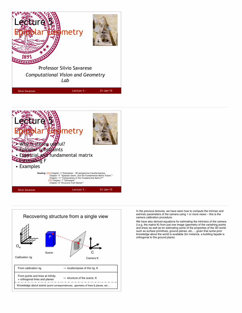
Lecture 5 - Silvio Savarese 21-Jan-15 Professor Silvio Savarese Computational Vision and Geometry Lab Lecture 5 Epipolar Geometry Lecture 5 - Silvio Savarese 21-Jan-15 • Why is stereo useful? • Epipolar constraints • Essential and fundamental matrix • Estimating F • Examples Lecture 5 Epipolar Geometry Reading: [HZ] Chapter: 4 “Estimation – 2D perspective transformations Chapter: 9 “Epipolar Geom. and the Fundamental Matrix Transf.” Chapter: 11 “Computation of the Fundamental Matrix F” [FP] Chapter: 7 “Stereopsis” Chapter: 8 “Structure from Motion” Pinhole perspective projection Recovering structure from a single view C O w P p Calibration rig Scene Camera K From calibration rig From points and lines at infinity + orthogonal lines and planes → structure of the scene, K → location/pose of the rig, K Knowledge about scene (point correspondences, geometry of lines & planes, etc… In the previous lectures, we have seen how to compute the intrinsic and extrinsic parameters of the camera using 1 or more views – this is the camera calibration procedure. We have also derived equations for estimating the intrinsics of the camera (i.e.g, the matrix K) from just one image (geometry of the vanishing points and lines) as well as for estimating some of the properties of the 3D world such as surface primitives, ground planes, etc…, given that some prior knowledge about the world is available (for instance, a building façade is orthogonal to the ground plane).
Transcript of lecture5 epipolar geometry - Stanford...
Lecture 5 - Silvio Savarese 21-Jan-15
Professor Silvio Savarese Computational Vision and Geometry
Lab
Lecture 5 Epipolar Geometry
Lecture 5 - Silvio Savarese 21-Jan-15
• Why is stereo useful? • Epipolar constraints • Essential and fundamental matrix • Estimating F • Examples
Lecture 5 Epipolar Geometry
Reading: [HZ] Chapter: 4 “Estimation – 2D perspective transformations Chapter: 9 “Epipolar Geom. and the Fundamental Matrix Transf.” Chapter: 11 “Computation of the Fundamental Matrix F” [FP] Chapter: 7 “Stereopsis” Chapter: 8 “Structure from Motion”
Pinhole perspective projectionRecovering structure from a single view
COw
Pp
Calibration rigScene
Camera K
From calibration rig
From points and lines at infinity + orthogonal lines and planes → structure of the scene, K
→ location/pose of the rig, K
Knowledge about scene (point correspondences, geometry of lines & planes, etc…
In the previous lectures, we have seen how to compute the intrinsic and extrinsic parameters of the camera using 1 or more views – this is the camera calibration procedure.We have also derived equations for estimating the intrinsics of the camera (i.e.g, the matrix K) from just one image (geometry of the vanishing points and lines) as well as for estimating some of the properties of the 3D world such as surface primitives, ground planes, etc…, given that some prior knowledge about the world is available (for instance, a building façade is orthogonal to the ground plane).

Pinhole perspective projectionRecovering structure from a single view
COw
Pp
Calibration rigScene
Camera K
Why is it so difficult?Intrinsic ambiguity of the mapping from 3D to image (2D)
However, it is in general not possible to recover the structure of the 3D world (e.g., the blue box; the point P) from just one image. This is due to intrinsic ambiguity of the 3D to 2D mapping. Any point along the ray from the camera center C to a point p in the image (line of sight) is a possible candidate for the actual 3D point P.
Recovering structure from a single view
Intrinsic ambiguity of the mapping from 3D to image (2D)
Courtesy slide S. Lazebnik
As we can see in this image, it is easy to fool our eyes about which plane in 3D space, the object that we observe in the image actually belongs to.
Luckily for us, using the ground plane as a cue and the location of the object’s base, our brain can figure out that the tower is actually in the background and that the person is in the foreground.
Two eyes help!What if, however, there are two cameras observing the object? As we will shortly see, it turns out that it is quite helpful! Humans and most other life forms have evolved a pair of eyes so that the world around them can be perceived in 3D. Imagine how it would have been if we were only capable of perceiving 2D images!

O1 O2
pp’
?
Two eyes help!
This is called triangulation
K2 =knownK1 =known
R, T
P= l × "l P
l 'l[Eq. 1]
Here’s how having two eyes (or alternately, cameras) helps. Suppose we have two cameras with known camera intrinsic parameters K
1 and K
2,
respectively, and known relative locations and orientations (i.e., we know the transformations R and T that relate the two camera reference systems). Suppose we have a point P in 3D. Let p and p’ be the observations of P in the images of camera 1 and 2, respectively. The location of P is unknown in the 3D space, but we can measure the locations of p and p’ in each image. Because K
1, K
2, R and T are known,
we can compute the two lines of sight l and l’ which are defined by O1 and
p, and O2 and p’, respectively. Thus, P can be computed as the
intersection point between l and l’ by Eq. 1.This process is known as Triangulation.
• Find P’ that minimizesd(p,M1P')+d(p',M2P')
O1 O2
pp’
P
Triangulation
[Eq. 2]
M1 P’M2 P’
P’
image 1 image 2
In practice, because the observations p and p’ are noisy and the camera calibration parameters may not be accurately estimated, finding the intersection point P using Eq.1 may be problematic (in fact, the exact intersection point may not exist at all). Thus, the triangulation problem is often mathematically characterized by solving the minimization problem expressed in Eq.2. In this equation, we seek to find a point P’ in 3D that best approximates P by minimizing the re-projection error of P’ in both images. What is the re-projection error? The re-projection error for image 1 is computed as the distance between the re-projection of P’ to the image 1 (via projective transformation M
1) and the corresponding observation p;
The re-projection error for image 2 is computed as the distance between the re-projection of P’ to the image 2 (via projective transformation M
2)
and the corresponding observation p’; The overall re-projection error is the sum of these two errors (Eq.2).
Stereo-view geometry
• Correspondence: Given a point p in one image, how can I find the corresponding point p’ in another one?
• Camera geometry: Given corresponding points in two images, find camera matrices, position and pose.
• Scene geometry: Find coordinates of 3D point from its projection into 2 or multiple images.
From stereo-view geometry (i.e., using two images), we can infer information about both the camera geometry as well as the geometry of the scene from observations of points in the image. A key ingredient for doing so is to solve the correspondence problem: given the observations p and p’ in camera 1 and 2 respectively, how do we know that such observations correspond to the same 3D point P, or equivalently, that p and p’ are in correspondence? We will discuss this problem in more details in the next lecture. In this lecture will focus on the geometry that relates camera, points in 3D and corresponding observations– that is, we will focus on what we call the epipolar geometry of a stereo pair.

• Epipolar Plane • Epipoles e, e’
• Epipolar Lines• Baseline
Epipolar geometry
O1 O2
p’
P
p
e e’
= intersections of baseline with image planes = projections of the other camera center
We introduce the following definitions. Let O1 and O
2 be two camera
centers. The line that connects O1 and O
2 is called baseline. O
1 and O
2
and P define the epipolar plane. Let p and p’ be two corresponding points in images 1 and 2. The epipoles e and e’ are defined as the intersections of the baseline and the image planes of camera 1 and 2, respectively. The rays O
1 p and O
2 p’ intersect in the desired 3D coordinate P.
The intersection of the epipolar plane (associated to O1 (or O
2) and the
observations p and p’) with the camera images define the epipolar lines. The line defined by p
and e is an example epipolar line in the image 1;
The line defined by p’ and e’ is an example of epipolar line in the image 2.
The epipolar lines have the property that they all intersect at the corresponding epipoles.
Example of epipolar linesThis slide shows examples of epipolar lines and epipoles associated to the image pair.
O1 O2
P
e’p p’e
Example: Parallel image planes
• Baseline intersects the image plane at infinity• Epipoles are at infinity• Epipolar lines are parallel to x axis
Next we will consider some special cases.
An interesting special case is one in which the image planes are parallel to each other. If the two image planes are parallel to each other, then the epipoles e and e’ will be at infinity, since the line joining the centers O
1O
2
(baseline) is parallel to the image planes.

Example: Parallel Image Planes
e’ at
infinity
e at
infinity
Here is a practical example of two images whose planes are parallel to each other. The epipoles e and e’ occur at infinity. Notice that the epipolar lines in a given image are (almost) parallel to each other and meet at infinity, where the epipoles occur.
Example: Forward translation
• The epipoles have same position in both images• Epipole called FOE (focus of expansion)
O2
e
e’
O1
P
Here is another special case in which there is only a forward translation motion between the two images. In this case, the epipoles will occur at the same location in the two images and are called “focus of expansion”. An example of this configuration is shown to the right.
- Two views of the same object - Suppose I know the camera positions and camera matrices- Given a point on left image, how can I find the corresponding point on right image?
Epipolar Constraint
p
We now pose the following question: Given two images of an object and given a point p on left image (say the tip of the nose), how can I find the corresponding point on right image? Assume that the camera positions, orientations and camera matrices are known.We can use the epipolar geometry to help us answer this question.

Epipolar geometry
O1 O2
P
p p’
Epipolar line 2
Suppose that p is the observation of point P in the 3D world coordinate. The epipolar plane is defined by O
1, p and O
2.
The intersection of the epipolar plane with the camera image planes defines the epipolar lines. Thus, by definition, the corresponding observation p’ in the camera should belong to the epipolar line 2. This puts a constrain on where p’ should be located in the second image. This procedure shows that even without knowing the actual position of P in 3D, by using the concept of epipolar lines (and by assuming that the cameras are calibrated), we can establish a relationship between p and p’ (that is, p’ should belong to the eipolar line 2, which only depends on O
1, p and
O2).
Epipolar Constraint Here is the example
!!!
"
#
$$$
%
&
=→
1vu
PMP
O1 O2
pp’
P
R, T
Epipolar Constraint
!!!
"
#
$$$
%
&'
'
='→
1vu
PMP[Eq. 3] [Eq. 4]
M = K I 0!"
#$
M ' = K ' RT −RTT"#$
%&'
Let us now introduce two important concepts in epipolar geometry: the essential matrix and fundamental matrix— these matrices allow to map points and epipolar lines across views. Let M and M’ be the projection matrices for camera 1 and 2, respectively. M and M’ govern the transformation between 3D world points to 2D image points. Equations 3 and 4 express this transformation for p and p’ (in homogeneous coordinates). Let us assume that the world reference system is associated to camera 1. Let R and T be the rotation matrix and translation vector that transform the “world” coordinates to the camera 2 coordinates. Under this assumption, M’ = K’ [R
T – R
T T ]; we don’t derive this expression here and leave it as
an exercise.

M = K I 0!"
#$
O1 O2
pp’
P
R, T
Epipolar Constraint
K = K’ are known (canonical cameras)
[ ]0IM =
Kcanonical =1 0 00 1 00 0 1
!
"
###
$
%
&&&
M ' = K ' RT −RTT"#$
%&'
M ' = RT −RTT"#$
%&'[Eq. 5] [Eq. 6]
Assume now that the cameras are canonical; that is, K = K’= I. So, the projection matrices can be reduced to the above forms, as given in equations 5 and 6.
T
O1
O2
T = O2 in the camera 1 reference system
R is the rotation matrix such that a vector p’ in the camera 2 is equal to R p’ in camera 1.
The cameras are related by R, T
p’
Camera 1
Camera 2
Specifically, T is the coordinate vector of the translation O1 O
2 separating
the two coordinate systems. T gives the translation between the two cameras and R gives the relative rotation. Using T, we can determine the coordinates of the 2
nd camera center O’. Since the 1
st camera center is
assumed to be at the origin (of the world reference system), then the center (O
2) of the 2
nd camera will be at T.
R is the rotation matrix such that a free vector p’ in the camera 2 is equal to R p’ in camera 1.
O1 O2
pp’
P
R, T
[ ] 0)( =!×⋅→ pRTpT
Epipolar Constraint
is perpendicular to epipolar plane)( pRT !×
pR !=p’ in first camera reference system is
[Eq. 7]
Recall that the inner product between a pair of perpendicular vectors is 0. Since T x (Rp’) is perpendicular to the epipolar plane, we arrive at equation 7.

baba ][0
00
×=
"""
#
$
%%%
&
'
"""
#
$
%%%
&
'
−
−
−
=×
z
y
x
xy
xz
yz
bbb
aaaaaa
Cross product as matrix multiplicationWe can compute the cross product between two given vectors a and b as a matrix-vector multiplication. An example for the case of 3D vectors is illustrated here. In this example, a
x, a
y and a
z (or b
x, b
y and b
z) are the 3
coordinates of a (or b).
O1 O2
pp’
P
R, T
[ ] 0)pR(TpT =!×⋅ [ ] 0pRTpT =!⋅⋅→ ×
E = Essential matrix(Longuet-Higgins, 1981)
Epipolar Constraint
[Eq. 8] [Eq. 9]
We can convert the cross product term into a matrix multiplication and rewrite equation 8 as equation 9. Equation 9 is known as the Epipolar constraint for canonical camera matrices (K=1), and the 3x3 matrix E= [T
x]
R is known as the Essential Matrix. The essential matrix E was first introduced by Longuet-Higgins in 1981.
• l = E p’ is the epipolar line associated with p’ • l’ = ET p is the epipolar line associated with p • E e’ = 0 and ET e = 0 • E is 3x3 matrix; 5 DOF• E is singular (rank two)
Epipolar Constraint
O1 O2
p’
P
p
e e’l l’
pT ⋅ E p' = 0[Eq. 10]
The Essential matrix and two corresponding points p and p’ in the two images satisfy the above Epipolar constraint (given in equation 10). Notice that Eq. 10 is a scalar equation. The Essential matrix is also useful to compute the epipolar lines associated with p and p’. For instance, E p’ is the epipolar line (in the image of camera 1) associated with p’ in the image of camera 2; that is, l = E p’. Similarly, E
T p is the epipolar line
associated with p (l’ = ET
p).E is a 3x3 matrix and has 5 degrees of freedom. Moreover, E is singular and its rank is 2.

Epipolar Constraint
O1 O2
pp’
P
[ ]0IKM =
R, T
M ' = K ' RT −RTT"#$
%&'
pc = K−1 p !pc = K '
−1 !p[Eq. 11] [Eq. 12]
Now, suppose that the cameras are not canonical and let K and K’ be the (unknown) camera matrices for camera 1 and 2, respectively. In this case, we can modify the previous derivation to arrive to a slightly different constraint which we define in the next slide. Let p
c and p’
c be the
projections of P to the corresponding camera images by assuming that the camera matrices are canonical. Let p and p’ be the projections of P to the corresponding camera images by assuming that the cameras are not canonical and defined by K and K’ as above. In this case Eq. 11 and 12 are satisfied.
O1 O2
pp’
P
Epipolar Constraint
pTc ⋅ T×[ ]⋅R #pc = 0 [ ] 0pKRT)pK( 1T1 =!!⋅⋅→ −×
−
[ ] 0pKRTKp 1TT =!!⋅⋅ −×
− 0pFpT =!→ [Eq. 13]
[Eq.9]
pc = K−1 p
!pc = K '−1 !p
Using Eq. 11 and 12, we replace the expressions of pc and p’
c in Eq.9 and,
by follow the above derivation, we obtain a new epipolar constraint, as given in equation 13.
O1 O2
pp’
P
Epipolar Constraint
0pFpT =!
F = Fundamental Matrix(Faugeras and Luong, 1992)
[ ] 1−×
− #⋅⋅= KRTKF TEq. 13
Eq. 14
The epipolar constraint in Eq 13 relates two corresponding points p and p’ in the two images by means of a 3x3 matrix F which we define as the Fundamental Matrix. The fundamental matrix F (characterized by Eq. 14) encapsulates the parameters from both camera matrices (K and K’) as well as the relative translation T and rotation R between them.

Epipolar Constraint
O1 O2
p’
P
p
e e’
• l = F p’ is the epipolar line associated with p’ • l’= FT p is the epipolar line associated with p • F e’ = 0 and FT e = 0• F is 3x3 matrix; 7 DOF • F is singular (rank two)
pT ⋅ F p' = 0
l’l
The fundamental matrix is also useful to compute the epipolar lines associated with p and p‘, when the camera matrices K, K’, and the transformation R and T are unknown. These relationships are equivalent to the ones we introduced for the essential matrix. The key difference is that F has 7 degrees of freedom (instead of 5).
Why F is useful?
- Suppose F is known- No additional information about the scene and camera is given- Given a point on left image, how can I find the corresponding point on right image?
l’ = FT pp
Let us revisit the question we asked earlier:Given two images of an object and given a point p on left image (say the tip of the nose), how can I find the corresponding point on right image? Unlike before, we don’t assume that the camera positions, orientations and camera matrices are known. We assume, however, that F is known. In that case, for a point p in image 1, we can find the epipolar line (F
Tp) in
image 2 associated with p. The corresponding point in image 2 will lie on this epipolar line, as illustrated on the right hand side.
This procedure shows that even without knowing the actual position of P in 3D and without knowing intrinsic and extrinsic parameters of the cameras, by using the concept of epipolar lines, we can establish a relationship between p and p’ (that is, p’ the should belong to the epipolar line F
Tp).
Why F is useful?
• F captures information about the epipolar geometry of 2 views + camera parameters
• MORE IMPORTANTLY: F gives constraints on how the scene changes under view point transformation (without reconstructing the scene!)
• Powerful tool in: • 3D reconstruction • Multi-view object/scene matching
As noted earlier, F encapsulates information about the cameras as well as the geometry of the 2 views. Without the need for explicit reconstruction of the scene, F gives us a way to capture the viewpoint transformation.
Thus, it is also useful in 3D reconstruction and for establishing correspondences between objects from multiple views.

O1 O2
pp’
P
Estimating FThe Eight-Point Algorithm
!!!
"
#
$$$
%
&'
'
='→
1vu
pP!!!
"
#
$$$
%
&
=→
1vu
pP 0pFpT =!
(Hartley, 1995)(Longuet-Higgins, 1981)
Is it possible to estimate F given two images of the same scene and without knowing intrinsic and extrinsic parameters of the cameras? Yes, as long as we have a sufficient number of point correspondences between the two images. There are several algorithms for estimating F. Next, we will discuss the Eight-Point Algorithm which was initially proposed by Longuet-Higgins in 1981 and further extended by R. Hartley in 1995. This algorithms assume that a set of (at least) 8 pairs of corresponding points between two images is available.
0pFpT =!
Estimating F
Let’s take 8 corresponding points
( )11 12 13
21 22 23
31 32 33
', ,1 ' 0
1
F F F uu v F F F v
F F F
! "! "# $# $ =# $# $# $# $% &% &
( )
11
12
13
21
22
23
31
32
33
', ', , ', ', , ', ',1 0
FFFF
uu uv u vu vv v u v FFFFF
! "# $# $# $# $# $# $ =# $# $# $# $# $# $# $% &
[Eq. 13]
[Eq. 14]
We use the fact that the fundamental matrix satisfies the epipolar constraint (Eq. 13) for all the pairs of corresponding points. The constraint in Eq 13 can be rewritten as in Eq. 14. Let’s now consider 8 pairs of corresponding points.
Estimating FThis illustration depicts an example of 8 pairs of corresponding points across these two images. Corresponding points are shown with the same color.

Estimating F
Lsq. solution by SVD!• Rank 8 A non-zero solution exists (unique)
• Homogeneous system
• If N>8 F̂
f
1=f
W 0=f
W
1 1 1 1 1 1 1 1 1 1 1 1
2 2 2 2 2 2 2 2 2 2 2 2
3 3 3 3 3 3 3 3 3 3 3 3
4 4 4 4 4 4 4 4 4 4 4 4
5 5 5 5 5 5 5 5 5 5 5 5
6 6 6 6 6 6 6 6 6 6 6 6
7 7 7 7 7 7
' ' ' ' ' ' 1' ' ' ' ' ' 1' ' ' ' ' ' 1' ' ' ' ' ' 1' ' ' ' ' ' 1' ' ' ' ' ' 1' '
u u u v u v u v v v u vu u u v u v u v v v u vu u u v u v u v v v u vu u u v u v u v v v u vu u u v u v u v v v u vu u u v u v u v v v u vu u u v u v
11
12
13
21
22
23
317 7 7 7 7 7
328 8 8 8 8 8 8 8 8 8 8 8
33
0
' ' ' ' 1' ' ' ' ' ' 1
FFFFFFF
u v v v u vFu u u v u v u v v v u vF
! "! "# $# $# $# $# $# $# $# $# $# $# $ =# $# $# $# $# $# $# $# $# $# $# $# $% &# $
% &
[Eqs. 15]
Each correspondence gives us a constraint (Eq. 14). These constraints can be rearranged to form the homogeneous system in Eqs 15 which can be compactly described as W f = 0. W is a matrix that collects the coordinates u
i, v
i of p
i in image 1 and the coordinates u
i’, v
i’ of p
i’ in image
1, for i=1 to 8. So W is a matrix of measurements. f is a vector that collects all the (unknown) coefficients of the matrix F.The solution to this system of homogeneous equations can be found in the Least Squares sense by Singular Value Decomposition (since Rank(W)=8, which means W is rank deficient). We enforce the constraint that the norm of the solution is unitary (to avoid finding the trivial zero solution). Let F
hat to be the solution of such system.
0pF̂pT =!
and estimated F may have full rank (det(F) ≠0)
0F̂F =−Find F that minimizes
Subject to det(F)=0
But remember: fundamental matrix is Rank2
Frobenius norm (*)
SVD (again!) can be used to solve this problem
^ ^
(*) Sq. root of the sum of squares of all entries
satisfies:F̂Obviously, F
hat satisfies the eipolar constraint in Eq. 13 for every pair of
corresponding points p and p’. However, Fhat
it is not necessarily a proper fundamental matrix. In fact, the fundamental matrix is a rank 2 matrix. But, the way we find the solution (using SVD) does not guarantee that it is a rank 2 matrix. So, we look for a solution that is the best rank-2 approximation of F
hat. In details, we seek an F that minimizes the
Frobenius norm of F-Fhat
subject to the constraint that det(F)=0. The Frobenius norm of a matrix is the square root of the sum of squares of all entries of the matrix. It is possible to show that solution of the above problem can obtained by SVD again;
0F̂F =−Find F that minimizes
Subject to det(F)=0Frobenius norm (*)
F =Us1 0 00 s2 00 0 0
!
"
####
$
%
&&&&
VT
Us1 0 00 s2 00 0 s3
!
"
####
$
%
&&&&
VT = SVD(F̂)
Where:
[HZ] pag 281, chapter 11, “Computation of F”
That is, it can be obtained as U Diag (s1, s2, 0) VT where U diag (s1, s2,
s3) VT = SVD (F
hat), with s1 >= s1 >= s3; See [HZ] pag 281, chapter 11 for
details.

Data courtesy of R. Mohr and B. Boufama.
Here we see an example. Given a set of corresponding pairs of points, we can use the 8-point algorithm to determine F.
Mean errors:10.0pixel9.1pixel
Once we know F, we can also plot the corresponding epipolar lines of each of the points in the two images. We can compute the mean error (distance between epipolar line and the corresponding point) in terms of pixels. Notice a rather significantly large mean error (~10 pixels). To reduce this error, we can consider a modified version of the 8-point algorithm which is called the “Normalized Eight-Point Algorithm” as we will explain next.
Problems with the 8-Point Algorithm
- Recall the structure of W: - do we see any potential (numerical) issue?
F1=f,0=fW Lsq solution
by SVD
What’s the problem with the current version of the Normalized Eight-Point Algorithm? Notice that the constrain under which W f is minimized is not invariant under similarity transformation. Recall the structure of W: do we see any potential (numerical) issue?

1 1 1 1 1 1 1 1 1 1 1 1
2 2 2 2 2 2 2 2 2 2 2 2
3 3 3 3 3 3 3 3 3 3 3 3
4 4 4 4 4 4 4 4 4 4 4 4
5 5 5 5 5 5 5 5 5 5 5 5
6 6 6 6 6 6 6 6 6 6 6 6
7 7 7 7 7 7
' ' ' ' ' ' 1' ' ' ' ' ' 1' ' ' ' ' ' 1' ' ' ' ' ' 1' ' ' ' ' ' 1' ' ' ' ' ' 1' '
u u u v u v u v v v u vu u u v u v u v v v u vu u u v u v u v v v u vu u u v u v u v v v u vu u u v u v u v v v u vu u u v u v u v v v u vu u u v u v
11
12
13
21
22
23
317 7 7 7 7 7
328 8 8 8 8 8 8 8 8 8 8 8
33
0
' ' ' ' 1' ' ' ' ' ' 1
FFFFFFF
u v v v u vFu u u v u v u v v v u vF
! "! "# $# $# $# $# $# $# $# $# $# $# $ =# $# $# $# $# $# $# $# $# $# $# $# $% &# $
% &
Problems with the 8-Point Algorithm
• Highly un-balanced (not well conditioned)• Values of W must have similar magnitude• This creates problems during the SVD decomposition
0=Wf
HZ
pag
108
Yes! W is not a well conditioned matrix (un-balanced) due to the fact that the values of W are not necessarily in the same order of magnitude.This creates problems during the SVD decomposition. See HZ pag 108 for details.
Normalization
IDEA: Transform image coordinates such that the matrix W becomes better conditioned (pre-conditioning)
For each image, apply a following transformation T (translation and scaling) acting on image coordinates such that:
• Origin = centroid of image points• Mean square distance of the image points from origin is ~2 pixels
ii pTq = ii pTq !!=! (normalization)
A way to fix this is to normalize the points in the image before solving for W f = 0. That is, transform the image coordinates such that the matrix W becomes better conditioned (pre-conditioning).
Image points are normalized by applying a transformation T (translation and scaling) acting on image coordinates such that:1. The origin of the new coordinate system is located at the centroid of
the image points (in the old coordinate system)2. The mean square distance of the transformed image points from origin
is ~2 pixels
Notice that we apply a transformation T on image 1 and a (possible) different transformation T’ on image 2.Let us call q
i and q
i’ the normalized points p
i and p’
I in image 1 and 2,
respectively.
After that, we apply the same procedure as before on qi and q
i’ for i=1 to
8.
Coordinate system of the image before applying T
Coordinate system of the image after applying T
T
2 pixels
Example of normalization
• Origin = centroid of image points• Mean square distance of the image points from origin is ~2 pixels
Here is an example of the effect of T on the image points (for one of the image pair).

1. Normalize coordinates in images 1 and 2:
2. Use the eight-point algorithm to compute from the corresponding points q and q’ .
1. Enforce the rank-2 constraint.
2. De-normalize Fq:
i i
ii pTq = ii pTq !!=!
0qFq qT =!
The Normalized Eight-Point Algorithm
qF→
'TFTF qT= 0)Fdet( q =
0. Compute T and T’ for image 1 and 2, respectively
F̂q
such that:
Thus, the modified version of the Eight-Point Algorithm is summarized above. Once F
q
hat is computed and the rank-2 constraint is enforced, the
matrix Fq is de-normalized by inverting the transformation , and F is
obtained as: F = TT F
q T’.
With
tran
sfor
mat
ion
With
out t
rans
form
atio
n Mean errors:10.0pixel9.1pixel
Mean errors:1.0pixel0.9pixel
Notice the mean error has been significantly reduced.
Lecture 5 - Silvio Savarese 21-Jan-15
• Why is stereo useful? • Epipolar constraints • Essential and fundamental matrix • Estimating F • Examples
Lecture 5 Epipolar Geometry
Reading: [AZ] Chapter: 4 “Estimation – 2D perspective transformations Chapter: 9 “Epipolar Geometry and the Fundamental Matrix Transformation” Chapter: 11 “Computation of the Fundamental Matrix F” [FP] Chapter: 7 “Stereopsis” Chapter: 8 “Structure from Motion”
In the next slides we will show an example E and F for the special case that images are parallel.

O1 O2
P
e’p p’
e
Example: Parallel image planes
E=?
K K
K1=K2 = knownHint :
x
y
z
x parallel to O1O2
R = I T = (T, 0, 0)
Let us try to compute the essential matrix E in the case of parallel image planes. We assume that the two cameras have the same K, and that K is known. Since the image planes are parallel, there is no relative rotation between the two cameras. So, R = I. There is only a translation T, along the x-axis. So, T = (T,0,0). With this information, we set out to find E…
!!!
"
#
$$$
%
&
−=!!!
"
#
$$$
%
&
−
−
−
=
0000
000
00
0
TT
TTTTTT
xy
xz
yz
IE
Essential matrix for parallel images
T = [ T 0 0 ]R = I
[ ] RTE ⋅= ×
[Eq. 20]
Recall that E can be computed as the cross product of T and R. Using matrix multiplication to compute the cross product (as described in the previous slides), it is easy to reduce E to the form in equation 20.
O1
P
e’p p’e
Example: Parallel image planes
K K
x
y
z
horizontal!What are the directions of epipolar lines?
l = E p' =0 0 00 0 −T0 T 0
"
#
$$$
%
&
'''
uv1
"
#
$$$
%
&
'''=
0−TTv
"
#
$$$
%
&
'''
l l’
Once E is known, we can find the directions of the epipolar lines associated with points in the image planes. Let us compute the direction of the epipolar line l associated with point p’, as E p’. We can see that the direction of l is horizontal, as we would expect to see in this case. We can perform E p to compute l’, which can also be verified to be horizontal.

Example: Parallel image planes
How are p and p’ related?
pT ⋅ E p' = 0
P
e’p p’
e
K Ky
z
xO1
As we have seen before, we can relate p and p’ through the Epipolar constraint.
Example: Parallel image planes
( ) ( )T
0 0 0 0p E p 0 1 0 0 0 1 0
0 0 1
uu v T v u v T Tv Tv
T Tv
!" # $ % $ %& ' & '( )! ! != ⇒ − = ⇒ − = ⇒ =& ' & '( )& ' & '!( ), - . / . /
How are p and p’ related?
P
e’p p’
e
K Ky
z
O1x
⇒ v = "v
We can use the Epipolar constraint to relate the y coordinates of p and p’. As the slide shows, v = v’ which implies that p and p’ share the same v-coordinate as expected.
Example: Parallel image planes
Rectification: making two images “parallel” Why it is useful? • Epipolar constraint → v = v’
• New views can be synthesized by linear interpolation
P
e’p p’
e
K Ky
z
O1x
Rectification is the process of making two given images parallel. It is useful because there is a straightforward relationship between corresponding points (they share the same v coordinate) when two images are rectified; also, it possible to synthesize novel intermediate views by simple linear interpolation of the two parallel images. This technique is called view morphing as explained next.

Application: view morphingS. M. Seitz and C. R. Dyer, Proc. SIGGRAPH 96, 1996, 21-30
This technique was first introduced by Seitz and Dyer in 1996. We see an example here.
Rectification
u
u
u
v
v
v
î2
î1
îS
I1
I2
Is
P
C2
Cs
C1
H1
H2
In view morphing, we first convert the two images into the parallel configuration. This step is known as pre-warping, and is done using two homographies H
1 and H
2 for images I
1 and I
2. We then linearly interpolate
positions and intensities of corresponding pixels in I1 and I
2 to form I
s.
Finally, we post-warp Is using a homography H
s to obtain the final desired
image.
Here is we see some example of view morphing.

Morphing without rectifyingNotice that the pre-warping (rectification) step is critical. This is an example where two images are morphed without pre-warping. Clearly, severe distortions are generated during the morphing.

From its reflection!
http://danielwedge.com/fmatrix/
The Fundamental Matrix Song