CSC2515  Winter  2015    Introduc3on  to  Machine  Learning  

   

Lecture  4:  Neural  Networks  

 All  lecture  slides  will  be  available  as  .pdf  on  the  course  website:  http://www.cs.toronto.edu/~urtasun/courses/CSC2515/

CSC2515_Winter15.html  

1

Limita3ons  of  linear  classifiers  •  Linear  classiCiers  (e.g.,  logistic  regression)  classify  inputs  based  on  linear  combinations  of  features  xi  

•  Many  decisions  involve  non-­‐linear  functions  of  the  input  

•  Canonical  example:  do  2  input  elements  have  the  same  value?  Same:          (1,1)  à  1;    (0,0)  à  1      Diff:            (1,0)  à  0;    (0,1)  à  0  

Data Space

0,1

0,0 1,0

1,1

output =1 output =0

The positive and negative cases cannot be separated by a plane 2

How  to  construct  nonlinear  classifiers?  

•  Would  like  to  construct  non-­‐linear  discriminative  classiCiers  that  utilize  functions  of  input  variables  

•  Two  approaches:  –  Add  inCinite  number  of  extra  functions    

•  Need  to  address  over-­‐Citting  –  Add  Cinite  but  large  number  of  extra  functions  

•  If  these  functions  are  Cixed  (Gaussian,  sigmoid,  polynomial  basis  functions),    then  the  optimization  still  involves  linear  combinations  of  (Cixed  functions  of)  the  inputs  

•  Or  we  can  make  these  functions  depend  on  additional  parameters  à  need  an  efCicient  method  of  training  extra  parameters  

  3

Neural  networks  

•  Many  machine  learning  methods  inspired  by  biology,  brains  

•  Our  brains  contain  ~1011  neurons,  each  of  which  communicates  to  ~104  other  neurons  

•  Multi-­‐layer  perceptron,  or  neural  network,  is  a  popular  supervised  learning  approach  

•  DeCines  extra  functions  of  the  inputs  (hidden  features),  computed  by  neurons  

•  ArtiCicial  neurons  called  units  •  Network  output  is  linear  combination  of  hidden  units  

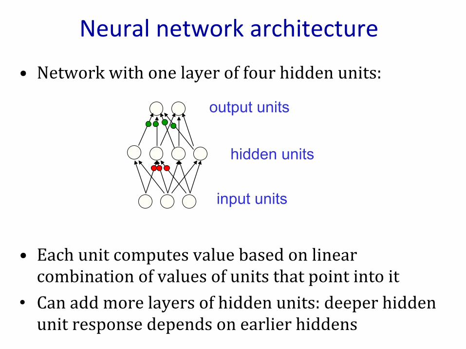
•  Network  with  one  layer  of  four  hidden  units:  

•  Each  unit  computes  value  based  on  linear  combination  of  values  of  units  that  point  into  it  

•  Can  add  more  layers  of  hidden  units:  deeper  hidden  unit  response  depends  on  earlier  hiddens  

Neural  network  architecture  

output units

input units

hidden units

•  Output  of  network  can  be  written  as  follows,  with  k  indexing  the  two  output  units:  

   

•  Network  with  non-­‐linear  activation  function  f()  is  a  universal  approximator  (esp.  with  increasing  J)  

•  Standard  choice  of  activation  function:  sigmoid/logistic,  or  tanh,  or  rectiCied  linear  (relu)        tanh(z)  =  (exp(z)  –  exp(-­‐z))/(exp(z)  +  exp(-­‐z))  

             relu(z)  =  max(0,z)  

What  does  the  network  compute?  

output units

input units

ok (x) = g(wk0 + hj (x)wkj )j=1

J

∑

hj (x) = f (wj0 + xivji )i=1

D

∑

hidden units

Example  applica3on  •  Consider  trying  to  classify  image  of  handwritten  digit:  32x32  pixels  

•  Single  output  units  –  it  is  a  4  (one  vs.  all)?  •  Use  the  sigmoid  output  function:  

•  Can  train  the  network,  that  is,  adjust  all  the  parameters  w,  to  optimize  the  training  objective,  but  this  is  a  complicated  function  of  the  parameters    

ok =1

1+ exp(−zk )

zk = (wk0 + hj (x)vkj )j=1

J

∑

Back-­‐propagation:  an  efCicient  method  for  computing  gradients  needed  to  perform  gradient-­‐based  optimization  of  the  weights  in  a  multi-­‐layer  network  

   Loop  until  convergence:  •  For  each  example  n  

1)  Input  x(n) ,  propagate  activity  forward  (x(n)    à  h(n)  à  o(n))  2)  Propagate  gradients  backward    3)  Update  each  weight  (via  gradient  descent)  

Given  any  error  function  E,  activation  functions  g()  and  f(),  just  need  to  derive  gradients  

Training  mul3-­‐layer  networks:  back-­‐propaga3on  

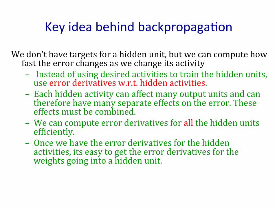
Key  idea  behind  backpropaga3on  

We  don’t  have  targets  for  a  hidden  unit,  but  we  can  compute  how  fast  the  error  changes  as  we  change  its  activity  –   Instead  of  using  desired  activities  to  train  the  hidden  units,  use  error  derivatives  w.r.t.  hidden  activities.  

–  Each  hidden  activity  can  affect  many  output  units  and  can  therefore  have  many  separate  effects  on  the  error.  These  effects  must  be  combined.  

–  We  can  compute  error  derivatives  for  all  the  hidden  units  efCiciently.    

–  Once  we  have  the  error  derivatives  for  the  hidden  activities,  its  easy  to  get  the  error  derivatives  for  the  weights  going  into  a  hidden  unit.  

Non-­‐linear  neurons  with  smooth  deriva3ves  

•  For  backpropagation,  we  need  neurons  (units)  that  have  well-­‐behaved  derivatives.  –  Typically  they  use  the  logistic  function  

–  The  output  is  a  smooth  function  of  the  inputs  and  the  weights.  

x j = bj + yii∑ wij

yj =1

1+ e−x j

∂x j∂wij

= yi∂x j∂yi

= wij

dyjdx j

= yj (1− yj )0.5

0 0

1

jx

jy

Its odd to express it in terms of y. 10

Back-­‐propaga3on:  sketch  on  one  training  case  1.  Convert  discrepancy  between  

each  output  and  its  target  value  into  an  error  derivative.  

2.  Compute  error  derivatives  in  each  hidden  layer  from  error  derivatives  in  layer  above.  [assign  blame  for  error  at  k  to  each  unit  j  according  to  its  inCluence  on  k  (depends  on  wkj)]  

3.  Use  error  derivatives  w.r.t.  activities  to  get  error  derivatives  w.r.t.  the  weights.  

j

k

kkk

kk

k

hE

oE

tooE

toE

∂

∂

∂

∂

−=∂

∂

−= ∑ 221 )(

The  deriva3ves  

∑∑ ∂

∂=

∂

∂=

∂

∂

∂

∂=

∂

∂

∂

∂=

∂

∂

∂

∂−=

∂

∂=

∂

∂

j jij

j ji

j

i

ji

jij

j

ij

jjj

jj

j

j

xEw

xE

dydx

yE

xEy

xE

wx

wE

yEyy

yE

dxdy

xE )1(j

i i

j

j

y

x

y

12

Ways  to  use  weight  deriva3ves  

•  How  often  to  update  –  after  each  training  case?  –  after  a  full  sweep  through  the  training  data?  –  after  a  “mini-­‐batch”  of  training  cases?  

•  How  much  to  update  – Use  a  Cixed  learning  rate?  – Adapt  the  learning  rate?  – Add  momentum?

13

)()()()(

1

)( )1()( ni

nk

nk

nk

N

n

nkki

kikiki xootow

wEww −−−=

∂

∂−← ∑

=

ηη

wki ← wki −η∂E∂wki

+βΔwki (t −1)

When  using  a  neural  network  as  a  function  approximator  (regressor)    sigmoid  activation  and  MSE  work  well  

 For  classiCication,  if  it  is  a  binary  (2-­‐class)  problem,  then  cross-­‐entropy  error  function  often  does  better  (as  we  saw  with  logistic  regression)  

             

Choosing  ac3va3on  and  cost  func3ons  

o(n) = 11+exp(−z(n) )

E = − t (n) logo(n) + (1− t (n) ) log(1−o(n) )n∑

∂E∂o

= o− t

∂o∂z

= o(1−o)

∂E∂z

=∂E∂o

∂o∂z

= (o− t)o(1−o)

Some  Success  Stories  

•  Back-­‐propagation  has  been  used  for  a  large  number  of  practical  applications.  – Recognizing  hand-­‐written  characters  – Recognize  speech  – Predicting  the  next  word  in  a  sentence  from  the  previous  words  

– Autonomous  vehicle  control  – Recognizing  objects  in  images  

 

A  basic  problem  in  speech  recogni3on  

•  We  cannot  identify  phonemes  perfectly  in  noisy  speech  –  The  acoustic  input  is  often  ambiguous:  there  are  several  different  words  that  Cit  the  acoustic  signal  equally  well.  

•  People  use  their  understanding  of  the  meaning  of  the  utterance  to  hear  the  right  word.  –  We  do  this  unconsciously  –  We  are  very  good  at  it  

•  This  means  speech  recognizers  have  to  know  which  words  are  likely  to  come  next  and  which  are  not.  –  Can  this  be  done  without  full  understanding?  

16

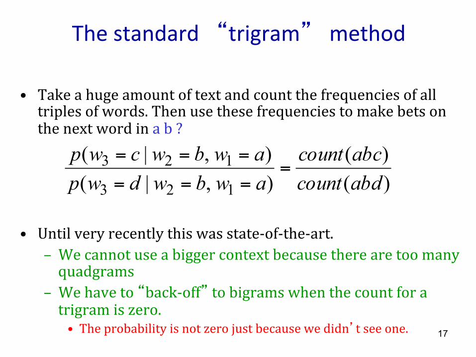
•  Take  a  huge  amount  of  text  and  count  the  frequencies  of  all  triples  of  words.  Then  use  these  frequencies  to  make  bets  on  the  next  word  in  a  b  ?  

•  Until  very  recently  this  was  state-­‐of-­‐the-­‐art.  –  We  cannot  use  a  bigger  context  because  there  are  too  many  quadgrams  

–  We  have  to  “back-­‐off”  to  bigrams  when  the  count  for  a  trigram  is  zero.  •  The  probability  is  not  zero  just  because  we  didn’t  see  one.    

 

The  standard  “trigram”  method  

)()(

),|(),|(

123

123abdcountabccount

awbwdwpawbwcwp

====

===

17

Why  the  trigram  model  is  limited   •  Suppose  we  have  seen  the  sentence  “the  cat  got  squashed  in  the  garden  on  friday”  

•  This  should  help  us  predict  words  in  the  sentence  “the  dog  got  Clattened  in  the  yard  on  monday”  

•  A  trigram  model  does  not  understand  the  similarities  between  –  cat/dog      squashed/Clattened      garden/yard      friday/monday  

•  To  overcome  this  limitation,  we  need  to  use  the  features  of  previous  words  to  predict  features  of  the  next  word  –  Using  a  feature  representation  and  a  learned  model  of  how  past  features  predict  future  ones,  we  can  use  many  more  words  from  the  past  history.  

   18

Softmax

iij i

j

ji

jj

j

iii

i

j

x

x

i

dyxy

yC

xC

ydC

yyxy

e

eyj

i

−=∂

∂

∂

∂=

∂

∂

−=

−=∂

∂

=

∑

∑

∑

log

)(1

Handling multiple classes: the output units use a non-local non-linearity:

The cost function is the negative log prob of the right answer

output units

x

y

x

y

x

y 1

1 2

2 3

3

desired value

19

A  neural  net  for  predic3ng  the  next  word  

Softmax units (one per possible word)

Index of word at t-2 Index of word at t-1

Learned distributed encoding of word t-2

Learned distributed encoding of word t-1

Units that learn to predict the output word from features of the input words

output

inputs

Table look-up Table look-up

Skip-layer connections

20

An  alterna3ve  architecture  

Index of word at t-2

Learned distributed encoding of word t-2

Units that discover good or bad combinations of features

Index of word at t-1

Learned distributed encoding of word t-1

Index of candidate

Learned distributed encoding of candidate

Try all candidate words one at a time

A single output unit that gives a score for the candidate word in this context

Use the scores from all candidate words in a softmax to get error derivatives that try to raise the score of the correct candidate and lower the score of its high-scoring rivals.

21

Applying  backpropaga3on  to  shape  recogni3on  

•  People  are  very  good  at  recognizing  shapes  –  Intrinsically  difCicult,  computers  are  bad  at  it  

•  Some  reasons  why  it  is  difCicult:  –  Segmentation:  Real  scenes  are  cluttered  –  Invariances:  We  are  very  good  at  ignoring  all  sorts  of  variations  that  do  not  affect  shape  

– Deformations:  Natural  shape  classes  allow  variations  (faces,  letters,  chairs)  

– A  huge  amount  of  computation  is  required  22

The  invariance  problem  

•  Our  perceptual  systems  are  very  good  at  dealing  with  invariances  –  translation,  rotation,  scaling  – deformation,  contrast,  lighting,  rate  

•  We  are  so  good  at  this  that  its  hard  to  appreciate  how  difCicult  it  is  –  Its  one  of  the  main  difCiculties  in  making  computers  perceive  

– We  still  don’t  have  generally  accepted  solutions  

23

The  replicated  feature  approach  •  Adopt  approach  apparently  used  in  monkey  

visual  systems  •  Use  many  different  copies  of  the  same  

feature  detector.    –  Copies  have  slightly  different  positions.  –  Could  also  replicate  across  scale  and  orientation.    •  Tricky  and  expensive  

–  Replication  reduces  number  of  free  parameters  to  be  learned.  

•  Use  several  different  feature  types,  each  with  its  own  replicated  pool  of  detectors.  –  Allows  each  patch  of  image  to  be  represented  in  several  ways.  

 

The red connections all have the same weight.

24

Backpropaga3on  with  weight  constraints  

•  It  is  easy  to  modify  the  backpropagation  algorithm  to  incorporate  linear  constraints  between  the  weights.  

•  We  compute  the  gradients  as  usual,  and  then  modify  the  gradients  so  that  they  satisfy  the  constraints.  –  So  if  the  weights  started  off  satisfying  the  constraints,  they  will  continue  to  satisfy  them.  

2121

21

21

21

:

::

wandwforwE

wEuse

wEand

wEcompute

wwneedwewwconstrainTo

∂

∂+

∂

∂

∂

∂

∂

∂

Δ=Δ

=

25

Le  Net  

•  Yann  LeCun  and  others  developed  a  really  good  recognizer  for  handwritten  digits  by  using  backpropagation  in  a  feedforward  net  with:  – Many  hidden  layers  – Many  pools  of  replicated  units  in  each  layer.  – Averaging  the  outputs  of  nearby  replicated  units.  

– A  wide  net  that  can  cope  with  several  characters  at  once  even  if  they  overlap.  

•  Demos  of  LENET  at  http://yann.lecun.com  26

Recognizing  Digits  Hand-­‐written  digit  recognition  network  

–  7291  training  examples,  2007  test  examples  –  Both  contain  ambiguous  and  misclassiCied  examples  –  Input  pre-­‐processed  (segmented,    normalized)  

•  16x16  gray  level  [-­‐1,1],  10  outputs  

27

LeNet:  Summary  Main  ideas:  

•  Local  à  global  processing  •  Retain  coarse  posn  info  

Main  technique:  weight  sharing  –  units  arranged  in  feature  maps  

 Connections:  1256  units,  64,660  

cxns,  9760  free  parameters    Results:    0.14%  (train),  5.0%  

(test)    vs.  3-­‐layer  net  w/  40  hidden  units:    1.6%  (train),  8.1%  (test)  

28

The  82  errors  made  by  LeNet5  

Notice that most of the errors are cases that people find quite easy.

The human error rate is probably 20 to 30 errors

29

A  brute  force  approach  

•  LeNet  uses  knowledge  about  the  invariances  to  design:  –   the  network  architecture    –  or  the  weight  constraints    –  or  the  types  of  feature  

•  But  its  much  simpler  to  incorporate  knowledge  of  invariances  by  just  creating  extra  training  data:  –  for  each  training  image,  produce  new  training  data  by  applying  all  of  the  transformations  we  want  to  be  insensitive  to  

–  Then  train  a  large,  dumb  net  on  a  fast  computer.  –  This  works  surprisingly  well  

30

Fabrica3ng  training  data  

Good  generalization  requires  lots  of  training  data,  including  examples  from  all  relevant  input  regions  

Improve  solution  if  good  data  can  be  constructed    Example:  ALVINN  

31

ALVINN:  simula3ng  training  examples  

On-­‐the-­‐Cly  training:  current  video  camera  image  as  input,  current  steering  direction  as  target  

But:  over-­‐train  on  same  inputs;  no  experience  going  off-­‐road  

Method:  generate  new  examples  by  shifting  images    

Replace  10  low-­‐error  &  5  random  training  examples  with  15  new  

Key:  relation  between  input  and  output  known!  

32

Making  backpropaga3on  work  for  recognizing  digits  

•  Using  the  standard  viewing  transformations,  and  local  deformation  Cields  to  get  lots  of  data.  

•  Use  many,  globally  connected  hidden  layers  and  learn  for  a  very  long  time  – This  requires  a  GPU  board  or  a  large  cluster      

•  Use  the  appropriate  error  measure  for  multi-­‐class  categorization  – Cross-­‐entropy,  with  softmax  activation  

•  This  approach  can  get  35  errors  on  MNIST!   33

34

OverfiWng •  The  training  data  contains  information  about  the  regularities  in  the  mapping  from  input  to  output.  But  it  also  contains  noise  –  The  target  values  may  be  unreliable.  –  There  is  sampling  error.  There  will  be  accidental  regularities  just  because  of  the  particular  training  cases  that  were  chosen  

•  When  we  Cit  the  model,  it  cannot  tell  which  regularities  are  real  and  which  are  caused  by  sampling  error.    –  So  it  Cits  both  kinds  of  regularity.  –  If  the  model  is  very  Clexible  it  can  model  the  sampling  error  really  well.  This  is  a  disaster.  

35

Preven3ng  overfiWng  

•  Use  a  model  that  has  the  right  capacity:  –  enough  to  model  the  true  regularities  – not  enough  to  also  model  the  spurious  regularities  (assuming  they  are  weaker)  

•  Standard  ways  to  limit  the  capacity  of  a  neural  net:  –  Limit  the  number  of  hidden  units.  –  Limit  the  size  of  the  weights.  –  Stop  the  learning  before  it  has  time  to  overCit.  

36

Limi3ng  the  size  of  the  weights  

Weight-­‐decay  involves  adding  an  extra  term  to  the  cost  function  that  penalizes  the  squared  weights.  

–  Keeps  weights  small  unless  they  have  big  error  derivatives.  

ii

i

iii

ii

wEw

wCwhen

wwE

wC

wEC

∂

∂−==

∂

∂

+∂

∂=

∂

∂

∑+=

λ

λ

λ

1

22

,0

w

C

37

The  effect  of  weight-­‐decay  

•  It  prevents  the  network  from  using  weights  that  it  does  not  need  –  This  can  often  improve  generalization  a  lot.    –  It  helps  to  stop  it  from  Citting  the  sampling  error.    –  It  makes  a  smoother  model  in  which  the  output  changes  more  slowly  as  the  input  changes.  

•  But,  if  the  network  has  two  very  similar  inputs  it  prefers  to  put  half  the  weight  on  each  rather  than  all  the  weight  on  one  à  other  form  of  weight  decay?  

w/2 w/2 w 0

38

Deciding  how  much  to  restrict  the  capacity  

•  How  do  we  decide  which  limit  to  use  and  how  strong  to  make  the  limit?  –  If  we  use  the  test  data  we  get  an  unfair  prediction  of  the  error  rate  we  would  get  on  new  test  data.  

–  Suppose  we  compared  a  set  of  models  that  gave  random  results,  the  best  one  on  a  particular  dataset  would  do  better  than  chance.    But  it  won’t  do  better  than  chance  on  another  test  set.    

•  So  use  a  separate  validation  set  to  do  model  selection.  

39

Using  a  valida3on  set  

•  Divide  the  total  dataset  into  three  subsets:  – Training  data  is  used  for  learning  the  parameters  of  the  model.  

– Validation  data  is  not  used  for  learning  but  is  used  for  deciding  what  type  of  model  and  what  amount  of  regularization  works  best  

– Test  data  is  used  to  get  a  Cinal,  unbiased  estimate  of  how  well  the  network  works.  We  expect  this  estimate  to  be  worse  than  on  the  validation  data  

•  We  could  then  re-­‐divide  the  total  dataset  to  get  another  unbiased  estimate  of  the  true  error  rate.  

40

Preven3ng  overfiWng  by  early  stopping  

•  If  we  have  lots  of  data  and  a  big  model,  its  very  expensive  to  keep  re-­‐training  it  with  different  amounts  of  weight  decay  

•  It  is  much  cheaper  to  start  with  very  small  weights  and  let  them  grow  until  the  performance  on  the  validation  set  starts  getting  worse  

•  The  capacity  of  the  model  is  limited  because  the  weights  have  not  had  time  to  grow  big.  

41

Why  early  stopping  works  

•  When  the  weights  are  very  small,  every  hidden  unit  is  in  its  linear  range.  –  So  a  net  with  a  large  layer  of  hidden  units  is  linear.  

–  It  has  no  more  capacity  than  a  linear  net  in  which  the  inputs  are  directly  connected  to  the  outputs!  

•  As  the  weights  grow,  the  hidden  units  start  using  their  non-­‐linear  ranges  so  the  capacity  grows.  

outputs

inputs

42