LLNL-PRES-668311 This work was performed under the auspices of the U.S. Department of Energy by Lawrence Livermore National Laboratory under Contract DE-AC52-07NA27344. Lawrence Livermore National Security, LLC

Lecture Notes on

Radiation Transport for Spectroscopy

ICTP-IAEA School on Modern Methods in Plasma Spectroscopy

March 16-20, 2015 Trieste, Italy

Outline •  Definitions, assumptions and terminology

•  Equilibrium limit

•  Radiation transport equation •  Characteristic form & formal solution

•  Material radiative properties

•  Absorption, emission, scattering •  Coupled systems

•  LTE / non-LTE •  Line radiation

•  Line shapes

•  Redistribution •  Material motion

•  Solution methods •  Transport operators

•  2-level & multi-level atoms

•  Escape factors

Radiation Transport for Spectroscopy

Basic assumptions

Classical / Semi-classical description –

•  Radiation field described by either specific intensity Iν or the photon

distribution function fν

•  Unpolarized radiation

•  Neglect index of refraction effects (n≈1, ω>>ωp)

! Photons travel in straight lines

•  Neglect true scattering (mostly)

•  Static material (for now)

! Single reference frame

Macroscopic - specific intensity Iν

•  energy per (area x solid angle x time) within

the frequency range

•  dE = energy crossing area dA within

Microscopic - photon distribution function

Radiation Description

thin

dE = I

v

!r ,Ω,t( )

!n •!Ω( )dAdΩdv dt

dE = hv( )spins

∑ fν

!r ,!p,t( )

d 3!xd 3 !p

h3

I

v= 2

hv3

c2fν

!r ,!p,t( )

(ν ,ν + dν )

(dΩdv dt)

!p =

hv

c

!Ω

0th moment = energy density x c/4π

1st moment = flux x 1 /4π

2nd moment = pressure tensor x c /4π

For isotropic radiation, Kν is diagonal with equal elements:

In this case, radiation looks like an ideal gas with = 4/3

Jν=

1

4πIν

dΩ∫

Hν=

1

4πnI

νdΩ∫

Kν=

1

4πnnI

νdΩ∫

K

ν=

1

3Jν

I (P =1

3E)

Angular Moments

γ

Thermal Equilibrium

Intensity: Planck function Distribution function: Bose-Einstein

Energy density

For Te=Tr and nH = 1023 cm-3 :

Bv= 2

hv3

c2

1

ehv

kTr −1

fν=

1

ehv

kTr −1

Erad

Tr

( ) =4π

cB

vT

r( )

0

∞

∫ dv = aTr

4

Erad

= Ematter

⇔ T ≈ 300eV

!"#!"#$%&'!()*+,$-./&,0%!1230'04+03,5!6!

!7&+8%'*9!)&:*!;)*+,&'!-09;+0438$/9!"(*<!(05!

!7)$;$/!-09;+0438$/!%&/!4*!&+40;+&+.!

•  Boltzmann equation for the photon distribution function:

•  The LHS describes the flow of radiation in phase space

•  The RHS describes absorption and emission

•  Absorption & emission coefficients depend on atomic physics

•  Photon # is not conserved (except for scattering)

•  Photon mean free path

Radiation Transport Equation

= absorption coefficient (fraction of energy absorbed per unit length)

= emissivity (energy emitted per unit time, volume, frequency, solid angle)

1

c

∂ Iv

∂ t+

!Ω i∇I

v= −α

vI

v+η

v

1

c

∂ fν

∂ t+

!Ω i∇fν =

∂ fν

∂ t

coll

α

v

η

v

Iv= 2hν

hνc

2

fν

λν= 1/α

ν

Characteristic Form

Define the source function Sν and optical depth τ

ν:

Sν = η

ν/αν = B

ν in LTE dτ

ν = α

ν ds

Along a characteristic, the radiation transport equation becomes

This solution is useful when material properties are fixed, e.g.

postprocessing for diagnostics

Important features:

•  Explicit non-local relationship between Iν and S

ν

•  Escaping radiation comes from depth τν ≈ 1

•  Implicit Sν(Iν) dependence comes from radiation / material coupling

!

dIv

dτv

= − Iv+ S

v⇒ I

vτ

v( ) = I

v0( )e−τ

v + e− τ

v− ′τν( )

Sv

′τν( )

0

τv

∫ d ′τν

Self-consistently determining Sν and I

ν is

the hard part of radiation transport

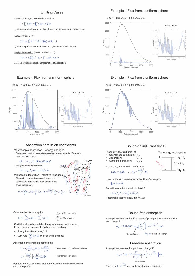
Limiting Cases

Optically-thin τν<<1 (viewed in emission):

Iν reflects spectral characteristics of emission, independent of absorption

Optically-thick τν>>1:

Iν reflects spectral characteristics of S

ν (over ~last optical depth)!

Negligible emission (viewed in absorption):

Iν / Iν(0) reflects spectral characteristics of absorption

I

v= S

v0

τv

∫ d ′τν = ηv

0

dx

∫ d ′x →ηvdx

I

vτ

v( ) = e

− τv− ′τν( )

Sv

′τν( )

0

τv

∫ d ′τν→ S

vτν( )

I

vτ

v( ) = I

v0( )e−τ

v , τν= α

v0

dx

∫ d ′x →αvdx

10-4

10-3

10-2

10-1

100

opti

cal depth

2000150010005000

photon energy (eV)

2500

2000

1500

1000

500

0

flux (

cgs)

2000150010005000

photon energy (eV)

Example – Flux from a uniform sphere

Kr @ T = 200 eV, ρ = 0.01 g/cc, LTE

=+!>!?@??A!%,!

2500

2000

1500

1000

500

0

flux (

cgs)

2000150010005000

photon energy (eV)

0.01

0.1

1

10

100

opti

cal depth

2000150010005000

photon energy (eV)

Example – Flux from a uniform sphere

Kr @ T = 200 eV, ρ = 0.01 g/cc, LTE

=+!>!?@A!%,!

2500

2000

1500

1000

500

0

flux (

cgs)

2000150010005000

photon energy (eV)

100

101

102

103

104

opti

cal depth

2000150010005000

photon energy (eV)

Example – Flux from a uniform sphere

Kr @ T = 200 eV, ρ = 0.01 g/cc, LTE

=+!>!A?@?!%,!

Absorption / emission coefficients

B+$,!(@!C*)')$+/!

Macroscopic description – energy changes •  Energy removed from radiation passing through material of area dA,

depth ds, over time dt

•  Energy emitted by material

Microscopic description – radiative transitions

•  Absorption and emission coefficients are

constructed from atomic populations yi and

cross sections σij:

dE = −ανIνdAdsdΩdν dt

dE = ην Iν dAdsdΩdν dt

αν = σν , ij

i< j

∑ (yi −gi

g jy j ) , ην =

2hν 3

c2

σν , ij

i< j

∑gi

g jy j

Bound-bound Transitions

Probability (per unit time) of

•  Spontaneous emission: A21

•  Absorption: B12

•  Stimulated emission: B21

A21, B12, B21 are Einstein coefficients

2 g2

1

n2

g1

n1

Two energy level system

g1B21= g

2B12

, A21=2hv

0

3

c2

B21

J

φ(ν )

0

∞

∫ dν =1

Line profile measures probability of absorption

φ v

Transition rate from level 1 to level 2

R

12= B

12J , J = J

v0

∞

∫ φ v( )dv

∆E = hv0

(assuming that the linewidth << ∆E)

J

αν = n1

πe2

mc2f12φ v( ) 1−

g1n

2

g2n

1

ην =2hν 3

c2

n

2

πe2

mc2f12φ v( )

Absorption and emission coefficients:

&49$+78$/!!D!!98,3'&;*-!*,0990$/!

!

!

97$/;&/*$39!*,0990$/!

σ v( ) =

hvo

4πB

21φ v( ) =

πe2

mcf12φ v( )

Cross section for absorption

Oscillator strength f12 relates the quantum mechanical result

to the classical treatment of a harmonic oscillator

•  Strong transitions have f ~1

•  Sum rule (# of bound electrons) fij = Zj

∑

For now we are assuming that absorption and emission have the

same line profile

f12= oscillator strength

πe2

mc=0.02654 cm2 /s

Bound-free absorption

Free-free absorption

σbf= 7.91⋅10

−18 ngbf

ν0

ν

3

1− e−hν

kTe

cm2

Absorption cross section from state of principal quantum number n

and charge Z

Absorption cross section per ion of charge Z

E&3/;!B&%;$+! hv

0= ;)+*9)$'-!*/*+F.!

ngbf

B&%;$+

σff= 3.69 ⋅10

8 Z 2

ν 3 Te

gffn

e1− e

−hνkT

e

cm2

The term accounts for stimulated emission 1− e

−hν

kTe

E&3/;!B&%;$+!

gfff

B&%;$+

Scattering

Interaction in which the photon energy is (mostly) conserved (i.e. not converted to kinetic energy)

Examples:

Scattering by bound electrons – Rayleigh scattering

- important in atmospheric radiation transport

Scattering by free electrons – Thomson / Compton scattering

Note: frequency shift from scattering is ~

Doppler shift from electron velocity is ~

For most laboratory plasmas, these types of scattering are negligible

Note: X-ray Thomson scattering (off ion acoustic waves and plasma oscillations)

can be a powerful diagnostic for multiple plasma parameters (Te, Ti, ne)

σT=8π3

e2

mec2

2

= 6.65x10−25cm

2hν ≪ m

ec2

hν /mec2

2kT /mec2

Radiation transport equation with scattering (and frequency changes):

The redistribution function R describes the scattering of photons (ν,Ω) ! (ν’,Ω’)

Neglecting frequency changes, this simplifies to

Scattering contributes to both absorption and emission terms (and may be

denoted separately or included in αν and η

ν)

1

c

∂ Iv

∂ t+!Ω i∇I

v= −(α

v+σ

v)I

v+η

v+σ

v

d ′Ω

4π∫ Iv( ′!Ω )g

!Ω i ′!Ω( )

→−(αv+σ

v)I

v+η

v+σ

vJ

v

1

c

∂ Iv

∂ t+

!Ω i∇I

v= −α

vI

v+η

v+

σv

d ′νd ′Ω4π

−R( ′ν , ′Ω ;ν ,Ω)ν′ν

Iv(1+ ′fν )+ R(ν ,Ω; ′ν , ′Ω )I

′v(1+ fν )

∫

0

∞

∫98,3'&;*-!9%&G*+0/F!

fνff ) + fνff

F!

B$+!09$;+$70%!9%&G*+0/F!

Effective scattering

Photons also “scatter” by e.g. resonant absorption / emission

Upper level 2 can decay

a) radiatively A21

b) collisionally neC21

The fraction

of photons are destroyed / thermalized

The fraction (1-ε) of photons are “scattered”

! energy changes only slightly (mostly Doppler shifts)

! undergo many “scatterings” before being thermalized

Note: is the condition for a strongly non-LTE transition

and is easily satisfied for low density or high ∆E !

2 g2

1

n2

g1

n1

Two energy level system

ε ≈ neC21/ A

21

ε ≪1

Population distribution

LTE: Saha-Boltzmann equation

•  Excited states follow a Boltzmann distribution

•  Ionization stages obey the Saha equation

NLTE: Collisional-radiative model

•  Calculate populations by integrating rate equations

yi

yj

=gi

gj

e−(εi−ε j )/Te

Nq

Nq+1

=1

2neUq

Uq+1

h2

2πmeTe

3/2

e−(ε0

q+1−ε0q)/Te

εi= energyof state i

Te= electron temperature

Nq= y

i

i∈q

∑ e−(εi−ε0

q)/Te number densityof chargestateq

Uq= g

i

i∈q

∑ e−(εi−ε0

q)/Te partition functionof chargestateq

dy

dt= Ay Aij = Cij + Rij + (other)ij

Rij = σ ij (ν )J(ν )dν

hν , Rji =∫ σ ij (ν ) J(ν )+

2hν 3

c2

e

−hνkT∫dν

hν

Cij = ne vσ ij (v) f (v)dv∫

•  Summed over populations and radiative transitions:

•  In NLTE, the source function has a complex dependence on plasma

parameters and on the radiation spectrum:

•  In LTE, absorption and emission spectra are complex but the

source function obeys Kirchoff’s law:

Summary of absorption / emission coefficients

Sν= S

ν(n

e,T

e; y

i(J

ν))

αν= y

i

πe2

mc2fijφijv( ) 1−

giyj

gjyi

+ σ

ij

bf (ν ) + neσij

ff (ν ) (1− e−hν /kT

e )

ij

∑

ην=2hν

3

c2

yj

πe2

mc2

gi

gj

fijφijv( )+ σ

ij

bf (ν ) + neσij

ff (ν ) e−hν /kT

e

ij

∑

Sν= B

ν(T

e)

Opacity & mean opacities

opacity = absorption coefficient / mass density

κν =αν ρ

1

κR

=

dν0

∞

∫1

κν

dBν

dT

dν0

∞

∫dBν

dT

κP=

dν0

∞

∫ κνBν

dν0

∞

∫ Bν

Rosseland mean opacity:

emphasizes transmission

includes scattering

appropriate for average flux

Planck mean opacity:

emphasizes absorption

no scattering

appropriate for energy exchange

0.1

1

10

100

1000

abso

rpti

on c

oeffi

cie

nt

(1/cm

)

300025002000150010005000

photon energy (eV)

dB/dT

Kr @ T = 200 eV, ρ = 0.01 g/cc, LTE

10-12

10-11

10-10

10-9

10-8

10-7

10-6

10-5

10-4

abso

rpti

on c

oeffi

cie

nt

(cm

-1)

0.1 1 10 100photon energy (eV)

total

bound-free

free-free n=1

n=2

n=3

Example – Hydrogen (Te= 2 eV, ne=1014 cm-3)

absorption coefficient

10-11

10-10

10-9

10-8

10-7

10-6

10-5

10-4

10-3

10-2

10-1

abso

rpti

on c

oeffi

cie

nt

(cm

-1)

0.1 1 10 100photon energy (eV)

LTE

NLTE

Hydrogen, again (Te= 2 eV, ne=1014 cm-3)

emissivity 9$3+%*!B3/%8$/!

10-1

100

101

102

103

104

105

106

107

108

em

issi

vit

y (

erg

/cm

3/s/

eV

/st

er)

0.1 1 10 100photon energy (eV)

6x1011

5

4

3

2

1

0

sourc

e f

uncti

on (

erg

/cm

2/s/

eV

/st

er)

0.1 1 10 100photon energy (eV)

LTE

NLTE

10-4

10-3

10-2

10-1

100

opti

cal depth

2000150010005000

photon energy (eV)

2500

2000

1500

1000

500

0

flux (

cgs)

2000150010005000

photon energy (eV)

LTE

NLTE

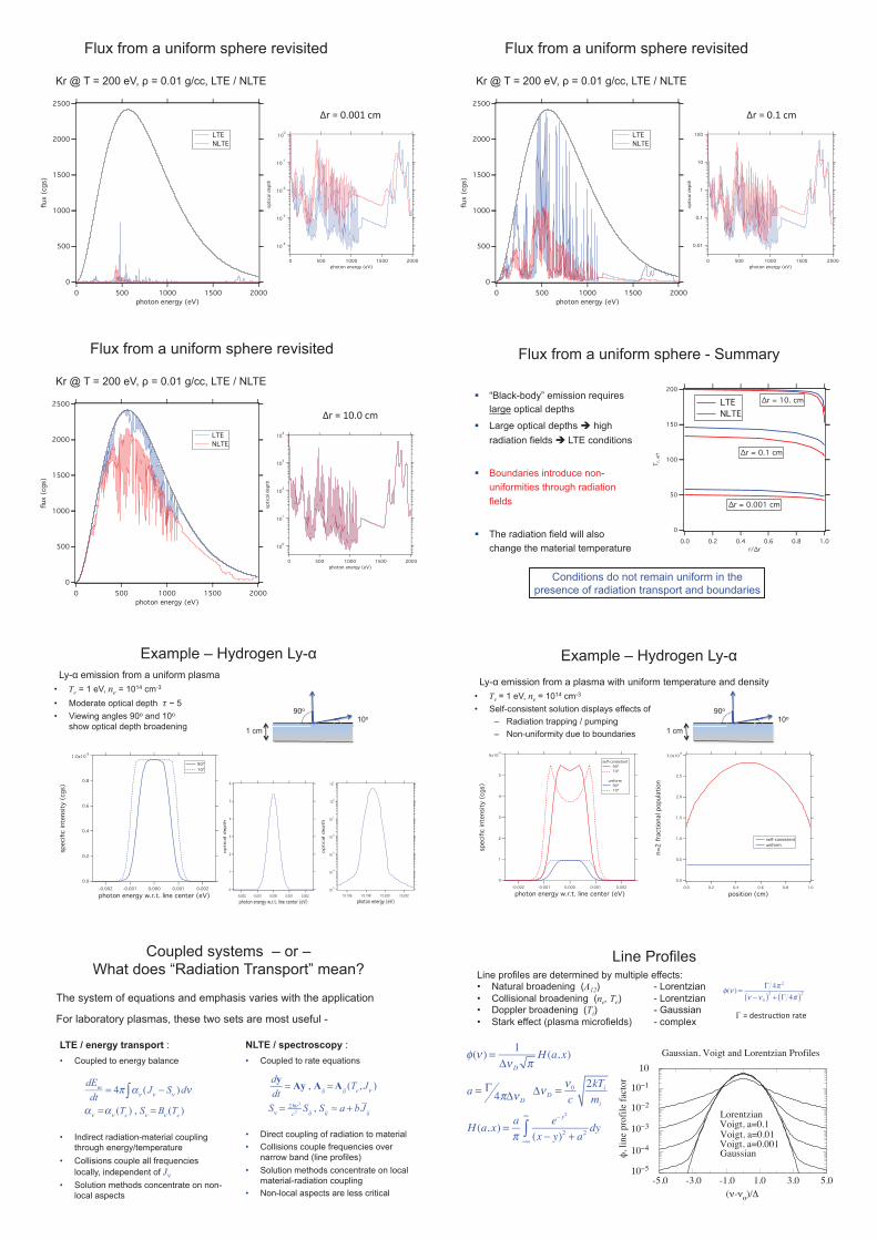
Flux from a uniform sphere revisited

Kr @ T = 200 eV, ρ = 0.01 g/cc, LTE / NLTE

=+!>!?@??A!%,!

2500

2000

1500

1000

500

0

flux (

cgs)

2000150010005000

photon energy (eV)

LTE

NLTE

0.01

0.1

1

10

100

opti

cal depth

2000150010005000

photon energy (eV)

Flux from a uniform sphere revisited

Kr @ T = 200 eV, ρ = 0.01 g/cc, LTE / NLTE

=+!>!?@A!%,!

100

101

102

103

104

opti

cal depth

2000150010005000

photon energy (eV)

2500

2000

1500

1000

500

0

flux (

cgs)

2000150010005000

photon energy (eV)

LTE

NLTE

Flux from a uniform sphere revisited

Kr @ T = 200 eV, ρ = 0.01 g/cc, LTE / NLTE

=+!>!A?@?!%,!

Flux from a uniform sphere - Summary

200

150

100

50

0

Tr,

eff

1.00.80.60.40.20.0

r/∆r

LTE

NLTE

∆r = 10. cm

∆r = 0.1 cm

∆r = 0.001 cm

"  “Black-body” emission requires

large optical depths

"  Large optical depths ! high

radiation fields !!LTE conditions

"  Boundaries introduce non-

uniformities through radiation

fields

"  The radiation field will also

change the material temperature

Conditions do not remain uniform in the

presence of radiation transport and boundaries

1.0x10-9

0.8

0.6

0.4

0.2

0.0

specifi

c inte

nsi

ty (

cgs)

-0.002 -0.001 0.000 0.001 0.002

photon energy w.r.t. line center (eV)

90º

10º

10-5

10-4

10-3

10-2

10-1

100

101

optic

al depth

10.20210.20010.19810.196

photon energy (eV)

Ly-α emission from a uniform plasma

•  Te = 1 eV, ne = 1014 cm-3

•  Moderate optical depth τ ~ 5

•  Viewing angles 90o and 10o

show optical depth broadening

6

5

4

3

2

1

0

optic

al depth

-0.002 -0.001 0.000 0.001 0.002

photon energy w.r.t. line center (eV)

90o!10o!

1 cm!

Example – Hydrogen Ly-α

3.0x10-8

2.5

2.0

1.5

1.0

0.5

0.0

n=

2 f

racti

onal popula

tion

1.00.80.60.40.20.0

position (cm)

self-consistent

uniform

6x10-9

5

4

3

2

1

0

specifi

c inte

nsi

ty (

cgs)

-0.002 -0.001 0.000 0.001 0.002

photon energy w.r.t. line center (eV)

self-consistent

90º

10º

uniform

90º

10º

Example – Hydrogen Ly-α

Ly-α emission from a plasma with uniform temperature and density

•  Te!= 1 eV, ne!= 1014 cm-3

•  Self-consistent solution displays effects of

–  Radiation trapping / pumping

–  Non-uniformity due to boundaries

and d

90o!10o!

1 cm!

Coupled systems – or –

What does “Radiation Transport” mean?

The system of equations and emphasis varies with the application

For laboratory plasmas, these two sets are most useful -

LTE / energy transport :

•  Coupled to energy balance

•  Indirect radiation-material coupling

through energy/temperature

•  Collisions couple all frequencies

locally, independent of Jν

•  Solution methods concentrate on non-

local aspects

dEm

dt= 4π α

ν(J

ν− S

ν)∫ dν

αν=α

ν(T

e) , S

ν= B

ν(T

e)

NLTE / spectroscopy :

•  Coupled to rate equations

•  Direct coupling of radiation to material

•  Collisions couple frequencies over

narrow band (line profiles)

•  Solution methods concentrate on local

material-radiation coupling

•  Non-local aspects are less critical

dy

dt= Ay , A

ij=A

ij(T

e, J

ν)

Sν=

2hν3

c2 Sij

, Sij≈ a + b J

ij

Line Profiles

Line profiles are determined by multiple effects: •  Natural broadening (A12) - Lorentzian

•  Collisional broadening (ne, Te) - Lorentzian •  Doppler broadening (Ti) - Gaussian

•  Stark effect (plasma microfields) - complex

-5.0 -3.0 -1.0 1.0 3.0 5.0

, li

ne

pro

file

fac

tor

Gaussian, Voigt and Lorentzian Profiles

Gaussian

Lorentzian

Voigt, a=0.001Voigt, a=0.01Voigt, a=0.1

( - o)/

!"

!" !

!" #

!" $

!" %

!" &

φ(ν ) =1

∆νD πH (a, x)

a = Γ4π∆νD

∆νD =ν0

c

2kTi

mi

H (a, x) =a

πe− y2

(x − y)2 + a2−∞

∞

∫ dy

φ(ν ) =Γ 4π 2

ν −ν0( )2

+ Γ 4π( )2

Γ >!-*9;+3%8$/!+&;*!

Redistribution

The emission profile is determined by multiple effects: •  collisional excitation ! natural line profile (Lorentzian)

•  photo excitation + coherent scattering •  photo excitation + elastic scattering ! ~absorption profile

•  Doppler broadening

This is described by the redistribution function

Complete redistribution (CRD):

Doppler broadening is only slightly different from CRD, while coherent scattering gives

A good approximation for partial redistribution (PRD) is often

where f (<<1 for X-rays) is the ratio of elastic scattering and de-excitation

rates, includes coherent scattering and Doppler broadening

ψ ν = φν

ψ ν

R(ν , ′ν )

R(ν , ′ν )0

∞

∫ dv = φ( ′ν ) , ψ (ν ) = R(ν , ′ν )0

∞

∫ J ( ′ν )d ′v φ( ′ν )0

∞

∫ J ( ′ν )d ′v

R(ν , ′ν ) = φ(ν )δ (ν − ′ν )

R(ν , ′ν ) = (1− f )φ( ′ν )φ(ν )+ f R

II(ν , ′ν )

R

II

6x10-9

5

4

3

2

1

0

specifi

c inte

nsi

ty (

cgs)

-0.002 -0.001 0.000 0.001 0.002

photon energy w.r.t. line center (eV)

PRD

90º

10º

CRD

90º

10º

uniform

90º

10º

3.5x10-8

3.0

2.5

2.0

1.5

1.0

0.5

0.0

n=

2 f

racti

onal popula

tion

1.00.80.60.40.20.0

position (cm)

PRD

CRD

uniform

Hydrogen Ly-α w/ Partial Redistribution

90o!10o!

1 cm!

Ly-α emission from a plasma with uniform temperature and density

•  Te!= 1 eV, ne!= 1014 cm-3

•  Optical depth τ ~ 5

•  Voigt parameter a ~ 0.0003

Material Velocity

The discussion so far applies in the reference frame of the material

Doppler shifts matter for line radiation when v/c ~ ∆E/E

If velocity gradients are present, either

a)  Transform the RTE into the co-moving frame - or –

b)  Transform material properties into the laboratory frame

Option (a) is complicated (particularly when v/c ! 1)

- see the references by Castor and Mihalas for discussions

Option (b) is relatively simple, but makes the absorption and

emission coefficients direction-dependent

Al sphere w/ uniform expansion velocity

10-5

10-4

10-3

10-2

10-1

100

101

102

opti

cal depth

240022002000180016001400

photon energy (eV)

0.1

1

10

100

are

al flux (

erg

/s/

Hz/st

er)

240022002000180016001400

photon energy (eV)

v/c = 0

v/c = 0.003

v/c = 0.01

v/c = 0.03

optical depth areal flux

uni

(*!>!H??!*I!

!J!>!A?6K!FL%,K!

M$3;*+!>!A@?!%,!

M0//*+!>!?@N!%,!

0.1

1

10

100

are

al flux (

erg

/s/

Hz/st

er)

1800170016001500

photon energy (eV)

v/c = 0

v/c = 0.003

v/c = 0.01

v/c = 0.03

Al sphere w/ uniform expansion velocity

He-α Ly-α

2-Level Atom

Rate equation for two levels in steady state:

Absorption / Emission:

Source Function:

2 g2

1

n2

g1

n1

Two energy level systemn1(B

12J12+C

12) = n

2(A

21+ B

21J12+C

21)

J

12= J

v0

∞

∫ φ12

v( )dv , C12=

g2

g1

e−hν

0kT

C21

∆E = hv0

αν =hν

4πn1B12− n

2B21( )φ12 (ν ) , ην =

hν

4πn2A21φ12(ν )

Sν=n2A21

n1B12− n

2B21

= (1− ε )J12+ εB

ν,

ε

1− ε=C21

A21

1− e−hν0 kT( )

Sν is independent of frequency and linear in

- solution methods exploit this dependence

J

A Popular Solution Technique

For a single line, the system of equations can be expressed as

where the lambda operator and the source function depend on the

populations through the absorption and emission coefficients.

A numerical solution for uniquely specifies the entire system.

Since depends on through the populations, the full system is

non-linear and requires iterating solutions of the rate equations and

radiation transport equation.

The dependence of on is usually weak, so convergence is rapid.

dIv

dτv

= − Iv+ S

v⇒ I

v=!

λνSv(J )

Sv= aν + bν J , J =

1

4πdΩ∫ I

v0

∞

∫ φ v( )dv

!

λν

J

J

J

!

λν

!

λν

Solution technique for the linear source function:

This linear system can (in principle) be solved directly for

and in 1D this is very efficient

The (angle,frequency)-integrated operator includes

factors, so amplifies (radiation trapping)

Efficient solution methods approximate key parts of

NLTE – local frequency scattering

LTE (linear in ∆Te) – non-local coupling

Iv=!

λν aν + bν J

⇒ J =1

4πdΩ∫

!

λν aν + bν J 0

∞

∫ φ v( )dv

⇒ J = 1−!Λ

−1 1

4πdΩ∫

!

λνaν0

∞

∫ φ v( )dv

!Λ =

1

4πdΩ∫

!

λνbν0

∞

∫ φ v( )dv

J

J

!Λ

1−!Λ

−1

1− e−τν

!Λ

For multiple lines, the source function for each line can be put in the

two-level form – ETLA (Extended Two Level Atom) – or the full

source function can be expressed in the following manner:

Solve for each individually (if coupling between lines is not

important) or simultaneously.

(Complete) linearization – expand in terms of

and solve as before.

Partial redistribution usually converges at a slightly slower rate.

Jℓ

Sv=

ην

c+ η

ν

ℓ(Jℓ)φ

ν

ℓ

ℓ

∑

αν

c+ α

ν

ℓ(Jℓ)φ

ν

ℓ

ℓ

∑

Multi-Level Atom

Sν

∆Jℓ

Sν =Sν (Jℓ0)+

∂Sν

∂Jℓ

Jℓ− J

ℓ

0( )ℓ

∑

Numerical methods need to fulfill 2 requirements

1.  Accurate formal transport solution which is

•  conservative,

•  non-negative

•  2nd order (spatial) accuracy (diffusion limit as τ >> 1)

•  causal (+ efficient)

Many options are available – each has advantages and disadvantages

2. Method to converge solution of coupled implicit equations

•  Multiple methods fall into a few classes

–  Full nonlinear system solution

–  Accelerated transport solution

–  Incorporate transport information into other physics

•  Optimized methods are available for specific regimes, but no single

method works well across all regimes

Method #1 – Source (or lambda) iteration

Advantages –

Simple to implement

Independent of formal transport method

Disadvantages –

Can require many iterations: # iterations ~ τ2

False convergence is a problem for τ >> 1

1.  Evaluate source function

2.  Formal solution of radiation

transport equation

3.  Use intensities to evaluate

temperature / populations

source function

olution of radiation

t equation

nsities to evaluate

ure / populations

sou sou

0;*+&;*!;$!

%$/:*+F*/%*!

Hydrogen Lyman-α revisited

•  Source iteration (green curves) approaches self-consistent solution slowly

•  Linearization achieves convergence in 1 iteration

S

ij= a + b J

ij, J

ij= Jνφv

dν∫ #!'0/*&+!B3/%8$/!$B!

3.0x10-8

2.5

2.0

1.5

1.0

0.5

0.0

n=

2 f

racti

onal popula

tion

1.00.80.60.40.20.0

position (cm)

self-consistent

uniform

6x10-9

5

4

3

2

1

0

specifi

c inte

nsi

ty (

cgs)

-0.002 -0.001 0.000 0.001 0.002

photon energy w.r.t. line center (eV)

90º

self-consistent

uniform

0;*+&8$/!O!

0;*+&8$/!O!

J

Method #2 – Monte Carlo

Formal solution method –

1)  Sample emission distribution in (space, frequency, direction) to create “photons”

2)  Track “photons” until they escape or are destroyed

Advantages –

Works well for complicated geometries

Not overly constrained by discretizations ! does details very well

Disadvantages –

Statistical noise improves slowly with # of particles

Expense increases with optical depth

Iterative evaluation of coupled system is not possible / advisable

Semi-implicit nature requires careful timestep control

Convergence –

A procedure that transforms absorption/emission events into effective

scatterings (Implicit Monte Carlo) provides a semi-implicit solution

Symbolic IMC provides a fully-implicit solution at the cost of a solving a

single mesh-wide nonlinear equation

Method #3 – Discrete Ordinates (SN)

Formal solution method –

Discretization in angle converts integro-differential equations into a set of coupled

differential equations (provides lambda operator)

Advantages –

Handles regions with τ<<1 and τ>>1 equally well

Modern spatial discretizations achieve the diffusion limit

Deterministic method can be iterated to convergence

Disadvantages –

Ray effects due to preferred directions

angular profiles become inaccurate well before angular integrals

Required # of angles in 2D/3D can become enormous

Discretization in 7 dimensions requires large computational resources

Convergence –

Effective solution algorithms exist for both LTE and NLTE versions [6] –

e.g. LTE – synthetic grey transport (or diffusion)

NLTE – complete linearization (provides linear source function)

+ accelerated lambda iteration in 2D/3D

(Note: this applies to all deterministic methods)

Method #4 – Escape factors

Escape factor pe is used to eliminate radiation field from net radiative rate

Equivalent to incorporating a (partial) lambda operator into the rate equations

! combines the formal solution + convergence method

Advantages –

Very fast – no transport equation solution required Can be combined with other physics with no (or minimal) changes

Disadvantages – Details of transport solution are absent

Escape factors depend on line profiles, system geometry Iterative improvement is possible, but usually not worthwhile

y jBjiJ − yiBijJ = y jAji pe

Escape factor is built off the single flight escape probability Iron’s theorem – this gives the correct rate on average

(spatial average weighted by emission) Note that the optical depth depends on the line profile, plus continuum Asymptotic expressions for large optical depth:

Gaussian profile Voigt profile Evaluating pe can be complicated by overlapping lines, Doppler shifts, etc. Many variations and extensions exist in a large literature

p

e=

1

4πdΩ∫ e

−τν

0

∞

∫ φ v( )dv

1− JS

= pe

e−τν

pe≈1 4τ ln τ π( ) p

e≈ 1

3a τ

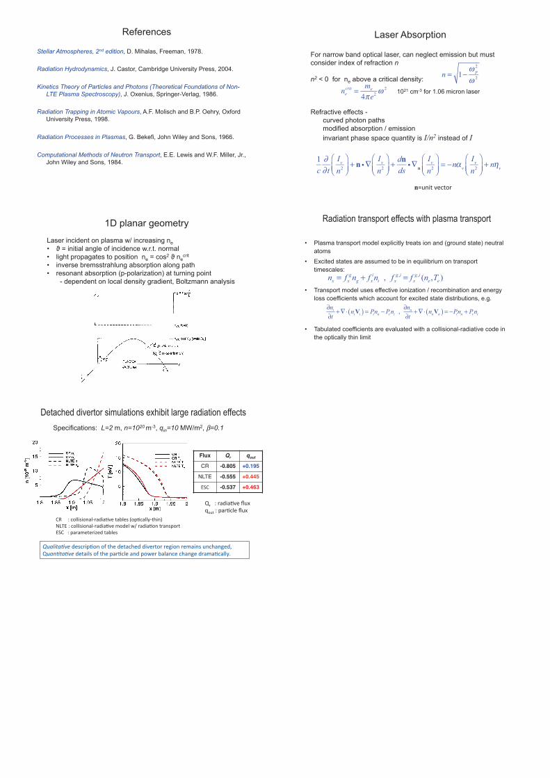
References

Stellar Atmospheres, 2nd edition, D. Mihalas, Freeman, 1978.

Radiation Hydrodynamics, J. Castor, Cambridge University Press, 2004.

Kinetics Theory of Particles and Photons (Theoretical Foundations of Non-

LTE Plasma Spectroscopy), J. Oxenius, Springer-Verlag, 1986.

Radiation Trapping in Atomic Vapours, A.F. Molisch and B.P. Oehry, Oxford

University Press, 1998.

Radiation Processes in Plasmas, G. Bekefi, John Wiley and Sons, 1966.

Computational Methods of Neutron Transport, E.E. Lewis and W.F. Miller, Jr.,

John Wiley and Sons, 1984.

Laser Absorption

For narrow band optical laser, can neglect emission but must

consider index of refraction n

n2 < 0 for ne above a critical density:

Refractive effects -

curved photon paths

modified absorption / emission

invariant phase space quantity is I/n2 instead of I

ne

crit=

me

4πe2ω

2

1

c

∂∂ t

Iv

n2

+ n i∇

Iv

n2

+

dn

dsi∇

n

Iv

n2

= −nα

v

Iv

n2

+ nη

v

n = 1−ω

p

2

ω2

1021 cm-3 for 1.06 micron laser!

n>3/0;!:*%;$+!

1D planar geometry

Laser incident on plasma w/ increasing ne

•  ϑ = initial angle of incidence w.r.t. normal

•  light propagates to position ne = cos2 ϑ necrit

•  inverse bremsstrahlung absorption along path

•  resonant absorption (p-polarization) at turning point

- dependent on local density gradient, Boltzmann analysis

Radiation transport effects with plasma transport

•  Plasma transport model explicitly treats ion and (ground state) neutral

atoms

•  Excited states are assumed to be in equilibrium on transport

timescales:

•  Transport model uses effective ionization / recombination and energy

loss coefficients which account for excited state distributions, e.g.

•  Tabulated coefficients are evaluated with a collisional-radiative code in

the optically thin limit

, ,, ( , )g i g i g i

x x g x i x x e en f n f n f f n T= + =

( ) ( ),i n

i i i n r i n n i n r i

n nn Pn Pn n Pn Pn

t t

∂ ∂+∇⋅ = − +∇⋅ = − +

∂ ∂V V

Detached divertor simulations exhibit large radiation effects

Specifications: L=2 m, n=1020 m-3, qin=10 MW/m2, β=0.1

!"#$%&#'()!-*9%+078$/!$B!;)*!-*;&%)*-!-0:*+;$+!+*F0$/!+*,&0/9!3/%)&/F*-<!

P"#*'&#'()!-*;&0'9!$B!;)*!7&+8%'*!&/-!7$Q*+!4&'&/%*!%)&/F*!-+&,&8%&''.@!

RM!!!!!S!%$''090$/&'6+&-0&8:*!;&4'*9!"$78%&''.6;)0/5!

T#(1!S!%$''090$/&'6+&-0&8:*!,$-*'!QL!+&-0&8$/!;+&/97$+;!

1UR!!!S!7&+&,*;*+0V*-!;&4'*9!

Flux Qr qout

CR -0.805 +0.195

NLTE -0.555 +0.445

1UR! -0.537 +0.463

P+!!!S!+&-0&8:*!W3X!

2$3;!S!7&+8%'*!W3X!