Lecture Notes on Modelling and System Identification ... · i i “msi” — 2014/11/26 — 15:16...
39
Lecture Notes on Modelling and System Identification (Preliminary Draft) Moritz Diehl November 26, 2014
Transcript of Lecture Notes on Modelling and System Identification ... · i i “msi” — 2014/11/26 — 15:16...
ii
“msi” — 2014/11/26 — 15:16 — page 1 — #1 ii
ii
ii
Lecture Notes on Modelling and System Identification(Preliminary Draft)
Moritz Diehl
November 26, 2014

ii
“msi” — 2014/11/26 — 15:16 — page 2 — #2 ii
ii
ii
2
ii
“msi” — 2014/11/26 — 15:16 — page 3 — #3 ii
ii
ii
Contents
Preface 5
1 Introduction 71.1 Mathematical Notation . . . . . . . . . . . . . . . . . . . . . . . . . . . . . . . . . . . . . . . . 71.2 A Simple Example: Resistance Estimation . . . . . . . . . . . . . . . . . . . . . . . . . . . . . . 8
2 Probability and Statistics in a Nutshell 112.1 Random Variables and Probabilities . . . . . . . . . . . . . . . . . . . . . . . . . . . . . . . . . 112.2 Scalar Random Variables and Probability Density Functions . . . . . . . . . . . . . . . . . . . . 112.3 Multidimensional Random Variables . . . . . . . . . . . . . . . . . . . . . . . . . . . . . . . . . 122.4 Statistical Estimators . . . . . . . . . . . . . . . . . . . . . . . . . . . . . . . . . . . . . . . . . 132.5 Analysis of the Resistance Estimation Example . . . . . . . . . . . . . . . . . . . . . . . . . . . 14
3 Linear Least Squares Estimation 153.1 Least Squares Problem Formulation . . . . . . . . . . . . . . . . . . . . . . . . . . . . . . . . . 153.2 A Micro-Review of Unconstrained Optimization . . . . . . . . . . . . . . . . . . . . . . . . . . . 163.3 Solution of the Linear Least Squares Problem . . . . . . . . . . . . . . . . . . . . . . . . . . . . 173.4 Weighted Least Squares . . . . . . . . . . . . . . . . . . . . . . . . . . . . . . . . . . . . . . . . 183.5 Ill-Posed Least Squares and the Moore Penrose Pseudo Inverse . . . . . . . . . . . . . . . . . . . 193.6 Statistical Analysis of the Weighted Least Squares Estimator . . . . . . . . . . . . . . . . . . . . 223.7 Measuring the Goodness of Fit using R-Squared . . . . . . . . . . . . . . . . . . . . . . . . . . . 233.8 Estimating the Covariance with a Single Experiment . . . . . . . . . . . . . . . . . . . . . . . . 23
4 Maximum Likelihood and Bayesian Estimation 274.1 Maximum Likelihood Estimation . . . . . . . . . . . . . . . . . . . . . . . . . . . . . . . . . . . 274.2 Bayesian Estimation and the Maximum A Posteriori Estimate . . . . . . . . . . . . . . . . . . . . 284.3 Recursive Linear Least Squares . . . . . . . . . . . . . . . . . . . . . . . . . . . . . . . . . . . . 28
5 Dynamic Systems in a Nutshell 295.1 Dynamic System Classes . . . . . . . . . . . . . . . . . . . . . . . . . . . . . . . . . . . . . . . 295.2 Continuous Time Systems . . . . . . . . . . . . . . . . . . . . . . . . . . . . . . . . . . . . . . 315.3 Discrete Time Systems . . . . . . . . . . . . . . . . . . . . . . . . . . . . . . . . . . . . . . . . 355.4 Input Output Models . . . . . . . . . . . . . . . . . . . . . . . . . . . . . . . . . . . . . . . . . 37
3

ii
“msi” — 2014/11/26 — 15:16 — page 4 — #4 ii
ii
ii
4 CONTENTS
ii
“msi” — 2014/11/26 — 15:16 — page 5 — #5 ii
ii
ii
Preface to the Preliminary Manuscript
This lecture manuscript is written to accompany a lecture course on “Modelling and System Identification” given inthe winter term 2014/15 at the University of Freiburg. Some parts and figures are based on a previous manuscriptfrom the same course a year earlier, which was compiled by Benjamin Volker, and on the lecture notes from acourse on numerical optimization the author has previously taught at the University of Leuven. Aim of the presentmanuscript is that it shall serve to the students as a reference for study during the semester. It follows the generalstructure of the lecture course and is written during the semester. The current version is a preliminary version only.A complete version shall be finalized in the weeks after the end of the semester, such that the final script can beused for exam preparation.
Freiburg, November 2014 -February 2015 Moritz Diehl
5

ii
“msi” — 2014/11/26 — 15:16 — page 6 — #6 ii
ii
ii
6 CONTENTS
ii
“msi” — 2014/11/26 — 15:16 — page 7 — #7 ii
ii
ii
Chapter 1
Introduction
The lecture course on Modelling and System Identification (MSI) has as its aim to enable the students to createmodels that help to predict the behaviour of systems. Here, we are particularly interested in dynamic systemmodels, i.e. systems evolving in time. With good system models, one can not only predict the future (like inweather forecasting), but also control or optimize the behaviour of a technical system, via feedback control orsmart input design. Having a good model gives us access to powerful engineering tools. This course focuseson the process to obtain such models. It builds on knowledge from three fields: Systems Theory, Statistics, andOptimization. We will recall necessary concepts from these three fields on demand during the course. For amotivation for the importance of statistics in system identification, we first look at a very simple example takenfrom the excellent lecture notes of J. Schoukens [Sch13]. The course will then first focus on identification methodsfor static models and their statistical properties, and review the necessary concepts from statistics and optimizationwhere needed. Later, we will look at different ways to model dynamic systems and how to identify them. For amuch more detailed and complete treatment of system identification, we refer to the textbook by L. Ljung [Lju99].
1.1 Mathematical NotationWithin this lecture we use R for the set of real numbers, R+ for the non-negative ones and R++ for the positiveones, Z for the set of integers, and N for the set of natural numbers including zero, i.e. we identify N = Z+. Theset of real-valued vectors of dimension n is denoted by Rn, and Rn×m denotes the set of matrices with n rows andm columns. By default, all vectors are assumed to be column vectors, i.e. we identify Rn = Rn×1. We usually usesquare brackets when presenting vectors and matrices elementwise. Because will often deal with concatenations ofseveral vectors, say x ∈ Rn and y ∈ Rm, yielding a vector in Rn+m, we abbreviate this concatenation sometimesas (x, y) in the text, instead of the correct but more clumsy equivalent notations [x>, y>]> or[
xy
].
Square and round brackets are also used in a very different context, namely for intervals in R, where for two realnumbers a < b the expression [a, b] ⊂ R denotes the closed interval containing both boundaries a and b, while anopen boundary is denoted by a round bracket, e.g. (a, b) denotes the open interval and [a, b) the half open intervalcontaining a but not b.
When dealing with norms of vectors x ∈ Rn, we denote by ‖x‖ an arbitrary norm, and by ‖x‖2 the Euclideannorm, i.e. we have ‖x‖22 = x>x. We denote a weighted Euclidean norm with a positive definite weighting matrixQ ∈ Rn×n by ‖x‖Q, i.e. we have ‖x‖2Q = x>Qx. The L1 and L∞ norms are defined by ‖x‖1 =
∑ni=1 |xi|
and ‖x‖∞ = max{|x1|, . . . , |xn|}. Matrix norms are the induced operator norms, if not stated otherwise, and theFrobenius norm ‖A‖F of a matrix A ∈ Rn×m is defined by ‖A‖2F = trace(AA>) =
∑ni=1
∑mj=1AijAij .
When we deal with derivatives of functions f with several real inputs and several real outputs, i.e. functionsf : Rn → Rm, x 7→ f(x), we define the Jacobian matrix ∂f
∂x (x) as a matrix in Rm×n, following standardconventions. For scalar functions with m = 1, we denote the gradient vector as ∇f(x) ∈ Rn, a column vector,also following standard conventions. Slightly less standard, we generalize the gradient symbol to all functionsf : Rn → Rm even with m > 1, i.e. we generally define in this lecture
∇f(x) =∂f
∂x(x)> ∈ Rn×m.
7
ii
“msi” — 2014/11/26 — 15:16 — page 8 — #8 ii
ii
ii
8 CHAPTER 1. INTRODUCTION
Using this notation, the first order Taylor series is e.g. written as
f(x) = f(x) +∇f(x)>(x− x)) + o(‖x− x‖)
The second derivative, or Hessian matrix will only be defined for scalar functions f : Rn → R and be denoted by∇2f(x).
For square symmetric matrices of dimension n we sometimes use the symbol Sn, i.e. Sn = {A ∈ Rn×n|A =A>}. For any symmetric matrixA ∈ Sn we writeA<0 if it is a positive semi-definite matrix, i.e. all its eigenvaluesare larger or equal to zero, and A�0 if it is positive definite, i.e. all its eigenvalues are positive. This notation isalso used for matrix inequalities that allow us to compare two symmetric matrices A,B ∈ Sn, where we definefor example A<B by A−B<0.
When using logical symbols, A⇒ B is used when a propositionA implies a propositionB. In words the sameis expressed by “If A then B”. We write A⇔ B for “A if and only if B”, and we sometimes shorten this to “A iffB”, with a double “f”, following standard practice.
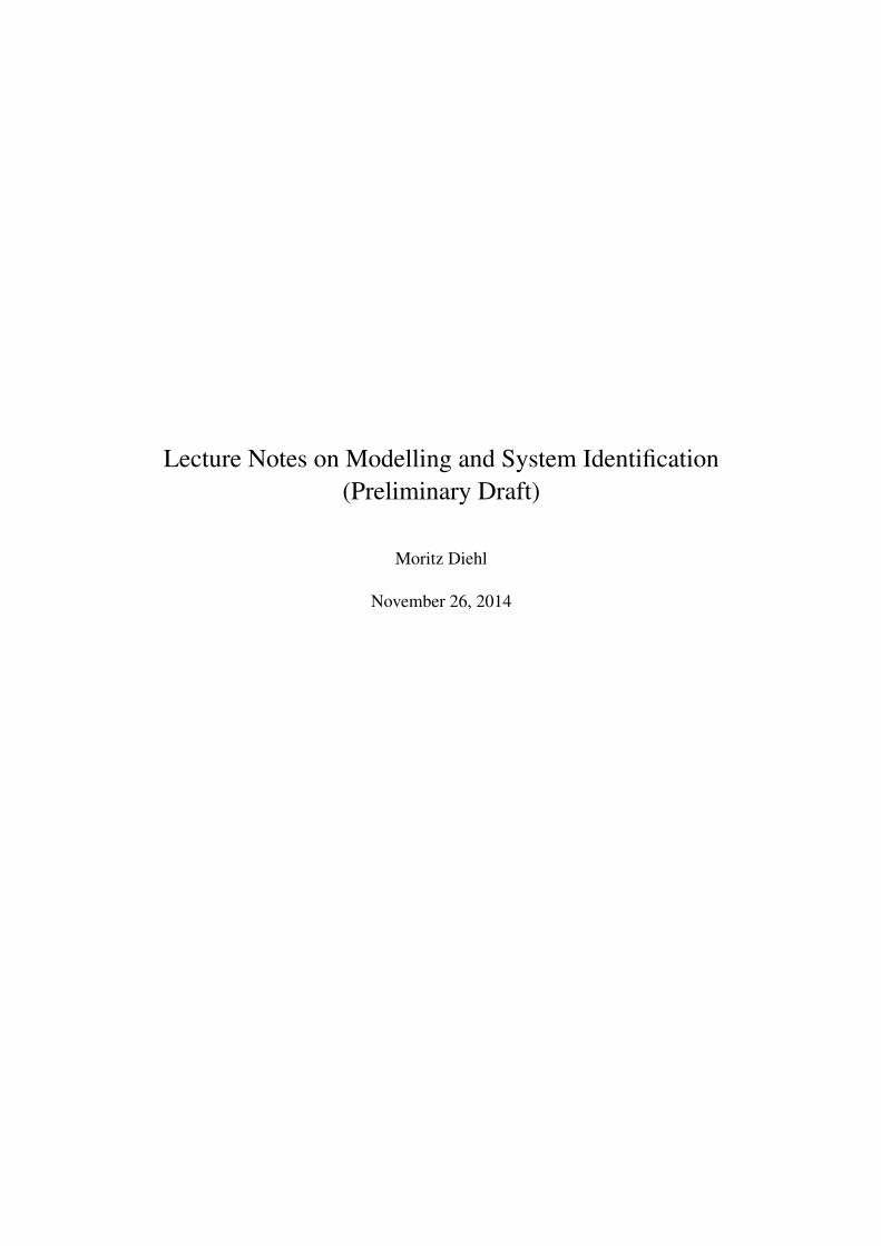
1.2 A Simple Example: Resistance EstimationCHAPTER 1. AN INTRODUCTION TO IDENTIFICATION
Figure 1.1: Measurement of a resistor.
0
5
0 50 100
Mea
sure
d va
lue
R (O
hm)
Measurement number
0
2
0 50 100
Volta
ge (V
)
Measurement number
0
2
0 50 100
Curre
nt (A
)
Measurement number(a) Group A
0
5
0 50 100
Mea
sure
d va
lue
R (O
hm)
Measurement number
0
2
0 50 100
Volta
ge (V
)
Measurement number
0
2
0 50 100
Curre
nt (A
)
Measurement number(b) Group B
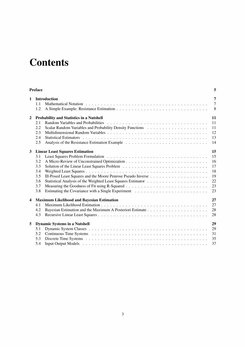
Figure 1.2: Measurement results u(k), i(k) for groups A and B.The plotted value R(k) is obtained by direct division of the voltage by thecurrent: R(k) = u(k)/i(k).
The index N indicates that the estimate is based on N observations. Note
that the three estimators result in the same estimate on noiseless data. Both
groups processed their measurements and their results are given in Figure 1.3.
From this figure a number of interesting observations can be made:
10
Figure 1.1: Resistance estimation example with resistorR , current measurements i(k), and voltage measurementsu(k) for k = 1, 2, ...., N. [Sch13]
3
i(k)/A
k1 N2 3
u(k)/V
k1 N2
u(k)/V
i(k)/A
+ +
+
++
+
+
++ +
u(k)/V
i(k)/A
++ R·i(k)
u(k)
f(R)
RRLS
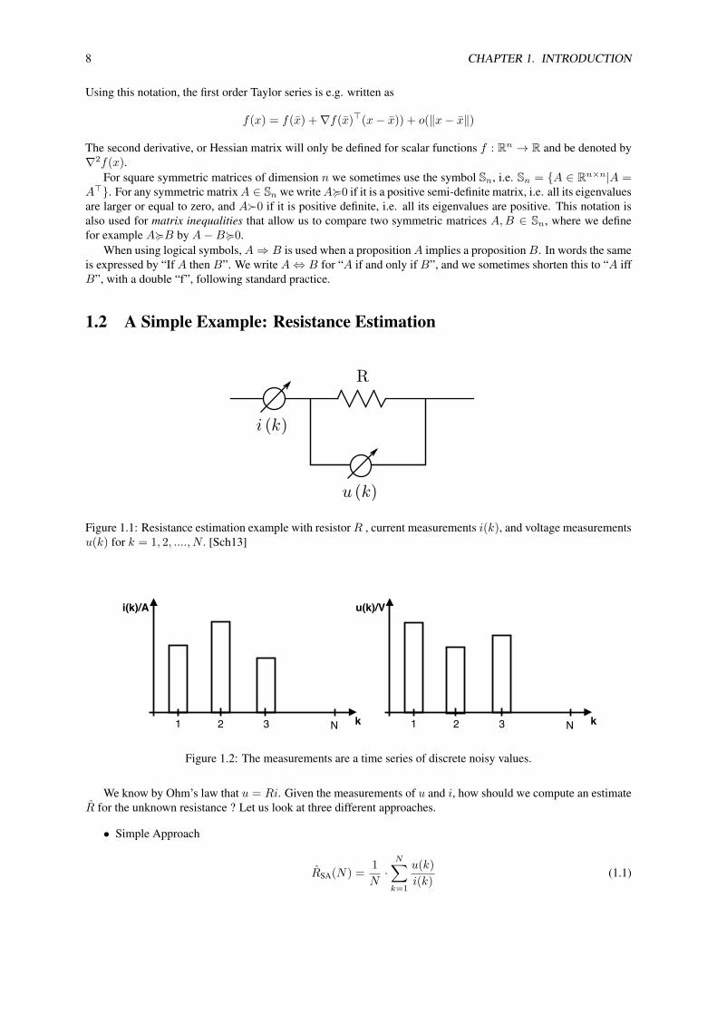
Figure 1.2: The measurements are a time series of discrete noisy values.
We know by Ohm’s law that u = Ri. Given the measurements of u and i, how should we compute an estimateR for the unknown resistance ? Let us look at three different approaches.
• Simple Approach
RSA(N) =1
N·N∑k=1
u(k)
i(k)(1.1)
ii
“msi” — 2014/11/26 — 15:16 — page 9 — #9 ii
ii
ii
1.2. A SIMPLE EXAMPLE: RESISTANCE ESTIMATION 9
3
i(k)/A
k1 N2 3
u(k)/V
k1 N2
u(k)/V
i(k)/A
+ +
+
++
+
+
++ +
u(k)/V
i(k)/A
++ R·i(k)
u(k)
f(R)
RRLS
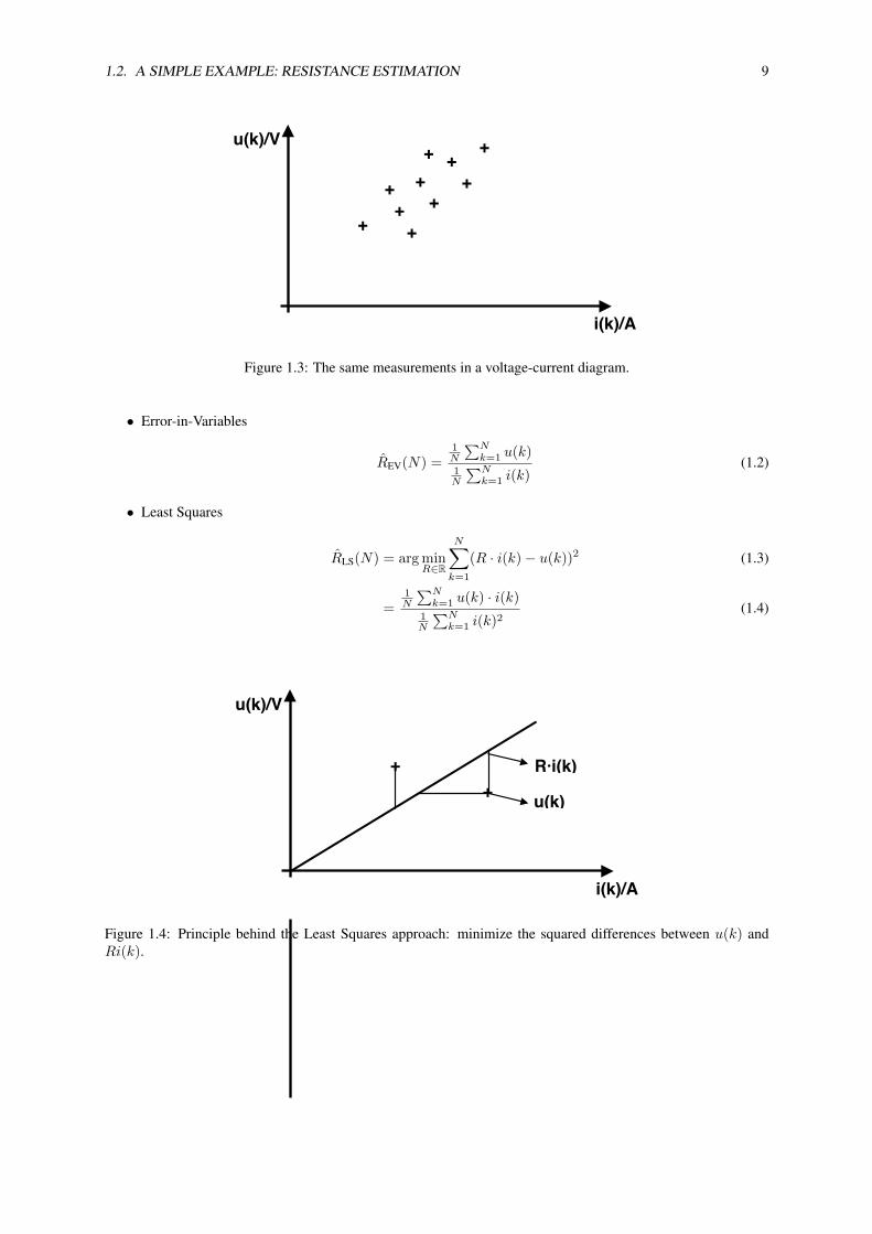
Figure 1.3: The same measurements in a voltage-current diagram.
• Error-in-Variables
REV(N) =1N
∑Nk=1 u(k)
1N
∑Nk=1 i(k)
(1.2)
• Least Squares
RLS(N) = arg minR∈R
N∑k=1
(R · i(k)− u(k))2 (1.3)
=1N
∑Nk=1 u(k) · i(k)
1N
∑Nk=1 i(k)2
(1.4)
3
i(k)/A
k1 N2 3
u(k)/V
k1 N2
u(k)/V
i(k)/A
+ +
+
++
+
+
++ +
u(k)/V
i(k)/A
++ R·i(k)
u(k)
f(R)
RRLS
Figure 1.4: Principle behind the Least Squares approach: minimize the squared differences between u(k) andRi(k).
ii
“msi” — 2014/11/26 — 15:16 — page 10 — #10 ii
ii
ii
10 CHAPTER 1. INTRODUCTION
CHAPTER 1. AN INTRODUCTION TO IDENTIFICATION
0
1
2
1 10 100 1000 10000
R(N
)(O
hm)
N
0
1
2
1 10 100 1000 10000
R(N
)(O
hm)
N
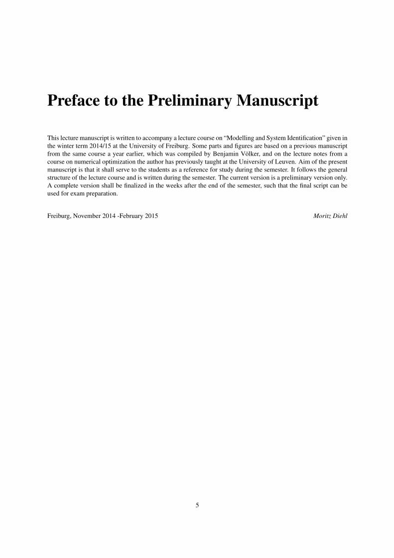
Figure 1.3: Estimated resistance values R(N) for both groups as a function ofthe number of processed data N .
Full dotted line: RSA, dotted line: RLS, full line: REV.
• All estimators have large variations for small values of N , and seem to
converge to an asymptotic value for large values of N , except RSA(N) of
group A. This corresponds to the intuitively expected behavior: if a large
number of data points are processed we should be able to eliminate the
noise influence due to the averaging effect.
• The asymptotic values of the estimators depend on the kind of averaging
technique that is used. This shows that there is a serious problem: at least
2 out of the 3 methods converge to a wrong value. It is not even certain
that any one of the estimators is doing well. This is quite catastrophic:
even an infinite amount of measurements does not guarantee that the
exact value is found.
• The RSA(N) of group A behaves very strangely. Instead of converging
to a fixed value, it jumps irregularly up and down before convergence is
reached.
These observations prove very clearly that a good theory is needed to explain
and understand the behavior of candidate estimators. This will allows us to
make a sound selection out of many possibilities and to indicate in advance,
11
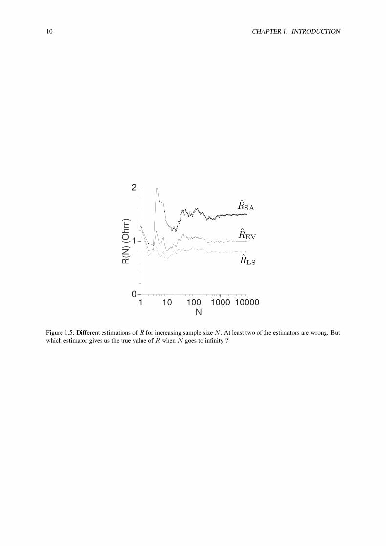
Figure 1.5: Different estimations of R for increasing sample size N . At least two of the estimators are wrong. Butwhich estimator gives us the true value of R when N goes to infinity ?

ii
“msi” — 2014/11/26 — 15:16 — page 11 — #11 ii
ii
ii
Chapter 2
Probability and Statistics in a Nutshell
In this chapter we review concepts from the fields of mathematical statistics and probability that we will need oftenin this course.
2.1 Random Variables and ProbabilitiesRandom variables are used to describe the possible outcomes of experiments. Random variables are slightlydifferent than the usual mathematical variables, because a random variable does not yet have a value. A randomvariable X can take values from a given set, typically the real numbers. A specific value x ∈ R of the randomvariableX will typically be denoted by a lower case letter, while the random variable itself will usually be denotedby an upper case letter; we will mostly, but not always stick to this convention. Note that the random variableX itself is not a real number, but just takes values in R. Nevertheless, we sometimes write sloppily X ∈ R, orY ∈ Rn to quickly indicate that a random variable takes scalars or vectors as values.
The probability that a certain event A occurs is denoted by P (A), and P (A) is a real number in the interval[0, 1]. The event A is typically defined by a condition that a random variable can satisfy or not. For example, theprobability that the value of a random variable X is larger than a fixed number a is denoted by P (X > a). If theevent contains all possible outcomes of the underlying random variable X , its probability is one. If two events Aand B are mutually exclusive, i.e. are never true at the same time, the probability that one or the other occurs isgiven by the sum of the two probabilities: P (A ∨B) = P (A) + P (B). Two events can also be independent fromeach other. In that case, the probability that they both occur is given by the product: P (A ∧ B) = P (A)P (B). Ifthis is not the case, the two events are called dependent. We will often also write P (A,B) for the joint probabilyP (A ∧ B). One can define the conditional probability P (A|B) that an event A occurs given that event B hasalready occured. It is easy to verify the identity
P (A|B) =P (A,B)
P (B).
An immediate consequence of this identity is
P (A|B) =P (B|A)P (A)
P (B).
which is known as Bayes Theorem after Thomas Bayes (17011761), who investigated how new evidence (event Bhas occured) can update prior beliefs (a-priori probability P (A)).
2.2 Scalar Random Variables and Probability Density FunctionsFor a real valued random variable X , one can define the Probability Density Function (PDF) pX(x) which de-scribes the behaviour of the random variable, and which is a function from the real numbers to the real numbers,i.e. pX : R → R, x 7→ pX(x). Note that we use the name of the underlying random variable (here X) as index,when needed, and that the input argument x of the PDF is just a real number. We will sometimes drop the indexwhen the underlying random variable is clear from the context.
11
ii
“msi” — 2014/11/26 — 15:16 — page 12 — #12 ii
ii
ii
12 CHAPTER 2. PROBABILITY AND STATISTICS IN A NUTSHELL
The PDF pX(x) is related to the probability that X takes values in any interval [a, b] in the following way:
P (X ∈ [a, b]) =
∫ b
a
pX(x) dx
Conversely, one can define the the PDF as
pX(x) = lim∆x→0
P (X ∈ [x, x+ ∆x])
∆x
Two random variables X,Y are independent if the joint PDF pX,Y (x, y) is the product of the individual PDFs, i.e.pX,Y (x, y) = pX(x)pY (y), otherwise they are dependent. The conditional PDF pX|Y of X for given Y is definedby
pX|Y (x|y) =pX,Y (x, y)
pY (y).
As the above notation can become very cumbersome, we will occasionally also omit the index of the PDF and forexample just express the above identity as
p(x|y) =p(x, y)
p(y).
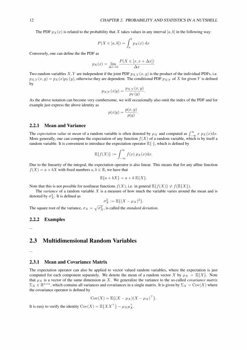
2.2.1 Mean and VarianceThe expectation value or mean of a random variable is often denoted by µX and computed as
∫∞−∞ x pX(x)dx.
More generally, one can compute the expectation of any function f(X) of a random variable, which is by itself arandom variable. It is convenient to introduce the expectation operator E{·}, which is defined by
E{f(X)} :=
∫ ∞−∞
f(x) pX(x)dx.
Due to the linearity of the integral, the expectation operator is also linear. This means that for any affine functionf(X) = a+ bX with fixed numbers a, b ∈ R, we have that
E{a+ bX} = a+ b E{X}.
Note that this is not possible for nonlinear functions f(X), i.e. in general E{f(X)} 6= f(E{X}).The variance of a random variable X is a measure of how much the variable varies around the mean and is
denoted by σ2X . It is defined as
σ2X := E{(X − µX)2}.
The square root of the variance, σX =√σ2X , is called the standard deviation.
2.2.2 Examples...
2.3 Multidimensional Random Variables...
2.3.1 Mean and Covariance MatrixThe expectation operator can also be applied to vector valued random variables, where the expectation is justcomputed for each component separately. We denote the mean of a random vector X by µX = E{X}. Notethat µX is a vector of the same dimension as X . We generalize the variance to the so-called covariance matrixΣX ∈ Rn×n, which contains all variances and covariances in a single matrix. It is given by ΣX = Cov(X) wherethe covariance operator is defined by
Cov(X) = E{(X − µX)(X − µX)>}.
It is easy to verify the identity Cov(X) = E{XX>} − µXµ>X .

ii
“msi” — 2014/11/26 — 15:16 — page 13 — #13 ii
ii
ii
2.4. STATISTICAL ESTIMATORS 13
2.3.2 Multidimensional Normal DistributionWe say that a vector valued random variable X is normally distributed with mean µ and covariance Σ if its PDFp(x) is given by a multidimensional Gaussian as follows
p(x) =1√
det(2πΣ)exp
(−1
2(x− µ)>Σ−1(x− µ)
)As a shorthand, one also writes X ∼ N (µ,Σ) to express that X follows a normal distribution with mean µ andcovariance Σ . One can verify by integral computations that indeed E{X} = µ and Cov(X) = Σ.
2.4 Statistical EstimatorsAn estimator uses possibly many measurements in order to estimate the value of some parameter vector that wetypically denote by θ in this script. The parameter is not random, but its true value, θ0, is not known to the estimator.If we group all the measurements in a vector valued random variable YN ∈ RN , the estimator is a function of YN .We can denote this function by θN (YN ). Due to its dependence on YN , the estimate θN (YN ) is itself a randomvariable, for which we can define mean and covariance. Ideally, the expectation value of the estimator is equal tothe true parameter value θ0. We then say that the estimator is unbiased.
Definition 1 (Biased- and Unbiasedness) An estimator θN is called unbiased iff E{θN (YN )} = θ0, where θ0 isthe true value of a parameter. Otherwise, it is called biased.
Example for unbiasedness: estimating the mean by an average One of the simplest estimators tries to estimatethe mean θ ≡ µY of a scalar random variable Y by averaging N measurements of Y . Each of these measurementsY (k) is random, and overall the random vector YN is given by YN = [Y (1), . . . , Y (N)]>. The estimator θN (YN )is given by
θN (YN ) =1
NΣNk=1Y (k).
It is easy to verify that this estimator is unbiased, because
E{θN (YN )} =1
NΣNk=1E{Y (k)} =
1
NΣNk=1µY = µY
Because this estimator is often used it has a special name. It is called the sample mean.
In order to assess the performance of an unbiased estimator, one can regard the covariance matrix of theestimates, i.e.
Cov(θN (YN ))
The smaller this symmetric positive semi-definite matrix, the better the estimator. If two estimators θA and θB
are both unbiased, and if the matrix inequality Cov(θA)<Cov(θB) holds, we can conclude that the estimator θB
has a better performance than estimator θA. Typically, the covariance of an estimator becomes smaller when anincreasing number N of measurements is used. Often the covariance even tends to zero as N →∞.
Some estimators are not unbiased, but if N tends to infinity, their bias – i.e. the difference between true valueand the mean of the estimate – tends to zero.
Definition 2 (Asymptotic Unbiasedness) An estimator θN is called asymptotically unbiased iff
limN→∞
E{θN (YN )} = θ0.
Example for asymptotically unbiasedness: estimating the variance by the mean squared deviations Oneof the simplest biased, but asymptotically unbiased estimators is tries to estimate the variance θ ≡ σ2
Y of a scalarrandom variable Y by taking N measurements of Y , computing the experimental mean M(YN ) = 1
NΣNk=1Y (k),and then averaging the squared deviations from the mean
θN (YN ) =1
NΣNk=1(Y (k)−M(YN ))2
ii
“msi” — 2014/11/26 — 15:16 — page 14 — #14 ii
ii
ii
14 CHAPTER 2. PROBABILITY AND STATISTICS IN A NUTSHELL
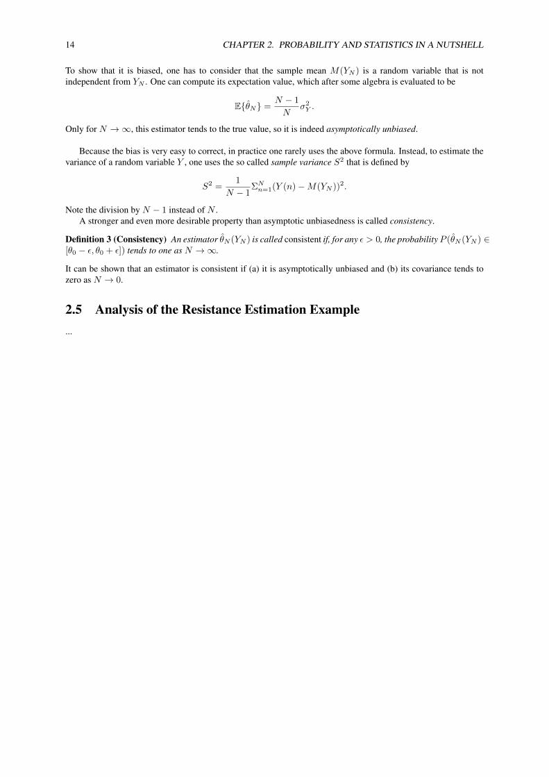
To show that it is biased, one has to consider that the sample mean M(YN ) is a random variable that is notindependent from YN . One can compute its expectation value, which after some algebra is evaluated to be
E{θN} =N − 1
Nσ2Y .
Only for N →∞, this estimator tends to the true value, so it is indeed asymptotically unbiased.
Because the bias is very easy to correct, in practice one rarely uses the above formula. Instead, to estimate thevariance of a random variable Y , one uses the so called sample variance S2 that is defined by
S2 =1
N − 1ΣNn=1(Y (n)−M(YN ))2.
Note the division by N − 1 instead of N .A stronger and even more desirable property than asymptotic unbiasedness is called consistency.
Definition 3 (Consistency) An estimator θN (YN ) is called consistent if, for any ε > 0, the probabilityP (θN (YN ) ∈[θ0 − ε, θ0 + ε]) tends to one as N →∞.
It can be shown that an estimator is consistent if (a) it is asymptotically unbiased and (b) its covariance tends tozero as N → 0.
2.5 Analysis of the Resistance Estimation Example...

ii
“msi” — 2014/11/26 — 15:16 — page 15 — #15 ii
ii
ii
Chapter 3
Linear Least Squares Estimation
Linear least squares (LLS or just LS) is a technique that helps us to find a model that is linear in some unknown pa-rameters θ ∈ Rd . For this aim, we regard a sequence of measurements y(1), . . . , y(N) ∈ R that shall be explained– they are also called the dependent variables – and another sequence of regression vectors φ(1), . . . , φ(N) ∈ Rd,which are regarded as the inputs of the model and are also called the independent or explanatory variables. Pre-diction errors are modelled by additive measurement noise ε(1), . . . , ε(N) with zero mean such that the overallmodel is given by
y(k) = φ(k)>θ + ε(k), for k = 1, . . . , N.
Let us in this section regard only scalar measurements y(k), though LLS can be generalized easily to the case ofseveral dependent variables. The task of LLS is to find an estimate θLS for the true but unknown parameter vectorθ0. Often the ultimate aim is to be able to predict a y for any given new values of the regression vector φ by themodel y = φ>θLS.
3.1 Least Squares Problem FormulationIdea of linear least squares is to find the θ that minimizes the sum of the squares of the prediction errors y(k) −φ(k)>θ, i.e. the least squares cost function
N∑k=1
(y(k)− φ(k)>θ
)2.
Stacking all values y(k) into one long vector yN ∈ RN and all regression vectors as rows into one matrix ΦN ∈RN×d, i.e.,
yN =
y(1)...
y(N)
and ΦN =
φ(1)>
...φ(N)>
we can write the least squares cost function1 as
f(θ) = ‖yN − ΦNθ‖22.
The least squares estimate θLS is the value of θ that minimizes this function. Thus, we are faced with an uncon-strained optimization problem that can be written as
minθ∈Rd
f(θ).
In estimation, we are mainly interested in the input arguments of f that achieve the minimal value, which we callthe minimizers. The set of minimizers S∗ is denoted by
S∗ = arg minθ∈Rd
f(θ).
1We recall that for any vector x ∈ Rn, we define the Euclidean norm as ‖x‖2 =(∑n
i=1 x2i
)1/2= (x>x)1/2.
15
ii
“msi” — 2014/11/26 — 15:16 — page 16 — #16 ii
ii
ii
16 CHAPTER 3. LINEAR LEAST SQUARES ESTIMATION
Note that there can be several minimizers. If the minimizer is unique, we have only one value in the set, that wedenote θ∗, and we can slightly sloppily identify θ∗ with {θ∗}. The least squares estimator θLS is given by thisunique minimizer, such that we will often write write
θLS = arg minθ∈Rd
f(θ).
But in order to compute the minimizer (or the set of minimizers), we need to solve an optimization problem. Letus therefore recall a few concepts from optimization, and then give an explicit solution formula for θLS.
3.2 A Micro-Review of Unconstrained OptimizationLet us in this section use, as customary in optimization textbooks, the variable x ∈ Rn instead of θ ∈ Rdas the unknown decision variable in the optimization problem. Throughout the course, we often want to solveunconstrained optimization problems of the form
minx∈D
f(x), (3.1)
where we regard objective functions f : D → R that are defined on some open domain D ⊂ Rn. We are onlyinterested in minimizers that lie inside of D. We might have D = Rn, but often this is not the case, e.g. as in thefollowing example:
minx∈(0,∞)
1
x+ x. (3.2)
Let us state a few simple and well-known results from unconstrained optimization that are often used in this course.
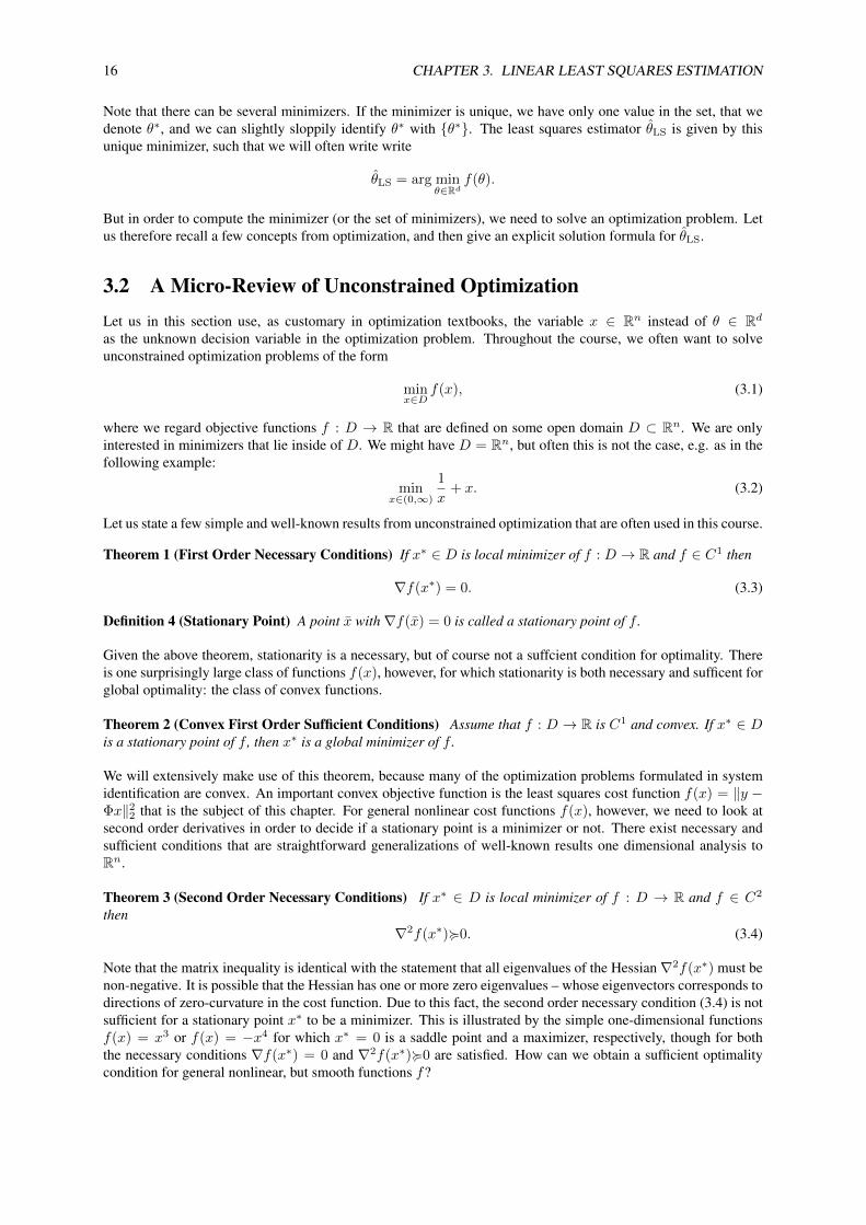
Theorem 1 (First Order Necessary Conditions) If x∗ ∈ D is local minimizer of f : D → R and f ∈ C1 then
∇f(x∗) = 0. (3.3)
Definition 4 (Stationary Point) A point x with∇f(x) = 0 is called a stationary point of f .
Given the above theorem, stationarity is a necessary, but of course not a suffcient condition for optimality. Thereis one surprisingly large class of functions f(x), however, for which stationarity is both necessary and sufficent forglobal optimality: the class of convex functions.
Theorem 2 (Convex First Order Sufficient Conditions) Assume that f : D → R is C1 and convex. If x∗ ∈ Dis a stationary point of f , then x∗ is a global minimizer of f .
We will extensively make use of this theorem, because many of the optimization problems formulated in systemidentification are convex. An important convex objective function is the least squares cost function f(x) = ‖y −Φx‖22 that is the subject of this chapter. For general nonlinear cost functions f(x), however, we need to look atsecond order derivatives in order to decide if a stationary point is a minimizer or not. There exist necessary andsufficient conditions that are straightforward generalizations of well-known results one dimensional analysis toRn.
Theorem 3 (Second Order Necessary Conditions) If x∗ ∈ D is local minimizer of f : D → R and f ∈ C2
then∇2f(x∗)<0. (3.4)
Note that the matrix inequality is identical with the statement that all eigenvalues of the Hessian∇2f(x∗) must benon-negative. It is possible that the Hessian has one or more zero eigenvalues – whose eigenvectors corresponds todirections of zero-curvature in the cost function. Due to this fact, the second order necessary condition (3.4) is notsufficient for a stationary point x∗ to be a minimizer. This is illustrated by the simple one-dimensional functionsf(x) = x3 or f(x) = −x4 for which x∗ = 0 is a saddle point and a maximizer, respectively, though for boththe necessary conditions ∇f(x∗) = 0 and ∇2f(x∗)<0 are satisfied. How can we obtain a sufficient optimalitycondition for general nonlinear, but smooth functions f?
ii
“msi” — 2014/11/26 — 15:16 — page 17 — #17 ii
ii
ii
3.3. SOLUTION OF THE LINEAR LEAST SQUARES PROBLEM 17
Theorem 4 (Second Order Sufficient Conditions and Stability under Perturbations) Assume that f : D →R is C2. If x∗ ∈ D is a stationary point and
∇2f(x∗)�0. (3.5)
then x∗ is a strict local minimizer of f . In addition, this minimizer is locally unique and is stable against smallperturbations of f , i.e.there exists a constant C such that for sufficiently small p ∈ Rn holds
‖x∗ − arg minx
(f(x)+p>x)‖ ≤ C‖p‖.
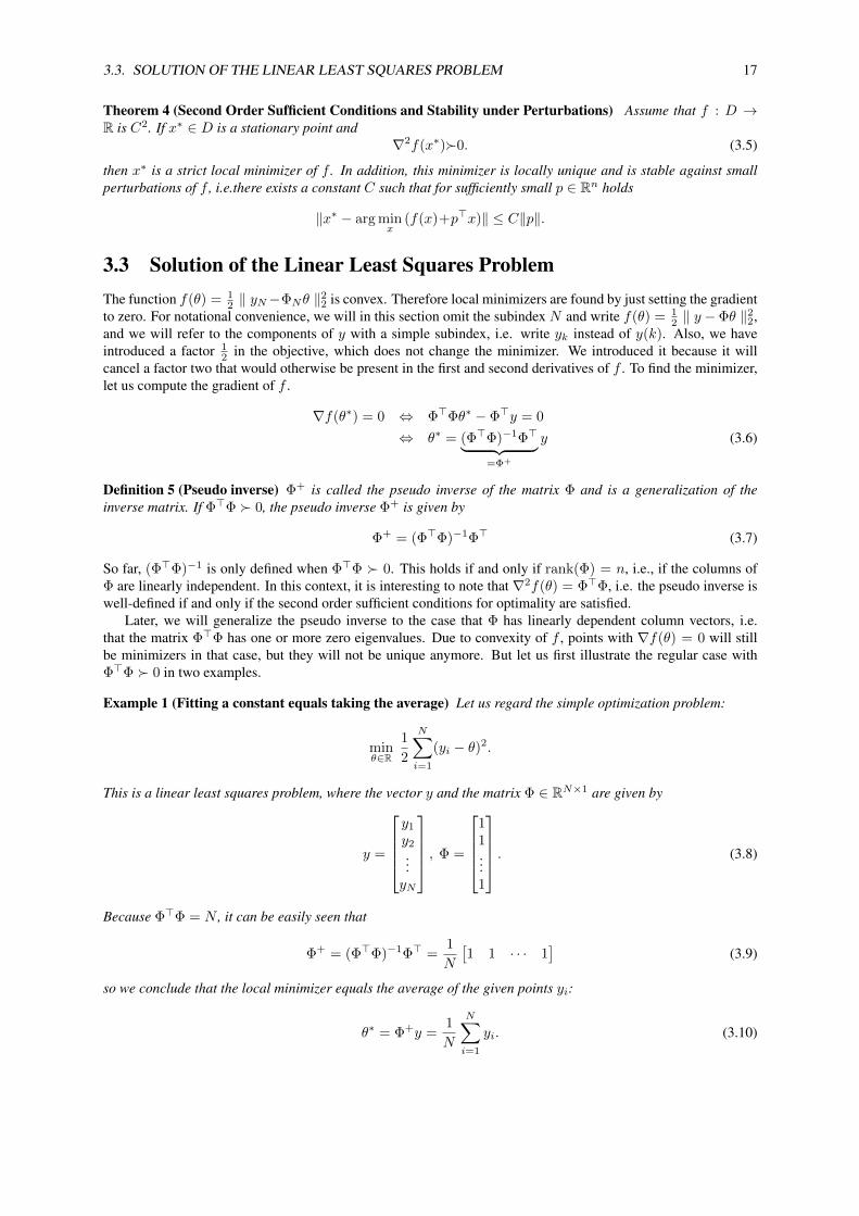
3.3 Solution of the Linear Least Squares ProblemThe function f(θ) = 1
2 ‖ yN−ΦNθ ‖22 is convex. Therefore local minimizers are found by just setting the gradientto zero. For notational convenience, we will in this section omit the subindex N and write f(θ) = 1
2 ‖ y −Φθ ‖22,and we will refer to the components of y with a simple subindex, i.e. write yk instead of y(k). Also, we haveintroduced a factor 1
2 in the objective, which does not change the minimizer. We introduced it because it willcancel a factor two that would otherwise be present in the first and second derivatives of f . To find the minimizer,let us compute the gradient of f .
∇f(θ∗) = 0 ⇔ Φ>Φθ∗ − Φ>y = 0
⇔ θ∗ = (Φ>Φ)−1Φ>︸ ︷︷ ︸=Φ+
y (3.6)
Definition 5 (Pseudo inverse) Φ+ is called the pseudo inverse of the matrix Φ and is a generalization of theinverse matrix. If Φ>Φ � 0, the pseudo inverse Φ+ is given by
Φ+ = (Φ>Φ)−1Φ> (3.7)
So far, (Φ>Φ)−1 is only defined when Φ>Φ � 0. This holds if and only if rank(Φ) = n, i.e., if the columns ofΦ are linearly independent. In this context, it is interesting to note that ∇2f(θ) = Φ>Φ, i.e. the pseudo inverse iswell-defined if and only if the second order sufficient conditions for optimality are satisfied.
Later, we will generalize the pseudo inverse to the case that Φ has linearly dependent column vectors, i.e.that the matrix Φ>Φ has one or more zero eigenvalues. Due to convexity of f , points with ∇f(θ) = 0 will stillbe minimizers in that case, but they will not be unique anymore. But let us first illustrate the regular case withΦ>Φ � 0 in two examples.
Example 1 (Fitting a constant equals taking the average) Let us regard the simple optimization problem:
minθ∈R
1
2
N∑i=1
(yi − θ)2.
This is a linear least squares problem, where the vector y and the matrix Φ ∈ RN×1 are given by
y =
y1
y2
...yN
, Φ =
11...1
. (3.8)
Because Φ>Φ = N , it can be easily seen that
Φ+ = (Φ>Φ)−1Φ> =1
N
[1 1 · · · 1
](3.9)
so we conclude that the local minimizer equals the average of the given points yi:
θ∗ = Φ+y =1
N
N∑i=1
yi. (3.10)
ii
“msi” — 2014/11/26 — 15:16 — page 18 — #18 ii
ii
ii
18 CHAPTER 3. LINEAR LEAST SQUARES ESTIMATION
ti
ηi
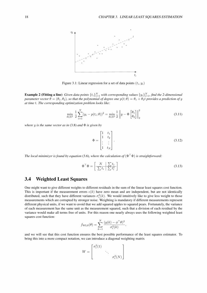
Figure 3.1: Linear regression for a set of data points (ti, yi)
Example 2 (Fitting a line) Given data points {ti}Ni=1 with corresponding values {yi}Ni=1, find the 2-dimensionalparameter vector θ = (θ1, θ2), so that the polynomial of degree one p(t; θ) = θ1 + θ2t provides a prediction of yat time t. The corresponding optimization problem looks like:
minθ∈R2
1
2
N∑i=1
(yi − p(ti; θ))2 = minθ∈R2
1
2
∥∥∥∥y − Φ
[θ1
θ2
]∥∥∥∥2
2
(3.11)
where y is the same vector as in (3.8) and Φ is given by
Φ =
1 t11 t2...
...1 tN
. (3.12)
The local minimizer is found by equation (3.6), where the calculation of (Φ>Φ) is straightforward:
Φ>Φ =
[N
∑ti∑
ti∑t2i
](3.13)
3.4 Weighted Least SquaresOne might want to give different weights to different residuals in the sum of the linear least squares cost function.This is important if the measurement errors ε(k) have zero mean and are independent, but are not identicallydistributed, such that they have different variances σ2
ε (k). We would intuitively like to give less weight to thosemeasurements which are corrupted by stronger noise. Weighting is mandatory if different measurements representdifferent physical units, if we want to avoid that we add squared apples to squared pears. Fortunately, the varianceof each measurement has the same unit as the measurement squared, such that a division of each residual by thevariance would make all terms free of units. For this reason one nearly always uses the following weighted leastsquares cost function:
fWLS(θ) =
N∑k=1
(y(k)− φ>θ)2
σ2ε (k)
,
and we will see that this cost function ensures the best possible performance of the least squares estimator. Tobring this into a more compact notation, we can introduce a diagonal weighting matrix
W =
σ2ε (1)
. . .σ2ε (N)

ii
“msi” — 2014/11/26 — 15:16 — page 19 — #19 ii
ii
ii
3.5. ILL-POSED LEAST SQUARES AND THE MOORE PENROSE PSEUDO INVERSE 19
and then write2
fWLS(θ) = ‖y − Φθ‖2W .Even more general, one might use any symmetric positive definite matrix W ∈ RN×N as weighting matrix. Theoptimal solution is given by
θWLS = arg min fWLS(θ) = (Φ>WΦ)−1Φ>Wy.
There is an alternative way to represent the solution, using the matrix Φ = W12 Φ and its pseudo inverse. To
derive this alternative way, let us first state the fact that there exists a unique symmetric square root W12 for any
symmetric positive definite matrix W . For example, for a diagonal weighting matrix as above, the square root isgiven by
W12 =
σε(1). . .
σε(N)
.With this square root matrix, we have the trivial identity ‖x‖2W = ‖W 1
2 ‖22 for any vector x ∈ RN and can thereforewrite
fWLS(θ) = ‖W 12 y︸ ︷︷ ︸
=:y
−W 12 Φ︸ ︷︷ ︸
=:Φ
θ‖2W .
Thus, the weighted least squares problem is nothing else than an unweighted least squares problem with rescaledmeasurements y = W
12 y and rescaled regressor matrix Φ = W
12 Φ, and the solution can be computed using the
pseudo inverse of Φ and is simply given byθWLS = Φ+y.
This way of computing the estimate is numerically more stable so it is in general preferable. An important obser-vation is that the resulting solution vector θWLS does not depend on the total scaling of the entries of the weightingmatrix, i.e. for any positive real number α, the weighting matrices W and αW deliver identical results θWLS.Only for this reason it is meaningful to use unweighted least squares – they deliver the optimal result in the casethat the measurement errors are assumed to be independent and identically distributed. But generally speaking, allleast squares problems are in fact weighted least squares problems, because one always has to make a choice ofhow to scale the measurement errors. If one uses unweighted least squares, one implicitly chooses the unit matrixas weighting matrix, which makes sense for i.i.d. measurement errors, but otherwise not. For ease of notation, wewill in the following nevertheless continue discussing the unweighted LS formulation, keeping in mind that anyweighted least squares problem can be brought into this form by the above rescaling procedure.
3.5 Ill-Posed Least Squares and the Moore Penrose Pseudo InverseIn some cases, the matrix Φ>Φ is not invertible, i.e. it contains at least one zero eigenvalue. In this case theestimation problem is called ill-posed, because the solution is not unique. But there is still the possibility to obtaina solution of the least squares problem that might give a reasonable result. For this we have to use a special type ofpseudo inverse. Let us recall that definition (3.7) of the pseudo inverse does only hold if Φ>Φ is invertible. Thisimplies that the set of optimal solutions S∗ has only one optimal point θ∗, given by S∗ = {θ∗} = (Φ>Φ)−1Φy. IfΦ>Φ is not invertible, the set of solutions S∗ is given by
S∗ = {θ | ∇f(θ) = 0} = {θ|Φ>Φθ − Φ>y = 0} (3.14)
In order to pick a unique point out of this set, we might choose to search for the “minimum norm solution”, i.e.the vector θ∗ with minimum norm satisfying θ∗ ∈ S∗.
minθ∈Rn
1
2‖θ‖22 subject to θ ∈ S∗ (3.15)
We will show below that this minimal norm solution is given by the so called “Moore Penrose Pseudo Inverse”.
2Recall that for any positive definite matrix W the weighted Euclidean norm ‖x‖W is defined as ‖x‖W =√x>Wx.
ii
“msi” — 2014/11/26 — 15:16 — page 20 — #20 ii
ii
ii
20 CHAPTER 3. LINEAR LEAST SQUARES ESTIMATION
x1
x2
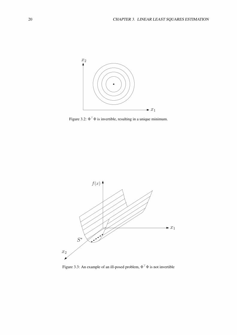
Figure 3.2: Φ>Φ is invertible, resulting in a unique minimum.
x1
x2
S∗
f(x)
Figure 3.3: An example of an ill-posed problem, Φ>Φ is not invertible
ii
“msi” — 2014/11/26 — 15:16 — page 21 — #21 ii
ii
ii
3.5. ILL-POSED LEAST SQUARES AND THE MOORE PENROSE PSEUDO INVERSE 21
Definition 6 (Moore Penrose Pseudo Inverse) Assume Φ ∈ Rm×n and that the singular value decomposition(SVD) of Φ is given by Φ = USV >. Then, the Moore Penrose Pseudo Inverse Φ+ is given by:
Φ+ = V S+U>, (3.16)
where for
S =
σ1
σ2
. . .σr
0. . .
00 . . . 0 . . . 0
holds S+ =
σ−11 0
σ−12
. . ....
σ−1r 0
0...
. . .0 0
(3.17)
If Φ>Φ is invertible, then Φ+ = (Φ>Φ)−1Φ> what easily can be shown:
(Φ>Φ)−1Φ> = (V S>U>USV >)−1V S>U>
= V (S>S)−1V >V S>U>
= V (S>S)−1S>U>
= V
σ2
1
σ22
. . .σ2r
−1
σ1
σ2 0. . .
σr
U>= V S+U>
3.5.1 Regularization for Least Squares
The minimum norm solution can be approximated by a “regularized problem”
minθ
1
2‖y − Φθ‖22 +
α
2‖θ‖22, (3.18)
with small α > 0, to get a unique solution
∇f(θ) = Φ>Φθ − Φ>y + αθ (3.19)= (Φ>Φ + αI)θ − Φ>y, (3.20)
thus θ∗ = (Φ>Φ + αI)−1Φ>y (3.21)(3.22)
Lemma 1 limα→0(Φ>Φ + αI)−1Φ> = Φ+, with Φ+ the Moore Penrose Pseudo Inverse.
Proof: Taking the SVD of Φ = USV >, (Φ>Φ + αI)−1Φ> can be written in the form:
(Φ>Φ + αI)−1Φ> = (V S>U>USV > + α I︸︷︷︸V V >
)−1 Φ>︸︷︷︸US>V >
= V (S>S + αI)−1V >V S>U>
= V (S>S + αI)−1S>U>
ii
“msi” — 2014/11/26 — 15:16 — page 22 — #22 ii
ii
ii
22 CHAPTER 3. LINEAR LEAST SQUARES ESTIMATION
Rewriting the right hand side of the equation explicitly:
= V
σ21 + α
. . .σ2r + α
α. . .
α
−1
σ1 0. . .
σr...
0. . .
0 0
U>
Calculating the matrix product simplifies the equation:
= V
σ1
σ21+α
0
. . .
σrσ2r+α
...0α
. . .0α 0
UT
It can be easily seen that for α→ 0 each diagonal element has the solution:
limα→0
σiσ2i + α
=
{1σi
if σi 6= 0
0 if σi = 0(3.23)
With the above lemma, we have shown that the Moore Penrose Pseudo Inverse Φ+ solves the problem (3.18) forinfinitely small α > 0. Thus it selects θ∗ ∈ S∗ with minimal norm.
3.6 Statistical Analysis of the Weighted Least Squares EstimatorIn the following, we analyse the weighted least squares estimator, and we make the following assumptions:
• the N measurements y(k) are generated by a model y(k) = φ(k)>θ0 + ε(k) with θ0 the true but unknownparameter value
• the N regression vectors φ(k) are deterministic and not corrupted by noise (attention: this assumption isoften violated in practice)
• the N noise terms ε(k) have zero mean. Often, we can also assume that they are independent from eachother, or even that they are i.i.d., and this will have consequences on the optimal choice of weighting matrix,as we will see. We abbreviate εN = [ε(1), . . . , ε(N)]>.
• the weighted least squares estimator is computed as θWLS = (Φ>NWΦN )−1Φ>NWyN .
We are most interested in the following questions: is the estimator biased or unbiased? What is its performance,i.e. what covariance matrix does the estimate have?
3.6.1 The expectation of the least squares estimator
Let us compute the expectation of θWLS.
E{θWLS} = E{
(Φ>NWΦN )−1Φ>NWyN}
(3.24)
= (Φ>NWΦN )−1Φ>NW E {yN} (3.25)
= (Φ>NWΦN )−1Φ>NW E {ΦNθ0 + εN } (3.26)
= (Φ>NWΦN )−1(Φ>NWΦN ) θ0 + (Φ>NWΦN )−1Φ>NW E {εN} (3.27)= θ0 + 0 (3.28)
Thus, the weighted least squares estimator has the true parameter value θ0 as expectation value, i.e. it is an unbiasedestimator. This fact is true independent of the choice of weighting matrix W .
ii
“msi” — 2014/11/26 — 15:16 — page 23 — #23 ii
ii
ii
3.7. MEASURING THE GOODNESS OF FIT USING R-SQUARED 23
3.6.2 The covariance of the least squares estimator
In order to assess the performance of an unbiased estimator, one can look at the covariance matrix of θWLS.The smaller this covariance matrix in the matrix sense, the better is the estimator. Let us therefore compute thecovariance matrix of θWLS. Using the identity θWLS − θ0 = (Φ>NWΦN )−1Φ>NWεN , it is given by
Cov(θWLS) = E{(θWLS − θ0)(θWLS − θ0)>} (3.29)
= (Φ>NWΦN )−1Φ>NW E{εN ε>N
}WΦN (Φ>NWΦN )−1 (3.30)
= (Φ>NWΦN )−1Φ>NW ΣεN WΦN (Φ>NWΦN )−1. (3.31)
Here, we have used the shorthand ΣεN = Cov(ε)N). For different choices of W , the covariance Cov(θWLS) willbe different. However, there is one specific choice that makes the above formula very easy: if we happen to knowΣεN and would choose W := Σ−1
εN , we would obtain
Cov(θWLS) = (Φ>NWΦN )−1Φ>NW W−1 WΦN (Φ>NWΦN )−1 (3.32)
= (Φ>NWΦN )−1(Φ>NWΦN )(Φ>NWΦN )−1 (3.33)
= (Φ>NWΦN )−1 (3.34)
= (Φ>NΣ−1εN ΦN )−1. (3.35)
Interestingly, it turns out that this choice of weighting matrix is the optimal choice, i.e. for all other weightingmatrices W one has
Cov(θWLS)<(Φ>NΣ−1εN ΦN )−1.
Even more, one can show that in case of Gaussian noise with zero mean and covariance ΣεN , the weighted linearleast squares estimator with optimal weights W = Σ−1
εN achieves the lower bound on the covariance matrix thatany unbiased estimator can achieve (the so called Cramer-Rao lower bound).
3.7 Measuring the Goodness of Fit using R-SquaredOne ... Coefficient of Determination - R2 ...
3.8 Estimating the Covariance with a Single ExperimentSo far, we have analysed the theoretical properties of the LS estimator, and we know that for independent identi-cally distributed measurement errors, the unweighted least squares estimater gives us the optimal estimator. If thevariance of the noise is σ2
ε , the least squares estimator θLS = Φ+NyN is a random variable with the true parameter
value θ0 as mean and the following covariance matrix:
Σθ := Cov(θLS) = σ2ε (Φ>NΦN )−1.
In addition, if the number of measurementN in one experiment is large, by a law of large numbers, the distributionof θLS follows approximately a normal distribution, even if the measurement errors were not normally distributed.Thus, if one repeats the same experiment with the same N regression vectors many times, the estimates θLS
would follow a normal distribution characterized by these two parameters, i.e. θLS ∼ N (θ0,Σθ). In a realisticapplication, however, the situation is quite different than in this analysis:
• First, we do of course not know the true value θ0
• Second, we do not repeat our experiment many times, but just do one single experiment.
• Third, we typically do not know the variance of the measurement noise σ2ε .
Nevertheless, and surprisingly, if one makes the assumption that the noise is independent identically distributed,one is able to make a very good guess of the covariance matrix of the estimator, which we will describe here.The main reason is that we know the deterministic matrix ΦN exactly. The covariance is basically given by thematrix (Φ>NΦ)−1, which only needs to be scaled by a factor, the unknown σ2
ε . Thus, we only need to find an
ii
“msi” — 2014/11/26 — 15:16 — page 24 — #24 ii
ii
ii
24 CHAPTER 3. LINEAR LEAST SQUARES ESTIMATION
estimate for the noise variance. Fortunately, we have N measurements y(k) as well as the corresponding modelpredictions φ(k)>θLS for k = 1, . . . , N , so their average difference can be used to estimate the measurement noise.Because the predictions are based on fitting the d-dimensional vector θLS to the same measurements y(k) that wewant to use to estimate the measurement errors, we should not just take the average of the squared deviations(y(k) − φ(k)>θ)2 – this would be a biased (though asymptotically unbiased) estimator. It can be shown that anunbiased estimate for σ2
ε is obtained by
σ2ε :=
1
(N − d)
N∑k=1
(y(k)− φ(k)>θLS)2 =‖yN − ΦN θLS‖22
(N − d)
Thus, our final formula for a good estimate Σθ of the true but unknown covariance Cov(θLS) is
Σθ := σ2ε (Φ>NΦN )−1 =
‖yN − ΦN θLS‖22(N − d)
(Φ>NΦN )−1.
What we have now are two quantities, an estimate θLS of the true parameter value θ0, as well as an estimate Σθ forthe covariance matrix of this estimate. This knowledge helps us to make a strong statement about how probable itis that our our estimate is close to the true parameter value. Under the assumption that our linear model structureis correct and thus our estimator is unbiased, and the (slightly optimistic) assumption that our covariance estimateΣθ is equal to the true covariance Σθ of the estimator θLS, we can compute the probability that an uncertaintyellipsoid around the estimated θLS contains the (unknown) true parameter value θ0.
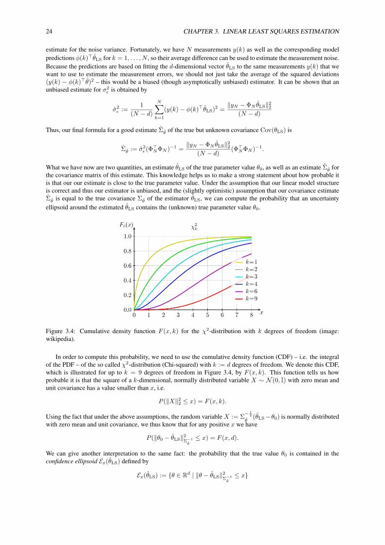
Figure 3.4: Cumulative density function F (x, k) for the χ2-distribution with k degrees of freedom (image:wikipedia).
In order to compute this probability, we need to use the cumulative density function (CDF) – i.e. the integralof the PDF – of the so called χ2-distribution (Chi-squared) with k := d degrees of freedom. We denote this CDF,which is illustrated for up to k = 9 degrees of freedom in Figure 3.4, by F (x, k). This function tells us howprobable it is that the square of a k-dimensional, normally distributed variable X ∼ N (0, I) with zero mean andunit covariance has a value smaller than x, i.e.
P (‖X‖22 ≤ x) = F (x, k).
Using the fact that under the above assumptions, the random variableX := Σ− 1
2
θ(θLS−θ0) is normally distributed
with zero mean and unit covariance, we thus know that for any positive x we have
P (‖θ0 − θLS‖2Σ−1
θ
≤ x) = F (x, d).
We can give another interpretation to the same fact: the probability that the true value θ0 is contained in theconfidence ellipsoid Ex(θLS) defined by
Ex(θLS) := {θ ∈ Rd | ‖θ − θLS‖2Σ−1
θ
≤ x}
ii
“msi” — 2014/11/26 — 15:16 — page 25 — #25 ii
ii
ii
3.8. ESTIMATING THE COVARIANCE WITH A SINGLE EXPERIMENT 25
is given byP(θ0 ∈ Ex(θLS)
)= F (x, d).
Note that in this expression, it is the ellipsoid which is random, not the true, but unknown, value θ0. We call theconfidence ellipsoid for x = 1, i.e. the set
E1(θLS) := {θ ∈ Rd | ‖θ − θLS‖2Σ−1
θ
≤ 1}
the one-sigma confidence ellipsoid. The probability that the true value is contained in it decreases with increasingdimension d = k of the parameter space and can be found in Figure 3.4 at x = 1.
Note that the variance for one single component of the parameter vector can be found as a diagonal entry inthe covariance matrix, and that the probability that the true value of this single component is inside the one sigmainterval around the estimated value is always 68.3%, independent of the parameter dimension d. This is due to thefact that each single component of θ follows a one dimensional normal distribution.
For mathematical correctness, we have to note that we had to assume that the covariance matrix Σθ is exactlyknown in order to make use of the χ2-distribution. On the other hand, in practice, we can only use its estimateΣθ in the definition of the confidence ellipsoid. A refined analysis, which is beyond our ambitions, would need to
take into account that also Σθ is a random variable, which implies that X := Σ− 1
2
θ(θLS−θ0) follows a distribution
which is similar to, but not equal to a standard normal distribution. For the practice of least squares estimation,however, the above characterization of confidence ellipsoids with the χ2-distribution is accurate enough and canhelp us to assess the quality of an estimation result after a single experiment.

ii
“msi” — 2014/11/26 — 15:16 — page 26 — #26 ii
ii
ii
26 CHAPTER 3. LINEAR LEAST SQUARES ESTIMATION
ii
“msi” — 2014/11/26 — 15:16 — page 27 — #27 ii
ii
ii
Chapter 4
Maximum Likelihood and BayesianEstimation
...
4.1 Maximum Likelihood Estimation
Definition 7 (Likelihood) The likelihood function L(θ) is a function of θ for given measurements y that describeshow likely the measurements would have been if the parameter would have the value θ. It is defined as L(θ) =p(y|θ), using the PDF of y for given θ.
Definition 8 (Maximum-Likelihood Estimate) The maximum-likelihood estimate of the unknown parameter θis the parameter value that maximizes the likelihood function L(θ) = p(y|θ).
Assume yi = Mi(θ) + εi with θ the “true” parameter, and εi Gaussian noise with expectation value E(εi) = 0,E(εi εi) = σ2
i and εi, εj independent for i 6= j . Then holds
p(y|θ) =
m∏i=1
p(yi | θ) (4.1)
= C
m∏i=1
exp
(−(yi −Mi(θ))2
2σ2i
)(4.2)
with C =∏mi=1
1√2πσ2
i
. Taking the logarithm of both sides gives
log p(y|θ) = log(C) +
m∑i=1
− (yi −Mi(θ))2
2σ2i
(4.3)
with a constant C. Due to monotonicity of the logarithm holds that the argument maximizing p(y|θ) is given by
arg maxθ∈Rn
p(y|θ) = arg minθ∈Rn
− log(p(y|θ)) (4.4)
= arg minθ∈Rn
m∑i=1
(yi −Mi(θ))2
2σ2i
(4.5)
= arg minθ∈Rn
1
2‖S−1(y −M(θ))‖22 (4.6)
Thus, the least squares problem has a statistical interpretation. Note that due to the fact that we might have differentstandard deviations σi for different measurements yi we need to scale both measurements and model functions in
27

ii
“msi” — 2014/11/26 — 15:16 — page 28 — #28 ii
ii
ii
28 CHAPTER 4. MAXIMUM LIKELIHOOD AND BAYESIAN ESTIMATION
order to obtain an objective in the usual least squares form ‖y − M(θ)‖22, as
minθ
1
2
n∑i=1
(yi −Mi(θ)
σi
)2
= minθ
1
2‖S−1(y −M(θ))‖22 (4.7)
= minθ
1
2‖S−1y − S−1M(θ)‖22 (4.8)
with S =
σ1
. . .σm
.Statistical Interpretation of Regularization terms: Note that a regularization term like α‖θ − θ‖22 that isadded to the objective can be interpreted as a “pseudo measurement” θ of the parameter value θ, which includesa statistical assumption: the smaller α, the larger we implicitly assume the standard deviation of this pseudo-measurement. As the data of a regularization term are usually given before the actual measurements, regularizationis also often interpreted as “a priori knowledge”. Note that not only the Euclidean norm with one scalar weightingα can be chosen, but many other forms of regularization are possible, e.g. terms of the form ‖A(θ − θ)‖22 withsome matrix A.
4.1.1 L1-EstimationInstead of using ‖.‖22, i.e. the L2-norm in the fitting problem, we might alternatively use ‖.‖1, i.e., the L1-norm.This gives rise to the so called L1-estimation problem:
minθ‖y −M(θ)‖1 = min
θ
m∑i=1
|yi −Mi(θ)| (4.9)
Like the L2-estimation problem, also the L1-estimation problem can be interpreted statistically as a maximum-likelihood estimate. However, in the L1-case, the measurement errors are assumed to follow a Laplace distributioninstead of a Gaussian.
An interesting observation is that the optimal L1-fit of a constant θ to a sample of different scalar valuesy1, . . . , ym just gives the median of this sample, i.e.
arg minθ∈R
m∑i=1
|yi − θ| = median of {y1, . . . , ym}. (4.10)
Remember that the same problem with the L2-norm gave the average of yi. Generally speaking, the median is lesssensitive to outliers than the average, and a detailed analysis shows that the solution to general L1-estimation prob-lems is also less sensitive to a few outliers. Therefore, L1-estimation is sometimes also called “robust” parameterestimation.
4.2 Bayesian Estimation and the Maximum A Posteriori Estimate...
4.3 Recursive Linear Least Squares...
ii
“msi” — 2014/11/26 — 15:16 — page 29 — #29 ii
ii
ii
Chapter 5
Dynamic Systems in a Nutshell
In this lecture, our major aim is to model and identify dynamic systems, i.e. processes that are evolving with time.These systems can be characterized by states x and parameters p that allow us to predict the future behavior ofthe system. If the state and the parameters are not known, we first need to estimate them based on the availablemeasurement information. The estimation process is very often optimization-based, and thus, derivatives play acrucial role in this chapter. Often, a dynamic system can be controlled by a suitable choice of inputs that we denoteas controls u in this script, and the ultimate purpose of modelling and system identification is to be able to designand test control strategies.
As an example of a dynamic system, we might think of an electric train where the state x consists of the currentposition and velocity, and where the control u is the engine power that the train driver can choose at each moment.We might regard the motion of the train on a time interval [tinit, tfin], and the ultimate aim of controller designcould be to minimize the consumption of electrical energy while arriving in time. Before we can decide on thecontrol strategy, we need to know the current state of the train. Even more important, we should know importantmodel parameters such as the mass of the train or how the motor efficiency changes with speed.
To determine the unknown system parameters, we typically perform experiments and record measurementdata. In optimization-based state and parameter estimation, the objective function is typically the misfit betweenthe actual measurements and the model predictions.
A typical property of a dynamic system is that knowledge of an initial state xinit and a control input trajectoryu(t) for all t ∈ [tinit, tfin] allows one to determine the whole state trajectory x(t) for t ∈ [tinit, tfin]. As the motionof a train can very well be modelled by Newton’s laws of motion, the usual description of this dynamic system isdeterministic and in continuous time and with continuous states.
But dynamic systems and their mathematical models can come in many variants, and it is useful to properlydefine the names given commonly to different dynamic system classes, which we do in the next section. After-wards, we will discuss two important classes, continuous time and discrete time systems, in more mathematicaldetail.
5.1 Dynamic System Classes
In this section, let us go, one by one, through the many dividing lines in the field of dynamic systems.
Continuous vs Discrete Time Systems
Any dynamic system evolves over time, but time can come in two variants: while the physical time is continu-ous and forms the natural setting for most technical and biological systems, other dynamic systems can best bemodelled in discrete time, such as digitally controlled sampled-data systems, or games.
We call a system a discrete time system whenever the time in which the system evolves only takes values on apredefined time grid, usually assumed to be integers. If we have an interval of real numbers, like for the physicaltime, we call it a continuous time system. In this lecture, we usually denote the continuous time by the variablet ∈ R and write for example x(t). In case of discrete time systems, we typically use the index variable k ∈ N, andwrite xk or x(k) for the state at time point k.
29
ii
“msi” — 2014/11/26 — 15:16 — page 30 — #30 ii
ii
ii
30 CHAPTER 5. DYNAMIC SYSTEMS IN A NUTSHELL
Continuous vs Discrete State Spaces
Another crucial element of a dynamic system is its state x, which often lives in a continuous state space, like theposition of the train, but can also be discrete, like the position of the figures on a chess game. We define the statespace X to be the set of all values that the state vector x may take. If X is a subset of a real vector space such asRnx or another differentiable manifold, we speak of a continuous state space. If X is a finite or a countable set, wespeak of a discrete state space. If the state of a system is described by a combination of discrete and continuousvariables we speak of a hybrid state space.
Finite vs Infinite Dimensional State Spaces
The class of continuous state spaces can be further subdivided into the finite dimensional ones, whose state canbe characterized by a finite set of real numbers, and the infinite dimensional ones, which have a state that lives infunction spaces. The evolution of finite dimensional systems in continuous time is usually described by ordinarydifferential equations (ODE) or their generalizations, such as differential algebraic equations (DAE).
Infinite dimensional systems are sometimes also called distributed parameter systems, and in the continuoustime case, their behaviour is typically described by partial differential equations (PDE). An example for a con-trolled infinite dimensional system is the evolution of the airflow and temperature distribution in a building that iscontrolled by an air-conditioning system. Systems with delay are another class of systems with infinite dimensionalstate space.
Continuous vs Discrete Control Sets
We denote by U the set in which the controls u live, and exactly as for the states, we can divide the possible controlsets into continuous control sets and discrete control sets. A mixture of both is a hybrid control set. An examplefor a discrete control set is the set of gear choices for a car, or any switch that we can can choose to be either on oroff, but nothing in between.
Time-Variant vs Time-Invariant Systems
A system whose dynamics depend on time is called a time-variant system, while a dynamic system is called time-invariant if its evolution does not depend on the time and date when it is happening. As the laws of physics aretime-invariant, most technical systems belong to the latter class, but for example the temperature evolution of ahouse with hot days and cold nights might best be described by a time-variant system model. While the classof time-variant systems trivially comprises all time-invariant systems, it is an important observation that also theother direction holds: each time-variant system can be modelled by a nonlinear time-invariant system if the statespace is augmented by an extra state that takes account of the advancement of time, and which we might call the“clock state”.
Linear vs Nonlinear Systems
If the state trajectory of a system depends linearly on the initial value and the control inputs, it is called a linearsystem. If the dependence is affine, one should ideally speak of an affine system, but often the term linear is usedhere as well. In all other cases, we speak of a nonlinear system.
A particularly important class of linear systems are linear time invariant (LTI) systems. An LTI system can becompletely characterized in at least three equivalent ways: first, by two matrices that are typically called A and B;second, by its step response function; and third, by its frequency response function. A large part of the research inthe control community is devoted to the study of LTI systems.
Controlled vs Uncontrolled Dynamic Systems
While we are in this lecture mostly interested in controlled dynamic systems, i.e. systems that have a control inputthat we can choose, it is good to remember that there exist many systems that cannot be influenced at all, but thatonly evolve according to their intrinsic laws of motion. These uncontrolled systems have an empty control set,U = ∅. If a dynamic system is both uncontrolled and time-invariant it is also called an autonomous system.
ii
“msi” — 2014/11/26 — 15:16 — page 31 — #31 ii
ii
ii
5.2. CONTINUOUS TIME SYSTEMS 31
Stable vs Unstable Dynamic Systems
A dynamic system whose state trajectory remains bounded for bounded initial values and controls is called a stablesystem, and an unstable system otherwise. For autonomous systems, stability of the system around a fixed pointcan be defined rigorously: for any arbitrarily small neighborhoodN around the fixed point there exists a region sothat all trajectories that start in this region remain in N . Asymptotic stability is stronger and additionally requiresthat all considered trajectories eventually converge to the fixed point. For autonomous LTI systems, stability canbe computationally characterized by the eigenvalues of the system matrix.
Deterministic vs Stochastic Systems
If the evolution of a system can be predicted when its initial state and the control inputs are known, it is called adeterministic system. When its evolution involves some random behaviour, we call it a stochastic system.
The movements of assets on the stockmarket are an example for a stochastic system, whereas the motion ofplanets in the solar system can usually be assumed to be deterministic. An interesting special case of deterministicsystems with continuous state space are chaotic systems. These systems are so sensitive to their initial values thateven knowing these to arbitrarily high, but finite, precisions does not allow one to predict the complete future of thesystem: only the near future can be predicted. The partial differential equations used in weather forecast modelshave this property, and one well-known chaotic system of ODE, the Lorenz attractor, was inspired by these.
Open-Loop vs Closed-Loop Controlled Systems
When choosing the inputs of a controlled dynamic system, one first way is decide in advance, before the processstarts, which control action we want to apply at which time instant. This is called open-loop control in the systemsand control community, and has the important property that the control u is a function of time only and does notdepend on the current system state.
A second way to choose the controls incorporates our most recent knowledge about the system state whichwe might observe with the help of measurements. This knowledge allows us to apply feedback to the system byadapting the control action according to the measurements. In the systems and control community, this is calledclosed-loop control, but also the more intuitive term feedback control is used. It has the important property thatthe control action does depend on the current state or the latest measurements.
5.2 Continuous Time SystemsMost systems of interest in science and engineering are described in form of deterministic differential equationswhich live in continuous time. On the other hand, all numerical simulation methods have to discretize the timeinterval of interest in some form or the other and thus effectively generate discrete time systems. We will thusbriefly sketch some relevant properties of continuous time systems in this section, and show how they can betransformed into discrete time systems. Later, we will mainly be concerned with discrete time systems, while weoccasionally come back to the continuous time case.
Ordinary Differential Equations
A controlled dynamic system in continuous time can in the simplest case be described by an ordinary differentialequation (ODE) on a time interval [tinit, tfin] by
x(t) = f(x(t), u(t), t), t ∈ [tinit, tfin] (5.1)
where t ∈ R is the time, u(t) ∈ Rnu are the controls, and x(t) ∈ Rnx is the state. The function f is a map fromstates, controls, and time to the rate of change of the state, i.e. f : Rnx × Rnu × [tinit, tfin] → Rnx . Due to theexplicit time dependence of the function f , this is a time-variant system.
We are first interested in the question if this differential equation has a solution if the initial value x(tinit) isfixed and also the controls u(t) are fixed for all t ∈ [tinit, tfin]. In this context, the dependence of f on the fixedcontrols u(t) is equivalent to a a further time-dependence of f , and we can redefine the ODE as x = f(x, t) withf(x, t) := f(x, u(t), t). Thus, let us first leave away the dependence of f on the controls, and just regard thetime-dependent uncontrolled ODE:
x(t) = f(x(t), t), t ∈ [tinit, tfin]. (5.2)
ii
“msi” — 2014/11/26 — 15:16 — page 32 — #32 ii
ii
ii
32 CHAPTER 5. DYNAMIC SYSTEMS IN A NUTSHELL
Initial Value Problems
An initial value problem (IVP) is given by (5.2) and the initial value constraint x(tinit) = xinit with some fixedparameter xinit. Existence of a solution to an IVP is guaranteed under continuity of f with respect to to x and taccording to a theorem from 1886 that is due to Giuseppe Peano. But existence alone is of limited interest as thesolutions might be non-unique.
Example 3 (Non-Unique ODE Solution) The scalar ODE with f(x) =√|x(t)| can stay for an undetermined
duration in the point x = 0 before leaving it at an arbitrary time t0. It then follows a trajectory x(t) = (t− t0)2/4that can be easily shown to satisfy the ODE (5.2). We note that the ODE function f is continuous, and thusexistence of the solution is guaranteed mathematically. However, at the origin, the derivative of f approachesinfinity. It turns out that this is the reason which causes the non-uniqueness of the solution.
As we are only interested in systems with well-defined and deterministic solutions, we would like to formulateonly ODE with unique solutions. Here helps the following theorem by Charles Emile Picard (1890) and ErnstLeonard Lindelof (1894).
Theorem 5 (Existence and Uniqueness of IVP) Regard the initial value problem (5.2) with x(tinit) = xinit, andassume that f : Rnx × [tinit, tfin] → Rnx is continuous with respect to x and t. Furthermore, assume that fis Lipschitz continuous with respect to x, i.e., that there exists a constant L such that for all x, y ∈ Rnx and allt ∈ [tinit, tfin]
‖f(x, t)− f(y, t)‖ ≤ L‖x− y‖. (5.3)
Then there exists a unique solution x : [tinit, tfin]→ Rnx of the IVP.
Lipschitz continuity of f with respect to x is not easy to check. It is much easier to verify if a function is differ-entiable. It is therefore a helpful fact that every function f that is differentiable with respect to x is also locallyLipschitz continuous, and one can prove the following corollary to the Theorem of Picard-Lindelof.
Corollary 1 (Local Existence and Uniqueness) Regard the same initial value problem as in Theorem 5, but in-stead of global Lipschitz continuity, assume that f is continuously differentiable with respect to x for all t ∈[tinit, tfin]. Then there exists a possibly shortened, but non-empty interval [tinit, t
′fin] with t′fin ∈ (tinit, tfin] on
which the IVP has a unique solution.
Note that for nonlinear continuous time systems – in contrast to discrete time systems – it is very easily possibleto obtain an “explosion”, i.e., a solution that tends to infinity for finite times, even with innocently looking andsmooth functions f .
Example 4 (Explosion of an ODE) Regard the scalar example f(x) = x2 with tinit = 0 and xinit = 1, and letus regard the interval [tinit, tfin] with tfin = 10. The IVP has the explicit solution x(t) = 1/(1 − t), which isonly defined on the half open interval [0, 1), because it tends to infinity for t → 1. Thus, we need to choose somet′fin < 1 in order to have a unique and finite solution to the IVP on the shortened interval [tinit, t
′fin]. The existence
of this local solution is guaranteed by the above corollary. Note that the explosion in finite time is due to the factthat the function f is not globally Lipschitz continuous, so Theorem 5 is not applicable.
Discontinuities with Respect to Time
It is important to note that the above theorem and corollary can be extended to the case that there are finitely manydiscontinuities of f with respect to t. In this case the ODE solution can only be defined on each of the continuoustime intervals separately, while the derivative of x is not defined at the time points at which the discontinuitiesof f occur, at least not in the strong sense. But the transition from one interval to the next can be determined bycontinuity of the state trajectory, i.e. we require that the end state of one continuous initial value problem is thestarting value of the next one.
The fact that unique solutions still exist in the case of discontinuities is important because many state andparameter estimation problems are based on discontinuous control trajectories u(t). Fortunately, this does notcause difficulties for existence and uniqueness of the IVPs.
ii
“msi” — 2014/11/26 — 15:16 — page 33 — #33 ii
ii
ii
5.2. CONTINUOUS TIME SYSTEMS 33
Linear Time Invariant (LTI) Systems
A special class of tremendous importance are the linear time invariant (LTI) systems. These are described by anODE of the form
x = Ax+Bu (5.4)
with fixed matrices A ∈ Rnx×nx and B ∈ Rnx×nu . LTI systems are one of the principal interests in the fieldof automatic control and a vast literature exists on LTI systems. Note that the function f(x, u) = Ax + Bu isLipschitz continuous with respect to x with Lipschitz constant L = ‖A‖, so that the global solution to any initialvalue problem with a piecewise continuous control input can be guaranteed.
For system identification, we usually need to add output equations y = Cx + Du to our model, where theoutputs y may be the only physically measurable quantities. In that context, it is important to remark that the statesare not even unique, because different state space realizations of the same input-output behavior exist.
Many important notions such as controllability or stabilizability, and observability or detectability, and con-cepts such as the impulse response or frequency response function can be defined in terms of the matrices A,B,Cand D alone. In particular, the transfer function G(s) of an LTI system is the Laplace transform of the impulseresponse can be shown to be given by
G(s) = C(sI −A)−1B +D.
The frequency response is given by the transfer function evaluated at values s = jω where j is the imaginary unit.
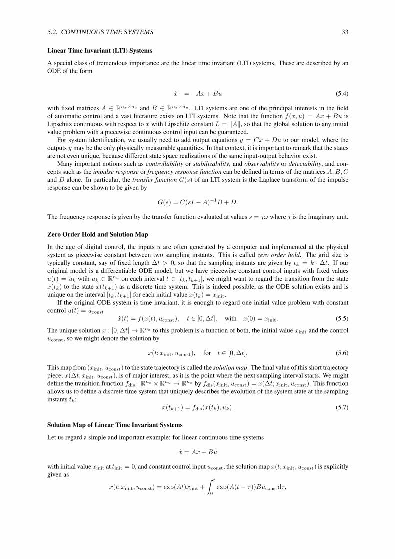
Zero Order Hold and Solution Map
In the age of digital control, the inputs u are often generated by a computer and implemented at the physicalsystem as piecewise constant between two sampling instants. This is called zero order hold. The grid size istypically constant, say of fixed length ∆t > 0, so that the sampling instants are given by tk = k · ∆t. If ouroriginal model is a differentiable ODE model, but we have piecewise constant control inputs with fixed valuesu(t) = uk wtih uk ∈ Rnu on each interval t ∈ [tk, tk+1], we might want to regard the transition from the statex(tk) to the state x(tk+1) as a discrete time system. This is indeed possible, as the ODE solution exists and isunique on the interval [tk, tk+1] for each initial value x(tk) = xinit.
If the original ODE system is time-invariant, it is enough to regard one initial value problem with constantcontrol u(t) = uconst
x(t) = f(x(t), uconst), t ∈ [0,∆t], with x(0) = xinit. (5.5)
The unique solution x : [0,∆t]→ Rnx to this problem is a function of both, the initial value xinit and the controluconst, so we might denote the solution by
x(t;xinit, uconst), for t ∈ [0,∆t]. (5.6)
This map from (xinit, uconst) to the state trajectory is called the solution map. The final value of this short trajectorypiece, x(∆t;xinit, uconst), is of major interest, as it is the point where the next sampling interval starts. We mightdefine the transition function fdis : Rnx ×Rnu → Rnx by fdis(xinit, uconst) = x(∆t;xinit, uconst). This functionallows us to define a discrete time system that uniquely describes the evolution of the system state at the samplinginstants tk:
x(tk+1) = fdis(x(tk), uk). (5.7)
Solution Map of Linear Time Invariant Systems
Let us regard a simple and important example: for linear continuous time systems
x = Ax+Bu
with initial value xinit at tinit = 0, and constant control input uconst, the solution map x(t;xinit, uconst) is explicitlygiven as
x(t;xinit, uconst) = exp(At)xinit +
∫ t
0
exp(A(t− τ))Buconstdτ,

ii
“msi” — 2014/11/26 — 15:16 — page 34 — #34 ii
ii
ii
34 CHAPTER 5. DYNAMIC SYSTEMS IN A NUTSHELL
where exp(A) is the matrix exponential. It is interesting to note that this map is well defined for all times t ∈ R,as linear systems cannot explode. The corresponding discrete time system with sampling time ∆t is again a lineartime invariant system, and is given by
fdis(xk, uk) = Adisxk +Bdisuk (5.8)
with
Adis = exp(A∆t) and Bdis =
∫ ∆t
0
exp(A(∆t− τ))Bdτ. (5.9)
One interesting observation is that the discrete time system matrix Adis resulting from the solution of an LTIsystem in continuous time is by construction an invertible matrix, with inverse A−1
dis = exp(−A∆t). For systemswith strongly decaying dynamics, however, the matrix Adis might have some very small eigenvalues and will thusbe nearly singular.
Sensitivities
In the context of estimation, derivatives of the dynamic system simulation are often needed. Following Theorem 5and Corollary 1 we know that the solution map to the IVP (5.5) exists on an interval [0,∆t] and is unique undermild conditions even for general nonlinear systems. But is it also differentiable with respect to the initial value andcontrol input?
In order to discuss the issue of derivatives, which in the dynamic system context are often called sensitivities,let us first ask what happens if we call the solution map with different inputs. For small perturbations of the values(xinit, uconst), we still have a unique solution x(t;xinit, uconst) on the whole interval t ∈ [0,∆t]. Let us restrictourselves to a neighborhood N of fixed values (xinit, uconst). For each fixed t ∈ [0,∆t], we can now regardthe well defined and unique solution map x(t; ·) : N → Rnx , (xinit, uconst) 7→ x(t;xinit, uconst). A naturalquestion to ask is if this map is differentiable. Fortunately, it is possible to show that if f is m-times continuouslydifferentiable with respect to both x and u, then the solution map x(t; ·), for each t ∈ [0,∆t], is also m-timescontinuously differentiable with respect to (xinit, uconst).
In the general nonlinear case, the solution map x(t;xinit, uconst) can only be generated by a numerical simu-lation routine. The computation of derivatives of this numerically generated map is a delicate issue. The reasonis that most numerical integration routines are adaptive, i.e., might choose to do different numbers of integrationsteps for different IVPs. This renders the numerical approximation of the map x(t;xinit, uconst) typically non-differentiable in the inputs xinit, uconst. Thus, multiple calls of a black-box integrator and application of finitedifferences might result in very wrong derivative approximations.
Numerical Integration Methods
A numerical simulation routine that approximates the solution map is often called an integrator. A simple but verycrude way to generate an approximation for x(t;xinit, uconst) for t ∈ [0,∆t] is to perform a linear extrapolationbased on the time derivative x = f(x, u) at the initial time point:
x(t;xinit, uconst) = xinit + tf(xinit, uconst), t ∈ [0,∆t]. (5.10)
This is called one Euler integration step. For very small ∆t, this approximation becomes very good. In fact,the error x(∆t;xinit, uconst) − x(∆t;xinit, uconst) is of second order in ∆t. This motivated Leonhard Euler toperform several steps of smaller size, and propose what is now called the Euler integration method. We subdividethe interval [0,∆t] into M subintervals each of length h = ∆t/M , and perform M such linear extrapolation stepsconsecutively, starting at x0 = xinit:
xj+1 = xj + hf(xj , uconst), j = 0, . . . ,M − 1. (5.11)
It can be proven that the Euler integration method is stable, i.e. that the propagation of local errors is bounded witha constant that is independent of the step size h. Therefore, the approximation becomes better and better when wedecrease the step size h: since the consistency error in each step is of order h2, and the total number of steps is oforder ∆t/h, the accumulated error in the final step is of order h∆t. As this is linear in the step size h, we say thatthe Euler method has the order one. Taking more steps is more accurate, but also needs more computation time.One measure for the computational effort of an integration method is the number of evaluations of f , which forthe Euler method grows linearly with the desired accuracy.
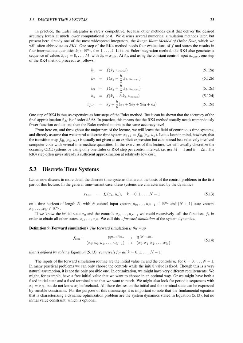
ii
“msi” — 2014/11/26 — 15:16 — page 35 — #35 ii
ii
ii
5.3. DISCRETE TIME SYSTEMS 35
In practice, the Euler integrator is rarely competitive, because other methods exist that deliver the desiredaccuracy levels at much lower computational cost. We discuss several numerical simulation methods later, butpresent here already one of the most widespread integrators, the Runge-Kutta Method of Order Four, which wewill often abbreviate as RK4. One step of the RK4 method needs four evaluations of f and stores the results infour intermediate quantities ki ∈ Rnx , i = 1, . . . , 4. Like the Euler integration method, the RK4 also generates asequence of values xj , j = 0, . . . ,M , with x0 = xinit. At xj , and using the constant control input uconst, one stepof the RK4 method proceeds as follows:
k1 = f(xj , uconst) (5.12a)
k2 = f(xj +h
2k1, uconst) (5.12b)
k3 = f(xj +h
2k2, uconst) (5.12c)
k4 = f(xj + h k3, uconst) (5.12d)
xj+1 = xj +h
6(k1 + 2k2 + 2k3 + k4) (5.12e)
One step of RK4 is thus as expensive as four steps of the Euler method. But it can be shown that the accuracy of thefinal approximation xM is of order h4∆t. In practice, this means that the RK4 method usually needs tremendouslyfewer function evaluations than the Euler method to obtain the same accuracy level.
From here on, and throughout the major part of the lecture, we will leave the field of continuous time systems,and directly assume that we control a discrete time system xk+1 = fdis(xk, uk). Let us keep in mind, however, thatthe transition map fdis(xk, uk) is usually not given as an explicit expression but can instead be a relatively involvedcomputer code with several intermediate quantities. In the exercises of this lecture, we will usually discretize theoccuring ODE systems by using only one Euler or RK4 step per control interval, i.e. use M = 1 and h = ∆t. TheRK4 step often gives already a sufficient approximation at relatively low cost.
5.3 Discrete Time Systems
Let us now discuss in more detail the discrete time systems that are at the basis of the control problems in the firstpart of this lecture. In the general time-variant case, these systems are characterized by the dynamics
xk+1 = fk(xk, uk), k = 0, 1, . . . , N − 1 (5.13)
on a time horizon of length N , with N control input vectors u0, . . . , uN−1 ∈ Rnu and (N + 1) state vectorsx0, . . . , xN ∈ Rnx .
If we know the initial state x0 and the controls u0, . . . , uN−1 we could recursively call the functions fk inorder to obtain all other states, x1, . . . , xN . We call this a forward simulation of the system dynamics.
Definition 9 (Forward simulation) The forward simulation is the map
fsim : Rnx+Nnu → R(N+1)nx
(x0;u0, u1, . . . , uN−1) 7→ (x0, x1, x2, . . . , xN )(5.14)
that is defined by solving Equation (5.13) recursively for all k = 0, 1, . . . , N − 1.
The inputs of the forward simulation routine are the initial value x0 and the controls uk for k = 0, . . . , N − 1.In many practical problems we can only choose the controls while the initial value is fixed. Though this is a verynatural assumption, it is not the only possible one. In optimization, we might have very different requirements: Wemight, for example, have a free initial value that we want to choose in an optimal way. Or we might have both afixed initial state and a fixed terminal state that we want to reach. We might also look for periodic sequences withx0 = xN , but do not know x0 beforehand. All these desires on the initial and the terminal state can be expressedby suitable constraints. For the purpose of this manuscript it is important to note that the fundamental equationthat is characterizing a dynamic optimization problem are the system dynamics stated in Equation (5.13), but noinitial value constraint, which is optional.
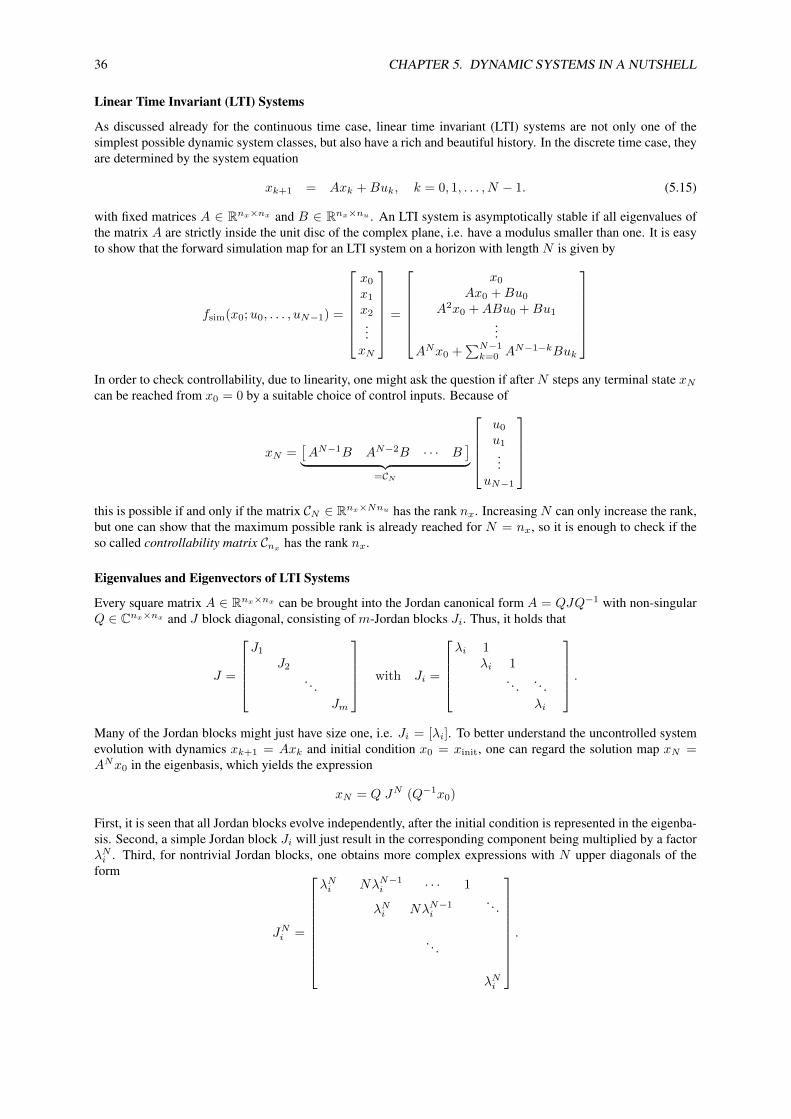
ii
“msi” — 2014/11/26 — 15:16 — page 36 — #36 ii
ii
ii
36 CHAPTER 5. DYNAMIC SYSTEMS IN A NUTSHELL
Linear Time Invariant (LTI) Systems
As discussed already for the continuous time case, linear time invariant (LTI) systems are not only one of thesimplest possible dynamic system classes, but also have a rich and beautiful history. In the discrete time case, theyare determined by the system equation
xk+1 = Axk +Buk, k = 0, 1, . . . , N − 1. (5.15)
with fixed matrices A ∈ Rnx×nx and B ∈ Rnx×nu . An LTI system is asymptotically stable if all eigenvalues ofthe matrix A are strictly inside the unit disc of the complex plane, i.e. have a modulus smaller than one. It is easyto show that the forward simulation map for an LTI system on a horizon with length N is given by
fsim(x0;u0, . . . , uN−1) =
x0
x1
x2
...xN
=
x0
Ax0 +Bu0
A2x0 +ABu0 +Bu1
...ANx0 +
∑N−1k=0 AN−1−kBuk
In order to check controllability, due to linearity, one might ask the question if after N steps any terminal state xNcan be reached from x0 = 0 by a suitable choice of control inputs. Because of
xN =[AN−1B AN−2B · · · B
]︸ ︷︷ ︸=CN
u0
u1
...uN−1
this is possible if and only if the matrix CN ∈ Rnx×Nnu has the rank nx. Increasing N can only increase the rank,but one can show that the maximum possible rank is already reached for N = nx, so it is enough to check if theso called controllability matrix Cnx has the rank nx.
Eigenvalues and Eigenvectors of LTI Systems
Every square matrix A ∈ Rnx×nx can be brought into the Jordan canonical form A = QJQ−1 with non-singularQ ∈ Cnx×nx and J block diagonal, consisting of m-Jordan blocks Ji. Thus, it holds that
J =
J1
J2
. . .Jm
with Ji =
λi 1
λi 1. . . . . .
λi
.Many of the Jordan blocks might just have size one, i.e. Ji = [λi]. To better understand the uncontrolled systemevolution with dynamics xk+1 = Axk and initial condition x0 = xinit, one can regard the solution map xN =ANx0 in the eigenbasis, which yields the expression
xN = Q JN (Q−1x0)
First, it is seen that all Jordan blocks evolve independently, after the initial condition is represented in the eigenba-sis. Second, a simple Jordan block Ji will just result in the corresponding component being multiplied by a factorλNi . Third, for nontrivial Jordan blocks, one obtains more complex expressions with N upper diagonals of theform
JNi =
λNi NλN−1i · · · 1
λNi NλN−1i
. . .
. . .
λNi
.
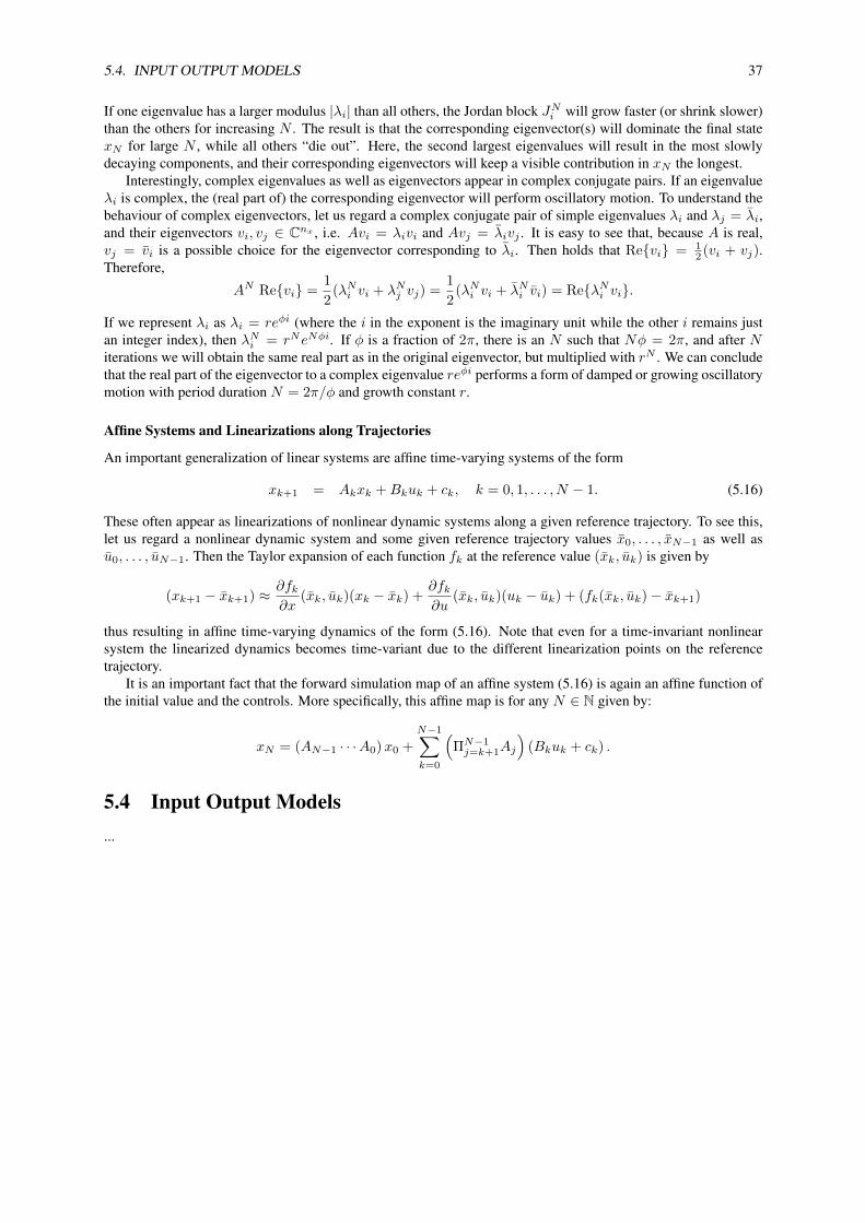
ii
“msi” — 2014/11/26 — 15:16 — page 37 — #37 ii
ii
ii
5.4. INPUT OUTPUT MODELS 37
If one eigenvalue has a larger modulus |λi| than all others, the Jordan block JNi will grow faster (or shrink slower)than the others for increasing N . The result is that the corresponding eigenvector(s) will dominate the final statexN for large N , while all others “die out”. Here, the second largest eigenvalues will result in the most slowlydecaying components, and their corresponding eigenvectors will keep a visible contribution in xN the longest.
Interestingly, complex eigenvalues as well as eigenvectors appear in complex conjugate pairs. If an eigenvalueλi is complex, the (real part of) the corresponding eigenvector will perform oscillatory motion. To understand thebehaviour of complex eigenvectors, let us regard a complex conjugate pair of simple eigenvalues λi and λj = λi,and their eigenvectors vi, vj ∈ Cnx , i.e. Avi = λivi and Avj = λivj . It is easy to see that, because A is real,vj = vi is a possible choice for the eigenvector corresponding to λi. Then holds that Re{vi} = 1
2 (vi + vj).Therefore,
AN Re{vi} =1
2(λNi vi + λNj vj) =
1
2(λNi vi + λNi vi) = Re{λNi vi}.
If we represent λi as λi = reφi (where the i in the exponent is the imaginary unit while the other i remains justan integer index), then λNi = rNeNφi. If φ is a fraction of 2π, there is an N such that Nφ = 2π, and after Niterations we will obtain the same real part as in the original eigenvector, but multiplied with rN . We can concludethat the real part of the eigenvector to a complex eigenvalue reφi performs a form of damped or growing oscillatorymotion with period duration N = 2π/φ and growth constant r.
Affine Systems and Linearizations along Trajectories
An important generalization of linear systems are affine time-varying systems of the form
xk+1 = Akxk +Bkuk + ck, k = 0, 1, . . . , N − 1. (5.16)
These often appear as linearizations of nonlinear dynamic systems along a given reference trajectory. To see this,let us regard a nonlinear dynamic system and some given reference trajectory values x0, . . . , xN−1 as well asu0, . . . , uN−1. Then the Taylor expansion of each function fk at the reference value (xk, uk) is given by
(xk+1 − xk+1) ≈ ∂fk∂x
(xk, uk)(xk − xk) +∂fk∂u
(xk, uk)(uk − uk) + (fk(xk, uk)− xk+1)
thus resulting in affine time-varying dynamics of the form (5.16). Note that even for a time-invariant nonlinearsystem the linearized dynamics becomes time-variant due to the different linearization points on the referencetrajectory.
It is an important fact that the forward simulation map of an affine system (5.16) is again an affine function ofthe initial value and the controls. More specifically, this affine map is for any N ∈ N given by:
xN = (AN−1 · · ·A0)x0 +
N−1∑k=0
(ΠN−1j=k+1Aj
)(Bkuk + ck) .
5.4 Input Output Models...

ii
“msi” — 2014/11/26 — 15:16 — page 38 — #38 ii
ii
ii
38 CHAPTER 5. DYNAMIC SYSTEMS IN A NUTSHELL

ii
“msi” — 2014/11/26 — 15:16 — page 39 — #39 ii
ii
ii
Bibliography
[Lju99] L. Ljung. System identification: Theory for the User. Prentice Hall, Upper Saddle River, N.J., 1999.
[Sch13] J. Schoukens. System identification, April 2013. Lecture Manuscript.
39