INSTITUT FOR MATEMATIK OG DATALOGISYDDANSK UNIVERSITET

Lecture Notes on Metric and TopologicalSpaces

Niels Jørgen Nielsen

2010

Introduction

The theory of metric and topological spaces is fundamental in most areas of mathematics and itsapplications. The study of concepts like convergence or continuity is essential in mathematicsand this theory puts these concepts into a general framework.

Most students know the basic properties of continuous functions defined on the real line, theplane or the space and the basic tool for defining and studying such functions is the ability ofmeasuring distances. We would like to put this into a more general setting. Assume e.g. thatwe have a set A of objects (this could be functions) each of which can be put into a system ofequations to give a solution. This creates a set B of solutions. The perfect situation is of coursethat if two objects in A are “close” the corresponding two solutions in B are also “close”.

The obstacle here is of course what we mean by “close”. If we in some way could define adistance function both on A and B, then we could also define what it means that two elementsin the given set are “close”. This is the background of defining a metric space which is a setequipped with a distance function, also called a metric, which enables us to measure the distancebetween two elements in the set.

It is however not always possible to find a reasonable metric (reasonable relative to our specificpurpose) on a given set, but then the more general concept of a topological space can often help.In such a space we use other ways to define what is means that two elements in the space areclose.

One of the mostly used tools in mathematics is compactness. A compact space is a topologicalspace where we loosely speaking have the ability to reduce a situation involving infinitely manyobjects of a certain type to a situation only involving finitely many objects.

The ability to perform compactness arguments is essential for anyone who wants to study math-ematics and its applications.

We now wish to discuss the arrangement of these notes in greater detail.

Section 0 contains some preliminaries on the concept of a function and some properties of thenatural numbers, the real numbers, and the complex numbers. Some readers might know thematerial presented here. Section 1 is devoted to inner product spaces which is a special case ofmetric spaces (and also cover the most important examples). This is done because many readersprobably have studied these spaces in a course on linear algebra. In section 2 we define metricspaces and investigate their basic properties while we in Section 3 prove some important theo-rems on continuous functions defined on metric spaces; these results have also applications tothe classical situation of real valued functions defined on an interval of R. In Section 4 we ex-tend our theory to general topological spaces and investigate continuous functions on topologicalspaces in Section 5. Section 6 is concerned with compact topological spaces, their properties,and how continuous functions behave on such spaces. We also give a proof of the classical theo-rem of Heine–Borel which characterizes the compact subsets of Rn. Section 7 contains the mostimportant results on connected subsets of topological spaces.

1

Though these notes are mainly on metric spaces, we have taken the attitude that if a notion is thesame for metric spaces and the more general topological spaces, then we use the more generalsetting. Similarly, if a proof of a result is more or less the same for metric and topological spaces,we give the proof in full generalty.

0 Notation and preliminaries

In these notes we shall use the following notation on the different sets of numbers:

• N denotes the set of natural numbers.

• Z denotes the set of integers.

• Q denotes the set of rational numbers.

• R denotes the set of real numbers.

• C denotes the set of complex numbers.

0.1 The concept of a function

Let X and Y be two sets. A function from X to Y is a relation which to every x ∈ X relatesa uniquely determined element in Y which is called f(x). X is called the domain of defintionfor f and Y is called the co–domain of f . That f is a function from X to Y , we shall write asf : X → Y . Once we have decided what X and Y should be, we will often just talk about thefunction f . If we change either the domain of definition, the relation f , or the co–domain, weget a new function. Let us now look on an example:

Example 0.1 Let f : R→ R be the function defined by f(x) = x2 for all x ∈ R. We could alsolook on the function g : [0, 1] → R defined by g(x) = x2 for all x ∈ [0, 1] or on the functionh : R → [0,∞[ defined by h(x) = x2 for all x ∈ R. Though the relation is the same, the threefunctions f , g, and h are different.

The image set of a function f : X → Y (or just the image of f ) is denoted by f(X) and is thesubset of Y defined by:

f(X) = {f(x) | x ∈ X}.

Note that we can consider f as a function from X to f(X) which is sometimes handy. Likewise,if A ⊆ X the image of A by f is the subset f(A) of Y defined by:

f(A) = {f(x) | x ∈ A}

A function f : X → Y is said to be injective if it satisfies the condition

∀x, y ∈ X : f(x) = f(y)⇒ x = y,

2

or equivalently∀x, y ∈ X : x 6= y ⇒ f(x) 6= f(y).

An injective function f is also called one–to–one and we shall often say f is 1–1 when we meanthat f is injective. f is called an injection.

A function f : X → Y is said to be surjective when f(X) = Y . Instead of saying that f issurjective we shall often say that f is onto and call f a surjection.

Whether a given f gives an injective or a surjective function depends heavily on which domainof definition or co–domain we use as the following simple example shows:

Example 0.2 If f : R → R is the function defined by f(x) = x2 for all x ∈ R, then f is neitherinjective nor surjective. If we change the function to (we shall still call it f ) f : [0,∞[→ R withf(x) = x2 for all x ∈ [0,∞[, then f becomes injective, but not surjective. If we finally considerf : [0,∞[→ [0,∞[, then f becomes both injective and surjective.

The function f : X → Y is said to be bijective if it is both injective and surjective. We then callf a bijection. f is a bijection if and only if

∀y ∈ Y ∃!x ∈ X : y = f(x),

where “∃!x” means that there exists exactly one x.

For a bijective f this statement can be used to define a function from Y to X , named f−1 : Y →X by the statement

∀y ∈ Y f−1(y) = x⇔ (x ∈ X) ∧ (f(x) = y).

f−1 is called the inverse function to f .

Unfortunately the symbol f−1 is also used when f is not bijective. If f : X → Y is any functionand V ⊆ Y , we put

f−1(V ) = {x ∈ X | f(x) ∈ V }.

The set f−1(V ) is called the inverse image of the set V by the function f .

In most cases this ambiguity does not cause problems as the following exercise hopefully shows.

Exercise 0.3 Let f : X → Y be a bijective function and call its inverse g : Y → X in thisexercise while we reserve the symbol f−1 to mean the inverse image by f . Prove that if V ⊆ Y ,then g(V ) = f−1(V ). this means in particular that if y ∈ Y , then g(y) = f−1({y}).

The inverse image construction is very essential and the next theorem gives a list of its basicproperties.

3

Theorem 0.4 Let f : X → Y be a function and let there for all i in an index set I be given aVi ⊆ Y . Further let V ⊆ Y and U ⊆ X . Then the following statements hold:

f−1(∅) = ∅ (0.1)f−1(Y ) = X (0.2)

f−1(Y \ V ) = X \ f−1(V ) (0.3)

f−1(⋃i∈I

Vi) =⋃i∈I

f−1(Vi) (0.4)

f−1(⋂i∈I

Vi) =⋂i∈I

f−1(Vi) (0.5)

f(f−1(V )) ⊆ V (0.6)f−1(f(U)) ⊇ U (0.7)

Exercise 0.5 Prove each of the statements in Theorem 0.4. Give examples where the inclusionsin the last two staments are sharp.

We used indexing in the formulation of the previous theorem so let us end this subsection byformalizing this concept.

Definition 0.6 Let I and A be two sets. A is said to indexed by I if there exists a bijectionf : I → A. Usually we shall put xi = f(i) for all i ∈ I and write A = {xi | i ∈ I} withoutmentioning f .

Indexing a set is a very practical notion; just look on the formulas in the previous theorem whichwould have been more complicated to write if we had not used indexing. Note also that there isno loss of generality to use it because any set can be indexed. Indeed, let A be any set and letId : A→ A be the identity function, that is Id(x) = x for all x ∈ A. Id is clearly a bijection sowe have indexed A by itself.

0.2 Sequences, countable sets and properties of N

We start with the following definition:

Definition 0.7 If A is an arbitrary set, then a sequence in A is a function f : N → A. Usuallywe will put xn = f(n) ∈ A for all n ∈ N and talk about the sequence (xn) without mentioningf .

Note that it is not required that the function f in Definition 0.7 is injective so some of the xn’smight be equal. It could happen that the {xn | n ∈ N} is finite. Consider e.g. the sequence(xn) ⊆ R defined by setting xn = 1 when n is even and xn = −1 when n is odd.

Definition 0.8 A set A is called countable if there is a bijection f : N→ A. In other words A isindexed by the natural numbers and we can with xn = f(n) for all n ∈ N write A = {xn | n ∈N}.

4

It is proved in [4, Exercises 10,12] that Z and Q are countable. An infinite set which is notcountable will be called uncountable. It will be proved later in these notes that R is uncountable.

A set is called at most countable if it is either finite or countable. Some authors also use the wordenumerable instead of countable.

Let us here mention one very important property of N which is the basis of the induction principle(proofs by induction).

The well ordering axiom for N

Every non–empty subset A of N has a minimal (smallest) element minA.

We now get the fundamental theorem on the induction principle:

Theorem 0.9 Let P (n) be an open statement involving one variable n from N. If

(i) The statement P (1) is true,

(ii) The statement (∀n ∈ N : P (n)⇒ P (n+ 1)) is true,

then the statement P (n) is true for all n ∈ N (or written with quatifiers: ∀n ∈ N P (n)).

Proof: We shall prove the theorem by contradiction so assume that P (n) is not true for all n ∈ Nwhis means that the set

A = {n ∈ N | P (n) is untrue} 6= ∅.

By the well ordering axiom for N the set A has a smallest element m. (i) implies that m > 1 sothat m − 1 ∈ N and hence by the choice of m P (m − 1) is true. Applying (ii) we get that thenalso P (m) is true which is a contradiction. 2

Proofs using Theorem 0.9 are called induction proofs or proofs by induction.

0.3 Properties of R

Some of the basic properties of R which we shall discuss in this part might be well known tosome of the readers.

Let S ⊆ R and let m,M ∈ R. M is called an upper bound for S if x ≤ M for all x ∈ S.Similarly m is called an lower bound for S if m ≤ x for all x ∈ S. S is called bounded fromabove if there exists an upper bound for S and similarly S is called bounded from below if it hasa lower bound. S is called bounded if it is bounded both from below and from above. Hence Sis bounded if and only if it is a subset of an interval [m,M ] of finite length.

We now need the following definition:

Definition 0.10 (Least upper bound) Let S ⊆ R and M0 ∈ R. M0 is called a least upper boundfor S, if

(i) M0 is an upper bound for S and

5

(ii) For every upper bound M for S we have that M0 ≤M .

Note that M0 is uniquely determined if it exists. Indeed, if M0 and M1 are least upper boundsfor S, then appying (ii) on M0, respectively M1 we get that M0 ≤ M1 and M1 ≤ M0; that isM0 = M1.

If S is not bounded from above, it has of course no least upper bound since (i) above cannot befulfilled. If S = ∅, every real number is an upper bound for S and hence (ii) cannot be fulfilled.Hence ∅ does not have a least upper bound.

It is a fundamental property of the real numbers that the empty set and the subsets of R whichare not bounded from above are the only subsets of R without a least upper bound. In these noteswe shall take this property as an axiom, but we will not make an axiomatic construction of R.

The completeness axiom of the real numbers

Every non–empty subset S ⊆ R which is bounded from above has a least upper bound. Thisnumber is uniquely determined and is called the supremum of S and written as supS.

It is important to notice that supS need not belong to S. If actually supS ∈ S, we shall writemaxS instead of supS. If S is unbounded from above and hence does not have a least upperbound, it is often convenient to put supS =∞.

Similar to Definition 0.10 we can define:

Definition 0.11 (Greatest lower bound) Let S ⊆ R and let m0 ∈ R. m0 is called a greatestlower bound for S if

(i) m0 is a lower bound for S and

(ii) For every lower bound m for S we have that m ≤ m0

Similar to the above it follows that m0 is uniquely determined if it exists.

If S ⊆ R, we put −S = {−x ∈ R | x ∈ S}. It is easily verified that m is a lower bound for S ifand only −m is an upper bound for −S and therefore we get from the completeness axiom:

Corollary 0.12 Every non–empty subset S ⊆ R which is bounded from below has a greatestlower bound. It is uniquely determined and is called the infimum of S and written inf S.

It follows of course that if S is bounded from below, then−S is bounded from above and inf S =− sup(−S). If inf S ∈ S, we shall write minS instead of inf S. If S is not bounded from belowit is convenient to put inf S = −∞.

As an application we can prove

Theorem 0.13 (Archimedes’ axiom)

The set N of natural numbers is not bounded from above.

Proof: We prove the theorem by contradiction so assume that N is bounded from above. Fromthe completeness axiom for R we get that a = sup N exists. If now n ∈ N is arbitrary, then

6

n+ 1 ∈ N and therefore n+ 1 ≤ a which gives that n ≤ a− 1. Since this holds for all n, a− 1is an upper bound for N, but this contradicts that a was the least upper bound. 2

The reason for the name of this theorem is that in some textbooks it is taken as one of the axiomsdefining N.

To make the reader more familar with the notions of sup and inf we prove the next theoremwhich will be used several times in these notes, in particular in Section 6.

Theorem 0.14 Let ([an, bn]) be a sequence of closed and bounded intervals so that [an+1, bn+1] ⊆[an, bn] for all n ∈ N. There exists a, b ∈ R with a ≤ b so that

∩∞n=1[an, bn] = [a, b]. (0.8)

Proof: Since [an, bn] ⊆ [a1, b1] for all n ∈ N we get that b1 is a upper bound for {an | n ∈ N}and that a1 is a lower bound for {bn | n ∈ N}. Therefore we can put

a = sup{an | n ∈ N}

andb = inf{bn | n ∈ N}

and we claim that these numbers are the required ones. To see this we first observe that since thesequence of intervals is decreasing, we get that for all n ≤ m an ≤ am < bm ≤ bn. Lookingon all the possible inequalities here we actually get that for all n,m ∈ N an ≤ bm. If we keepm fixed arbitrarily, this inequality shows that bm is an upper bound for the set {an | n ∈ N}and therefore a ≤ bm. Since this works for all m, we conclude that a is a lower bound for{bm | m ∈ N} and so a ≤ b. We have left to prove (0.8). Since a is an upper bound for (an)and b is a lower bound for (bn), we immediatelty get that an ≤ a ≤ b ≤ bn which shows that theinclusion “⊇” in (0.8) holds. To get the other inclusion we let x ∈ ∩∞n=1[an, bn] be arbitrary andget that an ≤ x ≤ bn for all n ∈ N. This inequality shows that x is and upper bound for (an) anda lower bound for (bn) and hence a ≤ x ≤ b, i.e x ∈ [a, b]. 2

Note that it can happen that a = b so that the interval [a, b] reduces to a point. In the exercisehours we will prove a much more general result [4, Exercise 5].

0.4 Properties of C

We recall that C is the plane where we have put i = (0, 1) so that every z ∈ C can be writtenas z = a + ib, where a, b ∈ R. a is called the real part of z and b is called the imaginary partof z and we write a = <z and b = =z. We add two complex numbers by adding their real andimaginary parts separately. Multiplication is defined so that i2 = −1 and if z = a1 + ib1 and

7

z2 = a2 + ib2, where a1, a2, b1, b2 ∈ R, then we multiply z1 with z2 as usual, just rememberingthat i2 = 1, that is

z1z2 = (a1 + ib1)(a2 + ib2) = (a1a2 − b1b2) + i(b1a2 + a1b2).

If again z = a + ib with a, b ∈ R, the number z = a − ib is called the complex conjugate of z.We easily get the following formulas:

z + z = 2a = 2<z

z − z = 2ib = 2i=z.

The number |z| = (a2 + b2)12 is called the the absolute value of z. It satisfies the following

conditions:

(i) zz = |z|2.

(ii) |z| ≥ 0 and |z| = 0⇔ z = 0.

(iii) For all z1, z2 ∈ C |z1z2| = |z1||z2|.

(iv) For all z1, z2 ∈ N |z1 + z2| ≤ |z1|+ |z2|

The following calculation shows (i):

zz = (a+ ib)(a− ib) = a2 − (ib)2 = a2 + b2 = |z|2.

(ii) is obvious and (iii) follows easily from (i) with z = z1z2. To obtain (iv) we first observe thatif z is written as above, then |z| = (a2 + b2)

12 ≥ |a| = |<z|. If now z1, z2 ∈ C, we use (i) to get:

|z1 + z2|2 = (z1 + z2)(z1 + z2) =

|z1|2 + |z2|2 + z1z2 + z2z1.

Since z1z2 = z1z2, we get from the above that

z1z2 + z1z2 = 2<(z1z2) ≤ |z1||z2|,

and inserting this we get that:

|z1 + z2|2 = |z1|2 + |z2|2 + 2<(z1z2) ≤|z1|2 + |z2|2 + 2|z1||z2| = (|z1|+ |z2|)2

and this shows (iv) which is called the triangle inequality.

In these notes we will develop a theory of topological spaces and will not use C very much sinceit turns out that as topological spaces C and R2 are identical. However, there are a few placeswhere it is convenient to use complex numbers.

8

0.5 From Logic: The Axiom of Choice

Here we discuss an axiom from Set Theory, called the Axiom of Choice which turns out to beindependent of the other more or less intuitive axioms from that theory. If we formulate it inordinary human language it sounds plausible and looks more like a trivial theorem:

The Axiom of Choice

If {Ai | i ∈ I} is an arbitrary family of non–empty sets, then we can choose a point in each ofthe Ai’s.

If we have to formulate this in a stringent mathematical way, we have to think about what itmeans “to choose”. This means that one has to give a rule how to choose so the mathematicalcorrect way of formulating the above is:

The Axiom of Choice

If {Ai | i ∈ I} is a family of non–empty sets, then there exists a function f : I → ∪i∈IAi so thatf(i) ∈ Ai for all i ∈ I .

The Axiom of Choice was first formulated in 1904 by Ernst Zermelo (1871–1956) and in 1940it was proved by Kurt Godel (1906–1978) that it is consistent with the other axioms from SetTheory (i.e the usual more or less “intuitive” axioms). Consistent means here that if we take theusual axioms and add the axiom of choice, then we get a logical system which does not containcontradictions. In 1963 it was proved by Paul Cohen (1934–2007) that the axiom of choice isindependent of the other axioms.

In the formulation above the axiom looks plausible and one has to think quite a bit to realizethat the existence of the function f does not follow trivially from the other axioms. It is howevermuch harder to accept some of the consequences of the axiom because some of them reallycontradict our intuition. We can for example mention that the axiom of choice implies that aball in R3 can be divided into finitely many peaces which you can put together to two balls, eachhaving the same volume as the original one! This follows from the fact that the axiom impliesthat there exists sets which cannot be given a volume and that such sets (the shape of which isbeyond our imagination) can be put together to something nice.

After a heavy debate in the 1930’s about the axiom of choice it is now accepted by most math-ematicians and in modern mathematics, a set theory which consists of the usual axioms and theaxiom of choice, is now used. This means that the axiom of choice is used in proofs without anyreference to it. This is also the case for these notes (see e.g.. the proof of Theorem 4.19 below).

The reason for the acceptance is probably that with a axiom system including the axiom of choiceas the foundation, one gets a mathematics the results of which are applicable to the existingworld. In particular in physics where Mathematical Analysis is used heavily and in this area ofmathematics one cannot avoid using the axiom of choice.

In the notes [6] written by this author there is a chapter on different equivalent formulations of

9

the axiom of choice. Let us end this section giving a simple equivalent formulation which cannotbe found in [6].

If X and Y are sets and g : X → Y is a function, then g is said to have a right inverse h if thereexists a function h : Y → X so that g(h(y)) = y for all y ∈ Y . We have the following theorem:

Theorem 0.15 The following statements are equivalent.

(i) The Axiom of Choice.

(ii) Every surjection has a right inverse.

Proof: (i) ⇒ (ii) : Assume (i) and let X and Y be given sets and g : X → Y be a surjection.Since g is surjective, g−1({y}) 6= ∅ for all y ∈ Y and therefore the axiom of choice gives a mapf : Y → ∪y∈Y g−1({y}) ⊆ X so that f(y) ∈ g−1({y}) for all y ∈ Y . Clearly g(f(y)) = y forall y ∈ Y so that f is a right inverse of g.

(ii) ⇒ (i) : Assume (ii) and let {Ai | i ∈ I} be an arbitrary family of non–empty sets. Weconsider the sets Ai × {i} ⊆ Ai × I and define X = ∪i∈I(Ai × {i}) ⊆ ∪i∈IAi × I . We notethat the sets Ai × {i} are mutually disjoint and therefore X is often called the disjoint union ofthe Ai’s; we also need the function p : ∪i∈IAi × I → ∪i∈IAi defined by p(x, i) = x for all(x, i) ∈ ∪i∈IAi × I . We now define a function g : X → I by

g(x, i) = i for all i ∈ I and all (x, i) ∈ Ai × {i}.

Note that g is well defined since the Ai×{i}’s are mutually disjoint. By (ii) g has a right inverseh : I → X which means that g(h(i)) = i for all i ∈ I . If we look on the definition of g, we seethat necessarily h(i) ∈ Ai×{i} for all i ∈ I . The function f : I → ∪i∈IAi defined by f = p ◦ hclearly has the property that f(i) ∈ Ai for all i ∈ I so that (i) is satisfied. 2

1 Normed vector spaces and inner product spaces

Some of the concepts we shall introduce in this section are well known from the course “LinearAlgebra” and some of the results we shall prove are also well known from that course. If X is avector space over C, we shall call X a complex vector space and if X is a vector space over R,we shall call X a real vector space. If it does not matter in the contents whether X is a real orcomplex vector space, we shall just write “vector space”.

We start by introducing the concept of length of a vector in an abstract vector space, namely theconcept of a norm.

Definition 1.1 Let X be a vector space. A function ‖ · ‖ : X → R is called a norm if it satisfiesthe following conditions:

N1 ‖x‖ ≥ 0 for all x ∈ X .

10

N2 ‖tx‖ = |t|‖x‖ for all x ∈ X and all t ∈ C, if X is a complex vector space (all t ∈ R if Xis a real vector space).

N3 ‖x+ y‖ ≤ ‖x‖+ ‖y‖ for all x ∈ X and all y ∈ Y .

N4 ∀x ∈ X : ‖x‖ = 0⇔ x = 0.

Remark: If we in N2 put x = 0 and t = 0, we get that ‖0‖ = 0 so the important implication inN4 is “⇒”. N3 is called the triangle inequality.If ‖ · ‖ is a norm on X , we shall call the pair (X, ‖ · ‖) a normed space. If it is clear from thecontents what the norm on X is, we shall simply talk about the normed space X .

The most obvious examples of normed spaces are of course R and C equipped with the absolutevalue of a number as the norm.

The most important normed spaces are Cn and Rn (where n ∈ N) equipped with their Euclidiannorm ‖ · ‖2 defined as follows: If x ∈ Cn with x = (x1, x2, · · · , xn), then

‖x‖2 = (n∑k=1

|xk|2)12 (1.1)

and similarly for x ∈ Rn. It requires however a bit of work and some additional results to seethat ‖ · ‖2 satisfies the triangle inequality when n > 1, so we start with a simpler example andpostpone the case of ‖ · ‖2 to a little later.

Example 1.2 Let n ∈ N and let X = Cn or X = Rn. If x ∈ X with x = (x1, x2, . . . , xn) wherexk ∈ C for all 1 ≤ k ≤ n (xk ∈ R if X = Rn), then we define ‖x‖1 by

‖x‖1 =n∑k=1

|xk|.

We have to show that ‖ · ‖1 is a norm on X . Since obviously it satisfies N1 and N2, we con-centrate on N3 and N4. To see that N3 is satisfied we let x = (x1, x2, · · · , xn) ∈ X andy = (y1, y2, · · · , yn) ∈ X and obtain

‖x + y‖1 =n∑k=1

|xk + yk| ≤

n∑k=1

|xk|+n∑k=1

|yk| = ‖x‖1 + ‖y‖1

where we have used that |xk + yk| ≤ |xk|+ |yk| for all 1 ≤ k ≤ n. This shows that N3 holds. If‖x‖1 = 0, then

n∑k=1

|xk| = ‖x‖1 = 0

and since all terms in the sum are non–negative, we get that xk = 0 for all 1 ≤ k ≤ n whichmeans that x = 0. Hence N4 is also satisfied.

11

A more complicated example is the following:

Example 1.3 let S be a set and define B(S,C) to be the set of all bounded functions f : S → C.If f, g ∈ B(S,C) and t ∈ C, we define the functions f + g;S → C and tf : S → C by

(f + g)(s) = f(s) + g(s) for all s ∈ S

(tf)(s) = tf(s) for all s ∈ S.‖f‖∞ = sup{|f(s)| | s ∈ S}

We wish to show that B(S,C) is a vector space and that ‖ · ‖∞ is a norm on B(S,C) (do notthink about the subscript∞; it is simply a tradition to use that subscript when a norm is definedby a supremum). Hence let t ∈ C, f, g ∈ B(S,C) be given. Since |f(s)| ≤ ‖f‖∞ for all s ∈ S,we get that |tf(s)| ≤ |t|‖f‖∞ which shows that tf is a bounded function, i.e. tf ∈ B(S,C). Itis also clear that

‖tf‖∞ = sups∈S|t||f(s)| = |t| sup

s∈S|f(s)| = |t|‖f‖∞

so that N2 is satisfied.

Since also |g(s)| ≤ ‖g‖∞ for all s ∈ S we get that

|f(s) + g(s)| ≤ |f(s)|+ |g(s)| ≤ ‖f‖∞ + ‖g‖∞ (1.2)

for all s ∈ S which gives that f + g ∈ B(S,C). It now follows that B(S,C) is a vectorspace under the addition and scalar multiplication given above. In addition (1.2) shows that‖f‖∞ + ‖g‖∞ is an upper bound for the set {|f(s) + g(s)| | s ∈ S} and since by definition‖f + g‖∞ is the least upper bound for that set we must have

‖f + g‖∞ ≤ ‖f‖∞ + ‖g‖∞

which shows that N3 is satisfied. If ‖f‖∞ = 0, then

|f(s)| ≤ ‖f‖∞ = 0 for all s ∈ S

which shows that f(s) = 0 for all s ∈ S so that f is the 0–function, that is the 0–vector inB(S,C). Since trivially N1 is satisfied, we have proved that ‖ · ‖∞ is a norm on B(S,C). Thespace B(S,R) can of course be treated similarly.

We now define inner products and inner product spaces which should be known from LinearAlgebra.

Definition 1.4 Let H be a complex vector space. A function (·, ·) : H × H → C is called aninner product on H if

∀x, y ∈ H : (x, y) = (y, x) (1.3)∀x, y, z ∈ H : (tx+ y, z) = t(x, z) + (y, z) (1.4)

∀x ∈ H : (x, x) ≥ 0 (1.5)(x, x) = 0 =⇒ x = 0. (1.6)

12

Remark: If H is a real vector space, then (x, y) ∈ R for all x, y ∈ H , and (1.3) then looks like

∀x, y ∈ H : (x, y) = (y, x). (1.7)

If H is a vector space with inner product (·, ·), we put ‖x‖ =√

(x, x) for all x ∈ H . Note that‖x‖ ≥ 0 for all x ∈ H and that ‖x‖ = 0 implies that x = 0. The pair (H, (·, ·)) is called an innerproduct space.

Example 1.5 Let n ∈ N. If x = (x1, x2, · · · , xn) ∈ Cn and y ∈ Cn we define

< x,y >=n∑k=1

xkyk

or if x,y ∈ Rn,

< x,y >=n∑k=1

xkyk.

< ·, · > is an inner product on Cn (Rn) and for all x ∈ Cn (for all x ∈ Rn) we have

‖x‖2 =< x,x >12

where ‖·‖2 is defined in (1.1). In the course Linear Algebra< x,y > was called the dot–productbetween x and y and denoted x · y. We shall not use the dot–notation here since the dot has atendency of disappearing in writing.

Exercise 1.6 Prove the statements in Example 1.5.

We shall now prove an important inequality for inner products which actually also will give that‖ · ‖ defined above is a norm.

Theorem 1.7 (Cauchy-Schwartz’ inequality)

If H is a vector space with inner product (·, ·), we have:

|(x, y)| ≤ ‖x‖‖y‖ for alle x ∈ H . (1.8)

Proof: If t ∈ R, x ∈ H og y ∈ H are arbitrary, we get that

0 ≤ (tx+ y, tx+ y) = t2‖x‖2 + t(x, y) + t(y, x) + ‖y‖2 (1.9)= t2‖x‖2 + t[(x, y) + (x, y)] + ‖y‖2

= ‖x‖2t2 + 2<(x, y)t+ ‖y‖2.

Put now p(t) = ‖x‖2t2 + 2<(x, y)t + ‖y‖2 for all t ∈ R. p is then a polynomium of degree 2which (1.9) satisfies p(t) ≥ 0 for all t ∈ R. Therefore p has a most one root which implies thatthe discriminand D of p is non–positive, hence

0 ≥ D = 4[<(x, y)]2 − 4‖x‖2‖y‖2. (1.10)

13

Dividing by 4 and taking the square root this gives

|<(x, y)| ≤ ‖x‖‖y‖. (1.11)

If H is a real vector space, (1.11) is the same as (1.8) and we have finished the proof in that case.If H is a complex vector space, we can continue as follows:

Put α = |(x,y)|(x,y)

if (x, y) 6= 0 and α = 1, if (x, y) = 0. Since |α| = 1 and |(x, y)| ≥ 0, (1.11)gives:

|(x, y)| = α(x, y) = (αx, y) = <(αx, y) ≤ ‖αx‖‖y‖ = |α|‖x‖‖y‖ = ‖x‖‖y‖, (1.12)

which exactly is (1.8). 2

We are now able to prove:

Theorem 1.8 If H is a complex or real vector space with inner product (·, ·) and we define‖x‖ = (x, x)

12 for all x ∈ H , then ‖ · ‖ is a norm on H .

Proof: We have to show that ‖ · ‖ satisfies N1–N4. N1 and N4 follows directly from (1.5) and(1.6). To prove N2 we let t ∈ C and x ∈ H be given arbitrarily. A little computation shows that

‖tx‖2 = (tx, tx) = tt‖x‖2 = |t|2‖x‖2 (1.13)

which proves N2.

Let x, y ∈ H be arbitrary. If we put t = 1 in (1.9) and apply the Cauchy–Schwartz’ inequalitywe get

‖x+ y‖2 = (x+ y, x+ y) = ‖x‖2 + ‖y‖2 + 2<(x, y) ≤ (1.14)‖x‖2 + ‖y‖2 + 2‖x‖‖y‖ = (‖x‖+ ‖y‖)2

and hence‖x+ y‖ ≤ ‖x‖+ ‖y‖

which proves the triangle inequality. 2

Corollary 1.9 ‖ · ‖2 as defined in (1.1) is a norm on Cn and Rn.

Proof: This follows directly from Theorem 1.8 and Example 1.5. 2

Let us finish this section with yet another example of an inner product space.

Example 1.10 Let a, b ∈ R with a < b and let C([a, b],C) denote the set of all continuousfunctions f : [a, b] → C. If we define sum and multiplication by scalars as in Example 1.3,C([a, b],C) becomes a complex vector space. If f, g ∈ C([a, b],C), we put

(f, g) =

∫ b

a

f(t)g(t)dt.

14

It is readily verified that (·, ·) is an innner product on C([a, b],C) and that the correspondingnorm is given by:

‖f‖2 = (

∫ b

a

|f(t)|2dt)12 for alle f ∈ C([a, b],C).

Exercise 1.11 Prove the statements in Example 1.10

2 Metric spaces and their topologies

In Section 1 we have seen how to define the lenght of a vector in a normed vector space, namelyas the norm of the vector. In this section we shall introduce so–called metric spaces where it ispossible to define distances between points. We start with:

Definition 2.1 Let S be a non–empty set. A function d : S × S → R is called a metric (or adistance function) if it satisfies the following conditions:

M1 d(x, y) ≥ 0 for all x, y ∈ S.

M2 d(x, y) = d(y, x) for all x, y ∈ S.

M3 d(x, y) ≤ d(x, z) + d(z, y) for all x, y, z ∈ S.

M4 ∀x, y ∈ S : d(x, y) = 0⇔ x = y

The pair (S, d) is called a metric space.

If you look on it intuitively M1, M2 and M4 are natural requirements for a distance function;the distance between two points should be non–negative, the distance from x to y should be thesame as the distance from y to x, and the distance between two points should be 0 if and onlyif they are equal. If you think about how you measure distances in the plane or in our physicalworld (3–dimensional space), you will also see that M3 is a natural requirement. M3 is calledthe triangle inequality.

If it is clear from the contents what the metric d is, we shall often write “the metric space S”instead of “the metric space(S, d)”.

Let us now look on some examples.

Example 2.2 Let S be any non–empty set and define d by d(x, y) = 1 if x, y ∈ S with x 6= yand d(x, y) = 0 if x, y ∈ S with x = y. It is clear from the definition that M1, M2 and M4 aresatisfied. To prove M3 we let x, y, z ∈ S be arbitrary. If x = y, then clearly

d(x, y) = 0 ≤ d(x, z) + d(z, y).

If x 6= y, then either x 6= z or z 6= y and hence

d(x, y) = 1 ≤ d(x, z) + d(z, y)

15

which shows that also M3 holds. Hence d is a metric on S. It is called the discrete metric on S.

This example is a bit exoctic, though sometimes useful. The next theorem will provide somemore important examples.

Theorem 2.3 If X, ‖ · ‖) is a normed space and d is defined by

d(x, y) = ‖x− y‖ for all x, y ∈ X,

then d is a metric on X turning it into metric space. d is called the metric induced by the normon X .

Proof: Let x, y, z ∈ X be arbitrary. By N1 d(x, y) = ‖x− y‖ ≥ 0 so M1 holds. By N2 we get

d(x, y) = ‖x− y‖ = ‖ − (y − x)‖ = ‖y − x‖ = d(y, x)

so M2 holds. By N3 we have

d(x, y) = ‖x− y‖ = ‖(x− z) + (z − y)‖ ≤ ‖x− z‖+ ‖z − y‖ = d(x, z) + d(z, y)

so that M3 holds. Finally N4 gives that d(x, y) = ‖x − y‖ = 0 if and only if x − y = 0, if andonly if x = y. Hence d is a metric on X . 2

Combining Theorem 2.3 with Theorem 1.8 we get that every inner product space is a metricspace in a natural manner. In particular Corollary 1.9 gives:

Corollary 2.4 Let n ∈ N. d2 defined by

d2(x, y) = ‖x− y‖2 for all x, y ∈ Cn (x, y ∈ Rn)

is a metric on Cn, respectively Rn.

d2 is called the Euclidian metric on Rn or Cn and is the one we will use on these spaces unlessotherwise stated. The reason is of course that this is the distance concept we normally use in reallife on R, R2, and R3. If we write it out in coordinates we get for all x = (x1, x2, · · · , xn) ∈ Cn

and all y = (y1, y2, · · · , yn) ∈ Cn:

d2(x,y) = (n∑k=1

|xk − yk|2)12 .

We could also use the norm ‖ · ‖1 from Example 1.2 to define a metric d1 on Cn or Rn. Indeed,if x and y are as above, then

d1(x,y) = ‖x− y‖1 =n∑k=1

|xk − yk|.

Any carpenter who is going to make a table for you will of course think that you are nuts ifyou insist that all measurements in R2 should be made using the metric d1. However, in some

16

mathematical proofs where metric spaces are applied , e.g. the proof of the existence of solutionsto certain differential equations, d1 is used instead of d2 of technical reasons: simply, no squareroots appear in the definition of d1. In the exercise hours you will see that d1 and d2 are equivalentmetrics (see the definition below).

In the rest of this section (S, d) will denote a fixed metric space.

If A ⊆ S is non–empty, we can consider the restriction dA of d to A× A, that is

dA(x, y) = d(x, y) for all x, y ∈ A.

Clearly dA is a metric on A and is called the metric on A induced by d. Thus any non–emptysubset of a metric space is itself a metric space with the induced metric. We shall not use thenotation dA much in the sequel, but will simply write d and remember that when we consider Aas a metric space, we only evaluate d in points in A× A. We shall also need:

Proposition 2.5 Let (X, dX) and (Y, dY ) be metric spaces. If x,y ∈ X × Y , say x = (x1, y1)and y = (x2, y2) where x1, x2 ∈ X and y1, y2 ∈ Y . If we put

d(x,y) = max{dX(x1, x2), dY (y1, y2)},

then d is a metric on X × Y .

If x ∈ S and r > 0, the set B(x, r) = {y ∈ S | d(x, y) < r} is called the ball with center xand radius r. We shall sometimes write the open ball with center x and radius r to emphasize thesharp inequality in a definition. B(x) is called a ball with center x if B(x) = B(x, r) for somer > 0. The closed ball with center x and radius r is the set Bc(x, r) = {y ∈ S | d(x, y) ≤ r}.

To illustrate that balls may look differently than anticipated given our intuition from Rn, we givethe following example:

Example 2.6 We consider Z ⊆ R with the metric induced by the metric on R. The ball withcenter 1 and radius 1 is

B(1, 1) = {n ∈ Z | |n− 1| < 1} = {1},

while the closed ball with center 1 and radius 1 is the set Bc(x, r) = {n ∈ Z | |n − 1| ≤ 1} ={0, 1, 2}.

We now introduce a very important concept.

Definition 2.7 A subset G ⊆ S is called open if for all x ∈ G there exists an r > 0 so thatB(x, r) ⊆ G. A subset F ⊆ S is called closed if S \ F is open.

As a quick example we see that an interval of the form ]a, b[ with a < b is an open subset of R. Ifwe in R2 let F be the line segment between the points (1, 2) and (3, 4) including the endpoints,F is a closed subset of R2. Make a drawing of the situation! If we let A be the same line segmentwithout the endpoints, A is neither open nor closed.

We need the following lemma which is a consequence of the triangle inequality.

17

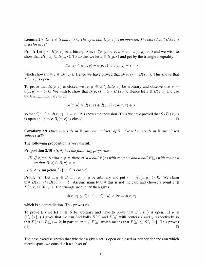
Lemma 2.8 Let x ∈ S and r > 0. The open ballB(x, r) is an open set. The closed ballBc(x, r)is a closed set.

Proof: Let y ∈ B(x, r) be arbitrary. Since d(x, y) < r, s = r − d(x, y) > 0 and we wish toshow that B(y, s) ⊆ B(x, r). To do this we let z ∈ B(y, s) and get by the triangle inequality:

d(x, z) ≤ d(x, y) + d(y, z) < d(x, y) + s = r

which shows that z ∈ B(x, r). Hence we have proved that B(y, s) ⊆ B(x, r). This shows thatB(x, r) is open.

To prove that Bc(x, r) is closed we let y ∈ S \ Bc(x, r) be arbitrary and observe that s =d(x, y) − r > 0. We wish to show that B(y, s) ⊆ S \ Bc(x, r). Hence let z ∈ B(y, s) and usethe triangle inequaly to get

d(x, y) ≤ d(x, z) + d(y, z) < d(x, z) + s

so that d(x, z) > d(x, y)−s = r. This shows the inclusion. Thus we have proved that S\Bc(x, r)is open and hence Bc(x, r) is closed. 2

Corollary 2.9 Open intervals in R are open subsets of R. Closed intervals in R are closedsubsets of R.

The following proposition is very useful.

Proposition 2.10 (S, d) has the following properties:

(i) If x, y ∈ S with x 6= y, there exist a ball B(x) with center x and a ball B(y) with center yso that B(x) ∩B(y) = ∅

(ii) Any singleton {x} ⊆ S is closed.

Proof: (i): Let x, y ∈ S with x 6= y be arbitrary and put r = 12d(x, y) > 0. We claim

that B(x, r) ∩ B(y, r) = ∅. Assume namely that this is not the case and choose a point z ∈B(x, r) ∩B(y, r). The triangle inequality then gives

d(x, y) ≤ d(x, z) + d(z, y) < 2r = d(x, y)

which is a contradiction. This proves (i).

To prove (ii) we let x ∈ S be arbitrary and have to prove that S \ {x} is open. If y ∈S \ {x}, (i) gives that we can find balls B(x) and B(y) with centers x and y respectively sothat B(x) ∩ B(y) = ∅; in particular x /∈ B(y) which means that B(y) ⊆ S \ {x}. This proves(ii). 2

The next exercise shows that whether a given set is open or closed or neither depends on whichmetric space we consider it a subset of.

18

Exercise 2.11 Let Z be equipped with the metric induced by R as in Example 2.6. Prove that{1} considered as a subset of Z is both open and closed. Prove next that if {1} is considered asa subset of R, then it is closed, but not open.

In higher dimensions it can often be difficult to decide whether a given set is open just by usingthe definition. In the next section we shall get some strong tools to decide that. Here we canprove:

Theorem 2.12 The following statements are satisfied.

(i) An arbitrary union of open subsets of S is open.

(ii) A finite intersection of open subsets of S is open.

(iii) An arbitrary intersection of closed subsets of S is closed.

(iv) A finite union of closed subsets of S is closed.

(v) S and ∅ are both open and closed.

Proof: To prove (i) we let I be an arbitrary index set and let {Gj | j ∈ I} be a family of opensubsets of S. We have to prove that G = ∪j∈IGj is open. If x ∈ G is given, there exists a j0 ∈ Iso that x ∈ Gj0 and since Gj0 is open, there exists an r > 0 with B(x, r) ⊆ Gj0 . This gives usimmediately that

B(x, r) ⊆ Gj0 ⊆ ∪j∈IGj = G

and hence G is open.

(ii): let n ∈ N and finitely many open subsets Hk ⊆ S, 1 ≤ k ≤ n be given and put H =∩nk=1Hk. We have to show that H is open so choose x ∈ H arbitrarily and observe that thisimplies that x ∈ Hk for all 1 ≤ k ≤ n. For each 1 ≤ k ≤ n Hk is open, and hence we can findan rk > 0 so that B(x, rk) ⊆ Hk. Put now r = min{rk | 1 ≤ k ≤ n} and note that since thereare only finitely many rk’s and r is the smallest of them, also r > 0. We claim that B(x, r) ⊆ H .If we fix a 1 ≤ k ≤ n, we get that B(x, r) ⊆ B(x, rk) ⊆ Hk. Since this holds for all 1 ≤ k ≤ nwe get that actually B(x, r) ⊆ ∩nk=1Hk = H . Thus we have proved that H is open.

(iv): Let I be an arbitrary index set and let {Fj | j ∈ I} be a family of closed subsets of S and putF = ∩k∈IFj . Since for each j ∈ I Fj is a closed set, S \ Fj is open. Standard set manipulationsgive us S \ F = ∪j∈I(S \ Fj) which is open by (i). Hence F is closed.

In a similar manner (iv) follows by taking complements and use (ii).

(v): Any ball with center in a point in S is by definition contained in S which shows that S isopen and hence ∅ is closed. ∅ is open since any statement that starts with “for all x ∈ ∅” is a truestatement. Therefore also S is closed. 2

If we take infinite intersections of open subsets of S, the conclusion in (ii) need not be true andsimilarly if we take infinite unions of closed subsets of S, the conclusion in (iv) need not be true.Here is an example:

19

Example 2.13 For every n ∈ N we consider the interval ]− 1n, 1n[⊆ R which is clearly open. We

claim that {0} = ∩∞n=1]− 1n, 1n[. Clearly “⊆” holds and if x ∈ ∩∞n=1]− 1

n, 1n[, then − 1

n< x < 1

n

for all n ∈ N so letting n → ∞, we obtain that x = 0. Hence the set equality above holds. But{0} is clearly not an open subset of R.

The example shows that even in the most simple cases the conclusion of (ii) in Theorem 2.12 isuntrue if we take infinite intersections. This means that one has to be very careful.

Let us define:Gd = {G ⊆ S | G is open in S}. (2.1)

Concepts that can be characterized solely using Gd are called topological concepts. We shall seebelow that many concepts are topological concepts though it apriori does not seem so. We needthe following definition:

Definition 2.14 Two metrics d and σ on S are called equivalent if they determine the same classof open sets, that is Gd = Gσ.

In the next result we denote balls in (S, d) by Bd and balls in (S, σ) by Bσ

Proposition 2.15 Two metrics d and σ are equivalent, if and only if

(i) ∀x ∈ S ∀Bd(x) ∃Bσ(x) : Bσ(x) ⊆ Bd(x),

(ii) ∀x ∈ S ∀Bσ1 (x) ∃Bd

1(x) : Bd1(x) ⊆ Bσ

1 (x).

Proof: Assume first that d and σ are equivalent. Let x ∈ S and a ball Bd(x) be given. Since thetwo metrics are equivalent, Bd(x) is open in (S, σ) and therefore there exists a ball Bσ(x) so thatBσ(x) ⊆ Bd(x). Hence (i) holds. By interchanging the roles of d and σ in this argument we get(ii).

Assume next that (i) and (ii) are satisfied and let G ∈ Gd be arbitrary. If x ∈ G we can bydefinition find a ball Bd(x) ⊆ G. By (i) we can find a ball Bσ(x) ⊆ Bd(x) ⊆ G. Since x ∈ Gwas arbitrary, we get that G is open in (S, σ), i.e G ∈ Gσ. Hence we have proved that Gd ⊆ Gσ.By interchanging the roles of d and σ and using (ii) we get the other inclusion. 2

As mentioned earlier we shall in the exercise hours see that on Cn and Rn the two metrics d1 andd2 are equivalent. Here we will give another example, but first we need a useful lemma.

Lemma 2.16 The following two statements are equivalent for a metric space (S, d):

(i) Every singleton is an open subset of S.

(ii) Every subset of S is open.

Proof: Assume first that (i) holds, that is {x} is open for all x ∈ S. If A ⊆ S is an arbitrarysubset, then clearly A = ∪x∈A{x}. Theorem 2.12 (i) now gives that A is open.

If (ii) holds, then every subset of S is open so in particular {x} is open for every x ∈ S. 2

20

Example 2.17 Let d denote the metric on Z induced by the usual metric on R as in Example2.6. In Exercise 2.11 we saw that {1} was open in (Z, d) and in the same way we can of courseget that {n} is open for every n ∈ Z. Using Lemma 2.16 we then get that every subset of Z isopen in (Z, d). Let σ be the discrete metric on Z as defined in Example 2.11. If n ∈ Z, thenBσ(n, 1) = {n} and hence {n} is open (Z, σ). Again Lemma 2.16 gives that every subset of Zis open in (Z, σ). This shows that d and σ are equivalent metrics on Z.

For sequences in metric spaces we have the following definition.

Definition 2.18 A sequence (xn) ⊆ S is said to converge to a point x ∈ S (notation: xn → xfor n→∞) if

∀ε > 0 ∃n0 ∈ N ∀n ∈ N : n ≥ n0 ⇒ d(x, xn) < ε. (2.2)

x is called the limit of (xn) or the limit point of (xn).

If xn → x for n → ∞, we shall often write x = limn→∞ xn which in particular is useful whena limit point occurs in some calculations. Instead of saying “(xn) converges to x” we shall oftensay “(xn) tends to x”.

Note also that since (2.2) must hold for all ε > 0, it does not matter whether we write “< ε” or“≤ ε”. Finally we observe that xn → x in S if and only if d(x, xn)→ 0 for n→∞.

Example 2.19 It is assumed well known to the reader that 1n→ 0 in R for n→∞ and this was

actually used in Example 2.13. If the reader is uncomfortable with this, here is a quick proof. Letε > 0 be arbitrarily given. By Theorem 0.13 there exists an n0 ∈ N so that n0 >

1ε

and hence ifn ≥ n0, 1

n≤ 1

n0< ε, which proves the statement.

We really need the following proposition.

Proposition 2.20 Any sequence (xn) ⊆ S has at most one limit point.

Assume that xn → x ∈ S and xn → y ∈ S for n→∞ and let ε > 0 be arbitrary. Since xn → x,there exists an n1 ∈ N so that d(x, xn) < ε for all n ≥ n1. Similarly, since xn → y, there existsan n2 ∈ N so that d(y, xn) < ε for all n ≥ n2. If we put m = max(n1, n2), then d(x, xm) < εsince m ≥ n1 and d(y, xm) < ε since m ≥ n2. The triangle inequality gives that

d(x, y) ≤ d(x, xm) + d(xm, y) < 2ε.

Since ε was arbitrary, we have proved that d(x, y) < 2ε for all ε > 0. Since the left hand side ofthis inequality does not depend on ε, we can let ε → 0 to obtain that d(x, y) = 0, hence x = y.2

We have the following proposition:

Proposition 2.21 Let (xn) ⊆ S be a sequence and let x ∈ S. xn → x if and only if:

∀U ∈ Gd with x ∈ U ∃n0 ∈ N : n ≥ n0 ⇒ xn ∈ U.

Consequently convergence of sequences in S is a topological property.

21

The last example of this section is based on Example 1.3:

Example 2.22 We let B([0, 1],C) denote the space of all bounded functions f : [0, 1] → Cequipped with the norm ‖ · ‖∞ as defined in Example 1.3. The corresponding metric d∞ isgiven by d∞(f, g) = ‖f − g‖∞ for all f, g ∈ B([0, 1],C). If we for every n ∈ N define thefunction fn(t) = 1

nt for all t ∈ [0, 1], then clearly 0 ≤ fn(t) ≤ 1

nfor all t ∈ [0, 1] so that

fn ∈ B([0, 1],C) with ‖fn‖∞ ≤ 1n

. Therefore d∞(fn, 0) = ‖fn‖∞ ≤ 1n→ 0 for n → ∞ and

fn → 0 in B([0, 1],C). This is actually not surprising.

3 Continuous functions on metric spaces

In this section we shall define continuous functions between metric spaces and investigate theirproperties.

We tacitly assume that the reader is familar with the continuity properties of the classical func-tions defined on the R or intervals of R. However, let us recall that if I ⊆ R is an interval andf : I → R is a function, then f is said to be continuous in a point x0 ∈ I , if

∀ε > 0 ∃δ > 0 ∀x ∈ I : |x− x0| < δ ⇒ |f(x)− f(x0)| < ε. (3.1)

Intuitively speaking, this means that when x gets close to x0, then f(x) gets close to f(x0). Ina metric space it has meaning to say that two points are close, namely if their distance is smalland therefore it has meaning to generalize (3.1) to metric spaces in order to define continuity offunctions between metric spaces. One should of course not generalize things for their own sake,but the reader will soon find that the concept of continuity of functions between metric spaces isextremely useful.

In the rest of this section we let (X, dX) and (Y, dY ) denote metric spaces

Definition 3.1 A function f : X → Y is said to be continuous in the point x0 ∈ X , if thefollowing condition holds:

∀ε > 0 ∃δ > 0 ∀x ∈ X : dX(x, x0) < δ ⇒ dY (f(x), f(x0)) < ε. (3.2)

f is said to be continuous if it is continuous in all points of X .

The reader is invited to compare equations (3.1) and (3.2) to check that (3.2) is really an extensionof (3.1).

Remark: If we let BX denote balls in X and BY denote balls in Y we get that (3.2) is equivalentto

∀BY (f(x0)) ∃BX(x0) : f(BX(x0)) ⊆ BY (f(x0)). (3.3)

Like in the case of functions from R to R one can check continuity by working with sequences.We have:

22

Theorem 3.2 Let f : X → Y be a function and x0 ∈ X . The following two statements areequivalent:

(i) f is continuous in x0.

(ii) For every sequence (xn) ⊆ X we have that if xn → x0, then f(xn)→ f(x0).

Proof: (i)⇒(ii): Assume (i) holds, let (xn) ⊆ X be an arbitrary sequence with xn → x0, andlet ε > 0 be arbitrary. Since f is continuous in x0, we can find a δ > 0 so that if x ∈ X withdX(x, x0) < δ, then dY (f(x), f(x0)) < ε. Further, since xn → x, there exists an n0 ∈ N sothat dX(x, xn) < δ for all n ≥ n0. If we now fix an arbitrary n ≥ n0, then dX(x0, xn) < δand therefore by the above dY (f(x0), f(xn)) < ε. Hence we have found an n0 so that whenevern ≥ n0, then dY (f(x0, f(xn)) < ε. This is exactly that f(xn)→ f(x0).

(ii)⇒(i): We assume that f is not continuous in x0 and have to find a sequence (xn) ∈ X sothat (xn) converges to x0, but (f(xn)) does not converge to f(x0). The discontinuity of f in x0

means that:

(∗) There exists an ε > 0 so that for all δ > 0 there exists an xδ ∈ X so that dX(x0, xδ) < δand dY (f(x0, xδ) ≥ ε.

Think this over!!

Since (∗) holds for all δ > 0, we can for an arbitrary n ∈ N, put δ = 1n

and (∗) will pro-vide us with an xn ∈ X , so that dX(x0, xn) <

1n

and dY (f(x0), f(xn)) ≥ ε. Think that overtoo!!. This gives us on one hand that dX(x0, xn) → 0 and hence xn → x0. One the other handdY (f(x0), f(xn)) ≥ ε for all n ∈ N so (f(xn)) does not converge to f(x0). Hence we haveproved what we wanted. 2

The next theorem is well known for classical continuous functions.

Theorem 3.3 Let (X, dX), (Y, dY ), and (Z, dZ) be metric spaces If f : X → Y is continuous inx0 ∈ X and g : Y → Z is continuous in f(x0) ∈ Y , then the composition g ◦ f is continuous inx0.

In particular, if f and g are continuous, then g ◦ f is continuous.

Proof: To prove it we shall apply Theorem 3.2. Let (xn) ∈ X be an sequence so that xn → x0.Since f is continuous in x0, f(xn) → f(x0), and since g is continuous in f(x0), g(f(xn)) →g(f(x0)). According to Theorem 3.2 this implies that g ◦ f is continuous in x0. 2

We now wish to prove a theorem which relates continuity to open sets. In fact, it turns out thatthe question of continuity of a given function f : X → Y is a topological property.

Theorem 3.4 Let f : X → Y be a function. The following three statements are equivalent:

(i) f is continuous.

23

(ii) For every open set G ⊆ Y f−1(G) is an open subset of X .

(iii) For every closed set F ⊆ Y f−1(F ) is a closed subset of X .

Proof: (i)⇒(ii): We assume that f is continuous and let G ⊆ Y be an arbitrary open subset.If f−1(G) = ∅, there is nothing to prove so assume that f−1(G) 6= ∅ and let x ∈ f−1(G) bearbitrary. We have to find a ball BX(x) with center x so that BX(x) ⊆ f−1(G).

Since f(x) ∈ G andG is open, we can find a ballBY (f(x)) with center f(x) so thatBY (f(x)) ⊆G. Since f is continuous in x, we can according (3.3) in the remark just after Definition 3.1 finda ball BX(x) so that f(BX(x)) ⊆ BY (f(x)) ⊆ G. Taking f−1 on both sides of this inequalitywe get that BX(x) ⊆ f−1(G) and we have proved what we wanted.

(ii)⇒(i): We assume (ii), let x ∈ X be arbitrary, and have to prove that f is continuous in x.If BY (f(x)) is an arbitrary open ball with center f(x), then by (ii) f−1(BY (f(x)) is an opensubset of X which clearly contains x. Therefore there exists a ball BX(x) with center x so thatBX(x) ⊆ f−1(BY (f(x)), or equivalently f(BX(x)) ⊆ BY (f(x)). (3.3) now gives that f iscontinuous in x.

To see that (ii)⇔(iii) we just observe that F ⊆ Y is closed in Y if and only if Y \ F is open andthat f−1(F ) = X \ f−1(Y \ F ) 2

Theorem 3.4 can alternatively be used to prove the second part of Theorem 3.3. Indeed, letf : X → Y and g : Y → Z be continuous. We wish to show that g ◦ f is continuous. Lettherefore G ⊆ Z be an arbitrary open set. Since g is continuous, g−1(G) is open in Y , and sincef is continuous, (g ◦ f)−1(G) = f−1(g−1(G)) is open in X , which by Theorem 3.4 implies thatg ◦ f is continuous.

Theorem 3.4 can also be used to prove that certain sets are open. Here is an example:

Example 3.5 A ⊆ R2 defined by:

A = {(x, y) ∈ R2 | arctan (x7y3 sin (x10y17 + 5)) + cos (x+ 5y) <1

100}

is an open subset of R2. To see this we define the function f : R2 → R by

f(x, y) = arctan (x7y3 sin (x10y17 + 5)) + cos (x+ 5y)

for all (x, y) ∈ R2. Since f is a composition of classical continuous functions, it is continuousand since the interval ]−∞, 1

100[ is open, we get that A = f−1(]−∞, 1

100[ is an open subset of

R2.

If f : X → Y is a continuous function, it is by definition continuous in all points of X and thiscan be written with quantifiers as:

∀ε > 0 ∀x ∈ X ∃δ > 0 ∀y ∈ X : dX(x, y) < δ ⇒ dY (f(x), f(y)) < ε. (3.4)

24

It is always a bit dangerous to interchange quantifiers in a logical statement because the statementchanges radically. Let us anyway look on the following statement:

∀ε > 0 ∃δ > 0 ∀x ∈ X ∀y ∈ X : dX(x, y) < δ ⇒ dY (f(x), f(y)) < ε. (3.5)

If we do a little text analysis of the two statements we see that in (3.4) the δ depends on ε andx while in (3.5) the δ only depends on ε and thus works for all x, y ∈ X . The statement (3.5)makes perfectly sence and gives rise to the following definition:

Definition 3.6 A function f : X → Y is called uniformly continuous if it satisfies (3.5).

The word “uniformly” is used because given ε > 0, one can use the same δ for all x, y ∈ X . Thenext statement is really an example, but we formulate it as a proposition.

Proposition 3.7 Let f : [1,∞[→ R be defined by f(x) =√x for all 1 ≤ x < ∞. Then f is

uniformly continuous.

Proof: Let x, y ≥ 1 be arbitrary. Since f is differentiable, we can by the mean value theoremfind a ξ between x and y so that

f(x)− f(y) = f ′(ξ)(x− y).

Since ξ ≥ 1 and f ′(ξ) = 12√ξ, we get that |f ′(ξ)| ≤ 1

2and hence

|f(x)− f(y)| ≤ 1

2|x− y|

which holds for all x, y ≥ 1. If now ε > 0 is arbitrary, we can choose a 0 < δ < 2ε and if|x− y| < δ, then by the above:

|f(x)− f(y)| ≤ ε.

This shows that f is uniformly continuous. 2

We shall later prove that any continuous function defined on a closed and bounded interval ofR is uniformly continuous. Combining this with Proposition 3.7 we get that the square rootfunction is in fact uniformly continuous on [0,∞[. The next example shows that even very nicecontinuous functions need not be uniformly continuous.

Example 3.8 let g : R → R be defind by g(x) = x2 for all x ∈ R. We claim that g is notuniformly continuous. It is clearly enough to prove that g is not uniformly continuous on [0,∞].To see this we put ε = 1 and let 0 < δ ≤ 1 be arbitrary. If x ≥ 0, we get

0 ≤ g(x+ δ)− g(x) = (x+ δ)2 − x2 = (2x+ δ)δ.

For all x > 12(δ−1 − δ) we get that

g(x+ δ)− g(x) > 1

which shows that g is not uniformly continuous.

25

4 Topological spaces

In many applications of mathematics one studies some objects which can be considered as ele-ments of a set X together with a system τ of subsets of X . We would then like to find a metricon X so that the open sets are precisely the sets belonging to τ . This is not always possible, butif the sets belonging to τ satisfies the same conditions as open sets do, then we are still able to dosomething, though we have to leave the metric situation. This is the background of this section.

If X is a set, we let P(X) denote the set of all subsets of X; that is

P(X) = {A | A ⊆ X}.

We make the following definition.

Definition 4.1 Let X be a set. A subset τ ⊆ P(X) is called a topology on X if the followingconditions are satisfied:

T1 If {Gi | i ∈ I} is an arbitrary system of subsets from τ , then

∪i∈IGi ∈ τ.

T2 If n ∈ N and Gk ∈ τ for 1 ≤ k ≤ n, then

∩nk=1Gk ∈ τ.

T3 ∅ ∈ τ and X ∈ τ .

Let us look on some examples:

Example 4.2 We shall here consider three examples.

• If we put τ = P(X), then obviously T1–T3 are satisfied, so P(X) is a topology on X . Itis called the discrete topology.

• If we put τ = {∅, X}, then we also get a topology on X , called the indiscrete topology.

• This example makes the connection to the previous sections. If (X, d) is a metric spaceand we put τ = Gd, then it follows from Theorem 2.12 that T1–T3 are satisfied. Hence Gdis a topology on X . It is called the topology generated by the metric d.

Definition 4.3 If τ is a topology on a set X , the pair (X, τ) is called a topological space. Thesubsets of X which are elements of τ are called the open subsets of the topological space (X, τ).A subset F ⊆ X is called closed if X \ F is open.

If there is no doubt about the topology on X we shall often in the sequel just write the “topolog-ical space X”.

Using the properties of taking complements the following proposition follows immediately fromDefinition 4.1 og Definition 4.3.

26

Proposition 4.4 If (X, τ) is a topological space, the following statements hold:

(i) Every intersection of closed sets is again closed.

(ii) Every finite union of closed sets is again closed.

(iii) X and ∅ are both open and closed.

It follows from Example 4.2 that every metric space is a topological space. A topological space(X, τ) is called metrizable if there exists a metric d on X , so that Gd = τ .

Proposition 4.5 Let X, τ) be a topological space and A ⊆ X . If we define τA ⊆ P(A) by

τA = {V = A ∩ U | U ∈ τ},

then τA is a topology on A. It is called the induced topology on A.

The proof is left to the reader.

Hence every subset A of a topological space is itself a topological space when we equip it withthe induced topology τA. We shall always use that topology when we consider a subset as atopological space. Note that if (X, d) is a metric space and A ⊆ X , then τA = GdA

where dA isthe induced metric on A as defined in Section 2.

We also need to be able to turn a product of two topological spaces into a topological space. Thisis the contents of the next proposition.

Proposition 4.6 Let (X, τ) and Y,S) be topological spaces. We define τX×Y be be the subset ofP(X × Y ) consisting af all sets of the form

∪i∈I(Ui × Vi),

where I is an arbitrary index set and Ui ∈ τ and Vi ∈ S are arbitrary for all i ∈ I . Then τX×Yis a topology on X × Y , called the product topology on X × Y .

Exercise 4.7 Prove Proposition 4.6.

If (X, dX) and (Y, dY ) are metric spaces, then it is readily verified that τX×Y = Gd where d isthe metric on X × Y defined in Proposition 2.5.

In the rest of this section we shall study topological spaces in greater detail and this investigationwill also give new results on metric spaces. In the rest of this section we let (X, τ) denote atopological space.

Definition 4.8 Let x ∈ X . A subsetM ⊆ X is called a neighbourhood of x if there exist an opensubset G ⊆ X with x ∈ G ⊆M . An open set G with x ∈ G is called an open neighbourhood ofx.

Note that according to the definition every non–empty open subset of X is a neighbourhood ofany of its points.

27

If x ∈ X , we shall in the sequel put

Ux = {U ⊆ X | U is a neighbourhood of x}

If (X, d) is a metric space we see that a subset M ⊆ X is a neighbourhood of a point x ∈ Xif and only if there exists a ball B(x) with center x so that B(x) ⊆ M . Due to this the onlyinteresting neighbourhoods of a point x in a metric space are the balls with center x. Our firstresult should be compared to Definition 2.7.

Theorem 4.9 A subset W ⊆ X is open if and only if every point x ∈ W has a neighbourhoodM with M ⊆ W .

Proof: If W is open in X , then it is a neigbourhood of any of its points x, so in this case we canput M = W for all x ∈ W .

Assume next that every x ∈ W has a neigbourhood Mx ⊆ W .By definition we can to everyx ∈ W find an open set Ux with x ∈ Ux ⊆Mx. If we can prove

W = ∪x∈XUx, (4.1)

we can conclude that W is open, since by T1 the right hand side of (4.1) is an open set. Toprove (4.1) we proceed af follows: By definition we have that Ux ⊆ W for all x ∈ X and hence∪x∈XUx ⊆ W . If z ∈ W , then z ∈ Uz ⊆ ∪x∈XUx which shows the other inclusion. 2

Definition 4.10 Let W ⊆ X . A point x ∈ W is called an inner point of W , if there exists aneighbourhood Ux of x so that Ux ⊆ W . The subset of W consisting of all innner points of W iscalled the interior of W and denoted int(W ).

It follows immediately that if (X, d) is a metric space and W ⊆ X , then a point x ∈ W is aninner point of W , if and only if there exists a ball B(x) with center x so that B(x) ⊆ W .

It can easily happen that W 6= ∅ while int(W ) = ∅. Let for example L be a line in the plane R2.If x ∈ L is any point, it is readily seen that every ball with center x will intersect R2 \ L so thatx is not an inner point. Hence int(L) = ∅.

We have the following result on the interior of a set.

Theorem 4.11 Let W ⊆ X . The following statements hold for int(W ):

(i) int(W ) is an open subset of X .

(ii) If U is an open subset of X with U ⊆ W , then U ⊆ int(W ).

(iii) int(W ) = ∪{U ⊆ W | U is open in X}.

Proof: (i): If int(W ) = ∅, there is nothing to prove so assume that int(W ) 6= ∅. If x ∈ int(W ),we can find an open neighbourhood U of x so that U ⊆ W . We wish to show that actuallyU ⊆ int(W ). To see this let y ∈ U be arbitrary. Since U is open, it is a neighbourhood of y andsince U ⊆ W , we get that y is an interior point of W . Hence U ⊆ int(W ).

28

Let us summarize what we have done. We started with a point x ∈ int(W ) and found an openneighbourhood U of x so that U ⊆ int(W ). An application of Theorem 4.9 now gives thatint(W ) is open. This proves (i).

(ii): Let U be an open subset of X so that U ⊆ W . If x ∈ U is arbitrary, then U is a neighbour-hood of x which by the above is fully contained in W . This shows that x ∈ int(W ). Hence wehave proved that U ⊆ int(W ).

(iii): Let V be equal to the union on the right hand side of (iii). Since V is a union of open sets,V is open and clearly V ⊆ W . By (ii) V ⊆ int(W ). Since int(W ) is open by (i), it is one ofthe U ’s that appear in the union on the right hand side of (iii) and therefore int(W ) ⊆ V . Thisshows the equality in (iii). 2

Together (i) and (ii) shows that int(W ) is the largest open subset of W .

We have the following corollary:

Corollary 4.12 A subset W ⊆ X is open if and only if W = int(W ).

Proof: If W is open, then by Theorem 4.11 (ii) W ⊆ int(W ), so W = int(W ). If we start withW = int(W ), then W is open since by Theorem 4.11 (i) int(W ) is open. 2

We now need the following definition:

Definition 4.13 Let A ⊆ X .

(i) A point x ∈ X is called a boundary point of A if every U ∈ Ux contains points from Aand from X \ A, that is U ∩ A 6= ∅ and U ∩ (X \ A) 6= ∅. The set of boundary points isdenoted by ∂A

(ii) A point x ∈ X is called a contact point ofA if everyU ∈ Ux intersectsA, that isU∩A 6= ∅.The set of contact points of A is denoted A and is called the closure of A.

(iii) A point x ∈ X is called an accumulation point ofA if for every U ∈ Ux (U \{x})∩A 6= ∅.

It follows immediately from the definition that every boundary point and every accumulationpoint belongs to A. So ∂A ⊆ A and A ⊆ A. Actually A = int(A) ∪ ∂A. This can be seen asfollows: If x ∈ A\int(A), then every U ∈ Ux intersectsA. On the other hand, since x /∈ int(A),we also have that every U ∈ Ux intersects X \ A and hence x ∈ ∂A.

The definition contains many concepts so therefore it is adequate to come with an example.

Example 4.14 Let A ⊆ R2 be defined by:

A = {(x, y) ∈ R2 | x2 + y2 < 1} ∪ {(1, 0)} ∪ {(2, 7)}.

A consists of the open disc with radius 1 and the points (1, 0) and (2, 7). If x = (x, y) withx2 + y2 ≤ 1 and B(x) is an arbitrary ball with center x, then B(x) ∩ A is an infinite set and

29

therefore in particular x is an accumulation point. The point (1, 0) is a boundary point whichactually belongs to A. If we take a ball with center (2, 7) and radius 1, it only intersects A in thepoint (2, 7). Hence (2, 7) is a contact point for A, but not an accumulation point. If x = (x, y)with x2 + y2 = 1, then clearly any ball with center x will intersect both A and R2 \ A, so x isa boundary point. Since (2, 7) ∈ A every ball with center (2, 7) of course intersects A, but it isalso clear that any ball with center (2, 7) intersects R2 \ A so (2, 7) is a boundary point of Awhich actually belongs to A. If x ∈ R2 with x2 + y2 > 1 and x 6= (2, 7), then it is also clear thatthere exists a ball with center x which does not intersect A. The conclusion is then that

A = {(x, y) ∈ R2 | x2 + y2 ≤ 1} ∪ {(2, 7)},

∂A = {(x, y) ∈ R2 | x2 + y2 = 1} ∪ {(2, 7)}

while the set of accumulation points of A is equal to

{(x, y) ∈ R2 | x2 + y2 ≤ 1}.

We have the following result on the closure A of a subset A of the toplogical space X:

Theorem 4.15 If A ⊆ X , the following statements hold:

(i) A is a closed set.

(ii) If F ⊆ X is a closed set with A ⊆ F , then A ⊆ F .

(iii) A = ∩{F ⊂ X | A ⊆ F F closed}.

Proof: (i): We have to prove that X \ A is open so let x ∈ X \ A be arbitrary. Since x /∈ A, xis not a contact point for A and therefore there is an open U ∈ Ux so that U ∩ A = ∅. We claimthat actually U ∩ A = ∅. If namely there exists a z ∈ U ∩ A, then z is a contact point for A andsince U is open, it is a neigbourhood of z which implies that U ∩A 6= ∅. This is a contradiction.Hence U ∩ A = ∅ which means that U ⊆ X \ A. Hence X \ A is open.

(ii): Let F be a closed subset of X with A ⊆ F . We shall prove (ii) by contradiction so assumethat A \ F 6= ∅ and choose a point z in that set. Since z ∈ X \ F , which is open, there exists aneigbourhood U of z so that U ⊆ X \ F . But z is a contact point for A, so U ∩A 6= ∅. This is acontradiction, since A ⊆ F and U ∩ F = ∅.

(iii): Since A is closed by (i), it is one of the sets in the intersection on the right hand side of(iii) and hence A contains that intersection. On the other hand, if F is a closed subset of X withA ⊆ F , then by (ii) A ⊆ F . Therefore A is contained in the intersection on the right hand sideof (iii). This proves (iii). 2

As a corollary we obtain:

Corollary 4.16 If A ⊆ X , then A is closed if and only if A = A.

30

Proof: If A = A, then A is closed because A is closed by Theorem 4.15 (i). If on the other handA is closed, (ii) of that theorem shows that A ⊆ A and hence A = A. 2

The use of Corollary 4.16 is the most common way to prove that a given set A is closed.

We also need:

Theorem 4.17 If A ⊆ X and B ⊆ X , then we have:

(i) A ∪B = A ∪B.

(ii) A ∩B ⊆ A ∩B.

Proof: (i): Since A ∪ B ⊆ A ∪ B and the latter set is closed, we get from Theorem 4.15(i)that A ∪B ⊆ A ∪ B. The theorem also clearly gives that A ⊆ A ∪B and B ⊆ A ∪B henceA ∪B ⊆ A ∪B. This proves (i).

(ii): Since A ∩ B ⊆ A ∩ B and the latter set is closed we get again from Theorem 4.15 thatA ∩B ⊆ A ∩B. 2

One cannot expect equality in Theorem 4.17 (ii). Indeed, let us consider the subsets A = [0, 1[and B =]1, 2] of R. Since A ∩ B = ∅, also A ∩B = ∅. On the other hand A = [0, 1] andB = [1, 2] so that A ∩B = {1}.

We now wish to define convergence of sequences in topological spaces in the same way as wedid for metric spaces.

Definition 4.18 Let (xn) ⊆ X and let x ∈ X . We say that (xn) converges (or tends to) x(notation: xn → x), if

∀U ∈ Ux ∃n0 ∈ N : n ≥ n0 ⇒ xn ∈ U.

This definition is clearly a generalization of Definition 2.18 for metric spaces.

Theorem 4.19 Let A ⊆ X and let x ∈ X . Consider the statements:

(i) There exists a sequence (xn) ⊆ A so that xn → x.

(ii) x ∈ A.

If (X, τ) is a general topological space, then (i) implies (ii). If (X, d) is a metric space, then (i)and (ii) are equivalent.

Proof: Let us first consider the case of a general topological space. If (xn) ⊆ A with xn → x,we have to show that x ∈ A. Hence let U ∈ Ux be arbitrary. Since xn → x, there is an n0 ∈ Nso that xn ∈ U for all n ≥ n0. But then {xn | n ≥ n0} ⊆ U ∩A so that U ∩A 6= ∅ which showsthat x ∈ A

Let now (X, d) be a metric space. We have to prove that (ii) implies (i) so let x ∈ A be arbitrary.Since x is a contact point for A, B(x, 1

n) ∩ A 6= ∅ for all n ∈ N and therefore we can choose a

31

sequence (xn) so that xn ∈ B(x, 1n) ∩ A for all n ∈ N. This sequence is a sequence from A and

since d(x, xn) ≤ 1n

, we get that d(x, xn)→ 0 which means that xn → x. 2

In general topological spaces (ii) does not imply (i).

As a corollary we get

Corollary 4.20 If A ⊆ R is an upper bounded and closed subset, then supA ∈ A. Similarly, ifB ⊆ R is a lower bounded and closed set, then inf B ∈ B.

Proof: If n ∈ N is arbitrary, supA − 1n

is not an upper bound for A and therefore there existsan xn ∈ A so that supA − 1

n< xn ≤ supA. Clearly xn → supA and therefore supA ∈ A by

Theorem 4.19, but since A is closed A = A. Similarly for the set B. 2

The next result on metric spaces explains the name accumulation point.

Theorem 4.21 If A is a subset of a metric space (X, d) and x is an accumulation point of A,then every ball with center x (or for that matter every neighbourhood of x) contains infinitelymany points from A.

Proof: Let R > 0 be arbitrary. By induction we will construct a sequence (xn) ⊆ B(x,R) ∩ Aso that xn 6= xm for all n,m ∈ R with n 6= m and xn 6= x for all n. Since x is an accumulationpoint of A, there is an x1 ∈ B(x,R) ∩ A with x1 6= x. Assume next that we have constructed{xk | 1 ≤ k ≤ n} ⊆ B(x,R) ∩ A so that they are all different and different from x. Sinced(x, xk) > 0 for all 1 ≤ k ≤ n, we can find an 0 < r < R with r < d(x, xk) for all 1 ≤ k ≤ n.Again since x is an accumulation point, there is an xn+1 ∈ B(x, r) ∩ A with xn+1 6= x. Clearlyd(x, xn+1) < d(x, xk) when 1 ≤ k ≤ n so xn+1 6= xk and since r < R we also get thatxn+1 ∈ B(x,R) ∩ A. This finishes the induction. Since all the xn’s are different we have foundinfinitly many points in B(x,R) ∩ A. 2

The reason for that the above proof works is of course that in metric spaces we can separatepoints with balls. There is nothing in the definition of a topological space which can give us asimilar separation of points by neigbourhoods. This is the background of the next definition.

Definition 4.22 X is called a Hausdorff space, if there for all x, y ∈ X with x 6= y exists aU ∈ Ux and a V ∈ Uy with U ∩ V = ∅.

It follows from Propossition 2.10 that all metric spaces are Hausdorff spaces. Most of the spacesyou will meet will be Hausdorff spaces. Similar to Theorem 4.21 we get:

Theorem 4.23 If A is a subset of a Hausdorff space X and x is an accumulation point of A,then every neighbourhood of x contaions infinitely many points from A.

Proof: We will try to mimic the proof of Theorem 4.21 so let U ∈ Ux be an arbitrary openneighbourhood (it is enough to consider open neighbourhoods). By induction we shall construct

32

a sequence (xn) ⊆ U ∩ A, so that xn 6= x and xn 6= xm for all n,m ∈ N, n 6= m.

Since x is an accumulation point for A, there exists an x1 ∈ U ∩ A with x 6= x1

Assume next that we have constructed {xk | 1 ≤ k ≤ n}, fulfilling our conditions. By theHausdorff property we can for every 1 ≤ k ≤ n find an open neigborhood Vk of x so thatxk /∈ Vk. If we put V = U ∩ ∩nk=1Vk, then V is an open neighbourhood of x, not containingany of the xk’s and with V ⊆ U . Again since x is an accumulation point for A, we can find anxn+1 ∈ V ∩ A which is different from x. This finishes the induction.

Since all the xn’s are different, we have found infinitely many points in U ∩ A. 2

Notice that in the proof we have only used the Hausdorff property to conclude that X has asomewhat weaker property; namely that if two points in X are different, then each of the pointshas a neighborhood not containing the other point. This property is called T1, but we shall notuse it in these notes. The stronger Hausdorff property is more important to us.

It is practical to know the next result:

Proposition 4.24 A sequence in a Hausdorff space has at most one limit point.

Proof: Let (xn) be a sequence in a Hausdorff space (X, τ) and assume that there are x, y ∈ Xso that xn → x and xn → y and x 6= y. By the Hausdorff property we can find a U ∈ Ux and aV ∈ Uy with U ∩ V = ∅. Since xn → x, there is an n1 ∈ N so that xn ∈ U for all n ≥ n1 andsince xn → y, there is an n2 ∈ N so that xn ∈ V for all n ≥ n2. If we put n = max{n1, n2},then xn ∈ U ∩ V which is a contradiction. 2

Let us end this section by a few results on so–called dense subsets of topological spaces. Westart with the definition.

Definition 4.25 A subset A of the topological space X is said to be dense in X if A = X .

The definition immediately implies the next proposition.

Proposition 4.26 A subset A of X is dense if and only if every non–empty open subset of Xcontains at least one point of A.

Proof: Left to the reader. 2

Definition 4.27 X is called separable if it contains a countable dense subset.

Let us end this section with two important result on very concrete topogical spaces.

Theorem 4.28 The set Q of rational numbers is dense in the set R of real numbers. In particularR is separable.

33

Proof: It is clearly enough to show that any bounded open interval ]a, b[ contains points fromQ and since 0 ∈ Q we need only consider the cases a ≥ 0 or b ≤ 0 (it is actually enough toconsider intervals of length less than one. Why?).

Assume that a ≥ 0 and choose n ∈ N so that n > (b−a)−1. Since the setB = {k ∈ N | an < k}is non–empty, it contains a first elementm. We claim that a < m

n< b. To see this we observe that

by the definition of B we get a < mn

and since m is the first element in B, then either m− 1 = 0orm−1 ∈ N\B. In both cases we get that m−1

n≤ a and hence m

n= m−1

n+ 1

n< a+(b−a) = b.

Hence we have proved that mn∈]a, b[.

If b ≤ 0, we can use the map x → −x to move the interval ]a, b[ to the non–negative part of R,apply the first case, and then go back.

Hence we have proved that Q = R and since Q is countable by [4, Exercise 12], we concludethat R is separable. 2

You can think about the proof of Theorem 4.28 as follows: After having chosen n ∈ N with1n< b − a you walk along the real line starting in 0 and take steps of length 1

n. Since your step

length is strictly smaller than the interval length, you have to hit the interval ]a, b[ after a finitenumber of steps.

Theorem 4.28 can be generalized to Rn. Indeed, if one does the above proof on each coordinatewe get the following:

Theorem 4.29 If n ∈ N, then Qn is dense in Rn. In particular Rn is separable.

The fact that Qn is countable can be established by applying induction on the Exercises 11 and12 in [4].

The importance of the notion of density comes in the situation where you have to check whethera given topological space has a certain property; in many cases it is enough to check that a densesubset has the property in question.

5 Continuous functions on topological spaces

In this section we will generalize the concept of continuity to functions between topologicalspaces and obtain some additional results on continuity which also cover the case of metricspaces. We start with the following definition which is a generalization of Definition 3.1, seealso equation (3.3) in the remark just after.

Definition 5.1 Let X and Y be topological spaces, and x0 ∈ X . A function f : X → Y is saidto be continuous in x0, if the following condition holds:

∀V ∈ Uf(x0) ∃U ∈ Ux0 : f(U) ⊆ V. (5.1)

f is said to be continuous if it is continuous in every x0 ∈ X .

34

Our first theorem should be compared to Theorem 3.2:

Theorem 5.2 LetX and Y be topological spaces, x0 ∈ X , and f : X → Y a function. Considerthe statements:

(i) f is continuous in x0.

(ii) For all sequences (xn) ⊆ X we have that if xn → x0, then f(xn)→ f(x0).

In general (i) implies (ii). If X is a metric space, (i) and (ii) are equivalent.

Proof: The proof looks much as that of Theorem 3.2. Assume first that (i) holds, let (xn) ⊆ Xbe a sequence with xn → x0, and let V ∈ Uf(x0) arbitrary. The continuity of f gives us a U ∈ Ux0

so that f(U) ⊆ V . Since xn → x0, there is an n0 ∈ N so that xn ∈ U for all n ≥ n0, but thenalso f(xn) ∈ V for all n ≥ n0. This shows that f(xn)→ f(x0).

In the case where (X, d) is a metric space, we assume that f is discontinuous in x0 and have toprove that (ii) does not hold. The discontinuity of f in x0 means:

(∗) there exists a V ∈ Uf(x0) so that for all δ > 0 there exists an xδ ∈ X with d(x0, xδ) < δand f(xδ) /∈ V .

Since (∗) holds for all δ > 0, we can for every n ∈ N put δ = 1n

and (∗) will provide us withan xn ∈ X so that d(x0, xn) <

1n

and f(xn) /∈ V . Since d(x0, xn) → 0, xn → x0, but sincef(xn) /∈ V for any n, (f(xn)) cannot converge to f(x0). This shows that (ii) does not hold. 2

The next theorem is a generalization of Theorem 3.3.

Theorem 5.3 Let X , Y , and Z be topological spaces and x0 ∈ X . If f : X → Y g : Y → Z sothat f is continuous in x0 and g is continuous in f(x0), then g ◦ f is continuous in x0.

In paticular, if f and g are continuous, then g ◦ f is continuous.

Proof: Let W ∈ Ug(f(x0)) be arbitrary. Since g is continuous in f(x0), there is a V ∈ Uf(x0) withg(V ) ⊆ W and since f is continuous in x0, there is a U ∈ Ux0 with f(U) ⊆ V . If now x ∈ U ,we get that f(x) ∈ V and that g(f(x)) ∈ W . Hence we have proved that (g ◦ f)(U) ⊆ W andthe continuity of g ◦ f in x0 is established. 2

Now we generalize Theorem 3.4.

Theorem 5.4 Let X and Y be topological spaces and f : X → Y a function. The followingstatements are equivalent.

(i) f is continuous.

(ii) For every open subset G ⊆ Y f−1(G) is an open subset X .

(iii) For every closed subspace F ⊆ Y f−1(F ) is a closed subspace of X .

35

Proof: (i) ⇒ (ii): We assume that f is continuous and let G ⊆ Y be an arbitrary open subsetof Y . If f−1(G) = ∅, there is nothing to prove so assume f−1(G) 6= ∅ and let x ∈ f−1(G) bearbitrary. We have to find a U ∈ Ux with U ⊆ f−1(G).

Since f(x) ∈ G and G is open, G is a neighbourhood of f(x) and the continuity of f providesus with a U ∈ Ux so that f(U) ⊆ G which is equivalent to U ⊆ f−1(G). This shows that (i)implies (ii).

(ii) ⇒ (i) : We assume (ii), let x ∈ X be arbitrary, and have to show that f is continuous in x.Hence let V be an arbitrary open neighbourhood of f(x) and put U = f−1(V ). Since x ∈ U andU is open by (ii), U is a neighbourhood of x. Clearly f(U) ⊆ V . This shows (i).

The equivalence of (ii) and (iii) can be proved exactly as in Theorem 3.4. 2

We end this section with a useful application.

Theorem 5.5 Let X and Y be topological spaces and assume that Y is a Hausdorff space. Iff, g : X → Y are continuous, the set {x ∈ X | f(x) 6= g(x)} is open.

Proof: Put A = {x ∈ X | f(x) 6= g(x)}and let x ∈ A be arbitrary. Since f(x) 6= g(x) and Y isa Hausdorff space, we can find open neighbourhoods V ∈ Uf(x) and W ∈ Ug(x) with V ∩W = ∅and since f and g are continuous, f−1(V ) and g−1(W ) are open. Clearly x ∈ f−1(V )∩ g−1(W )so that this set is an open neighbourhood of x. If z ∈ f−1(V ) ∩ g−1(W ), then f(z) ∈ V andg(z) ∈ W so that f(z) 6= g(z) This shows that f−1(V )∩ g−1(W ) ⊆ A and hence that A is open.2

Corollary 5.6 Let X and Y be as in Theorem 5.5 and let B be a dense subset of X .If f, g : X → Y are continuous and f(x) = g(x) for all x ∈ B, then f = g.

Proof: Since f and g are continuous, the set {x ∈ X | f(x) = g(x)} is closed by Theorem 5.5and contains B by assumption. Therefore

Y = B ⊆ {x ∈ X | f(x) = g(x)}

which shows that f(x) = g(x) for all x ∈ X , i.e. f = g. 2

6 Compact sets

This section is probably the most important in these notes because we shall here define thenotion of compactness which is applied vastly in all areas of mathematics. Let us discuss thearrangement of this section in greater detail. First we prove two classical results concerningclosed and bounded intervals of R and from these we draw some consequences about real–valued continuous functions defined on closed and bounded intervals of R. Inspired by the

36

classical results we define compact subsets of topological spaces and prove many deep resultson the structure of such sets and how continuous functions behave on them. After this we returnto the classical case and use the general theory to give a complete description of the compactsubsets of Rn for all n ∈ N.

We need some new notions in this section. This is included in the following definition.

Definition 6.1 Let X be a topological space and A ⊆ X . A family C of subsets of X is said tobe a cover of A if

A ⊆⋃G∈C

G.

If every G ∈ C is open, C is called an open cover of A.

A subcover of G is a subfamily D ⊆ C so that D is still a cover of A.

In the connection with covers we shall also use terms like “C covers A” or “the G’s from C coverA”.

6.1 Two classical results

We start with a lemma which sharpens Theorem 0.14.

Lemma 6.2 If ([an, bn]) is a sequence of closed and bounded intervals so that [an+1, bn+1] ⊆[an, bn] for all n ∈ N, we have:

(i) There exists a, b ∈ R with a ≤ b so that∞⋂n=1

[an, bn] = [a, b]. (6.1)

(ii) If in addition the interval length bn − an → 0 for n→∞, then a = b and hence∞⋂n=1

[an, bn] = {a}

Proof: (i) is clearly the same as Theorem 0.14 so we only have to prove (ii). Hence assume thatbn − an → 0. Since the sequence of intervals is decreasing, we get as in the proof of Theorem0.14 that an ≤ am < bm ≤ bn for all n ≤ m so that (an) is an increasing sequence and (bn) isdecreasing. We also saw that

a = sup{an | n ∈ N}b = inf{bn | n ∈ N}.

Since (an) is increasing, it follows from [5, Exercise 13] that an → a and the same exercise alsogives that bn → b. Hence bn − an → b− a so that a = b. 2

We are now able to prove:

37

Theorem 6.3 (Weierstrass’ accumulation theorem)Let a, b ∈ R with a < b. Every infinite subset A ⊆ [a, b] has at least one accumulation point in[a, b].

Proof: Let A ⊆ [a, b] be an infinite set. By successive division of an interval in the middle weshall by induction construct a sequence ([an, bn]) of closed and bounded intervals so that

(i) A ∩ [an, bn] is an infinite set for all n ∈ N.

(ii) [an+1, bn+1] ⊆ [an, bn] ⊆ [a, b] for all n ∈ N.

(iii) bn+1 − an+1 = 12(bn − an) for all n ∈ N.

For n = 1 we put a1 = a and b1 = b and it follows from our assumption that [a1, b1] satisfies ourconditions (only (i) is relevant in the first step of the induction).

Let now n ≥ 1 and assume that we have constructed the intervals [ak, bk] for all 1 ≤ k ≤ nso that (i)–(iii) are satisfied. We then have to construct the (n + 1)th interval. This is done asfollows:

We divide the interval [an, bn] in the middle and get the two intervals [an,an+bn

2] and [an+bn

2, bn].

By intersecting with A we get

A ∩ [an, bn] = (A ∩ [an,an + bn

2]) ∪ (A ∩ [

an + bn2

, bn]).

Since by the induction hypothesis the set on the left side of this equality is infinite, at least oneof the sets forming the union on the right side must also be infinite. If A ∩ [an,

an+bn2

] is infinite,we put an+1 = an and bn+1 = an+bn

2and if it is finite, we put an+1 = an+bn

2and bn+1 = bn. In

both cases the interval [an+1, bn+1] will satisfy (i)–(iii). Hence we have constructed the sequenceof intervals.

Iterating (iii) we obtain that bn − an = 2−n+1(b− a) so that bn − an → 0 and hence by Lemma6.2 we get an x ∈ [a, b] with

∞⋂n=1

[an, bn] = {x}.

We wish to show that x is an accumulation point for A. Let therefore r > 0 be arbitrary.We saw in Lemma 6.2 that both sequences (an) and (bn) tend to x for n → ∞ and hencewe can find n1, n2 so that x − r < an for all n ≥ n1 and bn < x + r for all n ≥ n2.If we now put n = max{n1, n2}, we obtain that [an, bn] ⊆]x − r, x + r[ and hence alsoA ∩ [an, bn] ⊆ A∩]x − r, x + r[. Since by construction A ∩ [an, bn] is an infinite set, it fol-lows that also A∩]x− r, x+ r[ is infinite. Since this holds for all r > 0, x is accumulation pointfor A. 2

The next important classsical result we shall prove is the following:

38

Theorem 6.4 (Heine–Borel)Let a, b ∈ R with a < b. Every open cover of [a, b] has a finite subcover.

Proof: We shall prove the theorem by contradiction so assume that C is an open cover of [a, b]without a finite subcover. We will reach a contradiction using the same technique as in the proofof Theorem 6.3. By induction we shall construct a sequence ([an, bn]) of bounded and closedintervals so that

(i) For no n ∈ N can [an, bn] be covered by finitely many G’s from C.

(ii) [an+1, bn+1] ⊆ [an, bn] ⊆ [a, b] for all n ∈ N.

(iii) bn+1 − an+1 = 12(bn − an) for all n ∈ N.

For n = 1 we put a1 = a and b1 = b.

Let now n ≥ 1 and assume that we have constructed the intervals [ak, bk] for all 1 ≤ k ≤ n sothat (i)–(iii) are satisfied. To construct the interval [an+1, bn+1] we proceed as follows:

Since by assumption [an, bn] cannot be covered by finitely many G’s from C at least one of theintervals [an

an+bn2

] and [an+bn2

, bn] cannot be covered by finitely manyG’s from C. If this happensto the first mentioned interval, we put an+1 = an and bn+1 = an+bn

2, else we choose the other

interval and get that [an, bn] satisfies (i)–(iii). This finishes the induction.

As in the proof of Theorem 6.3 we get that bn − an → 0 and hence there is an x ∈ [a, b] so that

∞⋂n=1

[an, bn] = {x}.

Since C is a cover of [a, b], there is a G ∈ C so that x ∈ G and since G is open, G is a neigh-bourhood of x and therefore there is an r > 0 with ]x− r, x+ r[⊆ G. Since as before both (an)and (bn) tend to x, there is an n0 ∈ N so that an, bn ∈]x − r, x + r[ for all n ≥ n0; in particular[an0 , bn0 ] ⊆]x− r, x+ r[⊆ G.

Hence we have obtained that a single G from G covers [an0 , bno ] which contradicts (i). 2

Some of the readers might know the next theorem, but have probably never seen a proof of it.It is a consequence of the results we have obtained so far and the proof illustrates quite well thetechniques to be used in this section.

Theorem 6.5 Let a, b ∈ R with a < b. If f : [a, b] → R is continuous, then f is bounded; i.e.there exists a K > 0 so that |f(x)| ≤ K for all x ∈ [a, b].

Proof: Since f is continuous we can for every x ∈ [a, b] find a δx > 0 so that |f(y)− f(x)| ≤ 1for all y ∈ [a, b] with |y− x| < δx (we use here the continuity condition with ε = 1). Hence also|f(y)| ≤ |f(y) − f(x)| + |f(x)| ≤ 1 + |f(x)| for all y ∈ [a, b] with |y − x| < δx. Clearly thesystem

C = {]x− δx, x+ δx[ | x ∈ X}

39

is an open cover of [a, b] and therefore it follows from Theorem 6.4 that there exist finitely manypoints x1, x2, · · · , xn ∈ [a, b] so that

[a, b] ⊆n⋃j=1

]xj − δxj, xj + δxj

[. (6.2)

PutK = max{|f(xj)| | 1 ≤ j ≤ n}+ 1.

We claim that |f(x)| ≤ K for all x ∈ [a, b]. If namely x ∈ [a, b] is arbitrary, then according to(6.2) there exists a 1 ≤ j ≤ n so that x ∈]xj − δxj

, xj + δxj[ and hence

|f(x)| ≤ |f(x)− f(xj)|+ |f(xj)| ≤ 1 + |f(xj)| ≤ K.

2

We could also have used Theorem 6.3 to prove Theorem 6.5. We shall a little later strengthenTheorem 6.5 considerably.

The last theorem of this subsection marks a small detour from our theme, but we have includedit here because it is important and because its proof resembles those of the Theorem 6.3 and 6.4.

Theorem 6.6 The set R of real numbers is uncountable.

Proof: Let (xn) ⊆ R be an arbitrary sequence with xn 6= xm for all n,m ∈ N with n 6= m. Ifwe can prove that

R 6= {xn | n ∈ N}, (6.3)

it will follow that R is uncountable. To achieve this we will by induction construct a sequence([an, bn]) of closed and bounded intervals so that

(i) xn /∈ [an, bn] for all n ∈ N,

(ii) [an+1, bn+1] ⊆ [an, bn] for all n ∈ N,

(iii) bn+1 − an+1 = 13(bn − an).

For n = 1 we choose a bounded interval [a1, b1] so that x1 /∈ [a1, b1]. Let next n ≥ 1 and assumethat we have constructed the intervals [ak, bk] for all 1 ≤ k ≤ n so that (i)–(iii) are satisfied. Ifwe divide [an, bn] in three intervals of equal length, at least one of these will not contain xn+1

so choose this and call it [an+1, bn+1]. Clearly our conditions are satisfied. This finishes theinduction.

Since bn − an → 0, we get from Lemma 6.2 that there exists an x ∈ R so that

{x} =∞⋂n=1

[an, bn].

If n ∈ N is arbitrary, then x ∈ [an, bn] while xn /∈ [an, bn] which shows that x 6= xn. This proves(6.3). 2

40

6.2 Compactness and sequentially compactness

In this subsection we let X denote a topological space.

Inspired by the two classical results above we give the following two definitions:

Definition 6.7 A subsetK ⊆ X is called compact if every open cover ofK has a finite subcover.

Definition 6.8 A subset K ⊆ X is called sequentially compact if every infinite subset of K hasan accumulation point in K.

In the defintion it is important that the accumulation point belongs to K.

From Theorem 6.3 and Theorem 6.4 we get immediately:

Corollary 6.9 Every closed and bounded interval of R is both compact and sequentially com-pact.

In general we have:

Theorem 6.10 Every compact subset of X is sequentially compact.

Proof: Let K ⊆ X be compact. It is clearly equivalent to prove that any subset of K without anaccumulation point in K is finite so let A ⊆ K be a subset without any accumulation point in K.Hence if x ∈ K, there exists an open Ux ∈ Ux so that Ux ∩A = {x} if x ∈ A and Ux ∩A = ∅ ifx /∈ A. We have clearly that

K ⊆⋃x∈K

Ux

so that {Ux | x ∈ K} is an open cover of K. Since K is compact, there exists a finite set ofpoints, say {xj | 1 ≤ j ≤ n ⊆ K} so that

K ⊆n⋃j=1

Uxj

and if we intersect with A, we get

A = A ∩K ⊆n⋃j=1

(Uxj∩ A).

Each of the sets in the union above contains at most one element and therefore the union is afinite set and hence also A is finite. 2

We shall a bit later prove that in metric spaces compactness and sequentially compactness areequivalent notions but let us begin by investigating compactness a little. The first result is easy,but quite useful.

Theorem 6.11 If X is compact, every closed subset of X is also compact.

41

Proof: Let K ⊆ X be closed and let C be an open cover of K, that is

K ⊆⋃G∈C

G,

from which we get thatX =

⋃G∈C

G ∪ (X \K). (6.4)

Since K is closed, X \K is open and therefore (6.4) shows that C ∪ {X \K} is an open coverof X . Since X is compact, we can find finitely many G1, G2, · · · , Gn ∈ C so that

X =n⋃j=1

Gj ∪ (X \K),

but taking intersection with K we get from this that

K ⊆n⋃j=1

Gj.

Hence we have found a finite subcover of C which shows that K is compact. 2

The next theorem is somewhat in the other direction.

Theorem 6.12 Let X be a Hausdorff space and let K ⊆ X be compact. If x ∈ (X \K), thenthere exist open sets U and V so that x ∈ U , K ⊆ V , and U ∩ V = ∅.

In particular K is closed.

Proof: Since X is a Hausdorff space, we can to every y ∈ K find open sets Uy and Vy so thaty ∈ Vy, x ∈ Uy, and Uy ∩ Vy = ∅. Clearly

K ⊆⋃y∈K

Vy

so that {Vy | y ∈ K} is an open cover ofK which by the compactness ofK has a finite subcover,say {Vj | 1 ≤ j ≤ n}. If we put U = ∩nj=1Uj and V = ∪j=1Vj , then U and V are both openwith x ∈ U and K ⊆ K. We claim that U ∩ V = ∅. Indeed, for every 1 ≤ j ≤ n we haveU ∩ Vj ⊆ Uj ∩ Vj = ∅ and therefore U ∩ V = ∪nj=1(U ∩ Vj) = ∅. Hence we have proved thefirst part of the theorem.

To prove the second part we observe that if x ∈ (X \ K) and U is constructed as above, thenU is a neighbourhood of x with U ⊆ (X \K). Since this works for all x ∈ (X \K), we haveproved that X \K is open and hence K is closed. 2

42

If X is not a Hausdorff space, there exist points x, y ∈ X which cannot be separated by opensets and since singletons clearly are compact sets, the first part of Theorem 6.12 is false in thiscase. If X is not a T1–space, there are singletons which are not closed so also the second part ofthe theorem is false.

The following definition and proposition are often handy:

Definition 6.13 A subset K ⊆ X is said to have the finite intersection property if the followingcondition is satisfied:

For every family F of closed subset of X with K ∩ ∩F∈FF = ∅ there exist an n ∈ N andF1, F2, · · · , Fn ∈ F with K ∩ ∩nj=1Fj = ∅.

For a proof of the next propostion see [4, Exercise 20].

Proposition 6.14 If K ⊆ X , the following two statements are equivalent.

(i) K is compact.

(ii) K has the finite intersection property.

As a corollary we get the following result which is often used in existence proofs.

Corollary 6.15 If K ⊆ X is compact and F is a family of closed subsets of X so thatK ∩ ∩F∈Ff

F 6= ∅ for all finite subfamilies Ff of F , then K ∩ ∩F∈FF 6= ∅.

Let us now look a little on the metric situation. We need the following definition:

Definition 6.16 A subsetK of a metric space (X, d) is called bounded if it is a subset of an openball in X .

If we for K ⊆ X define diam(K) = sup{d(x, y) | x, y ∈ K}, then it easily follows from thetriangle inequality that K is bounded if and only if diam(K) <∞.

Note also that boundedness of a set in a metric space is not a topological property, but dependson the specific metric d. Indeed, if (X, d) is a metric space, we can according to [4, Exercise 4]find an equivalent metric d′ on X so that d′(x, y) ≤ 1 for all x, y ∈ X and hence every subset ofX will be bounded with respect to d′.

Theorem 6.17 In a metric space (X, d) every compact subspace is closed and bounded.

Proof: Let K ⊆ X be compact and let x0 ∈ X . Since

K ⊆ X =∞⋃k=1

B(x0, k),

the family {B(x, k) | k ∈ N} is an open cover of K and therefore there exists an n ∈ N so that

K ⊆n⋃k=1

B(x0, k) = B(x0, n)

43

which shows that K is bounded.

It follows from Theorem 6.12 that K is closed. 2

In a general metric space a closed and bounded subset need not be compact. Indeed, if we definethe metric d′ from [4, Exercise 4], then R is closed and bounded in that metric, but R is clearlynot compact.

However, if we equip Rn with the usual metric, then a subset of Rn is compact if and only if itis closed and bounded. This result is called the Theorem of Heine–Borel and is one of the mostimportant theorems of these notes. The theorem will be proved in the next subsection.

We shall now look on sequential compactness, in particular in metric spaces. We need the fol-lowing:

Definition 6.18 Let (xn) ⊆ X be a sequence. If (nk) ⊆ N with nk < nk+1 for all n ∈ N, then(xnk

) is called a subsequence of (xn).

Here is a trivial lemma which readers often forget to take into account.

Lemma 6.19 If (xn) ⊆ X and the set {xn | n ∈ N} is finite, then (xn) has a constant subse-quence (xnk

). In particular (xnk) is convergent.

Proof: Since the finite set A = {xn | n ∈ N} is indexed by the infinite set N there must be ana ∈ A so that N1 = {n ∈ N | xn = a} is an infinite set. If we number N1 by a sequence (nk)with nk < nk+1 for all k ∈ N, we get that xnk

= a for all k. A constant sequence is clearlyconvergent. 2

We are now able to give the following characterization of sequentially compact subsets of metricspaces.

Theorem 6.20 Let K be a subset of the metric space (X, d). The following statements areequivalent.

(i) K is sequentially compact.

(ii) Every sequence (xn) ⊆ K has a convergent subsequence with limit point in K.

Proof: (i) ⇒ (ii): Let K ⊆ X be sequentially compact and let (xn) ⊆ K be a sequence.Because of Lemma 6.19 it is no loss of generality to assume that the set A = {xn | n ∈ N} isinfinite and therefore A has an accumulation point x ∈ K. By induction we shall construct asubsequence (xnk

) of (xn) so that

xnk∈ B(x,

1

k) for all k ∈ N. (6.5)

Since x is an accumulation point for A we can choose a point xn1 ∈ B(x, 1).

44

Assume next that k ≥ 1 and that we have constructed {xnj| 1 ≤ j ≤ k} so that (6.5) holds.

Since by Theorem 4.21 the set B(x, 1k+1

) ∩ A is infinite, we can find a nk+1 > nk so thatxnk+1

∈ B(x, 1k+1

). This finishes the induction.

It follows from (6.5) that d(x, xnk)→ 0 so that xnk

→ x. This proves (i)⇒ (ii).

(ii) ⇒ (i): Assume that (ii) holds and let D be an infinite subset of K. We have to prove thatD has an accumulation point in K. Since D is infinite, we can find a sequence (xn) ⊆ D withxn 6= xm for all n 6= m which then by assumption has a convergent subsequence (xnk

) withx = limk xnk

∈ K. If B(x) is any ball with center x, there is a k0 ∈ N so that xnk∈ B(x) for

all k ≥ k0. Since the xnk’s are mutually different, this means that B(x) contains infinitely many

points from D so that x is an accumulation point of D. 2

Note that we used the Axiom of Choice in (i)⇒ (ii).

The next theorem which states that compactness and sequentially compactness are equivalentnotions in metric spaces is one of our main theorems.

Theorem 6.21 If K is a subset of the metric space (X, d), the following statements are equiva-lent.

(i) K is compact.

(ii) K is sequentially compact

For general topological spaces (ii) need not imply (i).

The proof of Theorem 6.21 is technically somewhat difficult and we need two lemmas before wecan give the proof.

Lemma 6.22 If (xn) is a sequence in a metric space (X, d) and there is an r > 0 so thatd(xn, xm) ≥ r for all n 6= m, then (xn) has no convergent subsequences.

Proof: Assume that (xn) has a convergent subsequence (xnk) with limit x. Hence we can find a

k0 ∈ N so that d(x, xnk) < r

2for all k ≥ k0. If now k, j ≥ k0 with k 6= j, then by the triangle

inequalityd(xnk

, xnj) ≤ d(xnk

, x) + d(x, xnj) < r

which contradicts our assumptions on the sequence (xn). 2

The next lemma is more involved:

Lemma 6.23 Let K be a sequentially compact subset of a metric space (X, d). If C is an opencover of K, there exists an r > 0 so that there for all x ∈ K exists a U ∈ C with B(x, r) ⊆ U .

Proof: For every n ∈ N we define

An = {x ∈ K | B(x,1

n) \ U 6= ∅ for all U ∈ C} (6.6)

45

and claim that there is a m ∈ N so that Am = ∅.

To prove this claim by contradiction we assume thatAn 6= ∅ for all n ∈ N and choose an xn ∈ Anfor all n. Since K is sequentially compact, there exist by Theorem 6.20 a subsequence (xnk

) andan x0 ∈ K so that xnk

→ x0. Since C is a cover of K, there is a U0 ∈ C with x0 ∈ U0 andsince U0 is open, there is an ε > 0 with B(x0, ε) ⊆ U0. Let us choose k0 so that n−1

k0< ε

2. Since

xnk→ x0, we can find a k1 so that

d(xnk, x0) <

ε

2for all k ≥ k1.

We now put k = max{k0, k1} and claim thatB(xnk, n−1

k ) ⊆ B(x0, ε). Indeed, if y ∈ B(xnk, n−1

k ),then

d(y, x0) ≤ d(y, xnk) + d(xnk

, x0) < n−1k +

ε

2≤ ε

which shows that y ∈ B(x0, ε). Summarizing we have proved that

B(xnk, n−1

k ) ⊆ B(x0, ε) ⊆ U0

which clearly contradicts that xnk∈ Ank

.

Hence we have proved that there is an m ∈ N so that Am = ∅. We claim that r = m−1 is thenumber we are looking for. Indeed, if x ∈ K is arbitrary, then of course x /∈ Am and by thedefinition of Am there is a U ∈ C so that B(x,m−1) ⊆ U . 2

Note that the important information in the lemma of course is that the number r does not dependon the points x ∈ K but only on the covering C of K.

The reader will also observe that the Axiom of Choice was used in the proof.

We are finally ready for:

Proof of Theorem 6.21: It follows from Theorem 6.10 that (i) implies (ii) for all topologicalspaces so we only need to prove that (ii) implies (i) which we want to do by contradiction. If Kis sequentially compact and not compact, we can find an open cover C of K which does not havea finite subcover and let r be the number from Lemma 6.23. By induction we shall construct asequence (xn) ⊆ K so that for all n ∈ N we have:

xn+1 /∈n⋃k=1

B(xk, r) (6.7)

For n = 1 we just pick some x1 ∈ K. Let next n ≥ 1 and assume that we have found{xk | 1 ≤ k ≤ n} so that (6.7) holds. By Lemma 6.23 we can to every 1 ≤ k ≤ n find Uk ∈ C sothat B(xk, r) ⊆ Uk and hence also ∪nk=1B(xk, r) ⊆ ∪nk=1Uk 6= K since C does not have a finitesubcover. Hence we can find an xn+1 ⊆ K \ ∪nk=1B(xk, r) which finishes the induction so wehave constructed our sequence (xn).

46

It follows immediately from (6.7) that d(xn, xm) ≥ r for all n 6= m and therefore (xn) does nothave any convergent subsequence according to Lemma 6.22. This contradicts that K is sequen-tially compact. 2

6.3 Heine–Borels Theorem: Characterization of the compact subsets of Rn

The main result of this section is The Heine Borel Theorem, but before we can prove it we needa little notation and a general result on products of compact metric spaces.

If n ∈ N and (X1, d1), (X2, d2), · · · , (Xn, dn) are metric spaces, the product topology on∏n

j=1Xj

is metrizable. Indeed, if x = (x1, x2, · · · , xn) ∈∏n

j=1 and y = (y1, y2, · · · , yn) ∈∏n

j=1Xj , thefollowing equivalent metrics induce the product topology:

d1x,y) =n∑j=1

dj(xj.yj), (6.8)

d2(x,y) = (n∑j=1

dj(xj, yj))12 (6.9)

d∞(x,y) = max{dj(xj, yj) | 1 ≤ j ≤ n}. (6.10)

That (6.8), (6.9) and (6.10) define metrics which are equivalent can be proved as in [4, Exercises1, 2]. Note that in case Xj = R for all 1 ≤ j ≤ n, it is the metric d2 we normally use on Rn;compare with Corollary 2.4.

We shall write a sequence in∏n

j=1Xj as (x(k)) ⊆∏n

j=1Xj because we want to use subscriptsto indicate coordinates.

Our first lemma is left to the reader:

Lemma 6.24 Let (x(k)) ⊆∏n

j=1Xj be a sequence and let us for each 1 ≤ j ≤ n denote thej’th cordinate of x(k) by xj(k). If x = (x1, x2, · · · , xn) ∈

∏nj=1Xj , then x(k)→ x if and only

if xj(k)→ xj for all 1 ≤ j ≤ n.

We are now ready to prove the following important result.

Theorem 6.25 If Xj 1 ≤ k ≤ n are compact metric spaces, then∏n

j=1Xj is compact.

Proof: We shall prove the theorem by induction on n but we will first prove it for n = 2 sincethe argument for this is the same as that for the induction step.

The case n = 2: Since X1×X2 is a metric space, it follows from Theorem 6.21 that it is enoughto prove that X1 × X2 is sequentially compact. Hence let (x(k)) ⊆ X1 × X2 be an arbitrarysequence from which we want to extract a convergent subsequence. Let us for each k writex(k) = (x1(k), x2(k)). We proceed as follows:

47

Since X1 is sequentially compact, we can find a convergent subsequence (x1(ki(1)) of (x1(k))and let us put x1 = limx1(ki(1)). Since also X2 is sequentially compact, we can find a conver-gent subsequence (x2(ki(2)) of (x2(ki(1)) and put x2 = limx2(ki(2)).

We observe that since (x1(ki(2))) is a subsequence of (x1(ki(1))), we still have x1 = limx1(ki(2))and therefore it follows from Lemma 6.24 that if we put x = (x1, x2), then x(ki(2)) → x inX1 ×X2. This proves that X1 ×X2 is sequentially compact.

The induction: For n = 1 it is just the assumption on X1 so let us assume that we have provedthe theorem for some n ≥ 1. Hence

∏nj=1Xj is compact, but since

n+1∏j=1

Xj = (n∏j=1

Xj)×Xn+1,

it follows from the case n = 2 that∏n+1

j=1 Xj is compact. This finishes the induction and hencealso the proof of the theorem. 2

A subset Q ⊆ Rn is called a box if it of the form Q =∏n

j=1 Ij where Ij is an interval for all1 ≤ j ≤ n. If all the intervals Ij are bounded, we shall call Q a bounded box and if they are allclosed, we shall call Q a closed box. Hence Q is a closed and bounded box if all the intervals Ijare closed and bounded.

We can now prove:

Theorem 6.26 (Heine– Borel)Let K ⊆ Rn. The following two statements are equivalent.

(i) K is closed and bounded.

(ii) K is compact.

Proof: Since the implication (ii) ⇒ (i) is true in all metric spaces, we only have to prove that(i) implies (ii) and we divide the proof into two parts.

Part 1: Let Q ⊆ Rn be a closed and bounded box, say Q =∏n

j=1[aj, bj] where aj, bj ∈ R withaj < bj for all 1 ≤ j ≤ n. By Theorem 6.4 [aj, bj] is compact for all 1 ≤ j ≤ n and thereforewe get from Theorem 6.25 that Q is compact.

Part 2: Let now K ⊆ Rn be closed and bounded. Since K is bounded, we can find a closed andbounded box Q with K ⊆ Q and since Q is compact by Part 1 and K is closed, it follows fromTheorem 6.11 that K is compact. 2

We will end this section with two results on infinite products of topological spaces, but we shallnot go into details.

If (Xn, dn)) is a sequence of metric spaces, then the infinite product∏∞

n=1Xn is metrizable inits product topology. Indeed, we may by [4, Exercise 4] assume that all the dn’s are bounded by

48

1 and the metric we need is e.g.

d(x,y) =∞∑n=1

2−ndn(xn, yn).

Theorem 6.27 If (Xn) is a sequence of compact metric spaces, then∏∞

n=1Xn is compact in itsproduct topology.

The proof of Theorem 6.27 resembles that of Theorem 6.25. Indeed we take a sequence inthe product space and continue to take subsequences of the coordinate sequences. To get asubsequence at the end which will work for all coordinates we use the diagonal technique from[4, Exercise 37]. The Axiom of Choice is used.

The most general result in this direction, the proof of which is outside the scope of these notes,is the following.

Theorem 6.28 (Tychonov’s Theorem)Let I be any index set. If {Xi | i ∈ I} is a family of compact topological spaces, then

∏i∈I Xi

is compact in its product topology.

It can be proved that Tychonov’s Theorem is equivalent to The Axiom of Choice.

6.4 Continuous functions on compact spaces

In this subsection we shall investigate the behaviour of continuous functions defined on compacttopological spaces and will prove some fundamental results in Mathematical Analysis. Thesewill also lead to new results in the classical situation of real–valued continuous functions definedon a closed and bounded interval of R. We start with:

Theorem 6.29 Let X and Y be topological spaces and let f : X → Y be a continuous function.If K ⊆ X is compact, then f(K) is compact.

Proof: Let C be an arbitrary open cover of f(K), that is

f(K) ⊆⋃G∈C

G,

which implices thatK ⊆

⋃G∈C

f−1(G). (6.11)

Since f is continuous and every G ∈ C is open, f−1(G) is open for all G ∈ C and therefore{f−1(G) | G ∈ C} is an open cover of K. By the compactness of K we can find finitely manyG1, G2, · · · , Gn ∈ C so that

K ⊆n⋃k=1

f−1(Gk)

49

and if we now use f on both sides of this, we get:

f(K) ⊆n⋃k=1

Gk.

Hence we have found a finite subcover of C and can conclude that f(K) is compact. 2

If we combine Theorem 6.29 with the Heine–Borel Theorem we get the following fundamentalresults.

Theorem 6.30 If X is a compact topological space and f : X → R is continuous, then f(X) isbounded and f attains its maximal and minimal values.

Proof: By Theorem 6.29 f(X) is compact and therefore closed and bounded and Corollary 4.20gives then that sup f(X) ∈ f(X) and inf f(X) ∈ f(X). Hence we can find an x ∈ X and ay ∈ X with f(x) = sup f(X) and f(y) = inf f(X). 2

An immediate consequence is:

Corollary 6.31 Let a, b ∈ R with a < b. If f : [a, b] → R is continuous, then it is bounded andattains its maximal and minimal values.

Proof: The Heine–Borel Theorem gives that [a, b] is compact and the conclusion then followsfrom Theorem 6.30. 2

Some readers without any prior knowledge of topology might feel that they know Corollary6.31, but since compactness is needed, they have certainly never seen a proof of it. Many of youprobably know the corollary with the extra assumption that f is differentiable in ]a, b[.

We end this subsection with an important result on uniform continuity which was already men-tioned earlier. Before we go on, the reader should recall the defintion of uniform continuity inDefinition 3.6.

Theorem 6.32 Let (X, dX) and (Y, dY ) be metric spaces so that X is compact. If f : X → Yis continuous, then it is uniformly continuous.

Proof: Let ε > 0 be given arbitrarily. Since f is continuous, we can to every x ∈ X find aδx > 0 so that

∀y ∈ X : dX(x, y) < δx ⇒ dY (f(x), f(y)) <ε

2. (6.12)

Clearly

X =⋃x∈X

B(x,δx2

) (6.13)

50

so that {B(x, δx2) | x ∈ X} constitutes an open cover of X . Since X is compact, we can find

finitely many points x1, x2, · · · , xn ∈ X so that already

X =n⋃k=1

B(xk,δxk

2). (6.14)

We now put

δ = min{δxk

2| 1 ≤ k ≤ n} (6.15)

and note that since we have only taken minimum of finitely many positive numbers in (6.15),δ > 0. We claim that this is the δ we need to finish the proof and let therefore x, y ∈ X bearbitrary with dX(x, y) < δ and have to estimate the distance between f(x) and f(y).

By (6.14) there is a j so that x ∈ B(xj,δxj

2), that is dX(x, xj) <

δxj

2, and therefore by (6.12) we

get thatdY (f(x), f(xj)) <

ε

2. (6.16)

We now wish to estimate the distance from y to xj and get by the triangle inequality:

dX(y, xj) ≤ dX(y, x) + d(x, xj) < δ +δxj

2≤ δxj

(6.17)

so that again (6.12) gives us that

dY (f(y), f(xj)) <ε

2. (6.18)

If we now compare (6.16) and (6.18) and use the triangle inequality once more, we get:

dY (f(x), f(y)) ≤ dY (f(x), f(xj)) + d(f(xj), f(y)) < ε.

This proves that the δ was the one we needed. 2

We can now finish the investigation of the square root function which we started in Proposition3.7:

Example 6.33 Let f : [0,∞[→ R be defined by f(x) =√x for all x ∈ [0,∞[. Then f is

uniformly continuous. Indeed, by the classical theory f is a continuous function, and sincethe interval [0, 1] is compact, f is uniformly continuous on [0, 1]. By Proposition 3.7 f is alsouniformly continuous on [1,∞[ so together this gives that f is uniformly continuous on [0,∞[.

The function x2 is uniformly continuous on every closed and bounded interval of R but for thiswe do not need Theorem 6.32. We just differentiate and use the mean value theorem and [5,Exercise 8].

51

7 Connected sets

In this section we shall study connected subsets of topological spaces and how continuous func-tions behave on them. Loosely speaking, a topological spaces is connected if we cannot split itup in disjoint open subsets. Here is the formal definition:

Definition 7.1 A topological space X is called connected if X and ∅ are the only subsets of Xwhich are both open and closed.

A subset A ⊆ X is called connected if it is connected in the topology induced by the topology onX .

A subset of X is called disconnected if it is not connected.

Before we give any examples it is better to prove:

Theorem 7.2 Let X be a topological space. The following conditions are equivalent:

(i) X is connected.

(ii) If A and B are disjoint open subsets of X with X = A ∪ B, then either A = ∅ (henceB = X) or B = ∅ (hence A = X).

(iii) If C and D are disjoint closed subsets of X with X = C ∪ D, then either C = ∅ (henceD = X) or D = ∅ (hence C = X).

Proof: (i)⇒ (ii): Let X be connected and let A and B be open subsets of X with X = A ∪ Band A ∩ B = ∅. Since A = X \ B, A is also closed, so either A = ∅ or A = X from which (ii)follows.

(ii)⇒ (i): Assume (ii) and let G be a subset of X which is both open and closed and hence alsoX \ G is also both open and closed. Since X = G ∪ (X \ G), (ii) gives that either G = ∅ orG = X .

(ii)⇔ (iii): This follows from the fact that if A and B are disjoint open sets with X = A ∪B ,then A and B are also closed. Similarly if A and B are disjoint closed sets with X = A ∪B. 2

Before we go on, let us focus a little on the induced topology on an A ⊆ X . If A is open, thenit follows easily from the definition that a set G ⊆ A is open in the induced topology if and onlyif it is open considered as a subset of X . Similarly, if A is closed, then a set F ⊆ A is closed inthe induced topology if and only if F is closed as a subset of X . If A is neither open nor closed,the open sets and the closed sets can be pretty ugly. It is therefore appropriate to formulate theconnectedness of an A ⊆ X in terms of the open subsets of X:

Proposition 7.3 Let X be a topological space and A ⊆ X . The following statements are equiv-alent:

(i) A is connected.

52

(ii) If U and V are open subsets of X with A ⊆ U ∪V and U ∩V ∩A = ∅, then either A ⊆ Uor A ⊂ V .

Proof: Left to the reader as [4, Exercise 28]. 2

Some theorems are needed to determine whether even “nice” sets like intervals are connected ornot, but let us here give a simple example.

Example 7.4 Let x, y ∈ R2 with x 6= y, let r, s > 0 with r+s < d2(x, y) and put A = B(x, r)∪Bc(y, s). Since r+s < d2(x, y), it follows from the triangle inequality thatB(x, r)∩Bc(y, s) = ∅and since A∩B(x, r), B(x, r) is open in the induced topology on A. Bc(y, s) is also open in A;indeed, if we choose a u > s so that still r + u < d2(x, y), then B(y, u) ∩ A = Bc(y, s) Thisshows that A is disconnected.

Using Proposition 7.3 we easily get:

Proposition 7.5 If A is a connected subset of a topological space X , then also A is connected.

Proof: Let U and V be open subsets of X so that U ∩ V ∩ A = ∅ and A ⊆ U ∪ V . SinceA is connected, Proposition 7.3 gives that either A ⊆ U or A ⊆ V and we can without loss ofgenerality assume that A ⊆ U . We want so show that also A ⊆ U . Indeed, if x ∈ A, thenx ∈ U ∪ V , but since V ∩A = ∅, V cannot be a neighbourhood of the contact point x and hencex ∈ U .

From Proposition 7.3 we conclude that A is connected. 2

To get some confidence we have:

Lemma 7.6 If a, b ∈ R with a < b, then the interval [a, b] is connected.

Proof: We note that it follows from the remarks prior to Proposition 7.3 that a subset of [a, b] isclosed in the induced topology if and only if it is closed as a subset of R.

Assume that [a, b] is not connected. Then we can find closed non–empty subsets A,B ⊆ R sothat [a, b] = A ∪ B and A ∩ B = ∅ which we have named so that b ∈ B. Since A is boundedupwards by b, the supremum supA = c exists and since A is closed, c ∈ A by Corollary 4.20.Further since b /∈ A, we must have c < b so that ]c, b] ⊆ B. This shows that every open intervalwith center c contains points from B so that c is a contact point of B and therefore c ∈ B sinceB is closed. We have obtained that c ∈ A ∩B which is a contradiction. 2

Like compactness, connectedness is stable under continuous functions as the next theorem shows.

Theorem 7.7 Let X and Y be topological spaces and f : X → Y a continuous function. If Xis connected, then also f(X) is connected.

Proof: Let G ⊆ f(X) be both open and closed in f(X). Since f is also continuous consideredas a function from X to f(X), we get that f−1(G) is both open and closed in X and therefore

53

f−1(G) = ∅ or f−1(G) = X . In the first case we get that G = ∅ and in the second case we getthat G = f(X). Hence f(X) is connected. 2

We now wish to define a more intuitve concept of connectedness.

Definition 7.8 If X is a topological space, then a continuous function γ : [0, 1]→ X is called apath. We put γ∗ = γ([0, 1]) and call γ∗ the curve parametrized by γ.

Definition 7.9 A topological space X is called path connected if there for all x, y ∈ X exists apath γ : [0, 1]→ X so that γ(0) = x and γ(1) = y.

X being path connected means geometrically that any two points in X can be joined by a curvewhich stays inside X . It is clear that the set in Example 7.4 is not path connected.

Luckily we have the following theorem.

Theorem 7.10 A path connected topological space X is connected.

Proof: We assume that X is path connected and let A ⊆ X be a non-empty subset of X whichis both open and closed. We have to prove that A = X . Since A 6= ∅, we can choose a fixedpoint x ∈ A. If y ∈ X is arbitrary, there is a path γ : [0, 1]→ X so that γ(0) = x and γ(1) = yand since γ is continuous, γ−1(A) is both open and closed in [0, 1] and because x ∈ A, we have0 ∈ γ−1(A). Since by Lemma 7.6 [0, 1] is connected, we have that γ−1(A) = [0, 1] and in par-ticular 1 ∈ γ−1(A) so that y = γ(1) ∈ A. This shows that A = X . 2

The two notions of connectedness are unfortunately not equivalent as the following exampleshows.

Example 7.11 Consider the following two sets in R2:

L = {(x, y) ∈ R2 | x = 0 and −1 ≤ y ≤ 1}

E = {(x, y) ∈ R2 | y = cos(1

x) and 0 < x ≤ 1}

and put S = E ∪ L. The set looks like this:

54

x1

x2

E

L

Figure 1: Test

We want to show that S is connected but not path connected.

Let us first prove that E = S and for this it suffices to prove that L ⊆ E. Hence let (0, y) ∈ Land let ε > 0 be arbitrary. Consider the open box Q with center (0, y) defined by:

Q =]− ε, ε[×]y − ε, y + ε[

(actually only the right half of Q is important here). Since cosine takes all values between–1 and 1 on the interval ]ε−1,∞[, we can find an x ∈]0, ε[ (actually infinitely many) so thatcos( 1

x) ∈]y − ε, y + ε[. Equivalently (x, cos( 1

x)) ∈ Q so that Q ∩ E 6= ∅ which means that

(0, y) ∈ E

Since E is a curve itself, it is of course path connected and therefore connected by Theorem 7.10.Proposition 7.5 now gives that also S = E is connected.

We assume now that S is path connected and will prove that this leads to a contradiction.

By assumption we can find a path γ : [0, 1]→ E so that γ(0) = (0, 1) and γ(1) = ( 2π, 0). Since

γ is continuous and L is closed in S, γ−1(L) is closed in [0, 1] and hence if

t0 = sup γ−1(L),

then t0 ∈ γ−1(L) so that there is a y0 ∈ [−1, 1] with γ(t0) = (0, y0). Note that γ(t) ∈ E forall t0 < t ≤ 2

π. Since γ is continuous, there is a δ > 0 so that ‖γ(t) − γ(t0)‖2 < 1 for all

t0 ≤ t < t0 + δ. Let x0 denote the first coordinate of γ(t0 + δ).

The curve γ([t0, t0 + δ]) is of course path connected and therefore we can to every x ∈]0, x0] finda t ∈]t0, t0 + δ] so that γ(t) = (x, cos( 1

x)). Since cosine attains all values between –1 and 1 on

the interval ]0, x0] we can in particular find t1, t2 ∈]t0, t0 + δ[ so that the second coordinate ofγ(t1) is equal to 1 and the second coordinate of γ(t2) is equal to –1. But then 1 − y0 < 1 and1 + y0 < 1 which is a contradiction.

55

For certain classes of sets it turns out that connectedness and path connectedness are actuallyequivalent notions and this we will go into now.

We recall that a subset K of a vector space V is called convex if for all points x, y ∈ K and allλ ∈ [0, 1] we have that λx + (1 − λ)y ∈ K. Geometrically this means that the line segmentconnecting x with y is a subset of K. We have:

Proposition 7.12 Every convex set of a normed space (X, ‖ · ‖) is path connected. In particularevery ball (open or closed) in X is path connected.

Proof: Let K ⊆ X be convex and let x, y ∈ K. The map γ defined by

γ(t) = tx+ (1− t)y for all t ∈ [0, 1]

is clearly continuous and by definition γ([0, 1]) ⊆ K.

Let us for x0 ∈ X , and r > 0 consider the open ball

B(x0, r) = {x ∈ X | ‖x− x0‖ < r}

which we want to prove is convex. To this end we let x, y ∈ B(x0, r) and t ∈ [0, 1] and get

‖tx+ (1− t)y − x0‖ = ‖t(x− x0) + (1− t)(y − x0)‖ ≤t‖x− x0‖+ (1− t)‖y − x0‖ < r.

This shows that B(x0, r) is convex and therefore path connected. A similar calculation for aclosed ball. 2

We can now prove the following:

Theorem 7.13 An open subset G of as normed space is connected if and only if it is path con-nected.

Proof: Let G ⊆ X be an open, connected set. If G = ∅, there is nothing to prove, so assumethat G 6= ∅ and choose a point x ∈ G which we keep fixed in the following. Define:

A = {y ∈ G | ∃γ∗ ⊆ G connecting x with y}.

We want to prove that A = G and do that by showing that A is both open and closed as a subsetof G. Note that x ∈ A so that A 6= ∅.

A open: Let y ∈ A be arbitrary. Since G is open, we can find a ball B(y) with center y so thatB(y) ⊆ G. We wish to show that actually B(y) ⊆ A. To see this we pick a z ∈ B(y) and notethat by Proposition 7.12 the line segment L between y and z is contained in B(y) and thereforealso in G. Since there is a curve γ∗ in G which connects x with y, the composition of γ∗ and Lwil give us a curve contained in G and connecting x with z. Hence B(y) ⊆ A. Since this worksfor all y ∈ A we have proved that A is open.

56

A closed in G: We shall do this by showing that G \ A is an open subset of G and the argumentis quite similar to the one above. For an arbitrary y ∈ (G \ A) we can find a ball B(y) ⊆ G andclaim that B(y) ⊆ (G \ A). If this is not the case, we can find a point z ∈ B(y) ∩ A. z can thenbe connected to x by a curve contained in G, but z can also be connected to y by a line segmentcontained in B(y) ⊆ G. Putting this together we can connect y with x by a curve contained in Gand this contradicts y /∈ A. Hence B(y) ⊆ (G \ A) and we have proved that G \ A is open.

Since G is connected and A is both open and closed and x ∈ A, we get that A = G. If nowy, z ∈ G are arbitrary, each of them can be connected to x by curves contained in G. Adding thistogether we can connect z with y by a curve contained inG. This shows thatG is path connected.2

Corollary 7.14 An open subset of Rn is connected if and only if it is path connected.

In Rn we can actually do better so we introduce:

Definition 7.15 A path γ : [0, 1]→ Rn is called a step–path if there exists points 0 = t0 < t1 <t2 < · · · < tm = 1 so that γ([tj−1, tj]) is a line seqment parallel to one of the coordinate axes inRn for all 1 ≤ j ≤ m. We shall call γ([0, 1]) a step–line.

We need a result similar to Proposition 7.12.

Proposition 7.16 If B is a ball in Rn and x, y ∈ B, then x and y can be joined by a step–linecontained in B.

Proof: Since every ball is a translate of a ball with center 0, it is enough to prove the statementfor a ball

B(0, r) = {x ∈ Rn | ‖x‖2 < r}

where r > 0. It is clearly enough to show that any point in B(0, r) can be joined with 0 by astep–line contained in B(0, r). Hence let x = (x1, x2, · · · , xn) ∈ B(0, r). Sincex1 = (x1, 0, 0, · · · , 0) ∈ B(0, r), the line segment from 0 to x1 is contained in B(0, r) andparallel to the first coordinate axis. Since also x2 = (x1, x2, 0, 0, · · · , 0) belongs to the ball theline segment from x1 to x2 is also containd in the ball and parallel to the second coordinate axis.We now continue this way until we have reached x. Clearly we get a step–line. 2

The next result is very useful, in particular in Complex Function Theory.

Theorem 7.17 If G 6= ∅ is an open connected subset of Rn, then any two points in G can bejoined by a step–line contained in G.

Proof: In the proof of Theorem 7.13 we just write ”step–line” instead of ”curve” and use Propo-sition 7.16 instead of Proposition 7.12. 2

Let us now characterize the connected subsets of R.

57

Theorem 7.18 A subset S ⊂ R is connected if and only if it is an interval.

Proof: Assume first that S ⊆ R is not an interval. We wish to show that then S is disconnected.By assumption we can find points x, y, z ∈ R with x < y < z and x, z ∈ S, but y /∈ S. The sets

U =]−∞, y] ∩ S and V =]y,∞[∩S

are both open in the induced topology from R and clearly S = U ∪ V and U ∩ V = ∅. Sincex ∈ U and z ∈ V , both sets are non–empty and this proves that S is disconnected.

If S is an interval and x, y ∈ S, then tx + (1 − t)y ∈ S for all and this shows that S is path–connected and therefore connected. 2

As a consequence we get the following classical result:

Theorem 7.19 Let I ⊂ R is an interval. If f : I → R is a continuous function, then f(I) is aninterval.

In particular, if f attains two values a and b, then it also attains any value between a and b.

Proof: Since I is connected and f is continuous, f(I) is also connected and therefore an interval.The last statement in the clear. 2

Theorem 7.20 LetX be a connected, compact topological sxpace. If f : X → R is a continuousfunction, then f(X) = [min f(X),max f(X)].

Proof: Since X is connected and f is continuous, f(X) is an interval and since X is compact, fattains its maximal and minimal value by Theorem 6.30. This proves the statement. 2

8 Homeomorfier

If X and Y are topological spaces and f : X → Y is a continuous bijection, then f−1 : Y → Xneed not be continuous as the following example shows:

Example 8.1 Let f : [0, 1]∪]2, 3] → [0, 2] be defined by f(x) = x for all x ∈ [0, 1] andf(x) = x − 1 for all x ∈]2, 3] (make a sketch of the graph of f ). Clearly f is a continuousbijection and it is also pretty clear that f−1 : [0, 2] → [0, 1]∪]2, 3] is not continuous in 1. Thelast statement can however also be seen as follows: Since f−1 maps a connected set onto adisconnect set, it follows from Theorem 7.7 that it cannot be continuous.

We introduce the following definition:

Definition 8.2 Let X and Y be topological spaces. A bijection f : X → Y is called a homeo-morphism if both f and its inverse f−1 are continuous.

58

If there exists a homeomorphism from X to Y , then X and Y are called topological equivalent.

We note that if f : X → Y is a homeomorphism, then a subset U ⊆ X is open if and only iff(U) is open, U is compact if and only if f(U) is compact and U is connected if and only iff(U) is connected. Also X is Hausdorff if and only if Y is Hausdorff. In other words X and Yhave the same topological structures.

There is a very useful case where a continuous bijection automatically is a homeomorphism:

Theorem 8.3 Let X be a compact space, Y a Hausdorff space and f : X → Y a continuousbijection. Then f is a homeomorphism.

Proof: We have to show that f−1 is continuous and this will follow if we prove that for everyclosed A ⊆ X (f−1)−1(A) = f(A) is closed in Y . Hence let A ⊆ X be closed. Since X iscompact, A is compact, and since f is continuous, f(A) is compact. Since Y is a Hausdorffspace, it follows that f(A) is closed in Y . 2

Let us now discuss intervals in R. We have:

Theorem 8.4 If a, b ∈ R with a < b, then the following statements hold:

(i) [0, 1] is homeomorphic to [a, b]

(ii) ]0, 1[ is homeomorphic to ]a, b[.

(iii) [0, 1[ is homeomorphic to [a, b[

(iv) (]0, 1] is homeomorphic to ]a, b]

Proof: Let I be any of the four intervals with endpoints 0 and 1. The required homeomorphismis in all four cases given by f(t) = ta+ (1− t)b for all t ∈ I . 2

We have also:

Theorem 8.5 arctan is a homeomorphism of R onto ]− π2, π

2[.

Proof: arctan is continuous and it inverse tan is also continuous. 2

If we combine the Theorems 8.4 and 8.5 we obtain:

Corollary 8.6 Every open interval in R is homeomorphis to R

We can also mention a negative result:

Proposition 8.7 If a ∈ R and a < b ≤ ∞, then there is no continuous bijection of [a, b[ onto anopen interval.

Proof: Let I ⊆ R be an open interval and assume that f : [a, b[→ I is bijection. Clearlyf(]a, b[) = I \ {f(a)}, and since ]a, b[ is connected and I \ {f(a)} is disconnected, f cannot be

59

continuous. 2

References

[1] C. Berg, Metriske rum, University of Copenhagen 1997.

[2] V.L. Hansen, Grundbegreber i den moderne analyse, The Tecnical University of Denmark,1992.

[3] W.A. Sutherland, Introduction to Metric and Topolgical Spaces, Oxford Science Publica-tions, 2006.

[4] Opgaver til MM508 og MM509, IMADA, 2008.

[5] Additional Exercises for MM508, IMADA, 2008.

[6] Supperende noter til MM509, IMADA, 2007.

60