
Lecture Notes in Mathematics - NYU Couranttschinke/books/hilbert_schemes.pdf · Chapter 3 uses...
216
Lecture Notes in Mathematics Editors: A. Dold, Heidelberg B. Eckmann, Ztirich E Takens, Groningen Subseries: Mathematisches Institut der Universit~it und Max-Planck-Insitut ftir Mathematik, Bonn - vol. 19 Advisor: E Hirzebruch 1572
Transcript of Lecture Notes in Mathematics - NYU Couranttschinke/books/hilbert_schemes.pdf · Chapter 3 uses...

Lecture Notes in Mathematics Editors: A. Dold, Heidelberg B. Eckmann, Ztirich E Takens, Groningen
Subseries: Mathematisches Institut der Universit~it und Max-Planck-Insitut ftir Mathematik, Bonn - vol. 19
Advisor: E Hirzebruch
1572

Lothar G6ttsche
Hilbert Schemes of Zero-Dimensional Subschemes of Smooth Varieties
Springer-Verlag Berlin Heidelberg NewYork London Paris Tokyo Hong Kong Barcelona Budapest

Author
Lothar GSttsche Max-Planck-Institut fiir Mathematik Gottfried-Claren-Str. 26 53225 Bonn, Germany
Mathematics Subject Classification (1991): 14C05, 14N10, 14D22
ISBN 3-540-57814-5 Springer-Verlag Berlin Heidelberg New York ISBN 0-387-57814-5 Springer-Verlag New York Berlin Heidelberg
This work is subject to copyright. All rights are reserved, whether the whole or part of the material is concerned, specifically the rights of translation, reprinting, re-use of illustrations, recitation, broadcasting, reproduction on microfilms or in any other way, and storage in data banks. Duplication of this publication or parts thereof is permitted only under the provisions of the German Copyright Law of September 9, 1965, in its current version, and permission for use must always be obtained from Springer-Verlag. Violations are liable for prosecution under the German Copyright Law.
�9 Springer-Verlag Berlin Heidelberg 1994 Printed in Germany
SPIN: 10078819 46/3140-543210 - Printed on acid-free paper

Introduct ion
Let X be a smooth projective variety over an algebraically closed field k. The
easiest examples of zero-dimensional subschemes of X are the sets of n distinct
points on X. These have of course length n, where the length of a zero-dimensional
subscheme Z is dimkH~ Oz). On the other hand these points can also partially
coincide and then the scheme structure becomes important. For instance subschemes
of length 2 are either two distinct points or can be viewed as pairs (p, t), where p is
a point of X and t is a tangent direction to X at p.
The main theme of this book is the s tudy of the Hilbert scheme X In] :=
Hilbn(X) of subschemes of length n of X; this is a projective scheme paraxnetrizing
zero-dimensional subschemes of length n on X. For n = 1, 2 the Hilbert scheme
X In] is easy to describe; X [1] is just X itself and X [2] can be obtained by blowing
up X x X along the diagonal and taking the quotient by the obvious involution,
induced by exchanging factors in X x X.
We will often be interested in the case where X In] is smooth; this happens
precisely if n < 3 or dim X < 2. If X is a curve, X In] coincides with the n th
symmetric power of X, X(n); more generally, the natural set-theoretic map X ['t] --~
X (n) associating to each subscheme its support (with multiplicities) gives a natural
desingularization of X (n) whenever X In] is smooth.
The case dim X -- 2 is particularly important as this desingularization turns
out to be crepant; that is, the canonical bundle on X In] is the pullback of the
dualizing sheaf oi X (~) (in particular X (n) has Gorenstein singularities). In this
case, X In] is an interesting 2n-dimensional smooth variety in its own right. For
instance, Beanville [Beauville (1),(2),(3)] used the Hilbert scheme of a K3-surface
to construct examples of higher-dimensional symplectic manifolds.
One of the main aims of the book is to understand the cohomology and Chow
rings of Hilbert schemes of zero-dimensional subschemes. In chapter 2 we compute
Betti numbers of Hilbert schemes and related varieties in a rather general context
using the Weil conjectures; in chapter 3 and 4 the attention is focussed on easier
and more special cases, in which one can also understand the ring structure of Chow
and cohomology rings and give some enumerative applications.
In chapter 1 we recall some fundamental facts, that will be used in the rest
of the book. First in section 1.1, we give the definition and the most important
properties of X[n]; then in section 1.2 we explain the Well conjectures in the form in
which we are later going to use them in order to compute Betti numbers of Hilbert
schemes, and finally in section 1.3 we introduce the punctual Hilbert scheme, which
parametrizes subsehemes concentrated in a point of a smooth variety. We hope that
the non-expert reader will find in particular sections 1.1 and 1.2 useful as a quick
reference.
In chapter 2 we compute the Betti numbers of S In] for S a surface, and of

vi Introduction
KAn-1 for A an abelian surface, using the Well conjectures. Here KAn-1 is a symplectic manifold, defined as the kernel of the map A [nl --* A given by composing
the natural map A In] ~ A (n) with the sum A (n) --* A; it was introduced by Beauville
[Beanville (1),(2),(3)1.
We obtain quite simple power series expressions for the Betti numbers of all
the S[n] in terms of the Betti numbers of S. Similar results hold for the KAn-1. The formulas specialize to particularly simple expressions for the Euler numbers of
S[ n] and KAn-1. It is noteworthy that the Euler numbers can also be identified
as the coefficients in the q-development of certain modular functions and coincide
with the predictions of the orbifold Euler number formula about the Euler numbers
of crepant resolutions of orbifolds conjectured by the physicists. The formulas for
the Betti numbers of the S [~] and KAn-1 lead to the conjecture of similar formulas
for the Hodge numbers. These have in the meantime been proven in a joint work
with Wolfgang Soergel [Ghttsche-Soergel (1)]. One sees that also the signatures
of S [nl and KAn-1 can be expressed in terms of the q-development of modular
functions. The formulas for the Hodge numbers of S[ ~l have also recently been
obtained independently by Cheah [Cheah (1)] using a different technique.
Computing the Betti numbers of X[ nl can be viewed as a first step towards
understanding the cohomology ring. A detailed knowledge of this ring or of the Chow
ring of X[ nl would be very useful, for instance in classical problems in enumerative
geometry or in computing Donaldson polynomials for the surface X.
In section 2.5 various triangle varieties are introduced; by triangle variety we
mean a variety parametrizing length 3 subschemes together with some additional
structure. We then compute the Betti numbers of X[ 3] and of these triangle varieties
for X smooth of arbitrary dimension, again by using the Well conjectures.
The Well conjectures are a powerful tool whose use is not as widely spread
as it could be; we hope that the applications given in chapter 2 will convince the
reader that they are not only important theoretically, but also quite useful in many
concrete cases.
Chapters 3 and 4 are more classical in nature and approach then chapter 2.
Chapter 3 uses Hilbert schemes of zero-dimensional subschemes to construct and
study varieties of higher order data of subvarieties of smooth varieties. Varieties of
higher order data are needed to give precise solutions to classical problems in enu-
merative algebraic geometry concerning contacts of families of subvarieties of pro-
jective space. The case that the subvarieties are curves has already been studied for
a while in the literature [Roberts-Speiser (1),(2),(3)], [Collino (1)], [Colley-Kennedy
(1)]. We will deal with subvarieties of arbitrary dimension and construct varieties
of second and third order data. As a first application we compute formulas for the
numbers of higher order contacts of a smooth projective variety with linear subvari-
eties in the ambient projective space. For a different and more general construction,

Introduction vii
which is however also more difficult to treat, as well as for examples of the type of
problem that can be dealt with, we also refer the reader to [Arrondo-Sols-Speiser
(I)] . The last chapter is the most elementary and classical of the book. We describe
the Chow ring of the relative Hilbert scheme of three points of a p2 bundle. The
main example one has in mind is the tautological p2-bundle over the Grassmannian
of two-planes in pn. In this case it turns out hat our variety is a blow up of (p,,)[3].
This fact has been used in [Rossell5 (2)] to determine the Chow ring of (p3)[3].
The techniques we use are mostly elementary, for instance a study of the relative
Hilbert scheme of finite length subschemes in a Pl-bundle; I do however hope that
the reader will find them useful in applications.
For a more detailed description of their contents the reader can consult the
introductions of the chapters.
The various chapters are reasonably independent from each other; chapters 2,
3 and 4 are independent of each other, chapter 2 uses all of chapter 1, chapter 3
uses only the sections 1.1 and 1.3 of chapter 1 and chapter 4 uses only section 1.1.
To read this book the reader only needs to know the basics of algebraic ge-
ometry. For instance the knowledge of [Hartshorne (1)], is certainly enough, but
also that of [Eisenbud-Harris (1)] suffices for reading most parts of the book. At
some points a certain familiarity with the functor of points (like in the last chapter
of [Eisenbud-narris (1)]) will be useful. Of course we expect the reader to accept
some results without proof, like the existence of the Hilbert scheme and obviously
the Weil conjectures.
The book should therefore be of interest not only to experts but also to graduate
students and researchers in algebraic geometry not familiar with Hilbert schemes of
points.

viii Introduction
Acknowledgements
I want to thank Professor Andrew Sommese, who has made me interested in
Hilbert schemes of points. While I was still s tudying for my Diplom he proposed
the problem on Betti numbers of Hilbert schemes of points on a surface, with which
my work in this field has begun. He also suggested that I might try to use the Weil
conjectures. After my Diplom I studied a year with him at Notre Dame University
and had many interesting conversations. During most of the time in which I worked
on the results of this book I was at the Max-Planck-Insti tut fiir Mathematik in Bonn.
I am very grateful to Professor Hirzebruch for his interest and helpful remarks. For
instance he has made me interested in the orbifold Euler number formula. Of course
I am also very grateful for having had the possibility of working in the inspiring
atmosphere of the Max-Planck-Institut.
I also want to thank Professor Iarrobino, who made me interested in the Hilbert
function stratification of Hilbn(k[[x, y]]). Finally I am very thankful to Professor
Ellingsrud, with whom I had several very inspiring conversations.

Contents
Introduct ion
1. F u n d a m e n t a l f a c t s
1.1. The Hilbert scheme
1.2. The Weft conjectures
1.3. The punc tua l Hilbert scheme . . . . . . . . . . . . . . . . . . . .
2. C o m p u t a t i o n o f the Betti n u m b e r s o f H i l b e r t s c h e m e s . . . . .
2.1. The local s t ruc ture of y[n] -~(n) . . . . . . . . . . . . . . . . . . . . .
2.2. A cell decomposi t ion of P[2 hI, Hilb~(R), ZT, G T . . . . . . . . . . .
2.3. Computa t ion of the Bet t i numbers of S In] for a smooth surface S . . . .
2.4. The Bett i numbers of higher order K u m m e r varieties . . . . . . . . .
2.5. The Bet t i numbers of varieties of t r iangles . . . . . . . . . . . . . .
3. The varieties o f s e c o n d a n d higher order d a t a . . . . . . . . . .
V
1
1
5
9
12
14
19
29
40
60
81
3.1. The varieties of second order da t a . . . . . . . . . . . . . . . . . 82
3.2. Varieties of higher order d a t a and appl ica t ions . . . . . . . . . . . 101
3.3. Semple bundles and the formula for contacts with lines . . . . . . . 128
4. The Chow r i n g o f r e l a t i v e H i l b e r t schemes
o f p r o j e c t i v e b u n d l e s . . . . . . . . . . . . . . . . . . . . . 145
4.1. n-very arapleness, embeddings of the Hilbert scheme and the
s t ruc ture of A I n ( P ( E ) ) . . . . . . . . . . . . . . . . . . . . . 146 ~ 3
4.2. Computa t ion of the Chow ring of Hilb (P2) . . . . . . . . . . . . 154
4.3. The Chow ring of Hw~-f lb3(P(E)/X) . . . . . . . . . . . . . . . . . 160
4.4. The Chow ring of H i l b 3 ( P ( E ) / X ) . . . . . . . . . . . . . . . . . 173
B i b l i o g r a p h y . . . . . . . . . . . . . . . . . . . . . . . . . . . 184
Index . . . . . . . . . . . . . . . . . . . . . . . . . . . . . . 192
Index of notat ions . . . . . . . . . . . . . . . . . . . . . . . . 194

1. F u n d a m e n t a l facts
In this work we want to s tudy the Hilbert scheme X In] of subschemes of length
n on a smooth variety. For this we have to review some concepts and results. In
[Grothendieck (1)] the Hilbert scheme was defined and its existence proven. We re-
peat the definition in pa rag raph 1.1 and list some results about X[ n]. X['q is re la ted y["] X(n). to the symmetr ic power X (n) via the Hi lber t -Chow morph i sm wn :"'red ----*
We will use it to define a s trat i f icat ion of X [n]. In chapter 2 we want to compute the
Betti numbers of Hilbert schemes and varieties tha t can be const ructed from them
by counting their points over finite fields and applying the Well conjectures. There-
fore we give a review of the Well conjectures in 1.2. Then we count the points of the
symmetr ic powers X ('0 of a variety X , because we will use this result in chapter 2.
In 1.3 we s tudy the punctua l Hilbert scheme Hi lb" (k [ [Xl , . . . , x4 ] ] ) , paramet r iz ing
subschemes of length n of a smooth d-dimensional variety concentra ted in a fixed
point. In par t i cu la r we give the s t rat i f icat ion of Iar robino by the Hilber t function
of ideals.
1.1. The Hilbert scheme
Let T be a locally noether ian scheme, X a quasiproject ive scheme over T and
s a very ample invert ible sheaf on X over T.
D e f i n i t i o n 1.1.1 . [Grothendieck (1)] Let 7"liIb(X/T) be the contravar iant functor
from the category Schln T of locally noether ian T-schemes to the category Ens of
sets, which for locally noether ian T-schemes U, V and a morph i sm r : V -----+ U is
given by
f
7-lilb(X/T)(U) = I Z C X XTU closed subscheme, flat over U )
"Hilb(X/T)(r : ni lb(X/T)(U) ,7~ilb(X/T)(V); Z , ~ Z xu V.
Let U be a locally noether ian T-scheme, Z C X XT U a subseheme, flat over U. Let
p : Z ---* X , q : Z ~ U be the project ions and u E U. We lJut Z~ = q-a(u). The
Hilber t polynomial of Z in u is
P.(z)(m) := x(Oz.(m)) = x(o o p*bc") ) .
P,,(Z)(m) is a polynomial in m and independent of u E U, if U is connected. For
every polynomial P E Q[x] let 7"[ilbP(X/T) be the subfunctor of 7(ilb(X/T) defined
by
TlilbP(X/T)(U) = ( Z C X • U I Z is flat ~ U and } closed subscheme P~(Z) = P for all u E U "
2 1. Fundamental facts
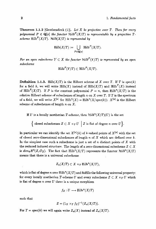
T h e o r e m 1.1.2 [Grothendieck (1)]. Let X be projective over T. Then for every
polynomial P E Q[x] the functor 7-lilbP(X/T) is representable by a projective T- scheme HilbP(X/T). 7-lilb(X/T) is represented by
Hilb(X/T) := U HilbP(X/T)" PEQ[x]
For an open subscheme Y C X the functor 7"lilbP(Y/T) is represented by an open subscheme
HilDP(Y/T) C HilDP(X/T).
D e f i n i t i o n 1.1.3. Hilb(X/T) is the Hilbert scheme of X over T. If T is spec(k)
for a field k, we will write Hilb(X) instead of Hilb(X/T) and Hi lbP(x ) instead
of HilbP(X/T). If P is the constant polynomial P = n, then Hilbn(X/T) is the
relative Hilbert scheme of subschemes of length n on X over T. If T is the spectrum
of a field, we will write X In] for Hilbn(X) = Hilbn(X/spec(k)). X["] is the Hilbert
scheme of subschemes of length n on X.
If U is a locally noetherian T-scheme, then Tlilbn(X/T)(U) is the set
closed subschemes Z C X XT U Z is flat of degree n over U}.
In particular we can identify the set X['q(k) of k-valued points of X In] with the set
of closed zero-dimensional subschemes of length n of X which are defined over k.
In the simplest case such a subscheme is just a set of n distinct points of X with
the reduced induced structure. The length of a zero-dimensional subscheme Z C X
is dim~H~ Oz). The fact that Hilbn(X/T) represents the funetor 7-lilbn(X/T) means that there is a universal subscheme
Zn(X/T) C X XT Hilbn(X/T),
which is fiat of degree n over Hilbn(X/T) and fulfills the following universal property:
for every locally noetherian T-scheme U and every subscheme Z C X XT U which
is flat of degree n over U there is a unique morphism
f z : U -----* Hilbn(X/T)
such that
Z = ( l x XT f z ) - I (Z . (X /T ) ) .
For T = spee(k) we will again write Z,,(X) instead of Zn(X/T).

1.1. The ttilbert scheme 3
R e m a r k 1.1.4. It is easy to see from the definitions that Zn(X/T) represents the
functor Zn(X/T) from the category of locally noetherian schemes to the category
of sets which is given by
Z,(X/T)(U) { (Z, a) Z closed subschemes of X x T U, ]
flat of degree n over U, / a : U ----+ Z a section of the projection Z * U
Zn(X/T)(r : Z , (X/T)(U) ----+ Z,(X/T)(V);
( z , ~) , , ( z • v v , ~0r
(U, V locally noetherian schemes ff : V ~ U).
For the rest of section 1.1 let X be a smooth projective variety over the field
k.
De f in i t i on 1.1.5. Let G(n) be the symmetric group in n letters acting on X n by permuting the factors. The geometric quotient X (n) := X"/G(n) exists and is
called the n-fold symmetric power of X. Let
~ . : X n __ , X(")
be the quotient map.
X (n) parametrizes effective zero-cycles of degree n on X, i.e. formal linear
combinations ~ ni[xi] of points xi in X with coefficients ni E *W fulfilling ~ ni = n. X (~) has a natural stratification into locally closed subschemes:
De f in i t i on 1.1.6. Let u = ( n l , . . . , nr) be a parti t ion of n. Let
i n l := { ( X l , . . . , X n , ) Xl ~.X2 . . . . . Xni} c X n'
be the diagonal and r r
x : := I I c I I x " ' = x " i = 1 i = 1
Then we set
x~ (") := + . ( x"~ )
and
:= x!")\ U
Here # > u means that # is a coarser part i t ion then u.

4 1. Fundamental facts
The geometric points of X (n) are
x ( n ) ( - k ) m ( Z n i [ x i ] E x ( n ) ( - k ) the points xi axe pairwise distinct }.
The X (~) form a stratification of X (n) into locally closed subschemes, i.e they axe
locally closed subschemes, and every point of X (n) lies in a unique X (~). The
relation between X [~] and X (n) is given by:
T h e o r e m 1.1.7 [Mumford-Fogarty (1) 5.4]. There is a canonical morphism (the Hilbert Chow morphism)
y["] X(n), CO n : ~ L r e d )
which as a map of points is given by
z Z xEX
~r y[n] . So the above stratification of X (n) induces a stratification . . . . red"
Defin i t ion 1.1.8. For every partition u of n let
X In] : : conl (x(n) ) .
Then the X[~ n] form a stratification of y[n] into locally closed subschemes. . L r e d
For u = ( n l , . . . , nr) the geometric points of X In] are just the unions of sub-
schemes Z1 , . . . , Zr, where each Zi is a subscheme of length ni of X concentrated in
a point xi and the xi are distinct.

1.2. The Weil conjectures
We will use the Weil conjectures to compute the Betti numbers of Hilbert
schemes. They have been used before to compute Betti numbers of algebraic vari-
eties, at least since in [Harder-Narasimhan (1)] they were applied for moduli spaces
of vector bundles on smooth curves.
Let X be a projective scheme over a finite field Fq , let J~'q be an algebraic
closure of s and X := X x Fq ~'q" The geometric Frobenius
Fx : X - - + X
is the morphism of X to itself which as a map of points is the identity and the map
a ~-~ a q on the structure sheaf Ox. The geometric Frobenius of X over Fq is
Fq := Fx x l~q.
The action of Fq on the geometric points X ( F q ) is the inverse of the action of the
Frobenius of Fq. As this is a topological generator of the Galois group Gal(F~, Fq) ,
a point x E X ( F r is defined over Fq , if and only if x = Fq(x). For a prime I which
does not divide q let Hi(X, Q~) be the i th l-adic cohomology group of X and
bi(--Z) := dimq,(Hi(-x, Ql)),
p(Y, z) := b,(X)z
e(X) :=
b~(X) is independent of I. We will denote the action of Fq* on H~(X , QI ) by
F~]Hr(~,Q~). The zeta-function of X over Fq is the power series
Zq(X't) := exp (n~>o 'X(Fq" )'tn /
Here IMI denotes the number of elements in a finite set M.
Let X be a smooth projective variety over the complex numbers C. Then X
is already defined over a finitely generated extension ring R of 2~, i.e. there is a
variety XR defined over R such that Xn • n C = X. For every prime ideal p of R
let Xp := Xn • n R/p. There is a nonempty open subset U C spec(R) such that
Xp is smooth for all p E U, and the l-adic Betti-numbers of Xp coincide with those
of X for all primes l different from the characteristic of Alp (cf. [Kirwan (1) 15.],
[Bialynicki-Birula, Sommese (1) 2.]. If m C R is a maximal ideal lying in U for
which R / m is a finite field ~'q of characteristic p r l, we call Xm a good reduction of X modulo q.

6 1. Fundamental facts
T h e o r e m 1.2.1. (Well conjectures [Deligne (1)], c]. [Milne (1)1 , [Mazur (1)1)
(1) z ~ ( x , t ) is a rational ]unction
2d
Zq(X, t) = ~ I Q~(X, t) (-1Y+' r ~ 0
with Q~(X, t) = det(1 - tFr [Hr(~,q,))-
(2) Q~(X,t) e 2g[t].
(3) The eigenvalues ai,r of Fq*[Hr(~-,q,) have the absolute value tail[ = at~2 with respect to any embedding into the complex numbers.
(4) Zq(X, 1/qdt) = 4-qe(-x)/2t~(~) Zq(X, t).
(5) If X is a good reduction of a smooth projective variety Y over C, then we have
bi(Y) = bi(X) = deg(Qi(X, t)).
R e m a r k 1.2.2. Let F(t, s l , . . . ,sin) e Q[t, s l , . . . ,sin] be a polynomial. Let X and
S be smooth projective varieties over F q such that
IX(Fq.)l = F(q", [S(Fq,)[,..., I S ( F q - , - ) t )
holds for all n E ~N'. Then we have
p(X, - z ) = F(z 2, p(-S, - z ) , . . . , p(-S, _zm)).
If X and S are good reductions of smooth varieties Y and U over C, we have:
p(V , - z ) = F(z2 ,p (U, - z ) , . . . ,p(V,-zm)) .
P r o o f i Let a l , . . . , a s be pairwise distinct complex numbers and h i , . . . , hs E Q.
We put
Then we have $
z ( ( a , , h,),) = I I ( 1 - a ,) -h, i = 1

1.2. The Well conjectures 7
So we can read off the set of pairs {(al ,h l ) , . . . (as ,hs)} from the function
Z((ai,hi)i). For each c �9 C let r(c) := 21ogq(Icl). By theorem 1.2.1 we have:
for a smooth projective variety W over F q there are distinct complex numbers
(ii)~=l �9 C and integers (li)~=l �9 2g such that
t
IW(Fq-)l = ~ li!~ i=1
for all n E/V. Furthermore we have r ( t i ) E ~_>0 and
(-1)%(w)= ~ l, ~(~)=k
for all k E 2~_>o. Let i l l , . . . , i t E C, l l , . . . ,lt E 2~ be the corresponding numbers
for S. Then we have for all n E ZW:
t t
F [ n K"~l~n "', mn) IX(Fc)I = kq ,~...~ iPi ," E l i t i �9 " i=1 i = 1
Let ~ 5 1 , . . . , ~ r be the distinct complex numbers which appear as monomials in q and
the 7i in
(• • I m F q, l i f l i , . . . , i!i �9 " i=1 i = 1
Then there are rational numbers h i , . . . , n~ such that
IX(Fqo)l = ~ n,e~ i = 1
for all n E SV and
(-i)%(X)= ~ ni r(~j )=k
for all k E 2g>0. We see from the definitions that ~r(6~)=k nj is the coefficient of z k in F(za ,p(S , - z ) , . . . ,p(S,--zm)). [3
We finish by showing how to compute the number of points of the symmetric
power X (n) for a variety X over Fq . The geometric Frobenius F := Fq acts on X(n)('Fq) by
F ( E n i [ x i ] ) = E n i [ F ( x i ) ] ,
axtd X ( " ) ( F q ) is the set of effective zero-cycles of degree n on X which are invariant
under the action of F .

8 1. Fundamental facts
D e f i n i t i o n 1 .2 .3 . A zero-cycle of the form r
E[Fi(x)] with x �9 X(~b-'q. ) \ U Z(ZWq ~ ) i = 0 j[r
is called a primitive zero-cycle of degree r on X over Z~'q. The set of primitive
zero-cycles of degree r on X over hrq will be denoted by Pr(X, ~'q).
Ix(")(Fq)lt" n>O
R e m a r k 1.2.4.
(1) Each element ( E X ('0 (~'q) has a unique representation as a linear combination
of distinct primitive zero-cycles over F q with positive integer coefficients.
(2) IX(Fq.)l = y ] r . IP~(X, Fq)I tin
(3) Zq(X,t) = ~ Ix(")(z~q)l~", n > O
i.e. Zq(X, t) is the generating function for the numbers of effective zero-cycles
of X over s
r P r o o f : (1) Let ( = ~ i=x ni[xi] E X(n)(lFq), where z l , . . . , xr are distinct elements
of X(-~q). For all j let {j := En,kj[xi] �9 X(")(Fq). Then we have ( = y] j (j , and
it suffices to prove the result for the {j. So we can assume that ( is of the form
( = ~i~=l [xi] with pairwise distinct xi E X(-~q). As we have F({) = {, there is a
pe rmu ta t i ona of { 1 , . . . , r } with F(zi) = x~(i) for alli. Let M s , . . . , M s C { 1 , . . . , r }
be the distinct orbits under the action of g. Then we set
r/j := E [xi] iEMj
for j = 1 , . . . s . Then ~ = ~j=ls r/j is the unique representation o f ~ as a sum of
primitive zero-cycles.
(2) follows immediately from the definitions. From (1) we have
= I I ( 1 -- tr)-lP.(X,F,)l T_>I
= Zq(X, t).
So (3) holds. []

1.3. T h e p u n c t u a l H i l b e r t s c h e m e
Let R := k[[x l , . . . , Xd]] be the field of formal power series in d variables over a
field k. Let m = (Xl . . . . ,Xd) be the maximal ideal of R.
D e f i n i t i o n 1.3.1 . Let I C R be an ideal of colength n. The Hilbert function T ( I )
of I is the sequence T( I ) = (ti(I))i>o of non-negat ive integers given by
ti = d i m k ( m l / ( I A m i + mi+l ) ) .
If T = (ti)i>_o is a sequence of non-negat ive integers, of which only finitely many do
not vanish, we put IT I = ~2 ti. The initial degree do of T is the smallest i such tha t ti < (d+i-1) .
Let Ri := m i / r n i+1 and Ii := ( m I Cl [ ) / ( m i+1 (-I I). Then Ri is the space of
forms of degree i in R and Ii the space of init ial forms of I (i.e. the forms of minimal
degree among elements of I ) of degree i, and we have:
t i ( I ) = d imk(Ri / I i ) .
Let I C R be an ideal of colength n and T = (ti)i>_o the Hilbert function of I .
L e m m a 1.3 .2 .
(1) dim(mJ / I N m / ) = E ti
i>_j
holds for all j > O. In particular we have IT] = n.
(2) m".
P r o o f : Let Z := R / I , and Zi the image of m i under the projec t ion R ~ Z. Then we have
N Zi = 0 . i>0
As Z is finite dimensional , there exists an i0 with Zio = O. For such an i0 we have
I D m i~ There is an i somorphism
Zj = m J / ( m j N I) ~- ~ i ~ ~v i=j -~t/
of k-vector spaces, and Ri / I i = 0 holds for i > i0. If we choose io to be minimal ,
then Ri / I i 7 s 0 holds for i < io. So we get (1). If t j = 0 for some j , then I D m j.
Thus (2) fo l lows f rom Irl = n.

10 1. Fundamental fact~
In a similar way one can prove: Let X be a smooth projective variety over an
algebraically closed field k. Let x E X be a point and Z C X a subscheme of length
n with supp(Z) = x. Let Iz , , be the stalk of the ideal of Z at X. Then we have
n Iz , , D m x , ~.
(Just replace R by Ox,~ in the proof above.)
R e m a r k 1.3.3. As every ideal of colength n in R contains m n, we can regard it
as an ideal in R / m ~. Thus the Hilbert scheme Hi lbn(R/m n) also parametrizes the
ideals of colength n in R. We also see that the reduced schemes (Hi lb~(R/mk) )~d
are naturally isomorphic for k _> n. We will therefore denote these schemes also
by Hilbn(R)~d . Hilb~(R)~d is the closed subscheme with the reduced induced
structure of the Grassmannian Grass(n, R / m ~) of n dimensional quotients of R / m ~
whose geometric points are the ideals of colength n of k [ [x l , . . . , Xd]]/m ~.
Using the Hilbert function we get a stratification of Hilbn(R)red .
Def in i t i on 1.3.4. Let T = (ti)i>_o be a sequence of non-negative integers with
ITI = n. Let Z T C Hilbn(R)red be the locally closed subseheme (with the reduced
induced structure) parametrizing ideals I C R with Hilbert function T. Let GT C
ZT be the closed subscheme (with the reduced induced structure) parametrizing
homogeneous ideals I C R with Hilbert function T. Let
PT : ZT ) GT
be the morphism which maps an ideal I to the associated homogeneous ideal (i.e.
the ideal generated by the initial forms of elements of I). The embedding GT C ZT is a natural section of PT.
In the case d = 2 i.e. R = k[[x, y]] many results about these varieties have been
obtained in [Iarrobino (2), (4)].
De f in i t i on 1.3.5. The jumping index (ei)i>o of (ti)i>_o is given by ei = max(t i -1 -
ti, 0).
T h e o r e m 1.3.6. [Iarrobino (4), prop. 1.6, thm. 2.11, thin. 2.12, thm. 3.13]
(1) ZT are GT non-empty if and only if to = 1 and ti <_ ti-1 for all i > do (here again do is the initial degree of T).

1.3. The punctual Hilbert scheme 11
(2) GT and ZT are smooth, GT is projective of dimension
dim(GT) = ~ ( e i + 1)e~+1.
(3) PT : ZT ~ GT is a locally trivial fibre bundle in the Zariski topology, whose
fibre is an aj~ne space A n(T) of dimension
n(T) = n - E (ei + 1)(ej+l + ej /2) . j>_do

2. C o m p u t a t i o n o f t h e B e t t i n u m b e r s o f H i l b e r t s c h e m e s
The second chapter is devoted to computing the Betti numbers of Hitbert
schemes of points. The main tool we want to use are the Well conjectures. In
section 2.1 we will s tudy the structure of the closed subscheme X ['] of X["] which (-) parametrizes subschemes of length n on X concentrated in a variable point of X. We
will show that (X(n))r,d is a locally trivial fibre bundle over X in the Zariski topology
with fibre Hi lb"(k[[xl , . . . xd]]). We will then also gtobalize the stratification of
Hilbr'(k[[xl . . . , Xd]]) from section 1.3 to a stratification of X ["] Some of the strata , (~,). parametrize higher order data of smooth m-dimensional subvarieties Y C X for
m _< d. In chapter 3 we will study natural smooth compactifications of these strata.
In section 2.2 we consider the punctual Hilbert schemes Hilbn(k[[x, y]]). We
give a cell decomposition of the strata and so determine their Betti numbers. I have
published most of the results of this section in a different form in [G6ttsche (3)].
They have afterwards been used in [Iarrobino-Yameogo (1)] to s tudy the structure
of the cohomology ring of the GT. We also recall the results of [Ellingsrud-Stromme
(1),(2)] on a cell decomposition of Hilb"(k[[x, y]]) and p~n].
In section 2.3 we compute the Betti numbers of S ['~1 for an arbitrary smooth
projective surface S using the Weil conjectures. This section gives a simplified
version of my diplom paper [G6ttsche (1),(2)]. The auxiliary results that we prove
here will be used several times in the rest of the chapter. We also formulate a
conjecture for the Hodge numbers of the S In]. In a joint work with Wolfgang Soergel
[G6ttsche-Soergel (1)] it has in the meantime been proved. Independently Cheah
[Cheah (1)] has recently obtained a proof using a different method. One can see
that the Euler numbers of the S In] can be expressed in terms of modular forms. By
the conjecture on the Hodge numbers this is also true for the signatures.
In section 2.4 we compute the Betti numbers of higher order Kummer varieties
KA,,. These varieties have been defined in [Beauville (1)] as new examples of Calabi-
Yau manifolds. While for a general surface S only the symmetric group G(n) in
n letters acts on S n in a natural way by commuting the factors, there is also a
natural action of G(n + 1) on An. KAn can be seen as a natural desingularisation of
the quotient An/G(n + 1). To determine the Betti numbers we again use the Well
conjectures. One can easily see from the formulas that the Euler numbers of the
K A, can be expressed in terms of modular forms. It was shown in [Hirzebruch-HSfer
(1)] that the formula for the Euler numbers of the S In] from section 2.3 coincides
with the orbifold Euler number e(S", G(n)) of the action of G(n). We show that
the Euler number of KA,, coincides with the orbifold Euler number e(A'*, G(n + 1)).
As in section 2.3 we formulate a conjecture for the Hodge numbers. From this we
also get an expression for the signatures of the KAn in terms of modular forms.
In section 2.5 we study varieties of triangles. As mentioned above X [3] is
smooth for an arbitrary smooth projective variety X. So we can use the Weil

2. Betti numbers of Hilbert schemes 13
conjectures to compute its Betti numbers. We can view X [3] as a variety of unordered
triangles on X. From X [3] we can construct several other varieties of triangles on ~ 3
X. The variety Hilb (X) of triangles on X with a marked side has been used in
[Elencwajg-Le Barz (3)] in the case of Z = P2 to compute the Chow ring of p~3],
and the variety H 3 ( X ) of complete triangles on X has been studied in detail in
[Roberts-Speiser (1),(2),(3)], [Collino-Fulton (1)] for X = P2. For general X it has
been constructed in [Le Barz (10)]. There is also a new functorial construction by
Keel [Keel (1)]. We will construct two additional varieties of triangles. We show
that they are smooth and s tudy maps and relations among the triangle varieties.
Then we use the Well conjectures to compute their Betti numbers.

14
2.1. T h e l o c a l s t r u c t u r e o f X In] (,0
Let k be a (not necessarily algebraical ly closed) field and X a smooth quasipro-
jective variety of dimension d over k. In this section we s tudy the s t ructure of the
s t r a tum (X(n))~d which parametr izes subschemes of X which are concentra ted in
a (variable) point in X.
D e f i n i t i o n 2 .1 .1 . Let X be a smooth project ive variety over a field k. Let A C
X x X be the diagonal a n d Z A / x x x its ideal. Let A n C X x X be the closed
subscheme which is defined by Z~x/x xX" Let
pl,P2 : X • X ~ X
be the project ions and /51,/52 the restr ict ions to A n. The (n - 1) th jet-bundle
Jn-1 (X) of X is the vector bundle associated to the locally free sheaf
J , _ , ( X ) := (p2) , (O~o)
on X. More general ly let Z ~ V A . be the ideal sheaf of A i in A n and J / _ a ( X ) be
the vector bundle associated to
J n ' _ , ( X ) := (p2),(ZA,/A.)
for all i < n - 1.
We see tha t the fibre Jn_l(X)(x) of Jn-a (X) over a point x e X can be identi-
fied in a na tu ra l way with Ox,~/mnx,x and similar ly Jn_l(X)(x) with m x , J m x , x . ~ n
We have
Symi(T; ).
H i l b n ( A n / X ) is a locally closed subscheme of
Hi lbn(X • X / X ) = Hi lbn(X) ,
and there is a na tu ra l morphism
r : H i l b ~ ( A n / x ) ~ X.
L e m m a 2.1 .2 . Hilb'~(An/X)r~d YX In] ~ : ~ (n))r~d as subschemes of X In] and 7r :
(X['q (n))~d ---* X is given by mapping a subscheme of length n which concentrated is
in a point to this point.

2.1. The local structure of X ['q 15 (n)
P r o o f i Let k be an algebraic closure of k a n d X - := X x k k . Let Z C X be a
subscheme of length n of X concentrated in a point, Iz its ideal in the local ring
Ox,~ and m x , , the maximal ideal of Ox,~. Then we have Iz D m ~ (cf. 1.3.2). X,x
So we see that Hilb"(An/X)red and ~X [ 'q ' t (n))r~d are closed subschemes of X [~] with
the reduced induced structure, which have the same geometric points. Thus they
are equal. The assertion on 7r follows directly from the definitions. D
Let Grass(n, Jn-l(X)) be the Grassmannian bundle of n-dimensional quo-
tients of Jn -~(X) let and # : Grass(n, J n - l ( X ) ) ~ X be the projection.
L e m m a 2.1.3. There is a closed embedding
o v e r X .
P r o o f : Let
~ : Hilb"(A"/X)r~a , Grass(n, Jn-1 (X))
Z,(A"/X) C A" x x H i l b " ( A " / X )
be the universal family (cf. 1.1.3) and let
t52 : A" x x H i l b " ( A n / X ) ~ Hi lbn(An/X)
be the projection. Then we have
(#2),(Oa.x,:Hilb.(a./x)) -- ~r*(Jn-l(X)) .
As Zn(An/X) is flat of degree n over Hi lb~(A~/X) , ([~2),(Oz.(A./x)) is a locally
free quotient of rank n of 7r*(d~_a(X)). Thus it defines a morphism
i : Hi lbn(An/X) , Grass(n, dn-l(X)).
So we also get a morphsim
3: Hi lb"(A"/X)red ~ Grass(n, Jn-l(X)).
Let T be the tautological subbundle of corank n of fr*(dn_l(X)). We abreviate
Grass(n, Jn-l(X)) by Y. r is in a natural way an Oy-algebra. Let Q
be the quotient of ~c*(ffn_l(X)) by the subalgebra generated by T. Q is a coherent
sheaf on Y. For all x in Y let
q(x) : = dimk(G • x Oy, . /my, .)

16 2. Betti numbers of Hilbert schemes
be the rank of Q at x. From the definitions we see that q(x) <_ n holds for all x �9 Y.
Let H C Y be the closed subscheme with the reduced induced structure, for whose
points q(x) = n holds. Then we see
~(Si lbn(A~/X)r~d) C H.
Let ~" : H ~ X be the restriction of the projection. Let A n := A n x x H and
152 : h " ~ H be the projection. Then we have (/32),(Os = #* ( Jn -~ (X) ) . As
/~2 is an homeomorphism, we can view Q as a quotient of OA- i.e. as the structure
sheaf of a subseheme Z of /~n , which is flat of degree n over H. This defines a
morphism
j : H ~ Hilbn(An/X)~r
From the definitions it is clear that j is the inverse of i. []
For the rest of the section we want to assume in addit ion that there are an
open cover (Ui)i of X and local parameters on each of the Ui defined over k. Let
R := k[[x~, . . . , xd]], m := ( z ~ , . . . , xd) be the maximal ideal of R and let Hilb'~(R)~d
be the Hilbert scheme parametrizing ideals of colength n in R / m ~ (cf. 1.3.3).
' X In] ~ X i~ a locally trivial fibre bundle in the Zari~ki L e m m a 2.1.4. 7r : ~ ( n ) ) r e d ------+
topology with fibre Hilbn(R)~d .
P r o o f : Let U C X be an open subset and Yl , . . . Yd local parameters on U. For
each g �9 k[ [x l , . . . ,Xd]]/m" let
Y : : g((f2),(~7(yl) - /5~(yl) ) , . . . , (P2),(PT(yd) -/5~(yd))) �9 r(Jn-~(U)).
We see that the ~" are a basis of Jn-l(U) in each fibre. Thus there is an isomorphism
R / m n | Ou ~- J n - l ( U ) and so also an isomorphism
e n : U x G r a s s ( n , R / m n) ~ Grass(n, J,~_, (U)).
We see that the image of
U x Hilb"(n)r~d C U x G r a s s ( n , n / m n)
under en is ~'-I(U) ~ { t u [ n ] , , : �9 n = t< (n))red)" So the restriction of en to U x Hs (R)~d is
H" n ,Ub ] an isomorphism r : U x Jb ( R ) r e d ~ < (n)]re d. []
We can globalize the stratification of Hilbn(R)~,d to a stratification of (Xtn],
( n ) ) r ed"

2.1. The local structure ~ Y[~] 17 ~J -~(~)
D e f i n i t i o n 2.1.5. For i = 1 , . . . , n - 1 let
~)i: J / _ l ( X ) ~ J~(X) ~- Symi (T*X)
be the canonical map. Let T = ( to , . . . , t ~ - l ) be a sequence of non-negative inte-
gers. Let ~ : Grass(n, J,~-i (X)) , X be the projection as above. Let T be the
tautological subbundle of ~r*(Jn-l(X)). For all i let
Q, := ~*( J~_I(X))/(T n #*( Ji_l(X)) + ~ * ( J / + I ( x ) ) ) .
Let WT C Grass(n, Jn-~ (X)) be the locally closed subscheme over which the rank
of Qi is ti for all i. Let
[~] zT (x ) = ~-I(wT) c (x(~))~d
with the reduced induced structure. Let rrT : ZT(X) --~ X be the projection.
Qilzr(x) is a quotient bundle of rank ti of ~@(Symi(T~()).
Let Ti be the tautological subbundle on Grass(ti, Symi(T~) . Let
7r1: H G r a s s ( t i , Symi(r~() ----+ X i
be the projection and
V~(X) c H aTass(tl, Sym'(T~) i
the closed subvariety over which
T~. ~;(T~) r T~+I
holds for all i. Here T1- 7r~'(T~) denotes the image of 7'1 | ~r~(T~) by the natura l
vector bundle morph ism
7r~(Symi(T~) | T~) ~ Tr~(Symi+a(T~:)).
Let
p T ( x ) : z v ( x ) , c v ( x )
be the morphism defined by the bundles Qi]ZT(X).
Analogously to the proof of l emma 2.1.4 we can easily see:
R e m a r k 2 . 1 . 6 .

18 2. Betti numbers of Hilbert ~cherne~
(1) ZT(X) and GT(X) are locally tr ivial fibre bundles over X with fibres ZT and
GT respectively.
(2) W i t h respect to local t r ivial isat ions
ZT(U) ~ U X ZT,
GT(U) ~- U X GT
over an open subset U C X we have pT(U) ~- 1u • PT.
R e m a r k 2 . 1 . 7 .
all s �9 JTV
We can see from the definitions tha t for all l _< d = dim(X) and
))( ' . G(1, I , ( t+ I ) ..... (t-I-;-, X) = Grass(l, Tfc ).
with fibre A r over Z(1,/,(,+l ~ , . - . ........('+;-1]](X) is a locally tr ivial fibre bundle
G(1,t,(,+l ) ..... ( ,+ :_ , ) ) (X) . Here r : - ( d - l ) ( ( t l s ) - l - 1 ) .
P r o o f : By remark 2.1.6 we have to prove this only for
Hi lb( '+ ' ) (R) . a(,,, ,( ,+,) ..... ( ,+:_,)),Z(, , , ,( ,1,) ..... (,+;_,)) c
The assert ion forG(,,t,(,+,~,,, ..... (,+:_,)) is obvious. Now let Z � 9 Z(,,t,(,+, ~ , , , ( '+7 ' ) )
and let Iz be the ideal of Z. Then there are y t + l , . . . , yd in R such that I z is given by Iz = (Yt+l, . . . ,Ya) + m ~+1. The init ial forms ui of the yi all have degree 1 and
are l inearly independent . We can assume tha t x 1, �9 �9 �9 xl, ul+ 1, � 9 u d are l inearly
independent . We can modify the Yi to be of the form
Yi : Ui + f i (Xl , . . . ,X l ) .
The f i ( x l , . . . , xt) can be a rb i t r a ry polynomials in x l , . . . , xt of degrees < s, whose
in i t i a l forms hasve degree > 2. Thus the result follows. []
R e m a r k 2 .1 .8 . Of par t i cu la r impor tance is the s t r a t um Z(1 ..... 1)(X) C X ['q It (~)-
is an open subvariety of X ['q It is however in general not dense in X ["] if d > 3 (n)- (n) - a n d if n is large. By the definitions it parametr izes subschemes of X which are
concent ra ted in a point z and lie on (the germ of) a smooth curve through z. We
Y['q is a will therefore also wri te X I'q ins tead of Z(1 ..... 1)(X). By remark 2.1.7 ~'(n),r (n),c locally tr ivial A(d -O(n-2 ) -bund le over P(Tx) .

19
2.2. A cell d e c o m p o s t i o n of p~n], Hilbn(R), Z T ' GT
Let k be an algebraically closed field. In this section we review the methods of [Ellingsrud-Str0mme(1)] for the determination of a cell decomposition of p~n] and
modify them in order get a cell decomposition and thus (for k = C) the homology
of the strata Z T and GT of Hilbn(k[[x, y]]). Let R := k[[x, y]]. Let Hilbn(A 2, 0) be
the closed subscheme with the induced reduced structure of (A2) In] parametrizing
subschemes with support {0}. By lemma 2.1.4 we have
Hilbn(A 2, 0) ~ Hilb~(R)r~d .
In [Ellingsrud-Stromme (1)] the homology groups of p~n] A~, q and Hilbn(A 2, 0) are
computed by constructing cell decompositions. We review some of the results and
definitions on such cell decompositions. For a complex variety X let H . ( X ) be the
Borel-Moore homology of Z with 2g coefficients. For each i let bi(X) = rk (Hi (X) )
be the i th Betti number and e(X) = ~-~(-1)%i(Z) the Euler number. Let A m ( X )
be the mth Chow group of X and cl : A . ( X ) , H . ( X ) the cycle map (cf. [Fulton
(1), 19.1]). For X smooth projective of dimension d we put A m ( x ) = Ad-m(X) .
Defini t ion 2.2.1. Let X be a scheme over a field k. A cell decomposition of X is a filtration
X = X n D Xn--1 D . . . DXo D X - 1 = 0
such that Xi \ Xi-1 is a disjoint union of schemes Ui,j isomorphic to affine spaces A n~,j for all i = 0 , . . . , n. We call the Ui,j the cells of the decomposition.
P r o p o s i t i o n 2.2.2. [Fulton (1) Ex. 19.1.11] Let X be a scheme over C with a cell
decomposition. Then
(1) H2i+l(X) = 0 for all i.
(2) H2i(X) is the free abelian group generated by the homology classes of the clo-
sures of the i-dimensional cells.
(3) The cycle map el: A . ( X ) ~ g . ( x ) is an isomorphism.
Ellingsrud and Str0mme have constructed the cell decomposition of p~n] using the following results of [Bialynicki-Sirula (1),(2)]. Let Z be a smooth projective
variety over k with an action of the multiplicative group Gin. We will denote this
action by " . ' . Let x E X be a fixed point of this action. Let T+x,z C Tx,~ be the linear subspace on which all the weights of the induced action of (~,, are positive.
T h e o r e m 2.2.3. [Bialynicki-Birula (1),(2)] Let X be a smooth projective variety
over an algebraically closed field k with an action of Gm. Assume that the set of

20 2. The Bett i numbers of Hilbert schemes
fixed points is the finite se t {Xl, . . . , X m ) . For all i = 1 , . . . , m let
X i : = { x e X I l i m t . x = xi}. t~O
Then we have:
(1) X has a cell decomposition, whose cells are the Xi .
(2) T x , , x , : T + X,xi "
For non-negative integers n k l we denote by p(n) the number of part i t ions of
n and by p(n, l) the number of part i t ions of n into l parts. This number coincides
with the number of part i t ions of n - 1 into numbers smaller or equal to I.
The main result of [Ellingsrud-Str0mme (1)] is:
T h e o r e m 2.2.4. [Ellingsrud-Str0mme (1)]
(1) For X = p~n], X = A~ n] and X = Hilb'~(A 2, 0) the following holds: X has a
cell decomposition. In particular i l k = C the cycle map cl : A , ( X ) ~ H , ( X )
is an isomorphism, H2i+I (X) = O, and the H2i (X) are free abelean groups.
I f k = C the Betti numbers are
(2) b21(P~ hI) = ~ ~ p(no,no - ko)p(nl)p(n2,k2 - n2), noq-nl q-n2=n ko+k2=l-nl
(3) b2,(n~ nl) = ; ( ~ , l - ~),
b2t(Hilbn(A 2, 0)) = p(n, n - l).
We will briefly review the ideas of the proof in [Ell ingsrud-Strcmme (1)]. Let
To, T1, T2 be a system of homogeneous coordinates on P2- Let G C Sl(3, k) be the
maximal torus consisting of the diagonal matrices. Let A0, A1, A2 be characters of G
such that all the g ~ G can be writ ten as
g = diag(~o(g),Al(g),A2(g)).
G acts on P2 by g �9 T / = Ai(g)Ti. The fixed points of this action are
eo -- (1 ,o ,o) ,
P1 = (o, 1,o),
P2 =(o,o,1).

2.2. A cell decompostion of P~n], Hilbn(R), ZT, a T 21
The action of G on P2 induces an action of G on p~n], as G acts on the ideals in
k[To, T1, T2]. Z E p~n] is a fixed point if and only if the corresponding homogeneous
ideal I z C k[To,T1,T2] is generated by monomials. So the action on P~'q has only
finitely many fixed points.
Let X be a smooth projective variety over k with an action of a torus H which
has only finitely many fixed points. A one-parameter subgroup �9 : Gm ~ H of H
which does not lie in a finite set of given hyperplanes in the lattice of one-parameter
groups of H will have the same fixed points as H. In future we call such a one-
paramete r group "general". Thus the induced action of a general one-parameter
group q~ : G m ----* G has only finitely many fixed points on P~'q.
Let �9 : Gm -----+ G be a general one-parameter group of the form @(t) =
d i a g ( t W ~ with w0 < wl < w2 and w0 + wl + w2 = 0. Let F0 := {P0},
L C P2 the line T2 = 0, /;'1 := L \ P 0 e F2 := P 2 k L . Then ~5 induces the cell decomposit ion of P2 into F0, F1, F2. Ellingsrud and S t rcmme apply theorem 2.2.3
to the induced Gm-act ion on P~] . We will modify their arguments in order to
obtain a cell decomposit ion of the s t ra ta Z T of Hilbn(R).
We denote by "." the action of Gm on p~nl induced by q~. As it has only
finitely many fixed points, it gives a cell decomposit ion of p~n]. Hi lbn(R)~d =
Hilbn(A 2, 0) C P~] is the subvariety parametr iz ing subschemes Z of colength n
with support s u p p ( Z ) = {P0}. If Z e P~'q has support {P0}, then
suppQin~( t . Z ) ) -- t--.olim( t . supp( Z ) ) = {P0}.
If s u p p ( Z ) 7~ {P0}, then we have
z)) = upp(Z)) r (P0}.
So
Z e Hilbn(A 2, 0) r l im(t �9 Z) �9 Hilbn(A 2, 0).
So by theorem 2.2.3 Hilbn(A 2, 0) is a union of cells of the cell decomposit ion of P~'~]
which belong to fixed points in Hilbn(A2,0). In part icular Hilb'~(A2,0) has a cell
decomposition.
Using the identification := T I lTo ,
y :=T21To,
R := \[Ix, y]]
we have Hilbn(A 2, 0) = Hilbn(R)r~d . We identify the points of Hilbn(R)r~d with the
ideals of colength n in R. The action of Gm on R and thus on Hilb'~(R) is given by
t . x = twl-W~
t " y = tw~-W~

22 2. The Betti numbers of Hilbert schemes
Let I E Hilb"(R) be a fixed point. Then I is an ideal of colength n in R which is
generated by monomials. Following Ellingsrud and Str~mme we put
aj : = rain{1 I xJY I E I }
for every non-negative integer j. Let r be the largest integer with ar > 0. Then
(a0,. �9 �9 at) is a partition of n, and y ,0 x y , l . . . , xr+l are a system of generators of
I. So there is a bijection between the cells of Hilbn(R) and the partitions of n. In
particular the Euler number of Hilbn(R) is p(n).
Let T be the tangent space of Hilb"(A 2) in the point corresponding to I. Let
F be a two-dimensionM torus acting on R by
t . x = ~ ( t ) x ,
t . v = # ( t ) y
(here t e P and A, # are two linearly independent characters of r). We also de-
note by ,~ and # the corresponding elements in the representation ring of F. By
[Grothendieck (1)] there is a F-equivariant isomorphism
T ~- gomn(I , R/I).
Ellingsrud and Strcmme consider the corresponding representation of P on T. They
get:
L e m m a 2.2.5. In the representation ring of F there is the identity
T = aj -1
E E O<_i<j<_r s=ai +t
( )~ i--j--l #al--s--1 _]_ )~j--i #s--al ).
We give a simple proof of this result: The lemma says that T has a basis of
common eigenvectors to F with the eigenvalues as in the above formula. By
E . 2 ( a j - a j + l ) = 2 E a i = 2 n = d i m ( T ) O<i<j<r O < i < r
it is enough to give such linear independent eigenvectors. For f E R let [f] be the
class in R/I . An R-homomorphism r : I ~ R / I is determined by its values on
the xiy a~. They must however be compatible. It is easy to see that necessary and
sufficient conditions for this are
r = [x]r r = [Vo,-1-a,]r

2.2. A cell decompostion of p~n], Hilb~(R), ZT, GT 23
Let 0 < i < j < r and aj > s >_ aj+l. Let
[xJ+l-iy s+a'-a'] i f l _< i, r : I ----+ R / I ; x ly ~ ' ) 0 otherwise.
We can see immediately that the compatibility conditions are fulfilled and r is a common eigenvector of F to the eigenvalue A J - i# ~-a~.
L e t 0 < _ ~ < ~ _ r + l a n d a g - a ~ _ l + a T _ < ~ < a 5. We put
r ~ ~ : I - - ~ R / I ; x ' y ~' , , {~x3+'-~Y a + ~ - ~ ] i f />_~, ' ' otherwise.
r is an eigenvector to the eigenvalue ~)-~#~-a~. The eigenvectors constructed
this way are obviously linearly independent. The result follows by the substi tution
s : = ~ - a ~ +a~
j : = ~ - I
i:----~. []
We now formulate our result on the cell decompositions of ZT and GT in a form
which has been influenced by [Iarrobino-Yameogo (1)]. In particular the formula for
the Betti numbers of GT does not follow immediately from my original formulation. In [Iarrobino-Yameogo (1)] two combinatorical formulas are shown in order to derive
this formula from my original one in [G6ttsche (4)]. Here we will give a direct proof.
D e f i n i t i o n 2.2.6. Let (~ = (a0 , . . . ,aT) be a parti t ion of n. The graph of o~ is the
set
F ( a ) = {(i , / )E2g~_0 i ~ r , l < a i } .
Picturally we can represent F(a) as a set of points, one point in position ( i , j ) for
each ( i , j ) E F(a) . The dual part i t ion & = (~ l , . . - ,~a0) is the partit ion, whose
graph is F(a) with the roles of rows and columns switched. The diagonal sequence
is T ( a ) = ( t o ( a ) , . . . , t l (a)) , where
So it is the sequence of numbers of points on the diagonals of F(a) . Let (u, v) E F(a) .
Then the hook difference h~,v(a) is

24 2. The Betti numbers of Hilbert schemes
I.e. hu,v(a) is the difference of the number of points in F(a) in the same column
above (u, v) and the number of points in the same row to the left of (u, v). So we
have
h~,~(~) = (i~, + v - a~ - u.
For the part i t ion c~ = (6, 3, 2) we get for instance the diagram
for F(c~) and
The hu,v(c~) are given by
& = (3,3,2, 1, 1, 1),
T(c~) = (1,2,3,3, 1, 1).
- 1 0 --1 0 0 --3 --2 - 2 - 2 - 1 O.
T h e o r e m 2.2.7. Let T = (ti)i>_o be a sequence of non-negative integers with
ITI = n. Then we have for X = GT and X = Z r :
(1) X has a ceil decomposition. I f k = C, then cl : A . ( X ) ~ H . ( X ) is an
isomorphism and H . ( X ) is free.
In case k = C we have for the Betti numbers:
(2) b 2 , ( Z r ) = a � 9 i { (u , v ) e V ( a ) l h u , v ( a ) e { o , 1 } } l = n _ i
(3) b2~(Gr )= { a E P ( n ) T ( a ) = T ; I{(u,v) E F ( a ) l h , ~ , ~ ( a ) = l } I = i } .
In particular the Euler numbers are
= = �9 P ( n ) I : T } .
R e m a r k 2.2.8. In [Iarrobino (2),(4)] it has been shown that ZT and GT are non-
empty if and only if to = 1 and ti <<_ ti-1 for a l t i >_ d(T). If T = ( 1 , . . . , 1),

2.2. A cell decompostion of p~n], Hi lb~(R) , ZT; GT 25
then Z T is an A n - 2 - b u n d l e over GT = P1. It is easy to see t h a t to(a) = 1 and
t i(a) <_ t i - l ( a ) for all i >_ d(T(a)) for each p a r t i t i o n a of n. If T = ( 1 , . . . , 1) the
cell decompos i t i on of ZT of t h e o r e m 2.2.7 consists of one cell of d imens ion n - 2
and one of d imens ion n - 1 and tha t of GT of one cell of d imens ion 0 and one cell
of d imens ion 1 as expec ted .
As above let �9 w o W l w 2 (P:Gm-----4G; t ~ d m g ( t ,t , t )
be a genera l o n e - p a r a m e t e r subgroup of G wi th w0 < wl < w~ and w0 + W l + w 2 = 0.
We also requi re the inequa l i ty
n(w l - wo) > (n - l)(w2 - wo).
We consider the induced G m - a c t i o n on Hi lb~(R) . We know a l ready t h a t it gives a
cell decompos i t i on of Hi lbn(R) . Let T = (t i) be a sequence of non -nega t ive in tegers
wi th ITI = n.
L e m m a 2 .2 .9 .
( l ) ZT is it union of cells of the cell decomposition of H i l b ' ( R ) .
(2) PT : ZT ~ GT is equivariant with respect to the Gin-action.
(3) The Gin-action induces a cell decomposition of GT. Its cells are the intersec-
tions of the cells of ZT with GT.
P r o o f : Let I be an ideal in R wi th Hi lber t func t ion T. Let j E f g , s := j + 1 - tj. Let Ij be the space of ini t ia l forms of degree j in I . We pu t
J := l i m t . I . t ~ O
For all i let Ji be the space of in i t ia l forms of degree i in J . Let T I = (t~)j_>0 be the
Hi lber t func t ion of J . Choose f l , �9 �9 �9 f~ E I such tha t the i r ini t ia l forms g l , . �9 �9 g~
are a basis of Ij. By rep lac ing the fi by su i tab le l inear combina t ions we can as sume
tha t the gi are of the fo rm
gi = xl(i)Y j- l( i) ~- E gi ,mxmy j - m
rn>l(i)
wi th gi,m E k and t h a t l(1) > /(2) > . . . > l(s). By the choice of the weights
WO~ Wl ~ W 2 w e get
l im ~ ( t ) - (tt(i)(w~176 f i) = xl(i)y j-l(i). t~O

26 2. The Betti numbers of Hilbert schemes
So the span of the xl(i)y j-l(i) is contained in Jj. So we have
t' i = i + 1 - dim(Ji) <_ tj.
B y IT'I = n we h a v e T = Z ' and thus (1).
(2) follows immediately from the definitions. GT is a smooth projective variety.
I f I E Gr , then we have e 2 ( t ) . I E G:r for a l l t E Gin. S o G m acts on GT w i t h a
finite number of fixed points and we can apply theorem 2.2.3. As the action on GT
is the restriction of that o n ZT, (3) follows. E
To determine the Betti numbers of Z T and GT we have to find out, which of
the Gm-invariant ideals of R lie in ZT and what the dimensions of the corresponding
cells of ZT and GT are. Let a = (a0 . . . . , at) be a partit ion of n and I the ideal of
R generated by yaO, xy~l . . . , xr+l.
L e m m a 2.2.10. For the HiIbert function T(I ) of I we have T(I ) = T(~).
P r o o f i Let T(I) = (ti)i_>0. The monomials xiy I with i + l = j and l > ai form a
basis of the space Ij of homogeneous polynomials of degree j in I . So we have:
t j - - j + l - {(i , /)E2g~_ 0 l i + l = j , l>_ai}
= {( i , j ) e r (~ ) l i + j = l}
= t j ( . ) . []
Let again T be the tangent space of Hilbn(A ~) in the point corresponding to
I .
L e m m a 2.2.11. The dimension of the subspace T + of T on which the weights of
the action are positive is
d im(T + ) = n - {(u,v) e V ( ~ ) ] h u , v ( ~ ) = 0 o r h ~ , v ( a ) = l } .
Proof." We apply lemma 2.2.5 to r -- G and
AI A2
Then we have for every character A~# b of G:
( ) , a ~ b ) ( , ~ ( t ) ) = t o ( , ~ , - ~ , o ) + b ( w , - w o ) .

2.2. A cell decompostion of P~'q, Hilb~(R), ZT, GT 27
By the choice of w0, wl, w2 the action of Gm has a positive weight on ~ # b , if and
only if a + b > 0 or a + b = 0 and b > 0. Let i , j be integers satisfying
O < i < j < r , aj+l < s < aj.
The weight of (,V-3-1 # ~ - ~ - 1 ) o ~ is positive, if and only if i + ai > j + s + 1, and
the weight of ~ j - i~s -a i is positive, if and only if i + ai < j + s. From the definition
we see that /z , is the smallest j satisfying s > a j , so/z, - 1 is the smallest j satisfying
S > a j + l . So we have
E ( { aJ+z <--s<aJ ' } ) dirnT + = aj - aj+ 1 - s E 2~ 0 < j + s - i - ai + 1 < 1 O<_i<_j<_r -- - -
= �9 o < < z}l, []
Let To C T be the tangent space of GT in I . It is easy to see that the
isomorphism T ~ H o m R ( I , R / I ) maps To to the space of degree-preserving homo-
morphisms in Hornn( I , R / I ) . In the representation ring of F the subspace To can
be written as the sum of all terms in the representation of T with a + b = 0. Let
To + C To be the linear subspace on which the weights of the action are positive.
L e m m a 2.2.12.
d i m ( T + ) = {(u,v) C F(a) l hu,v = - 1 } ,
d i m ( T o / T + ) = {(u,v) E F(c~)[ h~,, = 1}.
Proof." Let i , j be integers satisfying
O < i < j < r , aj+l < s < a j .
If i - j - 1 + ai - s - 1 = O, then the weight of ( A i - j - l # a ~ - 8 - , ) o ~ is positive. If
j - i + s - ai = 0, then the weight of (M-i#s-a~)o~5 is negative. So we have
d i m ( T + ) = E I { s E 2 ~ [ a j + l < - s < a j ' i - J + a i - s - 2 = O } l O<_i<j<_r
= E { s E 2 g O < _ s < a i , i + a i - - s - - & , = l } o<_i<r

28 2. The Betti numbers of Hilbert schemes
and
dim(T~ Z I{sc2ZlaJ+, <-s<aj, i + a i - - s - - j = O } l O<i<_j<r
O<:i<r
By putt ing things together that theorem 2.2.7 1s proved.
R e m a r k 2.2.13. We can now easily determine the dimensions of GT and ZT, as
they are both smooth. From lemma 2.2.12 we have:
dim(GT(~)) = { ( u , v ) ~ F(c~) [h,,v(C~)l = 1} .
Let T1 be the tangent space of ZT(~) in I. The isomorphim T ~ Hom•(I, R/I) maps T1 to the space of homomorphisms which preserve or increase the degree. So
T1 can be written as the sum of the terms A,pb in the representation of T for which
a + b > 0. In addition to the terms occuring in T + these are exactly the AJ-iy -a~ w i t h j + s - a i - i = 0 . So we get:
dim( ZT ) = dim(T1)
=dim(T+)+ Z { sE2~ a i + l < - s < a J ' } O<i<_j~r J ~- S -- ai -- i -F 1 ~ 1
=d/re(w+)+
Using theorem 1.3.8 we get for each partit ion c~ of n the combinatorical formulas:
{(?A, Y) ~ r(oL) Ihu,v(O~)] -_ 1} : Z (ci(T(o~)) -~ 1)ei_l_l(T(o:,)) i>_do(T(c~))
{(u, v) E F(a) h, ,v(a) = 0} = Z ei(T(a))(ei(T(a)) + 1)/2. i>_do(T(a))
Here (ei(T(a)))i>o is the jumping index and do(T(a)) the initial degree of T(a) (cf. definitions 1.3.5 and 1.3.1). In [Iarrobino-Yameogo (1)] these two formulas are
proved eombinatorically.

29
2.3. C o m p u t a t i o n of the Bet t i numbers of 5:[~] for a s m o o t h surface 5:
We want to use the Weil conjectures to compute the Bett i numbers of S ["]
for a smooth project ive surface 5: over C. Let X be a smooth project ive variety of
dimension d over a field k. Let R = k [ [ x l , . . . , xd]]. We denote Vn := Hi lb~(R)~a .
We denote by len(Z1) the length of a subscheme Z. For subschemes Z1, Z2 C X we
will wri te Z1 C Zz if Zl is a subscheme of Z2 (the same also if Z1 E Hilb ~ ( R ) ~ d
and Z2 E Hilb~2(R)~d). For
(zl, Zl
(z2,
we write (xl,Z1) C (xz,Z2), if :cl ( n l , . . . , n~) we also write
c (x •
(x •
= z2 and Z 1 C Z2. For a par t i t ion u =
I~,2~,...),
where ai is the number of summands i in u. Let
[a[ := E ai. i
Let P(n) be the set of par t i t ions of n.
U ~ We will assume for the following that there exist a finite open cover ( i)i=l of
X and local parameters on each of the Ui, defined over k.
R e m a r k 2 .3 .1 . There is a sequence of bijections r : X l : l ( k ) ~ (X • V,,)(k),
commut ing with the action of the Galois group Gal(k, k) such tha t
Zl C Z2 "r ~len(Z1)(Zl) C ~)len(Z2)(Z2).
r /U ~[n] Proof: For i = 1 , . . . , s let 7ri : kt i)(n))~ea ----4 Ui be the restr ic t ion of the projec-
tX["] ~ X from lemma 2.1.2. By lemma 2.1.4 there are isomorphisms tion 7r : t (n ) ) red -----+
t /U d n] ~ t : ~,~ i)(n))red ----4 Ui x Vn
over Ui for all n E 2V. Thus we have the required bijeetions r := aS~(k). For all
j = l , . . . , s l e t
w :=vj\Uv i<j
--1 X ['q (k~ there is a unique index i(Z) such tha t W C 7ri(z)(W,(z)). We For e a c h Z E (n) J
put C n ( Z ) : = r The result follows, as all the r are bijective. []

30 2. Betti numbers of Hilbert schemes
Def in i t i on 2.3.2. For any parti t ion v = ( h i , . . . , n~) = (1 ~ , 2~%.. . ) of n let
. x I o , l . ~ H ( x l : l ) o , 2 2 : = ( ~ , , , • • ..... , ) ) c u,,) • x u , ) = i
The symmetric group G(n) acts on X2 via its quotient
a(o~) := a ( , ~ ) x . . . • C(o,~, )
by permuting the factors X [~i] with the same ni. (hi)
L e m m a 2.3.3. There is a natural morphism r : 2 n ~ X In], which induces a bijection
r : X 2 ( k ) / a ( n ) --~ X~l(-~)
commuting with the action of GaI(k, k ).
P r o o f : Let T be a noetherian k-scheme and let (Z~, . . . , Z~) C 22(T). We put
r z~)) := Zl u . . . u z~.
This is obviously flat of degree n over T. ~ is compatible with base change, so it
defines a morphism Cv : 2 ~ - -~ X['q. The induced map r of geometric points
maps )~2(k) to X[~n](k) and is invariant under the action of G(n). So we have a map
r X2(k)/a(~) ~ X~J(~).
The image of Z e X[~n](k) is ~ 2 I ( Z ) = [Z1, . . . ,Z~] , where Z1, . . . ,Z~ are the
connected components of Z and [] the class modulo G(n). []
Def in i t i on 2.3.4. For an extension/~ of k we write
o ~
v(~) := U v,.(~). r=O
Let o be the point corresponding to the empty subscheme i.e. Vo(k) = V0(~) = {o}.
For x E V~(Ic) we put len(x) := r. For a map f : X(k) ~ V(k) we put
Ion(f) := ~ len(f(x)).
~x(~)
Gal(k, k) acts on these maps by
o-(f) := crofoo --1.

2.3. The Betti numbers of S ["1 31
We write f l C f2, if f l (x) C f2(x) for al l x �9 x ( k ) .
L e m m a 2.3.5. There exists a sequence of bijections
commuting with the action of Gal(-k/k) such that
Z1 C Z2 ~ Olen(Z,)(Z1) C Olen(Z2)(Z2).
P r o o f : Let v = ( r t l , . . . ,rtr) be a partit ion of n, and let Z �9 X[n](k) with
~ J ~ - l ( z ) = [ Z l , . . . , Z r ] ,
where len(Zi) = hi. We put
O,(Z) := f : X(k) ---4 V(k);
f p2(O,,(Zi)) if x = (Zi)red, X o if x ~ supp(Z),
where P2 : X x V~
and lemma 2.3.3.
Vn is the projection. The result follows from remark 2.3.1
De f in i t i on 2.3.6. Now let k be a finite field Fq , X a smooth projective variety
over ~'q and F the geometric Frobenius of X over _gTq. Let
P(X,~'q) = U P~(X, Fq) r>0
be the set of primitive zero cycles of X over _~q (cf. 1.2.3). A map g : P(X, Fq) V(/Fq) will be called admissible, if g(~) �9 V(1Fq,.) for all ( �9 Pr(X, Fq). Let
and
m (g) :=
~CP(X,Fq)
f "1 Tn(X, Fq) := / g : P(X,~'q) ---+ V(~q) g admissible with lea(g)= n~.
For gl e Tnt(X,~gq), g2 e Tn2(X,J~q) w e write gl C g2, if g l ( ( ) C g2(~) for all
�9 P(X, •q).

32 2. Betti numbers of Hilbert schemes
L e m m a 2.3.7. There is a sequence of bijections rn : X [~] ~ Tn(X, Fq) such that
for all subschemea Z1, Z2 of X of finite length
rten(zo(Z1) C "rlen(z2)(Z2) r Zl C Z2
and such that for all n C zW the following diagram commutes
X["](Fq) Z ~ T~(X,_~q)
IIere g-~ is defined by
§ : T~(X, F ~ ) ----, X(~)(~);
g ~ ~ le~(g(~)) ~,
~[n] X (n) is the IIilbert-Chow morphism. and Wn : ~'red
Proof : Let
(
Let
f ' ' Z len(f(x))[x].
We have to find bijections ~ : N~(X, Fq) -----+ T , (X , Fq) satisfying
such that the diagram
g-n(fl) C +n(f2) r f l C f2,
x(~)(Fqfl
commutes. We choose a linear ordering < on the set X(•q). Let f e ;V~(X, Fq). Then Cn(f) is in a unique way a linear combination
8
6~(f) = ~ a~r i = 1

2.3. The Betti numbers of SD] 33
of distinct primitive zero cycles ~i E Pr i (X ,~q ) with non-negative integer coeffi-
cients a,. For i = 1 , . . . , s tet xi E X ( ~ q ~ ) be the smallest element with respect to ri --1 j _< satisfying ~i = ~ j = 0 [F (xi)]. Then we have
F ~' ( f (x i ) ) = f ( F ~' (xi)) = f(xi) ,
so f ( z i ) E V(Fq. , ). We put
r ~ ( f ) : P(X,~Cq) -----+ V(I~'q);
f (x i ) ~ = ~i for a suitable i, I [ o otherwise.
The inverse r~ -1 is given as follows: let g C T~(X, Fq). For r E fg and (
P~(X, F q ) , let x(~) C X ( F q ) be the smallest element x C X ( F q ) with respect to r - - 1 _< with ~ = ~ j = 0 FJ(x) �9 Then we have
r[~(g) = f : X ( F q ) ---+ V(Fq) ;
vJ(~(~)) ~-~ FJ(g(~)). []
L e m m a 2 . 3 . 8 .
n = O r = l n = O
P r o o f : For all ( i , j ) E tar x ZW we put
N(i,j) := { / : P~(X, Fq) ~ V(Fr
Then by definition the number of elements of Tn(X, •q) is
Irn(X, Fq)l = ~ [ I N(~,~,) �9 n l + 2 n ~ + 3 n a + . . . = n s = l
On the other hand we have
Ivo(Fq )L, r~ i, (x F.), = Z N(r j),r' n=0 j=0
Z len(f(~)) = j } .
Now let S be a smooth projective surface over s Let k := •q, R := k[[x, y]]
and V~ := Hilbn(R).

34 2. Betti numbers of Hilbert schemes
L e m m a 2.3.9. For all 1 C W there is an mo C SV such thai we have for all
multiples M of mo
( ~-~ tm L~(~qM~)I~ t 1. ISt'q(rr - exp m 1 - qMmtm] modulo n = O r n = l
Proof." Let l E $V. There is an m0 E $V such that for all n G l the cell decomposi-
tion of V,Nq from theorem 2.2.4 is already defined over/Fq=0. Let M be a multiple
of m0 and let Q : = qM. Because of the identity
II i )z i t n 1 - z i - ' t i - 2 - ,
i = 1 n = 0 i = 0
theorem 2.2.4 implies
1 E IVn(1FQ~)[ff~ = "1 - Q~(i 1 ) t r i n = 0 i = 1
By lemma 2.3.8 we have:
E Is[n](FQ)[tn = 1 - Or(i-1)tri n = O r = l i = 1
modulo t z.
modulo t l
\ i=1 r = l h = l
= e x p \ i = 1 m = 1 r~lmr]Pr(S'-~Q)[)Qm('-l)'--m)
exp ~ 1 - - O t )
For the rest of this section let S be a smooth projective surface over C. We
can now compute the Poincar6 polynomial
2n
p(S M, z) = ~ d i m ( H i ( S M ; Q ) ) z i i = 0
of S ['q. Let again P(n ) denote the set of partitions of n.
T h e o r e m 2.3.10.
(1) p (SN, z) = I I P( S (~'), z)z2("-I~D (1 a l , 2 ~ 2 , . . . ) E P ( n ) i = 1

2.3. The Betti numbers of S['q 35
or equivalently:
(2) ~ p( sI < _ z )t ~ n~O
= exp m = l /32 ~ - - z2mtm/
f i (1 + z2m-]tm)bl(S)(1 + z2m+ltm) bS(S) (3) EP(S[~] , z ) t " = (1 - - z2rn~-27m~=z---2~mtm~b~=Z'~-~-m~2tm) b4(S)
n = O r n = l
P r o o f i Let n �9 zW. Let S be a smooth projective surface over C and So a good
reduction of S modulo q. Then (So) ['q is a good reduction of S In] modulo q. By
replacing JT'q by a finite extension we can assume that for all h �9 zW I(S0)['q(~qh)l is the coefficient of t n in
e x p m 1 - - qhmtm m--~l
Now (2) follows by remark 1.2.2. (3) follows from (2) by an easy computa t ion and
(1) follows from (2) and the formula of Macdonald [Macdonald (1)]
co dirnll(X) E p(x[n]' Z)tn = IX (1 "~- (--1)i+lzit)(--1)i+lbi(X)" [3 n = O i = 0
C o r o l l a r y 2 .3 .11. For the Euler numbera we have
(1) ~ ~(sC~l)~. = f I (1 - ~)-~(~) n = O k = l
(2) In particular, iI 4 S ) ---- O, then 4SI<) = 0 for aU ~ �9 ~ .
For S a two-dimensional abelian variety (2) is already known (cf. [Beauville
(1), p. 769]).
R e m a r k 2 .3 .12. The Euler numbers of the Hilbert schemes can be expressend in
terms of modular forms: let q := e 2'~i~ for r in the upper half plane
H:={zEC Im(z)>O}. Let A ( r ) be the cusp form of weight 12 for Sl2(2g) and r/(r) := A ( r ) ' /2a the
rkfunction. Then ql/24 ~ e( S)
~ e(st-l)q- = \ 7(,)] r t ~ 0

36 2. Betti numbers of Hilbert schemes
For a K3-surface we get in particular
q Z e(s[.l)q~ = A(~) n ~ O
The Betti numbers bi(S In]) become stable for n > i:
Corollary 2.3.13. Let S be a smoo~h irreducible surface over C. Then
p(S[n],z) _ f i ((1 + z 2 m - 1 )(1 _+ z_2m_ +_ 1)) bl(..____s) modulo z n+l. m = l (1 -- z2m)b:(S)+l(1 -- Z 2 m + 2 )
Proof." Let
oo ((1 + z2m- l tm)(1 + z2m+ltm)) bl(S) G(z , t ) := (1 - t) ml-I1 (1 -- ~----2t~)(1 - " Z ' ~ - m ~ --Z-2~'-+2~rn) "
We have to show
P(S[~],z) - a (z ,1 ) modulo z ' ~+ ' .
For a power series f C q[[z,t]] we denote the coefficient of zit j by ai, j( f) . We see
that ai , j (G(z , t ) ) = 0 holds for i > j . Let i _< n. By theorem 2.3.10(3) we have:
bi(S In]) = ai,n ~fi-~t j a ( z , t ) j = 0 /
= ~ a,,AC(z,t)) j = 0 oo
= Z a, j(a(z,,)) j=O
= ai,o(G(z, 1)).
2.3. The Betti numbers of S ['q 37
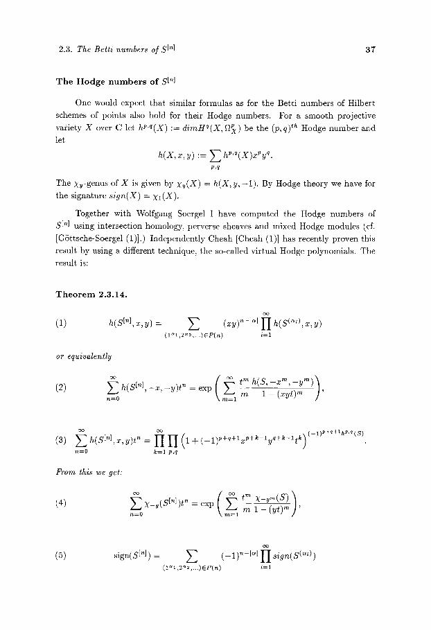
T h e H o d g e n u m b e r s of S [~]
One would expect that similar formulas as for the Betti numbers of Hilbert
schemes of points also hold for their Hodge numbers. For a smooth projective
variety X over C let hP'q(x) := dirnHq(X, ftPx) be the (p,q)th Hodge number and
let
h(x, x, y) := ~ hp,~(X)x%~ P,q
The xy-genus of X is given by xy(X) = h ( X , y , - 1 ) . By Hodge theory we have for the signature ~ig~(X) = ~ ( X ) .
Together with WoKgang Soergel I have computed the Hodge numbers of
S [hI using intersection homology, perverse sheaves and mixed Hodge modules (cf.
[GSttsche-Soergel (1)].) Independently Cheah [Cheah (1)] has recently proven this
result by using a different technique, the so-called virtual Hodge polynomials. The result is:
T h e o r e m 2.3.14.
(1) h(S In], z, y) =
or equivalently
(2)
oo
Z (xy) ~-I~l I I h(s(~'), x, y) ( l ~ l , 2 ~ 2 , . . . ) E p ( n ) i=1
h ( S M , - x , - y ) < = exp -- ~ = ( - ; ~ y ~ , n=0 m = l ~
(3) n~O
oo E h(S[n]'x'y)~n ~ ~Il-I (t -~-(--1)P+q+lxP+k--lyq+k--l~k)(-1)P+q+lhP'q(S)
k = l p,q
From this we get:
(4) x_~(sM)t ~ = exp x-~ (s)
(5) sign(SE~ = F_, (-1)"-I~l [I ~ig~(S("')) (1"1 ,2~ : , . . . ) 6 P ( n ) i=1

38 2. Betti numbers of Hilbert schemes
or equivalently
fI ( 6 ) E sigTt(s[n])tn = ( l -- tkx~ (--1)ksign(S)/2 n=0 k=l \ 1 + t k J (1 -- t2k) - ' ( s ) / : .
(5) and (6) follow from (1) and (3) using sign(S) = XI(~) and e(S) = X- , (S) .
Using these results we can also find formulas for the signatures of Hilbert
schemes in terms of modular forms. Let again v be in the upper half plane and
q = e 2~i~. Let e and 5 be the following functions:
n = l din dd
~=-~-a z q~ n = l d I dd
(cf. [Hirzebruch-Berger-Jung (1)], [Zagier (2) ] . ) , and ~ are modular forms for r0(2) of weights 4 and 2 respectively. Both of them play an important role in the theory
of elliptic genera.
C o r o l l a r y 2 .3 .15.
~-~ sign(S[.])(_q) . = q~(S)/24 ~(w) ~ig"(s) ~=o ~( 2r ) ( ~ig~( s)+~( s) ) /2
= (q)e(S)/24
For a K3 surface we get in particular
oo sign( s N ) ( - q ) . = q A(T)2/3 A(2T)I /3
n=o q z
512e(52 - 6 ) 3 / 2 "
Proof." We set t := - q in 2.3.14(6). Then we get
~ign(st"J)(-q)" = I I \1 + qk ) ( 1 - q~k)-e(s)/~ n = 0 k = l
(1 - - qk)sign(S) = 11 ( 1 - ~ ( ~ S ) ) / 2
k = l
= qe(S)/24 ~/(v) ~ig"(s) 7i( 2~-)( ~ig.( s)+~( s) ) /2

2.3. The Betti numbers of S In] 39
Using the formulas A ( T ) = 4 0 9 6 ~ ( 6 2 - ~)~
~ (~ )16 _ 64(65 _ ' ) ,7(2,-)8
(cf. [I-Iirzebruch-Berger-Jung (1)]) we get
r/(w) "ig'~(s) = (64(62 _ s162 ~( 2T )( , ig.( s)+~( s) ) /~

40
2.4. T h e B e t t i n u m b e r s of h i g h e r o r d e r K u m m e r v a r i e t i e s
D e f i n i t i o n 2.4.1. Let S be a smooth projective variety over an algebraically
closed field. Let as above w,~ : S [~] ----+ S ( ' ) be the Hilbert-Chow morphism. Let
A be the Albanese variety of S and a : S ----* A be the Albanese morphism. Let
aN : S (n) ) A (~) be the morphism induced by a and let gn : A (n) ~ A be the
morphism which maps a zero-cycle ~-][xi] to its sum ~ xl in the group A. We put
/ k ' S n - 1 = a ) n l ( a n l ( g n l ( 0 ) ) ) .
In the following two cases we want to compute the Betti numbers of t h e / x ' S n - l :
(1) S = A is a two-dimensional abelian variety over C; then a = 1A : A - - ~ A, so
we have K A n - 1 = g~l(0). In this case K A n - 1 has been defined in [Beauville
(1),(2),(3)]. There it has also been shown that K A n - 1 is a smooth symplectic
variety, and thus a new family of symplectic varieties was constructed. /x'A1 is
the Kummer surface of A. So we can see the K A n - 1 as higher order Kummer
varieties of A. This is the more impor tant case.
a (2) a : S- - -~A is a geometrically ruled surface over an elliptic curve A.
L e m m a 2.4.2. Let S = A be an abelian surface, or let a : S ----* A be a geometri-
cally ruled surface over an elliptic surface A over C or over 1Fq, where gcd(q, n) = 1.
Then K S n - 1 is smooth.
P r o o f i For an abelian surface this has already been shown in [Beauville (1)]. We
briefly repeat the argument: let (n) : A
have the cartesian diagram
A • K S , - I
l A
This is true because the fibre product is
A be the mult ipl icat ion by n. Then we
, A [n]
[] 1 (n)
~ n .
{(b,Z) e A • A In] I g n ( w , ( Z ) ) = n . b},
and this is isomorphic to A • K S n - 1 via (b, Z) H (b, Z - b). Here Z - b denotes
the image of Z under the isomorphism
- b : A ----* A;
X ~------+ x - b .

2.4. The Betti numbers of higher order Kummer varieties 41
As (n) is @tale, it follows that KAn- I is smooth. The case of a geometrically ruled
surface can be treated by a modification of this argument. Analogously to the above
we have A x K ( A • , ( A x P 1 ) [ ' q
[] l g n ~
(n) A ~ A.
So K(A x P1)n-1 is smooth. Now let S-2-*A be a geometrically ruled suface. Let
(Ui)i be an open cover of A such that a- 1 (Ui) = Ui x P 1 for all i. We can assume that
for every effective zero-cycle ~ of length n there is an i such that supp(~) C Ui x P1.
Let
K ~ - I := { Z E KSn-1 a(supp(Z)) C Ui}.
Then the K i _ l form an open cover of KSn-1 with
.i P1) [~] K(A x Kn_ 1 ~--(Ui x CI P1)~-1. []
We will again use the Weil conjectures to determine the Betti numbers of the
KSn-1. To count the points we will use a result from representation theory, the
Shintani-descent. Our reference for this is [Digne (1)].
De f in i t i on 2.4.3. Let G be a group and {H / a cyclic group of automorphims of
G. Let Gt,<(H I be the semidirect product. Let j be the set-theoretic map
j :G ----* G~<(H);
g ~-~ (g, H).
The H-classes of G are the sets j - l ( c ) , where c runs through the conjugacy classes
of G. (G, H) has the Lang property, if the set of fixed points G g is finite and each
g E G can be written as g = x - i l l ( x ) for an x E G.
Let L be a connected algebraic group over F q , let G = L ( F q ) and F the
Frobenius over Fq . Then (G, F ) has the Lang property by the theorem of Lang.
T h e o r e m 2.4.4. (c]. [Digne (1) Thin 1.4]). Let G be a group and H, H' two commuting automorphism8 of G such that both ( G , H ) and (G,H') have the Lang property. Then
(1) For all y E G we have y - i l l ( y ) e G H.

42 2. The Betti numbers of Hilbert schemes
(2) The map NH/H, : y - i l l ( y ) H yH'(y -1) definies a bijection from the set of
H-classes of G H' to the set of H'-cla~aes of G H.
Def in i t i on 2.4.5. Let S be a smooth projective surface over hTq and
v = ( n l , . . . , n ~ ) = (I~,2~,3~3...)
a parti t ion of n. We write as above Ic~ I := E c~i, and put Iv I := I~1 (obviously
Iv[ = r). As above we denote the set of partitions of n by P(n). We put
and define
by 7~ls[ . l : = 7 . .
i=1
-y. : s [ . ] , s ( " ) ( F q ) ;
((~i),,v), , ~ ] i . ~i i
U s[~] , s(n)(Fq) vEP(n)
By theorem 2.2.4(3) we can assume (maybe after extending F q ) that
IVt(Fq-.)l-- ~ qmr vEP(l)
for all l < n and all m E PC.
L e m m a 2.4.6. For all ~ E S(n)(~'q) we have I ~ 1 ( ~ ) 1 : I~;1(~)1 .
Proof." Let
= ~ ni~i E s(n)(Fq), i=1
where the ~/ are distinct primitive cycles of degree di. Then we have
Iw2~(~)[ = ~ [Vn,(FC, )l i=1
: ~ Z qdi(ni-'#i') i=1 #iEp(ni)
For i = 1 , . . . , r let # i i i
= ( m l , . . . , m l t ~ q )

2.4. The Betti numbers of higher order Kummer varieties 43
be a par t i t ion of hi, and let
V = ( n l , . . . nl~l)
be the union of d /copies of each # / ( i .e . if #~ = (1 ~[ , 2 ~ , . . . ) , then v = (1 ~ , 2 ~ , . . . )
where ~j = }-~i dia}). Let
i--1 {llmi=j}
Let r] be the sequence (rh,rl2,r?3, . . . ) . Then for all w E A ~-I"l the pair (r/,w) is an
element of S[v] and =
In this way we can get all the elements of 7~-1(~). So we have
~ n l ( ~ ) ~"~ E E "'" E q n - ~ d d . ' l plCP(nl) p2EP(n2) p~EP(n~)
= []
For the next four lemmas let q be a pr ime power satisfying gcd(n, q) = 1 and a
let ei ther S = A be an abel ian surface over F q or let S - - ~ A be a geometr ical ly
ruled surface over an elliptic curve A over ~'q. In this case we assume tha t there
exist an open cover (Ui)i of A and isomorphisms a-l(Ui) ~- Ui • P1 over F q . In
both cases we assume that , for all l _< n, all t he / -d iv i s i on points of A are defined
over F q . All these condit ions can be obta ined by extending F q if necessary. Let F
be the geometric Frobenius over F q . We put
try: A(Fq,) ~ A ( F q ) ;
I
x Z F/(x) i = 0
for all l E SV.
L e m m a 2.4.7. trl is onto and II~r/l(x)[ i,~ independent of x E A(Fq) .
P r o o f : We have A(Fq) F = (A(•q)), and A(~q) F' = (A(Fq,)) . Let x E A(Fq,) .
Choose y C A(Fq) satisfying x : F(y) - y (this is possible by the Lang proper ty) .
Then we have NF~ /F : y -- Fl(y)
l--1
= E Fi(y - F(y)) i = 0
= - - t r l ( x ) .

44 2. The Betti numbers of Hilbert schemes
As F t acts a s the identity on A(Fq) , A(~'q) is the same as the set of Ft-classes on
A(~;'q). Thus by theorem 2.2.4 trt is onto. For x E A(aCv~) and y �9 tr[-~(x) the map
z ~ y + z gives a bijection between tr[ -1 (0) and tr~ l(x) []
Let hn = gn(.Fq)oan(.~i~q) : S(n)(.~q) } A(.Fq).
L e m m a 2.4.8. hn is onto and [hn~(X)l is independent of x E A(~'q).
P r o o f i For any part i t ion t, = (n~ , . . . ,n~) = ( 1 ~ , 2 ~ , . . . ) of n let M(v) be the
conjugacy class of the symmetr ic group G(n) whose elements consist of disjoint
cycles of lengths nl . . . . , n~. Then we have
n~ l i a r / ~1
H ic~' c~i! i=1
and ~-~veP(,~) IM(t,)l = n!, as G(n) is the union of the M(v). For a smooth variety
X over F q we put
X(O, v) := h X ( G ~ )' j = l
x(0,n) :: U x(0,~), vEP(n)
X(n) := U X(0, v) x M(v) . vEP(n)
Let (I)x.0 : X(O,n) ----* X( '0 ;
r ni --1 (X I , . . . ,X r ) V-'---+ Z Z Fl(xi )
i=1 /=0
Cx : X (n ) ---* X(");
((z~,..., ~) , m) ~-, r x~)
r A(n) ---* A(Fq) ;
((al,...,a~),m) ~ ~ tr,,(a,). i=l
C l a i m (*) . Ir = n! for all ~ C X(n) (Fq) .

2.4. The Betti numbers of higher order Kummer varieties 45
Proof of (*): Let ~ = ~ i~1 mini E X (n ) (Fq ) , where the {i are distinct primi-
tive zero-cycles of lengths di. The points of ~xl0(~) can be obtained as follows: for
any i let
# i i i i i = ( l l , ' ' ' , / ] . i l ) = ( " l ~ t ' 2 c ~ 2 ' ' ' ' )
be a partit ion of mi, and put # : = ( ~ 1 , . . - , # r ) . Let
/2(~) = ( n l , . , r t l v ( # ) l ) = (1 ~1 , 2~2 , . . . )
be the union of the partitions di �9 #' of dimi (i.e. flj = ~ i a}/d,)" Let
i=1
be a bijection satisfying no(i,u) = dil i and p(i ,u) <_ p(i ,v) for all i <_ r, u <_ v <_ [#i I.
There are
ILgk! i-I,,j"}!
such bijections. For all l E {1 , . . . , ]v(#)]} we choose an xl E X ( F q - , ) satisfying
hi--1 Z rw(x ) : ' lj~i, w~O
where p-l(1) = ( i , j ) . There are di choices for xt. We see that
(~,,..., x,~(,),) e x(o, .(,)),
and we have ( : ~ X , 0 ( X l , . . . , Xlv(#)l ) ~-- ~. All the elements of Oxl0(~), can be obtained
this way, and all the possible choices lead to different elements. Obviously we have
f i r kZ~ = H H (jdi)~'}" k=l i=1 j

46 2. The Betti numbers of Hilbert ~chemes
Thus we get
(lr �9 IM(,- ' ( f f ) ) l ) pEP(ml)x...xP(mr)
c~ k = l ioo----1
#EP(ml)x...xP(rn~) ,~k, k~, I I H oz; , i = l j = l
d ~1
-- n!. ~ ~ 1 .
X i = l j----1 i=1 j = l /
= ,fI 2 ' i---1 ,uiEP(mi) 0~!,]%
j = l
= n ! .
This shows (*).
Let 5 : S(n) , A(n) be defined by being
a(~'q.~ ) : S(Fq.j ) ~ A(Fq-j )
on the factors S(Fq,j ) and the identity on the M(~,). The diagram
s(,~)
A(n)
d~ S , S ( " ) (Fq)
an(Fq)
~A , A(n)(Fq)
A(Fq)
commutes. By lemma 2.4.7. and by our assumptions before lemma 2.4.7 I~- l (x) l
and la-l(~-l(x))l we independent of x E A(Fq). By (*) we have
I h - ' ( ~ ) l = l a - a ( ~ - ' ( x ) ) l / n ! .
Thus the lemma follows. []

2.4. The Betti number8 of higher order Kummer varietie~ 47
For each l �9 zW let A(Fq) t be the image of the multiplication (1) : A ( F q )
A(Fq) .
L e m m a 2.4.9. Let v = ( n l , . . . , n~) be a partition of a number m �9 SV.
a . : A ( F q ) ~ - - * A ( F q ) g c d ( . ) ;
( X l , . - . , X r ) ~ ~-~nixi i=1
i8 onto and I(r~-l(x)l is independent of x �9 A(Fq)gcd(~).
P r o o f i Let x e A(~'q)gcd(,) and y C A(•q) with gcd(v)y = x. Let m ~ , . . . ,m~ �9 2~
satisfying
~-~ mini = gcd(u). i=1
Then we have
and the map
~.((m,~, , m ~ ) ) = x,
f , : ~-1(0) ~ ~- l (x ) ;
( Y l , . . . , Y r ) ~ (Yl -~- mly , . . . , y r -~ - t o r Y )
is a bijection. []
Observe that
bl(S) = 2dim(A) = 4 2 [
in case (1) (S is an abelian surface); in case (2) (A is an elliptic curve).
L e m m a 2 .4 .10.
(1)
[ K S " - I ( F q ) I - IA(Fq) I Z gcd(v)bl(S)qn-]"] IS(~')(Fq)l v----(lal,2a2,...)EP(n) i=l
1 gcd(v)b~(S)z2(,_l,l) (2) -LA(Fq)I
v=(l ~1,2 a2,.. .)EP(n)
\#i =(1B1,2Z2 ,...) e P(cq) 3--1 j~j/~}!

48 2. The Betti numbers of HiIbert schemes
P r o o f i By lemma 2.4.6 we have
IKS~_~(Fq) I = 17~1(h~1(0))1
= ~ I%-l(h~l(0))l �9 vEP(n)
Let ~, = ( n l , . . . ,nl , i ) = ( 1 ~ t , 2 ~ , . . . ) be a part i t ion of n and let
# = ( m l , . . . , m t ) : = ( l a ~ , 2 ~ , . . . )
be defined by ~i = m i n ( 1 , a i ) for all i. Let
f , : S[u] ---* A(Fq) t ;
( (~1 , . . . , ~t), w) ~ (gam~ (aam~ (~1)) , - . . , ga~ t (aa~ t (~t))).
Then the d iagram
r 1~ ~ A(1Fq) t ~" , A ( F q )
commutes. By l emma 2.4.8 and l emma 2.4.9 a~ofu maps S[u] onto A(•q)gcd(v) =
A(Fq)~cd(.), and If;l(~;l(x))l is is independent of x e A(Fq)gcd(,) . As the mul-
tiplication with god(u) is an 6tale morphism of degree (gcd(u)) b~(s) of A to itself, we see
if;-1(~;-1(0))1 _ IsMI IA(Fq)gcd(~)l
(~=~ Is(~,)(F.)I)q,~-I,l(gcd(u ))b,(S)
IA(Fq)I (1) follows by l emma 2.4.6, and (2) follows from this by remark 1.2.4(3) and an
easy calculation.
T h e o r e m 2.4 .11.
(1) Let A be a two dimensional abelian variety over C. Then
p(KA,~-I , z) - - - (1 + z) 4 (gcd(.))4z 2("-I~l) II v(A(~ z)
v=(l"l,2c'2,...)EP(n) i=1
(2) Let S be a geometrically ruled surface over an elliptic curve over C. Then
1 p ( K S , _ I , z) - (1 + z) 2 Z (g~(')) ~z~r l ]v(s (~) , z) -
v=(1 ~1,2 ~2,,..)eP(n) i=1

2.4. The Betti numbers of higher order Kummer varieties 49
(3) In both cases we can also write these formulas as
P ( K S , - a , - z ) = 1
( 1 - z)b,(s) E gcd(u)bl(S)z2(n-I~l) v=(1 c'1,2 '~2 ,...) 6 P (n )
i----1 \ ,u /=(1 ,o [ ,2 i~,...)6p(c~i)j=l
Proof." Let S be either a two dimensional abelian variety or a geometrically ruled
surface over an elliptic curve over C. Let S be a good reduction of S modulo q,
where gcd(q, n) = 1 such that the assumptions of lemma 2.4.7 hold. Then K S n - l i s
a good reduction of KSn-1 modulo q. (3) now follows by lemma 2.4.10 and remark
1.2.2. (1) and (2) follow from this by the formula of Macdonald for p(S (n), z) (see
the proof of theorem 2.3.10). []
In section 2.3 we have obtained power series formulas for the Betti numbers of
the S ['q. We now also want to give power series for the KSn-1. They will however
not be as nice as those for S ['q. We define a new multiplication Q) on the ring of
power series 2g[[z, t, w]] by
zn l tmlw 1. @ zn2tm2w 12 :~_ znx+n=~gmt+m2WgCd(l~, 12)
and extension by distributivity.
Proposition 2.4.12. oo
p(USn-1)e r~=O
- (1 + z)b,(s) w-d-s
1 -'}- w k - -1 -'}- (1 - - z 2 k - 2 t k ) ( 1 - - z 2 k t k ) b = ( S ) ( 1 - - z2~+2tk)]]l k = l w = l
An equivalent formula is o o
T~,=O
_ ( 1 (wA)b' s) (1- z)b,(S) \ dw )
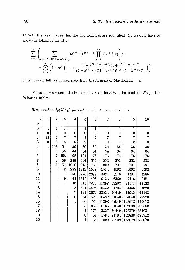
50 2. The Betti numbers of Hilbert schemes
P r o o f i It is easy to see tha t the two formulas are equivalent. So we only have to
show the following identi ty:
n = O v = ( 1 ~1 ,2 ~ , . . . ) E P ( n ) i = 1 , ]
C) ( ( (l + z2k--ltk)bl(S)(1-b z2k+ltk)b3(S) = 1 + w k - 1 + (1 - z 2 k - 2 t k ) ( 1 -- z2k t k )b2 (S ) (1 -- z2k+2t k)
k = l
This however follows immedia te ly from the formula of Macdonald. []
))
We can now compute the Bett i numbers of the KSn-1 for small n. We get the
following tables:
Betti numbers b~(KA~) for
n
v
0 1 2 3 4 5 6 7 8 9 10 11 12 13 14 15 16 17 18 19 20
2 3
1 1 0 0 7 7 8 8
108 51 8 56 7 458 0 56 1 51
8 7 0 1
1
0 7 8
36 64
168 288
1046 288 168
64 36
8 7 0 1
higher order Kummer varieties:
36 64
191 344 915 312 748 312 915 344 191
64 36
7 8
36 64
176 352 786
1528 2879 4496 7870 4496 2879 1528
786 8 352 7 176 0 64 1 36
6 7
1 1 1 0 0 0 7 7 7 8 8 8
36 36 64 64
176 176 352 352 809 794
1584 1592 3327 3278 6136 6360
11298 12202 16432 21704 25524 36440 16432 51640 11298 67049
6136 51640 3327 36440 1584 21704
809 12202
1 0 7 8
36 64
176 352 794
1592 3301 6416
12571 23456 43043 74040
118672 162808 198270 162808 118672
9 10
1 0 7 8
36 64
176 352 794
1592 3286 6424
12522 23680 44142 79920
140073 232368 354034 471712 538070

2.4. The Betti numbers of higher order Kummer varieties 51
Betti numbers bv(KSn) for c u r v e :
6 7 8 9
10 11 12 13 14 15 16 17 18 19 20 21
n 1 I]
0 1 1 0 2 6 3 2 4 6 5 0
1
2 3 4
1 1 1 0 0 0 3 3 3 4 4 4 6 13 10 8 14 16 6 45 4 32 48 3 45 90 0 14 72 1 13 90
4 48 3 30 0 16 1
S a geometrically ruled surface over an elliptic
1 0 3 4
10 16
30 35 54
198 142 247 232 247 142
10 108 4 54 3 35 0 16 1 10
4 3 0
0 3 4
10 16 32 56 97
156 243 348 486 472 486 348 243 156
97 56 32 16
4 10 16 32 56
102 162 278 434 568 892
1206 1232 1206
892 568 434 278 162
1 0 3 4
10 16 32 56 99
164 275 448 711
1C56 1541 2C48 2557 2640 2557 2C48 1541 1C56
1 0 3 4
10 16 32 56 99
164 280 454 738
1146 1763 2590 3643 4704 5737 5984 5737 4704
10
1 0 3 4
10 16 32 56 99
164 277 456 735
1160 1811 2764 4089 5824 7903
10O28 11788 12288
Let al(n) be the sum of the posit ive integers dividing n. For
r E H : = { a + b i E C b > O }
let q := e 2'~i'. Then the eta function and the Eisenstein series E2 are given by
7](7") :---- ql/24 l - I ( 1 _ qn) n~--I
Be(r) := 1 - 24 E (Tl(n)q n. n = l
We put O(r) := q - ' / 2 4 ~ ( r ) .
C o r o l l a r y 2 .4 .13 .
(1) For an abelian surface A over C we have
e ( K A n - l ) ---- n3•l(n).

52 2. The Betti numbers of Hilbert schemes
(2) F o r a geometrically ruled surface over an elliptic curve we have
e (gSn_ 1) = 2ncrl (n).
(3) In both cases this can be expressed in terms of modular forms as
oo Ec(I~-Sn_l )qn 3 - bl(S)/2 ~ q d ~ bl(S)-I d n=i -- 41Ti k dqJ log(iT(T))
= 1 ( 3 - b1(S)/2) \ dq] E2.
P r o o f i As p ( S , - z i) is divisible by (1 - z) b~(s), we see tha t every s u m m a n d
(1 - z)b'(s) i=1 j=l J~ fl}!P( -zJ)~i
in the sum of theorem 2.4.11(3) is divisible by
(1 - z)b'(s)((~,J ~j)-l)
Thus it does not contr ibute to the Euler number , except if u is (n~ ~ ) and #n~ is
(~ - ) for some divisor nl of n. So we get from theorem 2.4.11(3):
nbl(S) nl p(S, - z n/n1) ~(~<s._ , ) : Z - n, ln 1 n (1-z)b~(s) I~=1
(~,,(s) ---- E -bl(S) n l ( 3 - - b l (S) /2) n it 1
nl[n n \ nl /
= (3 -- bl(S)/2)nb~(S)-lcrl(n). []
Table of the Euler numbers (A abel ian surface, S geometr ical ly ruled surface
over an ell iptic curve):
v n 1 2 3 4 5 27,: 7 9 7 4 : 0 10 e(KAn) 24 108 448 750 2592 7680 18000 15972 e(KSn) 12 24 56 60 144 112 240 234 360 264
We can again see easily tha t the Bett i numbers bi(KSn-1) become stable for
i<_n.

2.4. The Betti numbers of higher order Kummer varieties 53
C o r o l l a r y 2 . 4 . 1 4 .
(1 "~- Z 2m'+1 )2bl(S) p(KS._I,z) - ( i -2 ) II f::z-~-z
m=l modulo z n.
Proof:
have For any par t i t ion u of n satisfying [u[ > n/2 we see tha t gcd(u) = 1. So we
p(S [nl, z) p(KSn-1, z) = (1 + z) bds) modulo z ".
Thus we have by corollary 2.3.13
i fi (i + z~m-1)bl(s)(1 + z2m+l) bi(S)
p(KSn-a , z ) - (1 +z) bl(s) ( 1 - - z - - ~ m ~ ( - i - z 2m+2) m~--I
f i (1 + Z2m+l) 2b1(S) = ~=~ (i - ~ w ~ - T~+~)
oo = (I - z ~) I I (I + z~m+') ~b,(s)
m=l (1 -- z2m) b2(s)+2
modulo z n
The result follows. []
In par t icu la r we have ba(KSn-1) = 0 for all n E ZW. In fact the KAn-1 were
proven to be simply connected in [Beauville (1)].

54 2. The Betti numbers of Hilbert schemes
T h e o rb i fo ld E u l e r n u m b e r f o r m u l a
Let G be a finite group acting on a compact differentiable manifold X. Then
there exists the well known formula for the Euler number of the quotient
1 g ~(x/a) = -~, ~ ~(x ),
' ' g E G
where X g denotes the set of fixed points of g E G. If the quotient X/G is viewed as
an orbifold, it still carries information on the action of G. In [Dixon-Harvey-Vafa-
Wit ten (1),(2)] the orbifold Euler number is defined by
1 ~(x, a) = ~ ~ ~(x. n x h) g h = h g
(the sum is over all commuting pairs of elements in G). Now let X be an algebraic
variety. We assume that the canonical divisor Kx/a of X / G exists as a Cartier
divisor. Furthermore we assume that there is a resolution ~G--Z--~X/G satisfying
K ~ * x / a = ~r Kx/c . Then it has been conjectured that
A
e(x,a) = e(x/a).
This formula we will call the orbifold Euler number formula. In the case that the
group G is abelian this conjecture has been proved in [Roan (1)] under certain
additional hypotheses. In [Hirzebruch-Hbfer (1)] some examples of this formula are
studied. First they give a reformulation:
~(x, a) = ~ , e(xg/c(g)). [g]
Here C(g) is the centralizer of g and [g] runs through the conjugacy classes of G.
Hirzebruch and Hbfer consider in particular the action of the symmetric group G(n) on the n th power S n of a smooth projective surface S by permuting the factors.
The quotient is the symmetric power S (~), and w,, : S ['q ~ S ('0 is a canonical
resolution of S ( ' ) . The canonical divisor Ks, is invariant under the G(n) action.
Thus it gives a canionical Cartier divisor Ks(,) on S( ' ) , and it is easy to show that
~ * ( K s ( . ) ) = Kst.~.
So the assumptions of the conjecture are fulfilled, and in fact Hirzebruch and Hbfer
use my formulas (corollary 2.3.11) to prove that
~(s~-]) = e(s -, o(~)) .

2.4. The Betti numbers of higher order K u m m e r varieties 55
Another case in which they check the formula is that of the Kummer surface KA1
of an abelian surface as a resolution of the quotient of A by G(2) = 2g/2 acting by
x ~ - x . We will now generalize this result to the higher order Kummer varieties
K A n - 1 . Let A be an abelian surface. Let
A ' ~ : = { ( X l , . . . , x ~ ) E A n E x i = O } c A ~
with the reduced induced structure. Then A~ is isomorphic to A '~-1. The G(n)
action by permutat ion of the factors of A n maps A~ to itself. So we can restrict
it to A~ and the quotient is A~ n). Let w := COn[Ix'AN_,. Then w : K A n - 1 ~ A~ '0
is a canonical desingularisation of A~ n). The canonical divisor of A~ n) is trivial,
and by [Beauville (1)] KA,~-I is a symplectic variety; in particular we also have
KKA._ , = O. So the conjecture says that e ( K A n - 1 ) = e(A n-a, G(n)) should hold.
For a permutat ion a of {1 , . . . ,n} let
be the parti t ion of n which consists of the lengths of the cycles of a. It determines
the conjugacy class of a. The fixed point set is given by
( A n ) a { ( X l , . ,Xn) �9 d n . } = .. x~,, . . . . xv, for all cycles ( , 1 , . . . , ui) of a
or
= ~ I I A~i (~) i=1
The centralizer C(a) acts by permuting the cycles of a of the same lengths. So we
get
- 1-I i
For
= HA~ ' (~ ) /G(c~ i (a ) ) .
h = (hi , h 2 , . . . ) e 1-[ i
the fixed point set ((An)~') h consists of the ( z l , . . . , xn) �9 A n satisfying zl = x j for
all i , j for which the following holds: either i and j occur in the same cycle of a, or
they occur in two different cycles of the same length l, and these are permuted by
hr. So we get that ((An)~) h = (An) ~ for some 7 �9 G(n) and
((An)~') h = (An) (1 ...... ) --"~ A,
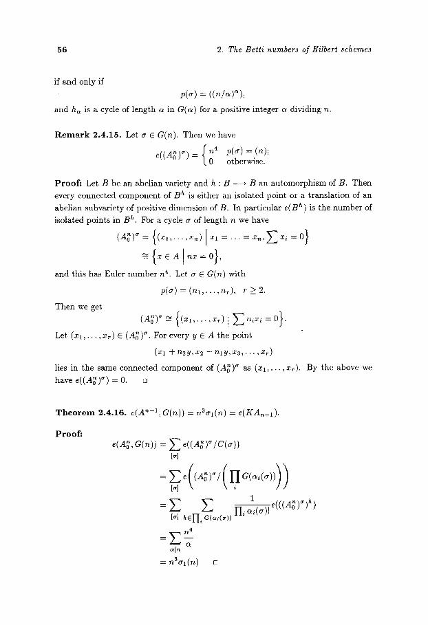
56 2. The Bett i numbers of Hilbert schemes
if and only if p(~) = ((~/~)~),
and ha is a cycle of length a in G(a ) for a posit ive integer a dividing n.
R e m a r k 2 .4 .15 . Let ~r E G(n). Then we have
{n 4 p(~) = (n); e((A~)~) = 0 otherwise.
P r o o f : Let B be an abel ian variety and h : B ~ B an au tomorph i sm of B. Then
every connected component of B h is ei ther an isolated point or a t rans la t ion of an
abel ian subvariety of posit ive dimension of B. In par t icu la r e(B h) is the number of
isolated points in B h. For a cycle a of length n we have
= x E A n x = ,
and this has Euler number n 4. Let a E G(n) with
p(a) = ( n l , . . . , n r ) , r > 2 .
Then we get
(A~)a~ {(Xl,...,Xr) Znix i =0}. Let ( z ~ , . . . ,x~) C (A~) ~. For every y e A the point
(Xl + n2y, x2 - n l y , x 3 , . . . , x r )
lies in the same connected component of (A~) a as ( x a , . . . ,x~). By the above we
have e((A~) ~) = 0. []
T h e o r e m 2.4.16. e(A n-l, C(n)) = n 3 o ' l ( r ~ ) = e(I(An-1).
P r o o f i e(A~, C(n)) = Z e ( ( A ~ ) ~ / C ( a ) )
M
Ili ~(~)! ( ( ( 0 ) ) )
n 4
Mn
= n30" l ( n ) [2]

2.4. The Betti numbers of higher order Kummer varieties 57
Conjectures on the Hodge numbers of the KSn-1
Similar to the results of theorem 2.3.14 we can formulate conjectures on the
Hodge numbers of the KSn-1.
Conjecture 2.4.17.
h ( K S n - l , x , y ) 1
((1 + x)(1 + y))b,(S)/2
�9 1] h(S(~ i
or equivalently
h(KSn-a, - x , - y ) 1
(1 - x)~,(s)/:(1 - u)b,(s)/z
�9 0( , /~' =(I p ,
~_, (gcd(~'))b'(S)(xy) "-H v=(l~t ,2~2 , . . . )EP(n)
g~d(v)~l(s)(x~,) " - H v=(l ' : ' 1,2c'2 ,...)EP(n)
,2~2,...)ep(c~i) J J ~/%. ]
In the case of the KA,_a the conjecture has been verified in [GSttsche-Soergel (1)].
R e m a r k 2.4.18. From the proven part of conjecture 2.4.17 we get for the )/y-genus and the signature:
(1) X - y ( K A , - 1 ) = n E nla(1 + Y"" + yn/nl--1)2yn--n/n,
(2) s i g n ( g A , _ l ) = ( - 1 ) ~ - l n E d3" din , n / d odd
We can again express the signatures of the KAn-1 in terms of modular forms (no-
tations as in 2.3.15).
(3) sign(KAn)(-q) n = ~q. rt~O
Proof." As in 2.4.12 only the terms with u = (n~/n'), #,~In, = (n/nx) give a
contribution to the xu-genus. So we get
x-y(gA._ l ) = ~ ~ ( 1 - x"/"')(1 - ~"/",) ~--1 -,I- (1 - x)(1 y)

58 2. The Betti number~ o] Hilbert scheme~
(1) follows by easy computa t ion and (2) by pu t t ing y = - 1 . (3) is obvious from the
definition of e. []
By applying the same argument to the case of a geometr ical ly ruled surface
over an elliptic curve we get that sign(KSn-1) = O. This was however clear from
the beginning as the dimension of KS~-I is not divisible by 4. It seems remarkable
tha t in all cases the signatures and the Euler numbers can be expressed in terms
of the coefficients of the q-development of modula r forms. For the first few of the
X - y ( K A ~ - I ) we get:
X - y ( K A 1 ) = 2 + 20y + 2y 2,
X-v(KA2) = 3 + 6y + 90y 2 + 6y 3 + 3y 4,
X-y(KA3) = 4 + 8y + 44y 2 + 336y 3 + 44y 4 + 8y ~ + 4y 6,
X-y(KA4) = 5 + 10y + 15y 2 + 20y 3 + 650y 4 + 20y 5 + 15y 6 + 10y 7 + 5y s,
X-y(KA~) = 6 + 12y + 18y 2 + 72y 3 + 288y 4 + 1800y ~ + 288y 6 + 72y 7 + 18y s,
+ 12y 9 + 6y 1~
Let b+ be the number of posit ive eigenvalues of the intersection form on the
middle cohomology and b_ the number of negative ones. Then we get the following
table:
1 2 3 4 5 6 7 8 9 10
b2n(KAn) s ign(KA,)
22 108 458
1046 3748 7870
25524 67O49
198270 538070
-16 84
-256 630
-1320 2408
-4096 6813
-10080 146521
b+(KAn)
3 96
101 838
1214 5139
10714 36931 94095
276361
b-(KAn)
19 12
357 208
2534 2731
14810 30118
104175 251709
We can also determine the Chern numbers of KA2:
C 4 = O, C~C 2 : O, ClC3 : O,
c4 = 108,
c~ = 756,
This is t rue because cl = --KtcA._I = 0 and
sign(KA,_l) = l (7p2(KA2) - p2(KA2)) = 84,

2.4. The Betti numbers of higher order Kummer varieties 59
p~(KA~) = ( ~ - 2~)(IZA~) = - 2 ~ ( K A ~ ) ,

60
2.5. The Bet t i numbers of varieties of tr iangles
Let X be a smooth projective variety of dimension d over a field k. For d _> 3
and n > 4 the Hilbert scheme X['q is singular. However X [3] is smooth for all
d E ~W. In this section we want to compute the Betti numbers of X [3]. X [3] can be
viewed as a variety of unordered triangles on X. We also consider a number of other
varieties of triangles on X, some of which have not yet appeared in the literature.
As far as this is not yet known, we show that all these varieties are smooth. We
study the relations between these varieties and compute their Betti numbers using
the Weil conjectures.
Def in i t ion 2.5.1. [Elencwajg-Le Barz (5)] Let Hil'---b'~(X) C X [~-1] x X In] be the
reduced subvariety defined by
Hil--'bn(X) = { ( Z . _ I , Zn) C X [~-1] • X[~] Zn-1 C Z . }.
~ 3 ~ 3 Here we will be interested in Hilb (X). Let i : Hilb (X) ~ X [2] • X [3] be
the embedding. If one interprets X[ 3] as a variety of unordered triangles on X, then ~ 3 Hilb (X) parametr izes triangles Z3 with a marked side Z2. In the case k = C it was
~ 3 ~ 3 shown in [Elencwajg-Le Barz (5)] that Hilb (X) is smooth. Hilb (X) represents the
contravaria~t functor from the category of Schln k locally noetherian k-schemes to
the category Ens of sets
~ 3 7-lilb (X) : Schln k
T ,
( r ---~ T2) ,
Ens;
, xt l(T) • XE I(T) c
, ( ( z ~ , z ~ ) ~ ( ( i x • r • r
So for a smooth variety X over C and a reduction X0 of X modulo q the variety ~ 3 ~ 3 Hilb (X0) is a reduction of Hilb (X) modulo q. Let
P2 : Hii-b3(X) ----* X [31
be the projection. For any part i t ion • of 3 ( i . e . . = (1, 1, 1), J v = (2, 1), J ~ = (3)
) we put ~ 3 Hilb~(Z) := p~-l(x[~3l).
In [Elencwajg-Le Sarz (5)] a residual point of a pair (Z2, Z3) E ~ b 3 ( X ) is defined.
Def in i t ion 2.5.2. [Elencwajg-Le Barz (5)] Let
(Zn-1, Zn) ~ X [~-1] • X [~].
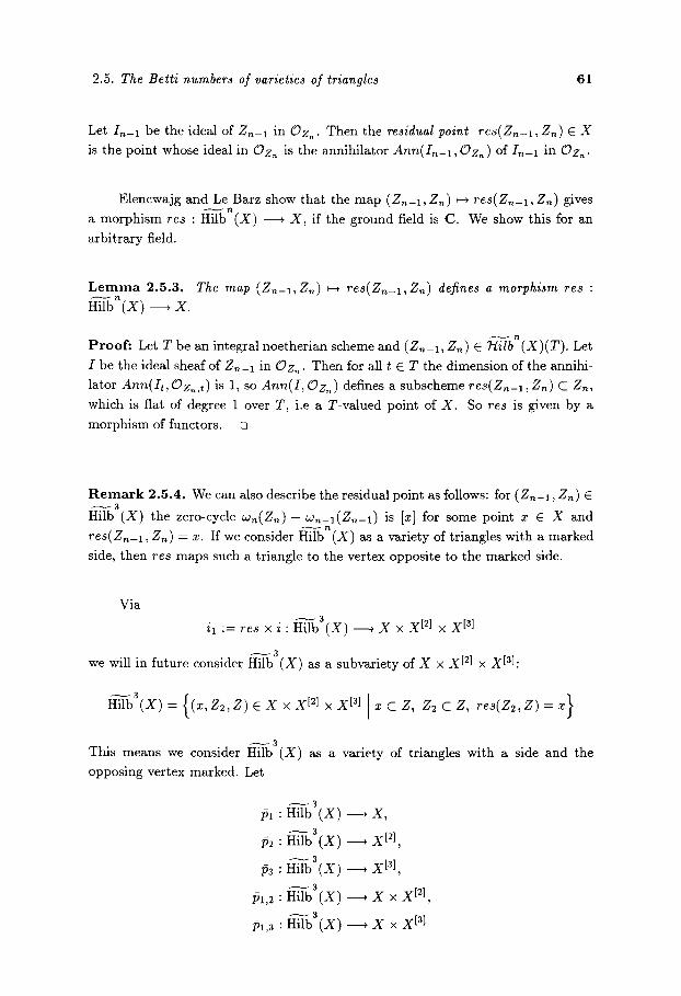
2.5. The Betti numbers of varieties of triangles 61
Let In-1 be the ideal of Zn_ 1 in Oz.. Then the residual point r e s ( Z n - 1 , Zn) E X
is the point whose ideal in Oz. is the annihi la tor Ann(I,,-1, Oz.) of It ,-1 in Oz..
Elencwajg and Le Barz show tha t the map (Zn-a, Zn) ~-* res(Z,_a, Z,) gives ~ n
a morph i sm res : Hilb (X) ~ X, if the ground field is C. We show this for an
a rb i t r a ry field.
L e m m a 2.5 .3 . The map (Z,~-a,Zn) ~ res(Zn-l,Zn) defines a morphism res : ~ n
Hilb (X) ~ X.
~ n P r o o f i Let T be an integral noether ian scheme and (Zn-1, Zn) E 7-filb (X)(T). Let
I be the ideal sheaf of Z,,-1 in Oz.. Then for all t C T the dimension of the annihi-
la tor Ann(It, Oz.,t)is 1, so Ann(I, Ozn) defines a subscheme res( Zn-1, Zn) C Zn, which is flat of degree 1 over T, i.e a T-valued point of X. So res is given by a
morphism of functors.
R e m a r k 2 .5 .4 . We can also describe the residual point as follows: for ( Z n - a , Zn) E ~ 3 Hilb (X) the zero-cycle wn(Zn) - w n - a ( Z , - a ) is Ix] for some point x e Z and
~ n
r e s ( Z , _ l , Zn) = x. If we consider Hilb (X) as a variety of t r iangles with a marked
side, then res maps such a t r iangle to the vertex opposi te to the marked side.
Via ~ 3
i l := res x i : Hilb (X) ~ X x X [2] x X [a]
~ 3 we will in future consider Hilb (X) as a subvariety of X x X [21 x X[3]:
~ 3 This means we consider Hilb (X) as a variety of t r iangles with a side and the
opposing vertex marked. Let
~ 3 t51 : H i l b (X) , X,
~ 3 t52 : H i l b (X) ~ X [21,
~ 3 Pa : Hilb (X) , X [a],
~ 3 Pl,2 : I-Iilb (X) ~ X x X [21,
~ 3 /~1,3 : Hilb (X) ~ X x X [a]
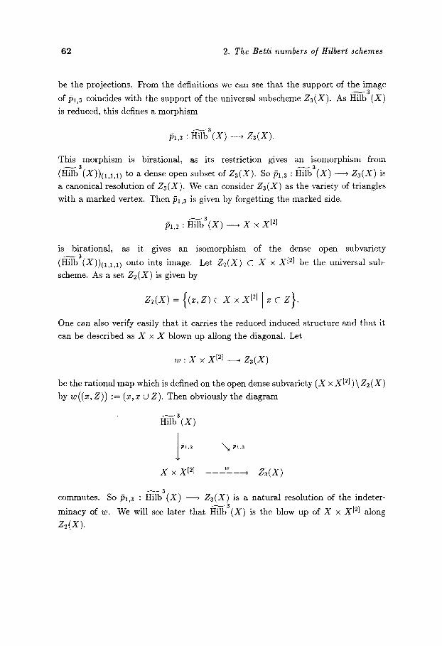
62 2. The Betti number8 of Hilbert schemes
be the projections. From the definitions we can see that the support of the image ~ 3
of/51,3 coincides with the support of the universal subscheme Z3(X). As Hilb (X)
is reduced, this defines a morphism
~ 3
/~1,3 : Hilb (X) , Z3(X).
This morphism is birational, as its restriction gives an isomorphism from ~ 3 ~ 3
(Hilb (X))(1,1,1) to a dense open subset of Z3(X). So/51,3 : ni lb (X) ----* Z3(X) is
a canonical resolution of Z3(X). We can consider Z3(X) as the variety of triangles
with a marked vertex. Then i51,3 is given by forgetting the marked side.
~ 3 P l , 2 : Hilb (X) , X • X [2]
is birational, as it gives an isomorphism of the dense open subvariety ~ 3
(Hilb (X))(1,1,1) onto ints image. Let Z2(X) C X • X [2] be the universal sub-
scheme. As a set Z2(X) is given by
z (x) = x • xc l x c z } .
One can also verify easily that it carries the reduced induced structure and that it
can be described as X x X blown up allong the diagonal. Let
w : X • X [21 ~ Z3(X)
be the rational map which is defined on the open dense subvariety (X • X [2] ) \ Z2 (X)
by w((x, Z)) := (x, x t2 Z). Then obviously the diagram
N 3
Hilb (X)
l lbl ,2
X x X [2] w 4. z (x)
~ 3
commutes. So Pl,3 : Hilb (X) ~ Z3(X) is a natural resolution of the indeter- ~ 3
minacy of w. We will see later that Hilb (X) is the blow up of X • X [2] along

2.5. The Betti numbers of varieties of triangle~ 63
T h e var ie t ies of complete triangles on X.
Semple [Semple (1)] has constructed a variety of complete triangles on P2-
This variety has been studied and its Chow ring was determined in [Roberts (1)],
[Roberts-Speiser (1),(2),(3),(4)], [Collino-Fulton (1)]. (The Chow ring coincides with
the cohomology ring in case k = C). Le Barz has generalized this construction in
[Le Barz (10)] to general projective varieties and shown that the resulting varieties
of complete triangles are smooth. Keel [Keel (1)] also gave a functorial construction
of these varieties. Let X be a smooth projective variety of dimension d over a field k.
We want to define other varieties of complete triangles. Because of this we call the
variety defined by Le Barz the variety of complete ordered triangles on X. We also
want to show that our varieties of complete triangles are smooth by using results fl'om [Le naxz (10)].
Def ini t ion 2.5.5. [Le Barz (10)] Let X be a smooth projective variety over a field
k. The variety H3(X) of complete ordered triangles on X is the closed subvariety of X 3 x (X[2]) 3 • X [3] defined by
(Xl,X2,z3,Z1,Z2,Z3, Z) ~ ( x ) : ~ ( x ~ • (xI~l)~ • xI~l)
Xi,Xj C Zl; Zi C Z; x, : r ~ ( ~ , , Z j ) = r ~ ( Z t , Z )
for all permutations (i ,j , l) of (1, 2, 3)
In [Le Barz (10)] / t3(X) is shown to be smooth for X a smooth variety over
C. H3(X) represents the obvious functor 7~3(X) : Schln k > Ens:
x . xj c z~; z~ c z ; (x1,~2,z3,zl,z2,z3,z) ~t = r ~ ( x , , Z j ) = r ~ ( Z t , Z )
7~3(X)(T) = E (Z 3 x (X[2]) 3 X X[aI)(T) for all permutations (i ,j , l) of (1, 2,3)
(see also [Collino-Fulton (1) rem. (5)]). So if X is a smooth projective variety over
C and X0 is a good reduction of X modulo q, then H3(X0) is a reduction of H3(X)
modulo q. Let j : 9 ~ ( x ) , x ~ • (x~21) ~ • xE31
be the embedding. Let :~1 : ~q3(X) - - ~ X 3,
p~ : 9 ~ ( x ) - - , (x[~]) ~,
b~ : f i - z ( x ) __~ xC~l,
be the projections. From the stratification of X [3] we get one of H3(X). Let u be
a partition of 3. Then we put

64 2. The Betti numbers of Hilbert schemes
We can view the xi as the vertices of the triangle Z and Zi as the side opposite to xi.
Thus s parametr izes the complete ordered triangles on X (i.e. together with
a triangle we are given all its vertices and all its sides together with an ordering).
The projection t51 : H 3 ( X ) -----+ X 3 is birational.
D e f i n i t i o n 2.5.6. [Le Barz (10)] For a pair ( i , j ) satisfying 1 < i < j < 3 let
Z~i, j := {(ZI ,N2,Z3 ) E (X[2]) 3 Zi : Z j} c
be the diagonal between the i th and jth factors. Let
be the small diagonal in X 3, and
~2
the small diagonal in (X[2I) 3. Then we put
E~,j(X) :=/5;~(/x~,~), D~(X) := (/~1 x/52)-1((~1 X (~2).
In [Le Barz (10)] these varieties are shown to be smooth for X a smooth variety
over C. The Ei,j(X) are irreducible divisors in H3(X) . D~(X) is the variety of
second order da ta on X , which we want to s tudy in more detail in chapter 3.
For x 6 X let m x , . be the maximal ideal in the local ring Ox,x and
q. : m x , . ~ mx,~:/m2x,.
'the natura l projection. We can describe the subscheme Z(1,2)(X) C X Is] (cf. section
2.1) as the closed reduced subvariety given by
Z 6 X [3] supp(Z) = x for an x E X, and there is a ]
2-codimensional linear subspace V C rnx,x/m2x,, such that / "
the ideal Iz of Z in Ox, . is of the form Iz = q[ l (V)
Obviously Z(1,2)(X) is isomorphic to the Grassmannian bundle Graas(2, T } ) of two-dimensional quotients of the cotangent bundle of X. We put
E :=/5;~(z(i,2)(x))
[ I supp(Z) -= x; Z1, Z2, Z3 C Z j "

2.5. The Betti numbers of varieties of triangle8 65
Let Z E Z(1,2)(X), x : - supp(Z). Then the ideal Iz of Z in Ox,~ is of the form
Iz = q~-l(V) for a suitable 2-eodimensional linear subspace V of m x , x / m ~ , z. Let
qz : mx,~: ---+ m x , ~ / I z
be the natural projection. The ideals Iz2 of subschemes Z2 of length 2 of Z are given
exactly by the qz I ( W ) for the one-dimensionM linear subspaces W of mx,~ / I z . Let
7r: Z(1,2)(X) = Grass(2, T~) ~ X
be the projection. Then the subschemes Z2 C Z of length 2 are given by the one-
dimensional linear subspaces of the fibre of the tautological subbundle T1 of 7r*(T~)
over the point V. Thus we get
R e m a r k 2.5.7. E ~ P(T1) • . . . . (2,T;r P(T1) XCrass(2,T;r P(T1).
P r o p o s i t i o n 2.5.8. Let X be a smooth projective variety over C. Then
Pl,2 : H~b3(X) ----+ X x Z [2] is the blow up along Z2(X).
Proof : ~ 3
/51,2 : Hilb (X) , X x X[ 2] is an isomorphism over (X x Z [2]) \ Z2(X). Let
F :=/5~,1(Z2(X)). Then F can be described as the set:
: {(X, Z l , g ) E X x X [2] x X [31 x 1 C Z1, Z1 C Z, r e s (Z l ,Z )~ - x 1}. F
Let Pl,4,7 : / ~3 (X) , X x X [21 x X [31
( X l , X 2 , x 3 , Z l , Z 2 , Z 3 , Z ) , "' ( x l , Z l , Z )
~ 3 be the projection. We see immediately that the image of this morphism is Hilb (X)
so we get a morphism
:~,,,~ : ~ ( x ) --~ n~i-b3(X).
Let
(xl, z2, z3, Z1, Z2, Z3, Z) E E1,2(X).
Then we have Z1 = Z2 and thus Xl = x~. So we get Xl C Z1. We see that
P1,4,7(E1,2(X)) C F.
So we get a m o r p h i s m q : E1,2(X) , F. Let ( x l , Z 1 , Z ) 6 F. We put x2 := x~,
x3 := res(xl,Z1). If supp(Z) consists of two points, we see that Xl # x3 and
Z = Z3 tJ x3 for a unique subscheme Z3 of length 2 with support xl. If supp(Z) is a

66 2. The Betti numbers of Hilbert schemes
point but Z does not lie in ZO,2)(X), then Z has a unique subscheme Z3 of length
2. In both cases we get
q--l(xl , Z1, Z) = {(Xl, g2, x3, Zl , Z1, Z3, Z)},
If Z lies in Z(1,2)(X), then it is given by a two-dimensional quotient W of the
cotangent space T~;(xa) of X at xl, and the subschemes Za of Z are given by the
one-dimensional quotients V of W. So we get
q- l (x l ,Z l ,g) = {(.TI,X2,x3,ZI,ZI,Z3,Z ) 23 C Z} "~ P l .
Putt ing things together we see that q is onto and a bijection over the open set
F\paa(Z(1,2)(X)). As Ea,z(X) is an irreducible divisor of s F is an irreducible ~ 3
divisor on Hilb (X). Let
e : X x-'X[~] ---+ X • X [21
be the blow up of X • X [2] along Zz(X). Let Z be the ideal of Z2(X) in X •
--1 OH_~b3(x ) X [2]. From p~(Z2(X) ) = F we get that plaZ. is the invertible sheaf
corresponding to F . By the universal property of the blow up (cf. e.g. [Hartshorne
(2), II. prop.7.14]) there is a morphism
N 3 g : Hilb (X) -----+ X x-X[2]
such that the diagram
~ 3 Hilb (X) ~ , X x'--X [2]
X x X[ z]
commutes, g is a birational mo.. rphism. By [Hartshorne (1) II Thm. 7.17] g is the
blow up of a subscheme of X • X[2]. g is an isomorphism outside F , F is irr__._~educible,
and the image g(F) is the exceptional divisor of the blow up g : X • X[ 2]
X • X [21. Thus g is an isomorphism and the result follows. D
In a joint work with Barbara Fantechi [Fantechi-G6ttsche (1)] we use proposi-
tion 2.5.8 to compute the ring structure cohomology ring H*(X [3], Q) of the Hilbert
scheme of three points on a smooth projective variety X of arbitrary dimension
in terms of the cohomology ring of X. We also compute the cohomology ring of ~ 3 Hilb (X).
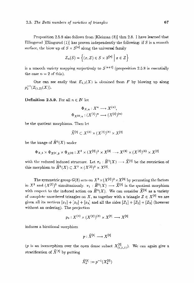
2.5. The Betti numbers of varieties of triangles 67
Proposi t ion 2.5.8 also follows from [Kleiman (3)] t hm 2.8. I have learned that
Ellingsrud [Ellingsrud (1)] has proven independently the following: if S is a smooth
surface, the blow up of S x S In} along the universal family
zo(s) = s • stol x z }
is a smooth variety mapping surjectively to S[ n+l] (proposit ion 2.5.8 is essentially
the case n = 2 of this).
One can see easily that E1,2(X) is obtained from F by blowing up along
p31(zr
D e f i n i t i o n 2.5.9. For all n E zW let
~x,n : X n -----+ X (~),
excel, , : ( X [21)" ---+ (X [21)(")
be the quotient morphisms. Then let
)~[31 C X (3) • (X [2])(3) • X[3]
be the image of H s ( X ) under
~X,3 • ~X[21,3 X ~X[Sl : X 3 • (X[2]) 3 • X [31 ---+ X (3) • (x[2l) (3) • X [3]
with the reduced induced structure. Let ZCl : H 3 ( X ) ~ .~[3] be the restriction of this morphism t o / I 3 ( X ) C X s x (X[2]) 3 x X [3].
The symmetr ic group G(3) acts on X 3 • (X [2])3 • x[3l by permut ing the factors
in X 3 and (X[2]) 3 simultaniously. 7rl : H3(X) ~ 2 [3] is the quotient morph ism
with respect to the induced action on ~r3(X). We can consider )~[3] as a variety
of complete unordered triangles on X, as together with a triangle Z E X [3] we axe
given all its vertices [xl] + Ix2] + [x3] and all the sides [Z1] + [Z2] + [Z3] (however without an ordering). The projection
P3 : X (3) • ( X ( 2 ) ) (3) x X [3] ~ X [31
induces a birational morphism
p : )~[31 ~ X[3]
(p is an isomorphism over the open dense subset Y [3] ) We can again give a ( 1 , 1 , 1 ) �9
stratification of )~[3] by put t ing
L31 := p-l(x 31)

68 2. The Betti numbers of Hilbert schemes
for all partitions v of 3. We put
F_~ :~. p-l(z(1,2)(X))
f ( a [ 4 , [ z , ] + [ z , ] + [ z ~ l , z ) x ~ x ; ZI,Z2,Z3 ~ X[2]; a E Z<l,2)(X); / / supp(Z) = x; Z1, Z2, Z3 C Z ~
Then we have /) = rq(E). The action of G(3) on -~3(X) maps E to itself. The
induced operation of G(3) on E is by permuting Z1, Z2, Za a n d / ) is the quotient .
So we get from remark 2.5.7:
R e m a r k 2.5.10.
---- (P(T~) • P(T,) • P(T1))/G(3)
= P(Syma(T1)).
P r o p o s i t i o n 2.5.11. Let X be a smooth projective variety over C. Then
(1) 2{ai is smooth.
(2) p : 213J ~ x{31 i~ the bto~ up aZong Z(~,2)(X).
Proof i It is clear that p is an isomorphism over the open dense subset (X[a])(x,xj). g[3] i.e. Let Z = (Z2 U x) E "'(2,1),
r[21 Z2 E "'(2),
Then we have
Now let
x E X, y := supp(Z2) 5~ x.
p-'tz)= {(2[yl+[4,2t(xuyll+[zcz)}.
( .g[a} \ Z ~ \==(3) ~-Z(1,2)(x)) = Z(1,1,1)(X)
and x := supp(Z). Then the ideal of Z in Ox, , is given by
I z = ( * ~ , x 2 , . . . , x d )
for suitable local parameters Xl, x2 , . . . , xa. The subscheme Z2 given by
is the only subscheme of length 2 in Z, and we have
p-l(z = {(3L 1,3Ez21, z)}.
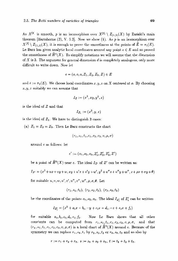
2.5. The Betti numbers of varieties of triangles 69
As X [3] is smooth, p is an i semorphism over X [31 \ ZO,2)(X ) by Zariski 's main
theorem [Hartshorne (2), V. 5.2]. Now we show (1). As p is an i somorphism over
X [3] \ Z(1,2)(X), it is enough to prove the smoothness at the points o f /~ = r l ( E ) .
Le Barz has given analyt ic local coordinates a round any point e E E and so proved
the smoothness of J~a(X). To simplify nota t ions we will assume tha t the dimension
of X is 3. The argument for general dimension d is completely analogous, only more
difficult to wri te down. Now let
E = ( o , o , o , Z l , Z 2 , Z 3 , Z ) c: E
and g := 7r 1 (E). We choose local coordinates x, y, z on X centered at o. By choosing
x, y, z sui tably we can assume tha t
is the ideal of Z and tha t
Iz := (x 2, xy, y~, z)
Iz, := (z ~, y, z)
is the ideal of Z1. W'e have to dis t inguish 3 cases:
(a) Z1 = Z2 = Z3. Then Le Barz constructs the chart
( r l , 81, t l , (31, C2, C3, V, p, IT)
around e as follows: let
r := (ol, o~, o3, Zl, Z~', Z;, Z')
be a point of .~3(X) near e. The ideal Iz, of Z ' can be wri t ten as:
Iz, = (x~ + u x + v y + w , x y + u ~ x + v t y § + u " x + v ' y W w " , z + p x + a y + O )
for sui table u, v, w, u ~, v ~, u", v", w", p, a, O. Let
(r l ,81 , t l ) , (r2,8~,t~), (r3,83,t3)
be the coordinates of the points Ol, o2, o3. The ideal Iz~ of Z~ can be wri t ten
Iz~ = (x 2 + aix + b i , - y + cix + di, - z + eix -I- f i )
for sui table ai, bi,ci,di, ei , f i . Now Le Barz shows tha t all other
constants can be computed from r l , s ~ , t l , c l , c 2 , c a , v , p , a , and tha t
( r l , Sl, t l , e l , c2, c3, v, p, (7) is a local chart of H 3 ( X ) a round e. Because of the
symmet ry we can replace r l , s l , t l by r2 ,s2 , t2 or r3,s3,t3 and so also by
r : = r l -l-r2 + r 3 , 8 := 81 -I-82-t-83, t : = t l - t - t2- l- t3.

70 2. The Betti numbers of Hilbert schemes
(b)
(c) The Zi are pairwise distict.
are of the form
So we get the local chart (r , s , t , c l , c2 , c3 ,v ,p ,a ) around e. With respect to
this chart the action of 7" C G(3) on ~r3(Z) is given by
~( r ) = r, ~(~) = 8, ~( t ) = t,
r(ci) = c~(i),
T ( v ) = ~, ~ ( p ) = p, ~ ( o ) = ~ .
So we see that (r ,s , t , cl + c2 + c3,clc2 + cac3 + c2c3,cac2c3,v,p,a) are local
coordinates of )~[3] around ~.
Za = Z2 # Z3. In this case we can choose the local coordinates x, y, z in such
a way that the ideal Iz3 of Z3 is given by
I z , = (x 2, y - x, z).
So the ideal Iz~ of Z~ is of the form
Iz, s = ( x 2 + a x + b , - y + ( 7 + l ) x + d , - z + e x + f ) .
By [Le Barz 10] (r, s, t, Cl, c2,7, v, p, a) are local coordinates around e. The
stabilizer of the operation around e is G(3)e --= {1, (1,2)}. We can choose the
coordinate neighbourhood so small that we have
~(Y) n U # 0 *=* ~ G ( 3 ) e .
r, s, t, 7, v, p, a are fixed by the action of G(3)r and we have
( 1 , 2 ) ( C 1 ) = C2, (1 , 2 ) (C2) = C 1,
So (r, 8, t , cl + C2,ClC2,7, v,p,o') form a local chart of )~[3] at ~.
We can assume that the ideals Iz2, Iz~ of Z2, Z3
Iz2 = (z 2, - y + x, z),
Iz~ = (x2 ,z + y,z).
Then the ideals Iz~, Iz, 3 of Z~, Z~ can be written in the form
Iz~ = (z 2 + a2x + b 2 , - y + (7 + 1)x + d 2 , - z + e2x + f2),
Iz, a = (x 2 + a3x + b 3 , - y + (7' - 1)x + d 3 , - z + e3x + f3)-
Le Barz shows that (r, 8, t, cl, 7, 7 ' , v, p, a) form a local chart of H3(X) around
e. The stabilizer of the action of G(3) at e is G(3), = {1}. Again we can
choose the coordinate neighbourhood around e to be so small that we have
r(U) n V #O r r = l .

2.5. The Betti numbers of varieties of triangles 71
Then (r,s,t, cl ,7,7' ,v,p,a) is also a local chart of )~[31 at ~. Put t ing things
together we have proved (1).
We already know from remark 2.5.10 that /) := p-I(Z(~,2)(X)) is a locally
trivial Pa-bundle over Z(~,2)(X) = Grass(2, T}). In pa r t i cu la r / ) is an irreducible
divisor on )~[3]. So we can complete the proof of (2) in the same way as that of
proposition 2.5.8. []
Keel [Keel (1)] has proved by a different method that the symmetric group
G(3) acts on Ha(X) and that the quotient is the blowup of X [a] along Z(1,2)(X).
Let ~ 3 Hilb (X) C X x X (2) x X [21 x (X[2]) (2) x X [a]
be the scheme-theoretic image of .~a(X) under 1x x ~I'x,2 x lxE~l x ~xE2~,2 x 1xE~I and let
:r2: H3(X) , Hil"'b3(X)
be the restriction of this morphism. 2g/22g acts on X a x (X [21 )a .x X [a] by permuting
the last two factors in X a and (X [~] )a simultaniously. This action restricts to an
action on Ha(.X). Let 7r2 : Ha (X) , Hil""ba(X) be the quotient morphism. ~rl
factorizes into ~ 3 ( x ) ~1 , ~E31
~ 3 Hilb (X).
~ 3 We can view Hilb (X) as the variety of complete triangles on X with a marked
vertex (or equivalently with a marked side). The projection
Pl,3,5 : X x X (2) x X [21 x (X [2])(2) x X [31 ~ X x X [2] x X [3]
restricts to a birational morphism
~ 3 ~ 3 ~1,3,~: Hilb (X) , Hilb (X).
~ 3 Let 10a : Hilb (X) , X [31 be the projection. We put:
~ 3 B(X) := ~;1(Z(I,2)(X)) C Hilb (X)
with the reduced induced structure. B(X) is a P l -bundle over Z(1,2)(X) ----
Grass(2, T~c). In fact we can see in the same way as above that B(X) = P(T1)
holds, where T1 is the tautological bundle on Grass(2, T} ). We put
/~ := !~I,~(B(X))
f(x,2[x],Zl,[Z2] t-[Z3],Z) x ~ X; Zi,Z2,Z 3 ~ 2[2]; Z ~ / ( 1 2 ) (2 ) ; "~ / s u p p ( Z ) = x; Z1, Z2, Z3 C Z' f

72 2. The Betti numbers of Hilbert schemes
Then we have / ) = ~r2(E). The action of 2g'/2Zf on hr3(X) restricts to an action on
E by permuting Z2, Z3, and the quotient i s / ) . So we get from remark 2.5.7:
R e m a r k 2 .5 .12 .
/) ~ (P(T1) x c . . . . (2,T7r P(T1) • . . . . (2,T~r P ( T 1 ) ) / ( 2 Z / 2 , ~ )
= P(T1) x c . . . . ( 2 , T } ) P(Sym2(T1)),
and the restriction 151,a,s : / ) ~ B ( X ) is the projection onto the first factor.
P r o p o s i t i o n 2.5.13. Let X be a smooth projective variety over C. Then
~ 3 (1) Hilb (Z) is smooth.
~ 3 ~ 3 (2) Pl,a,s : Hilb (X) - -~ Hilb ( X ) is the blow up along B ( X ) .
~ 3 Proof : /51,3,5 is obviously an isomorphism over Hilb (X) (1 j j ) . Let (x, Z2 ,Z) E ~ 3 Hilb (X)(2,1). Then there are two cases:
(c 0 Z2 = x U y for a point y :fix and Z = 1472 U y for a subscheme W2 of length 2
with supp(W2) = x. Then we have
Pl,3,5((z, Z 2 , Z ) ) = x , [ x ] 4 - [ y ] , x U y , [ x U y ] 4 - [ W 2 ] , W 2 U y �9
(fl) supp(Z2) : y # x. Then we have
Z ,Zl) = { z ,2[x u u } Now let
~ 3 (x, Z2, Z) C Hilb (X)(3) \ B ( X ) .
Then Z2 is the only subscheme of length 2 contained in Z. So we have
~--1 {( } Pl,a,5((x, Z 2 , Z ) ) .= x ,2[x] ,Z2 ,2[Z2] ,Z) .
~ 3 ~ 3 As Hilb (X) is smooth, this shows that/51,a,s is an isomorphism over Hilb ( X ) \
B ( X ) . We now show (1). As above we only have to show the smoothness of ~ 3 Hilb (X) in points of/~. We again use the local charts of Le Barz around a point
e = (o, o, o, Z1, Z2, Z3, Z) C E. Let g := 7r2(e). We use the same notations as in proposition 2.5.11. There are four cases:
(a) Z1 = Z2 = Z3. We see anologously to the proof of proposition 2.5.11 that ~ 3
(r, s, t, cl , c2 + c3, c2c3, v, p, a) form a local chart of Hilb (X) around ~.

2.5. The Betti numbers of varieties of triangle~ 73
(b) Z1 # Z2 = Z3. We switch the role of Z1 and Z3 in the case (b) in the proof of
proposi t ion 2.5.11. So we see immedia te ly that (r, s, t, ^{, c2 + c3, c2c3, v, p, a)
form a local chart a round ~.
(c) Z1 = Z2 ~ Z3. We switch the role of Z1 and Z2 in (b) in 2.5.11. This way we
see that (r,s,t , cl ,7, c3,v,p,a) form a local chart at ~.
(d) Z1, Z2, Za are pairwise dist inct . Then (r, s, t, c l , 7, 7 ' , v, p, a ) form a local chart
near ~.
We have proved (1). By remark 2.5.12 E - - ~ B(X) is a locally tr ivial P2- ~ 3
bundle. In p a r t i c u l a r / ~ is an irreducible divisor on Hilb (X) . Now (2) follows in
the same way as in the proof of 2.5.8 and 2.5.11(2). []
If we put our results together, we get the following d iagram for the tr iangle
varieties of a smooth project ive variety X.
x a , P~ ~ ( x )
X x X (2) , Z3(X) , p~,~ ~ 3 p ..... ~ 3 Hilb (X) , Hilb ( Z )
l l TM
X (a) ~ ~, X[3] ~ P ~[a]
Here the horizontal arrows are b i ra t ional morphisms.

74 2. The Betti numbers of HiIbert schemes
C o m p u t a t i o n o f t h e B e t t i n u m b e r s o f s o m e o f t h e s e v a r i e t i e s
To compute the Betti numbers of some of these varieties we will again use the
Weil conjectures. So we have to count their points over finite fields. F i rs t we look
at the local s i tuat ion. Let k be a field and R = k[[xl,..., Xd]]. As above Hi lb"(R)
parametr izes the ideals of colength n in R.
D e f i n i t i o n 2 .5 .14 . For all l E zW let W~ C (Hilb2(R)) z x Hilba(R) be the reduced
closed subscheme defined by
= ~(Ii , . , . , I t , .])E(HilbZ(R)) ' x H i l b a ( R ) I , , . . . , I t D J / . w; ( )
Now let k be a finite field F o.
L e m m a 2 .5 .15 . There is a finite field extension FQ of ~'O such that for all finite extensions ~'q of ~'Q:
( 1 - q d - 1 ) ( 1 - qd) (1 qd-1 1 -- qd Iw~(F~)I= il--q--~-q~ "-+q)'+ 1-q ( 1 )
In particular
(2) i w O ( F q ) l = (1 - q d ) ( 1 - qd+l) iT- l '
I w ~ ( F q ) l - (1 - qd)2
5 - ? V ' I w ~ ( z % ) l = (1 - ( ) ( 1 + 2q + q2 _ 3 ( - ( + 1 )
( 1 - q )2
P r o o f i We have the s trat i f icat ion
Hilba(R) = Z(1 ,1 ,1 ) [-J Z ( 1 , 2 ) .
Over the algebraic closure F q , the s t r a t u m Z(1 ,1 ,1 ) is a fibre bundle over Pd-1
with fibre A d-1. We choose the extension ~b-'Q in such a way tha t the fibre bundle
s t ructure and a tr ivializing open cover are a l ready defined over F Q . Now let ~'q be
a finite extension o f /FQ. Let m = ( z l , . . . , Zd) be the maximal ideal in R. An ideal d I E Z(1,2)(~Tq) corresponds to a 2-codimensional l inear subspace of ( m / m 2) = Lb~q.
So we have
Z(1,2)(Fq) ~ Grass(2, F~).
An ideal I E Z(1,1,1)(Fq) is contained in a unique ideal I ~ = I + m 2 of colength 2 in
R. Let I E Z(1,2)(Fq). Let f : m ~ m / I be the canonical project ion. Then the

2.5. The Betti numbers of varieties of triangles 75
ideals of colength 2 in R containing I are those of the form f - 1 (V) for V e P ( m / I ) . So we get
iWg(Fq) I = [Z(1,2)(X)(Fq)I( 1 4- q)t 4- [Z(1,1,1)(X)(Fq)[.
(1) follows. (2) follows from (1) by an easy computat ion. G
From now on let /F'Q be as in 2.5.15 and let .~itPq be a finite extension of F Q .
Let X be a smooth projective variety over F q .
D e f i n i t i o n 2.5.16. We write V~ instead of Hi lbn(R) (Fq) and put
T 1 l= X ( F q ) ,
T2 := {M c X(IFq) [MI = 2} U P2(X, Fq) U (X(Fq) x V2),
Ta := { M C X ( F q ) IMI = 3} u (X(Fq) x P2(X,~'q)) u Pa(X, F q )
[--J { { X l , ( x 2 , b ) } Xl r x2 ~ X ( ~ q ) , b ~ g2 } [.J (X(~i 'q) x g3) �9
Recall the notations from 2.3.6. We identify a map f : P(X, Fq) ----+ V(.~gq) with
the set
{(~,/') E P ( X , ~ q ) X ( V ( F q ) \ Vo (Fq) ) f (~ ) = I }
and the set M x VI(Fq) with M. In this way T2 is identified with T2(X,_Fq) and
T3 with T3(X, Fq) (see definition 2.3.6). Via these identifications the relation C
carries over to T1, T2, T3. So by 2.3.7 there are bijections
r = 1x(Fq) : X ( F r ' T1,
r : x I 2 l ( F q ) ~ T2,
r : X[3I (Fq) ----* T3,
respecting C.
L e m m a 2 . 5 . 1 7 .
d-1 (1) Ixt3](G)l = Ix(3)(Fq) I + q k ~ l X ( F q ) l 2
- q
4- q2 (1 -- qd-1)(1 -- qd) Y( ~ ,, ( ~ _~ q--~ -- q q , . t, .l~ q ) [ ,
~ 3 _ d-1 (2) IHilb (X)(Fe)I = I(X x X(2))(Fq)I 4- 2qllq~qlX(Fq)[ 2

76 2. The Betti numbers of Hilbert schemes
(3)
q_ q2 (1 -- qd-1)2
t~ r3(x ) (Eq) l = l X 3 ( F q ) l + 3 q = l ~ q IX(Eq)l u
( 1 - qd-J)(1 + 3q _ 3qd _ qd+l + q ) [x (zv~) l .
( 1 - q)2
Proof : Immediately from the definitions we get
~ 3 (~2 • e3)(Hilb (X)(1Fq))=
{x],x2}, {Xl,X2,Xa}) pairwise distinct
v ( z ( ~ q ) • P ~ ( X , ~ ) )
U{({ZI,Z2},{(xl,b),x2}) X, # X2 e X(.~q) be V2}
and
((1X(E,)) 3 x Cz a • r =
{ Xl 'X2'xaeX(~q)} (Xl,X2,x3, {x],x2}, {x2,xa}, {xa,x,}, {Xl,X2,X3}) pairwise distinct
U { ( x l ,Xl,X2,{Xl,X2},{Xl,X2},(Xl,b),{(xl,b),x2}) t xl ~ x2b e V2 e X(Fq) , }
I
U{(x 2 , Xl , Xl,(Xl.,b),{Xl,X2},{xl , x2},{(Xl,b),x2}) x I ~X2ebe w2X(.~q),}
o ( . , x , x , ( x , ~ ) , ( . , < ) , ( x , ~ ) , ( x , c ) ) b~ >~, ~ >c, < >e "
~ 3 We sum the numbers of elements of Ta, (r • e3)(Hilb (X) (~q) and (13(Eq) x r x
ea)(/ta(X)(/Fq)) respectively. Then we use remark 1.2.4 and lemma 2.5.15 to get
IX[3](~q)[ = ( ] X ( f q)l) -~-IP2(X, ff2q)l[X(.~q) I -}-[P3(X,-~q)[
1 - qd + ~ _ q X(Eq)I(IX(~'q) I - 1)
( 1 - q~)(1 - q~+~) ix (E~) l , + (1 - q)(1 - q~)

2.5. The Betti numbers of varietiea of triangles 77
~ 3 ( I X ( f q ) l ) IHilb ( X ) ( . ~ ? q ) l = 3 ~- I P 2 ( X , JFq)IIXOFq) I
1 a - d ( 1 - q d ) 2 + 2-;~:IX(.Fq)I(IX(JFa) I 1 _ ( / - I) + ~ 7 ~ I X ( ~ ) l ,
I~r~(x)(F~)l 1-- d
= 6 ( I X ( f q ) l ) + 3 ~ q q l X ( F q ) ] ( l x ( . ~ ' q ) l - 1) (1 - qa)(1 + 2q + q2 _ 3qd _ qd+l) + IX(Fq)l .
( 1 - q ) 2
By remark 1.2.4 we have
I X ( 2 ) ( F q ) l =
So we get
+ IP~(X, Fq)IIX(F~)I + IPz(x, Fa)l ,
+ IP~(X~)l.
1 - qd IX[3](Fq) I _- IX(~)(Fq) I + k -~ _-q
+ ( ( i - qd)(1 - qd+l) ~- _- q--~-i ~- q~-
- - - 1) Ix (F~) I z
1-r l - - q / l x (F~ ) l ,
- - 3 ( 2 1 - q d ) IHilb ( X ) ( F q ) I = IX(2)(Fq)IIX(Fq)I + k 1 ~ q 2 [X(Fq)I 2
( ( 1 : q d ) 2 21--qd~ + \ (1 - q)2 + 1 - 1 - q / IX(Eq)l ,
( 31 _ qd _ 3 ) IX(Fq)l 2 1Lr3(X)(Fq)l -- lx(l~q){3 '~ ~ 1 - q
+ ( ( 1 - qd)(1 + 2q + q2 _ 3qd _ qd+l)
( 1 - q)2
and the result follows by an easy calculation. []
31 - qd~ + 2 - 1_-77 / [x(F~)I,
T h e o r e m 2.5 .18. Let X be a smooth projective variety over C. Then we have:
(1) p(X [a] , z) = p (X (3), z) + z 21 - z 2d-2 1 - z 2 p(X,z) 2
__ z 2 d - 2 ~ l ~ __ 2d + )p(X,z), - ) ( - )
1 X 1 a p(X E~1, - z ) = ~ p ( X , - z ) ~ + ~p( , - z2 )p(X ,z ) + ~ p ( X , - z )

78 2. The Be t t i numbers of Hilbert schemes
1 - z 2d-2 + z 2 - - p ( X , - z ) 2
1 - z 2
(1 - z Z d - 2 ) ( 1 - z 2~) + z 4 p ( X , - z ) ,
(2) p ( Z [31 , z) = p ( X (3), z) + z 2 1 - z 2d-2 1 - z 2 p ( X , z ) 2
+ z2 (1 - Y - 2 ) ( 1 + z 2 - z 2~ - z 2 d + 2 ) p ( X ' z ) ,
(1 - z 2 ) 2
p ( )~ [a ] ,_z ) = 1 1 X l p ( x , - z a ) - ~ p ( X , - z ) 3 + ~p( , - z 2 ) p ( X , z) +
1 - - Z 2 d - 2 + z 2 - - p ( X , - z) 2
1 - z 2
+ z2 (1 - z ~ d - 2 ) ( 1 + z 2 - z 2d - z 2d+2) ( 1 - z 2 ) ~ p(X,-z),
3 Z 2 d - 2
(3) p (Hi lb ( X ) , z) = p ( X , z) • p ( X (2), z) + 2z 21 - 1 - z 2 p ( X , z ) 2
(1 - z 2 d - ~ ) 2
p(Hi lb ( X ) , - z ) = ~ ( p ( X , - z ) 3 + p ( X , - z 2 ) p ( X , - z ) )
+ 2z 2 1 - z 2d-2 (1 - z2d-2) 2 1 - z2 P(X,z) + z 4 . p ( X , - z ) ,
3 z 2 d - 2
(4) p (Hi lb ( Z ) , z) = p ( X , z) x p ( X (2), z) + 2z 2 1 - 1 - z 2 p ( X , z ) 2
+ z2 (1 - z2d-2)(1 + 2z z -- 2z 2d -- z2d+2)p(X ' z) , ( 1 - z2) 2
p (Hi lb ( X ) , - z ) = p ( X , - z ) 3 + p ( X , - z 2 ) p ( X , - z ) )
+ 2z 2 1 -- z 2d-2 1 - z 2 p ( X , - z ) 2
+ z2 (1 - z2d-2)(1 + 2z 2 -- 2z 2d ~2d+2~ - ~ J p ( X , - z ) ,
(1 - z 2 ) 2
(5) p ( H 3 ( X ) , z ) = p ( X , z) 3 + 322 1 - z 2d-2 1 - z 2 p ( X , z ) 2
+ z2 (1 - z2d-2)(1 + 322 - 3z 2d - z2d+2)p(X ' z) .
(I - z ~ ) 2
P r o o f i X is def ined over a f in i te ly g e n e r a t e d r ing ex tens ion T of 2~, i.e. t he re
is an X T over spec (T ) sa t i s fy ing Z T X T C =- X . Let Y = X T X T ( T / m ) be a ~ 3 ~ 3
good r educ t i on of X m o d u l o q. T h e n y[3], Hi lb (Y) and / ~ 3 ( y ) X[3], Hi lb ( Z )
and H 3 ( X ) are also r educ t ions m o d u l o q, and we can choose the m a x i m a l ideal
m E spec (T ) in such a way t h a t t hey are all good r educ t ions (see the r e m a r k s

2.5. The Betti numbers of varieties of triangles 79
before theorem 1.2.1). Choose m in such a way that fur thermore l emma 2.~15
holds. Then (1), (3) and (5) follow immediately from lemma 2.5.17, remark 1.2.2
and Macdonald 's formula. Z(~,2)(X) is a Grass(2, d)-bundle over X. So we have
(1~1 z2d-2)( 1 _ z 2d) p(z(1,~)(x)) = - -~)-5-z~ p ( X , z )
By proposit ion 2.5.11 w e get
(1 -- z2d-2) (1 -- z2d)l 2 Z4 z6)p(X,z) . p(2t31z)=p(xE~Jz)+ ( ~ : ~ - ~ / : z ~ ~ + +
So (2) follows from (1) by an easy computat ion. B ( X ) is a P l - b u n d l e over Z(1,2)(X). So we have by proposit ion 2.5.13
A ~ ~ : z~ -~ ) ( l_ -_z~ )~z~ z4 )p (X , z ) p(Hilb ( X ) , z ) = p(Hilb ( X ) , z ) + ( I + z2)(1(1 _ z2)( 1 _ z4 ) , +
(4) follows again by an easy computat ion. []
For a smooth projective surface S over C these formulas can be wri t ten as
follows:
p ( S [3] , Z) : p ( S (3), Z) -Jr- z2p(S, Z) 2 -4- z4p(S, Z) ~ 3
p(Hilb (S) = p(S • S (2), z) + 2z2p(S, z) 2 + z4p(S, z)
p(~[31, z) = p(S (~), z) + z~p(S, z) ~ + (z ~ + 2z 4 + z~)p(S, ~) ~ 3
p(Hilb (S), z) = p(S x S (2), z) + 2z2p(S, z) 2 + (z 2 + 3z 4 -{- z6)p(S, z)
p(.f f~(s), ~) = p(S, ~)~ + 3z~p(S, z) ~ + (z ~ + 4z ~ + z~)p(S, z)
Now we consider the case of projective space Pd. The Chow groups Ai (P [3])
and Ai (H3(pd) ) have already been determined in [Rossell6-Xambo (2)].
Propos i t i on 2.5.19. p[3], ~[3], - - 3 d d Hilb (Pal), H~b3(pd) and _~3(pd) all have a cell
decomposition. In particular for Y one of these varieties H2i+I(Y, 2Z) = O; the groups Ai (Y) = H2i(Y, 2~) are free, and their ranks can be computed by theorem 2.5.18.
Proof." Let To,.. . ,Td be homogeneous coordinates on Pd . For i = 0 , . . . n let Pi be the point for whichTi = l a n d T j = O f o r i # j . Let r C S l ( d + l , C ) be the
maximal torus of diagonal matrices and let A0, . . . , Ad be the linearly independent
characters o f t for which any g E I" is of the form g = diag(Ao(g),. . . , Ad(g)). Then F
acts on Pd by g. Ti := Ai(g)Ti. The fixed points are p0 , . - - ,Pd . We have an induced

80 2. The Betti numbers of HiIbert scheme~
action of P on p~n] for all n, as F acts on the homogeneous ideals in To,... ,Td. A subscheme Z E p~n] is a fixed point of this action, if and only if its ideal is generated
by monomials in To,.. . , Td. So the action of F has only finitely many fixed points
on P[d hI. The same is true for a general one-parameter subgroup of F. We fix a one- p[2]
parameter subgroup �9 of F which has only finitely many fixed points on Pd, ~d and P[d 3]. The induced action of 4) on P(d 3) x (P[d2]) (a) x p~3] and P d x P[d 21 X p[a] and on the quotients Pd • p~2) x P[d 2] • (pd[2])(2) • Pd[3] and (pd)3 • (Pd[2])3 X p!3]
restricts to an action on the subvarieties ~3] - - 3 ~ 3 , Hilb (Pd), Hilb (Pd) and Ha(Pd) .
As the action on Pd, P[d 2] and P[d 31 has only finitely many fixed points, it has only
finitely many on Pd x P[d 2] • p~3] and (Pd) 3 x (P[d2]) 3 x p~3]. The fixed points on the quotients P d X p~2) x P[d 2] x (p~2])(2) x p[a] and (Pd) 3 X (P[d2]) a x P[d 3] are the images
of the fixed points on (Pd) 3 X (p~2])a • p~a] under the quotient map. So there are
also only finitely many. In particular the action of �9 has only finitely many fixed points o n ~ 3 ] ~ 3 ~ 3 Hilb (Pal), Br3(pd). As are , Hilb (Pd) and these smooth, they have
a cell decomposition. []

3. T h e variet ies o f s e c o n d and higher order da ta
The second part of this work (chapters 3 and 4) is devoted to the computation
of the cohomology and Chow rings of Hilbert schemes. In chapter 3 we define
varieties of second and higher order data on a smooth variety X and study them. In
section 3.1 we consider the varieties D~(X) of second order data of m-dimensional
subvarieties of X. We define D~(X) as a subvariety of a product of Hilbert schemes
of zero-dimensional subschemes of X. Then we show that D~(X) can be described
as a Grassmanian bundle over the Grassmannian bundle of m-dimensional subspaces
of the cotangent bundle of X. D~(X) is a natural desingularisation of X [3] Using (3)" the description as a bundle of Grassmanians we compute the ring structure of the
cohomology ring of D~(X). Then we descibe in what sense D~(X) parametrizes
the second order data of m-dimensional subvarieties of X and the relation to second
order contacts of such subvarieties.
In section 3.2 we consider the varieties of higher order data D~(X). Their
definition is a generalisation of that of D~(X). We show that only the varieties of
third order data of curves and hypersurfaces are well-behaved, i.e. they are locally
trivial bundles over the corresponding varieties of second order data with fibre a
projective space. In particular D3(X) is a natural desingularisation of ~c[4] Then "~(4)' we compute the Chow ring of these varieties. As an enumerative application of the
results of chapter 3 we determine formulas for the numbers of second and third order
contacts of a smooth projective variety X C PN with linear subspaces of PN.
In section 3.3 we introduce the Semple bundle varieties Fn(X), which
parametrize higher order data of curves on X in a slightly different sense. We
use them to show a general formula for the number of higher order contacts of a
smooth projective variety X C PN with lines in PN.
Arrondo, Sols and Speiser [Arrondo-Sols-Speiser (1)] have independently con-
structed new contact varieties for m-dimensional subvarieties of a given variety X,
for which they also give a number of applications. Their approach is different from
the one of sections 3.1 and 3.2 and is in fact a generalization of the Semple bundle
construction.
This approach is more general then mine, as it gives varieties of arbitrary
order. It has however the disadvantage of not taking the commutativity of higher
order derivatives into account, and thus, except in the case m = 1, the actual data
varieties are given as subvarieties (by requiring "symmetry") of considerably bigger
varieties. The precise description of these subvarieties appears to be not a very easy
task, and as far as I know has been carried out only in the case of second order data
of surfaces in P3.

82
3.1. T h e variet ies o f s e c o n d o r d e r data .
Let X be a smooth project ive variety of dimension d over an algebraical ly closed
field k. In this section we want to define a variety D2m(X) of second order da t a of
m-dimens iona l subvarieties of X for any non-negat ive integer m < d. A general
point of D2m(X) will correspond to the second order da tum of the germ of a smooth
m-dimens iona l subvariety Y C X in a point x C X, i.e. to the quotient Oy,~/m3x,~ of Ox,~. Assume for the moment tha t the ground field is C and x 6 Y C X, X is a
smooth complex d-manifold and we have local coordinates z l , . . . , Zd at x. Then Y
is given by equations
f i (Z l , . . . , Zd)~-O i = 1 , . . . , d - m .
Then the second order d a t u m Oy,,/m3x,, is
C[zl , . . . , Zd]/((fl,..., fd-m) + m3),
and giving the second order da tum is equivalent to giving the derivatives
0f~ Ozj(X), i= l , . . . , d - m , j = l , . . . , d
02 fi , , O~jOzt~X), i = 1 , . . . , d - m , j , l = 1 , . . . ,d
N o t a t i o n . In chapter 3 and 4 we will often use the Grassmannian bundle associated
to a vector bundle. So we fix some notat ions for these.
Let S be a scheme and E a vector bundle of rank r on X. For any m < r let
Grass(m, E) denote the Grassmannian bundle of m-dimensional quotients of E. Let
7rm,E : Grass(m, E) -----* S be the project ion, Qm,E the universal quotient bundle of
~rm,E(E ) and T~-m,E the tautological subbundle. Then the project iv iza t ion of E is
P ( E ) = Grass(r-1, E) and Op(E)(1) = (T1,E)*. We also pu t 15(E) := Grass(l, E). We wri te Grass(re, r) for the Grassmann variety of m-dimensional quotients of
C ~. Let Qm,~ and T~-m,~ be the universal quotient bundle and the tautological
subbundle on Grass(m, r ).
N o t a t i o n . For subschemes Z1, Z2 of a scheme S with ideal sheaves :Z'zl, Iz2
respectively in Os, let Z1 �9 Z2 denote the subscheme Z of S whose ideal sheaf I z is
given by 2"z := Zzl " Iz2 .
As above we will wri te Z1 C Z2; to mean tha t Z1 is a subscheme of Z2. In this
case we will wri te Zzl/z2 for the ideal of Z1 in Z2.

3.1. The varieties of second order data 83
D e f i n i t i o n 3 .1 .1 . Let 7)2re(X) be the contravar iant functor from the category of
noether ian k-schemes to the category of sets which for noether ian k-schemes S, T
and a morphism r : S ~ T is given by:
"D2(X)(T) = { (Z~
Zo,Z1,Z2 C X x T ] closed subschemes
fiat of degrees 1, m + 1, (%+2) over T , Z o C Z a c Z 2 , Z1 c Z 0 " Z 0 ,
Z2 C Z0 �9 Z1
V i ( X ) ( r : VI(X) (T) , ~ i ( x ) ( s ) (Zo,Zl,Z2) ~ (go XTS, Z1 XTS, Z2 XTS).
L e m m a 3.1.2. :D2(X) is representable by a closed subscheme D 2 ( X ) C X x
Zlm+11 • X[C+2)].
P r o o f i Let Zl (X) := A c X • X
Zm+l(X) C X • X [m+l]
z(,o:~)(x) c x • x('~t ~)
be the universal subschemes. To shorten nota t ions we wri te
w := x • xEm+'I • X [(mt~)]
For i = 1 ,2 ,3 let Pi be the projec t ion of W to the i th factor. Let 2-0, 2-1, 2"2 be the
ideals of Wo := ( i x • p~)-~(Zl(X)),
Wa := (1x • p2)-l(Zm+a(X)),
w2 := ( i x • p3)-l(z(m+~)(x))
respectively in Ox • w. Let U0, U1,0"2 C W be the subschemes defined by 2-0 + 2"1,
2-1 + 2"2 + 2"~ und 2"2 + 2-0 �9 2"a respectively. Then we have obviously Ui C Wi for
i = 0 ,1 ,2 . As X is a closed subvariety of a project ive space PN, Wo,W1,W2, [To, U1, U2 are in a na tu ra l way subschemes of P N • W. The Wi are flat of degree
(i+m) o v e r W f o r i = O , 1,2. W e p u t
~" := Ouo @ Ou, G Ou2.
For may morph i sm g : T , W of a noether ian scheme to W we put
~ := <IPN • g)*(s)

84 3. The varieties of second and higher order data
on P N x T. Let rrT : PN • T ~ T be the projection. By [Mumford (1) Lecture 8]
there is a closed subscheme D2m(X) C W such that the following holds: (~rT).org is locally free of rank
r1:=1+m+1+ ( m ; 2)
over T if and only if g factors through D2m(X). (D~(X) is closed and not only
localty closed as each Ui is a subscheme of the corresponding l/Vi, and so (TrT).(.~g) can at most have rank rl in points of T.) By the relations U0 C W0, U1 C W1,
U2 C W2, (Yrr).(Yg) is locally free of rank rl if and only if
(1p N xg)-l(ui)=(1pN • i = 0 , 1 , 2 .
Now we can easily see from the definitions that D~(X) represents the functor []
D e f i n i t i o n 3.1.3. Let
D2m(X) C X x X [m+l] x X [('~:~)]
be the subscheme representing the functor Z)~(X) by lemma 3.1.2. As a set it is
given by
{ (X, Zl,Z2) X" C Z1 C Z2' } Z 1 Cx.x,
E X x X [m+l] x X[(m~2)] Z2 C :E' Z 1
Later we will see that D~(X) is reduced and even smooth. D2m(X) is called the
variety of second order data of m-dimensional subvarieties of X. Analogously we
define D~(X) as the closed subscheme of X x X [m+l] that represents the functor
given by
flatZ0,Z1 C X x T closed subschemes } ~I(X)(T) : = (No, Z1) of degree 1, m + 1 respectively over T .
Z0 c Z 1 c Z 0 " Z 0
D~(X) is the variety of first order data of m-dimensional subschemes of X. As a
set it is obviously given by
{( x ,Z) E X • [m+l] x C Z C x . x } .
We will also see that D~(X) is smooth.
For a surface S the variety D~(S) is considered in the literature (using a slightly
different definition). It is called the variety of second order data on S and denoted

3.1. The varieties of second order data 85
by D(S). D2(p2) was studied extensively in [Roberts-Speiser (1),(2),(3),(4)] and
[Roberts (1)] to find enumerative formulas for second order contacts of families of
curves in P2. For a surface S the variety D~(S) has been studied in [Collino (1)],
and there its eohomology ring was determined. In [Le Barz (10)] D21(X) has been
defined for a general smooth projective variety X over C as a subvariety of ~r3(X)
(see section 2.5).
We now give another definition / )~ (X) of D2m(X), which will enable us to
compute the Chow ring of this variety. We then have to show that D~(X) and
/~2m(X ) are isomorphic.
Def in i t ion 3.1.4. Let again JR(X) be the rt th jet-bundle of X. Let ~'1 :
Grass(m,T}) -----+ X be the projection and T1 := Ta-m,T}, Q1 : = Qrn,T;;. We
also write /~lm(X ) for arass(m,T~). Let j l : #~(T}) , #~(JI(X)) be the canon-
ical inclusion and
it ~ , , 0 ----, T1 - - - . ~ I ( T } ) ~ Q1 ~ 0
the canonical exact sequence. We define the vector bundle ~)1 on ] ~ I ( X ) by the
following commutative diagram with exact rows and columns.
0 0 0
) T1 il ~ , , ' rrl (T/~) ~ Q1 ~ 0
) T1 i q~ ' 7]'• ( J1 ( X ) ) ----+ O1 ----+ 0
0 ~ Ob~(x ) O ~ ( x ) ~ 0
I I 0 0
Let s2(q,) : Sym2(#~(T~)) ---+ Sym2(Q1) be the morphism induced by the quotient
morphism q, : ~'~(T~) ---+ Q1, and let j2 : #~(Sym2(T~)) , ~~(J2(X)) be the
canonical map.
We define the vector bundle T1 on Grass(m, T~) by the following diagram

86 3. The varietie~ of second and higher order data
with exact rows and columns in which the right lower square is cartesian
0 - - ~
0 - - ~
0 0
T 0 ' (~)1 01 -----~ 0
T T T o~ ~ (Sym: (T~()) J~, ~ ( J 2 ( X ) ) - - ~ ~ ( J l ( X ) ) ~ 0
l ~1 [] l '
Sym2 (5; (T~()) ~2 T1 - - ~ T1 ---* 0
T T T 0 0 0
and W~(X) and (T1 �9 T~() by the following diagram with exact rows and columns
in which the left lower square is cartesian
0
0
0
0 0
l l (T1.T~) ( T1 . Tj , ) ~ 0
1 l l ~t(Sym2(T])) ~ --~ T1 --~ T1 , 0
l.~(ql) [] IP Sym2(QI) ~ W2m(X) ~ T1 , 0
l 1 1 0 0 0
Obviously W2m(X) is a vector bundle of rank
rn + 1) r = 2 + d - r n
over Grass(m, T~). (TI" T~c ) is also the image of the subbundle T1 | h~'(T~) under
the na tura l vector bundle morph ism s2 : # t ( T ~ | T~() , ~-~(Sym2(T~)). We can
see easily tha t (T1 �9 T~c ) is a vector bundle, and from the d iagram we get
Sym2(Q1) -- Sym2(T~ )/(T1 �9 T~ ).

3.1. The varieties of second order data 87
s 2 (q,) : Sym 2 (T~) - -~ Sym2(Q1)is the quotient map.
Defini t ion 3.1.5. We put
b~(x) : : ar~((~t'), W~(X)).
Let ~2 := D2(X) --~ Grass(m,T~c) be the projection. Let T2 := Td_m,w~(x). Let
i2 o - - ~ T2 ---~ ~ ; ( W s - ~ Q~ - - , o
be the natural exact sequence. We define the vector bundle T2 o n / 9 2 ( X ) by the
following diagram with exact rows and columns in which the upper right square is
0 0 0
T T T 0 ~ T2 i2 ~ r ~ ( W ~ ( X ) ) q: , , Q2 - - , o
- - ~ , Q 2 - - , 0
T T l 0 --~ ~;(T~. T~) ~ (T~ . T~) , 0
T T 0 0
cartesian.
The vector bundle Q2 is now defined by the following diagram :
0 0 0
l 1 l
1~;(;1) ~;2
Ir2(Q1 ) 0 ~ (Q1) _, N
1 1 0 0
0
- -* 0
---* 0

88 3. The varieties of second and higher order data
and
From these diagrams we can read off the exact sequences
0 ---* Sym2(Qi) ~ W ~ ( X ) 02 T1 ----+
on D I ( X ) and
on D ~ ( X ) .
-----+ 2 ( (~1) ' 0
D e f i n i t i o n 3.1.6. For any n E iN let as above Z~(X) C X x X In] be the universal
subscheme with the projections:
z.(x) J p . "N qn
X X In] .
Let
be the projections. We put
~1 : D ~ ( X ) ~ XI~+i l ,
r2 : D ~ ( X ) ---, X [(~2+2)]
(ox)~ : : q(q,.+~).(Oz,~+~(x)) = q(q, .+~) .v;~+~(ox) ,
* ) ) * ) ) * )( ( O x ) i : : ,'~(q(,,,+~ ,(Oz<t~)(x)) : ~(q(~+~ ,p(,?~ Ox).
( O x ) ~ is a vector bundle of rank m + 1 on D ~ ( X ) and (Ox ) 2 a vector bundle of
rank ( ' 2 +2) on D ~ ( X ) . Let A C X x X be the diagonal and Za C O x • its ideal
sheaf. For all n E iW let A n be the subscheme of X x X defined by (Za)n (which
has support A --~ X). Let sl,s2 : X x X ~ X be the projections. Then we have
y , (x) : (~2),(Ox• ) n+') : (~2),(o~o+~).
Let r : T ~ X be a morphism from a noetherian scheme. We define Ar C X • T
by A ---* X x X
T [ ] T l~x~
Ar ~ x xT.

3.1. The varieties of second order data 89
Then the projection PT : A S ~ T is an isomorphism. Analogously we define for all n C SV the subscheme A~ C X x T by
A '~ , X x X
T [] l lxxq~
A 2 , X x T
T h e o r e m 3 . 1 . 7 . There exist isomorphisms
~)1 : D I ( X ) ~ G r a s s ( m , T ~ ),
r D~(X) ~ D2m(X),
for which the diagram
commutes such that
D~(X)
D~(X) , Grass(m,T~()
X
a;(O,) = ( o x L ,
Proof." With the notations of definition 3.1.6 we can rewrite the functors D~(X), Z~L(X) as:
DI(X)(T) := { (r Z,)
r , X } Z1 C X x T closed subscheme flat of degree m + 1 over T with '
A s C Z1 C A~
~L(X)(T) := {(r Zl, Z2)
$ : T ----~ } Z1, Z2 C X x T closed subschemes
flat over(m+2T of degrees m + 1 and respectively with "
A o C Z1 C A~; Z1 C Z2 C z2kr �9 Z 1
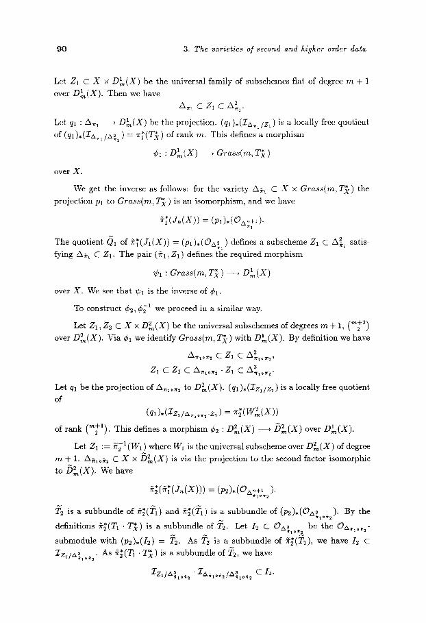
90 3. The varietie~ of ~econd and higher order data
Let Zl C X x D~(X) be the universal family of subschemes fiat of degree m + 1 over DI(X) . Then we have
A,,~ C Z1 C A 2 7r 1 �9
Let ql : Ar t ) Dim(X) be the projection. (ql),(2"/N~/z~ ) is a locally free quotient
of (ql),(ZA~/A~) ---- ~r~'(2r~() of rank m. This defines a morphism
r Dtm(X) > Grass(m,T~ )
over X,
We get the inverse as follows: for the variety A~, C X x Grass(m,T~() the
projection Pl to Grass(m, T}) is an isomorphism, and we have
+l(J.(X)) = (p,).COA_.+,).
The quotient (~1 Of f r~(J l (X)) = (p,),(O/,~) defines a subscheme Zl C A2,~, satis-
fying A ~ C Z1. The pair (~'1, Z1) defines the required morph ism
~i : Grass(m, T~) ~ D I ( x )
over X. We see that r is the inverse of (~l-
To construct r r we proceed in a similar way.
Let Z1, Z2 C X x D2m(X) be the universal subschemes of degrees m + 1, (,,+2)
over D~(X). Via r we identify Grass(m, T~:) with Dim(X). By definition we have
A+,,.-,+o.,.,.2 C Z1 C A ~ ,ri-i o .ri- 2 ,
Z l C Z 2 C A . l o r r 2 �9 Z 1 C A 3 7pl o 1T 2 .
Let ql be the projection of A . . . . ~ to D2m(X). (qa)*(Zz, Iz~ ) is a locally free quotient
of
(ql ).CSz;IA.,..o.:,.Z~ ) = 7r~CW2 ( X) )
of rank (m2+1). This defines a morphism r DZm(X) ----+ D~m(X) over DI(X) .
Let Z1 := ~-1 (W1) where W1 is the universal subscheme over D ~ (X) of degree
m + 1. Aeioe, C X x / 9 ~ ( X ) is via the projection to the second factor isomorphic
t o / ) ~ ( X ) . We have
#~(~-~'(J,~(X))) = (p2)*(OA;+),~).
T2 is a subbundle of ~ ( T 1 ) and #;(T1) is a subbundle of (p2).(OA]10+2). By the
definitions g'~(T1 �9 T~) is a subbundle of T2. Let I2 C OA~10+ 2 be the O/,~1o+ 2-
submodule with (P2).(I2) = T2. As T2 is a subbundle of ~ ( T a ) , we have /2 C
ZZ, IA~to, ,. As ~'~(T1 �9 T~:) is a subbundle of :F2, we have

3.1. The varieties of second order data 91
So we have in particular
Oa~_ �9 12 C 12. ~1 o~-2
3 So 12 is an ideal in O ~ o , 2 , and thus defines a subscheme Z2 C A~o~ 2. By I2 C Iz~/zX~o, ~ we have Z1 C Z2 and by
�9 2 " a . _ , a ~ C 12
we get Z2 C A~o~ 2 �9 Z1. The triple (#lo#2,Z1,Z2) defines the morphism ~2 : b~(X) , D~(X) over r satisfying
* 2 r = (#~r~(J2(X))/T2 = Q2.
Obviously we have ~b2 -1 ---- (~2 �9 U]
In future we want to identify /91(X) with D~(X) and/9~(X) with D~(X) via r and 42.
R e m a r k 3 .1 .8 .
(1) The closure of Z 0,m,(.,2+~) ) (X) in X [(,,:+2)] is
Z(1,m,(,~+~)) (X) = {Z C X[ (m+2)] therewitharexXcE z1X'cZ1z EcZO,m)(X)x �9 Z1 } "
(2) The projection r2 : D2m(X) ~ Z(1,rn,(m:,))(X) is a natural resolution of
�9
y[a] It is the blow up along (3) r2 : D~(X) , y[S] is a natural resolution of "'(a)- --(a) z(1,2)(x).
P r o o f : D~(X) is closed and irreducible. By the d e f i n i t i o n s Z(1,ra,(m+,)) (X) is the
image of the projection r2: D~(X) ~ X [(m~)]. As D2m(X) and Z0,m,(,,+l)) (X)
are smooth, we can easily see that r2 is an isomorphism over the open subset
Z(1,m,(m+l))(X ) o f - Z ( 1 , m , ( m + l ) ) ( X ). r21(Z(1,m,(m+l)))(X ) is dense in D2~(X),
as D2m(X) is irreducible. So Z(,,m,(m2+,))(X) is the closure of Z(1,m,(m+,) ) (X) in
X[(~+2)]. As D2m(X) is smooth, it is a resolution of Z0,m,(,~2+~)) (X). It is easy to
. v[a] is an isomorphism see that "'(3)Y[a] is the closure of Z(1,1,1)(X). r2 : D21(X) ' "'(a)
over Z(1A0)(X ). Z(la)(X) has codimension 2 in y[3] "'(3), as
X [ 3 ] = Z ( 1 , 1 , 1 ) ( X ) I J Z(1,2)(X), (a)

92 3. The varieties of second and higher order data
and Z(1,1,1)(X) is an A d - l - b u n d l e over P ( T } ) and Z ( 1 , 2 ) ( X ) = Grass(2, T~). We
have the exact sequence
o ~ O~ ~ ~ w ? ( x ) ~ r~ - - ~ o.
Let
D~(X)oo := P(T~) C O(W~2(X)) = D~(X).
We see that D{(X)~ is an irreducible divisor in D~(X) and
(D12(X)oo) = r ; l ( z ( 1 , 2 ) ( X ) ) .
(3) follows with the same argument as in the end of the proof of proposition 2.5.8. []
For the rest of section 3.1 let di, el, fi,gi be variables of weight i. Each class
b ~ Ai(X) will also be given weigth i. Let E be a vector bundle of rank r over X.
Then it is well known (cf. e.g. [Fulton(I) ex. 14.6.6]) that we have for the Chow
ring
A*(arass(m, E)) = A*(X)[dl, . . . , d . . . . e l , . . . , em]
djei-j = ci(E), (1 < i < r ,
where we have formally put do = 1,e0 = 1 and dj = 0, e~ = 0 for j > r - m, l > m
respectively. One can summarize these relations to
(1 + dl + . . . + dr-m)(1 + el + . . . "~ ern) = c(E).
One has to note that the relation holds for every weight. We have
e(Tr-m,.) = (1 + dl + . . . + dr-m),
c(0m,E) = (1 + el + . . . + ~m).
In the case of a projective bundle P ( E ) we get in part icular
A*(P(E)) --
where P = cl(Op(E)(1)).
A*(X)[P]
For the Chern classes of a symmetric power of a vector bundle we have the
well-known relation:

3.1. The varieties of second order data 93
R e m a r k 3.1.9. Let E be a vector bundle of rank r over X with total Chern class
c(E) = 1 + el + . . . er. Let c(E) = (1 + Yl) . . . (1 + y~) be a formal splitting of c(E). Then we have
c(Symm(E)) = H ( l + y i , +.. .+Yim). il <.. .<im
If E has rank 2, we have
c(Sym2(E)) = (1 + 2e, + 4e2)(1 + e,)
= 1 + 3el + (2e~ +4e2) H- 4ele2
c(Syma(E)) = (1 + 3el + 9e2)(1 + 3el + 2e~ + e2)
= 1 + 6e~ + (lle~ + 10e:) + (6el + 30e,e:) + lSe~e~ + 94
c(Sym4(E)) = (1 + 2el)(1 + 4e1 + 16e2)(1 + 4e1 + 3el 2 + 4e2)
= 1 + 10el + (35e~ + 20~2/+ (50e~ + 120e,e~)
-t- (24el 4 + 20Sere2 + 64e 2) + 96e31e2 + 128e, e~
c(SymS(E)) = (1 + 5 e I -~- 25e2)(1 + 5e I ~- 4e~ + 9el)(1 + 5 e l -~ 6e~ + e2)
= 1 + 15el + (85e~ + 35e2) + (225e~ + 350ele2)
+ (274el ~ + l lSae% + 2594)
+ (274e~ + 1540e~e2 + 1295ele~) + 600e14e2 + 1450e~e~ + 225e~.
If E has rank 3, we get
c(Sym2(E)) = (1 -F 2el -F 4e2 -{- 8e3)(1 -F 2el + el 2 -t- ele2 - - e3)
= 1 + 4e, + (5~ + 5e~) + (2e? + n e l e : + 7e3)
+ (6e~e: + 44 + 14ele3) + ( S e ~ + 4e14 + ~e:e~)
+ (8ele2e3 -- 8e2).
Definition 3.1.10. Let Yl,... yr be variables and f l , . . - , f r the elementary sym-
metric polynomials in the Yi. Let
c m ( f ' , ' , f ~ ) := 1-I ( l+y~,+.. .y~,o) il <_... <_im
viewed as a polynomial in the fi. Each fi has weight i. Let c m ( f l , . . . , f~) be the
par t of weight i in c m ( f l , . . . , f,.).
From the above we see that for a vector bundle of rank r over X with Chern classes e l , . . . , er the formula
c(Symm(E)) = crn(e, , . . . , e,.)

94 3. The varieties of second and higher order data
holds. In future we don ' t want to distinguish between classes a E A*(X) and
zr;(a) e A*(Dlm(X) and also not between b e A*(DI (X)) and Try(b) e A*(D~(X)).
Proposition 3.1.11.
A*(D2m(X))
A*(X) [dl , . . . , d d - m , e l , . . . , e m , f l , . . . f d - m , g l , . . . , g ( ~ l ) ]
where
d I (1 +dl + . . . + rid-m)(1 + el + . . . + era) = ~ ( - 1 ) ' c i ( X ) ,
(1 q- f l -4-. -4- fd-m)(1 Jr- gl q-.. q- g(~+~))
= ( 1 + d l + . . . + d d - m ) C 2 ( e l , . . . , e m )
c(T,) = (1 + d, + . . . + d~_m),
c(Q1) = (1 + el ~-...-~- era),
c(T2) = (1 + fl + - . . + fd-m),
c(Q2) = (1 q- gl + . . . q- g(.~+l)).
If X is a smooth projective variety over C, the same result holds, if we replace the Chow ring A*(.) by the cohomology ring H*(., 2g) everywhere.
Proof." By the above D~(X) is isomorphic to the Grassmannian bundle
Grass(("+'), W2m( X ) ) over Grass(m, T~ ). The exact sequence
0 - ~ Sym2(Q1) ---* W~(X) ~ T1 ~ 0
gives C(Wm(X)) = c(Sym2Q1)c(T1). The result follows. []
Two cases axe somewhat simpler:
(1) the variety D~_I(X ) of second order data of hypersurfaces on X.
(2) the variety D~(X) of second order data of curves on X.
C o r o l l a r y 3 .1 .12. For a variable P we write
qi(P) := ~-~(-1)Jcj(X)P i-j , 0 < i < d - 1. j<i
Then we have
"i ~, d 1, , , ~ _-- A*(X)[P, Q] (d ) E ( - 1 ) i p d - i c i ( X ) , i=O
(~) ~ _ , (Q - PI ~_, O (~) C?(q~(P),..., q~-~(PI)
i = 0

3.1. The varieties of second order data 95
where P = cl(Op(T~)(1)), q = Cl(Ot(w~_,(X))(1)).
P r o o f : D2d_I(X) is the projective bundle P (W~_I (X) ) over P(T)~), and we have
ci(Qd-l,T~,) = qi(P). Thus the result follows immediately from proposition 3.1.11. [3
C o r o l l a r y 3 .1 .13.
A*(D~(X)) = H*(X)[P, Q]
) i=0
\ i=0 1
where P = e,(Oe(Tx)(1)), Q = c,(Op(wp(x).)(1)).
Proof." This follows immediately from proposition 3.1.11. []
If X is a smooth projective variety over C, then corollaries 3.1.12 and 3.1.13
also hold, if we replace the Chow ring by the cohomology ring.
We will write the above formulas explicitely for X of dimension smaller or
equal to four.
(1) Let X = S be a smooth surface. Then we have
A*(S)[P, Q] A*(D~(S))= (P2+cl (S)P+c2(S) , )
Q2 + (c,(S) - P)Q + 2c2(S)
w h e r e P = Cl(OP(Ts)(1)), q = Cl(Op(w~(s).)(1)).
(2) Let X be a smooth variety of dimension 3. Then we have
A*(D~(X)) = A*(X)[P,Q] p3 + c,(X)p2 + c2(X)P + c3(X), "~
Q3 _~ ( c l ( X ) _ p)Q2 + (c2(X) - c~(X)P - p2)Q + 2c3(X) ) '
w h e r e P = C l ( o p ( ~ x ) ( 1 ) ) , Q = c~(Op(w~(x).)(1)). A*(X)[P,Q]
A*(D2(X) = pa _ c~(X)P: + c2(X)P - c3(X),
(Q + p - cI(X))(Q 2 + 2(P - Cl(X))Q P) (Q ) + 4 (P 2 - ca(X)P + c2(X))

96 3. The varieties of second and higher order data
where P = q(Op(T~)(1)), Q = Cl(Op(w;(x))(1)).
(3) Let X be a smooth variety of dimension 4. Then we have
A*(D~(X)) = A*(X)[P, Q] P4- k - c l ( X ) pa+c 2( X) P2+ca(x )p+c4(X) ' )
0 4 At_ ( e l ( X ) _ p)Qa + (c2(X) - c l (X)P - - p2)o~ ,
q- (ca(X) - c2(X)P - c i (X)P 2 - p3) q_ 2c4(X)
where P = Cl((.QP(Tx)(1)), Q = ca(Op(w~(x).)(1)).
where
with
A.(D2(X) ) = A*(X)[pl, P2,7"1, r2] (R1, R2, R3, R4 ),
R1 :=p~ - 2plpz + p~cl(X) - p2cl(X) + pac2(X) + ca(X),
R2 :=P~p2 - p 2 + plp2ci(X) + p2e2(X) - c 4 ( X ) ,
R3 :=r~ - ar~r~ + ~i + r ~ ( - 2 p l + e l ( X ) ) + ~1~: (4 ; , - 2 c 1 ( X ) )
+ r~(-2plc l (X) + 3p2 + c2(X)) + r2(-3p2 + 2plCl(X) -- c2(X))
-}- rl(PlP2 -- 2plC2(X) -~- 3p2el(X) -}- ca(X))
- 2p22 + 2p2c2(X) - 2pica(X) + 2c4(X),
R4 :=r31r2 - 2rlr 2 + r~r2(-2px + cl(X)) + r~(2pa - cl(X))
+ r~r2(3p2 - 2p, e~(X) + c2(X))
+ r2(pap2 - 2plc2(X) + 3p2q(X) + ca(X)) + 4pac4(X),
c(T~) : (1 + p, + p2),
c(T2) : (1 + rl + ~2).
A*(D2(X))
A*(X)[P,Q] p 4 _ C l ( X ) p 3 ~_ c 2 ( X ) p 2 _ c 3 ( X ) p ~_ e 4 ( X ) ,
( Q _ p ) ( Q 3 _ 2 ( P - q ( X ) ) Q 2 + 4 ( P 2 - c l ( x ) P + c2(X))Q
+ 8 ( P 3 - e 1 ( X ) P 2 + c 2 ( X ) P - c a ( X ) )
�9 (Qa + 2 ( P - c~(X))Q 2 + (p2 _ 2 q ( X ) P + cl(X)2)Q
-- c l ( X ) P 2 -}- c21(X)P -- c l ( X ) c 2 ( X ) -- c 3 ( X ) )
w h e r e P = ca(Op(T~)(1)), Q = Cl(Op(w~(x))(1)).

3.1. The varieties of second order data 97
D2m(X) as t h e v a r i e t y o f s e c o n d o r d e r d a t a o f m - d i m e n s i o n a l subva r i e t i e s
o f X .
We want to see in what respect D2m(X) parametrizes the second order data of
m-dimensional subvarieties of X. First we will more generally consider the I th order
data of germs of smooth subvarieties.
De f in i t i on 3 .1 .14. Let Y be the germ of a smooth subvariety of dimension m at
x �9 X. Let Iv C O x , , be the ideal of Y in Ox,, . The I th order da tum of Y at x is
the subscheme l+l DI, , (Y) := spec(Ox, , / ( Iy + m x , , ) ).
R e m a r k 3 .1 .15. The l th order data of germs of smooth subvarieties of X are the
points of
z (1 , . , , (mt , ) ..... <./_l))(x) c x[<,*')]
(see 2.1.5, 2.1.6, 2.1.7).
P r o o f i For Y C X a smooth subvariety defined in a neighbourhood of x E X we
have
Dt , , (Y) �9 Z(1,,~,(m+l ) ..... (my_l) ) (X) .
Now let Z �9 Z(1 ....... (m+z~_,))(X) and supp(Z) = x �9 X. Let Iz be the ideal of Z
in Ox,, . Then there are local parameters ( X l , . . . , Xd) near x such that
~ l + l IZ = (Xm+l , . . . ,Xd ) -~ " 'X,x"
Let Y C X be the smooth subvariety defined in a neighbourhood of x by the ideal
Iy := (Xm+l, . . . , Xd). Then we have DI, , (Y) = Ox,z / I z . []
Because of remark 3.1.15 we write
#m(X)o := Z(1 ....... (m+/_l))(X).
We see that D~(X)o = y[n+l] (see remark 2.1.8). So D~(X)o parametrizes ~(n+l),c I th order data of smooth m-dimensional subvarieties of X. It is easy to see that
Dlm(X)o -= Grass(m,7~(). For 1 _> 2 and d _> 2 however D ~ ( X ) is not compact.
R e m a r k 3 .1 .16. Let Pl : Dlm(X)o , l-1 D m (X)o
DI, , (Y) , , D t - I , , ( Y )
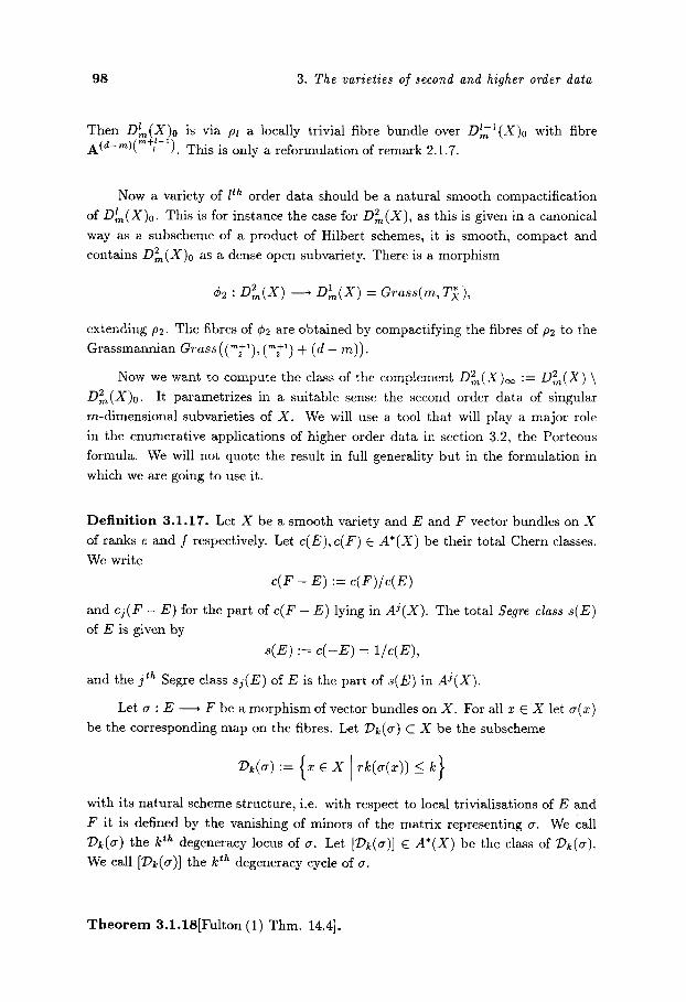
98 3. The varieties of second and higher order data
Then DIm(X)o is via Pt a locally trivial fibre bundle o v e r D~-l(X)0 with fibre
A(d-m)(m+t-1). This is only a reformulation of remark 2.1.7.
Now a variety of I th order data should be a natural smooth compactification
of D~(X)o. This is for instance the case for D~(X), as this is given in a canonical
way as a subscheme of a product of Hilbert schemes, it is smooth, compact and
contains D2m(X)o as a dense open subvariety. There is a morphism
r D~m(X) ~ Dim(X) = Crass(m,7~ ),
extending P2- The fibres of r are obtained by compactifying the fibres of p2 to the
Grassmannian Grass(("+'), (,~+1) + ( d - m)).
Now we want to compute the class of the complement D~(X)oo := D~(X) \ D~(X)o. It parametrizes in a suitable sense the second order data of singular
m-dimensional subvarieties of X. We will use a tool that will play a major role
in the enumerative applications of higher order data in section 3.2, the Porteous
formula. We will not quote the result in full generality but in the formulation in
which we are going to use it.
D e f i n i t i o n 3 .1 .17. Let X be a smooth variety and E and F vector bundles on X
of ranks e and f respectively. Let c(E), c(F) E A*(X) be their total Chern classes.
We write
c(F - E):= c(F)/c(E)
and ci(F - E) for the part of c(F - E) lying in AJ(X). The total Segre class s(E) of E is given by
4 E ) := c ( - E ) = 1/4E),
and the jth Segre class s / (E) of E is the part of s(E) in AJ(X).
Let a : E -----* F be a morphism of vector bundles on X. For all x r X let a(x) be the corresponding map on the fibres. Let :Dk(cr) C X be the subscheme
with its natural scheme structure, i.e. with respect to local trivialisations of E and
F it is defined by the vanishing of minors of the matrix representing a. We call
~k (a ) the k th degeneracy locus of a. Let [~Pk(a)] r A*(X) be the class of ~Pk(a).
We call [T)k(a)] the k th degeneracy cycle of a.
T h e o r e m 3.1.18[Fulton (1) Thm. 14.4].

3.1. The varieties of second order data 99
(1) Each irreducible component of :Dk(rf) has codimension at most r := ( e - k ) ( f - k) i n X .
(2) If the codimension of T)k(a) in X is r, then we have:
[:/)k(a)] ---- dct ( (c f -k+i- j (F - E))l<_i,j<_e-k).
We consider the morph ism
r 7r~(Sym2(Q1)) ---+ Q2
of vector bundles on D ~ ( X ) which is defined by the d iagram
0
1 T2
1 0 , ~r~(Sym2(Q1)) ~ W ~ ( X ) , T1 ~ 0
Q2
l 0.
Then D ~ ( X ) ~ is the degeneracy cycle
l?(mr162 := {v e D ~ ( X ) r not onto }.
The intersection of each fibre 7r~-l(v) with D2m(X)~ is a divisor in rr~-l(v). So we
get by the Porteous formula:
[ D ~ ( X ) ~ ] -- c1(Q2) - ~r~(cl(Sym2(Q1)))
= c1(Q2) - (rn + l)Tr~(cl(Q1)).
R e m a r k 3 .1 .19 . Let Y C X be a smooth locally closed subvariety of dimension
m0 >_ m. Then D2m(y) is in a natural way a locally closed subvariety of D 2 ( X ) . If
Y has dimension rn, then D2m(Y) is isomorphic to Y in a na tura l way.
Definition 3.1 .20. Let Y1,Y2 C X be smooth locally closed subschemes of di-
mensions dl, d2 > rn and x C X. We say Y1, Y2 have I th order contact along an

100 3. The varieties of second and higher order data
m-dimensional subvariety at x, if x C Y1 A Y2, and there is a germ of a smooth
subvariety Z C X at x satisfying Dl,x(Z) C Y~ and Do:(Z ) C Y2.
We say Y1, II2 have m-dimensional l th order contact, if there is an x C X such
that they have I th order contact along an m-dimensional subvariety at x. If m is
the min imum rain(d1, d2), we say in this case that Y1 and Y2 have l th order contact
(at ~).
From the definitions we get immediately:
R e m a r k 3 .1 .21. Y1 and Y2 have m-dimensional I th order contact at x, if and only
if D~(Y1)o, and D~(Y2)o intersect as subvarieties of Dtm(X)o in points lying over
x E X .
In case dl = m <_ d2, Yt and Y2 have second order contact at x if and only if
D2m(Y1) and D~(Y2)intersect as subvarieties of D2~(X) in points lying over x E X.
(In this case the intersection point automatically lies in D2~(Y1)o N D2m(Y2)o, as Y1
is smooth of dimension m, and D~(X)o A D2m(Y2) = D~(Y2)0.)

101
3.2. Varieties of higher order data and applications
We now want to t ry to generalize the definition of the varieties of second order
da t a to a definition of varieties of higher order data . We will however only have
par t ia l success. This means tha t we give a general definition of the variety D ~ (X) of
n th order da t a of m-dimensional subvarieties of a smooth variety X, which however
does not behave very well in general. The varieties of th i rd order da t a of curves
and hypersurfaces on a smooth variety X turn out to be project ive bundles over the
corresponding varieties of second order data . However the varieties of th i rd order
da t a of subvarieties which have bo th dimension and codimension greater or equal
to two are not locally tr ivial fibre bundles over the corresponding varieties of second
order data. Also, even if X is a surface, D~(X) is not a locally tr ivial fibre bundle
over D~(X). At the end of this section we give some enumerat ive appl icat ions of
our results.
As a s t ra ightforward general isat ion of the definition of the varieties of second
order da t a of m-dimensionM subvarieties of a smooth variety X we get the following
definition:
D e f i n i t i o n 3 .2 .1 . Let X be a smooth project ive variety of dimension d over a field
k. Let n,m E 2~>_o with 1 < m < d. Let ~),~(X) be the contravar iant functor from
the category of noether ian k-schemes to the category of sets which for noether ian
k-schemes S, T and a morphism r : S ~ T is given by:
I)~(X)(T) : { (Zo,..., Z,~)
Zi C X x T closed subscheme flat of degree (re+i) over T (i = O , . . . , n ) } Zo C Z1 C . , . C Zn
and Zi " Zj D Zi+j+l for all i,j with i + j < n - 1
p~,(x)(r : ~ ( X ) ( T ) , ~ ( X ) ( S )
( Z o , . . . , Z n ) , , ( Z o •
Here we use again the notat ions we have in t roduced in definition 3.1.1. In the same
way as in l emma 3.1.2 we can show tha t : / )n(X) is represented by a closed subscheme
D ~ , ( X ) c X x XEm+,1 x . . . x X [(into)].
We call D~(X) the variety of n th order da t a of m-dimensional subvarieties of X.
D~(X) is as a subset o f X [m+l] x . . . x X [ ( '~"+n)] given by:
( z 0 . . . . . z n ) c D~m(X) :=
x • xEm+, l • • x [(~:")]
Z0 C Zl C Z2 C . . . C Zn / and Zi - Zj D Z i+ j+ l /
for all i,j with i + 3 _< n - 1

102 3. The varieties of second and higher order data
Obviously we have D~ = X. For i = 0 , . . . , n let
r i : D~(X) ~ X [(~'+')]
be the project ion. We also consider the projec t ion
~r. : D~(X) , Dnm-I(x)�9
It is not clear in which cases D,~(X) is reduced, i r reduble or smooth. In
cases in which it is reducible a be t te r candida t for the variety of higher order
d a t a is the closure the image of D~(X)o under the obvious embedding. Let
A C X x X be the diagonal. Then Hilb('+m)(Ai+l/X) is a closed subscheme
of Hi lb( '+m)((X x X ) / X ) = X[( '+m)] for all i. We can see immedia te ly tha t the
projec t ion ri: D~(X) ~ X [ ( '+ ' ) ] factors through Hilb('+~)(Ai+I/X), as we see
from the definitions tha t Hilb('+'~)(Ai+~/X) represents the functor
T I , {(Zo, zd Z0, Zi C X • T closed subschemes )
fiat of degrees 1, (re+i) over T /
Zi C Zg "}-1
We now want to show tha t D~(X) and D3d_a(X) are again Grassmannian
bundles corresponding to vector bundles over D~(X) and D ~ _ I ( X ) respectively.
Before doing this we want to show tha t these two cases are the only ones in which
we can expect such a result (exept for the t r ivial case m = d).
R e m a r k 3.2.2.
(1) Let 2 < m _< d - 2. Then ~r3 : DO(X ) ~ D~(X) is not a locally t r ivial fibre
bundle�9
(2) Let S be a smooth surface. Then 7r4 : D4(S) , D~(S) is not a locally tr ivial
fibre bundle.
Proof.* (1) Let x E X. Let xa . . . . Xd be local pa ramete r s near x and let
mx,~ := (xl . . . . ,xa)
be the maximal ideal at x. Let Z1, Z2 be the subschemes of X with suppor t x
defined by the ideals I1 = (xm+l,.. ,xd) T m 2
�9 Xp~g~
I2----(Xm+l, . , X d ) T m 3 �9 �9 X ~ x

3.2. Varieties of higher order data and applications 103
in Ox,, . Then we have (x, Z1,Z2) E D~(X) . The fibre rc31((x,Z,,Z2)) consists
exactly of the subschemes Z3 C X with support x whose idea l /3 in Ox, , is of the
form
I3 = ( V ) -[- (Xm.t- 1 Xd)" m x , . + m 4
for some (d - m)-dimensional linear subspace V of
(Xm+l ...Xd> -t- <XiXjXl [ i , j , l <_ m).
(Here we denote by ( f l , . . . , f~) the span as a vector space in contrast to ( f l , . . . , h ) ,
which denotes the ideal generated by the fi.) So we have
~ ; ' ( ( x , Zl , z2)) "~ a r a ~ ( ( " ? ) , d - m + ( '22) ) .
Let Z~ C X be the subscheme with support x defined by the ideal
1 ; : = ( X m - 4 - 3 , . . Xd,X2,XlX2)-~-(XiXj[i > m ) + m 3 �9 ~ X,x
in Ox,, . Then (z, Z1, Z~) i s a point of D~(X) . The fibre rr31((x, Z1, Z~)) consists
of exactly those subschemes Z~ with support x whose ideal I~ in Ox, , is of the form
/~ =(w) + ( z~z j l i >_ m + 3) + ( x~x i l i , j > m + 1) + ( x ~ z i , X l ~ i < d)
+ ( ~ z ~ x , l i > m + 1) + m~x,.
for an (m+2)-codimensional linear subspace W of
V := <Zrn-t-3,... ,Xd, X2,XlX2> 2[_ <Xm+lXi,Xm.l_2Xi li < m>
+ (xixjxz[1 < i < j < l < m; j > 2>.
By dim(U) = d - m + (,,,+2) + 1 we have
% ' ( ( z , Z , , Z ' ~ ) ) ~- Grass((~+2),d - m + 1 + (~+~)).
(2) Now let S be a smooth surface, s E S and x, y local parameters near s. Let
Z1, Z2, Z3 be the subschemes of S with support s defined by
I1 :-- (x, y2),
I2 := (~ ,y~) ,
13 := (x,y4).
Then we have (s, Z1, Z2, Za) e D3(X). Thus r~-l((s, Z1, Z2, Za)) consists of the
subschemes Z4 with support s whose ideal /4 in Os, s is of the form /4 = w + (x 2 , xy, yh) for a one-dimensional linear subspace w C (z, y4 ). So we have
7r41 ((s, Z l , Z2, Z3)) ~-~ P1.
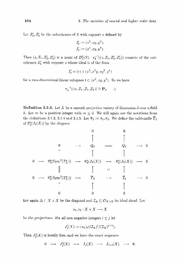
104 3. The varieties of second and higher order data
Let Z~, Z~ be the subschemes of S with suppor t s defined by
I ; := (x2 ,xy ,y2) ,
/~ := (x2,xy, y3).
Then (s, Z1, Z~, Z~) is a point of D~(S). zr4~((s, Z1, Z~, Z~)) consists of the sub-
schemes Z~ with suppor t s whose ideal is of the form
I'~ = (t) + ( x ~ , ~ > x y ~ , ~ ~)
for a two-dimensional l inear subspace t C (x 2, xy, y3>. So we have
7F41((W, Zl ,Z2, Z3)) ~ P2. []
D e f i n i t i o n 3 .2 .3 . Let X be a smooth project ive variety of dimension d over a field
k. Let m be a posit ive integer with m < d. We will again use the nota t ions from
the definitions 3.1.3, 3.1.4 and 3.1.5. Let ~2 := #loft2. We define the subbundle T2
of ~ ( J a ( X ) ) by the d iagram
0 0
T T 0 ' Q2 Q2 ~ o
T T l 0 ---+ ~ ( S y m a ( T ~ ) ) ~ ~-;(da(X)) - -~ ~ ( J : ( X ) ) ) 0
0 - - ~ ~ ( S y m a ( T ~ ) ) ~ T2 - - ~ T2 , 0
T T T 0 0 0
Let again A C X x X be the diagonal and Zt, C O x x x its ideal sheaf. Let
sl ,s2 : X x X ----* X
be the projections. For all non-negat ive integers i _< j let
J j ( X ) := (S2) . ( (Za) i / ( zA )J+I).
Then J~(X) is locally free, and we have the exact sequence
0 , J~(X) - -* J j ( X ) - - + J i -~ (X) , O.

3�9 Varieties of higher order data and applications 105
We see J~ = Jj(X) and Jj(X) = SymJ(T~). Let il <_ i2 < j2 _< j l be positive
integers�9 The multiplication in Ox • gives a morphism
�9 : (z~)~I/(zA)Jl | (ZA)'~/(ZA) j2 ---* (ZA)~I+~=/(Z,,)i'+J~
of sheaves on X • X. So it gives a morphism of locally free sheaves
�9 4 : ( x ) | 4 : ( x ) __~ ~+,2 : Ji~+j2 (X).
For locally free subsheaves F C J;:(X), G C J]:(X) we denote by F . G the image
of F | G under ".". This is a coherent subsheaf of Jit+i2{x]il+j2 ~ j. By definitions 3.1.4
and 3.1.5 we have
W2m(X) = T1/(T1. # ; ( ~ ) ) ,
and T2 is a subbundle of #~(W2~(X)). T2 is the preimage of
T2 C 7r~(W2m(X)) C -~(J2(X))/(~;(T1)" V~(T~))
under the natural morphism
p : W~(Ja(X)) , ~(J2(X)) / (~(TA).~(~I~)) = ~ ( J 3 ( X ) ) / ( ~ i ( r l ) - * 1 �9 ~ (J~ (x))) .
Here for coherent sheaves F, G we write F C G to mean that F is a subsheaf of G.
So ~r~(T1).-~(J~(X)) is a subbundle of T2, and we have
T - 2 / ( ~ ' ; ( T 1 ) " ~;(Jl (X))) = T2.
From T2 C ~r~(T1) C ~'~(J~(X)) we get
r ~ 2 - - * 1 ~ . �9 7r2(J2(X)) C ~;(T1) V;(J~(X)), ~ ~ * ~ --* 1 --* 1 +~(T1)" +~(T1) C rr2 (T1) �9 u2(J2(X)) C T2 C u2(Ja (X)).
a a b2~(X) by We define the coherent sheaves Uam, V~, W~m(X) on
u~ : = ( ~ ( ~ ) - * 1 ~* �9 71"2(,]2 ( X ) ) ) / ( T r 2 ( T i ) " ~ ' ; (5~1)),
7 3 : = ( # ; ( r l ) " 7c2(J~(X)))/(Tr2(T~)" 9~(T1) + T2 .~(J~(X))) ,
w ~ ( x ) : = ( T ~ ) / ( ~ ( ~ ) . #~(~) + (:~). ~ ( j l ( x ) ) ) .
Then we obviously have the exact sequence
o , v ~ ~ w s ~ T~ - - - , O.
L e m m a 3 .2 .4 . L e t m = 1 o r m = d - 1.

106 3. The varieties of second and higher order data
m+2 (1) U3m is locally free of rank r e ( d - m) -[- ( 3 )"
(2) Vain i~ locally free of rank (m+2] 3 / "
(3) W~m(X) is locally free of rank e - m + (m+~ 9"
P r o o f : By the exac t sequence
o , v ~ , w ~ ( x ) , T~ , 0
it is enough to show these resul ts for [/am and V~. It is enough to check t h e m
fibrewise. Let v 6 D ~ ( X ) be a poin t lying over x 6 X . Let x l , . . . , X d be local
p a r a m e t e r s near x. For i = 1 . . . . , d we denote by ~'i the class of xi in Ox ,~ /m~: ,~ .
We can as sume tha t the fibre ~;(Tl (v) ) is of the fo rm (Xm+l, . . . ,Xd)/m2x,x. T h e n
we have for the fibres:
( ~ 1 . . . . 1 �9 ~r2~r2J ~ ( x ) ) ( v ) = <~22j[i > m ) + ( '2 i~jx t[ i , j , l <_ d),
(e~(T~) e~(T1))(~) : <~,~ l i , j > .~> + <~{~j~, li > - J .
Let A0 : : (~iYcj I i < m , j > rn} + (Yzi~j2z [ i , j , l < m). T h e n the res t r ic t ion of the
na tu r a l p ro jec t ion
~ : ( ~ T I ~ J ~ ( x ) ) ( ~ ) , V ~ ( v )
to A0 is an i somorph i sm, and (1) follows.
T2(v) is an (m - d ) -d imens iona l l inear subspace of
~ ( w ~ , ( z ) ) ( v ) - * - . . . . . = (7c2T,/(rc2T, �9 7r2T}))(v ).
Let p : f r~(W~(X)) (v ) ~ fr~(T1)(v) be the pro jec t ion . As we have a s sumed tha t
rn = 1 or m = d - 1 holds, we have e i ther p(T2(v)) = ~r~(T1)(v), or p(T2(v)) has
cod imens ion 1 in ~r~(T~)(v). (~~(T1)(v) is one -d imens iona l in case m = d - 1, and
T2(v) has cod imens ion 1 in ~r~(W~(X))(v) in case m = 1.)
(a) p is onto. T h e n we have
f~(v) (ym+~,.. 3 = . , y d ) / m x , ~ ,
where x l , �9 �9 Xm, Y m + l , . - �9 , Yd are local p a r a m e t e r s near x. So we can as sume
tha t xi = yi for i = m + 1 , . . . , d . T h e n we have
(~. ~;(J~(x)))(v) : <},~ li > ~)+ <~,~j~ li > ~).
Let A1 := (~2i2.j24[i,j, 1 <_ m). T h e n the res t r ic t ion of the na tu r a l p ro j ec t i on
ql : (~r~(Tx). ~ ( J ~ ( X ) ) ) ( v ) , V3m(V)

3.2. Varieties of higher order data and application~ 107
to A, is an isomorphism, and (2) follows.
(b) p(T2(v)) has codimension 1. By changing the local coordinates if neccessary
we can assume
T2(v) = ((Xm+2,. . . ,Xd, f ) + ( X m + l X j [ j < _ ' m + l ) ) / m x , x 3
for an f C (xixj l i , j < rn) \ m 3 Let f denote the class of f in Ox,x/m4x,~. - - X ~ : c "
Then we have
(T2" ~;J~(X) )(v) = (.~ixj ]j >_ m + 2) + (x, ix, j~,l [ i > m) + ( f 2t ] l <_ m).
Let A2 := (2~m+l~i [i <_ m) + (~iY:j~tli,j, l < m). Then the restriction of the
natural projection
q2 : ( #~ (T , ) ' ~(J~(X)) ) (v ) --~ V2(v )
to A~ is a surjection with kernel (f2~ [i _< rn), and (2) follows. []
Def in i t ion 3 .2 .5 . We put
/)la(X) := P(W~(X)) = P((Wla(X))*) ,
/ ~ _ , ( X ) := P ( W ~ _ , ( X ) ) = I~((W~_,(X))*).
For m = 1 or m = d - 1 let ha : ba~(X) ~ b2m(X) be the projection and
~a := hi oh2og'a. Let Ta := Td-m,wam(X ) be the tautological subbundle and
ia 0 -----+ T3 ~ h;(W3m(X)) _2~ Q3 ---, 0
the canonical exact sequence. Let
It" := h ; ( T 1 ) ' h ; (T , ) + T~. V;(ZJ (X))
be the kernel of the natural vector bundle morphism ~ : T2 - - ~ W~(X) . We define
the vector bundle T3 o n / ~ ( X ) by the diagram
0 , T3
T 0 ,
T 0 - - - , h ; ( K )
T 0
i 3
[3
~
i3 )
0 0
T 1
?r~(T2) ~ Qa
T T - ~ ; ( K ) , 0
T 0
, 0
, 0

108 3. The varieties of second and higher order data
and the vector bundle 03 o n / ) a ( X ) by
0 0 0
0 ----+ T3 is - - 4~ - -~ #~(T2) ' Q3 - - ~ 0
l 0 ~ eft 3 "--')" ~:~(J3 ( X ) ) ~ (~3 ;' 0
773 (Q2) ' 0
0 0
In part icular we get the exact sequence
0 ~ 03 )3 # 3 03 ~ . -- ' ' z(QJ) ----* 0.
We now generalize the definition of the bundles (Ox)~ and (Ox)2~ from 3.1.3:
D e f i n i t i o n 3.2.6. For any I C /V let again Zt(X) C X x X[q be the universal
subscheme with the projections
z~(x) / p , \ q ,
X X[O.
For any vector bundle E of rank r on X we put
/~t := (qt).(p~(E)).
This is a vector bundle of rank rl on X [z]. For all n E ~W and all m _< d we put
(E)~ := rn(E(,,+,)),
where r,~ : D~(X) ~ Z[(~+n)] is the projection from 3.2.1. ( E ) ~ is a vector
bundle of rank r . (m+,~) on D~(X). We call it the contact bundle corresponding to
E,X and m.
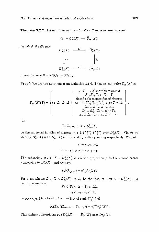
3.2. Varietie, of higher order data and applications 109
T h e o r e m 3.2 .7 . Let m = 1 or m = d - 1. Then there is an isomorphiam
< := D~m(X) --~ b~m(x),
for which the diagram Dam(X) r , Dam(X)
Dam(X) r , s
commute, such that r = (Ox)am.
Proof." We use the' nota t ions from definition 3.1.6. Then we can write 1)am(X) as
Let
1)~(X)(T) = { (r Z1, a2, Z3)
r : T ~ X morphism over k Z1, Z2, Z3 C X x T / closed subschemes flat of degrees
rn + 1, (m+2), (m+3) over T with .
Aq5 C Zl C Z2 C Z3, Z1 C A~, Z 2 C Ar �9 Z1,
Za c A r Z a c Z ~ - Z 1 .
Z1, Z2, Z3 C X x Dam(X)
(re+z) (m+3"~ Dam(X). Via r we be the universal families of degrees m + 1, t 2 J, ~ a J over
identify/gzm(X ) with Dam(X) and #1 and #2 with rrl and 7r2 respectively. We put
71" ;~ 7rloTr2o7r3~
# := #1o#2o#3 = 71-1o7r2o# 3,
The subvariety A,~ C X x Dam(X) is via the projec t ion p to the second factor
isomorphic to Dam(X), and we have
p . ( Q : + , ) : ~*(&(x)). For a subscheme Z C X x D a ( x ) let Zz be the ideal of Z in X x Dam(X). By
definition we have Z2 C Z a C A ~ . Z 2 c A 4,
Z3 C Zl �9 ZI C /N4.
So p,(Zz2/za) is a locally free quotient of rank (m+2) of 3
p,(Zz~/(za. .z~ + Zz,.z, )) = ~ ( w ~ ( x ) ) .
This defines a morph i sm Ca : D 3 ( X ) ~ D 3 ( X ) over D2(X) .
110 3. The varieties of second and higher order data
Let Za := ga l (W~) , Z2 := ~-31(W2) for the universal subschemes W1 and W2 over D2m(X) of degrees m + 1 and (m+2) respectively. The subvariety Ae C
X x/gam(X ) is via the projection i5 to the second factor isomorphic t o / ? a ( X ) , and
we have
~ , ( o ~ ; + , ) = ~*(J,(x)).
T3 is an Ob~(x ) - submodu le of #*(J4(X)) . Let Ia C Ozx~ be the Ozx~-submodule
with/5.(I3) = Ta. By the inclusions
rta(rr2(T1))" -* * - ra , ~ ( . : ( T , ) ) c
(see definition 3.2.5) we have
:r/,~lA~ �9 :rZ~lA, C Ia, $ 2
Z, la~ C Ia,
So we have in part icular OA~ - Ia = ira. So Ia is an ideal in Oz~ and defines a
subscheme Za C A 4 satisfying
By the inclusions :I~,,l/, ~ "TUZ~IAI c I3,
I~, l , , ~ c h, Ia c ~Z=la~
we have Z2 c Za c A~. Z2,
Z3 C Z1 " Z1,
Z2 C Za.
(~, Zl, Z2, Z3) defines a morphism ~b3 : Dam(X) - - + D~(X) over D2m(X) satisfying
r = Qa. It is easy to see that r = r []
In future we want to identify Da(X) with /?la(X) and also Da l(X) with bLI(x) .
As D~(X) is smooth, we see first that the projection ra : D~(X) ~ X [4]
factors through y[4] As also X [4] "'(4)" (4),c = Z(1,1,1,1)(X) is smooth, ra is an isomor- phism over Z(1,1,1,1)(X ). The preimage D~(X)o parametr izes third order da ta of

3.2. Varieties of higher order data and applications 111
(germs of) smooth curves on X. Here the n th order d a t u m of a smooth subvariety
O ~m ~+1 of Ox,x . In a s imilar way Y C X in a point x C Y is the quotient Y,x/ x,~
one can t rea t D~_I (X) : the preimage r ~ l ( z ( 1 d-1 (~ ( ~ + ~ ( Z ) ) is an open dense \ ' ' k2 / ' \ 3 ] l
subset Dad_l(X)o in D~_I (X) , and the res t r ic t ion r3[D~_~(X)o is an isomorphism.
r31 (D~_ l(x)0 ) parametr izes th i rd order da t a of (germs of) smooth hypersurfaces
of X.
R e m a r k 3 .2 .8 . Let Y C X be a smooth closed subvariety, Then for all n E ZW the
Hilbert scheme y b ] is a closed subscheme of X b ] . So for all n, m E ZW with m _< d
D ~ ( Y ) is a closed subscheme of D ~ ( X ) . From the definitions of the vector bundles
( O x ) ~ and ( O y ) n we see that (Ox)nlD,~(y) = (Oy) n. So/~2 ( y ) C / 9 ~ ( X ) and
/9~(Y) C / ) l a ( X ) are closed subvarieties with
Q,i(x)[y = Q.i(Y), Q i (X) ]v = Qi (Y) , (i = 1,2,3) .
Here we write Qi(X) , Q i ( X ) for the classes Qi, Qi on D i ( X ) and similar for Y.
In case m = d = d i m ( X ) we see immedia te ly tha t D ~ ( X ) is isomorphic to X
via its project ion. The universal families are Zi = A i+1 C X x X for i = 0 , . . . , n.
So we have (Ox )~ = Zn(X) ,
n n + l ( O X ) m / ( O x ) ~ = Sym"(T~) .
Now we can compute the Chow rings of D ~ ( X ) and D3_I (X) . For this we first
have to determine the Chern classes of WI (X) and wL (x).
L e m m a 3 .2 .9 .
(1) In case m = 1 we have V~ ~ ~r~(Q1) | Q2, and so there is an exact sequence
0 ---* ~r~(Q1)| - - * W3t(X) , T2 --+ 0
on
(2) In case m = d - 1 there are exact sequences
0 ---+ T2| , V#_ 1
o - - ,
0 ----* Vda_l
on 5 L I ( X ).
~ Yd3_l
---+ U~_ 1 ~ f f~(T1) |
---4" W ~ _ I ( X ) ----4 r 2 ) 0

112 3. The varieties of second and higher order data
Proof :
(~) Let ~ : ~ ; (~ ) ~ ~ ( : J ( X ) ) --~ V? be the ~atural homomorphism. We see immedia te ly tha t w is onto and
~; ( J I (X ) ) @ T2 -[- ~ 2 ( r l ) @ 7r2 (T1)
lies in the kernel of w. As all the sheaves we are considering are locally free and
have the right rank, we have
and obviously this is also the kernel of the na tu ra l map w : 9i( :F1) | ff~(j1 (X)) - - ~
# i ( Q i ) | Q: .
(2) We a l ready know the lower sequence. The middle sequence comes from the
d iagram
0 0 0
l 1 1 0 ~ ~ ; ( T 1 ) . ~ ( J ~ ( X ) ) ~ ~'~ ( r l ) "~'~ ('~1) ~ ~r~ (Sym2 (T1))
0 ~ ~ ( S y m a ( r ~ ) ) ~ ~r~ ( ' ~ 1 ) - ~ ( J1 ( X ) ) ~ ~-~ ( r l ) . ~ ( T ~ )
0 ~ ~r~ ( S y m a ( Q 1 ) ) - - U~_ 1 ~ (~r~ (T1 ) .~ (T~) ) /Sym~( f r~ (T~) )
0 0 0
if we use (T1 �9 #~(T~i))/Sym2(T1) ~= T1 | Q1.
Let w2 : U~_ 1 ) V)_ 1 be the na tu ra l homomorphism. ex~ ~ . ker(w2) = T2 | % (QI). We consider the exact sequence
~2+~(jl(X)) ~ uL~ - ~ v)_~
We have to show
O,
where w0 is the obvious map. We see tha t
(~';(T1) % ( T ~ ) ) - * 1 ~ ' ~ ( r l ] r 1 6 2 �9 - * * Q ~ ( J ~ ( z ) ) + ~ e ) c
and (T~| (X)))/((~;(T~). ,~(T~)) 0 ~ ( j I ( x ) ) + ~ 0 ~ ; (~) )
~- ~ | ~(T:,.)/((~;(T~). ~(T~)) 0 ~;(T~) + ~ 0 ~(T~))
~- T2 | ~;(O,). So there is a surjection of vector bundles

3.2. Varieties of higher order data and applications 113
Because the bundles have the same rank, it is an isomorphism. So (2) follows. []
Again for i = 1,2, 3 we don't want to distinguish notationally between a0 in
A*(Di - ' (X) ) and ~r~'(ao). We formulate our results (proposition 3.2.10 and propo-
sition 3.2.11) only for the Chow rings, but it is clear that they also hold if we replace
the Chow rings by the eohomology rings everywhere.
P r o p o s i t i o n 3.2.10. Let X be a smooth projective variety of dimension d. Then
A*(D~(X)) = A*(X)[P, Q, R] d
Z Pd-ici(X), i = 0
• ci(X) - 2c i - l (X)P - E cj(X) i = 0 j=O
pQi-l-j i - -2-- j '_ '_ x
Here P = C l ( O P ( T x ) ( 1 ) ) , Q = C l ( O p ( w ~ ( x ) . ) ( 1 ) ) , R = c l ( O p ( w a ( x ) . ) ( 1 ) ) .
Proo f : This follows immediately from lemma 3.2.9(1). []
P r o p o s i t i o n 3.2.11. Let X be a smooth projective variety of dimension d. As an abbreviation we write qi(P) := ~j<_i(-1)Jcj(X)P i- j , 0 < i < d - 1. Then we
have with the notations of definition 3.1.10 and corollary 3.1.12
�9 a A*(X)[P, Q, R] A (Dd_a(X))=
d
Z ( - 1 ) i p " - i c i ( X ) , i = 0
(Q - P) qd-l(P)), i=O
(R-e ) E / = 0 n = O
\ i+ j<d-1 qi(P) j
- - / - - T t

114 3. The varictie~ of second and higher order data
tlere (.),, de~ote~ the part of degrer ,~ (P,Q,R have each degree 1 and ci(X) ha~ d~gree i). We have P = ~ ( O p ( r ~ ) ( 1 ) ) , Q = c~(Op(wL, (x ) ) (1 ) ) , n =
cl(Op(w2_,(x))(1)).
P r o o f i By the exact sequences from lemma 3.2.9(2) we get
e ( W 3 _ I ( X ) ) c 3 - , c #* -* = ( S y m (Tc:(Q~))) ( 2(Q1)Q~r~(T1))c(T2)/c(T2 |
and for a vector bundle E of rank r and a line bundle A we have
( r - i ) c i ( E ) c l ( A ) J . [] e(E | A) = ~ j i+j=r
We will rewri te these formulas explici tely for d < 3.
If X is a surface, then
A*(X)[P, Q, R] A*(D~(X)) = p2 + Cl(X)P + c2(X),
Q2 + (c~(X) - P)Q + 2c2(X), ] ,
] R 2 + (c~(X) - 2P)R + c~(X) - 2c~(X)P - PQ
If d = d im(X) = 3, then
A*(X)[P, Q, R] A*(Ds(X)) = liPS + c l (X)p2 + c2(X)P + cs(X),
L Qa + (Cl(X) _ p)Q2 + (e2(X) - c~(X)P - p2)Q + 2ca(X),
R 3 + ( c l ( X ) - 2 P ) R 2 + (c2(X) - 2Cl(X)P - P Q ) R
+ ca(X) - 2c2(X)P - c l ( X ) P Q - p(Q2 _ pQ).
�9 and
where
A*(Ds(X)) = A*(X)[P, Q, R]
(Sl , $2, $3)
Sx : : P ~ - e ~ ( x ) P ~ + e : ( X ) P -- c~(X),
$2 : = ( Q - P)(Q + P - cl(X))(Q 2 + 2 ( P - c~(X))Q
+ 4 ( P 2 - cl(X)P + c2(X)),
$3 :=R 5 + (4P + Q - 6c l (X) )R 4 + (12P 2 + 2PQ - 23Pe1(X)
+ Q2 _ 3Qcl(X) + 11e 2 + 10c2)R 3

3.2. Varieties of higher order data and applications 115
+ (4p2Q _ 35p2cl(X) _ pQ2 _ 2PQcl(X) + P(41c,(X): + 23c~(X))
q_ Q3 + 2Q2cl(X) + Q(_4Cl(X)2 + 8c2(X)) - 6c l (X) 3
- 30cl(X)c2(X) + l lc3(X))R 2
+ (_p2Q2 + 9p2Qci(X) + p2(24c1(X)2 + 15c2(X)) - 3PQ 3
+ 14PQ2cl(X) + pQ(-21c~(X) 2 - 25c2(X)) + P(-24c~(X) 3
- 57cl(X)c2(X) + 6c3(X)) -I- 6Q3cl(X) q- Q2(-18cl(X)2 q- 9c2(X))
+ Q(12c~(X) 3 + 3cl(X)c2(X) - 13c3(X)))n
- - 21p2Q 3 + 99p2Q2cl(X) + P2Q(-66c1(X)2 - 19c2(X))
"4- P2(-168Cl(X)c2(X) -4- 56c3(X)) -4- 75pQ3 c1(X)
+ PQ2(-137ci(X)2 - 126c2(X)) + PQ(66cl ( x ) 3 + 99cl(X)c2(X) + 6c3(X))
-4- Q3(-68ci(X)2 + 5c2(X)) -4- Q2(36cl(X)3 + 111c1(X)c2(X) - 54c3(X)).
Let E be a vector bundle of rank r on a smooth project ive variety X. Now
we want to s tudy the vector bundles (E),~ from definit ion 3.2.6. For this purpose
we first consider the bundles /~t on the Hilbert scheme X Ill. We can associate in a
na tu ra l way to each section s of E a section ~) of fist and thus also a section (s)" m of
(E)7.:
D e f i n i t i o n 3 .2 .12 . For any point Z E XM the fibre /~t(Z) of fist over Z is the
vector space H~ E | Oz). Let
evz : H~ ~ H~ | Oz)
be the evaluat ion morphism. For any section s E H ~ E) we define a section ~t of
fist by
~ t ( z ) := ~vz(s)
and put ( s )~ := r*(s~(,~+,)). This defines the evaluat ion morphism
eVE: H~ | O o ~ ( x ) ~ (E)~n.
R e m a r k 3 .2 .13 . Let s be a section of E and Y C X its zero locus. From definit ion
3.2.12 we see immedia te ly tha t Y['q C X In] is exact ly the zero locus of ~l, and thus
D~(Y) C D,~(X) is the zero locus of ( s )~ . To begin with this is only t rue set-
theoretically, i.e. wi thout considering the possible non-reduced structure. If rn = 1
and n < 3 or n < 2 one can however show by computa t ions in local coordinates on
D~(X) tha t the smooth subvariety D~,(Y) is the zero locus of (s),~ in D,~(X), if

116 3. The varieties of second and higher order data
Y is smooth of codimension r. In particular we see in this case for the top Chern
classes c,.(E) = [Y] C A~(X),
c (m+.)((E),~) = [n~(Y)] E A"(m'+~")(D~(X)).
The vector bundles (E )~ can be related to the simplest case E = Ox: let
A C X x X be the diagonal, 2-zx its ideal and A n+l C X x X the subseheme defined
by 2 "n+l. Let Hilbt(A'~+l/X) C Hilbt(X x X / X ) = X[q be the relative Hilbert
scheme of subschemes of length n of A n+l over X. Let ~r : HilbZ(An+l/X) ~ X
and r0 : D,~(X) , X be the projections.
L e m m a 3.2 .14. Let E be a vector bundle on E.
(1) /~t]Hilb,(An+Ux ) = 7:*(E) | ((Ox)tlHilb,(zxn+~/x)).
(2) For all ~ c ~V, .~ _< d we have ( E ) ~ = r~(E) | (Ox)~.
P r o o f : (1) For all l E ZVV we put Zt(X)(,~) := Hi lb t (An+i /X) XxvJ ZI(X) . Let
zz(x)(.) / q ~ p
X Hi lb l (An+l /X)
be the projections. Then we have the commutative diagram
Hi lb t (An+l /X) ' P Zt(X)(n)
X X ,
and by the projection formula we get
Ez[Hilb,(A.+l/x)
So we get (1). The projection
= p,(q*(E))
= p.(p*Qr*(E)))
= 7r*(E) | (Ox)t]Hilb~(A.+l/x).
r . : D ~ ( X ) ~ X [(r.+.)]
factors through Hilb("+-:~)(A"+I/X) (see the remarks after definition 3.2.1). So (2)
follows from (1). []

3.2. Varieties of higher order data and applications 117
Now we specialize to the case X = PN and to the hyperplane bundle H = 0(1).
P r o p o s i t i o n 3 . 2 . 1 5 .
(I) Let
H :-- CI(OPN(1)) ,
P := cl(Op(rr, N)(1)),
O := q(oP(we(i,N,)(1)), R := cl(Op(we(pN).)(1)) .
Then we have in A*(D~(PN))
c((H)~) = (1 + (3H + P + Q) + (3H 2 + 2H(P + Q) + PQ)
+ (H a + H2(P + Q) + HPQ)
and in A*(Da(pN))
c((H) a) = 1 + (4H + P + Q + R)
+ (6H 2 + 3H(P + Q + R) + PQ + PR + QR)
+ (4H a + 3H2(P + Q + R) + 2H(PQ + PR + QR) + PQR)
+ (H 4 + Ha(p + Q + R) + H2(pQ + PR + QR) + HPQR).
(2) Let dl , . . . ,dm be the Chern classes of the universal quotient bundle on Dim(X) = Grass(m, T~N ) and f l , . . . , f(m+~) the Chern classes of the universal
quotient bundle on D2(X) = Grass(~m+~ W 2 fX ~ Then we have \ \ 2 )~ m \ ] ) �9
i+j<_(%+:) k+~=i
(3) I fm = N - l , let in addition h~, . . . , h(N+l) be the Chern classes of the universal quotient bundle on
D3_I(X) = Grass((N+l), W~_I(X)).
Then we have
c((H)aN_l) = i+J<C+~ ) k+t+s=i
Here in (2) and (3) we yor.~aUy set dk = 0 for k > .~, f , = 0 for l > (re+l)
and hs = 0 ior s > (N+I)

118 3. The varieties of second and higher order data
P r o o f : This follows from lemma 3.2.14 and the exact sequences
0 , Q1 ---* ( O x ) L ~ Ox----~ 0
0 ' Q2 - - ~ (Ox)~ --* (Ox )k
0 ' Qa ~ (Ox),3,, -----+ (Ox)2,. --~ 0
0
[]
Now we want to compute the class [D2(C)] C A3N-3(D~(PN)) for a smooth
curve C C PN.
Proposi t ion 3.2.16.
[D12(C)] = deg( C)HN-1pN-1Q N-1
+ ((N + 1)deg(C) + 2g(C) - 2)(HNpN-2Q N-1 + HNpN-1Q N-2)
Proof: We have H . [D~(C)] = deg(C). By remark 3.2.8 we also have
P . [D~(C)] = 2g(C) - 2,
Q . [D~(C)] = 4g(C) - 4.
On the other hand we can use the relations to compute the intersection table:
HNpN-1QN-2
H
P
Q 1
HNpN-2QN-1 HN-1pN-1QN-1
1
1 - N - 1
1 - 2 N - 2
This proves the result. []

3.2. Varieties of higher order data and applications 119
Enumerative applications for contacts of projective varieties with linear subvarieties of P N
Now we want to apply our considerat ions to obta in formulas for the numbers
of higher order contacts of a smooth project ive variety X C P N of dimension d with
l inear subvarieties of P N of dimension m. We have to dist iguish two cases: m _> d
and m < d. We will see tha t the first case is the s impler one, as in this case we
have X = D n ( x ) , and so the computa t ions can be carried out direct ly in the Chow
ring of X. In case m < d we have to consider the more complicated Chow rings of
D ~ ( X ) and D~(X).
We again want to use the Porteous formula. Let H = 0 p N ( 1 ) be the hyper-
plane bundle on PN. We will denote by the same le t ter its res t r ic t ion to X and its
first Chern class.
Contacts with linear subvarieties of higher dimension
Let X C PN be a smooth m-dimensional subvariety. We can in a na tu ra l way
identify D,~(X) with X for all n E W, and with this identif icat ion we get
(H)~ = H | ((gx)~ = H | Jn(X).
On X = D ~ ( X ) we consider the evaluat ion morphism
eVm : H ~ OpN(1)) | Ox ) (H)~.
This is the composi t ion of the res t r ic t ion
r : H ~ Ov~(1) ) ~ H~ H)
with the evaluat ion morphism
evil : H ~ H) | Ox , ( g ) ~
from definition 3.2.12. Over every point x E X the kernel of the induced map
evm(x) : H ~ OpN(1)) ~ H~ H | (Ox,,/m~x+a,))
on the fibres consists of the sections s e H ~ OvN (1)) for which the hyperp lane
P ( k e r ( s ) ) C P ( H ~ O p N (1))*) has n th order contact with X. A l inear subvari-
ety V of P N of dimension ml > m has n th order contact in x, if and only if each
hyperp lane of P N containing V has nthorder contact with X at x. So the locus
where X has n th order contact with an / - cod imens iona l l inear subvariety of P N is
the degeneracy locus
~)N+l--l(eVm) = {X E X r]g(evm(X)) ~ N -}- 1 - / } .

120 3. The varieties of second and higher order data
So we get by Porteous formula (see. theorem 3.1.18):
Propos i t ion 3.2.17. Let X C P N be a smooth closed subvariety of dimension m.
The locus where X has n th order contact with l-codimensional linear subvarieties of
P N has at most codimension
\ \ 7~ /
in X . I f its codimension is r, then its class is
det( (C(m+n)_N_l_t_l+i_j( ,Jn(X)@g)) l<i , j<<_l) ~ A r ( - u �9
In particular we have:
(1) The class of the locus, where X has n th order contact with a hyperplane in P N
is f('+") - i)
E E (-1)i ~ " j~ [ I c i ' (SymI(TX))Hj" i4_j=(ra+nn)_ N i l + . . . + i n = i /=1
(2) Let C C P , be a smooth curve�9 The number of n th order contacts of C with
hyperplanes in P~ is
2 ( 2 g ( C ) - 2 ) + ( n + l ) d e g ( C ) .
(3) Let S be a smooth surface in PN If N = { n + l ~ _ 1, then the class of the �9 ~ 2 ]
(n - 1) th order contacts with hyperpIanes in PN is
n--1
k = l
I f N = (n+l) __ 2, then the number of (n - 1) th order contacts with hyperplanes
in P N is
n--1
E E (~- 2k)2c2(s) r a = l O_<k<~
4 - ( ~ (2 ) (n -- i)2 + E i j ( n - - i ) ( n - - j ) ) c l ( ' ) 2 \ i = 2 l<i<j<n--1
t k = l 2

3.2. Varieties of higher order data and applications 121
I f N = (n+a~ then the number of ( n - 1 ) th order contacts with 2-codimensional
linear aubapaces in P N is
Z ij(n -- i ) ( n -- j ) -- ~ (rl -- i) 2 cl(S) 2 l<_i<_j<_n--1 i=2 n-1
- Z Z - 2k)2c2(S) m:l 0_< k< --~ n--X ( ( / ) / )
_ Z k ( n _ k ) n + l (n+ 1 k=l 2 + 1 c l (S )H + 1)2+ H 2.
(4) Let X be a smooth threefold in P9. The class of second order contacts of X
with hyperpIanes is
- 5c 1 (X) + 10H.
Let X be a smooth threefold in Ps. The class of second order contacts of X
with hyperplanes is
9cl(X) 2 --[- 6c2(X) - 45c1(X)H + 45H 2.
Let X be a smooth threefold in P7. The number of second order contacts of X
with hyperplanes is
- 7C l (X) a - 20Cl(X)c2(X) - 8c3(X) + 72Cl(X)2H
+ 48c2(X)H - 180Cl(X)H 2 + 120H a.
Let X be a smooth threefold in Plo- The class of second order contacts of X
with 2-codimensional linear subvarieties is
16c1(X) 2 -- 6c2(X) -- 55c1(X)H Jr- 55H 2.
The number of second order contacts of X with 3-codimensional linear aubva-
rieties is
-42c1(X) 3 + 40cl(X)c2(X) - 8ca(X) + 192cl(X)2H
- 72c2(X)H - 330cl(X)H 2 + 220H a.
Obviously (1)-(4) only hold in the case that the locus where the contact occurs
has the right codimension in X .
P r o o f : By (H),~ = J , ( X ) | H the total Chern class satisfies
E Z (-1)' ("+ ) - i iic,,(Sym,(Tx))g,. i + j < ( ~ + ~) i l+ . . .+ i~=i /=1

122 3. The varieties of second and higher order data
From this we immediately get (1). (2) follows by an easy computation.
(3) By (1) and remark 3.1.9 the coefficients of cl(X) and cl(X) 2 in c((H)~ -1) are
the coefficients of xl and x 2 in
n--1
I - [ ( 1 -- (n - # ) X l ) k
k = l
respectively, and the coefficient of c2(X) is the number
TZ--1
E E (m_2k 2 m = 2 0 < k <
The rest follows by an easy computation. (4) follows from (1) and remark 3.1.9 by
an easy computation. []
C o n t a c t s w i t h l inea r subva r i e t i e s o f lower d i m e n s i o n
Let X C PN be a smooth projective variety of dimension d. Now we want to
treat the second order contacts of X with linear subvarieties of PN of dimensions
m < d and also the third order contacts of X with lines. We first s tudy the case of
second order contacts. On D2~(X) we consider the evaluation morphism
evm : H ~ OPN(1 ) | ODL(X) ~ (H)2~ �9
This is the composition of the restriction
r: H~ ~ H~
with the evaluation morphism
evil: H~ H) | ODL(X) ---* (H)2m.
Over each point w = (x, Z1, Z2) C D2~(X) the kernel of the induced map
evm(w) : H ~ 0pN(1)) - -~ H~ | Oz~)
on the fibres consists of the sections s E H ~ 0 p N (1)) for which the hyperplane
P(ker(s)) C P ( H ~ 0pN(1))* ) contains Z2 as a subscheme. A linear subvariety
V of PN of dimension rn contains Z2 as a subscheme, if and only if each hyperplane
containing V also contains Z2. So the locus
{w = (x, Z1,Z2) E D2m(X) Z2 lies on an m-plasle ~

3.2. Varieties of higher order data and applications 123
is exactly the degeneracy locus
= D (x) _< m + 1}. ~)rn+l (eVm )
Let r0 : D2m(X) , X be the projection. From the above we get for the image of
the degeneracy locus
{ there is an m-plane } ro('Dm+l(eVm)) = x E X having second order contact with X in x "
So (ro).(Dm+l(ev,,)) E A*(X) is the class of the locus where X has second order
contact with m-planes counted with multiplicities. Let W be an irreducible compo-
nent of ro(59m+l(evm)). The multiplicity of W in (ro).(Dm+x (evm)) is the degree of
r0 IDm+l(~vm) over W (or zero if this degree is infinite), i.e. the number of m-planes
having second order contact in a general point of W counted with multiplicities. So
we call (r0).(Dm+l (evm)) the class of second order contacts of X with m-planes in
PN-
We can also determine this class in a dual way:
let
e v * : ( ( H ) i ) * ~ (H~ | OD~(X))*
be the dual morphism of eVm. For w = (x, Z1, Z2) E D~(X) the subscheme Z2 lies
on an m-plane if and only if ev*(w) has at most rank m + 1. So the set
{w=(x,Z, ,Z2) ED2m(X) Z2 lies on an m-plane }
is the degeneracy locus :Drn+l(eV~n ). So we get:
P r o p o s i t i o n 3 . 2 . 1 8 . Let X be a smooth projective variety of dimension d in PN.
If the locus where X has second order contact with m-planes has codimension at least
then its class is
_ J _ t 2 )
In particular the class of second order contacts of X with lines is
(ro).(SN-l(((H)~)*)) E AN-2d+I(x),

124 3. The varieties of second and higher order data
if this locus has codimension N - 2d + 1.
In a similar way we can argue for third order contacts with lines. Let X C PN
be a smooth projective variety. On D~(X) we consider the evaluation morphism
Let
ev : H ~ Ov^,(1)) | O,9~(x) ' (H) a.
ev*: ((H)~)* ---+ (H~ COPN(1)))* | OD~(X )
be the dual morphism. For w = (x, Z1, Z~, Za) ~ D 2 ( X ) the subscheme Za lies on
a line 1 C PN, if and only if ev*(w) has rank 2. So the locus of third order contacts
of X with lines in PN is the degeneracy locus "l)2(ev*). Let r0 : D}(X) ----+ X be
the projection. Then we get as above:
P r o p o s i t i o n 3 .2 .19. Let X C PN be a smooth variety of dimension d. I f the codi-
mension of the locus, where X has third order contact with lines, has codimenaion 2N - 3d + 1, then its class is
(ro).(SN_l(((H)am).)2 3 �9 a �9 A2N-ad+2(X). - - SN(((H)m ) )SN-2(((H),~) )) E
As we know the Chow rings of D ~ ( X ) and D a ( x ) , and the Chern classes of
(H)2m and (H) a can be expressed in terms of the generators of these eohomology
rings, we can in principle compute the classes of second order contacts with m-planes
and the classes of third order contacts with lines. Note however that the Chow ring
of D2m(X) is quite complicated for m ~ 2. For the explicit computat ion we will
therefore restrict ourselves to the case of contacts with lines. We compute these
classes for small N with the help of a computer. The total Segre class of ((H)~)* is
s(((H)12) *) := (1 - H ) - I ( 1 - (P -b H ) ) - I ( 1 - (Q q- H)) -1,
and the total Segre class of ((H)~)* is
s(((H)~)*) := (1 - H ) - 1 ( t - (P + H ) ) - ' ( 1 - (Q + H ) ) - I (1 - (R + H)) -1
So we get the following formula:
The class of second order contacts of a smooth surface X C P4 with lines is
2 ( -3c1 (X) + 5H).
The number of second order contacts of a smooth surface X C P5 with lines is
2(7c1(X) 2 - 5 c 2 ( X ) - 18cl ( X ) H q- 15deg(X)).

3.2. Varieties of higher order data and applications 125
This formula has been obtained in [Le Barz (4),(9)] using a different method.
The class of second order contacts of a smooth threefold X C P6 with lines is
4 ( -3c1(X) + 7H).
The class of second order contacts of a smooth threefold X C Pr with lines is
4(7c1(X) 2 - 5c2(X) - 2 4 c l ( X ) H + 28H2).
The number of second order contacts of a smooth threefold X C P8 with lines is
1 2 ( - - 5 c 1 ( X ) 3 -}- 8 c I ( X ) c 2 ( X ) - 3ca(X) + 21c,(X)2 H - 15c2(X)H
- 3 6 q ( X ) H 2 - 28deg(X)).
The class of second order contacts of a smooth fourfold X C P9 with lines is
8(7c1(X) 2 - 5c2(X) - 3 0 c l ( X ) H + 45H~).
The class of second order contacts of a smooth fourfold X C P10 with lines is
8 ( -15c1(X) a + 2 4 q ( X ) c 2 ( X ) - 9ca(X) + 77c1(X)2H - 55c~(X)H
- 1 6 5 q ( X ) H 2 + 165H3).
The number of second order contacts of a smooth fourfold X C P11 with lines is
8(31c1(X) 4 - 79c l (X)2c2(X) + 21c2(X) 2 + 4 4 q ( X ) c a ( X ) - 17c4(X)
- 180c , (X)3H + 2 8 8 c , ( X ) c 2 ( X ) H - 108ca(X)H
+ 462Cl(X)2H 2 - 330c2(X)H 2 - 660c1(X)H 3 + 495deg(X)).
The class of third order contacts of a smooth threefold X C Ps with lines is
85c1(X) 2 - 49c2(X) - 3 3 0 q ( X ) H + 411H 2.
The class of third order contacts of a smooth fourfold X C P7 with lines is
-575c1(X) a + 790c l (X)c2(X) - 251c3(X) + 3 4 0 0 q ( X ) 2 H
- 1960c2(X)H - 8228c l (X )H 2 + 8680H 3.
In section 3.3 we will develop a new method of determining a formula for higher
order contacts of a smooth variety X C PN with lines in PN. At the end we will
obtain a general formula which contains the ones above as special cases.
We briefly want to consider the contacts of a projective variety with more
general families of subvarieties of PN.
126 3. The varieties of second and higher order data
D e f i n i t i o n 3 .2 .20 . Let T be a smooth project ive variety and Y ~ T a smooth
morphism of relat ive dimension m. Here we asume Y to be quasiproject ive over T.
We put Dlm(Y/T):= Grass(m,f~y/T). We define the vector bundle W~(Y/T) on
s in an analogous way to W2m(X), replacing the bundles by their relat ive
versions relat ive to T. Then we put 5 ~ ( Y / T ) : = arass((W1), W~(Y/T)) .
It is obvious from the definitions, tha t both D~m(Y/T) and b~(Y/T) are iso-
morphic to Y.
D e f i n i t i o n 3 .2 .21 . Let T be a smooth variety and YT C P N • T a flat family of
m-dimensional subvarieties of PN, i.e. we have the project ions
YT
/P, \P~
PN T
P2 is flat, and for all t ff T the fibre Yt = P2-1(t) has pure dimension m. In addi t ion
we assume tha t YT is irreducible, and there is a dense open subset Yr,o C YT such
that the restr ic t ion Yr, o ~ T is a smooth morphism.
Then I)~(YT,o/T) is a locally closed subvariety of
/ 9 ~ ( ( P N x T)/T) = / ) ~ ( P N ) x T = D ~ ( P N ) x T,
if we again identify D ~ ( P N ) a n d /~2m(PN) via r Let ]D2m(yT) be the closure of
D2,,(YT,o/T) in D ~ ( P N ) x T and [/)~(YT)] its class in A*(D~(PN) x T). Let
p : D ~ ( P N ) x T ~ D2m(PN)
be the project ion. Let X C PN be a smooth project ive variety of dimension d > m.
Let i : D~(X) ~ D ~ ( P N ) be the embedding and r0 : D~(X) ----* X be the
project ion. We put
K(X, YT) := (ro).(i*(p.([D~(VT)]) ~ A*(X).
Remark 3.2.22. K(X, YT) is a candida te for the class of the locus where X and
elements of the family YT have second order contact.
Proposition 3 .2 .23 . Let n,d ff iN. Let YT C PN • be a family of re-dimensional projective varieties satisfying the conditions of definition 3.2.21 with dim(T) = t.

3.2. Varieties of higher order data andapplications 127
Let e = (N - d)(m+z2 ) - t + ( d - m), and assume 0 < e < d. For all partitions
((~) = (1~1,2~2, . . . ) of numbers s < e there are integers no such that we have for
all smooth projective varieties X C P N of dimension d:
: o ,
s=0 c, EP(s)
m+2 P r o o f : Let f := ( 2 ) ( N - m) - t. We will show more general ly tha t for every
class W E A I ( D 2 ( p N ) ) there are integers n~ for all par t i t ions a of numbers s < e
such tha t the above formula holds for ( r0 ) . ( i* (W)) . As A * ( D ~ ( P N ) ) i s generated
by H and the Chern classes of the universal quotient bundles Q1 and Q2, it is
enough to show the result for the monomials M in H and the Chern classes of
Q~ and Q2. Using our conventions we can wri te i*(H) = H, i*(Q1) = Q1 and
i*(Q2) = Q2. Let M = MoMIM2, where M0 is a monomia l in H and the Chern
classes of X , M1 a monomia] in the Chern classes of Q1 and M2 a monomia l in
the Chern classes of Q2. We assume tha t M1 e Adl(D2m(X)), M2 e Ad2(D2m(X)). If dl = r e ( d - m ) and d2 = (m+l ) (d - rn ) , then we have ( r 0 ) . ( M ) = aMo for a
sui table integer a depending only on the monomials M1 and M2 and not on X. (Let
ql . . . . , qm and r l , . . . , r(,~+l) be the Chern classes of the universal quotient bundle
on Grass(re, d) and on Grass((~+'),("~+~) + d - m) respectively. Then a is the
p roduc t of the intersect ion numbers M1 ( q l , . . . , qm) and M ~ ( r l , . . . , r(~+~)) on these
Grassmannians . ) If d2 < (m+l) (d - m) or d2 = m+] ( 2 ) (d - m) and dl < r e ( d - m ) , r n + l then we have ( r o ) . ( M ) = 0. If d2 > ( 2 ) (d - m), then we use the relat ions
of proposi t ions 3.1.11 to express M as a l inear combinat ion with 2g-coefl:icients
of monomials N = NoN~N2, where N2 E A~2(D~(X)) with e2 < d2. If dx = m-i-1 ( 2 ) (d - m) and dl > m(d - m), then we use the re la t ions of propos i t ion 3.1.11 to
express M as a l inear combinat ion with 2g-coefficients of monomials N = NoN1 M2,
where N1 C A~I(D2(X)) with el < dl. So the result follows by induct ion. []

128
3.3. S e m p l e bund le s and the formula for contac t s w i th l ines
In this section we int roduce the Semple bundle varieties Fn(X) of a smooth
variety X. They paramet r ize in a sl ightly different sense than D~(X) the n th order
da t a of curves on X. Like D~(X) and D31(X) they are smooth compactif icat ions
of y [~+l ] by a tower of Pal_l-bundles over X (d = dim(X)). Remember tha t "~(n+l),c
X[n+l] (n+l),~ parametr izes the rt th order da t a of germs of smooth curves on X. We will
use the F~(X) to ob ta in a general formula for the higher order contacts of a smooth
variety X C P N with lines in PN as a l inear combinat ion of monomials in the
hyperp lane section H and the Chern classes of X. We finish by considering more
general ly higher order contacts of X with a family of curves.
For s implici ty we will assume during the whole of section 3.3 that the ground
field is C.
Def in i t i on 3.3 .1 . Let X be a smooth variety of dimension d. We define induct ively
varieties F~(X) and vector bundles Gn(X) on F.(X) . Let
f 0 ( x ) := x, Go(X) := Tx.
Assume induct ively t hat F0 ( X ) , . . , F~_ 1 (X) and G0 ( X ) , . . . , G n - 1 (X) are a l ready
defined. Assume fur thermore tha t G n - I ( X ) is a subbundle of the tangent bundle
TF,_~(x) of rank d. Then we put
Let
Fn(X) :---- P ( G n - I ( X ) ) .
f~ ,x : P ( G n - I ( X ) ) ~ Yn- l (X )
be the project ion. Let 8n := Op(G,~_KX))(--1 ) be the tautological subbundle of
f* ,x(Gn_l(X)) . Let TF.(X)/F._dX) = (f~F.(X)/F~_,(X))* be the relat ive tangent
bundle. We define the subbundle Gn(X) of TF.(x) by the d iagram
0 ~ TFo(X)/F._I(X) ' TF, dx) df.,x . ,. f~,x(TF~_~(X)) , 0
T [] lJ ' T F . ( X ) / F , ~ _ K X ) ) G n ( X ) ' an ) O.
) * Sn ~ fn,x(TF._,(x)) is the composi t ion of the na tu ra l inclusions
0
Here j
s~' , f*,x(G~_I(X)) and f*,x(G~_l(X))r ~f*,x(TF._,(x)). We call G~(X) the n th Scruple bundle and F~(X) the rt th Semple bundle variety of X.
Let the divisor D~+I C F n + I ( X ) be defined by
Dn+l = P(TF.(X)/F._I(X)) C P ( G ~ ( X ) ) = F~+I(X).

3.3. Semple-bundles and the formula for contacts with lines 129
For 0 < i < n - 1 let
gi,x :---- fi+l,X . . . . . fn,x : F,~(X) ~ Fi(X)
0 If this does not lead to confusion, we will not write the index X and gn,X :~ gn,X" of the maps fn, g/ . We put
n
Fn(X)o :: Fn(X) \ (U(g~)-l(D')) �9
i = 2
The Semple bundle varieties were first introduced in [Semple (1)]. In [Collino
(1)], [Colley-Kennedy (1),(2)] they are considered for arbitrary smooth surfaces. The
construction of Fn(X) for an arbitrary smooth projective variety X is an obvious
generalisation. For our purposes it appears to be slightly more practical to use the
tangent bundles instead of the cotangent bundles in the construction.
We can easily determine an inductive formula for the Chow rings of the Fn(X).
P r o p o s i t i o n 3 .3 .2 .
A*(F,~(X)) = A*(F~_,(X)[.~])
( i : < c'(Gn-l(X))pd-i)"
~/r we have P~ = c l ( s ; ) = c l ( O p ( G o _ , ( x ) ) ( 1 ) ) , and the Chern clas~es ci (a ,~(X))
are computed inductively by the formula
c(Gn(X)) = (1-Pn) Z ( d ; i ) f*(ei(Gn-l(X)))PJn i+j<_d--,
c(ao(X)) : 4X).
P r o o f i This follows immediately from the exact sequence
o ~ Trn(x)/F,,_~(x) ~ Gn(X)
and the Euler sequence
0 ~ OF,(X) ~ f*(Gn- l (X))@s;
[]
8n ~ 0
TF~(X)/F._I(X) ~ O.
Let Y C X be a smooth closed subvariety of codimension r. Let Ny/x be the
normal bundle of Y in X. We now want to show that Fn(Y) is a closed subvariety

130 3. The varieties of second and higher order
of F,~(X), and want to describe its class in the Chow ring A*(F,~(X)). We suppress
g~,x* and (g~,x)i * in the notation.
L e m m a 3.3.3. Fn(Y) is a closed subvariety of
f:,~x(F,~-~(Y)) C g:,~x(Y) C F,,(X),
and its cla~s [F.(Y)] ~ A (g . , x (Y) ) i~
[F,(Y)] = c~(Ny/x | s~)c~(Xy/x | s; | s~).. , c~(Xy/x | s~ | | s*).
Proof i We assume by induction that F,~(Y) is a closed subvariety of F, (X) . On
Fn(Y) we have the diagram
0 --~ TF.(X)/F._~(X)]F.(y) ---+ a,~(X)lF=(y ) , s,~ --~ 0
T T (*) 0 ~ T F , ~ ( y ) / F , ~ _ , ( y ) ) G,,(Y) , s,~ . , 0
So F,~+I(Y) = P(Gn(Y)) is a closed subvariety of f ~ I , x ( F ~ ( Y ) ) = P(Gn(X)IF,(y)). To determine the class [Fn+I(Y)] ~ A*(g~_~I,x(Y)) we have by
induction only to determine the class of F,+a(Y) in A*(f~.~I,x(F,~(Y)) ). For this
we consider the canonical injection
~r : s,,+a~ , f~,+l,x(G,,(X)lF,(y))
on f:)-l,x(F,,(Y)). The subvariety F.+l(V) C f[~-I,x(F.(Y)) is the locus where
~r factors through the subbundle f*+a,x(Gn(Y)) of f,~+l,x(Gn(X)lF.(y)), i.e. the vanishing locus of the composition
s,+l '~', f*+l,x(G,(X)]F,~(y)) ~ f*+I,x(G,(X)IF.(y) /Gn(Y)) .
As Fn+I(Y) has eodimension r in f~_, ,x(Fn(Y)) , its class in Ar(f~_~I,x(F,,(Y))) is
the Chern class
c~(s~+l | f*+I ,x(G,dX)M.(v) /G,(Y)) ) ,
and by the diagram (*) we have:
G n(X)IF~(y)/Gn(Y ) "~ (TF.(X)/F._t(X)lF.(y))/TF.(Y)/F,,_,(y)"
It is well known that the relative tangent bundle of a projectivized vector bundle E
of rank r is
Tp(E)/y = Op(E)(1) Q Qr-I,E.

3.3. Scruple,bundles and the formula for contacts with lines 131
So we have
a.(X)l~o~r)/c . (Y)
~_ ** | ( ( f * , y (G . - , (X ) l v . _~ ( r ) ) / s . ) / ( f * , r ( G . - a ( Y ) ) / s . ) )
~-- s* | f . , y ( G . - I ( X ) I F . _ I ( y ) / G . - I ( Y ) ) .
So we get by induct ion
* 1 * * * G . (X ) IF . ( y ) /G . (Y ) ~- s . | @ (g. ,x) (~,) | g . , x ( T x l y / T r ) ,',., * 1 * * * = 8 n | | ( g n , x ) (81) |
~- **. |174 | []
In the case of a smooth curve C C X we want to describe the embedding
Fn(C) C F , ( X ) a l i t t le more precisely.
R e m a r k 3 .3 .4 . Let C C X be a smooth curve. As G~(C) has rank 1 over
F~(C), the projec t ion fn,c : Fn(C) ----* Fn-a(C) is an i somorphism and so also
g~,c : F~(C) ----* C is an isomorphism. The embedding
jn,c : Fn-I (C) f.-,~c ,Fn(C) ~ ,IQ~x(F._I(C))
is defined by the sub line bundle TF._,(C) of Gn-l(X) C TFn_I(X ). Let iv : C be the embedding of C into X and in,c the embedding
�9 g-~" , . , c : c .,c ,F . (C) . ,g:,~(C).
Then we obviously have
i~,c = j . , c . . . . . j l ,coic.
~X
Remember tha t Xl,~,c C X["I parametr izes subschemes of the form
s p e c ( O c / m ~ # ) for smooth locally closed curves C C X and x E C.
L e m m a 3.3.5. The map
sVec(Oc/m"~+J) ~-* i . M x )
defines an open embedding
y[n+ l ] i~ : ~(~+1),r
with image F. (X)o (see definition 3.3.1).
--~ F.(X)

132 3. The varieties of second and higher order
P r o o f i We have to show that this map is well defined (i.e. does not depend on the
choice of the smooth curve C) and defines an isomorphism. For this we introduce
y[~+l l and F,~(X)o. Let Z E ~'(n+l),o" local coordinates on ~(n+l) ,c y-[n+1] Let (Xl, . . ,xd) be
local coordinates on U C X such that
I z := (Xl + l , x 2 , . . . , x d )
g [ n + l ] is the ideal of Z. The subsehemes Z ' E ~'(~+1),c near Z are defined by ideals
' / i = 2 , . . . , d / j=O
So al,0 and the ai,j ( i = 2 , . . . , d, j = 0,. , n) are local coordinates of ~(~+l),~Y[n+l] near
Z.
We want to suppress the pullback in the notation. We write x ~ := xi. Let
V C / I - I ( u ) be the open subset on which dx~ # 0 holds. Then
1 dx~ xi : = dx01~,
is regular for i = 2 , . . . , d. x ~ and the dx~ (i = 2 , . . . , d) form a basis of the relative
differentials f~F1 (X)/XIV.
Let by induct ion x ~ and x{, (i = 2 , . . . , d , j = 0 , . . . , n ) be local coordi-
nates on ( g l ) - a ( y ) A Fn(X)o such that the dx'~ (i = 2 , . . . , d ) form a basis of 1 --1
~ F , ~ ( X ) / F . _ I ( X ) [ ( g ~ ) - I ( V ) o F n ( X ) o . T h e n we have dx~ 7s 0 on (gn+l ) (V) N
Fn+l (X)o, and the functions
X n d / I~.+~ x~ +1 ._ dxOl~,+~
J ( i = 2 , d; j = 0 , . . . , n + are regular on (g1+1)- l (V) N Fn+a(X)0. x ~ and the x i . . . , 1 1) are local coordinates on ( g n + a ) - l ( V ) A F , + l ( X ) 0 . The dx'~ +1 (i = 2 , . . . , d )
form a basis of ~-~Fn+~(X)/F.(X)[(g~+I)-I(V)c.IFn+I(X) o. These coordinates have been
introduced in the case of a surface in [Colley-Kennedy (1)].
Now let C C U be a smooth locally closed curve such that Xl is a local pa-
rameter on C. From the definitions we get that in our coordinates the map in,c is
given by
So the map
spec( Oc /m~x+l. ) ~ i . ,a (x )

3.3. Scruple-bundles and the formula for contacts with lines 133
can be described in our local coordinates by
( al,o, ( ai,j )i=2 ..... d;j=0 ...... ) ~-+ (el,o, ( bi,j )i=2 ..... d;j=0 ...... )
where
hi'J= (~--~)J (~=oai 'kXk) . . . . o
k! k - j = jIai,j + E (k - j)! a''kal'~ "
k>j
So it is well-defined and an isomorphism on (g~) - l (V) . As the inverse i,~,c(x) H spec(Oc/m~x +1) is well-defined and does not depend on the local coordinates, i,~ is
an isomorphism onto its image. We see that we can cover all of F,~(X)o by changing
the local coordinates. As is is an isomorphism in all coordinate charts, its image is
the whole of F, (X )o . []
So we see that F~(X) is a smooth compactification of X In+l] (n+l),c"
Now we want to compute the number of n th order contacts of a smooth variety
X C P N with lines in PN.
Definition 3.3.6. Let nA-1 p~+a] Aln+I(PN) C be the closed subvariety
~+1 { p~+a l Z is subscheme of a line, } AIn+I(PN ) := Z C and the supppor t of Z is one point
with the reduced induced structure.
Obviously ,~+1 subvanety of (PN)(n+l),c" AIn+I(PN ) is a " In+l]
Now we want to describe ~+1 AIn+I(PN). By definition it parametr izes subschemes
of the form spec(Ol/m~x+,~) for lines l C P N and points x E l. Let A ( N ) C PN • G(1, N) be the incidence variety
A ( N ) : = {(x , I ) E P N • x E l } .
L e m m a 3.3.7. Let n > 1. The application
spec Ol m ~ +1 (x, l) Pn G ( 1 , N ) ( / _ , _ ) , , c •
gives an isomorphism
n+l e~ : AIn+I(PN ) ~ A ( N ) C P N x G(1 ,N) .

134 3. The varieties of second and higher order
P r o o f : Let X l , . . . , x N be the s t anda rd coordinates on A N C PN. Let Z E nq-1 Aln+a(PN ). We can assume tha t Z C A N, and that the ideal of Z is of the
n + l form I z := ( x ] + l , x 2 , . . . ,XN). A subscheme Z' E AIn+I(PN ) near Z has an ideal
of the form
I Z , : = ( ( X l - - a l , 0 ) n + l , x 2 - - a 2 , 1 X l - - a 2 , o , . . . , X N - - a N , o X l - - a N , o ) ,
n + l and al,0 and the ai,o, ai,a, (i = 2 , . . . , N) are local coordinates on A l n + I ( P N ) near
Z.
Let l be the line defined by ( x z , . . . ,XN). A line near I is given by
X2 - - a 2 , 1 X l - - a2,0~ �9 �9 �9 ~ X N - - a N , o X l - - a N , 0 ) ,
and the ai,o,ai,1, (i = 2, . . . ,N ) are local coordinates on G ( 1 , N ) near I. So the
appl ica t ion n + l en : Aln+I(PN ) ---* P N • G ( 1 , N )
is given in our local coordinates by
( a l , o ~ a 2 , o , . . . , a N , o ~ a 2 , 1 . . . , a N , l ) ~
( ( a l , 0 , a 2 , 0 , . . . , a N , 0 ) , ( a 2 , 0 , . . . , a N , 0 , a 2 , 1 . . . , a N , 1 ) ) ,
and this defines an i somorphism with the subvariety
A(N) C PN • G ( 1 , N ) []
R e m a r k 3 .3 .8 . Let X C P N be a smooth subvariety of codimension r. From n + l the definitions we can see tha t the intersection points of X ['~+1] and A / n + l ( P n ) (n+l),c
-[,+a] in (PN)(n+l), c correspond exact ly to the n th order contacts of X with lines in PN.
More precisely we have: the image - t v [ n + q n+l ~ n l A ( n + l ) , r ('] AI,.,+I(PN)) is
(x , l ) E X • G ( 1 , N ) 1 has n *h order contact with X at x} .
Now we want to describe the incidence variety A(N) C P N • G ( 1 , N ) more
precisely. We have the project ions
A(N)
~/ Pl ~ P2
P N G ( 1 , N )

3.3. Semple-bundles and the formula for contacts with lines 135
@N+I or,, /OpN(-1). natural projections
R e m a r k 3.3.9. Let OPN(--1 ) be the tautological line bundle on PN and T2 :----
T2,N+I the tautological subbundleon G(1, N) = Gr(2, N + I ) . Let Q1 := QN,N+I :-- Then we can see easily that Pl and P2 can be described as the
P (Qa) = A(N) = P(T2)
PN
(see also [Fulton (1)1 Ex 14.7.12). We put
/~ := p~(OpN (1)),
t5 := Op(Q~)(1),
H := c1(/~),
p :_-- c1(/5 ).
P2
G(1, N)
Then we can see easily t h a t / t = Op(T2)(1), and/5* is the universal quotient bundle
= * * ' T " / t * /5* QI,T~ = P2(T2)/Op(T~)(--1) =P2( 2)/ �9
We have
p~(c(Q1)) = 1 + H + H 2 +. . . + H N,
and so 2~[H, P] ( . )
A*(A(N))= ( N HN+I' )
E Hi pN-i �9 i=0
( 0 GN+I /T ~ be the universal quotient bundle on G(1, N). Let Q2 : = Q N - 1 , N + I := ~ GO,N)/ 2)
p~(ck(Q2)) is the pullback of a Schubert cycle
I intersects a fixed } (x, l) E A(N) (k + 1)-codimensional linear subspace "
/~* = Op(T2)(--1) a n d / 5 . = Q1,T~ imply p~(Q2) = p~(Q1)/.P* and so
k * C P2( k(Q2)) = ~ -~HJP k- j .
j=0
The relative tangent bundle is
* 1 /5*. TA(N)/G(1,N ) = Op(T2)(1 ) ~ (P2(T2) /Op(T2)(- - )) = ~I (~
136 3. The varieties of second and higher order
Now we want to describe the restr ict ion
inl.N+lz n : ~ N + l / n
For this we give embeddings an : A(N) --~ F,(PN with " IAN+~(pN ) Z n Nq-1 ~--- O/nO~ n .
D e f i n i t i o n 3 .3 .10 . We want to define a , : A(N) , F n ( P N ) for n _> 1 inductively.
We have
T P N = O P N ( 1 ) @ Q I .
So there is a na tura l i somorphism a l : A(N) = P(Q1) ------4 P(ZpN ) with
a~(sl) = a~(Op(TPN)(--1))
= TA(N)/G(I,N ).
We put AI := FI(PN). A1 is mapped to G(I,N) by p2oa~ I. TA,/G(I,N) is a sub line bundle of TF~ (PN)' and the diagram
TA1/G(],N ) ' ) TFI(pN)
~1 , , I ; ( T I , N)
commutes. So T&/G(I,N) is a sub line bundle of G I ( P N ) C TFI(PN)"
We assume by induct ion tha t a,~ : A(N) , F n ( P N ) is an embedding. Let
An C F n ( P N ) be its image. Am is mapped to G ( 1 , N ) by p2oa~ 1. We also assume
tha t TA~/G(1,N) is a sub line bundle of Gn(PN)[Ao. Let
f l n + l : An - 1 fn+l(An) C F n + I ( P N )
be the embedding defined by the sub line bundle TAn/G(1,N ) of Gn(PN)IAn. Let
An+l C F n + I ( P N ) be the image of fln+l Then TAn+I/CO,N) is a sub line bundle of
TFn.I-I(PN) ]A.+t, and the d iagram
TAN+I/G(1,N ) ) TFu+I(pN)
1 ~dfN+l
~N+~ ' f ; ! + l C r P N )
commutes. So TAN+~/a(1,N ) is a sub line bundle of
GN+J(PN)[An+, C TF.+I(pN)]An+ 1.

3.3. Semple-bundIes and the formula for contacts with lines 137
We put OLn+ 1 : = ~n+100~n- This is a closed embedding. We get induct ively for all n:
a*(sn) = TA(N)/G(1,N ) = !ft @ P*.
L e m m a 3 . 3 . 1 1 . i . l ~ + . . . . = a~0e~. ~,N+Ik-C~N)
P r o o f : We only have to show tha t
inltw+11 = C*.oenl/[N+~] (N+I) (N+I)
holds for every line. Here fin+l] i8 the closed subvariety of l[ "+1] paramet r iz ing ~(n-l- 1) subsehemes of length n + 1 which are concentra ted in a point of I. The projec t ion
][N+I] P : "(g+l) ~ l mapping such a subseheme to its suppor t is an i somorphism and
6 :~- enl l tN+l ] op--1 is the m a p (N+l)
So we have to show tha t a . oe = in3 holds for the embedding i~ 3 : I~-----+g21pN(I) C F , ( X ) .
By definition 3.3.10 a l : A ( N ) ---. P(TpN) is defined by the sub line bundle
TA(N)/G(1,N) C T p N. So the sub line bundle Tl C Tp NII defines the embedding
~10~: l - - - , f v l ( l ) c F I ( P N ) .
By remark 3.3.4 this also defines il,i. By induct ion we assume tha t anoe = in,l. In
par t icu la r we have
(a~oe)(l) = r~(1) C g~,~,N(l).
The embedding ~+1 : A,, ~ f ~ a ( A ~ ) is given by the sub line bundle
TA./a(1,N) C G~(PN)IA. , i.e.
/~-+llF,~O) : r , (1) ~ f211(F,(1))
is given by TF~(0 C Gn(PN)IY.(0 . By remark 3.3.4 this also defines the embedding
jn+l , l : Fn(1) ----+ f j~ l (Fn( l ) ) .
So we have/3n+lIF~(0 = j~+lj , and thus by remark 3.3.4
a n + l O e = Jn+l , l o in , l = i n + l , l . []
Now we can show a general formula for the numbers of higher order contacts
of X with lines in PN,

138 3. The varieties of second and higher order
Def in i t i on 3.3.12. Let X C PN be a smooth projective subvariety. n + l A l n + l ( P g ) ~ PN be the projection. We put
Let p :
Aln+l,X := p - I ( X ) .
Let Px : Aln+l,X , X be the restriction of p. Let
kn,x : Aln+l,x ~ g~,~N(X)
~[n+l] be the restriction of the embedding in : (PNJ(n+l),c ~ Fn(PN) to Aln+l,X. Let [Fn(X)] be the class of Fn(X) in A*(g:,IpN(X)). The class of n th order contacts of
X with lines PN is defined as
K n ( X ) := (px) . (k* ,x ( [Fn(X)] ) ) E A*(X) .
The class of n th order contacts of X with lines in PN which intersect a general
linear subvariety of dimension l + 1 is
Kn, t (X) := (px) . (k* ,x ([Fn(X)] ) " e*(p~(ct(Q2)))) c A*(X) .
For a closed subvariety X C PN we put A x := p11(X) c A(N) . Let qj : A x ----* X
and q2 : A x ~ G(1 ,N) be the projections. Let
--1 an,x : A x - -~ g,~,pN(X)
be the restriction of a n : A ( N ) - -~ F~(PN).
R e m a r k 3 .3 .13. By lemma 3.3.11 we get
K n ( Z ) = (ql ).(~*~,x([Fn(Z)])),
g n 3 ( X ) = (ql)*(a*~,x([Fn(X)])" q~(cl(Q2))).
R e m a r k 3.3.14. Let h C PN be a general linear subspace of codimension l + 1
and W ( h ) C G(1, N) the set of lines intersecting h. By remark 3.3.8, lemma 3.3.11,
definition 3.3.12 and remark 3.3.13 we have:
a~,lx(Fn(X)) = { (x , I ) C A x l hasnth order contact } with X at x
{ there is a l ine / with which } ql(a '~,~(Fn(X))) = x E X X has n *h order contact at x

3.3. Semple-bundtes and the formula for contacts with Iine~ 139
and ql(,~lx(F.(X)) n q;~ (W(h)))
there is a line l } = x 6 X intersecting h and having n th order .
contact with X at x
Let W be an irreducible component of q l ( c r ~ a x ( F n ( X ) ) ~ q~ l (W(h ) ) ) .
The multiplicity of W in (qx) . (a~, lx(Fn(X)) N q f l ( W ( h ) ) ) is the degree of
qll~:,~x(F,(X))nq[l(w(h))) over W (or 0 if this degree is infinite), i.e. the number
of lines intersecting h having n th order contact with X in a general point x C W
counted with multiplicity. In part icular we have: let Y C X be a closed subvariety
of dimension d where d = l + nr - N + 1 so that there are only finitely many n th
order contacts of X with lines intersecting h in points of Y. Then the number of
these contacts counted with multiplicities is the intersection number Kn, t (X) " [Y].
T h e o r e m 3.3 .15. Let n be a positive integer. Let X C PN be a smooth projective
variety of codimension r, let NX/pN be the normal bundle of X in PN and H the
class of a hyperplane section. Let O < l < N and d := l + n r - N + l. We assume
O < d < N - r. Then we have:
( ) ) K . j ( X ) = E E (_1) ~ N + k - l . 8
k=O s=max(O,k-l)
n
E A e ( X ) .
In particular we have in the case l = O:
, ( ) K n ( X ) = E ( - 1 ) k ( N + k ) k E l~j~-~ /_/k II%(Nx/p,,) . k=O i l+. . .+in=d-k j = l j = l
Let Y C X be a closed subvariety of dimension d and [Y] E A N - r - d ( X ) its
class. Let h C P N be a general (l + 1)-codimensional linear subvariety. I f there are
only finitely many n th order contact8 of X with lines intersecting h in points of Y ,
then the number of these contacts counted with multiplicities is
,(k (>) E E (_1) 8 N +k-I .
k=O s=max(O,k--I) S
( )

140 3. The varieties of second and higher order
I f in particular l = 0 and d = N - r = d i m ( X ) , and so 2 N - 1 = (n + 1)r, then the
number of n th order contacts of X with lines in P N counted with multiplicities is
N - r
k = O i l + . . . + i ~ = N - r - k
We first show the following lemma:
L e m m a 3.3 .16.
(I) 0, k < O ,
( q l ) , ( p N - , + k ) = 1, k = 0," - H , k = 1; O, otherwise.
(2) l
t = 0
k
s=max(O,k-l)
Proof:
(1) By remark 3.3.9(*) we get
A*(X)[P]
A * ( A x ) = (i=~o H i p N _ i ) " (**)
The result is clear for k < 0 and k > N. By (**) and the projection formula we get
(q l ) , (P N) = ( q l ) , ( - g P N - l ) = - g .
Now let N > k > 2, and assume the result holds for k - 1. Then we get by (**) and
the projection formula
N
(q l )* (pN- l+k) = - E g~ (q l )* (PN- l+k -8 ) "
By induction and the above this is - H k + H k = O.

3.3. Semple-bundle~ and the formula for contacts with lines 141
(2) By (1) we have
( ) (ql). (P - H) N-1+k-' E HtP' - t t=O
= (ql)* ( P - H) N-l+k-I E Hk-=pl--k+= s = k - I
=Hk E ( - 1 ) ' N - l + k - I + s s - I
s=max(O,k - - l )
Hk (-1)= s s = m a x ( O , k - l )
P r o o f of t h e o r e m 3.3.15: We only have to show the formula for KnA(X). By
lemma 3.3.3 and definition 3.3.10 we have
~ , x ( [ r ~ ( x ) ] ) = ~, . (q; ( N x / l , = ) e ~ L x ( s ~ )) . . . .
�9 c,-(qr(Nx/p= ) @ a~,x(s~) | | a~,,x(s*,)))
j=1
n(• ) = 3 ql ( c i ( N x / P N ) ) ( P - H) r-z j= l i=1
So we get by the projection formula and remark 3.3.9:
K=,~(x)
= (ql).(a*,x([Fn(X)]) �9 q~(cdQ2)))
( i -/ )) = * 3 ql ( C i ( J Y x / P N ) ) ( P - H ) r - '
j= l i=1
' ( )n = Z E (ql)* E H t P t - t ( P - H ) n'-d+k jr-i '%(NX/PN)" k=0 i l + . . . + i n = d - k t=0 j= l
By the definitions we have nr - d + k = N - 1 + k - I. The result now follows by
lemma 3.3.16. []
So we have found formulas for the contacts of X C PN with lines in PN as
linear combinations of monomials in H and the Chern classes ci(Nx/pN ). Using the
formula
c(Nx/PN ) = (1 + H)N+I/c(Tx)
142 3. The varieties of second and higher order
we can replace the Chern classes of Nx/pN by those of X if we want. The result
will however be more complicated this way. It is easy to check tha t the formulas
after proposi t ion 3.2.19 can be obta ined as special cases.
Now we want to show that more generally the class in A*(X) of the locus
where a smooth project ive variety X C P N has rt th order contact with a given
family of curves is proper ly in terpre ted a l inear combinat ion of monomials in H and
the Chern classes of X. This l inear combinat ion will depend on the familyCT. We
will not t rea t here the much more difficult question how to determine this l inear
combinat ion for a given family CT. The argument is s imilar to tha t at the end of
section 3.2. Fi rs t we will generalize the Semple bundles to a relat ive s i tuat ion.
D e f i n i t i o n 3 .3 .17 . Let T be an irreducible algebraic variety. Let X - - ~ T
be a smooth morphism of relat ive dimension d. We will induct ively define va-
rieties Fn(X/T) and vector bundles Gn(X/T) on Fn(X/T). Let Fo(X/T) :=
X, Go(X/T) := Tx/T. By induct ion assume that Fo(X/T), . . . ,F ,_ I (X/T) are
a l ready defined. Assume tha t G n - 1 ( X / T ) is a subbundle of rank d of TF._,(X)/T. Then we put
Fn(X/T) := P ( a n - 1 (X/T)).
Let
f , ,X/T : P(Gn-I(X/T)) -----+ Fn- l (X/T)
be the project ion. Let sn be the tautological subbundle of f*,X/T(G,~_I(X/T)). Now we define the subbundle Gn(X) of TF,(X)/T by the d iagram
0 ~ TFn(X/T)/Fn_I(X/T ) ~ TFn(X/T)/T ---+ f * , x / T T F n _ I ( X / T ) / T ~ 0
0--"* TF,,(X/T)/F,~_I(X/T ) ~ Gn(X/T) --* s,, ~ O.
If Y C X is a (locally) closed subvariety such tha t the restr ic t ion to Y of the
project ion X ) T is a smooth morphism of relat ive dimension m, then we see
in a similar way as in the proof of lemma 3.3.3 tha t Fn(Y/T) is a (locally) closed
subvariety of F,~(X/T).
D e f i n i t i o n 3 .3 .18 . Let T be a smooth project ive variety of dimension m - 1 and
CT C P N x T a flat family of curves, i.e. we have the project ions
CT
P N T,

3.3. Semple-bundles and the formula for contacts with lines 143
p2 is flat and for all t E T the fibre C, = p~-I (t) is a curve. We assume in addi t ion
tha t there is a dense open subset CT, O C CT such tha t the res t r ic t ion CT, O ~ T
is a smooth morphism.
Then Fn(CT, o /T) is a locally closed subvariety of
F ~ ( ( P N x T ) / T ) = F n ( P N ) x T.
Let f 'n(CT) be the closure of Fn(CT,o/T) in F , ( P N ) x T and [Fn(CT)] its class in
A(N-1)(n+I)(Fn(PN) X T). Let
p : F ~ ( P N ) x T ~ F ~ ( P N )
be the project ion. We put
K~(CT) := p.([Fn(CT)]) E Ar (F~(PN) ) ,
where r := N + ( N - 1 ) n - r e . Let X C P N be a smooth project ive variety of
dimension d. Let i,~,x : F , , (X) ~ F n ( P N ) be the embedding. We put
K . ( X , CT) := (g,~,x).( i*~,x(K.(CT)) E A~(X) ,
where e = N + ( N - d)n - m.
R e m a r k 3 .3 .19 . K n ( X , CT) is a candida te for the class of the locus where X and
curves in the family CT have n th order contact. We have for example
g , , x (p (Fn(CT,o /T) M ( F ~ ( X ) • T)))
there is a t E T such tha t x is a smooth point of } = x E X Ct and Ct has n th order contact with X in x "
Assume in par t icu la r e = d, i.e. m = (n + 1)(N - d), and assume the subset
Fn(CT,o/T) N (Fn (X) • T) C F n ( P N ) • T
to be finite and to coincide with fi',~(CT) f) (F,~(X) • T). Then the number of n th
order contacts of X with curves in the family CT counted with mult ipl ic i t ies is
K.(X, CT).
P r o p o s i t i o n 3 .3 .20 . Let n , d E ZW. Let CT be a family of curves satisfying the
conditions of definition 3.3.18 with d im(CT) = m. Assume e = N + ( N - d)n - m
and 0 < e < d. For all partitions
(~) = (1~, 2~ , . . . )

144 3. The varieties of second and higher order
of numbers s <_ e there are integers n~ such that for all closed subvarietiea X C P N
of dimension d
Kn(X, CT) : ~ ~ rlc~Se-Scl(X) cq . . .ce(X) c~e . s = o c~E P ( s )
P r o o f : We show more genera l ly tha t for any W G Ae+n(d-1)(Fn(PN)) and for all
pa r t i t i ons a of s < e there are integers n~, sa t is fying
(g,,,,:i,(i:,.,.(w)) = Z s = 0 c~CP(s)
As A * ( F n - I ( P N ) ) is gene ra t ed by H, P1 := C l ( S l ) , . . . , P , , - 1 := c1(~,~_1), it is
enough to prove the resul t for m o n o m i a l s in H, P1, �9 - �9 P,,. We will now suppress
i*,x in the no t a t i on and wri te g~ ins tead of g~,x. Let M = MoP~ 1 . . .P~" be a
monomia l . Here M0 is a m o n o m i a l in H, c l ( X ) , . . . ,cd(X) . If li = d - 1 for all
i = 1 , . . . , n, t hen we have (g~) , (M) = Mo. Othe rwi se let j0 be the largest j such
tha t lj ~k d - 1. By p ropos i t ion 3.3.2 we see tha t (g~) , (M) = 0 if ljo < d - 1.
So let ljo >_ d. By p ropos i t ion 3.3.2 we can express M as a l inear c o m b i n a t i o n
wi th 2g-coefficients of m o n o m i a l s N = N o P ~ ~ . .. p ~ n , where No is a m o n o m i a l in
H, c l ( X ) , . . . , c d ( X ) , and we have my = lj for j > j0 and mjo < ljo. So the resul t
follows by induc t ion . []

4. The Chow ring of relative Hilbert schemes of projective bundles
In this chapter we treat the Chow rings of relative Hilbert schemes of projec-
tivizations of vector bundles over smooth projective varieties. In section 4.1 we will
first construct embeddings of relative Hilbert schemes into Grassmannian bundles
and study them. The case of the relative Hilbert scheme of a Pl-bundle over a
smooth variety is studied in more detail. From this we get the Chow ring of the va-
riety AI~(Pe) parametrizing subschemes of length n of Pe which lie on a line in Pa.
This variety has been used in [Le Barz (1),(2),(3),(4),(5),(8)] to obtain enumerative
formulas for multisecants of curves and surfaces. ~ 3
In section 4.2 we compute the Chow ring of the variety Hilb (P2) parametrizing
triangles in P2 with a marked side. This variety has been used in [Elencwajg-Le ~ 3
Barz (2),(3)] to compute the Chow ring of p~3]. The Chow ring of Hilb (P2) has a
much simpler structure than that of p~31.
In section 4.3 we generalize this result to a relative situation. We compute ~ 3
the Chow ring of the variety Hilb (P(E)/X) parametrizing triangles with a marked
side in the fibres of the projectivization P (E) of a vector bundle E. We also con-
sider the variety H3(p(E)/X) of complete triangles in the fibres of P(E) , which
has been studied in [Collino-Fulton (1)]. We pull back the classes in the Chow ring ~ 3
A*(Hilb (P(E)/X) to Br3(p(E)/X) to find some of the relations. The most im- p 3
portant case of our result is the variety Cop (Pc), parametrizing triangles with a
marked side in Pd together with a plane containing them.
In section 4.4 we finally treat the relative Hilbert scheme Hilba(p(E)/X) of subschemes of length 3 in the fibres of P(E) . Analogously to [Elencwajg-Le
Barz (3)] in the case of P2 we define a system of generators for the Chow ring of ~ 3 Hilba(p(E)/X) as A*(X)-alg~bra. By pulling these classes back to Hilb (P(E)/X)
we determine their relations. To carry out the computations we have however to
make use of a computer. The result is also quite complicated. The most important
special case is again that of the variety Copa(pd), parametrizing pairs consisting of
a subscheme of length 3 of Pd and a plane containing it. It can be obtained by blow- ing up p~3] along AI3(pe). The Betti numbers of this variety have been determined
in [Rosselld (1)]. In the case d = 3 it has been used in [Rosselld (2)] to determine
the Chow ring of p~3]. In a recent joint work with Fantechi [Fantechi-GSttsche (1)]
we have computed the cohomology ring H*(X [3], Q), for X an arbitrary smooth
projective variety, by using an entirely different method.

146
4.1. n -very a m p l e n e s s , e m b e d d i n g s o f t h e Hi lbert s c h e m e and the s truc- ture o f A l n ( P ( E ) )
Let X be a projective scheme over an algebraically closed field k. In
[Beltrametti-Sommese (1)] the following definition was made:
Def in i t i on 4.1.1. Let L: be an invertible sheaf on X. For every subscheme Z C X
we study the restriction map
rz, c : H~163 , H ~ s | Oz) .
s is called n-very ample if rz, L is onto for every 0-dimensional subscheme Z C X
of length fen(Z) <_ n + 1.
R e m a r k 4.1.2.
(1) We see that an invertible sheaf 1: is 0-very ample if and only if it is spanned
by global sections and 1-very ample if and only if it is very ample.
(2) Let s be an (n - 1)-very ample invertible sheaf on X. Then we can associate
to each subscheme Z of length n on X the quotient
H~ O z @ s = H ~ C) /ker ( r z , L )
of dimension n. This defines a morph i sm.
r 1 6 3 X ["] ~ Grass(n ,H~
It is clear from the definition that an n-very ample invertible sheaf is also m-
very ample for every m < n. In [Beltrametti-Sommese (1)] only the case of a smooth
-surface S is considered. In this ease they show that r is injective if s is n-very
ample and a closed embedding if/2 is 3n-very ample. In the appendix [Ghttsehe (3)]
of [Beltrametti-Sommese (1)] the corresponding very ample invertible sheaf on S [nl
is identified. In [Catanese-Ggttsche (1)] this result is sharpened and generalized to
a general projective variety X. The main result is:
T h e o r e m 4.1.3. [Catanese-Ghttsche (1)] Let X be a projective scheme over an
algebraically closed field k and f~ an (n - 1)-very ample invertible sheaf on X . The
morphism
Cn,,~ : X['q - - 4 G r a s s ( n , H ~ 1 6 3
is an embedding if and only if f_. is n-very ample.

4.1. Embeddings and the structure of AIn(p( E)) 147
Now we want to generalize this result to a relat ive s i tuat ion. Let T be a
reduced project ive variety and X a project ive scheme over T. Let ~r : X ~ T be
the project ion.
D e f i n i t i o n 4 .1 .4 . Let s be an invert ible sheaf on X for which also 7r.(s is
locally free. For all n E zW let 7r~ : Hilbn(X/T) ~ T be the project ion. Let
Zn (X/T) C X x T n i l b " (X/T) be the universal subscheme. We consider the d iagram
Zn(X/T)
X
r P x',~ qn
Hilb"(X/T)
T,
in which p and qn are the projections. We get a na tu ra l morphism of locally free
sheaves
on Hilbn(X/T) a follows: let
fa : r*~r.(s ~ 7r*Tr.p.p*(s
h :
be the na tu ra l morphisms of locally free sheaves on Hilbn(X/T). By the eommuta-
t ivi ty of the d iagram we have
zc*r.p.p*(s = r * 0 r . ) . ( q . ) . p * ( / : ) ,
and r . , t : is given by
~r*~r.(s r.,~ , ( q . ) . p* (Z)
\ s ,
7r*~r.p.p*(~) = 7r*0r.) . (qn).p*(s )
For a fixed t E T let Xt be the fibre of X over t and put s := s For a
fixed subscheme Z E Hilb"(X/T) lying in the fibre Hilbn(X/T)t = Hi lb" (Xt ) of
Hilb'(X/T) over t the map rn,.~ between the fibres
zc%r.(s = H~ s
(q.).p*(s = H~163 | Oz)
is jus t given by
rz, c, : H~163 ----* H~163 | Oz).

148 4. The Chow ring of relative Hilbert schemes of projective bundles
12 is called n-very ample on X relative to 7r, if rm,s is onto for all m _< n + 1 (in
other words if for t E T and all subschemes Z C Xt of length Ien(Z) _< n + 1 the
map rz,L~ is onto).
R e m a r k 4.1.5. Let/2 be an (n - 1) very ample invertible sheaf on X relative to 7r.
Then (qn).p*(s is a locally free quotient of rank n of ~ '7r , (s By the universal
property of Grass(n, 7r.(E)) there is a morphism
eL,n : H i l b n ( X / T ) - -~ Grass(n, ~r, (E))
over T such that r . . . . (t;)) : (qn)*P*(f--) �9
As an obvious corollary of theorem 4.1.3 we get :
R e m a r k 4.1.6. Let s be an n-very ample invertible sheaf on X relative to zr. Then
r is one to one.
The question whether r is an embedding we only want to consider in a very
simple case.
D e f i n i t i o n 4.1.7. Let X ~ ,T be a locally trivial fibre bundle with fibre Xt and
12 an invertible sheaf on X. We call ~2 constant over T, if there is an invertible
sheaf s on Xt and an open cover (Ui) of T such that ~r-l(Ui) ~ Ui • X t and
/:[~-l(v,) = P~(f-.t) with respect to the projection P2 : Ui x X t ~ Xt .
P r o p o s i t i o n 4.1.8. Let s be an (n - 1)-very ample invertibIe sheaf on X , constant
over T. Then r163 : H i l b n ( X / T ) ----+ Grass(n,~r,(E)) is an embedding if and only
if f~ is n-very ample.
P r o o f : As t; is constant over T we have with respect to a suitable local tr ivialisation
7r - l (g i ) ~ g i x X t :
en ,c ] , r l (u , ) = 1u~ x r :Ui x (Xt) In] , Ui x G r a s s ( n , H ~
The result follows by theorem 4.1.3. []
Now we want to consider the case of the projectivization of a vector bun-
dle. Let E be a vector bundle of rank d + 1 over a smooth projective variety
X. Let P ( E ) p ~X be the bundle of one-dimensional linear subspaces of E and
Op(E)(--1) := T1,E the tautological subbundle of p*(E). Let P ( E ) - L ~ X be the

4.1. Embeddings and the structure of AI'~(P(E)) 149
bundle of one-dimensional quotients of E and Q1,E the universal quotient bundle
of 7r*(E). We note tha t dualizing gives a na tura l i somorphism d : P ( E ) ~ P ( E * )
with d*(Ql,E*) = Op(E)(1). For Y = P ( E ) and Y = 15(E) respectively we again
z.(r/x)
have the project ions
~// p NN q~
Y Hi lb~(Y /X) .
Proposition 4.1.9.
(1) QI,E is an m-very ample invertible sheaf on P ( E ) constant over X . For m >_
n - 1 it gives morphisms
r := CQtT,,~ : Hilb '~(O(E)/X) ---+ Grass(n, S y m ~ ( E ) )
o v e r X w i t h r =- (qn).p*(Q~'~).
(2) r := Cn,n iS an embedding.
Proof: W i t h respect to a sui table local t r iv ia l isa t ion of E over X we have 7r -1 (Ui) = @ n . Ui x Pd and Q1,EI,r~(u0 = P2(OPd(n)), where p2 : Ui • Pd ~ Pd is the project ion.
(1) follows by 7 r . ( Q ~ ) = Symm(E) . (2) follows immedia te ly from 4.1.8 and (1). []
N o t a t i o n . In future we will wri te Cn ins tead of CQ~,~,. and more general ly Cm,n
for CQ~,~,~, if X and E are unders tood and m _> n - 1.
Now we specialize fur ther to the case tha t E is a vector bundle of rank 2 on
X, i.e. P ( E ) is a P l - b u n d l e over X.
We can express the class r in a different way so tha t its
geometric meaning is more visible.
N o t a t i o n . Let Hn := (qn),p*(el((gp(E)(1))) C A I ( H i l b n ( p ( E ) / X ) .
R e m a r k 4 .1 .10 . Let D := ~ aiDi be a divisor on P ( E ) (Di irreducible, ai 6 2g).
Then (q , ) ,p*(D) = ~ ai (q , ) ,p*(Di) , and
(q.).p*(D,) = {Z Hnb~ n D, r 0}.

150 4. The Chow ring of relative Hilbert schemes of projective bundles
P r o p o s i t i o n 4 .1 .11. r : Hilbn(P(E)/X) ~ P(Symn(E) ) is an isomorphism
such that r = Hn.
P r o o f : As P ( E ) is a locally trivial P l -bund le over X, Hilbn(P(E)/X) has to be a
locally trivial Pn-bundle over X. The same is true for P (Symn(E) ) . So the embed-
ding Cn : Hilbn(P(E)/X) ----* P(Symn(E) ) over X must be an isomorphism. Let
x C X and let u, v be a basis of the fibre E(x) of E over x. Then the polynomials of
degree n in u, v are in a natural way a basis of the fibre Symn(E(x)) = Symn(E)(x) .
Let s be a (rational) section of Op(E)(1). The application
(alu + blv). . . . . (a,u + b,,v) ~ s(al u n t- b l y ) . . . . . 8(antt ~- bnv)
gives a (rational) section t of OP(Sym-(E))(i) with [div(t)] = Hn. []
As the Chern classes of symmetric powers of vector bundles of rank 2 are easy to
compute, we know now the Chow ring of Hilb~(P(E)/X). In particular we obtain:
C o r o l l a r y 4 .1 .12. If E is a vector bundle o.f rank 2 over X with Chern classes
Cl, C2, then
A*(X)[H2] A*(Hilb2(P(E)/X)) = (H~ + 3clH~ + (2c~ + 4c2)H2 + 4clc2)"
As a subscheme of length n of a fibre P1 of P ( E ) is just an effective zero cycle
of degree n on this fibre, we see that Hilb'~(P(E)/X) is the n th symmetric power
S y m " ( P ( E ) / X ) of P ( E ) i.e. the quotient of
( P ( E ) / X ) " := P ( E ) x x P ( E ) x x . . . x x P ( E )
by the action of the symmetric group G(n) by permuting the factors. So we have
Sym"(P(E) /X ) = e (Symn(E) ) .
Let Z , ( P ( E ) / X ) C P ( E ) • Hilb'*(P(E)/X) be the universal subscheme. We see
from the definitions that Zn(P(E) /X ) is the reduced subscheme
Zn(P(E) /X ) = { (x ,Z) e P ( E ) x x Hi lbn(P(E)) x e Z} .
We have a natural morphism
r P ( E ) x x Hilbn- I (p (E) /X) ~ Hi lb~(P(E)/X) .

4.1. Embeddings and the structure of AI'(P(E)) 151
If we identify Hilbn(P(E)/X) with Sym~(P(E)/X), then this morphism is given
by (x,~). , [x]+~. So we haveamorphism
pl • r P(E) • Hilbn-l(P(E)/X) > P(E) • Hilb'~(P(E)/X),
and we see from the definitions that it is an isomorphism onto its image Zn(P(E)/X). If we identify Hilbn(P(E)/X) and P(Symn(E)) then
r P (E) • P(Symn-I (E) ) ~ P(Symn(E)),
is the morphism induced by the natural vector bundle morphism
E | Symn-l (E) ---+ Symn(E);
(~ | (~" ~ ' . . . - ~ = - , ) ) , , (~' ~ " ~ ' . . . - ~ n - ~ )
So we get:
L e m m a 4.1.13.
Ip(E).X r P (E ) x• Hilb"(P(E)/X) ----* P(E) x x P(Sym"(E))
induces an isomorphism
r Zn(P(E)/X) ~ P(E) x• P(Symn- l (E) ) .
We see that with respect to the projections Pl,P2 of P (E ) x • P(Sym'~-I(E)) to P(E) and P(Sym"-l(E)) we have
r ( P(Sym (E))(1))=p,(Op(E)(1))@p2((~P(Symn-t(E))(1)).
Now let E be a vector bundle of arbitrary rank d + 1 over X.
Def ini t ion 4.1.14. Let AIn(P(E)) be the reduced subvariety of Hilbn(P(E)/X), given by
AI'(P(E)))= {ZEHilb'~(P(E)/X)I Z is a subscheme of a line } in a fibre Pd
Let Z~t(P(E)) be the universal subscheme over Aln(P(E)) and let
Z~t(P(E))
r \ ~ .
P(E) AIn(P(E))

152 4. The Chow ring of relative Hilbert schemes of projective bundles
be the projections. In particular let Aln(Pd) C P~] be the subvariety given by
Al~(Pd)= { Z E P~] Z i s a s u b s c h e m e o f a l i n e i n P 4 }
and al Z,~ (Pd) the universal subscheme over Aln(Pd).
Let H, Ln-a, gn E AI(Z~t(P(E))) be the classes defined by
H := i~*(q(Op(E)(1))),
g~ := ~ * ( ~ ) . ( g ) ,
Ln-1 := H , - H.
We will also denote by H~ the class ( ~ ) . ( H ) E AI(AI"(P(E))).
Let G := Grass(d - 1, E), which we view as the variety of lines in the fibres of
P(E) . Let T := T2,E be the tautological bundle of rank 2 over G. We can associate
to each subscheme Z E AI'(P(E)) the line on which it lies. It is easy to see that
this defines a morphism
axe: AIn(P(E)) ~ G.
Let F C P (E) • G be the incidence variety
F : : { ( x , / ) E P ( E ) x x G x E l }
with the projections
P (E)
Then we can identify F P~G with P(T)
F
\p2
G.
~G, and with this identification we have
Op(T)(1) ----p~(Op(E)(1)). Obviously the relative Hilbert scheme
Hilb'~(F/G) C Hilbn(p(E)/X) X x G
is the closed reduced subscheme
Hilb~(F/G) = {(Z, I) E Hilbn(P(E)/X) x x G Z C l},
where we have now identified the points of G with the lines l in the fibres of E. We
see that the projection Pl : Hilb"(F/G) --~ Hi lb ' (P(E)/X) defines an isomorphism
of Hilb~(F/G) onto its image Aln(P(E))) C Hilb~(P(E)/X) . (As a morphism to
AIn(P(E))) it is obviously a bijection, and both nilbn(F/G) and AI~(P(E)) are smooth). Let
Z,~(F/G) C P(E) • Hi lb~(P(E) /X) • G
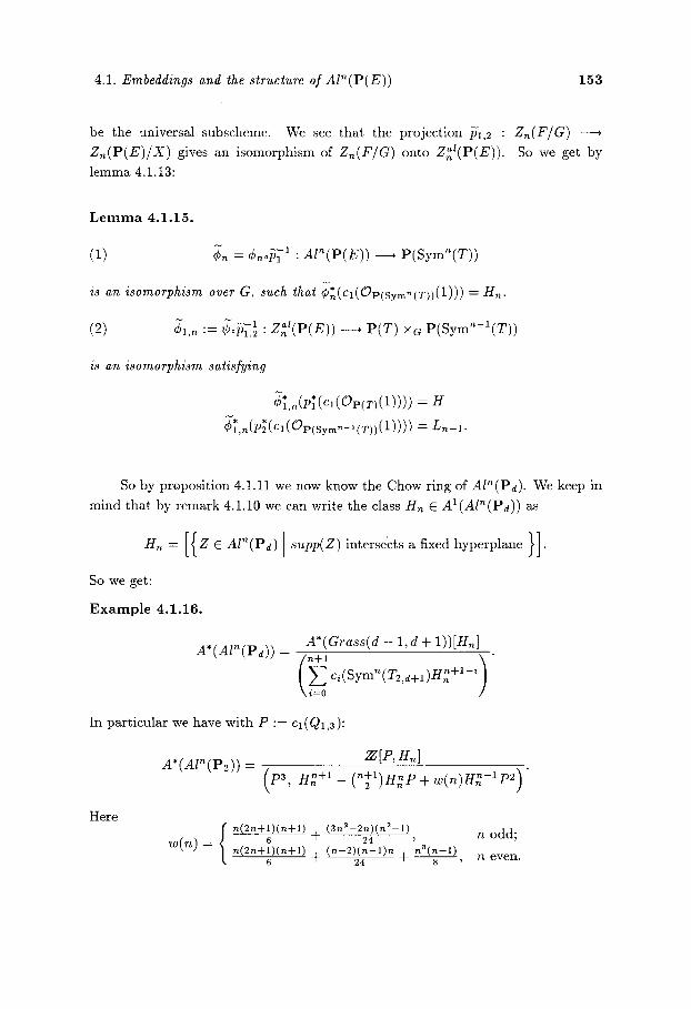
4.1. Embeddings and the structure of Aln(P( E)) 153
be the universal subscheme. We see that the projection pl,2 : Zn(F/G) ) Zn(P(E)/X) gives an isomorphism of Z~(F/G) onto Z~l (P(E) ) . So we get by
lemma 4.1.13:
L e m m a 4 . 1 . 1 5 .
(1) Cn = CnoPl 1 : AU(P(E)) ----+ P(Sym~(T) )
is an isomorphism over G, such that r = Hn.
(2) r := r : Z~ t (P(E) ) ---+ P ( T ) x a P ( S y m n - l ( T ) )
is an isomorphism satisfying
r = H
"r = Ln-1.
So by proposit ion 4.1.11 we now know the Chow ring of Aln(Pd). We keep in
mind that by remark 4.1.10 we can write the class H~ E AI(AI~(Pd)) as
H ~ = [ { Z c Aln(Pd) supp(Z)intersects a fixed hyperplane }] .
So we get:
E x a m p l e 4 .1 .16.
A*(Aln(pd)) = A*(Grass(d - - 1, d + 1))[Hn] n + l . ~ "
Z ci(Sym'~(Tz,d+l)H'~+l-') i = 0 /
In part icular we have with P := c1(Q1,3):
2~[P, H . ] A*(AIn(Pz)) = ([pa, H~+a .+1 n -( 2 ) H . P + w ( n ) H~-IP2)
Here
= { n(2n-}-l)(n-.}-l) (3n2--2n)(n2--1) 6 + 24 , n odd;
n(2n+l)(n+l) (n--2)(n--1)n n a ( n - - 1 ) 6 + 24 Jr- 8 , n e v e n .

154
~ 3 4.2. C o m p u t a t i o n of the Chow ring of Hilb (P2)
Now we want to use the results of the preceeding section to compute the Chow ~ 3
ring of the variety Hilb (P2) of triangles in P2 with a marked side. Remember that - - 3 p~2] p~3] Hilb (P2) C x is defined as the subvariety
Hil'---~a (p2) : _ -
~ 3 Hilb (P2) was defined in [Elencwajg-Le Sarz (2),(3)] to compute the Chow ring of
p~S]. The result is however quite complicated. In this section we shall see that the ~ 3
Chow ring of Hilb (P2) is relatively simple, so it might be more useful for some ~ 3
enumerative applications. If the ground field is C, then the Chow ring of Hilb (P2) ~ 3
coincides with the eohomology ring (Proposition 2.5.19). Let res : Hilb (P2) ----* P2
be the residual morphism (see lemma 2.5.3) and
~ 3 Hilb (P2)
/ P~ \ P~
p~2} p~3]
the projections. By proposition 2.5.19 we get
A~(Hil~--b3(p2)) = As(H~Ib3(P2)) = 2~ 4
A2(Hil~---b3(p2)) = A4(H~]~b3(p2))= 2g 9 ~ 3
A3(Hilb (P2)) = 2g n.
~ 3 Now we define some elements of Al(Hilb (P2)), which will generate the Chow ring
~ 3 of Hilb (P2).
Def in i t ion 4.2.1. Let Z2(P2) C P2 • p~2] be the universal subscheme and let
Z~(P2)
/p \q2
P2 p~2]
be the projections. Let H := rcs*(el(Op~(1))) and let
a x e : = A l 2 ( e : )
be the axial morphism of 4.1.14. We put
P := p~axe*(cl(Q1,3)),
H2 := p~(q2),p*(cl(Oi%(1))).
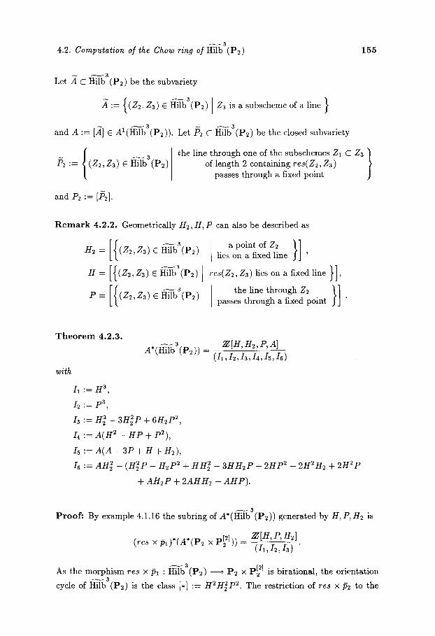
~ 3 4.2. Computation of the Chow ring of Hilb (P2) 155
N ~ 3
Let A C Hilb (Pc) be the subvariety
{ - -3 } .4 := (Z2, Za) �9 Hilb (P2) Z3 is a subscheme of a line
~ 3 ~ 3 and A := [.4] �9 Al(Hilb (P2)). Let P2 C Hilb (P2) be the closed subvariety
- - 3 the line through one of the subschemes Z1 C Z3 / /~2 := (Z2, Za) �9 Hilb (P2) of length 2 containing res(Z2, Z3)
J passes through a fixed point
and P2 := [P2I-
R e m a r k 4.2.2. Geometrically H2, H, P can also be described as
H2 = (Z2,Za) �9 Hilb (P2)
[{ - ' L n = (Z2, Z3) �9 Hilb (P2)
P = Z2, Z3) �9 Hilb (P~)
a point of Z2 }] lies on a fixed line '
res(Z2,Z3) lies on a fixed line }],
l the line through Z2 passesthroughafixedpoint }] "
T h e o r e m 4.2.3.
with
3 2g[H, H2, P, A] A*(Hilb (P2) )= ( I i , h , I 3 , I 4 , I s , I s )
/1 := H 3,
I 2 : : P 3 ,
/3 := H i - 3H22P + 6H2P 2,
/4 :-- A ( H 2 - H P + p2),
Is := A ( A - 3P + H + H2),
Is := d g ~ - ( H i P - H2P 2 + HH~ - 3 H H 2 P + 2 g P 2 - 2H2H2 + 2 H 2 P
+ A H 2 P + 2AHH2 - A H P ) .
~ 3 Proof : By example 4.1.16 the subring of A*(Hilb (P2)) generated by H, P, H2 is
2g[H, P, H2] (res • pl)*(A*(P2 x p~2])) _ (/-~,/2:/---~
3 p~2l As the morphism res x Pl : Hilb (P2) ' P2 x is birational, the orientation ~ 3
cycle of Hilb (P2) is the class [*] := H 2 H ~ P 2. The restriction of res x t52 to the

156 4. The Chow ring of relative Hilbert schemes of projective bundle~
subvariety A gives an isomorphism r .4 ----* Z~t(P2) C Z3(P2). By lemma 4.1.15 we have
al Z3 (P2) = P(T2,3 • Hilb2(p(T2,3)/152),
where T2,3 is the tautological bundle over 152 = Grass(l, 3). So we get
~ ' [H, H2, P] A*(A) = (p3,H2 _ H P + P2,H~ - 3H~P + 6H2p2) '
and the orientation cycle of A is P2HH~. So relat ion/4 = 0 holds in A (Hilb (P2)),
and for the orientation cycle we get [*] = AHH22P 2. To show Is = 0 we use the
class P2 ff AI(H~]~b3(p2)).
L e m m a 4.2.4. P + P2 = A + H + H2.
Proof : Let
H- := [ { Z E P~3] I Z intersects a fixed l ine}I,
~ : = [ { Z E p ~ 3 ] a s n b s c h e m e Z 2 o f l e n g t h 2 o f Z }] lies on a line passing through a fixed point
So we have by definition H = ( /)2) .(8) , P = (152),(P), A = / ~ ( A ) , and we see that the relations
p ~ ( n ) = H + H2,
f~ (P) = P + Pc,
(t52). (A) = 3A
3 p~3] hold, as the projection f2 : Hilb (P2) ~ is generically finite of degree 3. In
[Elencwajg-Le Barz (3)] it has been shown that the relation P = A + H holds in A 1 (p~31). We briefly repeat the elementary argument: we put
r := (P2),(HH~p2),
r := (P2),(H2H2P 2) e AS(p~3]).
These classes can be geometrically described as follows:
[ { Z consists of two distinct fixed points } ] r = Z E p~3] x l, x2 and another point x3 moving on a ,
fixed line containing neither xl nor x2 �9
,2 [/z P J Z consists of a fixed point x and ~ ] a subscheme Z2 of length 2 on a
fixed line l not containing x; Z2 contains a fixed point x2 C l.

~ 3 4.2. Computation of the Chow ring of Hilb (P2) 157
Using this description we can easily compute the intersection table:
r 1 2
r 1 1
As the group A 1(P~3]) = A5 (p~a]) is free of rank 2, we see that H, A and r r form
bases of Ax(p~ 3]) and As(P~ a]) respectively and the relation P = A + H holds. The
result follows. []
L e m m a 4 .2 .5 . A P 2 = 2AP.
P r o o f : We have to show the relation P21J~ = 2P]x. We have
~ P(T2,3) x~, 2 P(Sym2(T2,3)).
Let 71"1 : P(T2,3) ----* I52
~r2 : P(Sym2(T2,3)) -----* 152
Pl : P(T2,3) Xl~ 2 P(Sym2(T2,3)) ----* P(T2,3)
P2 : P(T2,3) xp2 P(Sym2(T2,3)) ~ P(Sym2(T2,3))
be the projections. Then we have P = p~(~r~(cl(Q1,3))). Let
.4 := P(T2,3) x~, 2 P(T2,3) xt , 2 P(T2,3),
where Pl, P2, P3 : -4 ~ P(T2,3) are the projections. We consider the natural
morphism r .4 ---+ P(T2,3) x p : P(Sym2(T2,3)). Let
:P(T2,3) xp2 P(T2,3) - - ~ 152
:P(T~,~) • P(T~,~) • P(T2,~) ----, P~
be the projections. Then we see
r =
r =
N .
r (c , (Q1,3)) ) - -
(t)2 • p3)*(~*(cx(Q~,3)))
~- (c~(Q~,3)),
* ~ ' * C (151 • ( ( 1 (Q1,3) ) )+(p l •
2~ (c1(Q1,3)),
2PIz.
The lemma follows. []

158 4. The Chow ring of relative Hilbert schemes of projective bundles
From lemmas 4.2.4 and 4.2.5 we get the relation I5 = 0:
A 2 = A ( P + P 2 - H - H 2 )
= 3 A P - A H - AH2.
The information we have obtained until now is already enough to determine the ring ~ 3
structure of A*(Hilb (P2)).
We use relations I1,. �9 �9 to compute the intersection tables. We also use that
the orientation class is [*] = A P 2 H H ~ = H2H22P 2. We get the following tables:
A 1 • A 5
H H~ P 2
H 2 H ~ p
H 2 H~ P~
AHH2 p2
3 1
1
A
1
1
- 1
A 2 • A 4
It~ P 2
H H 2 p
H H ~ P 2
H2H~
H2 H2 P
H ~ p 2
A H 2 P ~
AHH~PI
A H P ~
3 1
1
1
1
3 1
1
3 1
1
- 1
- 1 - 1
A H
1
1
- 1
- 1

~ 3 4.2. Computation of the Chow ring of Hilb (P2) 159
A 3 x A 3
H~P
H2P 2
HH~
HH2P!
H p 2
H2H2
H 2 p
AH2P
A p 2
AHH2
A H P
AH~
3 1
1
3 1
1
3 3
3 1
1
- 1
- 1 - 1
- 1
3 1
1
1 3 1
1
- 1 - 1
- 1
- 1
- 1
- 1
By solving the
We see that these conditions are only satisfied by the elements of the basis oceuring
in the above intersection matrices. []
h < 2 (i~),
p < 2 (h) ,
h2 -< 2 (h ) ,
a < 1 (h ) ,
h + a < _ 2 (14),
a + h2 <_ 2 (I6).
We see that the intersection matrices are all invertible over 2~.
system of equations given by the last intersection matrix we get 16 = 0.
~ 3 End of the p r o o f o f t h e o r e m 4.2.3: As we have found a N-basis of A*(Hilb (P2))
~ 3 consisting of monomials in H 2 , P , H , A the ring A*(Hilb (P2)) is generated by
H 2 , P , H , A . We also have seen that the relations I~ = 0 , . . . , I s = 0 hold. We
have to show that these generate all the relations. For this it is enough to show
that every monomial in H2, P, H, A can be expressed in terms of the elements of the
basis by making use of 11,. . . , Is. Let M be such a monomial. By I1 , . . . , / 6 it can
be expressed as a linear combination of monomials A~HhpPHh2 2 satisfying
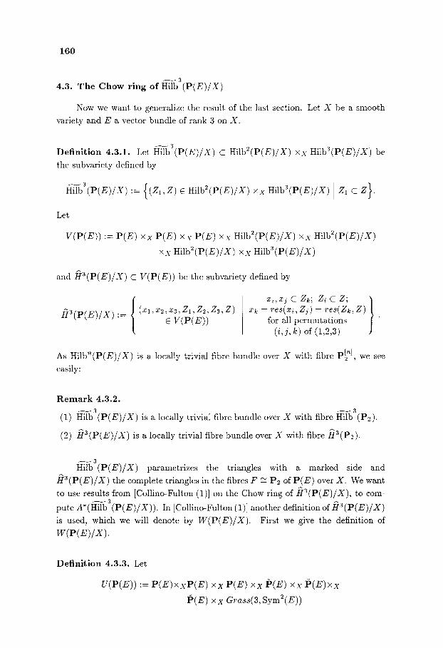
160
~ 3 4.3. T h e Chow ring of Hilb (P(E)/X)
Now we want to generalize the result of the last section. Let X be a smooth
variety and E a vector bundle of rank 3 on X.
~ 3 Defin i t ion 4.3.1. Let Hilb (P(E)/X) C Hilbe(P(E)/X) xx Hilb3(p(E)/X) be
the subvariety defined by
Hilb (P(E)/X) := (Z1,Z) E Hilb2(P(E)/X) xx Hilb3(p(E)/X) Zl C Z
Let
V ( P ( E ) ) := P ( E ) x x P ( E ) x x P ( E ) x x Hilb2(P(E)/X) xx Hilb2(p(E)/X)
xx HilbZ(P(E)/X) xx HilbZ(e(E)/X)
and s C V(P(E)) be the subvariety defined by
H3(P(E)/X) := { (xl, x2, x3, Z1, Z2, Z3, Z) C V(P(E))
xi,xj C Zk; Zi C Z; ] x~ = r ~ ( x ~ , z~) = r ~ ( z k , z )
for all permutations (i,j, k) of (1,2,3)
As Hilb~(P(E)/X) is a locally trivial fibre bundle over X with fibre P~ nl, we see
easily:
R e m a r k 4.3.2. ~ 3 ~ 3
(1) Hilb (P(E)/X) is a locally trivial fibre bundle o v e r X with fibre Hilb (P2).
(2) s is a locally trivial fibre bundle over X with fibre ~r3(P2).
N 3 Hilb (P(E)/X) parametrizes the triangles with a marked side and
Ha(P(E)/X) the complete triangles in the fibres F ~ P2 of P (E ) over X. We want
to use results from [Collino-Fulton (1)] on the Chow ring of H3(p(E)/X), to com- ~ 3
pute A*(Hilb (P(E)/X)). In [Collino-Fulton (1)] another definitionof~r3(p(E)/X) is used, which we will denote by W(P(E)/X). First we give the definition of
W(P(E)/X).
Def in i t i on 4.3.3. Let
U(P(E)) := P(E)xxP(E) • P(E) • P(E) xx P(E)•
P(E) xx Grass(3, Sym2(E))

~ 3 4.3. The Chow ring of Hilb (P (E) /X ) 161
and let s : U(P (E ) ) , X be the projection. Let x E X.
y = ( ~ , ~ , ~ , ~ , , & , ~ , r ) ~ ~-~(~)
is called a honest triangle if xa, x2, x3 are three distinct points of a fibre P (E (x ) )
and ~k is the line connecting x,, xj (for all permutations (i,j, k) of (1,2, 3)) and F
is the linear system of conics passing through xl, x2, x3, viewed as an element of
the fibre ara~43, Sym2(E(x))). Let Wo(P(E)) C U(P (E) ) be the set of honest
triangles and W ( P ( E ) ) the closure of Wo(P(E)) in U(P(E) ) .
Now we want to construct an embedding of h r a ( p ( z ) / x ) into a product of
bundles of Grassmannians. By the results of section 4.1 we get that the morphism
r x r x Cz]~3(p(E)/X ) is a closed embedding of Br3(p(E)/X) into
P(E)x x P ( E ) X x P ( E ) x x Grass(4, Sym2(E)) x x Grass(4, Sym2(E))• x
ara~s(4, Sym2(E)) x x a t (7 , Sym3(E)).
On the other hand in [Le Sarz (10)] ~r3(P2) was shown to be a closed subscheme of
p3 x p3 • Grass(3, 6), and we can see from the proof that the embedding/~3 (P2)
p~ • p3 x Grass(3, 6) is given by the morphism
(I) : : r r Op~(i),i x o~(I),2 x r
We have the morphisms
1p(E) = r : P ( E ) , P (E) ,
axe := Cop(E)(1),2 : Hilb2(P(E)/X)
r := r : Hilb3(p(E)/X)
, Grass(l, E),
Grass(3, Sym2(E)).
P r o p o s i t i o n 4.3.4.
3 := 1p(E) X axe 3 • r H3(P(E) /X) ~ U(P(E) )
is a closed embedding with image W ( P ( E ) ) .
P r o o f : Let U C X be an open subset over which E is trivial. Then with respect
to suitable local trivialisations over U the restriction of ~ is the dosed embedding
1v x ~5: U • H3(p2) , V • P~ • 15~ x Grass(3,6).
So ~ is a closed embedding. We can see immediately that the image of the open
subvariety
hrgl ' l ' l ) (P(E)) := e ~I3(p(E) /X) the xi are distinct

162 4. The Chow ring of relative Hilbert schemes of projective bundles
is the variety Wo(P(E)) C U(P(E)) of honest triangles in P(E) . As/~(31,1,1)(X ) lS
open and dense in ~r3(X) and W(P(E) ) is defined as the closure of W0(P(E)) in
U(P(E)) , the result follows. []
In [Collino-Fulton (1)1 the Chow ring of W(P(E)/X) is computed as an algebra
over A*(X). There the following classes are important:
Def in i t ion 4 .3 .5 . Let
151,f2,p3 : W(P(E) )
ql, q2, q3 : W(P(E) )
4: W(P(E) )
be the projections. We put
P ( E ) ,
, P ( E ) ,
Grass(3, Sym2(E))
a : = p;(c,(Op(E)(1))), b : = p~(r c = p~(~,(op(E)(1))),
a := ~t~(c,(T~,E)), fl : : (t~(cl(T~,E)), "7 := ~t~(cl(T~,E) )
Then a,b,c,a, fl,~f �9 AI(W(P(E))). Let 7r: P (E) ~ X, ~ : W(P(E) ) ~ X be
the projections. We write:
~ , : = ~ * ( c ~ ( E * ) ) = - ~ * ( c l ( E ) ) ,
, 2 := ~ * ( c 2 ( E * ) ) = ~ * ( c 2 ( E ) ) ,
~3 := ~ * ( c 3 ( E * ) ) = - ~ * ( c ~ ( E ) ) .
Let e �9 AI(W(P(E))) be the class of the subvaxiety
"K:= { (xl'x2'x3'(l'(2'(3'F) I � 9 W(P(E) ) F is the net of conics
on the fibre P ( E ( ~ ( x i ) ) ) ~ P~, ' con ta in ing ~1
and r �9 AI(w(P(E))) the class of
~ : = ( X l , X 2 , X 3 , ~ l , ~ 2 , ~ 3 , r ) e W(P(E) )
Xl = X2 = X3, ] F is the net of conics,
on the fibre P(E(~r(xj))) ~ P2, " having a singular point at Xl
By [Collino-Fulton (1)] we have:
L e m m a 4 .3 .6 .
(1) r = e + a + b + c + # l - ~ - f l - %

~ 3 4.3. The Chow ring o] Hilb ( P ( E ) / X ) 163
(2) (3) (4)
(5)
(6) (7)
a 3 =#la ~ - # 2 a + p a (and similarly ]orb andc),
(~3 = 2#1a2 _ (p2 + #2)~ + #1#2 -- #3 (and similarly ]or fl and 7),
a~ : a 2 + ~2 - #1~ + #2
(and similarly for a, 7; b, (~; b, 7; c, a; c, fl respectively),
Ta = Tb = TC~
6T = 0 ,
Let
Now we want to describe the classes
~*(a), ~*(b), ~*(c), ~*((~), (~*(~), ~*(7), ~*(e), ~*(r) �9 AI(Ha(P(E) /X)) .
Pl ,P2,P3 : H3(P(E) /X) ~ P(E) ,
ql, q2, q3: Ha(P(E) /X) ~ Hilb2(p(E)/X),
q: Ha(P(E) /X) ~ Hilba(P(E)/X)
be the projections.
R e m a r k 4.3.7.
~*(~) : p~(ci(O~(~)(1))), ~*(b) : p~(ci(O~(E)(1))), ~*(c) = p~(e~(O~(E)(1))),
~*(a) = q~axe*(cl(T;,E)), %*(~) = q~axe*(o(T;,E)), ~*(7) = q~axe*(c,(T;,E)).
Let A �9 AI(Hilb3(P(E)/X)) be the class of AIa(P(E)/X) . Then we have ~*(e) -- q*(A).
~*(v) is the class of the subvariety
(xl, x~, xa, Z1, Z2, Z3, Z) and with F = P(E0r (z l ))) . �9 Ha(P(E) /X) m s is the ideal of Z in OF ~
F, x l
Proof : The statements on (~*(a),~*(b), ~*(c), ~*(a), ~*(~), ~*(7) follow easily from the definitions. By definition ~*(e) is the class of the subvariety
I (xl, x2, z3, Z1, Z2, Z3, Z) 6 H3(P(E) /X)
the lines axe(Z1 ), axe(Z2), axe(Z3) ] through ZI, Z2, Z3 in the
fibre F = P(E(r(Xl))) ~ P2 are equal and r
is the net of conics in F, containing the line axe(Z1).

164 4. The Chow ring of relative Hilbert schemes of projective bundles
We consider this condit ion fibrewise. As r is the kernel of the restr ic t ion map
rz : g ~ Op2(2)) ) H~ Oz| , the condit ion on 52,3(Z), means tha t
Z is a subseheme of the line axe(Z1) through Z1. So also Z2 and Z3 are subsehemes
of axe(Z~), and the condit ions on axe(Zj) and axe(Z3) are fulfilled automatical ly .
So we get ~*(e) = q*(A).
By definition ~* ( r ) is the class of the subvariety
Xl = x2 = x3 / (xl ,xj ,x3,Z1,ZJ, Z3,Z) and r i s t h e n e t o f c o n i c s
�9 H3(p(E) /X) in the fibre P (E(z r (x l ) ) ) = PJ , " having a singular point at Xl
Let ( z l , x j , z3, ZI , Zj , Z3, Z) be a point of this subvariety. The condit ion on r
means tha t Z lies in the subscheme 5 C F = P ( E ( : r ( x l ) ) ) with suppor t xa which
is defined by m 2 in OF,~t. 2 is a subscheme of length 3 of P(E(Tr(x l ) ) ) , so we F, Xl have Z = Z. As Xl, x j , x3 are subschemes of Z, the condit ion xl = x2 = x3 follows
au tomat ica l ly fi'om the condit ion o n r The result follows, u
~ 3 Now we turn to the variety Hilb (P(E)/X) of tr iangles in the fibres of P ( E )
~ 3 ~ 3 with a marked side. Via res: Hilb (P(E)/X) , P ( E ) we regard Hilb (P(E)/X) as a subscheme of P ( E ) Xx Hilb2(p(E)/X) xx Hilb3(p(E)/X):
Hilb (P(E)/X) = x ,Z , ,Z ) x c Z1 C Z, r e s ( Z 1 , Z ) = x .
So we have a na tu ra l morphism
7n4z :-~3(P(E)/X) --~ ~lb3(P(E)/X);
( X l , X j , x 3 , Z 1 , Z J , Z 3 , Z ) , ) ( x l , Z 1 , Z )
Let
Let
~ 3 := 7r147o~ -a : W ( P ( E ) ) ----* Hilb (P(E)/X).
~ 3 p a : Hilb (P(E)/X)
~ 3 P2: Hilb (P(E)/X)
~ 3 ~ : Hilb (P(E)/X)
be the projections. Let r HilbJ(P(E)/X)
, P ( E ) ,
) Hilbz(P(E)/X),
, Hilba(p(E)/X)
, P (SymJ(T j ,E) ) be the i somorphism
from lemma 4.1.15 with ~* ~ 2 ( O P ( S y m J ( T j , E ) ) ( 1 ) ) ---- (qj) .p*(Op(E)(1)) . H e r e
Zj(P(E) /X)
~/P "~q2
P ( E ) Hilb 2 ( P ( E ) / X )

~ 3 4.3. The Chow ring of Hilb (P(E)/X) 165
are the natural projections of the universal subscheme.
Def in i t i on 4.3.8. We put
H := p~(c,(Op(E)(1))), ~* *c 1 "* ~* H2 :=p2(q2) .p I ( O p ( E ) ( ) ) =P2r
P := p"~axe*(cx(T~,E)),
A = ~'*(A).
~ 3 We want to show that H, H2, P, A generate A*(Hilb (P(E)/X)) as an A*(X)-
algebra and to determine the relations. For this we first determine the classes
~*(H), ~*(H2), ~*(P), ~*(A)E AI(W(P(E))).
L e m m a 4.3.9. ~ * ( H ) = a , ~*(H2)=b+c, ~ * ( P ) = a, ~-*(A) = e.
P r o o f : ~*(H) = a, ~*(P) = a, ~*(A) = e follow immediately from the definitions
and remark 4.3.7. Now we show ~*(H2) = b+ c. Let F(E) C P ( E ) • lb(E) be the
incidence variety
F(E) : = {(x,/) ~ P(E) • C l}
and F(E)
~/p, \p2
P ( E ) P ( E )
the projections. It is easy to see that there is an isomorphism ~ : F(E) -----+ P(T2,E) over P ( E ) with ~*(Op(T2.E)(1)) = p~(Op(E)(1)). Let
r2,a : W ( P ( E ) ) ~ ( P ( E ) x x ~ ' (E)) x x ( P ( E ) x x t)(E));
(Xl, X2, X3, El, ~2, ~3, r ) e------+ ((X2, ~2), (X3, (3)).
We see from the definitions that the image r2,3(W(P(E))) lies in the subvariety
F(E) xx F(E) of ( P ( E ) x x 15(E)) • ( P ( E ) Xx 15(E)). The diagram
W ( P ( E ) ) .... , F(E) xx F(E) *• , P(T2,E) x x P(T2,E)
Hilb (P(E)/X) ,2 - - ~ Hilb2(P(E)/X) ~ P(Sym2(T2,E))

166 4. The Chow ring of relative Hilbert 3chemes of projective bundles
commutes. Here r] is the morphism defined by the natural map T2,E | T2,E Sym2(T2,E). With respect to the projections
r l , r2 : P(T2,E) • P(T2,E) ~ P(T2,E)
we have:
rl*(Cl(OP(Sym2(T2,E))(1))) = r;(Ca(Op(T2,E)(1))) + r;(Cl(Op(T2.E)(1))).
By r = p~(Op(E)(1)) the result follows []
~ 3 Now we can give a first description of the Chow ring A*(Hilb (P(E)/X)).
~ 3 P r o p o s i t i o n 4.3.10. ~-* : A*(Hilb (P(E)/X)) , A*(W(P(E))) is injective.
~ 3 ~*(A*(Hilb (P(E)/X))) i~ the A*(X)-subalgebra of A*(W(P(E))) generated by
F*(H) = a, ~*(H2) = b + c, ~*(P) = a, ~*(A) = e.
Proof." The classes which we called A, H, H2, P in section 4.2 will now be called Ap2 , ~ 3
Hp:, H2,P2, PP2" We see that the restrictions of A, H, H2, P to a fibre Hilb (Pc) are
Ap2, Hp~, H2,p2, PP2' Then by the theorem of Leray-Hirsch for the Chow groups
[Collino-Fulton (1)] the monomials in A, H, P, H2 occuring in the intersection tables ~ 3
at the end of section 4.2 form a basis of A*(Hilb (P(E)/X)) as a free A*(X)- ~ 3
module (as Hilb (P2) has a cell decomposition). So we only have to see that ~*
is injective. Let 7rp 2 : /~3(p2) ~ 3 A , Hilb (P2) be the restriction of ~ to a fibre
03 (P2). The orientation classes [,] of Hil'-'-b 3 (P z) and [**] of HS(P2 ) fulfill ~b~ ([*]) = ~ 3
3[**], ~',([**]) = [*], as ~P2 is generically finite of degree 3. As both Hilb (P2)
and Ha(P2) have a eell decomposition, the intersection product in complementary
dimensions gives a nondegenerate pairing of free 2g-modules for both varieties. So
~* is injective. As a homomorphism of free A*(X)-modules P ~
~ 3 --~rp, | 1A*(X) : A*(Hilb (P(E)/X))
~ 3 = A*(Hilb (P2)) | A*(X) , A*(Hs(P2)) | A*(X) = A*(Hs(P(E)/X))
is one to one. So ~* is injective. []
~ 3 We now describe A*(Hilb (P(E)/X))) directly by generators and relations.
T h e o r e m 4.3 .11.
3 A*(X)[H2, P, H, A] A*(Hilb (P(E)/X)) = (I1,12, I3,14, I5,/6)

~ 3 4.3. The Chow ring of Hilb ( P ( E ) / X ) 167
w h e r t ~
/1 : = H 3 - # 1 H 2 + p e H - # a ,
/2 := P ( P - #l ) 2 + #2(P - #1) + #3,
I3 := H i - 3VH~ + H~(GV ~ - 4Pro + 4 ~ ) - 4 ( P 3 - P ~ m + P ~ ) ,
14 : = A(H 2 - P H + P ( P - #1) 21- ~2),
15 := A ( A - 3P + H + H2 + # 1 ) ,
16 := - A H ~ + # I ( - H ~ + H2P + 2HH2 - 2HP) + H2p - H2P 2 + HH~
- 3HH2P + 2HP 2 -- H2H2 + 2H2p + A(H2P + 2HH2 - 2HP).
P r o o f : We have ~'~(A*(P(E))) = A*(X)[H]/(I1). Fur thermore
P = ~axe*(ca(Ql,E)) + #1
and thus
A*(X)[P] ~axe*(A*(P(E) ) ) = ( ( p _ #1)3 + # I ( P - - #1) 2 "[- #2(P - - #1) -~- /23)
= A * ( X ) [ P I / ( h ) .
We have ~2axe*cl ( T2,E ) = - P,
~axe*c2(T2,s) = P ( P - #1) + #2.
So we get by 3.1.9
~axe*c(Sym2(T2,E)) = 1 - 3P + (6P ~ - 4P#1 + 4#2) - 4 (P 3 - P2#1 + P#2)
and thus
R e m a r k 4 .3 .12. The A*(X)-subalgebra of A * ( P ( E ) / X ) ) generated by H, P, H2
is A*(X)[H, H2, P]
(P'I • ~2)*(A*(P(E) • Hilb2(P(E)/X))) = (I1, /2, I3)
Via
~ 3 Let A C Hilb ( P ( E ) / X ) be the subvariety defined by
(x, Z1, Z) . 4 : ~ ~ 3
�9 Hilb ( P ( E ) / X )
Z lies on a line ) in the fibre P ( E ( r ( x ) ) ) / "
passing through x
~ ~ = ax~~ : .~ - - ~ ~ ' (E)

168 4. The Chow ring of relative Hilbert schemes of projective bundles
,4 is a variety over 15(E).
~ 3 ~ • ~ : Hilb ( P ( E ) / X ) ~ P ( E ) x x H i l b 3 ( p ( E ) / X )
maps fit isomorphical ly onto Z ~ t ( P ( E ) / X ) . By lemma 4.1.15 there is an isomor-
phism
"r : Z ~ t ( P ( E ) / X ) ----* P(T2,E) • P(Sym2(T2,E))
over I~(E) satisfying
(51 • wl~') (P (CI(OP(%,E)(1))) = HI X,
(Pl X 7i'1~" ) (~ (CI(OP(Sym2(T2,E))(1)) ) : H21~".
So we get A*(A) = A * ( X ) [ H , P , H2]
(I2, Iz, H 2 - P H + P ( P - #1 ) - /22) .
~ 3 The r e l a t i on /4 = 0 in A*(Hilb ( P ( E ) / X ) ) follows by [A]-- A.
In order to prove the relat ions I5 = 0, /6 = 0, we want to compute in
A * ( W ( P ( E ) ) ) and use the reations of Collino and Fulton from lemma 4.3.6. The
proof of 15 = 0 is simple.
~ * ( A ( A - 3P + H + H2 +/21)) = e(e - 3a + a + b+ c+/21)
= E ( e - o ~ - f - 7 + a + b+ c + /21)
z s
z O .
So Ix = 0 holds. In order to proof I6 = 0, we write the relat ions in such a way that
they can be appl ied formally (by subst i tut ing) .
R e m a r k 4 .3 .13 . In A * ( W ( P ( E ) ) ) the following relat ions hold:
(1) a 3 = a2/21 - a/22 +/23 and similarly for b and c,
( 2 ) a 3 =
( 3 ) ~ =
(4) 3 2 = - a 2 + a/3 + # 1 3 - - / A 2 ,
(5) 72 = - a 2 + a'~ +/217 - #2,
(6) ac = - b 2 + ba + c 2,
(7) / 3 c = - - a 2 + a/3 + c 2,
(8) 7b = - a 2 + a7 + b 2,
2#1 a2 -- (#12 + #2)a +/21/22 - - /23 and similarly for 3 and 7,
- b 2 + ba +/21a - /22 ,

N 3 4.3. The Chow ring o f Hilb ( P ( E ) / X ) 169
(9)
(10) eb =- ea + (a - b)(c + #1 - - O l - - ~),
, c = ~ , + ( , - c ) ( b + ~,1 - ~ - "y ) .
Now we jus t a p p l y these re la t ions formal ly . We get
0 = ~ * ( A ( H 2 - H P + P ( P - #1) + #2))
= ~(a ~ - - a,~ + ,~(,~ - # 1 ) + # 2 )
= --a2c -- a2#1 + a20! -t- a2/3 + ac 2 + a#2 -- aa/~
+ bec + b2#1 - bea - b2/3 - bc 2 - b#2 -t- ba~.
F u r t h e r m o r e we get
~*(n~P) = (b + ~)~ = - b 2 c - 3b2#1 -4- 4b2a + 3bc 2 + 3b#2 + c2#1 - c#2 - 2#3,
~*( n 2 P ~) = a2(b + c)
= - b 2 c - 3b2#1 -t- 2b2a + bc 2 + 2 b a # l + b#2 + c2#1 - c#2 - 2#3,
~*(HH22) = a(b 2 + 2bc + c2),
~ * ( H H 2 P ) = aa (b + c)
= a ( - b 2 + 2ba -4- c~),
~ * ( H p 2) = a a 2
= a ( - b ~ + ba + # l a - #2), ~ * ( H 2 H 2 ) = a2(b + c),
~ * ( H 2 p ) = a2a ,
" ~ * ( A H P ) = aae ,
~ * ( A H H 2 ) = a(ab + ac + 2 a p l - 2aa - a/3 - a7 + 2ae
- b 2 - 2bc - b#l + 2ba + b/3 + c 2 - c # 1 + c7),
~ * ( A H 2 P ) = ea(b + c)
= a 2 b - a2c + a2/3 - a27 + 2ac 2 + 2a#2 - 2aa/~
+ 2aae - b2/~ - 2bc 2 - b#2 4- 2ba/3 + c27 - c#2,
~ * ( A H ~ ) = e(b + c) 2
= a 2 b + a2c + 6a2#1 - 4a2a - 3 a 2 ~ - 3a27 + 4 a 2 e - 2abc
+ 2ab~ + 2ac 7 - 2a#2 - 262c - 4b2#1 + 4b2a + b2~
+ 2bc 2 - 2bc#l + 3b#2 + c27 - c#2,

170 4. The Chow ring of relative Hilbert schemes of projective bundles
^* 2 7r (H2Pl) = #l(b 2 +2bc+c2) ,
~ * ( H 2 P # I ) ---- ~ l ( - b 2 + 2b(~ + c2),
~*(HH2#I) = a#l(b + c),
"~*(HP#I) = aplc~.
Thus we have
~ * ( - A H 2 + ~ I ( - H 2 -4- H2P + 2HH2 - 2 H P ) + H 2 P - H2P 2 + HH~
- 3 H H 2 P + 2 H P 2 - H2H2 + 2 H 2 p + A ( H 2 P + 2HH2 - 2 H P ) )
---- 2(--a2c-- a2 pl + a2 0~ + a2 /3 + ac 2 + a#2 -- ao~t3
+ b2c + b2#1 - b2c~ - b2/3 - bc 2 - b#2 + bo~/3)
= 0 .
As ~* is injective, the relat ion/6 = 0 holds in A*(H~[-lb3(p(E)/X)).
E n d o f the proof of t h e o r e m 4.3.11
The monomials in A, H, H2, P occuring in the intersection tables at the end of ~ 3
4.2 form a basis of Hilb ( P ( E ) / X ) ) as a free A*(X)-module. On the other hand
using the relations I1,. �9 16 we can express any monomial M in A, H, P, H2 as an
A*(X)-linear combination of monomials of the form AaHhPVHh22 with
h ~ 2 , p < 2 , h 2 < 2 , a < l , h + a ~ 2 , a + h 2 < 2 ,
i.e. as a linear combination of these monomials. The result follows. []
In the rest of this section we look at an important special case of ~ 3 Hilb ( P ( E ) / X ) ) . We put G := Grass(d - 2, d + 1) and let T := T3,d+l be the
tautological bundle over G.
De f in i t i on 4 .3 .14. Let ~Cop3(pd) C Hilb3(pd)-- • G be the subvariety
( __3 ) Cop ( P a ) : = ( ( Z a , Z ) , E ) E H i l b (Pa) x G Z c E
Let F C P a x G be the incidence variety F := { (x ,E) e Pd • G I x C E} with
ptojections F
Pa G.

~ 3 4.3. The Chow ring of Hilb (P(E)/X) 171
There is an isomorphism r : F , P(T) over G with r = ~ 3
p~(Or, d(1)). We see immediately from the definitions that Cop (Pd) is the sub- ~ 3 ~ 3
variety Hilb (F/G) C Hilb (Pd) x G. So we get an isomorphism
~ 3 ~ 3 r Cop (Pd) ----* Hilb (P(T)/G).
The projection/51 : Coop3(Pd) - - 3 ----* Hilb (Pd) is a birational morphism (a general
subscheme of length 3 lies on exactly one plane). It is an isomorphism outside
{ - -3 } -40:= (Z1,Z) EHilb (Pd) Z lies on a line .
Over a point (Z1, Z) E A0, lying on a line l its fibre is
/ 5 1 1 ( Z 1 , Z ) = {E E a E ~) l} ~- Pd-2
The exceptional locus of 151 is
~i ~ ' P ( T 2 , T ) X15(T ) P ( S y m 2 ( T 2 , T ) ) ,
in particular it is an irreducible divisor. So we get:
~ 3 N 3 R e m a r k 4.3.15. Cop (Pc) is obtained by blowing up Hilb (Pd) along Z~t(Pd).
~ 3 Defini t ion 4.3.16. Let A',H',H2,P' ' ,#1, #2, # 3 t , t E A*(Cop (Pal)) be the classes
[{( }] A' := E, (Z1, Z)) �9 Cop (Pd) Z lies on a line ,
H' := [{(E,(Za,Z))c Coop3(pd) res(Z1,Z)lies on a fixed hyperplane }],
[{ }] H; := (E, (Z1, Z)) e Cop (Pd) supp(Z1) intersects a fixed hyperplane ,
[{(E,(Z1,Z))~3 the line passing through Za intersects a fixed }] E Cop (Pa) 2-codimensional linear subspace '
pt :z
'E{, #a := E, (Z1, Z)) E Cop (Pa)
A:=[{(E,(Z~,Z))eUoop~(Pd) linear subspace
E has a one-dimensional intersection } ] with a fixed 2-codimensional
linear subspace
#~:= [{(E,(Z1,Z))E~op3(pa) E l i e s o n a f i x e d h y p e r p l a n e }].
Then we see easily from the definitions :

172 4. The Chow ring of relative Hilbert schemes of projective bundles
R e m a r k 4.3.17.
r = A', r = H', r = H;, r = P',
g*( .1) = .'1, ;* ( .2 ) -- . ; , g*( .3) = . ;
~ 3 So theorem 4.3.12 describes the Chow ring of Cop (Pd) in terms of classes deter-
mined by the position of subschemes relative to lines and planes in Pd.

173
4.4. The Chow ring of Hilba(P(E)/X)
As in section 4.3 let E be a vector bundle of rank 3 over a smooth variety X. We ~ 3
want to use the results of the previous section about A*(Hilb ( P ( E ) / X ) ) , to com- ~ 3
pute the Chow ring A*(Hilba(p(E)/X)) of the relative Hilbert scheme. Hilb (P2) has been defined in [Elencwajg-Le Barz (3)] in order to determine the Chow ring of p~a] by generators and relations. There the following classes are introduced:
3 - - ~ p~3] Defini t ion 4.4.1. Let ~ : Hilb (P2) be the projection. Let
H, ~ ~ a 1 (e~l),
~,p,~ e A:(P~1),
5,/~ E A3(P~ 3])
be the classes defined by
,i
&
:= ~,(H), := [ { Z C P ~ a] Z l i e s o n a l i n e } ] ,
:= ~.(H~), := ~_. (p2),
:= [{ZE p~a] Z lies on a line passing through a fixed point }],
:= [{ZEP~3] Z lies on a fixed line }] ,
:= ~.(HP2).
~ 3 Here H, P E Al(Hilb (P2)) are the classes from definition 4.2.1.
[Elencwajg-Le Barz (3)1 get for instance:
T h e o r e m 4.4.2. [Elencwajg-Le Barz (3)]
(1) .fit, ft, h ,~ ,5 ,~ ,~ generate A*(P~ 3]) as a ring.
(2) Bases of the free 2~-rnodule~ A/(P~ 3]) are
i = O: 1;
i = 1 : H , i ;
i = 4: H25, tI&,tI2[z,[z2,[zD;

174 4. The Chow ring of relative Hilbert schemes of projective bundles
i = 5 :
i = 6: Iz 3.
Elencwajg and Le Barz determine all the relations between the generators. We
will first define some classes in A*(Hilb3(P(E)/X)) as relative versions of the classes
in [Elencwajg-Le Barz (3)].
~ 3 Def in i t i on 4.4.3. Let ~ : Hilb (P (E) /X ) ~ Hilb3(p(E)/X) be the projection.
Let := ~ . (H) 6 AI(Hilba(P(E)/X)),
:= ~.(H2), /5 := ~ . (p2) C A2(Hilb3(p(E)/X)),
:= ~ . (HP 2) 6 A3(Hilb3(P(E)/X)).
~ 3 Here H , P E Al(Hilb (P (E) /X) are the classes from definition 4.3.8. Let i :
AI3(P(E) /X) ~ Hilba(P(E)/X) be the embedding and
axe: AI3(p(E) /X) ----* P(E)
the axial morphism from 4.1.14. Let again T2,E be the tautological subbundle on
lb(E) and /~ := axe*(Cl(T~*E) ). We put
i := [AIa(P(E)/X)] = i,(1) 6 AI(Hilb3(P(E)/X)),
:= i.(/~) 6 A2(Hilb3(P(E)/X)),
(~ := i,(/32) 6 Aa(Hilb(P(E)/X)).
Proposition 4.4.4.
(1) H, A, h,p, ?t, (~, ~ generate A*(Hilb3(P(E)/X))) as an A*(X)-algebra.
(2) The Ai(Hilb3(P(E)/Z))) are free A*(X)-modules with basis
= O: 1;
= 1: H, fi~;
= 2: [-I2,/IA, a,[z,p;
= 3: [t3,hH,[-I2A, H?z,~,~;
= 4: [I2~,[-I~,[-I2h,[z2,hp;
= 5: [-Ih 2, [-Ihp,
- - 6 : ~3.

4.4. The Chow ring ofHilb3(p(E)/X) 175
P r o o f i (1) follows from (2). Immediate ly from the definitions we get for the fibre
F ~ p~a] of Hilb3(p(E)/X) over a point x E X:
H i t = ~ , Ai r = i i,
h i t = h, PIF = P, alF = ~,
a i r = a, ~1~ = ~.
As p~31 has a cell decomposition, we get (2) from the theorem of Leray-Hirsch for
Chow groups [Collino-Fulton (1)] and 4.4.2. []
In order to be able to compute the image of these classes under ~*, we prove
a result on the relations between ~*, ~. , ~*, ~.. Remember tha t ~ is defined by
~ : ~Ia(P(E)/X)
(zl, x2, x3, Zl, Z2, Z3, Z),
- ~ 3 Hilb (P(E)/X);
(321, Z l , Z ) .
We also consider
~2 : ~I3(p(E)/X)
(xl, x2, x3, Z1, Z2, Z3, Z)
~ 3 Hilb (P(E)/X);
(z2, Z~, Z )
Let ~ 3
Pl,2: Hilb (P(E)/X)
(x , Z l , Z ) l
, P ( E ) Xx Hilb2(P(E)/X);
, (x, Zl) .
Lemma 4.4.5. For W E ~,2(A*(P(E) x x Hilb2(P(E) /X) ) ) we have
~*~,(w) = w + ~ . ( ~ ( w ) ) .
P r o o f : Let W = ~ i ai[X/] be the representat ion of W as a linear combinat ion of N,N X classes of irreducible varieties. Then we have ~ '*~.(W) }--~i aiTr ~r.([ i]). So it is
enough to show the result for W = ~,2([Y]), where Y C P ( E ) x x Hilb2(p(E)/X) is an irreducible subvariety. By the definitions we get
[{ Hilb3(p(E)/X ) there is a subscheme Z1 C Z }] ~.p'~l,2([Y]) = Z e of length 2 with (res(Z1,Z),Z1) e Y "

176 4. The Chow ring of relative Hilbert schemes of projective bundles
So we also have
~*<~,2 ( [Y] )
E Hilb ( P ( E ) / X )
there is a subscheme ZI C Z }] of lengm 2 wah (r~(Z~, Z), Zl) C Y
[{ _ 3 }] ~-- (x, Z1 ,Z) E H i l b ( P ( E ) / X ) (TcN(Z1,Z),Z1) ~ r
+ { (x, Zl,Z)
~ 3 E Hilb ( P ( E ) / X )
there is a subscheme ZI C Z ] 1 of length 2 with x C ZI J and ( res (Z l , Z), ZI) E Y
= - , ~ , ( ~ 2 ( [ y ] ) ) . [] ; , , : ( [ Y ] ) + ^ ^ .
~ 3 So we can obtain A * ( H i l b 3 ( p ( E ) / X ) ) as a subring of A*(Hilb ( P ( E ) / X ) ) .
T h e o r e m 4.4.6. ~* : A * ( H i l b 3 ( p ( E ) / X ) ) , A*(Hil~b3(p(E)/X)) is injective,
and "~*(A*(Hilba(P(E)/X))) is the A*(X)-subalgebra generated by
~*([-I) = H + g2,
~*(A) = A,
F*([z) = H 2 + H2P - 2P 2 + 2P#1 - 2#2,
~ . (p) = p2 _ H P + HH2 _ H 2 + A H + # I ( - P + H2 + 2H + A) + pS - 2p2,
~*(a) = AP,
"~*((~) = d p 2,
"~*(~) = g ( 3 P 2 - 2H2P + H~ + H P - HH2) + A ( P 2 - H P + HH2)
+ # 1 ( 2 P 2 - 2 H 2 P + H ~ - H P + H H 2 + H 2 - A P + A H 2 - A H )
+ # 2 ( - 2 P + H2 - H) + #2( -H2 + g + A) + 2#1#2 + #3.
Proof." By proposit ion 4.4.4 A * ( H i l b 3 ( P ( E ) / X ) ) is as an A*(X)-a lgebra generated
by H , A , h , f i ,&,6,~. For each fibre F -~ P2 the map
~ 3 ~P2 := ~*]FE31 : A*(P~ 3]) - - ~ A*(Hilb (P2))
is one to one. As a homomorphism of A*(X)-modules ~* is just
~P2 | 1A*(X) : A * ( H i l b 3 ( p ( E ) / X ) ~ 3
= A*(P~ 3]) | A*(X) ---* A*(Hilb (P2)) | A * ( X ) = A * ( P ( E ) / X ) ;
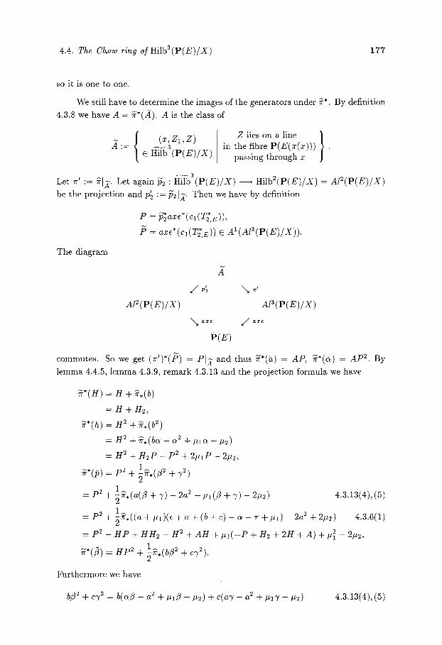
4.4. The Ckow ring of H i l b 3 ( p ( E ) / X ) 177
so it is one to one.
We still have to determine the images of the generators under ~*. By definition
4.3.8 we have A = ~*(A). A is the class of
(32, Z1, Z)
C Hilb ( P ( E ) / X )
Z lies on a line ] in the fibre P(E(Tr(z))) / '
passing through x
~ 3 Let 7r' := ~1~. Let again i~2 : Hilb ( P ( E ) / X ) , H i l b 2 ( P ( E ) / X ) = A I 2 ( p ( E ) / X )
be the projection and p~ := ~21X. Then we have by definition
The diagram
P -- ~ a x e * ( c l ( 2 , E ) ) ,
? = axe*(Cl(T~,E) ) E A ~ ( A I 3 ( p ( E ) / X ) ) .
A I 2 ( p ( E ) / X )
NNa axe
~'(E)
'"N t
A I 3 ( p ( E ) / X )
~ / axe
commutes. So we get ( # ) . ( / 5 ) = PIX and thus ~-*(~) = AP, "~*(~) = A P 2. By
l emma 4.4.5, l emma 4.3.9, remark 4.3.13 and the projection formula we have
,~*(/~) =
~*(~) =
~*(~) =
= p 2 ~_
= p 2 +
p2 _
~*(f?) =
H + ~.(b)
H + H2,
H 2 + ~.(b 2)
H 2 + ~,(bo~ - ~2 + # 1 ~ -- # 2 )
H 2 + H2P -- p2 + 2#1P - 2#2,
+ ~ . . ( 3 ~ + ~2) p2
~ ' . ( a ( / ~ -4- 3') -- -t- #1(• -I- 3') -- 2#2) 4.3.13(4), (5) 2a 2
1^ ~ r . ( ( a + # l ) ( e + a + ( b + c ) - a - ' r + # l ) - a a 2 + 2 # 2 ) 4.3.6(1)
H P + HH2 - H 2 + A H + # I ( - P + H2 + 2H + A) + #~ - 2p2,
+ 1~',(b/32 + c72). H p 2 Z
Fur thermore we have
bfl 2 "4- c72 = b(afl - a 2 -4- # l ~ - - P2) "~ c(a7 -- a 2 -f- #17 -- #2) 4.3.13(4), (5)

178 4. The Chow ring of relative Hilbert schemes of projective bundles
= - ( a 2 + ~: ) (b + c) + (a + ~ l ) (bZ + c7) ,
b9 + c7 = (b + e ) (9 + 3') - b3' - r = (b -4- c)(~ + 3') + 2a2 - a(/3 + 3') - b 2 - c 2 4.3.13(7), (8)
= 2a 2 + (b + c - a)(/~ + 7) + 2~ - (b + c)c~ - 2#1o~ + 2#2 4.3.13(3)
= 2a 2 + 2 a 2 - (b + c)(~ - 2#1a + 2#2 + e(b + c) - ea 4.3.6(1)
+ (b + c) 2 - a 2 - (b + c)(~ + ac~ - (b + c)7 + aT + (b + C)pl - a # l .
So we get
b/~ 2 + c3' 2
= a 3 + 2ae a + ae a - 2(b + c)aa - a2(b + c) + (b + c)e a - ea 2 + ea(b + c)
+ T(a(b + c) + a 2) + #l(--ac~ + (b + c)a - 2(b + c)c~ + (b + c) 2 + 2c~ 2
+ e(b + c) - ea + T(--(b ~- c) -f- a))
+ #~(-2c~ + (b + c) - a) - #2((b + c) + 2a) + 2#1#2.
Using the p ro j ec t i on fo rmula we get
~*(~) = 3 H P e + H 3 + H e p - 2 H H e P - He l l2 + H H 2 - A H 2 + A H H e
+ # I ( - H P + HH2 - 2 H e P + H~ + 2 P e + AHe - A H )
+ #21(-2P + He - H ) + # 2 ( - H e + 2 H ) + 2#1#2.
The fo rm u la for ~*(/~) is now o b t a i n e d by a p p l y i n g the re la t ions
H 3 = # 1 H e - # e H + # 3 ,
A H e = A ( H P - p e + P S i - re) . []
~ 3 As we have d e t e r m i n e d A*(Hi lb ( P ( E ) / X ) ) in t h e o r e m 4.3.11, and i ts s t ruc-
"ture is in fact r a t h e r s imple , this gives us a s imple desc r ip t ion of A * ( H i l b 3 ( p ( E ) / X ) ) ,
which is also very useful for c o mp u ta t i o n s . We now also wan t to descr ibe th is r ing
by gene ra to r s and re la t ions . Because the re la t ions are very compl i ca t ed , we d o n ' t
want to s t a t e t h e m all, b u t r a t h e r refer to [Ght tsehe (6)] for the list of all re la t ions .
T h e o r e m 4 .4 .7 .
A* ( H i l b 3 ( p ( E ) / X ) ) = A * ( X ) [ H , A, h, 15, ~, 6,/~] (R1, Re, R3, �9 �9 �9 R30)
for suitable classes R 1 , R e , R 3 , . . . , R 3 o in A*(X)[ /~ , f i~ ,h , /5 ,~ ,6~,~] , which are all
listed in Satz ~.~.7 of [Ghttsche (6)]. The relations in codimension at most three

4.4. The Chow ring of Hilb3(p(E)/X) 179
are
R2 := - / ~ p + / ~ 3 + AH5 _ 4Hh - H~ + 36 - 33
+ #1(5H 5 + 4.~/ t - 4]* - 6/5 - 3a) + #~(10/~ + 6A) + #5(-9/~r + 3.~)
+ 6#~ - 18#1#5 + 9#3,
R3 := - A h + / ~ - 36 + 3~#1 - 3fi-#5,
R4 := - . 4 p + 36,
R5 := - - ~ - H ~ + 30 - ~#i .
S k e t c h o f proof." The de te rmina t ion of the relat ions is a t r ivial but very extensive
computa t ion . We use theorem 4.4.6 and the relat ions I 1 , 1 2 , / 3 , / 4 , / 5 , / 6 of theorem
4.3.11, to express every element of the basis of K*(A*(Hilb3(p(E)/X))) over A*(X) from proposi t ion 4.4.4 as an A*(X)- l inear combinat ion of elements of the basis of
~ 3 A*(Hilb (P(E)/X)) over A*(X) from the proof of proposi t ion 4.3.10. For this we
use the computer . Similar ly we use proposi t ion 4.4.6 and the relat ions 11,. �9 �9 to
express the images of
2~ 2 ,
/~p, Ah, ~i/5, ~i~, /~4 A/~3,/~3, As, 2,3, f,~,/52, pa, as,
H36,/ .~2 ~2 ~22j), 6 2 , 6 3 , 32, B2~/5,
H h 3
~ 3 under ~* as an A*(X)- l inear combinat ion of the basis of A*(Hilb (P(E)/X)). Now
we only have to solve a system of l inear equations in order to get the relations. For
this we use again the computer . As a result we get relat ions R 1 , . . . , R30.
We still have to show tha t R 1 , . . . , R30 generate all relations. For this we have
to show tha t by using them we can express any monomial in H , A, h,/5,~, 6,3 as
an A*(X)- l inear combinat ion of the elements of the basis from propos i t ion 4.4.4.
To show this we use arguments similar to those in the end par t of the proof of
theorem 4.3.11. In the current case the arguments are however considerably more
complicated and make use of the precise form of R 1 , . . . , R30. We refer to the proof
of Satz 4.4.7 in [G6ttsche (6)] for the details. []
In the rest of this section we look at an impor t an t special case of ~ 3 Hilb ( P ( E ) / X ) ) . We put G := Grass(d - 2, d + 1) and let T := T3,u+I be the
tautological bundle over G.

180 4. The Chow ring of relative Hilbert ~cherne~ of projective bundle~
D e f i n i t i o n 4.4.8. Let Cop3(Pd) C Hilb3(pd) x G be defined by
Cop3(pd) := ~(Z,E)E HilbZ(Pd) x G Z C E~. [ 1
Let F C Pd x G be the incidence variety F := { (x ,E ) E Pd x G I z E E} with
the projections F
J Pl
P~
\ p 2
G.
~ 3 In the same way as after definition 4.3.17 for Cop (Pd) we see that there is a natural
isomorphism
~b: Cop3(pd) ----, Hilb3(p(T)/G)
over G. The projection ibl : Copz(Pd) ----, Hilb3(pd) is a birational morphism,
as every subschmeme Z of length 3 of Pd is a subscheme of a plane. This plane
is uniquely determined if Z does not lie on a line. In the same way as in the
proof of remark 4 .3 .15 we see that the f i b r e / ~ - I ( Z ) over a point Z C Al3(pd) is
isomorphic to Pd-2 and that the exceptional locus ~l(Al3(pd)) is AI3(P(T)/G) ~- P(Sym3(T2,r)) . Here again T2,T is the tautological bundle of rank 2 over P ( r ) . This
shows analogously to remark 4.3.15:
R e m a r k 4.4.9. Cop3(Pa) is the blow up of Hilb3(pd) along Al3(pd).
D e f i n i t i o n 4 .4 .10. L e t / t , A, h, ~, ~, 3, ~, #1, #2, #3 C A*(Cop3(pd)) be the classes
fi~:: [{(Z,E) CCop3(pd) Z l i e s o n a l i n e } ] ,
s [{(Z,E) ECopa(pd) Zintersectsafixedhyperplane}],
h := [{(Z,E) C Cop3(pd)
P:= [{(Z,E) EC~
3:= [{(Z,E) E Copa(pd)
Z intersec sa0xed 2 codimensiooal}l linear subspace
the line through one of the subschemes Z ~ C Z of length 2 intersects two different
fixed 2-codimensional linear subspaces
Z l i e s o n a l i n e i n t e r s e c t i n g a f i x e d }] 2-codimensional linear subspaee
}]
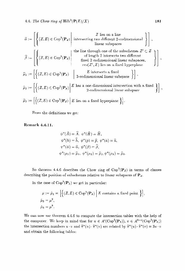
4.4. The Chow ring of Hilb3(p(E)/X) 181
F := / E) c Cop3(Pd)
: : / ' (Z,E) e Copz(Pd)
1-
Z lies on a line } ] intersecting two different 2-codimensional
linear subspaces
the line through one of the subschemes Z' C Z of length 2 intersects two different
fixed 2-codimensional linear subspaees, res(Z', Z) lies on a fixed hyperplane
E intersects a fixed }] 3-codimensional linear subspace '
}1 ~ : [ { ,~ ,~ , ~ ~op3,p~, ~ ~ ~ o ~ d ~ m e n ~ ~ 1 7 6 ~ h ~ x e d }l
2-eodimensional linear subspace
P 3 : : [{(Z,E) ECop3(pd) El i e sona f ixedhype rp l ane }].
From the definitions we get:
R e m a r k 4.4.11.
r = :~, r = ~ , r = ~, r = 3, r = ~,
r = ~, r = 5,
r = 71, r = ~2 , r = ~
So theorem 4.4.6 describes the Chow ring of Cop3(pd) in terms of classes describing the position of subschemes relative to linear subspaces of Pd.
In the case of Cop3(p3) we get in particular:
# : = / ~ 1 = [{(Z,E) ECop3(pa) E contains a fixed point }],
]52 = #2,
/~3 = 3 .
We can now use theorem 4.4.6 to compute the intersection tables with the help of the computer. We keep in mind that for u E Ai(Copa(p3)), v E A"-i(Cop3(p3)) the intersection numbers u -v and ~*(u). ~*(v) are related by ~*(u). ~*(v) = 3u-v and obtain the following tables:

1 8 2 4. The Chow ring of relative Hilbert schemes of projective bundles
A 1 x AS:
h3#2 3 2 1
:Ih~u 3 I i
A 2 x A7:
A 3 • A6:
:/2h~3 /~2a~z
h~p z
/:/&pz
h~u 3
6 3
7 6
15 6 4
3 3 1
6 -3 1
1 1 I
1 - i
2 6
3 2 4
4
1 1
- 1
3 2 1
1 1
1
~3
]~3 6 6 6 3 2 6 3 2 1
/:/h2iz 20 6 13 6 2 6 7 6 3 2 4 1 1
/ : /h)# 66 18 27 6 13 15 6 4 4 1
/~2]~#2 25 7 22 9 2 5 3 3 1 1 1
/?/2h/J2 40 9 - 1 0 - 7 - 2 2 6 - 3 1 - 1
~2~2 7 3 6 2 1 1 1
/:/ 12 2 -7 -2 1 - I
]~i~# 2 15 4 6 2 i
/:/3~3 15 3 15 6 l 3
]~/:/p 3 3 1 3 i
/~2j#3 15 3 3 -3 - I I
/Ia~ 3 6 i -3 - i
&pa 1 - 1

4.4. The Chow ring of Hilba(P(E)/X) 1 8 3
A 4 • AS:
Hh2 6 6 20 6 13 6 2 6 7 6 3 2 4 1 I
/I]~/~ 26 6 24 66 18 ! 27 6 13 15 6 4 4 1
/f/2h]~ 20 22 6 9 18 25 7 22 9 2 5 3 3 1 1 1
H2ap 22 - 1 6 6 - 8 6 40 9 - I 0 - 7 - 2 2 6 - 3 1 - 1
]~2~ 6 6 2 6 7 3 6 2 I 1 1
/~/&p 9 - 8 2 - 2 12 2 - 7 - 2 I - 1
]~i~]J 18 6 6 8 15 4 6 2 1
/:/3/~2 25 40 7 12 15 ! 15 3 15 6 1 3
]~ f/#2 7 9 3 2 4 3 1 3 1
/;/2A#2 22 -10 6 - 7 6 15 3 3 - 3 - I 1
[/~#2 9 - 7 2 - 2 6 1 - 3 - 1
&/~2 2 - 2 1
3~2 5 2 2 3
if/2# 3 3 6 i 1 1
flap 3 3 -3 1 - i
]~p3 1 1 1
d# 3 1 - I
- 1
1
j ~ 3
1

Bibl iography
Altman, A. Kleiman, S. (1) Compactifying the Picard scheme, Adv. in Math. 35 (1980), 50-112.
Andrews, G. E. (1) The Theory of Partitions, Encyclopedia of Mathematics and its Applications,
Addison-Wesley, Reading, Massachusetts 1976.
Arrondo, E., Sols, I., Speiser, R. (1) Global Moduli for Contacts, Preprint Oktober 1992.
Avritzer, D., Vainsencher, I. (1) Hilb4P2, Enumerative Geometry, Proc Sitjes 1987, S. Xamb6-Descamps, ed.,
Lecture Notes in Math. 1436, Springer-Verlag, Berlin Heidelberg 1990, 30-59.
Barth, W., Peters, C. Van de Ven, A. (1) Compact complex surfaces, Ergebnisse der Mathematik und ihrer Grenzgebiete
3. Folge, Band 4, Springer-Verlag, Berlin Heidelberg New York Tokyo 1984.
Beauville, A. (1) Vari6t6s k~ihleriennes dont la premi6re ctasse de Chern est nulle, J. Diff. Geo-
metry 18 (1983), 755-782. (2) Some remarks on K/ihler manifolds with Cl = 0, Classification of algebraic and
analytic manifolds Katata 1982, Progr. Math. 39, Birkh~iuser Boston, Boston, Mass. 1983, 1-26.
(3) Vari@t6s k~ihleriennes avee cl = 0, Geometry of K3 surfaces: moduli and peri- ods, Palaiseau 1981/1982, Ast6risque 126 (1985), 181-192.
Beltrametti, M., Sommese A. J. (1) Beltrametti, M., Sommese, A. J., Zero cycles and k-th order embeddings of
smooth projective surfaces, Cortona proceedings Problems in the Theory of Surfaces and their Classification, Symposia Mathematica XXXlI, INDAM, Aca- demic Press, London San Diego New York Boston Sydney Tokyo Toronto 1991, 33-44
Beltrametti, M., Francia, P., Sommese, A. J. (1) On Reider's method and higher order embeddings, Duke Math. Journal 58
(1989), 425-439.
Bialynicki-Birula, A. (1) Some theorems on actions of algebraic groups, Annals of Math. 98 (1973),
480-497. (2) Some properties of the decompositions of algebraic varieties determined by
actions of a torus, Bull. de l'Acad. Polonaise des Sei., S6rie des sci. math. astr. et phys. 24 (1976), 667-674.
Bialynicki-Birula, A., Sommese, A. J. (1) Quotients by C* and SL(2, C) actions, Transactions of the American Math.
Soc. 279 (1983), 45-89.

Bibliography 185
Brianqon, J. (1) Description de HilbnC{x,y}, Invent. Math. 41 (1977), 45-89.
Catanese, F., G6ttsche, L. (1) d-very-ample line bundles and embeddings of Hilbert schemes of 0-cycles,
Manuscripta Math. 68 (1990),337-341.
Cheah, J. (1) The Hodge numbers of the Hilbert scheme of points on a smooth projective
surface, preprint 1993.
Chow, W.-L., Van der Waerden, B. L. (1) Uber zugeordnete Formen und algebraische Systeme yon algebraischen Man-
nigfaltigkeiten, Math. Annalen 113 (1937), 692-704.
Colley, S. J., Kennedy, G. (1) A higher order contact formula for plane curves, Comm. Algebra 19 (1991) no.
2, 479-508. (2) Triple and quadruple contact of plane curves, Enumerative algebraic geometry
(Copenhagen 1989), Contemp. Math. 123, Amer. Math. Sot., Providence, RI, 1991, 31-59.
Collino, A. (1) Evidence for a conjecture of Ellingsrud and Str0mme on the Chow Ring of
Hilbd(p2), Illinois J. of Math. 32 (1988), 171-210.
Collino, A., Fulton, W. (1) Intersection Rings of Spaces of Triangles, Soci~t~ Math~matique de France,
Memoire 38 (1989), 75-117.
Deligne, P. (1) La conjecture de Weil, I, Inst. Hautes Etudes Sci. Publ. Math. 43 (1974),
273-307.
Digne, F. (1) Shintani descent and 1; functions on Deligne-Lustig varieties, Proceedings of
Symposia in pure Mathematics of the AMS, Volume 47 part 1, The Arcata Conference on Representations of Finite Groups 1986, 297-320.
Dixon, L., Harvey, J. Vafa, C., Witten, E. (1) Strings on orbifolds I, Nucl. Phys. B 261 (1985), 678-686. (2) Strings on orbifolds II, Nucl. Phys. B 274 (1986), 285-314.
Douady, A. (1) Le probl~me des modules pour les sous-espaces analytiques d'un est'.ace analy-
tique donn~, Ann. Inst. Fourrier (Grenoble) 16-1 (1966), 1-95.
Eisenbud, D., Harris, J. (1) Schemes: The language of moderne algebraic geometry, Wadsworth &
Brooks/Cole Advanced Books ~: Software, Pacific Grove, California 1992.

186 Bibliography
Elencwajg, G., Le Barz, P. (1) Une Base de Pic(Hilb3p2), C. R. Acad. Sci. Paris 297 (1983), 175-178. (2) D~termination de l'anneau de Chow de Hilb3P 2, C. R. Acad. Sci. Paris 301
(1985), 635-638. (3) L'anneau de Chow des triangles du plan, Comp. Math 71 (1989), 85-119. (4) Applications ~num~ratives du calcul de CH(Hilb3P2), preprint Univ. Nice
1985. (5) Explicit Computations in Hilb3P 2, Proc. Algebraic Geometry Sundance 1986,
Holme, A. and Speiser, R., eds, Lecture Notes in Math. 1311, Springer-Verlag, Berlin Heidelberg 1988, 76-100.
Ellingsrud, G. (1) Another proof of the irreducibility of the punctual Hilbert scheme of a smooth
surface, preprint 1992.
Ellingsrud, G., Strcmme, S. A. (1) On the homology of the Hilbert scheme of points in the plane, Invent. Math.
87 (1987), 343-352. (2) On a cell decomposition of the Hilbert scheme of points in the plane, Invent.
Math 91 (1988), 365-370. (3) On generators for the Chow ring of fine moduli spaces on p2, preprint 1989. (4) Towards the Chow ring of the moduli space for stable sheaves on p2 with Cl = 1,
preprint 1991. (5) Towards the Chow ring of the Hilbert scheme of P2, J. reine angew. Math.
441 (1993), 33-44.
Fantechi, B., Ghttsche, L. (1) The cohomology ring of the Hilbert scheme of 3 points on a smooth projective
variety, J. reine angew. Math. 439 (1993), 147-158.
Fogarty, J. (1) Algebraic families on an algebraic surface, American Journal of Math. 90
(1968), 511-521. (2) Algebraic families on an algebraic surface II, the Picard scheme of the punctual
Hilbert scheme, Amercan Journal of Math. 95 (1973), 660-687. Fulton, W. (1) Intersection Theory, Ergebnisse der Mathematik und ihrer Grenzgebiete,
Springer-Verlag, Berlin Heidelberg New York Tokyo 1984. (2) Introduction to intersection theory in algebraic geometry, CBMS Regional Conf.
Ser. in Math. vol. 44, AMS, Providence, R. I., 1984.
Ghttsche, L. (1) Die Betti-Zahlen des Hilbert-Schemas ffir Unterschemata der L~inge n auf einer
glatten Flgche, Diplomarbeit, Bonn, Juli 1988. (2) The Betti numbers of the Hilbert scheme of points on a smooth projective
surface, Math. Ann. 286 (1990), 193-207. (3) Identification of very ample line bundles on S [d, Appendix to: Beltrametti,

Bibliography 187
M., Sommese, A. J., Zero cycles and k-th order embeddings of smooth pro- jective surfaces, Cortona proceedings Problems in the Theory of Surfaces and their Classification, Symposia Mathematica XXXII, INDAM, Academic Press, London San Diego New York Boston Sydney Tokyo Toronto 1991, 44-48.
(4) Betti numbers for the Hilbert function strata of the punctual Hilbert scheme in two variables, Manuscripta Math. 66 (1990), 253-259.
(5) The Betti numbers of higher order Kummer varieties of surfaces, preprint 1989. (6) Hilbertschemata nulldimensionaler Unterschemata glatter Variets thesis
1991.
G6ttsche, L., Soergel W. (1) Perverse sheaves and the cohomology of Hilbert schemes of smooth algebraic
surfaces, Math. Ann. 296 (1993), 235-245.
Granger, M. (1) G6om6trie des sch6mas de Hilbert ponctuels, M6m. Soc. Math. France 8
(1983).
Griffiths, P., Harris, J. (1) Principles of Algebraic Geometry, Wiley and Sons, New York (1978).
Grothendieck, A. (1) Techniques de construction et th6or~mes d'existence en g6om6trie alg6brique
IV: Les sch6mas de Hilbert, S6minaire Bourbaki expos6 221 (1961), IHP, Paris.
Harder, G. , Narasimhan, M. S. (1) On the Cohomology Groups of Moduli Spaces of Vector Bundles on Curves,
Math. Ann. 212 (1975), 215-248.
Hartshorne, R. (1) Connectedness of the Hilbert scheme, Publ. Math. IHES 29 (1966), 261-304. (2) Algebraic Geometry, Graduate Texts in Mathematics 52, Springer-Verlag, New
York Heidelberg Berlin (1977).
Hirschowitz, A. (1) Le group de Chow ~quivariant, C. R. Acad. Sci. Paris 298 (1984).
Hirzebruch, F. (1) Topological Methods in Algebraic Geometry, Grundlehren der mathematischen
Wissenschaften 131, third Edition, Springer-Verlag, Berlin Heidelberg New York 1978.
Hirzebruch, F. with Berger, T. Jung, R. (1) Manifolds and Modular Forms, Vieweg, Braunschweig/Wiesbaden, 1992.
Hirzebruch, F., HSfer, T. (1) On the Euler number of an orbifold, Math. Ann 286 (1990), 255-260.
Iarrobino, A. (1) Reducibility of the families of 0-dimensional schemes on a variety, Invent. Math.
15 (1972), 72-77.

188 Bibliography
(2) Punctual Hilbert schemes, Bull. Amer. Math. Soc. 78 (1972), 819-823. (3) An algebraic fibre bundle over P1, that is not a vector bundle, Topology 12
(1973), 229-232. (4) Punctual Hilbert schemes, Mem. Amer. Math. Soc. 188 (1977). (5) Hilbert scheme of points: an Overview of last ten Years, Proceedings of Sym-
posia in pure Mathematics of the AMS, Volume 46 part 2, Algebraic Geometry 1985, 297-320.
Iarrobino, A., Yameogo, J. (1) Cohomology groups of the family GT of graded algebra quotients of k[[x, y]]
having Hilbert function T; and the hook differences of partitions with diagonal lengths T, preprint 1990.
(2) Partitions of diagonal lengths T and ideals in k[[x, y]], preprint 1991.
Keel, S. (1) Functorial construction of Le Barz's triangle space with applications, Trans.
Amer. Math. Soc. 335 (1993), 213-229.
Kirwan, F. C. (1) Cohomology of Quotients in Symplectic and Algebraic Geometry, Princeton
University Press, Princeton, New Jersey 1984.
Kleiman, S. L. (1) The transversality of the general translate, Compositio Math. 28 (1974), 287-
297. (2) Multiple-point formulas I: iteration, Acta Math. 147 (1981), 287-297. (3) Multiple point formulas II: the Hilbert scheme, Enumerative Geometry, Proc
Sitjes 1987, S. Xambd-Descamps, ed., Lecture Notes in Math. 1436, Springer- Verlag, Berlin Heidelberg 1990, 101-138.
(4) Rigorous foundation of Schubert's enumerative calculus, Math. Development from Hilbert problems, Proceedings of Symposia in pure Mathematics of the AMS, Volume 28 (1983), 445-482.
(5) Intersection Theory and enumerative Geometry, Proceedings of Symposia in pure Mathematics of the AMS, Volume 46 part 2, Algebraic Geometry 1985, 321-370.
Le Barz, P. (1) G~omdtrie ~numerative pour les multis~cantes, Vari~t~s Analytiques Compacts,
Proc. Conf. Nice 1977, Lecture Notes in Math. 683, Springer-Verlag, Berlin Heidelberg 1978, 116-167.
(2) Validit~ de certaines formules de gfiom~trie ~numfirative, C. R. Acad. Sci. Paris 289 (1979), 755-759.
(3) Quadrisficantes d'une surface de ph, C. R. Acad. Sci. Paris 291 (1980), 639- 642.
(4) Formules pour les multis~cantes des surfaces, C. R. Acad. Sci. Paris 292 (1981), 797-800.
(5) Formules multis6cantes pous les courbes gauches quelconques, Enumerative and

Bibliography 189
classical algebraic Geometry, Nice 1981, Prog. in Math. 24, Birkhs 1982, 165-197.
(6) Platitude et non-platitude de certaines sous-sch6mas de Hilbkp N, Journal fiir die Reine und Angewandte Mathematik 348 (1984), 116-134.
(7) Contribution des droites d'une surface s ses multis~cantes, Bull. Soc. Math. France 112 (1984), 303-324.
(8) Quelques cMculs dans les vari~t~s d'alignements, Adv. in Math. 64 (1987), 87-117.
(9) Formules pour les tris6cantes des surfaces alg~briques. Enseign. Math. 33 no 1-2 (1987), 1-66.
(10) La vari~t~ des triplets complets, Duke Math. Journal 57 (1988), 925-946. (11) Quelques formules multis~cantes pour les surfaces, Enumerative Geometry, Proc
Sitjes 1987, S. XambS-Descamps, ed., Lecture Notes in Math. 1436, Springer- Verlag, Berlin Heidelberg 1990, 151-188.
Macdonald, I. G. (1) The Poincar6 polynomial of a symmetric product, Proc. Camb. Phil. Soc. 58
(1962), 563-568.
Mallavibarrena, R., (1) Les groupes de Chow de Hilb4P 2, C. R. Acad. Sci. Paris 303, I13 (1986). (2) Validit~ de la formule classique des tris~cantes stationaires, C. R. Acad. Sci.
Paris 303, I16 (1986). (3) E1 M~todo de las bases de los grupos de Chow de Hilbdp 2 en geometria enu-
merativa, Thesis 1987.
Mallavibarrena, R., Sols, I. (1) Bases for the homology groups of the Hilbert scheme of points in the plane,
Comp. Math. 74 (1990), 169-202.
Matsumura, H. (1) Commutative Algebra, W. A. Benjamin, Inc., New York 1970.
Mazur, B. (1) Eigenvalues of Frobenius acting on algebraic varieties over finite fields, Proceed-
ings of Symposia in Pure Mathematics Vol. 29, Algebraic Geometry, Arcata 1974, 231-261.
Milne, J. S. (1) Etale Cohomology, Princeton Math. Series 33, Princeton University Press,
Princeton 1980.
Mumford D. (1) Lectures on curves on an algebraic surface, Annals of Math. Studies vol. 59,
Princeton 1966. (2) The Red Book on Varieties and Schemes, Lecture Notes in Mathematics 1358,
Springer-Verlag, Berlin Heidelberg 1988.

190 Bibliography
Mumford, D. Fogarty, J. (1) Geometric invariant theory, Ergebnisse der Mathematik und ihrer Grenzgebie-
te, second edition, Springer-Verlag, New York Heidelberg Berlin 1982.
Reider, I. (1) Vector bundles of rank 2 and linear systems on algebraic surfaces, Ann.
Math. 127 (1988), 309-316. of
Roan, S. S. (1) On the generalization of Kummer surfaces, J. Diff. Geom. 30 (1989) 523-537.
Roberts, J. (1) Old and new results about the triangle variety, Proc. Algebraic Geometry
Sundance 1986, Holme, A. and Speiser, R., eds, Lecture Notes in Math. 1311, Springer-Verlag, Berlin Heidelberg 1988, 197-219.
Roberts, J. Speiser, R. (1) Schubert's enumerative geometry of triangles from a modern viewpoint, Alge-
braic Geometry, Proc. Conf. Chicago Circle 1980, Lecture Notes in Math. 862, Springer Verlag, Berlin Heidelberg 1981, 272-281.
(2) Enumerative geometry of triangles I, Comm in Alg. 12(9-10) (1984), 1213-1255. (3) Enumerative geometry of triangles II, Comm in Alg. 14(1) (1986), 155-191. (4) Enumerative geometry of triangles III, Comm in Alg. 15(9) (1987), 1929-1966.
Rossell6 Llompart, F. (1) Les groupes de Chow de quelques sch@mas qui param@trisent des points
coplanaires, C. R. Acad. Sci. Paris S~r. I Math. 303 (1986), 363-366. (2) The Chow-Ring of Hilb3p 3, Enumerative Geometry, Proc Sitjes 1987, S.
Xamb6 Descamps, ed., Lecture Notes in Math. 1436, Springer-Verlag, Berlin Heidelberg 1990, 225-255.
Rossell6 Llompart, F., Xamb6 Descambs, S. (1) Computing Chow groups, Proc. Algebraic Geometry Sundance 1986, Holme,
A. and Speiser, R., eds, Lecture Notes in Math. 1311, Springer-Verlag, Berlin Heidelberg 1988, 220-234.
(2) Chow groups and Horel-Moore schemes, Ann. Math. Pura Appl. (4) 160 (1991), 19-40.
Schubert, H. (1) Kalkfil der abzghlenden Geometrie, Teubner, Leibzig 1879, reprinted by
Springer-Verlag, Berlin 1979. (2) Anzahlgeometrische Behandlung des Dreiecks, Math. Ann. 17 (1880), 153-212.
Speiser, R. (1) Enumerating contacts, Proceedings of Symposia in pure Mathematics of the
AMS, Volume 46 part 2, Algebraic Geometry 1985, 401-418.

Bibliography 191
Semple, J. G. (1) Some investigations in the geometry of curve and surface elements, Proc. Lon-
don Math. Soc. 4(3) (1954), 24-49. (2) The triangle as a geometric variable, Mathematica 1 (1954), 80-88.
Steenbrink, J. H. M. (1) Mixed Hodge Structures on the vanishing cohomology, Nordic Summer School,
Symposium in Mathematics, Oslo 1970, Sijthoff and Noordhoff, Alphen an den Rijn 1977, (525-563).
Tyrrell, J. A. (1) On the enumerative geometry of triangles, Mathematica 6 (1959), 158-164.
Tyurin, A. N. (1) Cycles, curves and vector bundles on an algebraic surface, Duke Math. J. 54
(1987), 1-26.
Zagier, D. (1) Equivariant Pontrjagin classes and applications to orbit spaces, Lecture Notes
in Math. 290, Springer-Verlag, Berlin Heidelberg New York 1972. (2) Note on the Landweber-Stong elliptic genus, Elliptic Curves and Modular Forms
in Algebraic Topology, Proceedings Princeton 1986, P.S. Landweber (Ed.), Lec- ture Notes in Mathematics 1326, Springer-Verlag, Berlin Heidelberg New York 1988, 216-224.

I n d e x
axial morphism 152, 154, 161, 163, 165, 167, 174, 177 Borel-Moore homology 19
cell decomposition 12, 19-28, 34, 79, t66, 175 Chern classes of symmetric powers 93, 114, 150 constant over T 148, 149 contact 81, 99
- bundle 88, 108, 115-118, 119, 121 - with lines 124-125, 128-142 - of families of curves 85, 143
- with linear subspaces 119-125
second order 122, 126 cycle map 19 degeneracy
- locus 98, 119, 123-124 - cycle 98, 119
evaluation morphism 115, 119, 122-124 formula of Macdonald 35, 49, 50, 79 geometric Frobenius 5, 7, 31, 43 good reduction 5, 6, 35, 49, 63, 78 higher-order Kummer varieties 12, 40-59 Hilbert-Chow morphism 4, 32, 40, 42, 54, 61 Hilbert function 9
- strata 9-11, 16-18, 23-28, 64, 67, 74, 91, 97, II0, 131 Hilbert polynomial I Hilbert scheme I-4
- of subschemes of length n 2
punctual - 9-11, 19, 29, 30, 33 of aligned subschemes 133, 138, 145, 151-153, 155, 156, 163, 168, 171,174,
177, 180
relative- 2, 147-149
relative - of projective bundles 145-184 - for coplanar subschemes 145, 170, 180 stratification of by partitions 3, 14, 30, 60, 67
incidence variety 133-137, 140, 152, 165, 170, 180 initial
- degree 9 form 9, 18
jet-bundle 14, 85, 90, 104, 110, 111,119 jumping index 10, 28 /-adic cohomology 5 Leray-Hirsch for Chow groups 166, 175 modular forms 35, 52

Index 193
mult ipl icat ive group 19m21 n-very ample 146
relat ive - 147-149
one-paramete r subgroup 21
general - 21, 25, 80 orbifold Euler number 12, 54-56
par t i t ion 3, 20, 22, 26, 29, 42, 44
graph of - 23
dual - 23
hook difference of 23 point
geometric -
k-valued -
T-valued -
division -
Por teous formula
4, 5, I0, 15, 29 2 1
43 98, 99, 120, 123-124
representable functor I, 60, 63, 83, 101, 102, 109 residual morphism 61, 63, 154, 155, 160, 164, 171, 176, 181 Semple-bundle varieties 128-144
relative - 142-144 Schubert cycle 135, 138, 139 Segre class 98, 124 Shintani-descent 41 symmetric power of a variety 3, 7, 32, 34, 54, 150 universal subscheme 2, 62, 65, 83, 88, Ii0, 116, 147, 149, 151,152,154, 156, 164 varieties of t r iangles 12, 60-80
complete tr iangles 63-73, 79, 85
- with a chosen side 60-62
varieties of higher order d a t a 101-127,
- of curves 85, 91, 94, 113, 114, 118 varieties of second order da t a 81-100
relat ive - 126-127
Weil conjectures 5-8, 29, 35, 41, 49, 74 zero-cycle 3, 40
pr imit ive - 8, 31-34, 45, 75
zeta-funct ion 5

Index of notat ions
~ilb(X/T) Hilb(X/T) Hilb~(X/T) X["], Hilb"(X)
Z,.(X/T), Zn(X) a(,~) X(n) X (') x~,q r n
Hi(X, qt )
p(x, z) z~(x, t) b~(x) P~(X,F~) Hilb'~(R/m"), Hilb"(R)~, t
ZT, GT (~,)~>0 A, A '~
J.(X), J~(X) zT(x), a~(x)
A.(X), A*(X) el G.. p(n), p(~, l) r(~) .&
ti(a), T(a) h~,v(~) Y. *'(~) ( n l , . . . , n ~ ) = (1~ ' ,2~2, . . . ) Gal( ]c / k )
fen(f) P(X, •q) Tn(X, Fq) A(~-), ~(~-)
Hilbert functor
relative Hilbert scheme
relative Hilbert scheme of subschemes of length n
Hilbert scheme of subschemes of length n
universal family
symmetric group on n letters
symmetric power
stratum of X (n)
stratum of X[']
Hilbert-Chow morphism
l-adic cohomology
Poincard polynomial
zeta function
Betti number
set of primitive cycles
punctual Hilbert scheme
Hilbert function strata
jumping index
(thickened) diagonal
jet bundles
relative Hilbert function strata
curvilinear subschemes concentrated in a point
Chow ring
cycle map
multiplicative group
number of partitions of n
graph of partition
dual partition
diagonal lengths of partition
hook difference
punctual Hilbert scheme
set of partitions of n
partitions
Galois group
length of subseheme
"length" of function
primitive 0-cycles
set of admissible functions
Delta function, eta function
1
2
2
2
2
3
3
3
4
4
5
5
5
5 8
10
10
10
14
14
17
18
19
19
19
20
23
23
23
23
29
29
29
29
29
30
31
31
35

Index of notation3 195
hP'q(X) h(X,x,y) sign(X) xdx) G ~ Is KAn-1 NH/H, s[.] ~l(n) e(x, G) ~ n
Hilb (X)
r e s
~3(x) _~[3] ~ 3
Hilb (Z) Grass(m, E)
";rm,E
Grass(m, r) P(E) , P ( E ) Tm,~, Tm,r Qm,E, O,,,,r Z1 �9 Z2 D~(X) T1, Qi w~(x) b~(x) I'2, Q2 (ox)~ Ar A~
Dz,=(Y) Vk(~) nn(x ) F .G W~(X) 5 ~ ( x ) , b L l ( x ) Ts, 03 (E)~n eVE
D~(Y/T) g(x , YT) Fn(X), an(x)
Hodge number
Hodge polynomial
signature
xy(X)-genus
modular forms higher order Kummer variaties
Shintani descent
set used for counting
sum of numbers dividing n orbifold Euler number
incidence variety of subschemes of lengths n - 1 and n
residual morphism
variety of complete triangles variety of complete unordered triangles
complete triangles with marked side
Grassmannian bundle projection in Grassmannian bundle
Grassmannian
projectivized bundle
tautological subbundles
universal quotient bundles
scheme defined by product of ideals
variety of second order data
tautological and quotient bundle over Grass(m, T~ ) bundle of second order data
other construction of D~(X) tautological and quotient bundle over D2(X)
contact bundle (thickened) diagonals of morphism
Ith-order datum of Y at x
degeneracy locus
variety of higher order data
"product" of sheaves
third order data sheaf
variety of third order data tautological subbundle and quotient of W3(X)
contact bundle
evaluation map relative data variety
class of second order contact
Sample bundles
37
37
37
37
38 40
42
42
51 54
60
61
63 67
71
82
82
82
82
82
82
82
83
85
86
87
87
88
88
97 98
101
105
105 107
107
108
115 126
126
128

196 Index of notations
AI~(PN) aligned n-tuples Kn(X), Kn,l(Z) class of contact with lines Fn(X/T), Gn(X/T) relative Semple bundles r163 morphism of Hilbert scheme induced by/3 Hilbn(P(E)/X) relative Hilbert scheme of projective bundle era,n, Cn morphisms of Hilbert schemes of projective bundle AI~(P(E)), Al~(Pd) variety of aligned subschemes Z~'(P(E)), Z~t(Pd) universal subscheme of aligned subschemes axe ~ axial morphism
~ 3 H, A, H2, P, P2 classes in the Chow ring of Hilb (P2) ~ 3 Hilb (P(E)/X), W(P(E)), H3(P(E)/X) relative triangle varieties ~ 3 Cop (Pd) variety of triangles in a plane in Pd H, ,zl, fz, fi, 6,/~ classes in the Chow ring of Hilb3(P(E)/X) Cop3(pd) Hilbert scheme of subschemes in a plane in Pd
135 140 144 146 149 149 151 151 152
154
160
170 173 180
Printing: Weihert-Druck GmbH, Darmstadt Binding: Buchbinderei Schiiffer, Griinstadt

Vol. 1478: M.-P. Malliavin (Ed.), Topics in Invariant Theory. Seminar 1989-1990. VI, 272 pages. 1991.
Vol. 1479: S. Bloch, I. Dolgachev, W. Fulton (Eds.), Algebraic Geometry. Proceedings, 1989. VII, 300 pages. 1991.
Vol. 1480: F. Dumortier, R. Roussarie, J. Sotomayor, H. Zoladek, Bifurcations of Planar Vector Fields: Nilpotent Singularities and Abelian Integrals. VIII, 226 pages. 1991.
Vol. 1481: D. Ferns, U. Pinkall, U. Simon, B. Wegner (Eds.), Global Differential Geometry and Global Analysis. Proceedings, 1991. VIII, 283 pages. 1991.
Vol. 1482: J. Chabrowski, The Dirichlet Problem with L z- Boundary Data for Elliptic Linear Equations. VI, 173 pages. 1991.
Vol. 1483: E. Reithmeier, Periodic Solutions of Nonlinear Dynamical Systems. VI, 171 pages. 1991.
Vol. 1484: H. Delfs, Homology of Locally Semialgebraic Spaces. IX, 136 pages. 1991.
Vol. 1485: J. Az6ma, P. A. Meyer, M. Yor (Eds.), S6minaire de Probabilit6s XXV. VIII, 440 pages. 1991.
Vol. 1486: L. Arnold, H. Crauel, J.-P. Eckmann (Eds.), Lyapunov Exponents. Proceedings, 1990. VIII, 365 pages. 1991.
Vol. 1487: E. Freitag, Singular Modular Forms and Theta Relations. VI, 172 pages. 1991.
Vol. 1488: A. Carboni, M. C. Pedicchio, G. Rosolini (Eds.), Category Theory. Proceedings, 1990. VII, 494 pages. 1991.
Vol. 1489: A. Mielke, Hamiltonian and Lagrangian Flows on Center Manifolds. X, 140 pages. 1991.
Vol. 1490: K. Metseh, Linear Spaces with Few Lines. XIII, 196 pages. 1991.
Vol. 1491: E. Lluis-Puebla, J.-L. Loday, H. Gillet, C. Soul~, V. Snaith, Higher Algebraic K-Theory: an overview. IX, 164 pages. 1992. Vol. 1492: K. R. Wicks, Fractais and Hyperspaces. VIII, 168 pages. 1991.
Vol. 1493: E. Beno~t (Ed.), Dynamic Bifurcations. Proceedings, Luminy 1990. VII, 219 pages. 1991.
Vol. 1494: M.-T. Cheng, X.-W. Zhou, D.-G. Deng (Eds.), Harmonic Analysis. Proceedings, 1988. IX, 226 pages. 1991.
Vol. 1495: J. M. Bony, G. Grnbb, L. H6rmander, H. Komatsu, J. Sj0strand, Microlocal Analysis and Applications. Montecatini Terme, 1989. Editors: L. Cattabriga, L. Rodino. VII, 349 pages. 1991.
Vol. 1496: C. Foias, B. Francis, J. W. Helton, H. Kwakernaak, J. B. Pearson, H| Theory. Como, 1990. Editors: E. Mosca, L. Pandolfi. VII, 336 pages. 1991.
Vol. 1497: G. T. Herman, A. K. Louis, F. Natterer (Eds.), Mathematical Methods in Tomography. Proceedings 1990. X, 268 pages. 1991.
Vol. 1498: R. Lang, Spectral Theory of Random SchrOdinger Operators. X, 125 pages. 1991.
Vol. 1499: K. Taira, Boundary Value Problems and Markov Processes. IX, 132 pages. 1991.
Vol. 1500: J.-P. Serre, Lie Algebras and Lie Groups. VII, 168 pages. 1992.
Vol. 1501: A. De Masi, E. Presutti, Mathematical Methods for Hydrodynamic Limits. IX, 196 pages. 1991.
Vol. 1502: C. Simpson, Asymptotic Behavior of Mono- dromy. V, 139 pages. 1991.
Vol. 1503: S. Shokranian, The Selberg-Arthur Trace Formula (Lectures by J. Arthur). VII, 97 pages. 1991.
Vol. 1504: J. Cheeger, M. Gromov, C. Okonek, P. Pansu, Geometric Topology: Recent Developments. Editors: P. de Bartolomeis, F. Tricerri. VII, 197 pages. 1991.
Vol. 1505: K. Kajitani, T. Nishitani, The Hyperbolic Cauchy Problem. VII, 168 pages. 1991.
Vol. 1506: A. Buium, Differential Algebraic Groups of Finite Dimension. XV, 145 pages. 1992.
Vol. 1507: K. Hulek, T. Peternell, M. Schneider, F.-O. Schreyer (Eds.), Complex Algebraic Varieties. Proceedings, 1990. VII, 179 pages. 1992.
Vol. 1508: M. Vuorinen (Ed.), Quasiconformal Space Mappings. A Collection of Surveys 1960-1990. IX, 148 pages. 1992.
Vol. 1509: J. Aguad6, M. Castellet, F. R. Cohen (Eds.), Algebraic Topology - Homotopy and Group Cohomology. Proceedings, 1990. X, 330 pages. 1992.
Vol. 1510: P. P. Kulish (Ed.), Quantum Groups. Proceedings, 1990. XII, 398 pages. 1992.
Vol. 1511: B. S. Yadav, D. Singh (Eds.), Functional Analysis and Operator Theory. Proceedings, 1990. VIII, 223 pages. 1992.
Vol. 1512: L. M. Adleman, M.-D. A. Huang, Primality Testing and Abelian Varieties Over Finite Fields. VII, 142 pages. 1992.
Vol. 1513: L. S. Block, W. A. Coppel, Dynamics in One Dimension. VIII, 249 pages. 1992.
Vol. 1514: U. Krengel, K. Richter, V. Warstat (Eds.), Ergodic Theory and Related Topics II1, Proceedings, 1990. VIII, 236 pages. 1992.
Vol. 1515: E. Ballico, F. Catanese, C. Ciliberto (Eds.), Classification of Irregular Varieties. Proceedings, 1990. VII, 149 pages. 1992.
Vol. 1516: R. A. Lorentz, Mult ivar ia te Birkhoff Interpolation. IX, 192 pages. 1992.
Vol. 1517: K. Keimel, W. Roth, Ordered Cones and Approximation. VI, 134 pages. 1992.
Vol. 1518: H. Stichtenoth, M. A. Tsfasman (Eds.), Coding Theory and Algebraic Geometry. Proceedings, 1991. VIII, 223 pages. 1992.
Vol. 1519: M. W. Short, The Primitive Soluble Permutation Groups of Degree less than 256. IX, 145 pages. 1992.
Vol. 1520: Yu. G. Borisovich, Yu. E. Gliklikh (Eds.), Global Analysis - Studies and Applications V. VII, 284 pages. 1992.
Vol. 1521: S. Busenberg, B. Forte, H. K. Kuiken, Mathematical Modelling of Industrial Process. B ari, 1990. Editors: V. Capasso, A. Fasano. VII, 162 pages. 1992.
Vol. 1522: J.-M. Delort, F. B. I. Transformation. VII, 101 pages. 1992.
Vol. 1523: W. Xue, Rings with Morita Duality. X, 168 pages. 1992.
Vol. 1524: M. Coste, L. Mah6, M.-F. Roy (Eds.), Real Algebraic Geometry. Proceedings, 1991. VIH, 418 pages. 1992.

Vol. 1525: C. Casacuberta, M. Castel let (Eds.), Mathematical Research Today and Tomorrow. VII, 112 pages. 1992.
Vol. 1526: J. Az6ma, P. A. Meyer, M. Yor (Eds.), S~minaire de Probabilit6s XXVI. X, 633 pages. 1992.
Vol. 1527: M. I. Freidlin, J.-F. Le Gall, Ecole d'Et6 de Probabilit6s de Saint-Flour XX - 1990. Editor: P. L. Hennequin. VIII, 244 pages. 1992.
Vol. 1528: G. Isac, Complementarity Problems. VI, 297 pages. 1992.
Vol. 1529: J. van Neerven, The Adjoint o fa Semigroup of Linear Operators. X, 195 pages. 1992.
Vol. 1530: J. G. Heywood, K. Masuda, R. Rautmann, S. A. Solonnikov (Eds.), The Navier-Stokes Equations II - Theory and Numerical Methods. IX, 322 pages. 1992.
Vol. 1531: M. Stoer, Design of Survivable Networks. IV, 206 pages. 1992.
Vol. 1532: J. F. Colombeau, Multiplication of Distributions. X, 184 pages. 1992.
Vol. 1533: P. Jipsen, H. Rose, Varieties of Lattices. X, 162 pages. 1992.
Vol. 1534: C. Greither, Cyclic Galois Extensions of Com- mutative Rings. X, 145 pages. 1992.
Vol. 1535: A. B. Evans, Orthomorphism Graphs of Groups. VIII, 114 pages_ 1992.
Vol. 1536: M. K. Kwong, A. Zettl, Norm Inequalities for Derivatives and Differences. VII, 150 pages. 1992.
Vol. 1537: P. Fitzpatrick, M. Martelli, J. Mawhin, R. Nussbanm, Topological Methods for Ordinary Differenti- al Equations. Montecatini Terme, 1991. Editors: M. Furi, P. Zecca. VII, 218 pages. 1993.
Vol. 1538: P.-A. Meyer, Quantum Probabil i ty for Probabilists. X, 287 pages. 1993.
Vol. 1539: M. Coornaert, A. Papadopoulos, Symbolic Dynamics and Hyperbolic Groups. VIII, 138 pages. 1993.
Vol. 1540: H. Komatsu (Ed.), Functional Analysis and Related Topics, 1991. Proceedings. XXI, 413 pages. 1993.
Vol. 1541: D. A. Dawson, B. Maisonneuve, J. Spencer, Eeole d" Et6 de Probabilit6s de Saint-Flour XXI - 1991. Editor: P. L. Hennequin. VIII, 356 pages. 1993.
Vol. 1542: J.FrOhlich, Th.Kerler, Quantum Groups, Quan- tum Categories and Quantum Field Theory. VII, 431 pages. 1993.
Vol. 1543: A. L. Dontchev, T. Zolezzi, Well-Posed Optimization Problems. XII, 421 pages. 1993.
Vol. 1544: M.Schtirmann, White Noise on Bialgebras. VII, 146 pages. 1993.
Vol. 1545: J. Morgan, K. O'Grady, Differential Topology of Complex Surfaces. VIII, 224 pages. 1993.
Vol. 1546: V. V. Kalashnikov, V. M. Zolotarev (Eds.), Stability Problems for Stochastic Models. Proceedings, 1991. VIII, 229 pages. 1993.
Vol. 1547: P. Harmand, D. Warner, W. Wemer, M-ideals in Banaeh Spaces and Banaeh Algebras. VIII, 387 pages. 1993.
Vol. 1548: T. Urabe, Dynkin Graphs and Quadrilateral Singularities. VI, 233 pages. 1993.
Vol. 1549: G. Vainikko, Multidimensional Weakly Singular Integral Equations. XI, 159 pages. 1993.
Vol. 1550: A. A. Gonchar, E. B. Saff (Eds.), Methods of Approximation Theory in Complex Analysis and Mathe- matical Physics IV, 222 pages, 1993.
Vol. 1551: L. Arkeryd, P. L. Lions, P.A. Markowich, S.R. S. Varadhan. Nonequilibrium Problems in Many-Particle Systems. Montecatini, 1992. Editors: C. Cercignani, M. Pulvirenti. VII, 158 pages 1993.
Vol. 1552: J. Hilgert, K.-H. Neeb, Lie Semigroups and their Applications. XII, 315 pages. 1993.
Vol. 1553: J.-L- Colliot-Th61~ne, J. Kato, P. Vojta. Arithmetic Algebraic Geometry. Trento, 1991. Editor: E. Ballico. VII, 223 pages. 1993.
Vol. 1554: A. K. Lenstra, H. W. Lenstra, Jr. (Eds.), The Development of the Number Field Sieve. VIII, 131 pages. 1993.
Vol. 1555: O. Liess, Conical Refraction and Higher Microlocalization. X, 389 pages. 1993.
Vol. 1556: S. B. Kuksin, Nearly Integrable Infinite- Dimensional Hamiltonian Systems. XXVII, 101 pages. 1993.
Vol. 1557: J. Az6ma, P. A. Meyer, M. Yor (Eds.), S6minaire de Probabilit6s XXVIL VI, 327 pages. 1993.
Vol. 1558: T. J. Bridges, J. E. Furter, Singularity Theory and Equivariant Symplectic Maps. VI, 226 pages. 1993.
Vol. 1559: V. G. Sprind[uk, Classical Diophantine Equations. XII, 228 pages. I993.
Vol. 1560: T. Bartsch, Topological Methods for Variational Problems with Symmetries. X, 152 pages. 1993.
Vol. 1561: I. S. Molchanov, Limit Theorems for Unions of Random Closed Sets. X, 157 pages. 1993.
Vol. 1562: G. Harder, Eisensteinkohomologie und die Konstruktion gemischter Motive. XX, 184 pages. 1993.
Vol. 1563: E. Fabes, M. Fukushima, L. Gross, C. Kenig, M. R6ckner, D. W. Stroock, Dirichlet Forms. Varenna, 1992. Editors: G. Dell'Antonio, U. Mosco. VII, 245 pages. 1993.
Vol. 1564: J. Jorgenson, S. Lang, Basic Analysis of Regu- larized Series and Products. IX, 122 pages. 1993.
Vol. 1565: L. Boutet de Monvel, C. De Concini, C. Procesi, P. Schapira, M. Vergne. D-modules, Representation Theory, and Quantum Groups. Venezia, 1992. Editors: G. Zampieri, A. D'Agnolo. VII, 217 pages. 1993.
Vol. 1566: B. Edixhoven, J.-H. Evertse (Eds.), Diophantine Approximation and Abelian Varieties. XIII, 127 pages. 1993.
Vol. 1567: R. L. Dobrushin, S. Kusuoka, Statistical Mechanics and Fractals. VII, 98 pages. 1993.
Vol. 1568: F. Weisz, Martingale Hardy Spaces and their Application in Fourier Analysis. VIII, 217 pages. 1994.
Vol. 1569: V. Totik, Weighted Approximation with Varying Weight. VI, 117 pages. 1994.
Vol. 1570: R. deLanbenfels, Existence Families, Functional Calculi and Evolution Equations. XV, 234 pages. 1994.
Vol. 157I: S. Yu. Pilyugin, The Space of Dynamical Sy- stems with C~ X, 188 pages. 1994.
Vol. 1572: L. G~ttsche, Hilbert Schemes of Zero- Dimensional Subschemes of Smooth Varieties. IX, 196 pages. 1994.


![Contentshomepages.math.uic.edu/~coskun/hilbbridge-1.pdf1. Introduction Let n 2 be a positive integer. Let P2[n] denote the Hilbert scheme parameterizing zero dimensional subschemes](https://static.fdocuments.net/doc/165x107/60db32a74d408a7e19005db5/coskunhilbbridge-1pdf-1-introduction-let-n-2-be-a-positive-integer-let-p2n.jpg)


![r k arXiv:0803.4113v2 [math.AG] 8 Jul 2008 · arXiv:0803.4113v2 [math.AG] 8 Jul 2008 CLASSIFYING HILBERT FUNCTIONS OF FAT POINT SUBSCHEMES IN P2 A. V. GERAMITA, B. HARBOURNE & J.](https://static.fdocuments.net/doc/165x107/5f7ee8bbeea9533c9d336566/r-k-arxiv08034113v2-mathag-8-jul-2008-arxiv08034113v2-mathag-8-jul-2008.jpg)


