Lecture Notes for Second Semester

Foundations of Computer Science

Revised each year by John Bullinaria

School of Computer ScienceUniversity of Birmingham

Birmingham, UK

Version of 8 January 2015

These notes are currently revised each year by John Bullinaria. They are based on an olderversion originally written by Martın Escardo and revised by Manfred Kerber. All are membersof the School of Computer Science, University of Birmingham, UK.

c©School of Computer Science, University of Birmingham, UK, 2014

1

Contents

1 Introduction 5

1.1 Module web-site, textbooks and web-resources . . . . . . . . . . . . . . . . . . 51.2 Algorithms as opposed to programs . . . . . . . . . . . . . . . . . . . . . . . . 61.3 Fundamental questions about algorithms . . . . . . . . . . . . . . . . . . . . . 61.4 Data structures, abstract data types, design patterns . . . . . . . . . . . . . . 71.5 Overview . . . . . . . . . . . . . . . . . . . . . . . . . . . . . . . . . . . . . . 8

2 Arrays, Lists, Stacks, Queues 9

2.1 Arrays . . . . . . . . . . . . . . . . . . . . . . . . . . . . . . . . . . . . . . . . 92.2 Linked Lists . . . . . . . . . . . . . . . . . . . . . . . . . . . . . . . . . . . . . 92.3 Stacks . . . . . . . . . . . . . . . . . . . . . . . . . . . . . . . . . . . . . . . . 132.4 Queues . . . . . . . . . . . . . . . . . . . . . . . . . . . . . . . . . . . . . . . . 142.5 Doubly Linked Lists . . . . . . . . . . . . . . . . . . . . . . . . . . . . . . . . 152.6 Advantage of Abstract Data Types . . . . . . . . . . . . . . . . . . . . . . . . 17

3 Searching 18

3.1 Requirements for searching . . . . . . . . . . . . . . . . . . . . . . . . . . . . 183.2 Specification of the search problem . . . . . . . . . . . . . . . . . . . . . . . . 193.3 A simple algorithm: Linear Search . . . . . . . . . . . . . . . . . . . . . . . . 193.4 A more efficient algorithm: Binary Search . . . . . . . . . . . . . . . . . . . . 20

4 Efficiency and Complexity 22

4.1 Time versus space complexity . . . . . . . . . . . . . . . . . . . . . . . . . . . 224.2 Worst versus average complexity . . . . . . . . . . . . . . . . . . . . . . . . . 224.3 Concrete measures for performance . . . . . . . . . . . . . . . . . . . . . . . . 234.4 Big-O notation for complexity class . . . . . . . . . . . . . . . . . . . . . . . . 234.5 Formal definition of complexity classes . . . . . . . . . . . . . . . . . . . . . . 26

5 Trees 28

5.1 General specification of trees . . . . . . . . . . . . . . . . . . . . . . . . . . . 285.2 Quad-trees . . . . . . . . . . . . . . . . . . . . . . . . . . . . . . . . . . . . . 295.3 Binary trees . . . . . . . . . . . . . . . . . . . . . . . . . . . . . . . . . . . . . 305.4 Primitive operations on binary trees . . . . . . . . . . . . . . . . . . . . . . . 315.5 The height of a binary tree . . . . . . . . . . . . . . . . . . . . . . . . . . . . 335.6 The size of a binary tree . . . . . . . . . . . . . . . . . . . . . . . . . . . . . . 345.7 Recursive algorithms . . . . . . . . . . . . . . . . . . . . . . . . . . . . . . . . 34

2

6 Binary Search Trees 36

6.1 Searching with lists or arrays . . . . . . . . . . . . . . . . . . . . . . . . . . . 366.2 Search keys . . . . . . . . . . . . . . . . . . . . . . . . . . . . . . . . . . . . . 366.3 Binary search trees . . . . . . . . . . . . . . . . . . . . . . . . . . . . . . . . . 376.4 Building binary search trees . . . . . . . . . . . . . . . . . . . . . . . . . . . . 376.5 Searching a binary search tree . . . . . . . . . . . . . . . . . . . . . . . . . . . 386.6 Deleting nodes from a binary search tree . . . . . . . . . . . . . . . . . . . . . 396.7 Performing a search . . . . . . . . . . . . . . . . . . . . . . . . . . . . . . . . 416.8 Checking whether a binary tree is a binary search tree . . . . . . . . . . . . . 426.9 Self balancing binary search trees . . . . . . . . . . . . . . . . . . . . . . . . . 436.10 Sorting using binary search trees . . . . . . . . . . . . . . . . . . . . . . . . . 436.11 B-trees . . . . . . . . . . . . . . . . . . . . . . . . . . . . . . . . . . . . . . . . 44

7 Priority Queues and Heap Trees 46

7.1 Trees stored in arrays . . . . . . . . . . . . . . . . . . . . . . . . . . . . . . . 467.2 Priority queues and binary heap trees . . . . . . . . . . . . . . . . . . . . . . 477.3 Basic operations on binary heap trees . . . . . . . . . . . . . . . . . . . . . . 487.4 Inserting a new heap tree node . . . . . . . . . . . . . . . . . . . . . . . . . . 497.5 Deleting a heap tree node . . . . . . . . . . . . . . . . . . . . . . . . . . . . . 507.6 Building a new heap tree . . . . . . . . . . . . . . . . . . . . . . . . . . . . . 517.7 Binomial heaps . . . . . . . . . . . . . . . . . . . . . . . . . . . . . . . . . . . 537.8 Fibonacci heaps . . . . . . . . . . . . . . . . . . . . . . . . . . . . . . . . . . . 54

8 Sorting 55

8.1 The problem of sorting . . . . . . . . . . . . . . . . . . . . . . . . . . . . . . . 558.2 Common sorting strategies . . . . . . . . . . . . . . . . . . . . . . . . . . . . . 568.3 How many comparisons must it take? . . . . . . . . . . . . . . . . . . . . . . 568.4 Bubble Sort . . . . . . . . . . . . . . . . . . . . . . . . . . . . . . . . . . . . . 588.5 Insertion Sort . . . . . . . . . . . . . . . . . . . . . . . . . . . . . . . . . . . . 598.6 Selection Sort . . . . . . . . . . . . . . . . . . . . . . . . . . . . . . . . . . . . 618.7 Comparison of O(n2) sorting algorithms . . . . . . . . . . . . . . . . . . . . . 628.8 Treesort . . . . . . . . . . . . . . . . . . . . . . . . . . . . . . . . . . . . . . . 638.9 Heapsort . . . . . . . . . . . . . . . . . . . . . . . . . . . . . . . . . . . . . . . 648.10 Divide and conquer algorithms . . . . . . . . . . . . . . . . . . . . . . . . . . 658.11 Quicksort . . . . . . . . . . . . . . . . . . . . . . . . . . . . . . . . . . . . . . 668.12 Mergesort . . . . . . . . . . . . . . . . . . . . . . . . . . . . . . . . . . . . . . 708.13 Summary of comparison-based sorting algorithms . . . . . . . . . . . . . . . . 728.14 Non-comparison-based sorts . . . . . . . . . . . . . . . . . . . . . . . . . . . . 738.15 Bin, Bucket, Radix Sorts . . . . . . . . . . . . . . . . . . . . . . . . . . . . . . 74

9 Hash Tables 76

9.1 The Table abstract data type . . . . . . . . . . . . . . . . . . . . . . . . . . . 769.2 Implementations of the table data structure . . . . . . . . . . . . . . . . . . . 789.3 Hash Tables . . . . . . . . . . . . . . . . . . . . . . . . . . . . . . . . . . . . . 789.4 Collision likelihoods and load factors for hash tables . . . . . . . . . . . . . . 799.5 A Hash Table in operation . . . . . . . . . . . . . . . . . . . . . . . . . . . . . 809.6 Strategies for dealing with collisions . . . . . . . . . . . . . . . . . . . . . . . 81

3

9.7 Linear Probing . . . . . . . . . . . . . . . . . . . . . . . . . . . . . . . . . . . 839.8 Double Hashing . . . . . . . . . . . . . . . . . . . . . . . . . . . . . . . . . . . 859.9 Choosing good hash functions . . . . . . . . . . . . . . . . . . . . . . . . . . . 869.10 Complexity of hash tables . . . . . . . . . . . . . . . . . . . . . . . . . . . . . 86

10 Graphs 88

10.1 Graphs . . . . . . . . . . . . . . . . . . . . . . . . . . . . . . . . . . . . . . . . 8910.2 Implementing graphs . . . . . . . . . . . . . . . . . . . . . . . . . . . . . . . . 9010.3 Subgraphs, subdivisions and minors . . . . . . . . . . . . . . . . . . . . . . . 9210.4 Planarity . . . . . . . . . . . . . . . . . . . . . . . . . . . . . . . . . . . . . . 9310.5 Traversals – systematically visiting all vertices . . . . . . . . . . . . . . . . . . 9410.6 Shortest paths – Dijkstra’s algorithm . . . . . . . . . . . . . . . . . . . . . . . 9510.7 Shortest paths – Floyd’s algorithm . . . . . . . . . . . . . . . . . . . . . . . . 10110.8 Minimal spanning trees . . . . . . . . . . . . . . . . . . . . . . . . . . . . . . 10310.9 Travelling Salesmen and Vehicle Routing . . . . . . . . . . . . . . . . . . . . . 107

11 Epilogue 108

A Some Useful Formulae 109

A.1 Binomial formulae . . . . . . . . . . . . . . . . . . . . . . . . . . . . . . . . . 109A.2 Powers and roots . . . . . . . . . . . . . . . . . . . . . . . . . . . . . . . . . . 109A.3 Logarithms . . . . . . . . . . . . . . . . . . . . . . . . . . . . . . . . . . . . . 109A.4 Sums . . . . . . . . . . . . . . . . . . . . . . . . . . . . . . . . . . . . . . . . . 110

4

Chapter 1

Introduction

In this half-module we are going to look at designing algorithms. We will see how theydepend on the design of suitable data structures, and how some structures and algorithmsare more efficient than others for the same task. We’ll concentrate on a few basic tasks, suchas sorting and search, that underlie much of computer science, but the techniques discussedwill be applicable much more generally.

We will start by studying some key data structures, such as arrays, lists, queues, stacksand trees, and then move on to explore their use in a range of different searching and sortingalgorithms. This will lead us on to consider approaches for the efficient storage of data inhash tables. Finally, we’ll look at graph based representations and cover the kinds of algo-rithms needed to work efficiently with them. Throughout, we’ll investigate the computationalefficiency of the algorithms we develop, and gain intuitions about the pros and cons of thevarious potential approaches for each task.

We will not restrict ourselves to implementing the various data structures and algorithmsin particular computer programming languages (e.g., Java, C , OCaml), but specify them insimple pseudocode that can easily be implemented in any appropriate language.

1.1 Module web-site, textbooks and web-resources

The module web-site for this semester is located at:

http://www.cs.bham.ac.uk/~jxb/fcs.html

This is regularly updated, and contains the full lecture plan, a log of what has been covered inthe lectures so far, all the continuous assessment exercises distributed so far, links to reliableweb-resources elsewhere, and much other useful information about the module.

You really must complement the material in these notes with a textbook or other sourcesof information. The lectures will aim to help you understand these notes, and fill in the gapsin them, but that is unlikely to be enough, because often you will need to see more than oneexplanation of something before you can fully understand it.

Some good textbooks are suggested on the module web-site, including three that are free,but there is no single best book that will suit everyone. It is a good idea to go to the mainlibrary and School library and browse the shelves of books on data structures and algorithms.If you like any of them, download, borrow or buy a copy for yourself, but make sure thatmost of the topics in the above contents list are covered.

5

The subject of this module is a classical topic, so there is no need to use a book publishedrecently. Books published 10 or 20 years ago are still good, and new good books continue to bepublished every year. The reason is that this module covers important fundamental materialthat is taught in all computer science university degrees. These days there is also a lot ofvery useful information to be found on the internet, including complete freely-downloadablebooks. The module web-site includes links to the most reliable online resources.

1.2 Algorithms as opposed to programs

An algorithm for a given task is “a finite sequence of instructions, each of which has a clearmeaning and can be performed with a finite amount of effort in a finite length of time”. Assuch, an algorithm must be precise enough to be understood by human beings. However, inorder to be executed by a computer, we need a program that is written in a rigorous formallanguage; and since computers are quite inflexible compared to the human mind, programsusually need to contain more details than algorithms. In this half-module we shall ignore suchprogramming details, and concentrate on the design of algorithms rather than programs.

The task of implementing the discussed algorithms as computer programs is left to theSoftware Workshop module, and you will frequently see the same topics covered in both mod-ules from different perspectives. Having said that, you will often find it useful to write downsegments of actual programs in order to clarify and test certain algorithmic aspects. It is alsoworth bearing in mind the distinction between different programming paradigms: ImperativeProgramming describes computation in terms of instructions that change the program/datastate, whereas Declarative Programming specifies what the program should accomplish with-out describing how to do it. This half-module is concerned with developing algorithms thatmap easily onto the imperative programming approach.

Algorithms can obviously be described in plain English, and we will sometimes do that.However, for computer scientists it is usually easier and clearer to use something that comessomewhere in between formatted English and computer program code, but is not runnablebecause certain details are omitted. This is called pseudocode. Often we will use segments ofpsudocode that are very similar to the language we are interested in, e.g. the overlap of Cand Java, with the advantage that they can easily be inserted into runnable programs.

1.3 Fundamental questions about algorithms

Given an algorithm to solve a particular problem, we are naturally led to ask:

1. What is it supposed to do?

2. Does it really do what it is supposed to do?

3. How efficiently does it do it?

The technical terms normally used for these three aspects are:

1. Specification.

2. Verification.

3. Performance analysis.

6

The details of these three aspects will usually be rather problem dependent.The specification should formalize the crucial details of the problem that the algorithm is

trying to solve. Sometimes that will be based on a particular representation of the associateddata, sometimes it will be presented more abstractly. Typically, it will have to specify howthe inputs and outputs of the algorithm are related, though there is no general requirementthat the specification is complete or non-ambiguous.

For simple problems, it is often easy to see that a particular algorithm will always work, i.e.that it satisfies its specification. However, for more elaborate specifications and/or algorithms,the fact that an algorithm satisfies its specification may not be obvious at all. In this case,we need to spend some effort verifying whether the algorithm is indeed correct. In general,testing on a few particular inputs can be enough to show that the algorithm is incorrect.However, since the number of different potential inputs for most algorithms is infinite intheory and huge in practice, more than just testing on particular cases is needed in order tobe sure that an algorithm satisfies its specification. We need a correctness proof . Althoughwe will discuss proofs in this module, we will usually only do so in a rather informal manner(but, of course, we will attempt to be rigorous). The reason is that we want to concentrateon the data structures and algorithms. Formal verification techniques are complex and willbe taught in later modules.

Finally, the efficiency or performance of an algorithm relates to the resources required byit, such as how quickly it will run, or how much computer memory it will use up, This willusually depend on the problem instance size, the choice of data representation, and the detailsof the algorithm. Indeed, this is what normally drives the development of new data structuresand algorithms. We shall study the general ideas concerning efficiency in Chapter 4, and thenapply them throughout the remainder of the module.

1.4 Data structures, abstract data types, design patterns

For many problems, the ability to formulate an efficient algorithm depends on being able toorganize the data in an appropriate manner. The term data structure is used to denote aparticular way of organizing data for particular types of operation. This module will look atnumerous data structures ranging from familiar arrays and lists to complex types of trees,heaps and graphs, and we will see how their choice affects the efficiency of the algorithmsbased upon them.

Often we want to talk about data strictures without having to worry about all the im-plementational details associated with particular programming languages, or how the data isstored in computer memory. We can do this by formulating abstract mathematical modelsof particular classes of data structures or data types which have common features. These arecalled abstract data types, and are defined only by the operations that may be performed onthem. Typically, we specify how they are built out of more primitive data types (e.g., integersor strings), how to extract that data from them, and some basic checks to control the flowof processing in algorithms. The idea that the implementational details are hidden from theuser and protected from outside access is known as encapsulation. We shall see many exampleof abstract data types throughout this module.

At an even higher level of abstraction are design patterns which describe the design ofalgorithms, rather the design of data structures. These embody and generalize importantdesign concepts that appear repeatedly in many problem contexts. They provide a general

7

structure for algorithms, leaving the details to be added as required for particular problems.These can speed up the development of algorithms by providing familiar proven algorithmstructures that can be applied straightforwardly to new problems. We shall see a number offamiliar design patterns throughout this module.

1.5 Overview

This half-module will cover the principal fundamental data structures and algorithms used incomputer science. Data structures need to be formulated to represent the given informationin such a way that it can be conveniently and efficiently manipulated by the algorithms wedevelop. The main topics of practical interest concerning the algorithms are their specification,verification and performance analysis.

We shall begin by looking at some widely used basic data structures (namely arrays, linkedlists, stacks and queues), and the advantages and disadvantages of the associated abstractdata types. Then we consider the ubiquitous problem of searching, and how that leads onto the general ideas of computational efficiency and complexity. That will leave us with thenecessary tools to study three particularly important data structures: trees (in particular,binary search trees and heap trees), hash tables, and graphs. Throughout, we shall learnhow to develop and analyse increasingly efficient algorithms for manipulating and performinguseful operations on those structures.

8

Chapter 2

Arrays, Lists, Stacks, Queues

2.1 Arrays

In computer science, the obvious way to store an ordered collection of items is as an array .Array items are typically stored in a sequence of computer memory locations, but to discussthem, we need a convenient way to write them down on paper. We can just write the itemsin order, separated by commas and enclosed by square brackets. Thus,

[1, 4, 17, 3, 90, 79, 4, 6, 81]

is an example of an array of integers. If we call this array a, we can write it as:

a = [1, 4, 17, 3, 90, 79, 4, 6, 81]

This array a has 9 items, and hence we say that its size is 9. In everyday life, we usually startcounting from 1. When we work with arrays in computer science, however, we more often(though not always) start from 0. Thus, for our array a, its positions are 0, 1, 2, . . . , 7, 8. Theelement in the 8th position is 81, and we use the notation a[8] to denote this element. Moregenerally, for any integer i denoting a position, we write a[i] to denote the element in the ith

position. This position i is called an index (and the plural is indices). Then, for example,a[0] = 1 and a[2] = 17. It is worth noting here that the symbol = is quite overloaded . Inmathematics, it stands for equality. In most modern programming languages, = denotesassignment, while equality is expressed by ==. We will typically use = in its mathematicalmeaning, unless it is written as part of code or pseudocode.

We say that the individual items a[i] in the array a are accessed using their index i, andone can move sequentially through the array by incrementing or decrementing that index, orjump straight to a particular item given its index value. However, arrays are not always themost efficient way to store lists of items. We now look at an alternative way of storing lists,and its advantages and disadvantages for different situations will become apparent.

2.2 Linked Lists

A list can involve virtually anything, for example, a list of integers [3, 2, 4, 2, 5], a shoppinglist [apples, butter, bread, cheese], or a list of web pages each containing a picture and alink to the next web page. When we speak about lists, there are different levels at which we

9

can do that – on a very abstract level (on which we can define what we mean by a list), ona level on which we can depict lists and communicate as humans about them, on a level onwhich computers can communicate, or on a machine level in which they can be implemented.

Graphical Representation

Non-empty lists can be represented by two-cells, in each of which the first cell contains apointer to a list element and the second cell contains a pointer to either the empty list oranother two-cell. We can depict a pointer to the empty list by a diagonal bar through thecell. For instance, the list [3, 1, 4, 2, 5] can be represented as:

?

-

3

?

-

1

?

-

4

?

-

2

?�

��

5

Abstract Data Type “List”

On an abstract level , a list can be constructed by the two constructors:

• EmptyList, which gives you the empty list , and

• MakeList(element, list), which puts an element at the top of an existing list.

Using those, our last example list can be constructed as

MakeList(3, MakeList(1, MakeList(4, MakeList(2, MakeList(5, EmptyList))))).

and it is clearly possible to construct any list in this way.It is obviously also important to be able to get back the elements of a list, and we no

longer have an item index to use like we have with an array. The way to proceed is to notethat a list is always constructed from the first element and the rest of the list. So, conversely,from a non-empty list it must always be possible to get the first element and the rest. Thiscan be done using the two selectors, also called accessor methods:

• first(list), and

• rest(list).

The selectors will only work for non-empty lists (and give an error or exception on the emptylist), so we need a condition which tells us whether a given list is empty:

• isEmpty(list)

This will need to be used to check every list before passing it to a selector.We call everything a list that can be constructed by the constructors EmptyList and

MakeList, so that with the selectors first and rest and the condition isEmpty, the followingrelationships are automatically satisfied (i.e. true):

• isEmpty(EmptyList)

10

• not isEmpty(MakeList(x, l)) (for any x and l)

• first(MakeList(x, l)) = x

• rest(MakeList(x, l)) = l

In addition to constructing and getting back the components of lists, one may also wish todestructively change lists. This would be done by so-called mutators which change either thefirst element or the rest of a non-empty list:

• replaceFirst(x, l)

• replaceRest(r, l)

For instance, with l = [3, 1, 4, 2, 5], applying replaceFirst(9, l) changes l to [9, 1, 4, 2, 5].and then applying replaceRest([6, 2, 3, 4], l) changes it to [9, 6, 2, 3, 4].

We shall see that the concepts of constructors, selectors and conditions are common tovirtually all abstract data types. Throughout this module, we will be formulating our datarepresentations and algorithms in terms of appropriate definitions of them.

Implementation of Lists

There are many different implementations possible for lists, and which one is best will dependon the primitives offered by the programming language being used.

The programming language Lisp and its derivates, for instance, take lists as the mostimportant primitive data structure. In many other languages, it is more natural to implementlists as arrays. That can be problematic, however, since lists are conceptually not limitedin size, and for this reason array based implementations with fixed-sized arrays can onlyapproximate the general concept. For many applications, however, a maximal number of listmembers can be determined a priori (e.g., the maximal number of students on this module islimited by the number of students in our University). Other implementations follow a pointerbased approach, which is close to the diagrammatic representation given above. We will notgo into the details of all the possible implementations of lists here, but such information isreadily available in the standard textbooks.

XML Representation

In order to communicate data structures between different computers and possibly differentprogramming languages, XML (eXtensible Markup Language) has become a quasi-standard.The above list could be represented in XML as:

<ol>

<li>3</li>

<li>1</li>

<li>4</li>

<li>2</li>

<li>5</li>

</ol>

However, there are usually many different ways to represent the same object in XML. Forinstance, a cell-oriented representation of the above list would be:

11

<cell>

<first>3</first>

<rest>

<cell>

<first>1</first>

<rest>

<cell>

<first>4</first>

<rest>

<cell>

<first>2</first>

<rest>

<first>5</first>

<rest>EmptyList</rest>

</rest>

</cell>

</rest>

</cell>

</rest>

</cell>

</rest>

</cell>

While this looks complicated for a simple list, it is not, it is just a bit lengthy. XML is flexibleenough to represent and communicate very complicated structures in a uniform way.

Two derived procedures

We will now look at how to implement two important derived procedures on lists: last andappend. Both depend on the important concept of recursion.

To find the last element of a list l we can simply keep removing the first remaining itemtill there are no more left. This algorithm can be written in pseudocode as:

last(l) {

if ( isEmpty(l) )

error(‘Error: empty list in procedure last.’)

elseif ( isEmpty(rest(l)) )

return first(l)

else

return last(rest(l))

}

The running time of this procedure depends on the length of the list, and is proportional tothat length, since we essentially call last as often as there are elements in a list. We say thatthe procedure has linear time complexity , that is, if the length of a list is doubled, tripled, . . .,the execution time doubles, triples, . . .. Compared to the constant time complexity which theaccess to the last element of an array takes, this is quite bad. It does not mean, however, thatlists are inferior to arrays in general, it just means that lists are not the ideal data structurewhen a program has to access the last element of a long list very often.

12

We now look at a procedure to append one list l2 to another l1. Here we keep taking thefirst remaining item of l1 and add it to the front of the remainder appended to l2:

append(l1,l2) {

if ( isEmpty(l1) )

return l2

else

return MakeList(first(l1),append(rest(l1),l2))

}

The time complexity of this procedure is proportional to the length of the first list, l1, sincewe essentially call append as often as there are elements in l1.

2.3 Stacks

Stacks are, on an abstract level, equivalent to linked lists. They are the ideal data structureto model a First-In-Last-Out (FILO), or Last-In-First-Out (LIFO), strategy in search.

Graphical Representation

Their relation to linked lists means that their graphical representation can be the same, butone has to be careful about the order of the items. For instance, the stack created by insertingthe numbers [3, 1, 4, 2, 5] in that order would be represented as:

?

-

5

?

-

2

?

-

4

?

-

1

?�

��

3

Abstract Data Type “Stack”

Despite their relation to linked lists, their different use means the primitive operators forstacks are usually given different names. The two constructors are:

• EmptyStack, the empty stack, and

• push(element, stack), which takes an element and pushes it on top of an existing stack,

and the two selectors are:

• top(stack), which gives back the top most element of a stack, and

• pop(stack), which gives back the stack without the top most element.

The selectors will work only for non-empty stacks, hence we need a condition which tellswhether a stack is empty:

• isEmpty(stack)

We have equivalent automatically-true relationships to those we had for the lists:

13

• isEmpty(EmptyStack)

• not isEmpty(push(x, s)) (for any x and s)

• top(push(x, s)) = x

• pop(push(x, s)) = s

In summary, we have the direct correspondences:

constructors selectors condition

List EmptyList MakeList first rest isEmpty

Stack EmptyStack push top pop isEmpty

So, stacks and linked lists are the same thing, apart from the different names that are usedfor their constructors and selectors.

Implementation of Stacks

Note, there are two different ways to think about stacks. Above we have presented a functionalview of stacks. That is, push does not change the original stack but creates a new stack outof an element and a given stack. That is, there are at least two stacks around, the originalone and the newly created one. This functional view is quite convenient. If we apply top to agiven stack, we always get the same element. Practically, in an implementation, we may notwant to create lots of new stacks, but think of a single stack which is destructively changed,that is, the original stack does not exist any longer but has changed into something new.This is conceptually more difficult, since now applying top to a given stack may give differentanswers, depending on how the state of the system has changed. However, as long as we keepthis difference in mind, it should not cause any problems.

2.4 Queues

A queue is a data structure used to model a First-In-First-Out (FIFO) strategy. Conceptually,we add to the end of a queue and take away elements from its front.

Graphical Representation

A queue can be graphically represented in a similar way to a list or stack, but with anadditional two-cell in which the first element points to the front of the list of all the elementsin the queue, and the second element points to the last element of the list. For instance, ifwe insert the elements [3, 1, 4, 2] into an initially empty queue, we get:

? ?

?

-

3

?

-

1

?

-

4

?�

��

2

14

This arrangement means that taking the first element of the queue, or adding an element tothe back of the queue, can both be done efficiently. In particular, they can both be done withconstant effort, i.e. independently of the queue length.

Abstract Data Type “Queue”

On an abstract level, a queue can be constructed by the two constructors:

• EmptyQueue, the empty queue, and

• push(element, queue), which takes an element and a queue and returns a queue inwhich the element is added to the original queue at the end.

For instance by applying push(5, q) where q is the queue above, we get

? ?

?

-

3

?

-

1

?

-

4

?

-

2

?�

��

5

The two selectors are the same as for stacks:

• top(queue), which gives the top element of a queue, that is, 3 in the example, and

• pop(queue), which gives the queue without the top element.

And, as with stacks, the selectors only work for non-empty queues, so we again need acondition which returns whether a queue is empty:

• isEmpty(queue)

In later chapters we shall see practical examples of how queues and stacks operate withdifferent effect.

2.5 Doubly Linked Lists

A doubly linked list might be useful when working with something like a list of web pages,which has each page containing a picture, a link to the previous page, and a link to the nextpage. For a simple list of numbers, a linked list and a doubly linked list may look the same,e.g., [3, 1, 4, 2, 5]. However, the doubly linked list also has an easy way to get the previouselement, as well as to the next element.

Graphical Representation

Non-empty doubly linked lists can be represented by three-cells, where the first cell containsa pointer to another three-cell or to the empty list, the second cell contains a pointer to

15

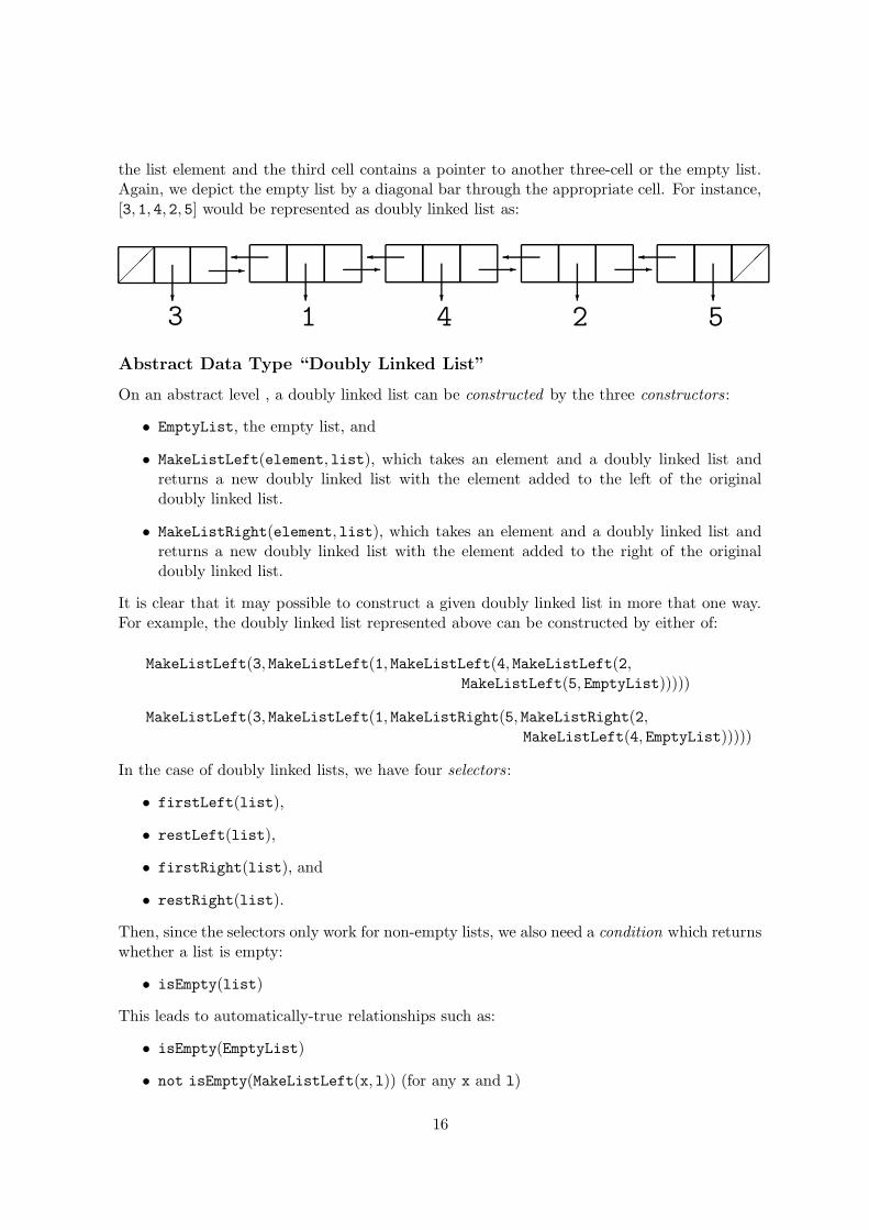
the list element and the third cell contains a pointer to another three-cell or the empty list.Again, we depict the empty list by a diagonal bar through the appropriate cell. For instance,[3, 1, 4, 2, 5] would be represented as doubly linked list as:

���

?

-

3

�

?

-

1

�

?

-

4

�

?

-

2

����

?

5

Abstract Data Type “Doubly Linked List”

On an abstract level , a doubly linked list can be constructed by the three constructors:

• EmptyList, the empty list, and

• MakeListLeft(element, list), which takes an element and a doubly linked list andreturns a new doubly linked list with the element added to the left of the originaldoubly linked list.

• MakeListRight(element, list), which takes an element and a doubly linked list andreturns a new doubly linked list with the element added to the right of the originaldoubly linked list.

It is clear that it may possible to construct a given doubly linked list in more that one way.For example, the doubly linked list represented above can be constructed by either of:

MakeListLeft(3, MakeListLeft(1, MakeListLeft(4, MakeListLeft(2,MakeListLeft(5, EmptyList)))))

MakeListLeft(3, MakeListLeft(1, MakeListRight(5, MakeListRight(2,MakeListLeft(4, EmptyList)))))

In the case of doubly linked lists, we have four selectors:

• firstLeft(list),

• restLeft(list),

• firstRight(list), and

• restRight(list).

Then, since the selectors only work for non-empty lists, we also need a condition which returnswhether a list is empty:

• isEmpty(list)

This leads to automatically-true relationships such as:

• isEmpty(EmptyList)

• not isEmpty(MakeListLeft(x, l)) (for any x and l)

16

• not isEmpty(MakeListRight(x, l)) (for any x and l)

• firstLeft(MakeListLeft(x, l)) = x

• restLeft(MakeListLeft(x, l)) = l

• firstRight(MakeListRight(x, l)) = x

• restRight(MakeListRight(x, l)) = l

Circular Doubly Linked List

As a simple extension of the standard doubly linked list, one can define a circular doublylinked list in which the left-most element points to the right-most element, and vice versa.This is useful when we might need to move efficiently through a whole list of items, but mightnot be starting from one of two particular end points.

2.6 Advantage of Abstract Data Types

It is clear that the implementation of the abstract linked-list data type has the disadvantagethat certain useful procedures may not be directly accessible. For instance, the abstract datatype of a list does not offer a procedure last(l) to give the last element in a list, whereas itwould be trivial to find the last element of an array of a known number of elements. Whilesuch a last procedure can easily be implemented just using the constructors, selectors, andconditions, as we have seen, that may be less efficient than making use of certain aspects ofthe underlying implementation.

That disadvantage leads to an obvious question: Why should we want to use an abstractdata type? Aho, Hopcroft and Ullman (1983) provide a clear answer:

“At first, it may seem tedious writing procedures to govern all accesses to the

underlying structures. However, if we discipline ourselves to writing programs in

terms of the operations for manipulating abstract data types rather than making

use of particular implementations details, then we can modify programs more

readily by reimplementing the operations rather than searching all programs for

places where we have made accesses to the underlying data structures. This

flexibility can be particularly important in large software efforts, and the reader

should not judge the concept by the necessarily tiny examples found in this book.”

This advantage will become clearer when we study more complex abstract data types andalgorithms in later chapters.

17

Chapter 3

Searching

An important and recurring problem in computing is that of locating information. Moresuccinctly, this problem is known as searching . This is a good topic to use for a preliminaryexploration of the various issues involved in algorithm design.

3.1 Requirements for searching

Clearly, the information to be searched has to first be represented (or encoded) somehow.This is where data structures come in. Of course, in a computer, everything is ultimatelyrepresented as sequences of binary digits (bits), but this is too low level for most purposes.What we need to do is develop and study useful data structures which are closer to the wayhumans think, or at least more structured than mere sequences of bits. After all, it is humanswho have to develop and maintain software systems – computers merely run them.

After we have chosen a suitable representation, the represented information has to beprocessed somehow. This is what leads to the need for algorithms. In this case, the processof interest is that of searching. In order to simplify matters, let us assume that we wantto search a collection of integer numbers (though we could equally well deal with strings ofcharacters, or any other data type of interest). To begin with, let us consider:

1. The most obvious and simple representation.

2. Two potential algorithms for processing with that representation.

As we have already noted, arrays are one of the simplest possible ways of representing col-lections of numbers (or strings, or whatever), so we shall use that to store the information tobe searched. Later we shall look at more complex data structures that may make storing andsearching more efficient.

Suppose, for example, that the set of integers we wish to search is {1,4,17,3,90,79,4,6,81}.We can write them in an array a as

a = [1, 4, 17, 3, 90, 79, 4, 6, 81]

If we ask where 17 is in this array, the answer is 2, the index of that element. If we ask where 91is, the answer is nowhere. It is useful to be able to represent nowhere by a number that isnot used as a possible index. Since we start our index counting from 0, any negative numberwould do. We shall follow the convention of using the number −1 to represent nowhere. Other(perhaps better) conventions are possible, but we will stick to this here.

18

3.2 Specification of the search problem

We can now formulate a specification of our search problem using that data structure:

Given an array a and integer x, find an integer i such that

1. if there is no j such that a[j] is x, then i is −1,

2. otherwise, i is any j for which a[j] is x.

The first clause says that if x does not occur in the array a then i should be −1, and thesecond says that if it does occur then i should be a position where it occurs. If there ismore than one position where x occurs, then this specification allows you to return any ofthem – for example, this would be the case if a were [17, 13, 17] and x were 17. Thus, thespecification is ambiguous. Hence different algorithms with different behaviours can satisfythe same specification – for example, one algorithm may return the smallest position atwhich x occurs, and another may return the largest. There is nothing wrong with ambiguousspecifications. In fact, in practice, they occur quite often.

3.3 A simple algorithm: Linear Search

We can conveniently express the simplest possible algorithm in a form of pseudocode whichreads like English, but resembles a computer program without some of the precision or detailthat a computer usually requires:

// This assumes we are given an array a of size n and a key x.

For i = 0,1,...,n-1,

if a[i] is equal to x,

then we have a suitable i and can terminate returning i.

If we reach this point,

then x is not in a and hence we must terminate returning -1.

The ellipsis “. . . ”, for example, is potentially ambiguous, but we, as human beings, knowexactly what is meant here and so we do not need to worry about it. In a programminglanguage such as C or Java, one would write something that is more precise like:

for ( i = 0 ; i < n ; i++ ) {

if ( a[i] == x ) return i;

}

return -1;

In the case of Java, this would be within a method of a class, and more details are needed,such as the parameter a for the method and a declaration of the auxiliary variable i. In thecase of C , this would be within a function, and similar missing details are needed. In either,there would need to be additional code to output the result in a suitable format.

In this case, it is easy to see that the algorithm satisfies the specification (assuming n isthe correct size of the array) – we just have to observe that, because we start counting fromzero, the last position of the array is its size minus one. If we forget this, and let i run from0 to n instead, we get an incorrect algorithm. The practical effect of this mistake is that theexecution of this algorithm gives rise to an error when the item to be located in the array is

19

actually not there, because a non-existing location is attempted to be accessed. Dependingon the particular language, operating system and machine you are using, the actual effect ofthis error will be different. For example, in C running under Unix, you may get executionaborted followed by the message “segmentation fault”, or you may be given the wrong answeras the output. In Java, you will always get an error message.

3.4 A more efficient algorithm: Binary Search

One always needs to consider whether it is possible to improve upon the performance of aparticular algorithm, such as the one we have just created. In the worst case, searching anarray of size n takes n steps. On average, it will take n/2 steps. For a large collection of data,such as the whole world wide web, this will be unacceptable in practice. Thus, we should tryto organize the collection in such a way that a more efficient algorithm is possible. As weshall see later, there are many possibilities, and the more we demand in terms of efficiency,the more complicated the data structures representing the collections tend to become. Herewe shall consider one of the simplest – we still represent the collections by arrays, but now weenumerate the elements in ascending order. The problem of obtaining an ordered list fromany given list is known as sorting and will be studied in detail in a later chapter.

Thus, instead of working with the previous example [1, 4, 17, 3, 90, 79, 4, 6, 81], we wouldwork with [1, 3, 4, 4, 6, 17, 79, 81, 90], which has the same items but listed in ascending order.Then we can use an improved algorithm, which in English-like pseudocode form is:

// This assumes we are given a sorted array a of size n and a key x.

// Use integers left and right (initially set to 0 and n-1) and mid.

While left is less than right,

set mid to the integer part of (left+right)/2, and

if x is greater than a[mid],

then set left to mid+1,

otherwise set right to mid.

If a[left] is equal to x,

then terminate returning left,

otherwise terminate returning -1.

and would correspond to a segment of C or Java code like:

/* DATA */

int a = [1,3,4,4,6,17,79,81,90];

int n = 9;

int x = 79;

/* PROGRAM */

int left = 0, right = n-1, mid;

while ( left < right ) {

mid = ( left + right ) / 2;

if ( x > a[mid] ) left = mid+1;

else right = mid;

}

if ( a[left] == x ) return left;

else return -1;

20

This algorithm works by repeatedly splitting the array into two segments, one going from leftto mid, and the other going from mid + 1 to right, where mid is the position half way fromleft to right, and where, initially, left and right are the leftmost and rightmost positions ofthe array. Because the array is sorted, it is easy to see which of each pair of segments thesearched-for item x is in, and the search can then be restricted to that segment. Moreover,because the size of the sub-array going from locations left to right is halved at each iterationof the while-loop, we only need log2 n steps in either the average or worst case. To see that thisruntime behaviour is a big improvement, in practice, over the earlier linear-search algorithm,notice that log2 1000000 is approximately 20, so that for an array of size 1000000 only 20iterations are needed in the worst case of the binary-search algorithm, whereas 1000000 areneeded in the worst case of the linear-search algorithm.

With the binary search algorithm, it is not so obvious that we have taken proper careof the boundary condition in the while loop. Also, strictly speaking, this algorithm is notcorrect because it does not work for the empty array (that has size zero), but that can easilybe fixed. Apart from that, is it correct? Try to convince yourself that it is, and then try toexplain your argument-for-correctness to a colleague. Having done that, try to write downa convincing argument. Most algorithm developers stop at the first stage, but experienceshows that it is only when we attempt to write down seemingly convincing arguments thatwe actually find all the subtle mistakes.

It is worth considering whether linked-list versions of our two algorithms would work, oroffer any advantages. It is fairly clear that we could perform a linear search through a linkedlist in essentially the same way as with an array, with the relevant pointer returned ratherthan an index. Converting the binary search to linked list form is problematic, because thereis no efficient way to split a linked list into two segments. It seems that our array basedapproach is the best we can do with the data structures we have studied so far.

Notice that we have not yet taken into account how much effort will be required to sortthe array so that the binary search algorithm can work. Until we know that, we cannot besure that the binary search algorithm really is better than the linear search algorithm. Thatmay depend on how many times we need to performa a search on the set of n items – justonce, or as many as n times. We shall return to these issues later. First we need to considerin more detail how to compare algorithm efficiency in a reliable manner.

21

Chapter 4

Efficiency and Complexity

We have already noted that, when developing algorithms, it is important to consider howefficient they are, so we can make informed choices about which are best to use in particularcircumstances. So, before moving on to study increasingly complex data structures andalgorithms, we first look in more deatil at how to measure and describe their efficiency.

4.1 Time versus space complexity

When creating software for serious applications, there is usually a need to judge how quicklyan algorithm or program can complete the given tasks. For example, if you are programminga flight booking system, it will not be considered acceptable if the travel agent and customerhave to wait for half an hour for a transaction to complete. It certainly has to be ensuredthat the waiting time is reasonable for the size of the problem, and normally faster executionis better. We talk about the time complexity of the algorithm as an indicator of how theexecution time depends on the size of the data structure.

Another important efficiency consideration is how much memory a given program willrequire for a particular task, though with modern computers this tends to be less of an issuethan it used to be. Here we talk about the space complexity as how the memory requirementdepends on the size of the data structure.

For a given task, there are often algorithms which trade time for space, and vice versa.For example, we will see that, as a data storage device, hash tables have a very good timecomplexity at the expense of using more memory than is needed by other algorithms. It isusually up to the algorithm/program designer to decide how best to balance the trade-off forthe application they are designing.

4.2 Worst versus average complexity

Another thing that has to be decided when making efficiency considerations is whether it isthe average case performance of an algorithm/program that is important, or whether it ismore important to guarantee that even in the worst case the performance obeys certain rules.For many applications, the average case is more important, because saving time overall isusually more important than guaranteeing good behaviour in the worst case. However, fortime-critical problems (such as keeping track of aeroplanes in certain sectors of air space), itmay be totally unacceptable for the software to take too long if the worst case arises.

22

Again, algorithms/programs often trade-off efficiency of the average case against efficiencyof the worst case. For example, the most efficient algorithm on average might have a par-ticularly bad worst case efficiency. We will see particular examples of this when we considerefficient algorithms for sorting and searching.

4.3 Concrete measures for performance

For the purposes of this module, we will mostly be interested in time complexity . For this,we have to decide how to measure it. Something one might try to do is to just implement thealgorithm and run it, and see how long it takes, but that approachd has a number of pitfalls.For one, if it is a big application and there are several potential algorithms, they would allhave to be programmed first before they can be compared. So a considerable amount of timewould be wasted on writing programs which will not get used in the final product. Also, themachine on which the program is run, or even the compiler used, might influence the runningtime. You would also have to make sure that the data with which you tested your programis typical for the application it is created for. Again, particularly with big applications, thisis not really feasible. This empirical method has another disadvantage: it will not tell youanything useful about the next time you are considering a similar problem.

Therefore complexity is best measured in a different way. Firstly, in order to not bebound to a particular programming language or machine architecture, we typically measurethe efficiency of the algorithm rather than that of its implementation. For this to be possible,however, the algorithm has to be described in a way which very much looks like the program tobe implemented, which is why algorithms are usually best expressed in a form of pseudocodethat come close to the implementation language.

What we need to do to determine the time complexity of an algorithm is count the numberof operations that will occur, which will usually depend on the size of the problem. The sizeof a problem is typically expressed as an integer, and that is typically the number of itemsthat are manipulated. For example, when describing a search algorithm, it is the numberof items amongst which we are searching, and when describing a sorting algorithm, it is thenumber of items to be sorted. So the complexity of an algorithm will be given by a functionwhich maps the number of items to the (usually approximate) number of steps the algorithmwill take when performed on that many items. Because we often have to approximate suchnumbers, and consider averages, we do not demand that the complexity function give us aninteger as the result. Instead we tend to use real numbers for that.

In the early days of computers, operations were counted according to their ‘cost’, withmultiplication of integers typically considered much more expensive than their addition. Intoday’s world, where computers have become much faster, and often have dedicated floating-point hardware, these differences have become less important. But still we need to be carefulwhen deciding to consider all operations equally costly – applying some function, for example,can take longer than adding two numbers (sometimes considerably longer).

4.4 Big-O notation for complexity class

Very often, we are not interested in the actual function C(n) that describes the time complex-ity of an algorithm in terms of the problem size n, but just its complexity class. This ignoresany constant overheads and small constant factors, and just tells us about the principal growth

23

of the complexity function with problem size, and hence something about the performance ofthe algorithm on large numbers of items.

If an algorithm is such that we may consider all steps equally costly, then usually thecomplexity class of the algorithm is simply determined by the number of loops and how oftenthe content of those loops are being executed. The reason for this is that adding a constantnumber of instructions which does not change with the size of the problem has no significanteffect on the overall complexity for large problems.

There is a standard notation, called the Big-O notation, for expressing the fact thatconstant factors and other insignificant details are being ignored. For example, we saw thatthe procedure last(l) on a list l had time complexity that depended linearly on the size nof the list, so we would say that the time complexity of that algorithm is O(n). Similarly,linear search is O(n). For binary search, however, the time complexity is O(log2 n).

Before we define complexity classes in a more formal manner, it is worth trying to gainsome intuition about what they actually mean. For this purpose, it is useful to choose onefunction as a representative of each of the classes we wish to consider. Recall that we areconsidering functions which map natural numbers (the size of the problem) to the set of non-negative real numbers R

+, so the classes will correspond to common mathematical functionssuch as powers and logarithms. We shall consider later to what degree a representative canbe considered ‘typical’ for its class.

The most common complexity classes (in increasing order) are the following:

• O(1), pronounced ‘Oh of one’, or constant complexity;

• O(log2 log2 n), ‘Oh of log log en’;

• O(log2 n), ‘Oh of log en’, or logarithmic complexity;

• O(n), ‘Oh of en’, or linear complexity;

• O(nlog2 n), ‘Oh of en log en’;

• O(n2), ‘Oh of en squared’, or quadratic complexity;

• O(n3), ‘Oh of en cubed’, or cubic complexity;

• O(2n), ‘Oh of two to the en’, or exponential complexity.

As a representative, we choose the function which gives the class its name – e.g. for O(n) wechoose the function f(n) = n, for O(log2 n) we choose f(n) = log2 n, and so on. So assumewe have algorithms with these functions describing their complexity. The following table listshow many operations it will take them to deal with a problem of a given size:

f(n) n = 4 n = 16 n = 256 n = 1024 n = 1048576

1 1 1 1 1.00 × 100 1.00 × 100

log2 log2 n 1 2 3 3.32 × 100 4.32 × 100

log2 n 2 4 8 1.00 × 101 2.00 × 101

n 4 16 2.56 × 102 1.02 × 103 1.05 × 106

nlog2 n 8 64 2.05 × 103 1.02 × 104 2.10 × 107

n2 16 256 6.55 × 104 1.05 × 106 1.10 × 1012

n3 64 4096 1.68 × 107 1.07 × 109 1.15 × 1018

2n 16 65536 1.16 × 1077 1.80 × 10308 6.74 × 10315652

24

Some of these numbers are so large that it is rather difficult to imagine just how long atime span they describe. Hence the following table gives time spans rather than instructioncounts, based on the assumption that we have a computer which can operate at a speed of 1MIP, where one MIP = a million instructions per second:

f(n) n = 4 n = 16 n = 256 n = 1024 n = 1048576

1 1 µsec 1 µsec 1 µsec 1 µsec 1 µseclog2 log2 n 1 µsec 2 µsec 3 µsec 3.32 µsec 4.32 µsec

log2 n 2 µsec 4 µsec 8 µsec 10 µsec 20 µsecn 4 µsec 16 µsec 256 µsec 1.02 msec 1.05 sec

nlog2 n 8 µsec 64 µsec 2.05 msec 1.02 msec 21 secn2 16 µsec 256 µsec 65.5 msec 1.05 sec 1.8 wkn3 64 µsec 4.1 msec 16.8 sec 17.9 min 36, 559 yr2n 16 µsec 65.5 msec 3.7 × 1063 yr 5.7 × 10294 yr 2.1 × 10315639 yr

It is clear that, as the sizes of the problems get really big, there can be huge differencesin the time it takes to run algorithms from different complexity classes. For algorithmswith exponential complexity, O(2n), even modest sized problems have run times that aregreater than the age of the universe (about 1.4 × 1010 yr), and current computers rarely rununinterrupted for more than a few years. This is why complexity classes are so important –they tell us how feasible it is likely to be to run a program with a particular large numberof data items. Typically, people do not worry much about complexity for sizes below 10, ormaybe 20, but the above numbers make it clear why it is worth thinking about complexityclasses where bigger applications are concerned.

Another useful way of thinking about growth classes involves considering how the computetime will vary if the problem size doubles. The following table shows what happens for thevarious complexity classes:

f(n) If the size of the problem doubles then f(n) will be

1 the same, f(2n) = f(n)log2 log2 n almost the same, log2 (log2 (2n)) = log2 (log2 (n) + 1)

log2 n more by 1 = log2 2, f(2n) = f(n) + 1n twice as big as before, f(2n) = 2f(n)

nlog2 n a bit more than twice as big as before, 2nlog2 (2n) = 2(nlog2 n) + 2nn2 four times as big as before, f(2n) = 4f(n)n3 eight times as big as before, f(2n) = 8f(n)2n the square of what it was before, f(2n) = (f(n))2

This kind of information can be very useful in practice. We can test our program on a problemthat is a half or quarter or one eighth of the full size, and have a good idea of how long wewill have to wait for the full size problem to finish. Moreover, that estimate won’t be affectedby any constant factors ignored in computing the growth class, or the speed of the particularcomputer it is run on.

The following graph plots some of the complexity class functions from the table. Notethat although these functions are only defined on natural numbers, they are drawn as thoughthey were defined for all real numbers, because that makes it easier to take in the informationpresented.

25

10 20 30 40 50 60 70 80 90 1000

10

20

30

40

50

60

70

80

90

100

log n

n

n log n

n2

2n

It is clear from these plots why the non-principal growth terms can be safely ignored whencomputing algorithm complexity.

4.5 Formal definition of complexity classes

We have noted that complexity classes are concerned with growth, and the tables and graphabove have provided an idea of what different behaviours mean when it comes to growth.There we have chosen a representative for each of the complexity classes considered, butwe have not said anything about just how ‘representative’ such an element is. Let us nowconsider a more formal definition of a ‘big O’ class:

Definition. A function g belongs to the complexity class O(f) if there is a number n0 ∈ N

and a constant c > 0 such that for all n ≥ n0, we have that g(n) ≤ c ∗ f(n). We say that thefunction g is ‘eventually smaller’ than the function c ∗ f .

It is not totally obvious what this implies. First, we do not need to know exactly wheng becomes smaller than c ∗ f . We are only interested in the existence of n0 such that,from then on, g is smaller than c ∗ f . Second, we wish to consider the efficiency of analgorithm independently of the speed of the computer that is going to execute it. This iswhy f is multiplied by a constant c. The idea is that when we measure the time of thesteps of a particular algorithm, we are not sure how long each of them takes. By definition,g ∈ O(f) means that eventually (namely beyond the point n0), the growth of g will beat most as much as the growth of c ∗ f . This definition also makes it clear that constantfactors do not change the growth class (or O-class) of a function. Hence C(n) = n2 is inthe same growth class as C(n) = 1/1000000 ∗ n2 or C(n) = 1000000 ∗ n2. So we can writeO(n2) = O(1000000 ∗ n2) = O(1/1000000 ∗ n2). Typically, however, we choose the simplestrepresentative, as we did in the tables above. In this case it is O(n2).

26

The various classes we mentioned above are related as follows:

O(1) ⊆ O(log2 log2 n) ⊆ O(log2 (n)) ⊆ O(n) ⊆ O(nlog2 n) ⊆ O(n2) ⊆ O(n3) ⊆ O(2n)

We only consider the principal growth class, so when adding functions from different growthclasses, their sum will always be in the larger growth class. This allows us to simplify terms.For example, the growth class of C(n) = 500000log2 n+4n2+0.3n+100 can be determined asfollows. The summand with the largest growth class is 4n2 (we say that this is the ‘principalsub-term’ or ‘dominating sub-term’ of the function), and we are allowed to drop constantfactors, so this function is in the class O(n2).

When we say that an algorithm ‘belongs to’ some class O(f), we mean that it is at mostas fast growing as f . We have seen that ‘linear searching’ (where one searches in a collectionof data items which is unsorted) has linear complexity, i.e. it is in growth class O(n). Thisholds for the average case as well as the worst case. The operations needed are comparisonsof the item we are searching for with all the items appearing in the data collection. In theworst case, we have to check all n entries until we find the right one, which means we maken comparisons. On average, however, we will only have to check n/2 entries until we hit thecorrect one, leaving us with n/2 operations. Both those functions, C(n) = n and C(n) = n/2belong to the same complexity class, namely O(n). However, it would be equally correct tosay that the algorithm belongs to O(n2), since that class contains all of O(n). But this wouldbe less informative, and we would not say that an algorithm has quadratic complexity if weknow that, in fact, it is linear. Sometimes it is difficult to be sure what the exact complexityis (as is the case with the famous NP = P problem), in which case one might say that analgorithm is ‘at most’, say, quadratic.

The issue of efficiency and complexity class, and their computation, will be a recurringfeature in all the chapters to come. We shall see that concentrating only on the complex-ity class, rather than exact complexity functions, renders the whole process of consideringefficiency much easier.

27

Chapter 5

Trees

In computer science, a tree is a very general and powerful data structure that resembles areal tree. It consists of an ordered set of linked nodes in a connected graph, in which eachnode has at most one parent node, and zero or more children nodes with a specific order.

5.1 General specification of trees

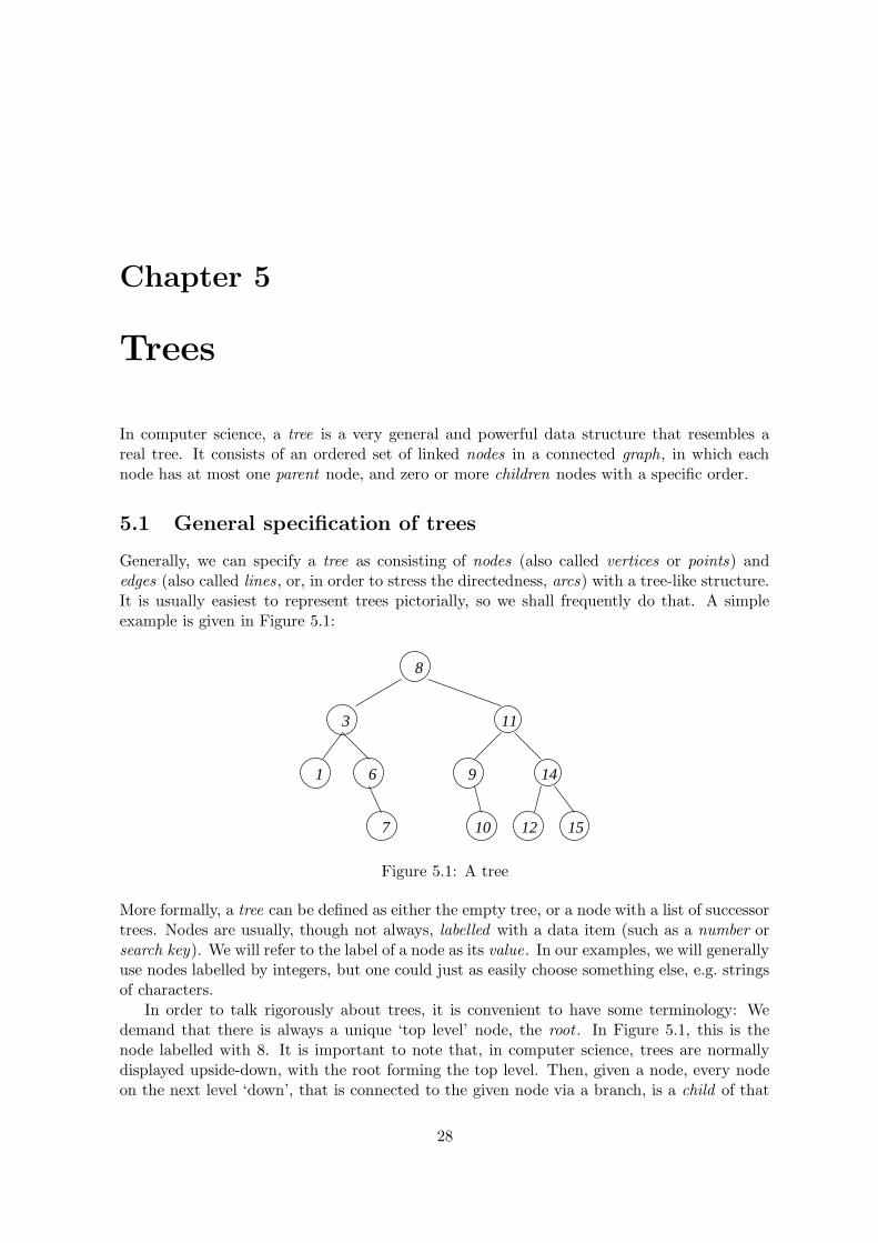
Generally, we can specify a tree as consisting of nodes (also called vertices or points) andedges (also called lines, or, in order to stress the directedness, arcs) with a tree-like structure.It is usually easiest to represent trees pictorially, so we shall frequently do that. A simpleexample is given in Figure 5.1:

10

8

3

1

7

11

9 14

12 15

6

Figure 5.1: A tree

More formally, a tree can be defined as either the empty tree, or a node with a list of successortrees. Nodes are usually, though not always, labelled with a data item (such as a number orsearch key). We will refer to the label of a node as its value. In our examples, we will generallyuse nodes labelled by integers, but one could just as easily choose something else, e.g. stringsof characters.

In order to talk rigorously about trees, it is convenient to have some terminology: Wedemand that there is always a unique ‘top level’ node, the root . In Figure 5.1, this is thenode labelled with 8. It is important to note that, in computer science, trees are normallydisplayed upside-down, with the root forming the top level. Then, given a node, every nodeon the next level ‘down’, that is connected to the given node via a branch, is a child of that

28

node. In Figure 5.1, the children of 8 are 3 and 11. Conversely, the node (there is at mostone) connected to the given node (via an edge) on the level above, is its parent . For instance,11 is the parent of node 9 (and of 14 as well). Nodes that have the same parent are knownas siblings – siblings are, by definition, always on the same level.

If a node is the child of a child of . . . of a another node then we say that the first nodeis a descendent of the second node. Conversely, the second node is an ancestor of the firstnode. Nodes which do not have any children are known as leaves (e.g., the nodes labelledwith 1, 7, 10, 12, and 15 in Figure 5.1).

A path is a sequence of connected edges from one node to another. Trees have the propertythat for every node there is a unique path connecting it with the root. In fact, that is anotherpossible definition of a tree. The depth or level of a node is given by the length of this path.Hence the root has level 0, its children have level 1, and so on. The maximal length of apath in a tree is also called the height of the tree. A path of maximal length always goesfrom the root to a leaf. The size of a tree is given by the number of nodes it contains. Weshall normally assume that every tree is finite, though generally that need not be the case.The tree in Figure 5.1 has height 3 and size 11. A tree consisting of just of one node hasheight 0 and size 1. The empty tree obviously has size 0 and is defined (conveniently, thoughsomewhat artificially) to have height −1.

Like most data structures, we need a set of primitive operators (constructors, selectorsand conditions) to build and manipulate the trees. The details of those depend on the typeand purpose of the tree. We will now look at some particularly useful types of tree.

5.2 Quad-trees

A quadtree is a particular type of tree in which each leaf-node is labelled by a value and eachnon-leaf node has exactly four children. It is used most often to partition a two dimensionalspace (e.g., a pixelated image) by recursively dividing it into four quadrants.

Formally, a quadtree can be defined to be either a single node with a number or value(e.g., in the range 0 to 255), or a node without a value but with four quadtree children: lu,ll, ru, and rl. It can thus be defined “inductively” by the following rules:

Definition. A quad tree is either

(Rule 1) a root node with a value, or

(Rule 2) a root node without a value and four quad tree children: lu, ll, ru, and rl.

Rule 1 is called the “base case” and Rule 2 is called the “induction step”.We say that a quadtree is primitive if it consists of a single node/number, and that can

be tested by the corresponding condition:

• isValue(qt), which returns true if quad-tree qt is a single node.

To build a quad-tree we have two constructors:

• baseQT(value), which returns a single node quad-tree with label value.

• makeQT(luqt, ruqt, llqt, rlqt), which builds a quad-tree from four constituent quad-trees luqt, llqt, ruqt, rlqt.

29

And to extract components from a quad-tree we have four selectors:

• lu(qt), which returns the left-upper quad-tree.

• ru(qt), which returns the right-upper quad-tree.

• ll(qt), which returns the left-lower quad-tree.

• rl(qt), which returns the right-lower quad-tree.

Quad-trees of this type can be used to store grey-value pictures (with 0 representing blackand 255 white). A simple example would be:

10

203040

50 60 70

80110

100

120

90

0

We can then create algorithms using the operators to perform useful manipulations of therepresentation. For example, we could rotate a picture qt by 180◦ using:

rotate(qt) {

if ( isValue(qt) )

return qt

else return makeQT( rotate(rl(qt)), rotate(ll(qt)),

rotate(ru(qt)), rotate(lu(qt)) )

}

There exist variations of this general idea, such edge quad-trees which store lines and allowcurves to be represented with arbitrary precision.

5.3 Binary trees

Binary trees are the most common type of tree used in computer science. A binary tree is atree in which every node has at most two children, and can be defined “inductively” by thefollowing rules:

Definition. A binary tree is either

(Rule 1) the empty tree EmptyTree, or

(Rule 2) it consists of a node and two binary trees, the left subtree and right subtree.

30

Rule 1 is the “base case” and Rule 2 is the “induction step”. This definition may appearcircular, but actually it is not, because the subtrees are always simpler than the original one,and we eventually end up with an empty tree.

You can imagine that the (infinite) collection of (finite) trees is created in a sequence ofdays. Day 0 is when you “get off the ground” by applying Rule 1 to get the empty tree. Onany other day, you are allowed to use the trees that you have created in the previous days,in order to construct new trees using Rule 2. Thus, for example, on day 1 you can createexactly the trees that have a root with a value, but no children (i.e. both the left and rightsubtrees are the empty tree, created at day 0). On day 2 you can use a new node with value,with the empty tree and/or the one-node tree, to create more trees. Thus, binary trees arethe objects created by the above two rules in a finite number of steps. The height of a tree,defined above, is the number of days it takes to create it using the above two rules, where weassume that only one rule is used per day, as we have just discussed. (Exercise: work out thesequence of steps needed to create the tree in Figure 5.1 and hence prove that it is in fact abinary tree.)

5.4 Primitive operations on binary trees

The primitive operators for binary trees are fairly obvious. We have two constructors whichare used to build trees:

• EmptyTree, which returns an empty tree,

• MakeTree(v, l, r), which builds a binary tree from a root node with label v and twoconstituent binary trees l and r,

a condition to test whether a tree is empty:

• isEmpty(t), which returns true if tree t is the EmptyTree,

and three selectors to break a non-empty tree into its constituent parts:

• root(t), which returns the value of the root node of binary tree t,

• left(t), which returns the left sub-tree of binary tree t,

• right(t), which returns the right sub-tree of binary tree t.

These operators can be used to create all the algorithms we might need for manipulatingbinary trees.

For convenience though, it is often a good idea to define derived operators that allow usto write more readable algorithms. For example, we can define a derived constructor:

• Leaf(v) = MakeTree(v, EmptyTree, EmptyTree)

that creates a tree consisting of a single node with label v, which is the root and the uniqueleaf of the tree at the same time. Then the tree in Figure 5.1 can be constructed as:

t = MakeTree(8, MakeTree(3,Leaf(1),MakeTree(6,EmptyTree,Leaf(7))),

MakeTree(11,MakeTree(9,EmptyTree,Leaf(10)),MakeTree(14,Leaf(12),Leaf(15))))

31

which is much simpler than the construction using the primitive operators:

t = MakeTree(8, MakeTree(3,MakeTree(1,EmptyTree,EmptyTree),

MakeTree(6,EmptyTree,MakeTree(7,EmptyTree,EmptyTree))),

MakeTree(11,MakeTree(9,EmptyTree,MakeTree(10,EmptyTree,EmptyTree)),

MakeTree(14,MakeTree(12,EmptyTree,EmptyTree),

MakeTree(15,EmptyTree,EmptyTree))))

Note that the selectors can only operate on non-empty trees. For example, for the tree t

defined above we have

root(left(left(t)) = 1,

but the expression

root(left(left(left(t))))

does not make sense because

left(left(left(t))) = EmptyTree

and the empty tree does not have a root. In a language such as Java, this would typicallyraise an exception. In a language such as C , this would cause an unpredictable behaviour,but if you are lucky, a core dump will be produced and the program will be aborted withno further harm. When writing algorithms, we need to check the selector arguments usingisEmpty(t) before allowing their use.

The following equations should be obvious from the primitive operator definitions:

root(MakeTree(v,l,r)) = v

left(MakeTree(v,l,r)) = l

right(MakeTree(v,l,r)) = r

isEmpty(EmptyTree) = true

isEmpty(MakeTree(v,l,r)) = false

The following makes sense only under the assumption that t is a non-empty tree:

MakeTree(root(t),left(t),right(t)) = t

It just says that if we break apart a non-empty tree and use the pieces to build a new tree,then we get an identical tree back.

It is worth emphasizing that the above specifications of quad-trees and binary trees arefurther examples of abstract data types: Data types for which we exhibit the constructorsand destructors and describe their behaviour (using equations such as defined above for lists,stacks, queues, quad-trees and binary trees), but for which we explicitly hide the implemen-tational details. The concrete data type used in an implementation is called a data structure.For example, the usual data structures used to implement the list and tree data types arerecords and pointers – but other implementations are possible.

The important advantage of abstract data types is that we can develop algorithms withouthaving to worry about the representational details of the data. Of course, everything isultimately represented as sequences of bits in a computer, but we clearly do not generallywant to have to think in such low level terms.

32

5.5 The height of a binary tree

Binary trees don’t have a simple relation between their size n and height h. The maximumheight of a binary tree with n nodes is (n − 1), which happens when all non-leaf nodes haveprecisely one child, forming something that looks like a chain. On the other hand, suppose wehave n nodes and want to build from them a binary tree with minimal height. We can achievethis by ‘filling’ each successive level in turn, starting from the root. It does not matter wherewe place the nodes on the last (bottom) level of the tree, as long as we don’t start adding tothe next level before the previous level is full. Terminology varies, but we shall say that suchtrees are perfectly balanced or height balanced , and we shall see later why they are optimal formany of our purposes. Basically, if done appropriately, many important tree-based operations(such as searching) take as many steps as the height of the tree, so minimizing the heightminimizes the time needed to perform those operations.

We can easily calculate the maximum number of nodes that can fit into a binary tree ofa given height h. Calling this size function s(h), we obtain:

h s(h)

0 11 32 73 15

In fact, it is not difficult to see that s(h) = 1+2+4+ · · ·+2h = 2h+1−1. This can be provedby induction on the definition of a binary tree as follows:

a) The base case applies to the empty tree that has height h = −1, which is consistentwith s(h) = 2−1+1 − 1 = 20 − 1 = 1 − 1 = 0 nodes being stored.

b) Then for the induction step: A tree of height h + 1 has two subtrees of height h, andby the induction hypothesis, each of these subtrees can store s(h) = 2h+1 − 1 nodes. Inaddition, there is the new root which adds an extra node, so all in all a tree of heighth + 1 can have as many as 1 + 2 × (2h+1 − 1) = 1 + 2h+2 − 2 = 2(h+1)+1 − 1 = s(h + 1)nodes, which is what we wanted to show.

An obvious potential problem with inductive proofs like this is the need to find an inductionhypothesis to start with, and that is not always easy.

Another way to proceed here would be to simply sum the series s(h) = 1+2+4+ · · ·+2h

algebraically to get the answer. Sometimes, however, summing the series, or even knowing theseries to be summed, is not so easy. If that is the case, one can try to identify two expressionsfor s(h + 1) as a function of s(h), and then solve them for s(h). Here, a tree of height h + 1is made up of a new node plus two trees of height h, so we can write

s(h + 1) = 1 + 2s(h)

and level h of a tree clearly has 2h nodes, so we can also write:

s(h + 1) = s(h) + 2h+1

Then subtracting one equation from the other gives:

s(h) = 2h+1 − 1

which is the required answer. From this we can get an expression for h

33

h = log2 (s + 1) − 1 ≈ log2 s

in which the approximation is valid for large s.Hence a perfectly balanced tree consisting of n nodes has height approximately log2 n.

This is good, because log2 n is very small, even for relatively large n:

n log2 n

2 132 5

1, 024 101, 048, 576 20

We shall see later how we can use binary trees to hold data in such a way that any search hasat most as many steps as the height of the tree. Therefore, for perfectly balanced trees wecan reduce the search time considerably as the table demonstrates. However, it is not alwayseasy to create perfectly balanced trees, as we shall also see later.

5.6 The size of a binary tree

Usually a binary tree will not be balanced, so we will need an algorithm to determine its size,i.e. the number of nodes it contains. This is easy if we use recursion.

The terminating case is very simple: the empty tree has size 0. Otherwise, since it is abinary tree, it must be assembled from a root node, a left sub-tree left, and a right sub-treeright, and its size will be the sum of the sizes of its components, i.e. 1 for the root, plusthe size of l, plus the size of r. We have already defined the condition isEmpty(t) to checkwhether a binary tree t is empty, and the selectors left(t) and right(t) which return theleft and right sub-trees of binary tree t. Thus we can easily define the procedure size(t),which takes a binary tree t and returns its size, as follows:

size(t) {

if ( isEmpty(t) )

return 0

else return (1 + size(left(t)) + size(right(t)))

}

This recursively processes the whole tree, and we know it will terminate because the treesbeing processed get smaller with each call, and will eventually reach an empty tree whichreturns a simple value.

5.7 Recursive algorithms

Some people have difficulties with recursion. A source of confusion is that it appears that“the algorithm calls itself” and it might therefore get confused about what it is operating on.This way of putting things, although suggestive, can be misleading. The algorithm itself is apassive entity, which actually cannot do anything at all, let alone call itself. What happensis that a processor (which can be a machine or a person) executes the algorithm. So whatgoes on when a processor executes a recursive algorithm such as the one above? An easyway of understanding this is to imagine that whenever a recursive call is encountered, newprocessors are given the task with a copy of the same algorithm.

34

For example, suppose that John (the first processor in this task) wants to compute thesize of a given tree t using the above recursive algorithm. Then, according to the abovealgorithm, John first checks whether it is empty. If it is, he simply returns zero and finisheshis computation. If it isn’t empty, then his tree t must have left and right subtrees l andr (which may, or may not, be empty) and he can extract them using the selectors left(t)and right(t). He can then ask two of his students, say Steve and Mary, to execute thesame algorithm, but for the trees l and r. When they finish, say returning results m andn respectively, he computes and returns 1 + m + n, because his tree has a root node inaddition to the left and right sub-trees. If Steve and Mary aren’t given empty trees, theywill themselves have to delegate executions of the same algorithm, with their sub-trees, toother people. Thus, the algorithm is not calling itself. What happens, is that there are manypeople running their own copies of the same algorithm on different trees.

In this example, in order to make things understandable, we assumed that each personexecutes a single copy of the algorithm. However, the same processor, with some difficulty,can impersonate several processors, in such a way that it achieves the same result as theexecution involving many processors. This is achieved via the use of a stack that keeps trackof the various positions of the same algorithm that are currently being executed – but thisknowledge is not needed for our purposes.

Note that there is nothing to stop us keeping count of the recursions by passing integers,for example:

function(int n, tree t) {

// terminating condition and return

.

// procedure details

.

return function(n-1, t2)

}

so we can do something n times, or look for the nth item, etc. The classic example is therecursive factorial function:

factorial(int n) {

if ( n == 0 ) return 1

return n*factorial(n-1)

}

Often though, we don’t need counters, because there is a particular end point condition, suchas isEmpty(t), that brings the recursion to an end.

35

Chapter 6

Binary Search Trees

We will now look at an important way of storing data that allows us to find a particularitem as quickly as possible. Though, in practice, when efficiency is a crucial factor, furtherelaborations of this way of storing data are used, such as B-trees and AVL trees, at theexpense of requiring more sophisticated algorithms.

6.1 Searching with lists or arrays

As we have already seen in Chapter 3, many computer science applications involve searchingfor a particular item in a collection of data. If the data is stored as an unsorted list or array,then to find the item in question, one obviously has to check each entry in turn until thecorrect one is found, or the collection is exhausted. On average, if there are n items, this willtake n/2 checks, and in the worst case, all n items will have to be checked. If the collection islarge, such as all items accessible via the World Wide Web, that will take too much time. Wealso saw that if the items are sorted before storing in an array, one can perform binary searchwhich only requires log2 n checks in the average and worst cases. The idea here is that, withthe help of binary trees, we can further speed up the storing and search process.

6.2 Search keys

If the items to be searched are labelled via comparable keys, one can order them and storethem in such a way that they are sorted already. Being ‘sorted’ may mean different thingsfor different keys, and which key to choose is an important design decision.

In our examples, the search keys will, for simplicity, usually be integer numbers (such asstudent ID numbers), but other choices occur in practice. For example, the comparable keyscould be words. In that case, comparability usually refers to the alphabetical order. If w andt are words, we write w < t to mean that w precedes t in the alphabetical order. If w = bedand t = sky then the relation w < t holds, but this is not the case if w = bed and t = abacus.A classic example of a collection to be searched is a dictionary. Each entry of the dictionaryis a pair consisting of a word and a definition. The definition is a sequence of words andpunctuation symbols. The search key, in this example, is the word (to which a definitionis attached in the dictionary entry). Thus, abstractly , a dictionary is a sequence of entries,where an entry is a pair consisting of a word and definition. This is what matters from thepoint of view of the search algorithms we are going to consider.

36

Notice the use of the word “abstract”. What we mean is that we abstract or remove anydetails that are irrelevant from the point of view of the algorithms. For example, a dictionaryusually comes in the form of a book, which is a sequence of pages – for us, the distributionof dictionary entries into pages is an accidental feature of the dictionary. All what mattersfor us is that the dictionary is a sequence of entries. So “abstraction” means “getting rid ofirrelevant details”. For our purposes, only the search key is important, and we will ignorethe fact that the entries of the collection will typically be more complex objects (as in theexample of a dictionary or a phone book).

Note that one should always employ the data structure to hold the items which performsbest for the typical application. There is no easy answer as to what the best choice is – theparticular circumstances have to be inspected, and a decision has to be made based on that.However, for many applications, the kind of binary trees we studied in the last chapter areparticularly useful here.

6.3 Binary search trees

The solution to our search problem is to store the collection of data to be searched usinga binary tree in such a way that searching for a particular item takes minimal effort. Theunderlying idea is simple: At each tree node, we want the value of that node to either tell usthat we have found the required item, or tell us which of its two subtrees we should search forit in. For the moment, we shall assume that all the items in the data collection are distinct,so each possible node value occurs at most once. Hence we define:

Definition. A binary search tree is a binary tree that is either empty or satisfies the followingconditions:

• All values occurring in the left subtree are smaller than that of the root.

• All values occurring in the right subtree are larger than that of the root.

• The left and right subtrees are themselves binary search trees.

So this is a special type of binary tree, with node values that are the search keys, and we caninherit many of the operators we defined for general binary trees.

6.4 Building binary search trees

When building a binary search tree, one naturally starts with the root and then adds furthernew nodes as needed. So, to insert a new value v, the following cases arise:

• If the given tree is empty, then simply assign the new value v to the root, and leave theleft and right subtrees empty.

• If the given tree is non-empty, then insert a node with value v as follows:

– If v is equal to the value of the root: report a violated assumption.

– If v is smaller than the value of the root: insert v into the left sub-tree.

– If v is larger than the value of the root: insert v into the right sub-tree.

37

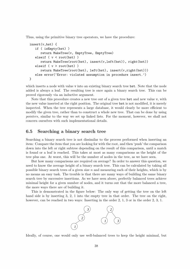
Thus, using the primitive binary tree operators, we have the procedure:

insert(v,bst) {

if ( isEmpty(bst) )

return MakeTree(v, EmptyTree, EmptyTree)

elseif ( v < root(bst) )

return MakeTree(root(bst), insert(v,left(bst)), right(bst))

elseif ( v > root(bst) )

return MakeTree(root(bst), left(bst), insert(v,right(bst)))

else error(‘Error: violated assumption in procedure insert.’)

}

which inserts a node with value v into an existing binary search tree bst. Note that the nodeadded is always a leaf. The resulting tree is once again a binary search tree. This can beproved rigorously via an inductive argument.

Note that this procedure creates a new tree out of a given tree bst and new value v, withthe new value inserted at the right position. The original tree bst is not modified, it is merelyinspected. When the tree represents a large database, it would clearly be more efficient tomodify the given tree, rather than to construct a whole new tree. That can be done by usingpointers, similar to the way we set up linked lists. For the moment, however, we shall notconcern ourselves with such implementational details.

6.5 Searching a binary search tree

Searching a binary search tree is not dissimilar to the process performed when inserting anitem: Compare the item that you are looking for with the root, and then ‘push’ the comparisondown into the left or right subtree depending on the result of this comparison, until a matchis found or a leaf is reached. This takes at most as many comparisons as the height of thetree plus one. At worst, this will be the number of nodes in the tree, as we have seen.

But how many comparisons are required on average? In order to answer this question, weneed to know the average height of a binary search tree. This can be calculated by taking allpossible binary search trees of a given size n and measuring each of their heights, which is byno means an easy task. The trouble is that there are many ways of building the same binarysearch tree by successive insertions. As we have seen above, perfectly balanced trees achieveminimal height for a given number of nodes, and it turns out that the more balanced a tree,the more ways there are of building it.

This is demonstrated in the figure below: The only way of getting the tree on the lefthand side is by inserting 3, 2, 1 into the empty tree in that order. The tree on the right,however, can be reached in two ways: Inserting in the order 2, 1, 3 or in the order 2, 3, 1.

3

1

2

2

1 3

Ideally, of course, one would only use well-balanced trees to keep the height minimal, but

38

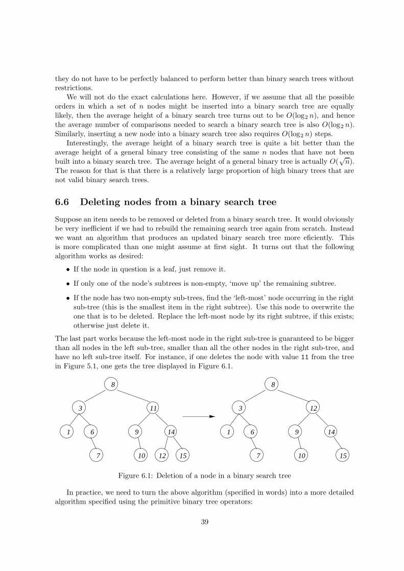
they do not have to be perfectly balanced to perform better than binary search trees withoutrestrictions.

We will not do the exact calculations here. However, if we assume that all the possibleorders in which a set of n nodes might be inserted into a binary search tree are equallylikely, then the average height of a binary search tree turns out to be O(log2 n), and hencethe average number of comparisons needed to search a binary search tree is also O(log2 n).Similarly, inserting a new node into a binary search tree also requires O(log2 n) steps.

Interestingly, the average height of a binary search tree is quite a bit better than theaverage height of a general binary tree consisting of the same n nodes that have not beenbuilt into a binary search tree. The average height of a general binary tree is actually O(

√n).

The reason for that is that there is a relatively large proportion of high binary trees that arenot valid binary search trees.

6.6 Deleting nodes from a binary search tree

Suppose an item needs to be removed or deleted from a binary search tree. It would obviouslybe very inefficient if we had to rebuild the remaining search tree again from scratch. Insteadwe want an algorithm that produces an updated binary search tree more eficiently. Thisis more complicated than one might assume at first sight. It turns out that the followingalgorithm works as desired:

• If the node in question is a leaf, just remove it.

• If only one of the node’s subtrees is non-empty, ‘move up’ the remaining subtree.

• If the node has two non-empty sub-trees, find the ‘left-most’ node occurring in the rightsub-tree (this is the smallest item in the right subtree). Use this node to overwrite theone that is to be deleted. Replace the left-most node by its right subtree, if this exists;otherwise just delete it.

The last part works because the left-most node in the right sub-tree is guaranteed to be biggerthan all nodes in the left sub-tree, smaller than all the other nodes in the right sub-tree, andhave no left sub-tree itself. For instance, if one deletes the node with value 11 from the treein Figure 5.1, one gets the tree displayed in Figure 6.1.

10

8

3

1

7

11

9 14

12 15

6

10

8

3

1

7

9 14

15

6

12

Figure 6.1: Deletion of a node in a binary search tree

In practice, we need to turn the above algorithm (specified in words) into a more detailedalgorithm specified using the primitive binary tree operators:

39

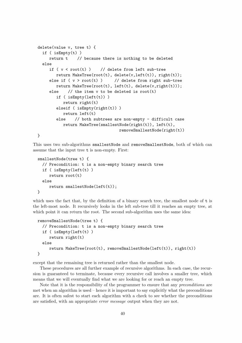
delete(value v, tree t) {

if ( isEmpty(t) )

return t // because there is nothing to be deleted

else

if ( v < root(t) ) // delete from left sub-tree

return MakeTree(root(t), delete(v,left(t)), right(t));

else if ( v > root(t) ) // delete from right sub-tree

return MakeTree(root(t), left(t), delete(v,right(t)));

else // the item v to be deleted is root(t)

if ( isEmpty(left(t)) )

return right(t)

elseif ( isEmpty(right(t)) )

return left(t)

else // both subtrees are non-empty - difficult case

return MakeTree(smallestNode(right(t)), left(t),

removeSmallestNode(right(t))

}

This uses two sub-algorithms smallestNode and removeSmallestNode, both of which canassume that the input tree t is non-empty. First:

smallestNode(tree t) {

// Precondition: t is a non-empty binary search tree

if ( isEmpty(left(t) )

return root(t)

else

return smallestNode(left(t));

}

which uses the fact that, by the definition of a binary search tree, the smallest node of t isthe left-most node. It recursively looks in the left sub-tree till it reaches an empty tree, atwhich point it can return the root. The second sub-algorithm uses the same idea:

removeSmallestNode(tree t) {

// Precondition: t is a non-empty binary search tree

if ( isEmpty(left(t) )

return right(t)

else

return MakeTree(root(t), removeSmallestNode(left(t)), right(t))

}

except that the remaining tree is returned rather than the smallest node.These procedures are all further example of recursive algorithms. In each case, the recur-

sion is guaranteed to terminate, because every recursive call involves a smaller tree, whichmeans that we will eventually find what we are looking for or reach an empty tree.

Note that it is the responsibility of the programmer to ensure that any preconditions aremet when an algorithm is used – hence it is important to say explicitly what the preconditionsare. It is often safest to start each algorithm with a check to see whether the preconditionsare satisfied, with an appropriate error message output when they are not.

40

It is clear from the algorithm that the deletion of a node requires the same number ofsteps as searching for a node, or inserting a new node, i.e. the average height of the binarysearch tree, or O(log2 n) where n is the total number of nodes on the tree.

6.7 Performing a search

Algorithms can be expressed in many ways. Here is a concise description in words of thesearch algorithm that we have already discussed:

In order to search for a value v in a binary search tree t, proceed as follows. If tis empty, then v does not occur in t, and hence we stop with false. Otherwise,if v is equal to the root of t, then v does occur in t, and hence we stop returningtrue. If, on the other hand, v is smaller than the root, then, by definition of abinary search tree, it is enough to search the left sub-tree of t. Hence replace t

by its left sub-tree and carry on in the same way. Similarly, if v is bigger than theroot, replace t by its right sub-tree and carry on in the same way.

Notice that such a description of an algorithm embodies both the steps that need to be carriedout and the reason why this gives a correct solution to the problem. This way of describingalgorithms is very common when we do not intend to run them in a computer.

When we do, we need a more precise specification, such as the pseudocode procedure:

isIn(value v, tree t) {

if ( isEmpty(t) )

return false

elseif ( v == root(t) )

return true

elseif ( v < root(t) )

return isIn(v, left(t))

else

return isIn(v, right(t))

}

Each recursion restricts the search to either the left or right subtree as appropriate, reducingthe search tree height by one, so the algorithm is guaranteed to terminate eventually. In thisexample, the recursion can easily be transformed into a while-loop:

isIn(value v, tree t) {

while ( (not isEmpty(t)) and (v != root(t)) )

if (v < root(t) )

t = left(t)

else

t = right(t)

if ( isEmpty(t) )

return false

else

return true

}

41

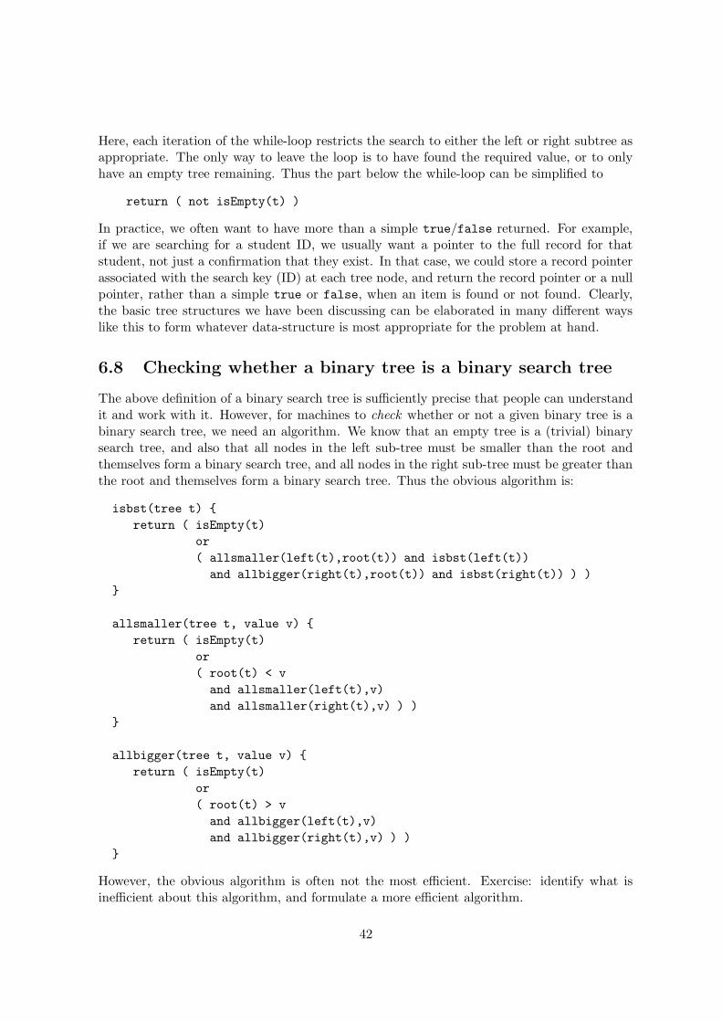
Here, each iteration of the while-loop restricts the search to either the left or right subtree asappropriate. The only way to leave the loop is to have found the required value, or to onlyhave an empty tree remaining. Thus the part below the while-loop can be simplified to

return ( not isEmpty(t) )

In practice, we often want to have more than a simple true/false returned. For example,if we are searching for a student ID, we usually want a pointer to the full record for thatstudent, not just a confirmation that they exist. In that case, we could store a record pointerassociated with the search key (ID) at each tree node, and return the record pointer or a nullpointer, rather than a simple true or false, when an item is found or not found. Clearly,the basic tree structures we have been discussing can be elaborated in many different wayslike this to form whatever data-structure is most appropriate for the problem at hand.

6.8 Checking whether a binary tree is a binary search tree

The above definition of a binary search tree is sufficiently precise that people can understandit and work with it. However, for machines to check whether or not a given binary tree is abinary search tree, we need an algorithm. We know that an empty tree is a (trivial) binarysearch tree, and also that all nodes in the left sub-tree must be smaller than the root andthemselves form a binary search tree, and all nodes in the right sub-tree must be greater thanthe root and themselves form a binary search tree. Thus the obvious algorithm is:

isbst(tree t) {

return ( isEmpty(t)

or

( allsmaller(left(t),root(t)) and isbst(left(t))

and allbigger(right(t),root(t)) and isbst(right(t)) ) )

}

allsmaller(tree t, value v) {

return ( isEmpty(t)

or

( root(t) < v

and allsmaller(left(t),v)

and allsmaller(right(t),v) ) )

}

allbigger(tree t, value v) {

return ( isEmpty(t)

or

( root(t) > v

and allbigger(left(t),v)

and allbigger(right(t),v) ) )

}

However, the obvious algorithm is often not the most efficient. Exercise: identify what isinefficient about this algorithm, and formulate a more efficient algorithm.

42

6.9 Self balancing binary search trees

If the items are added to a binary search tree in random order, the tree tends to be fairlywell balanced with height not much more than log2 n. However, there are many situationswhere the added items are not in random order, such as when adding new student IDs. Inthe extreme case of the new items being added in ascending order, the tree will be one longbranch off to the right, with height n � log2 n.

Self-balancing binary search trees solve this problem by rebalancing the tree from timeto time to keep the height closer to log2 n. Obviously, there will be a cost involved in thatrebalancing, and there will be a trade-off between the time involved in rebalancing and thetime saved by the reduced height of the tree.

The earliest type of self balancing binary search tree was the AVL tree (named after itsinventors G.M. Adelson-Velskii and E.M. Landis). These maintain the difference in heightsof the two sub-trees of all nodes to be at most one. This requires the tree to be periodicallyrebalanced by performing one or more tree rotations, but the complexity of insertion, deletionand search remain at O(log2 n).

Tree rotations can be best understood as follows: Any binary search tree containing atleast two nodes can clearly be drawn in one of the two forms:

where B and D are the required two nodes to be rotated, and A, C and E are binary searchsub-trees (any of which may be empty). The two forms are related by left and right treerotations which clearly preserve the binary search tree property. In this case, any nodes insub-tree A would be shifted up the tree by a right rotation, and any nodes in sub-tree Ewould be shifted up the tree by a left rotation. For example, if the left form had A consistingof two nodes, and C and E consisting of one node, the height of the tree would be reducedby one and become perfectly balanced by a right tree rotation.

Typically, such tree rotations will need to be applied to many different sub-trees of thefull tree to make it perfectly balanced. For example, if the left form had C consisting of twonodes, and A and E consisting of one node, the tree would be balanced by first performing aleft rotation of the A-B-C sub-tree, followed by a right rotation of the whole tree. In practice,finding suitable sequences of appropriate tree rotations to rebalance an arbitrary binary searchtree is not straightforward, but it is possible to formulate systematic algorithms. Exercise:find some suitable algorithms for performing appropriate tree rotations.

6.10 Sorting using binary search trees

Sorting is the process of putting a collection of items in order. We shall formulate and discussmany sorting algorithms later, but we are already able to present one of them.

43

The nodes of a binary search tree can be printed in ascending order by recursively printingeach left sub-tree, root, and right sub-tree in the right order as follows:

printInOrder(tree t) {

if ( not isEmpty(t) ) {

printInOrder(left(t))

print(root(t))

printInOrder(right(t))

}

}

Then, if the collection of items to be sorted is given as an array a of known size n, they canbe printed in sorted order by the algorithm:

sort(array a of size n) {

t = EmptyTree

for i = 0,1,...,n-1

t = insert(a[i],t)

printInOrder(t)

}

which starts with an empty tree, inserts all the items into it using insert(v, t) to give abinary search tree, and then prints them in order using printInOrder(t). Exercise: modifythis algorithm so that instead of printing the sorted values, they are put back into the originalarray in ascending order.

6.11 B-trees

A B-tree is a generalization of a binary search tree in which a node can hold more than onesearch key and have more than two children. The standard (Knuth) definition is:

Definition. A B-tree of order m is a tree which satisfies the following conditions:

• The root node has at least two children if it is not a leaf node.

• Every node (except the root node) has at least m/2 children.

• Every node has at most m children.

• A non-leaf node with c children contains c−1 search keys which act as separation valuesto divide its sub-trees.

• All leaf nodes appear in the same level, and carry information.

The standard representation of simple order 4 example would be:

44

The non-leaf node’s elements act as separation values to divide the contents of its sub-treesin much the same way that a node’s value in a binary search tree separates the values in itstwo sub-trees.

For example, if a node has 3 child nodes (or sub-trees) then it must have 2 separationvalues s1 and s2. All values in the leftmost subtree will be less than s1, all values in themiddle subtree will be between s1 and s2, and all values in the rightmost subtree will begreater than s2. That allows insertion and searching to proceed from the root down in asimilar way to binary search trees.

The restriction on the number of children to lie between m/2 and m means that the bestcase height of an order m B-tree containing n search keys is logmn and the worst case heightis logm/2n. Clearly the costs of insertion, deletion and searching will be proportional to thoseheights, as in a binary search tree.

The order of a B-tree is typically chosen to optimize a particular application and imple-mentation. To maintain the conditions of the B-tree definition, non-leaf nodes often have tobe split or joined when new items are inserted into or deleted from the tree (which is whythere is a factor of two between the minimum and maximum number of children), and thetree often needs rebalancing . This renders the insertion and deletion algorithms somewhatmore complicated than for binary search trees. An advantage of B-trees over self balancingbinary search trees is that the range of child nodes means that rebalancing is required lessfrequently. A disadvantage is that there may be more space wastage because nodes will rarelybe completely full. There is also the need for keeping the items within a node ordered, and tosearch among them, but for reasonably small m that cost is low. Exercise: find some suitableinsertion and deletion algorithms for B-trees.

45

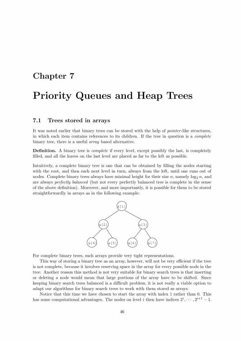
Chapter 7

Priority Queues and Heap Trees

7.1 Trees stored in arrays

It was noted earlier that binary trees can be stored with the help of pointer -like structures,in which each item contains references to its children. If the tree in question is a completebinary tree, there is a useful array based alternative.

Definition. A binary tree is complete if every level, except possibly the last, is completelyfilled, and all the leaves on the last level are placed as far to the left as possible.

Intuitively, a complete binary tree is one that can be obtained by filling the nodes startingwith the root, and then each next level in turn, always from the left, until one runs out ofnodes. Complete binary trees always have minimal height for their size n, namely log2 n, andare always perfectly balanced (but not every perfectly balanced tree is complete in the senseof the above definition). Moreover, and more importantly, it is possible for them to be storedstraightforwardly in arrays as in the following example:

a[4] a[5] a[6] a[7]

a[2] a[3]

a[1]

For complete binary trees, such arrays provide very tight representations.This way of storing a binary tree as an array, however, will not be very efficient if the tree

is not complete, because it involves reserving space in the array for every possible node in thetree. Another reason this method is not very suitable for binary search trees is that insertingor deleting a node would mean that large portions of the array have to be shifted. Sincekeeping binary search trees balanced is a difficult problem, it is not really a viable option toadapt our algorithms for binary search trees to work with them stored as arrays.

Notice that this time we have chosen to start the array with index 1 rather than 0. Thishas some computational advantages. The nodes on level i then have indices 2i, · · · , 2i+1 − 1.

46

The level of a node with index i is blog2 ic, that is, log2 i rounded down. The children of anode with index i, if they exist, have indices 2i and 2i+1. The parent of a child with index ihas index i/2 (using integer division). This allows the following simple algorithms:

boolean isRoot(int i) {

return i == 1

}

int level(int i) {

return log(i)

}

int parent(int i) {

return i / 2

}

int left(int i) {

return 2 * i

}

int right(int i) {

return 2 * i + 1

}

which make the processing of these trees much easier.

7.2 Priority queues and binary heap trees

While most queues in every-day life operate on a first come, first served basis, it is sometimesimportant to be able to assign a priority to the items in the queue, and always serve the itemwith the highest priority next. An example of this would be in a hospital casualty department,where life-threatening injuries need to be treated first. The structure of a complete binarytree is particularly useful for representing such a priority queue.

It turns out that these queues can be implemented efficiently by a particular type ofbinary tree known as a binary heap tree. The idea is that the node labels, which used to bethe search keys when we were talking about binary search trees, are now numbers representingthe priority of the item in question (with higher numbers meaning a higher priority in ourexamples). With heap tress it is possible to insert and remove elements efficiently withouthaving to keep it sorted like a binary search tree. This is because we only ever want to removeone element at a time, namely the one with the highest priority present, and the idea is thatthe highest priority item will always be found at the root of the tree.

Definition. A binary heap tree is a complete binary tree which is either empty or satisfiesthe following conditions:

• The priority of the root is higher than (or equal to) that of its children.

• The left and right subtrees of the root are heap trees.

47

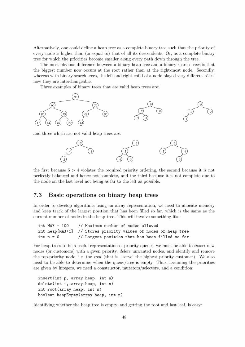
Alternatively, one could define a heap tree as a complete binary tree such that the priority ofevery node is higher than (or equal to) that of all its descendents. Or, as a complete binarytree for which the priorities become smaller along every path down through the tree.

The most obvious difference between a binary heap tree and a binary search trees is thatthe biggest number now occurs at the root rather than at the right-most node. Secondly,whereas with binary search trees, the left and right child of a node played very different roles,now they are interchangeable.

Three examples of binary trees that are valid heap trees are:

14

42 60

70

75

96

17 1044 72

80

90 9

8 8

1 3

9

3 2

1

and three which are not valid heap trees are:

6

5 4

3

6

5

4 3

6

5

4 3

the first because 5 > 4 violates the required priority ordering, the second because it is notperfectly balanced and hence not complete, and the third because it is not complete due tothe node on the last level not being as far to the left as possible.

7.3 Basic operations on binary heap trees

In order to develop algorithms using an array representation, we need to allocate memoryand keep track of the largest position that has been filled so far, which is the same as thecurrent number of nodes in the heap tree. This will involve something like:

int MAX = 100 // Maximum number of nodes allowed

int heap[MAX+1] // Stores priority values of nodes of heap tree

int n = 0 // Largest position that has been filled so far

For heap trees to be a useful representation of priority queues, we must be able to insert newnodes (or customers) with a given priority, delete unwanted nodes, and identify and removethe top-priority node, i.e. the root (that is, ‘serve’ the highest priority customer). We alsoneed to be able to determine when the queue/tree is empty. Thus, assuming the prioritiesare given by integers, we need a constructor, mutators/selectors, and a condition:

insert(int p, array heap, int n)

delete(int i, array heap, int n)

int root(array heap, int n)

boolean heapEmpty(array heap, int n)

Identifying whether the heap tree is empty, and getting the root and last leaf, is easy:

48

boolean heapEmpty(array heap, int n) {

return n == 0

}

int root(array heap, int n) {

if ( heapEmpty(heap,n) )

error(‘Heap is empty’)

else return heap[1]

}

int lastLeaf(array heap, int n) {

if ( heapEmpty(heap,n) )

error(‘Heap is empty’)

else return heap[n]

}

Inserting and deleting heap tree nodes is also straightforward, but not quite so easy.

7.4 Inserting a new heap tree node

Since we always keep track of the last position n in the tree which has been filled so far, wecan easily insert a new element at position n + 1, provided there is still room in the array,and increment n. The tree that results will still be a complete binary tree, but the heap treepriority ordering property might have been violated. Hence we may need to ‘bubble up’ thenew element into a valid position. This can be done easily by comparing its priority withthat of its parent, and if the new element has higher priority, then it is exchanged with itsparent. We may have to repeat this process, but once we reach a parent that has higher orequal priority, we can stop because we know there can be no lower priority items further upthe tree. Hence an algorithm which inserts a new heap tree node with priority p is:

insert(int p, array heap, int n) {

if ( n == MAX ) {

error(‘Heap is full’)

else {

heap[n+1] = p

bubbleUp(n+1,heap,n+1)

}

}

bubbleUp(int i, array heap, int n) {

if ( isRoot(i) )

return

elseif ( heap[i] > heap[parent(i)] ) {

swap heap[i] and heap[parent(i)]

bubbleUp(parent(i),heap,n)

}

}

49

Note that this insert algorithm does not increment the heap size n – that has to be doneseparately by whatever algorithm calls it.

Inserting a node takes at most O(log2 n) steps, because the maximum number of timeswe may have to ‘bubble up’ the new element is the height of the tree which is log2 n.

7.5 Deleting a heap tree node

To use a binary heap tree as a priority queue, we will regularly need to delete the root, i.e.remove the node with the highest priority. We will then be left with something which is not abinary tree at all. However, we can easily make it into a complete binary tree again by takingthe node at the ‘last’ position and using that to fill the new vacancy at the root. However, aswith insertion of a new item, the heap tree (priority ordering) property might be violated. Inthat case, we will need to ‘bubble down’ the new root by comparing it with both its childrenand exchanging it for the largest. This process is then repeated until the new root elementhas found a valid place. Thus, a suitable algorithm is:

deleteRoot(array heap, int n) {

if ( n < 1 )

error(‘Node does not exist’)

else {

heap[1] = heap[n]

bubbleDown(1,heap,n-1)

}

}

A similar process can also be applied if we need to delete any other node from the heap tree,but in that case we may need to ‘bubble up’ the shifted last node rather than bubble it down.Since the original heap tree is ordered, items will only ever need to be bubbled up or down,never both, so we can simply call both, because neither procedure changes anything if it isnot required. Thus, an algorithm which deletes any node i from a heap tree is:

delete(int i, array heap, int n) {

if ( n < i )

error(‘Node does not exist’)

else {

heap[i] = heap[n]

bubbleUp(i,heap,n-1)

bubbleDown(i,heap,n-1)

}

}

The bubble down process is more difficult to implement than bubble up, because a nodemay have none, one or two children, and those three cases have to be handled differently. Inthe case of two children, it is crucial that when both children have higher priority than thegiven node, it is the highest priority one that is swapped up, or their priority ordering willbe violated. Thus we have:

50

bubbleleDown(int i, array heap, int n) {

if ( left(i) > n ) // no children

return

elseif ( right(i) > n ) // only left child

if ( heap[i] < heap[left(i)] )

swap heap[i] and heap[left(i)]

else // two children

if ( heap[left(i)] > heap[right(i)] and heap[i] < heap[left(i)] ) {

swap heap[i] and heap[left(i)]

bubbleDown(left(i),heap,n)

}

elseif ( heap[i] < heap[right(i)] ) {

swap heap[i] and heap[right(i)]

bubbleDown(right(i),heap,n)

}

}

}

In the same way that the insert algorithm does not increment the heap size, this delete

algorithm does not decrement the heap size n – that has to be done separately by whateveralgorithm calls it. Note also that this algorithm does not attempt to be fair in the sense thatif two or more nodes have the same priority, it is not necessarily the one that has been waitinglongest that will be removed first. However, this factor could easily be fixed, if required, bykeeping track of arrival times and using that in cases of equal priority.

As with insertion, deletion takes at most O(log2 n) steps, because the maximum numberof times it may have to bubble down or bubble up the replacement element is the height ofthe tree which is log2 n.

7.6 Building a new heap tree

Sometimes one is given a whole set of n new items in one go, and there is a need to builda binary heap tree containing them. In other words, we have a set of items that we wishto heapify . One obvious possibility would be to insert the n items one by one into a heaptree, starting from an empty tree, using the O(log2 n) ‘bubble up’ based insert algorithmdiscussed earlier. That would clearly have overall time complexity of O(nlog2 n).

It turns out, however, that rearranging an array of items into heap tree form can be donemore efficiently using ‘bubble down’. First note that, if we have the n items in an array a inpositions 1, . . . , n, then all the items with an index greater than n/2 will be leaves, and notneed bubbling down. Therefore, if we just bubble down all the non-leaf items a[n/2],...,

a[1] by exchanging them with the larger of their children until they either are positioned ata leaf, or until their children are both smaller, we obtain a valid heap tree.

Consider a simple example array if items from which a heap tree must be built:

5 8 3 9 1 4 7 6 2

We can start by simply drawing the array as a tree, and see that the last 5 entries (those withindices greater than 9/2 = 4) are leaves of the tree, as follows:

51

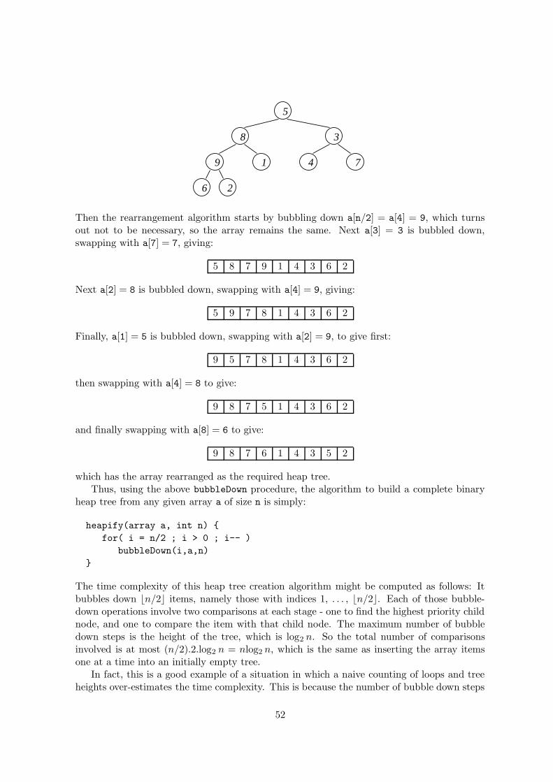
9

6 2

1 4 7

8 3

5

Then the rearrangement algorithm starts by bubbling down a[n/2] = a[4] = 9, which turnsout not to be necessary, so the array remains the same. Next a[3] = 3 is bubbled down,swapping with a[7] = 7, giving:

5 8 7 9 1 4 3 6 2

Next a[2] = 8 is bubbled down, swapping with a[4] = 9, giving:

5 9 7 8 1 4 3 6 2

Finally, a[1] = 5 is bubbled down, swapping with a[2] = 9, to give first:

9 5 7 8 1 4 3 6 2

then swapping with a[4] = 8 to give:

9 8 7 5 1 4 3 6 2

and finally swapping with a[8] = 6 to give:

9 8 7 6 1 4 3 5 2

which has the array rearranged as the required heap tree.Thus, using the above bubbleDown procedure, the algorithm to build a complete binary

heap tree from any given array a of size n is simply:

heapify(array a, int n) {

for( i = n/2 ; i > 0 ; i-- )

bubbleDown(i,a,n)

}

The time complexity of this heap tree creation algorithm might be computed as follows: Itbubbles down bn/2c items, namely those with indices 1, . . . , bn/2c. Each of those bubble-down operations involve two comparisons at each stage - one to find the highest priority childnode, and one to compare the item with that child node. The maximum number of bubbledown steps is the height of the tree, which is log2 n. So the total number of comparisonsinvolved is at most (n/2).2.log2 n = nlog2 n, which is the same as inserting the array itemsone at a time into an initially empty tree.

In fact, this is a good example of a situation in which a naive counting of loops and treeheights over-estimates the time complexity. This is because the number of bubble down steps

52

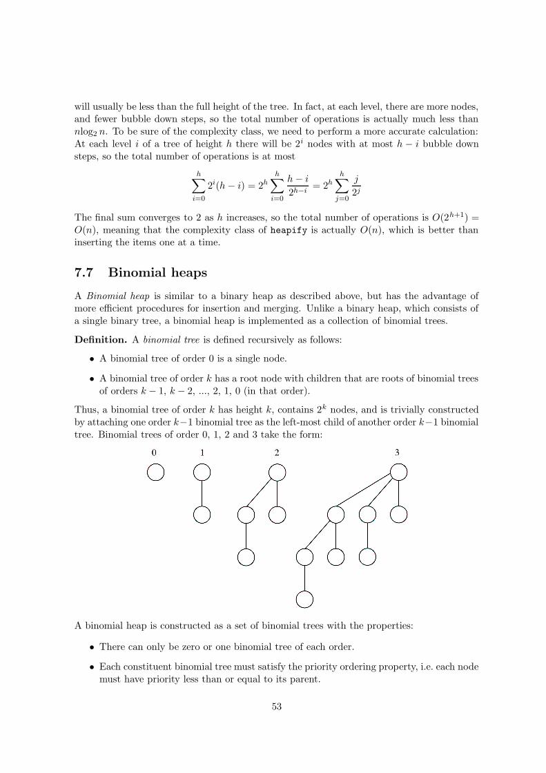
will usually be less than the full height of the tree. In fact, at each level, there are more nodes,and fewer bubble down steps, so the total number of operations is actually much less thannlog2 n. To be sure of the complexity class, we need to perform a more accurate calculation:At each level i of a tree of height h there will be 2i nodes with at most h − i bubble downsteps, so the total number of operations is at most

h∑

i=0

2i(h − i) = 2hh

∑

i=0

h − i

2h−i= 2h

h∑

j=0

j

2j

The final sum converges to 2 as h increases, so the total number of operations is O(2h+1) =O(n), meaning that the complexity class of heapify is actually O(n), which is better thaninserting the items one at a time.

7.7 Binomial heaps

A Binomial heap is similar to a binary heap as described above, but has the advantage ofmore efficient procedures for insertion and merging. Unlike a binary heap, which consists ofa single binary tree, a binomial heap is implemented as a collection of binomial trees.

Definition. A binomial tree is defined recursively as follows:

• A binomial tree of order 0 is a single node.

• A binomial tree of order k has a root node with children that are roots of binomial treesof orders k − 1, k − 2, ..., 2, 1, 0 (in that order).

Thus, a binomial tree of order k has height k, contains 2k nodes, and is trivially constructedby attaching one order k−1 binomial tree as the left-most child of another order k−1 binomialtree. Binomial trees of order 0, 1, 2 and 3 take the form:

A binomial heap is constructed as a set of binomial trees with the properties:

• There can only be zero or one binomial tree of each order.

• Each constituent binomial tree must satisfy the priority ordering property, i.e. each nodemust have priority less than or equal to its parent.

53

The heap structure for n nodes is unique, and will consist of at most log2 n + 1 trees. Thehighest priority node in the heap is the highest priority root node, and a pointer to that caneasily be maintained by each heap update operation. Exercise: find out how the insert, deleteand merge algorithms work for binomial heaps, and compare their time complexities to thoseof standard binary heaps.

7.8 Fibonacci heaps

A Fibonacci heap is another collection of trees satisfying the standard heap property, namelythat the priority of a child is always less than or equal to that of the parent. Thus it canbe used as a priority queue in a similar way to a standard binary or binomial heap, but thestructure of a Fibonacci heap is more flexible and efficient, and has better run times thanbinary and binomial heaps. This flexibility and efficiency, however, comes at the cost of morecomplexity: the trees do not have a fixed shape, and in the extreme cases every element inthe heap can be in a separate tree.

For each node, a record is kept of its number of children and whether it is marked. Fastdeletion and merging are made possible by having the roots of all the trees linked using acircular doubly linked list , and the children of each node are also linked in the same manner.This means heap merging can be accomplished in constant time by simply concatenating thelists of the roots, and insertion can be done by merging with a new heap consisting only ofthe new node. A pointer to the highest priority root node is maintained, making it trivial tofind the highest priority node in the heap.

Fibonacci heaps are important in practice because they are used in the most efficientversions of many algorithms that can be implemented using a priority queue. Exercise: findout how the various Fibonacci heap operations work, and compare their time complexities tothose of binary and binomial heaps.

54

Chapter 8

Sorting

8.1 The problem of sorting

In computer science, ‘sorting’ usually refers to bringing a set of items into some well-definedorder. To be able to do this, we first need to specify the notion of order on the items we areconsidering. For example, for numbers we can use the usual numerical order (that is, definedby the mathematical ‘less than’ or ‘<’ relation) and for strings the so-called lexicographic oralphabetic order, which is the one dictionaries and encyclopedias use.

Usually, what is meant by sorting is that once the sorting process is finished, there isa simple way of ‘visiting’ all the items in order, for example to print out the contents of adatabase. This may well mean different things depending on how the data is being stored.For example, if all the objects are sorted and stored in an array a of size n, then

for i = 0,...,n-1

print(a[i])

would print the items in ascending order. If the objects are stored in a linked list, we wouldexpect that the first entry is the smallest, the next the second-smallest, and so on. Often,more complicated structures such as binary search trees or heap trees are used to sort theitems, which can then be printed, or written into an array or linked list, as desired.

Sorting is important because having the items in order makes it much easier to find a givenitem, such as the cheapest item or the file corresponding to a particular student. It is thusclosely related to the problem of search, as we saw with the discussion of binary search tress.If the sorting can be done beforehand (off-line), this enables faster access to the requireditem, which is important because that often has to be done on the fly (on-line). We havealready seen that, by having the data items stored in a sorted array or binary search tree,we can reduce the average (and worst case) complexity of searching for a particular item toO(log2 n) steps, whereas it would be O(n) steps without sorting. So, if we often have to lookup items, it is worth the effort to sort the whole collection first. Imagine using a dictionaryor phone book in which the entries do not appear in some known logical order.

It follows that sorting algorithms are important tools for program designers. Differentalgorithms are suited to different situations, and we shall see that there is no ‘best’ sortingalgorithm for everything, and therefore a number of them will be introduced in this module.It is worth noting that we will be far from covering all existing sorting algorithms – in fact,the field is still very much alive, and new developments are taking place all the time. However,

55

the general strategies can now be considered to be well-understood, and most of the latestnew algorithms tend to be derived by simply tweaking existing principles, although we stilldo not have accurate measures of performance for some sorting algorithms.

8.2 Common sorting strategies

One way of organizing the various sorting algorithms is by classifying the underlying idea, or‘strategy’. Some of the key strategies are:

enumeration sorting Consider all items. If we know that there are N items which aresmaller than the one we are currently considering, then its finalposition will be at number N + 1.

exchange sorting If two items are found to be out of order, exchange them. Repeattill all items are in order.

selection sorting Find the smallest item, put it in the first position, find the smallestof the remaining items, put it in the second position . . .

insertion sorting Take the items one at a time and insert them into an initiallyempty data structure such that the data structure continues tobe sorted at each stage.

divide and conquer Recursively split the problem into smaller sub-problems till youjust have single items that are trivial to sort. Then put the sorted‘parts’ back together in a way that preserves the sorting.

All these strategies are based on comparing items and then rearranging them accordingly.These are known as comparison-based sorting algorithms. We will later consider other non-comparison-based algorithms which are possible when we have specific prior knowledge aboutthe items that can occur, or restrictions on the range of items that can occur.

The ideas above are based on the assumption that all the items to be sorted will fit intothe computer’s internal memory, which is why they are often referred to as being internalsorting algorithms. If the whole set of items cannot be stored in the internal memory at onetime, different techniques have to be used. These days, given the growing power and memoryof computers, external storing devices are becoming much less commonly used when sorting,so we will not consider external sorting algorithms in detail. Suffice to say, they generallywork by splitting the set of items into subsets containing as many items as can be handled atone time, sorting each subset in turn, and then carefully merging the results.

8.3 How many comparisons must it take?

An obvious way to judge the time complexity of sorting algorithms is to count the number ofcomparisons they need to carry out, as a function of the number of items to be sorted. Thereis clearly no general upper bound on the number of comparisons used, since a particularlystupid algorithm might compare the same two items indefinitely. We are more interested inhaving a lower bound for the number of comparisons needed for the best algorithm in theworst case. In other words, we want to know the minimum number of comparisons required

56

to have all the information needed to sort an arbitrary collection of items. Then we can seehow well particular sorting algorithms compare against that theoretical lower bound.

In general, questions of this kind are rather hard, because of the need to consider allpossible algorithms. In fact, for some problems, optimal lower bounds are not yet known.One important example is the so-called Travelling Salesman Problem (TSP), for which allalgorithms, which are known to give the correct shortest route solution, are extremely inef-ficient in the worst case (many to the extent of being useless in practice). In these cases,one generally has to relax the problem to find solutions which are probably approximatelycorrect. For the TSP, it is still an open problem whether there exists a feasible algorithmthat is guaranteed to give the exact shortest route.

For sorting algorithms based on comparisons, however, it turns out that a tight lowerbound does exist. Clearly, even if the given collection of items is already sorted, we must stillcheck all the items one at a time to see whether they are in the correct order. Thus, the lowerbound must be at least n, the number of items to be sorted, since we need at least n steps toexamine every element. If we already knew a sorting algorithm that works in n steps, thenwe could stop looking for a better algorithm: n would be both a lower bound and an upperbound to the minimum number of steps, and hence an exact bound . However, as we shallshortly see, no algorithm can actually take fewer than O(nlog2 n) comparisons in the worstcase. If, in addition, we can design an algorithm that works in O(nlog2 n) steps, then we willhave obtained an exact bound. We shall start by demonstrating that every algorithm needsat least nlog2 n comparisons.

To begin with, let us assume that we only have three items, i, j, and k. If we have foundthat i ≤ j and j ≤ k, then we know that the sorted order is: i, j, k. So it took us twocomparisons to find this out. In some cases, however, it is clear that we will need as many asthree comparisons. For example, if the first two comparisons tell us that i > j and j ≤ k, thenwe know that j is the smallest of the three items, but we cannot say from this informationhow i and k relate. A third comparison is needed. So what is the average and worst numberof comparisons that are needed? This can best be determined from the so-called decision tree,where we keep track of the information gathered so far and count the number of comparisonsneeded. The decision tree for the three item example we were discussing is:

i <= k

j <= k

j <= k

i <= k

i <= j

k <= i <= ji <= k <= j

i <= j <= k j <= i <= k

k <= j <= ij <= k <= i

yes

yes no yes no

noyes no yes

no

So what can we deduce from this about the general case? The decision tree will obviouslyalways be a binary tree. It is also clear that its height will tell us how many comparisons willbe needed in the worst case, and that the average length of a path from the root to a leafwill give us the average number of comparisons required. The leaves of the decision tree are

57

all the possible outcomes. These are given by the different possible orders we can have on nitems, so we are asking how many ways there are of arranging n items. The first item canbe any of the n items, the second can be any of the remaining n − 1 items, and so forth, sotheir total number is n(n − 1)(n − 2) · · · 3 · 2 · 1 = n!. Thus we want to know the height h ofa binary tree that can accommodate as many as n! leaves. The number of leaves of a tree ofheight h is at most 2h, so we want to find h such that

2h ≥ n! or h ≥ log2 (n!)

There are numerous approximate expressions that have been derived for log2 (n!) for large n,but they all have the same dominant term, namely nlog2 n. (Remember that, when talkingabout time complexity, we ignore any sub-dominant terns and constant factors.) Hence,no sorting algorithm based on comparing items can have a better average or worst caseperformance than using a number of comparisons that is approximately nlog2 n. It remainsto be seen whether this O(nlog2 n) complexity can actually be achieved in practice. To dothis, we would have to exhibit at least one algorithm with this performance behaviour (andconvince ourselves that it really does have this behaviour). In fact, we shall shortly see thatthere are several algorithms with this behaviour.

We shall proceed by looking in turn at a number of sorting algorithms of increasingsophistication, that involve the various strategies listed above. The way they work dependson what kind of data structure contains the items we wish to sort. We start with approachesthat work with simple arrays, and then move on to using more complex data structures thatlead to more efficient algorithms.

8.4 Bubble Sort

Bubble Sort follows the exchange sort approach. It is very easy to implement, but tends tobe particularly slow to run. Assume we have array a of size n that we wish to sort. BubbleSort starts by comparing a[n-1] with a[n-2] and swaps them if they are in the wrong order.It then compares a[n-2] and a[n-3] and swaps those if need be, and so on. This meansthat once it reaches a[0], the smallest entry will be in the correct place. It then starts fromthe back again, comparing pairs of ‘neighbours’, but leaving the zeroth entry alone (which isknown to be correct). After it has reached the front again, the second-smallest entry will bein place. It keeps making ‘passes’ over the array until it is sorted. More generally, at the ithstage Bubble Sort compares neighbouring entries ‘from the back’, swapping them as needed.The item with the lowest index that is compared to its right neighbour is a[i-1]. After theith stage, the entries a[0],...,a[i-1] are in their final position.

At this point it is worth introducing a simple ‘test-case’ of size n = 4 to demonstrate howthe various sorting algorithms work:

4 1 3 2

Bubble Sort starts by comparing a[3]=2 with a[2]=3. Since they are not in order, it swapsthem, giving 4 1 2 3 . It then compares a[2]=2 with a[1]=1. Since those are in order,it leaves them where they are. Then it compares a[1]=1 with a[0]=1, and those are not inorder once again, so they have to be swapped. We get 1 4 2 3 . Note that the smallestentry has reached its final place. This will always happen after Bubble Sort has done its first‘pass’ over the array.

58

Now that the algorithm has reached the zeroth entry, it starts at the back again, comparinga[3]=3 with a[2]=2. These entries are in order, so nothing happens. (Note that thesenumbers have been compared before – there is nothing in Bubble Sort that prevents it fromrepeating comparisons, which is why it tends to be pretty slow!) Then it compares a[2]=2

and a[1]=4. These are not in order, so they have to be swapped, giving 1 2 4 3 . Sincewe already know that a[0] contains the smallest item, we leave it alone, and the second passis finished. Note that now the second-smallest entry is in place, too.

The algorithm now starts the third and final pass, comparing a[3]=3 and a[2]=4. Againthese are out of order and have to be swapped, giving 1 2 3 4 . Since it is known thata[0] and a[1] contain the correct items already, they are not touched. Furthermore, thethird-smallest item is in place now, which means that the fourth-smallest has to be correct,too. Thus the whole array is sorted.

It is now clear that Bubble Sort can be implemented as follows:

for ( i = 1 ; i < n ; i++ )

for ( j = n-1 ; j >= i ; j-- )

if ( a[j] < a[j-1] )

swap a[j] and a[j-1]

The outer loop goes over all n−1 positions that may still need to be swapped to the left, andthe inner loop goes from the end of the array back to that position.

As is usual for comparison-based sorting algorithms, the time complexity will be measuredby counting the number of comparisons that are being made. The outer loop is carried outn − 1 times. The inner loop is carried out (n − 1) − (i − 1) = n − i times. So the number ofcomparisons is the same in each case, namely

n−1∑

i=1

n−1∑

j=i

1 =

n−1∑

i=1

(n − i)

= (n − 1) + (n − 2) + · · · + 1

=n(n − 1)

2.

Thus the worst case and average case number of comparisons are both proportional to n2,and hence the average and worst case time complexities are O(n2).

8.5 Insertion Sort

Insertion Sort is (not surprisingly) a form of insertion sorting . It starts by treating the firstentry a[0] as an already sorted array, then checks the second entry a[1] and compares it withthe first. If they are in the wrong order, it swaps the two. That leaves a[0],a[1] sorted.Then it takes the third entry and positions it in the right place, leaving a[0],a[1],a[2]

sorted, and so on. More generally, at the beginning of the ith stage, Insertion Sort has theentries a[0],..., a[i-1] sorted and inserts a[i], giving sorted entries a[0],...,a[i].

For the example starting array 4 1 3 2 , Insertion Sort starts by cosidering a[0]=4

as sorted, then picks up a[1] and ‘inserts it’ into the already sorted array, increasing thesize of it by 1. Since a[1]=1 is smaller than a[0]=4, it has to be inserted in the zeroth slot,

59

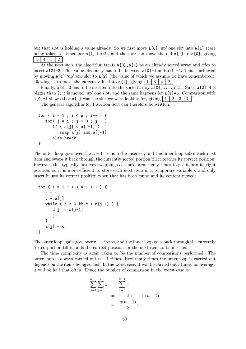
but that slot is holding a value already. So we first move a[0] ‘up’ one slot into a[1] (carebeing taken to remember a[1] first!), and then we can move the old a[1] to a[0], giving1 4 3 2 .

At the next step, the algorithm treats a[0],a[1] as an already sorted array and tries toinsert a[2]=3. This value obviously has to fit between a[0]=1 and a[1]=4. This is achievedby moving a[1] ‘up’ one slot to a[2] (the value of which we assume we have remembered),allowing us to move the current value into a[1], giving 1 3 4 2 .

Finally, a[3]=2 has to be inserted into the sorted array a[0],...,a[2]. Since a[2]=4 isbigger than 2, it is moved ‘up’ one slot, and the same happens for a[1]=3. Comparison witha[0]=1 shows that a[1] was the slot we were looking for, giving 1 2 3 4 .

The general algorithm for Insertion Sort can therefore be written:

for ( i = 1 ; i < n ; i++ ) {

for( j = i ; j > 0 ; j-- )

if ( a[j] < a[j-1] )

swap a[j] and a[j-1]

else break

}

The outer loop goes over the n− 1 items to be inserted, and the inner loop takes each nextitem and swaps it back through the currently sorted portion till it reaches its correct position.However, this typically involves swapping each next item many times to get it into its rightposition, so it is more efficient to store each next item in a temporary variable c and onlyinsert it into its correct position when that has been found and its content moved:

for ( i = 1 ; i < n ; i++ ) {

j = i

c = a[j]

while ( j > 0 && c < a[j-1] ) {

a[j] = a[j-1]

j--

}

a[j] = c

}

The outer loop again goes over n−1 items, and the inner loop goes back through the currentlysorted portion till it finds the correct position for the next item to be inserted.

The time complexity is again taken to be the number of comparisons performed. Theouter loop is always carried out n − 1 times. How many times the inner loop is carried outdepends on the items being sorted. In the worst case, it will be carried out i times; on average,it will be half that often. Hence the number of comparison in the worst case is:

n−1∑

i=1

i∑

j=1

1 =

n−1∑

i=1

i

= 1 + 2 + · · · + (n − 1)

=n(n − 1)

2;

60

and in the average case it is half that, namely n(n − 1)/4. Thus average and worst casenumber of steps for of Insertion Sort are both proportional to n2, and hence the average andworst case time complexities are both O(n2).

8.6 Selection Sort

Selection Sort is (not surprisingly) a form of selection sorting . It first finds the smallest itemand puts it into a[0] by exchanging it with whichever item is in that position already. Thenit finds the second-smallest item and exchanges it with the item in a[1]. It continues thisway until the whole array is sorted. More generally, at the ith stage, Selection Sort finds theith-smallest item and swaps it with the item in a[i-1]. Obviously there is no need to checkfor the ith-smallest item in the first i − 1 elements of the array.

For the example starting array 4 1 3 2 , Selection Sort first finds the smallestitem in the whole array, which is a[1]=1, and swaps this value with that in a[0] giving1 4 3 2 . Then, for the second step, it finds the smallest item in the reduced array

a[1],a[2],a[3], that is a[3]=2, and swaps that into a[1], giving 1 2 3 4 . Finally, itfinds the smallest of the reduced array a[2],a[3], that is a[2]=3, and swaps that into a[2],or recognizes that a swap is not needed, giving 1 2 3 4 .

The general algorithm for Selection Sort can be written:

for ( i = 0 ; i < n-1 ; i++ ) {

k = i

for ( j = i+1 ; j < n ; j++ )

if ( a[j] < a[k] )

k = j

swap a[i] and a[k]

}

The outer loop goes over the first n−1 positions to be filled, and the inner loop goes throughthe currently unsorted portion to find the next smallest item to fill the next position. Notethat, unlike with Bubble Sort and Insertion Sort, there is exactly one swap for each iterationof the outer loop,

The time complexity is again the number of comparisons carried out. The outer loop iscarried out n− 1 times. In the inner loop, which is carried out (n − 1) − i = n − 1 − i times,one comparison occurs. Hence the total number of comparisons is:

n−2∑

i=0

n−1∑

j=i+1

1 =

n−2∑

i=0

(n − 1 − i)

= (n − 1) + · · · + 2 + 1

=n(n − 1)

2.

Therefore the number of comparisons for Selection Sort is proportional to n2, in the worstcase as well as in the average case, and hence the average and worst case time complexitiesare both O(n2).

Note that Bubblesort, Inserion Sort and Selection Sort all involve two nested for loopsover O(n) items, so it is easy to see that their overall complexities will be O(n2) withouthaving to compute the exact number of comparisons.

61

8.7 Comparison of O(n2) sorting algorithms

We have now seen three different array based sorting algorithms, all based on different sortingstrategies, and all with O(n2) time complexity . So one might imagine that it does not makemuch difference which of these algorithms is used. However, in practice, it can actually makea big difference which algorithm is chosen. The following table shows the measured runningtimes of the three algorithms applied to arrays of integers of the size given in the top row:

Algorithm 128 256 512 1024 O1024 R1024 2048

Bubble Sort 54 221 881 3621 1285 5627 14497Insertion Sort 15 69 276 1137 6 2200 4536Selection Sort 12 45 164 634 643 833 2497

Here O1024 denotes an array with 1024 entries which are already sorted, and R1024 is anarray which is sorted in the reverse order, that is, from biggest to smallest. All the otherarrays were filled randomly. Warning: tables of measurements like this are always dependenton the random ordering used, the implementation of the programming language involved, andon the machine it was run on, and so will never be exactly the same.

So where exactly do these differences come from? For a start, Selection Sort alwaysmakes n(n−1)/2 comparisons, but carries out at most n−1 swaps. Each swap requires threeassignments and takes, in fact, more time than a comparison. Bubble Sort, on the other hand,does a lot of swaps. Insertion Sort does particularly well on data which is sorted already –in such a case, it only makes n − 1 comparisons. It is worth bearing this in mind for someapplications, because if only a few entries are out of place, Insertion Sort can be very quick.These comparisons serve to show that complexity considerations can be rather delicate, andrequire good judgement concerning what operations to count. It is often a good idea to runsome experiments to test the theoretical considerations and see whether any simplificationsmade are realistic in practice. For instance, we have assumed here that all comparisons costthe same, but that may not be true for big numbers or strings of characters.

What exactly to count when considering the complexity of a particular algorithm is alwaysa judgement call. You will have to gain experience before you feel comfortable with makingsuch decisions yourself. Furthermore, when you want to improve the performance of analgorithm, you may want to determine the biggest user of computing resources and focus onimproving that. Something else to be aware of when making these calculations is that it isnot a bad idea to keep track of any constant factors, in particular those that go with thedominating sub-term. In the above examples, the factor applied to the dominating sub-term,namely n2, varies. It is 1/2 for the average case of Bubble Sort and Selection Sort, but only1/4 for Insertion Sort. It is certainly useful to know that an algorithm that is linear willperform better than a quadratic one provided the size of the problem is large enough, but ifyou know that your problem has a size of, say, at most 100, then a complexity of (1/10)n2

will be preferable to one of 1000000n. Or if you know that your program is only ever usedon fairly small samples, then using the simplest algorithm you can find might be beneficialoverall – it is easier to program, and there is not a lot of compute time to be saved.

Finally, the above numbers give you some idea why for program designers, the generalrule is to never use Bubble Sort. It is easy to program, but that is about all it has going forit. You are better off avoiding it altogether.

62

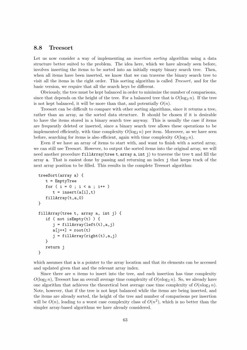
8.8 Treesort

Let us now consider a way of implementing an insertion sorting algorithm using a datastructure better suited to the problem. The idea here, which we have already seen before,involves inserting the items to be sorted into an initially empty binary search tree. Then,when all items have been inserted, we know that we can traverse the binary search tree tovisit all the items in the right order. This sorting algorithm is called Treesort , and for thebasic version, we require that all the search keys be different.

Obviously, the tree must be kept balanced in order to minimize the number of comparisons,since that depends on the height of the tree. For a balanced tree that is O(log2 n). If the treeis not kept balanced, it will be more than that, and potentially O(n).

Treesort can be difficult to compare with other sorting algorithms, since it returns a tree,rather than an array, as the sorted data structure. It should be chosen if it is desirableto have the items stored in a binary search tree anyway. This is usually the case if itemsare frequently deleted or inserted, since a binary search tree allows these operations to beimplemented efficiently, with time complexity O(log2 n) per item. Moreover, as we have seenbefore, searching for items is also efficient, again with time complexity O(log2 n).

Even if we have an array of items to start with, and want to finish with a sorted array,we can still use Treesort. However, to output the sorted items into the original array, we willneed another procedure fillArray(tree t, array a, int j) to traverse the tree t and fill thearray a. That is easiest done by passing and returning an index j that keeps track of thenext array position to be filled. This results in the complete Treesort algorithm:

treeSort(array a) {

t = EmptyTree

for ( i = 0 ; i < n ; i++ )

t = insert(a[i],t)

fillArray(t,a,0)

}

fillArray(tree t, array a, int j) {

if ( not isEmpty(t) ) {

j = fillArray(left(t),a,j)

a[j++] = root(t)

j = fillArray(right(t),a,j)

}

return j

}

which assumes that a is a pointer to the array location and that its elements can be accessedand updated given that and the relevant array index.

Since there are n items to insert into the tree, and each insertion has time complexityO(log2 n), Treesort has an overall average time complexity of O(nlog2 n). So, we already haveone algorithm that achieves the theoretical best average case time complexity of O(nlog2 n).Note, however, that if the tree is not kept balanced while the items are being inserted, andthe items are already sorted, the height of the tree and number of comparisons per insertionwill be O(n), leading to a worst case complexity class of O(n2), which is no better than thesimpler array-based algorithms we have already considered.

63

8.9 Heapsort

We now consider another way of implementing a selection sorting algorithm using a moreefficient data structure we have already studied. The underlying idea here is that it wouldhelp if we could pre-arrange the data so that selecting the smallest/biggest entry becomeseasier. For that, remember the idea of a priority queue discussed earlier. We can take thevalue of an item to be its priority. Then, if we remove the item with the highest priority ateach step we can fill an array in order ‘from the rear’, starting with the biggest item.

Priority queues can be implemented in a number of different ways, and we have alreadystudied a straightforward implementation using binary heap trees in Chapter 7. However,there may be a better way, so it is worth considering the other possibilities.

An obvious way of implementing them would be using a sorted array, so that the entrywith the highest priority appears in a[n]. Removing this item would be very simple, butinserting a new item would always involve finding the right position and shifting a number ofitems to the right to make room for it. For example, inserting a 3 into the queue [1, 2, 4]:

n 0 1 2 3 4 5

a[n] 1 2 4

n 0 1 2 3 4 5

a[n] 1 2 4

n 0 1 2 3 4 5

a[n] 1 2 3 4

That kind of item insertion is effectively insertion sort and clearly inefficient in general, ofO(n) complexity rather than O(log2 n) with a binary heap tree.

Another approach would be to use an unsorted array. In this case, a new item would beinserted by just putting it into a[n+1], but to delete the entry with the highest priority wouldinvolve having to find it first. Then, after that, the last item would have to be swapped intothe gap, or all items with a higher index ‘shifted down’. Again, that kind of item deletion isclearly inefficient in general, of O(n) complexity rather than O(log2 n) with a heap tree.

Thus, of those three representations, only one is of use in carrying out the above ideaefficiently. An unsorted array is what we started from, so that is not any help, and orderingthe array is what we are trying to achieve, so heaps are the way forward.

To make use of binary heap trees, we first have to take the unsorted array and re-arrangeit so that it satisies the heap tree priority ordering. We have already studied the heapifyalgorithm which can do that with O(n) time complexity. Then we need to extract the sortedarray from it. In the heap tree, the item with the highest priority, that is the largest item, isalways in a[1]. In the sorted array, it should be in the last position a[n]. If we simply swapthe two, we will have that item at the right position of the array, and also have begun thestandard procedure of removing the root of the heap-tree, since a[n] is precisely the item thatwould be moved into the root position at the next step. Since a[n] now contains the correctitem, we will never have to look at it again. Instead, we just take the items a[1],...,a[n-1]and bring them back into a heap-tree form using the bubble down procedure on the new root,which we know to have complexity O(log2 n).

Now the second largest item is in position a[1], and its final position should be a[n-1],so we now swap these two items. Then we rearrange a[1],...,a[n-2] back into a heap treeusing the bubble down procedure on the new root. And so on.

64

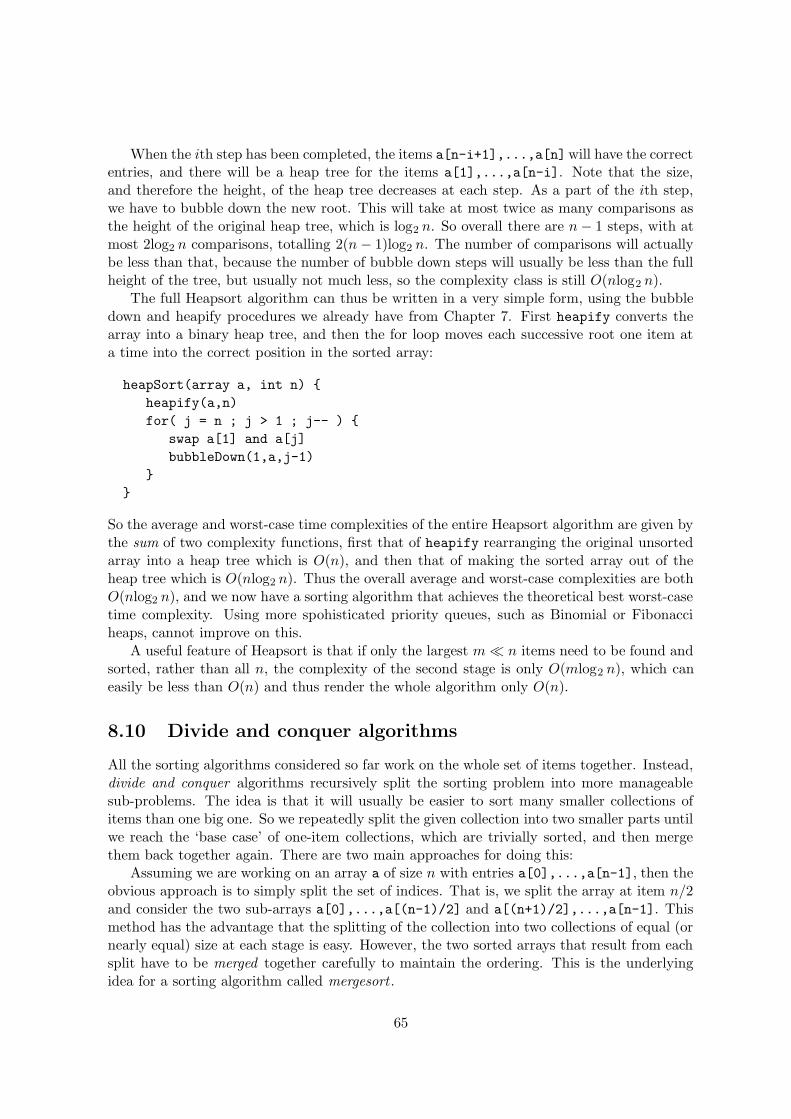
When the ith step has been completed, the items a[n-i+1],...,a[n]will have the correctentries, and there will be a heap tree for the items a[1],...,a[n-i]. Note that the size,and therefore the height, of the heap tree decreases at each step. As a part of the ith step,we have to bubble down the new root. This will take at most twice as many comparisons asthe height of the original heap tree, which is log2 n. So overall there are n − 1 steps, with atmost 2log2 n comparisons, totalling 2(n − 1)log2 n. The number of comparisons will actuallybe less than that, because the number of bubble down steps will usually be less than the fullheight of the tree, but usually not much less, so the complexity class is still O(nlog2 n).

The full Heapsort algorithm can thus be written in a very simple form, using the bubbledown and heapify procedures we already have from Chapter 7. First heapify converts thearray into a binary heap tree, and then the for loop moves each successive root one item ata time into the correct position in the sorted array:

heapSort(array a, int n) {

heapify(a,n)

for( j = n ; j > 1 ; j-- ) {

swap a[1] and a[j]

bubbleDown(1,a,j-1)

}

}

So the average and worst-case time complexities of the entire Heapsort algorithm are given bythe sum of two complexity functions, first that of heapify rearranging the original unsortedarray into a heap tree which is O(n), and then that of making the sorted array out of theheap tree which is O(nlog2 n). Thus the overall average and worst-case complexities are bothO(nlog2 n), and we now have a sorting algorithm that achieves the theoretical best worst-casetime complexity. Using more spohisticated priority queues, such as Binomial or Fibonacciheaps, cannot improve on this.

A useful feature of Heapsort is that if only the largest m � n items need to be found andsorted, rather than all n, the complexity of the second stage is only O(mlog2 n), which caneasily be less than O(n) and thus render the whole algorithm only O(n).

8.10 Divide and conquer algorithms

All the sorting algorithms considered so far work on the whole set of items together. Instead,divide and conquer algorithms recursively split the sorting problem into more manageablesub-problems. The idea is that it will usually be easier to sort many smaller collections ofitems than one big one. So we repeatedly split the given collection into two smaller parts untilwe reach the ‘base case’ of one-item collections, which are trivially sorted, and then mergethem back together again. There are two main approaches for doing this:

Assuming we are working on an array a of size n with entries a[0],...,a[n-1], then theobvious approach is to simply split the set of indices. That is, we split the array at item n/2and consider the two sub-arrays a[0],...,a[(n-1)/2] and a[(n+1)/2],...,a[n-1]. Thismethod has the advantage that the splitting of the collection into two collections of equal (ornearly equal) size at each stage is easy. However, the two sorted arrays that result from eachsplit have to be merged together carefully to maintain the ordering. This is the underlyingidea for a sorting algorithm called mergesort .

65

Another approach would be to split the array in such a way that, at each stage, allthe items in the first collection are no bigger than all the items in the second collection. Thesplitting here is obviously more complex, but all we have to do to put the pieces back togetheragain at each stage is to take the first sorted array followed by the second sorted array. Thisis the underlying idea for a sorting algorithm called Quicksort .

We shall now look in detail at how these two approaches work in practice.

8.11 Quicksort

The general idea here is to repeatedly split (or partition) the given array in such a way thatall the items in the first sub-array are smaller than all the items in the second sub-array, andthen concatenate all the sub-arrays to give the sorted full array.

How to partition. The important question is how to perform this kind of splitting mostefficiently. If the array is very simple, for example [4,3,7,8,1,6], then a good split would be toput all the items smaller than 5 into one part, giving [4,3,1], and all the items bigger thanor equal to 5 into the other, that is [7,8,6]. Indeed, moving all items with a smaller key thansome given value into one sub-array, and all entries with a bigger or equal key into the othersub-array is the standard Quicksort strategy. The value that defines the split is called thepivot . However, it is not obvious what is the best way to choose the pivot value.

One situation that we absolutely have to avoid is splitting the array into an empty sub-array and the whole array again. If we do this, the algorithm will not just perform badly, itwill not even terminate. However, if the pivot is chosen to be an item in the array, and thepivot is kept in between and separate from both sub-arrays, then the sub-arrays being sortedat each recursion will always be at least one item shorter than the previous array, and thealgorithm is guaranteed to terminate.

Thus, it proves convenient to split the array at each stage into the sub-array of valuessmaller than or equal to some chosen pivot item, followed by that chosen pivot item, followedby the sub-array of values greater than or equal to the chosen pivot item. Moreover, to savespace, we do not actually split the array into smaller arrays. Instead, we simply rearrange thewhole array to reflect the splitting. We say that we partition the array, and the Quicksortalgorithm is then applied to the sub-arrays of this partitioned array.

In order for the algorithm to be called recursively, to sort ever smaller parts of the originalarray, we need to tell it which part of the array is currently under consideration. Therefore,Quicksort is called giving the lowest index (left) and highest index (right) of the sub-arrayit must work on. Thus the algorithm takes the form:

quicksort(array a, int left, int right) {

if ( left < right ) {

pivotindex = partition(a,left,right)

quicksort(a,left,pivotindex-1)

quicksort(a,pivotindex+1,right)

}

}

for which the initial call would be quicksort(a,0,n-1) and the array a at the end is sorted.The crucial part of this is clearly the partition(a, left, right) procedure that rearranges

66

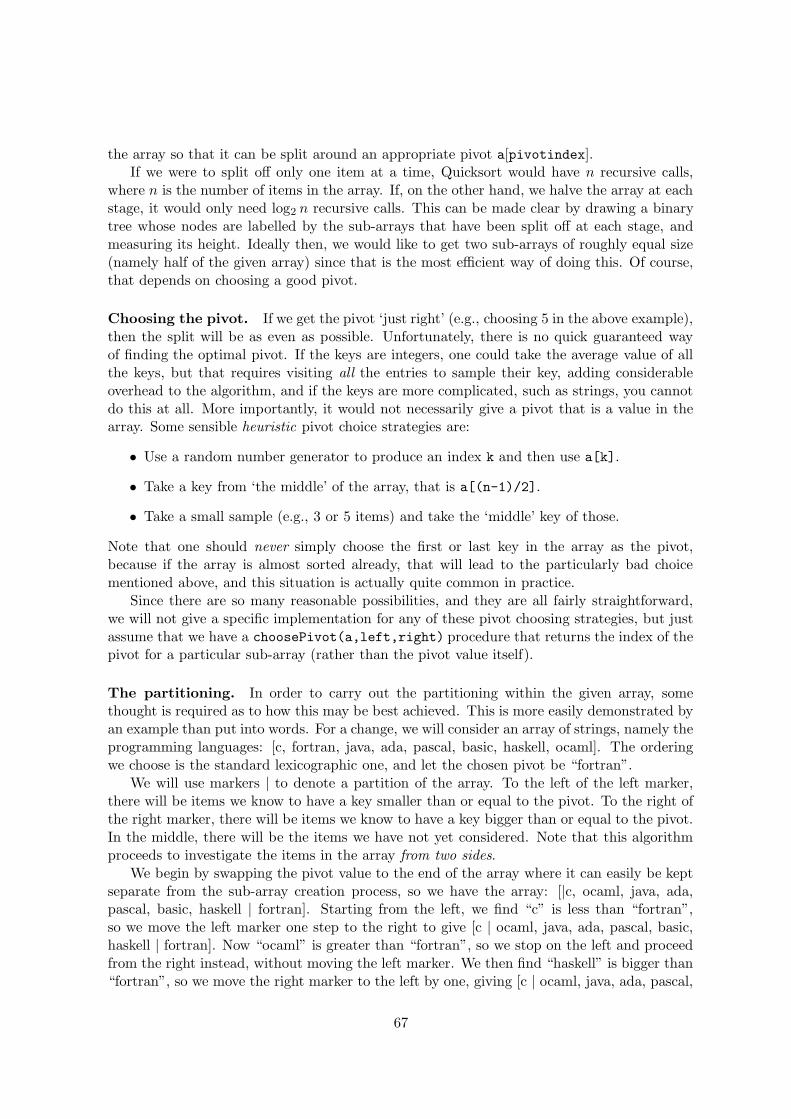
the array so that it can be split around an appropriate pivot a[pivotindex].If we were to split off only one item at a time, Quicksort would have n recursive calls,

where n is the number of items in the array. If, on the other hand, we halve the array at eachstage, it would only need log2 n recursive calls. This can be made clear by drawing a binarytree whose nodes are labelled by the sub-arrays that have been split off at each stage, andmeasuring its height. Ideally then, we would like to get two sub-arrays of roughly equal size(namely half of the given array) since that is the most efficient way of doing this. Of course,that depends on choosing a good pivot.

Choosing the pivot. If we get the pivot ‘just right’ (e.g., choosing 5 in the above example),then the split will be as even as possible. Unfortunately, there is no quick guaranteed wayof finding the optimal pivot. If the keys are integers, one could take the average value of allthe keys, but that requires visiting all the entries to sample their key, adding considerableoverhead to the algorithm, and if the keys are more complicated, such as strings, you cannotdo this at all. More importantly, it would not necessarily give a pivot that is a value in thearray. Some sensible heuristic pivot choice strategies are:

• Use a random number generator to produce an index k and then use a[k].

• Take a key from ‘the middle’ of the array, that is a[(n-1)/2].

• Take a small sample (e.g., 3 or 5 items) and take the ‘middle’ key of those.

Note that one should never simply choose the first or last key in the array as the pivot,because if the array is almost sorted already, that will lead to the particularly bad choicementioned above, and this situation is actually quite common in practice.

Since there are so many reasonable possibilities, and they are all fairly straightforward,we will not give a specific implementation for any of these pivot choosing strategies, but justassume that we have a choosePivot(a,left,right) procedure that returns the index of thepivot for a particular sub-array (rather than the pivot value itself).

The partitioning. In order to carry out the partitioning within the given array, somethought is required as to how this may be best achieved. This is more easily demonstrated byan example than put into words. For a change, we will consider an array of strings, namely theprogramming languages: [c, fortran, java, ada, pascal, basic, haskell, ocaml]. The orderingwe choose is the standard lexicographic one, and let the chosen pivot be “fortran”.

We will use markers | to denote a partition of the array. To the left of the left marker,there will be items we know to have a key smaller than or equal to the pivot. To the right ofthe right marker, there will be items we know to have a key bigger than or equal to the pivot.In the middle, there will be the items we have not yet considered. Note that this algorithmproceeds to investigate the items in the array from two sides.

We begin by swapping the pivot value to the end of the array where it can easily be keptseparate from the sub-array creation process, so we have the array: [|c, ocaml, java, ada,pascal, basic, haskell | fortran]. Starting from the left, we find “c” is less than “fortran”,so we move the left marker one step to the right to give [c | ocaml, java, ada, pascal, basic,haskell | fortran]. Now “ocaml” is greater than “fortran”, so we stop on the left and proceedfrom the right instead, without moving the left marker. We then find “haskell” is bigger than“fortran”, so we move the right marker to the left by one, giving [c | ocaml, java, ada, pascal,

67

basic, | haskell, fortran]. Now “basic” is smaller than “fortran”, so we have two keys, “ocaml”and “basic”, which are ‘on the wrong side’. We therefore swap them, which allows us to moveboth the left and the right marker one step further towards the middle. This brings us to [c,basic | java, ada, pascal | ocaml, haskell, fortran]. Now we proceed from the left once again,but “java” is bigger than “fortran”, so we stop there and switch to the right. Then “pascal”is bigger than “fortran”, so we move the right marker again. We then find “ada”, which issmaller than the pivot, so we stop. We have now got [c, basic | java, ada, | pascal, ocaml,haskell, fortran]. As before, we want to swap “java” and “ada”, which leaves the left and theright markers in the same place: [c, basic, ada, java | | pascal, ocaml, haskell, fortran], so westop. Finally, we swap the pivot back from the last position into the position immediatelyafter the markers to give [c, basic, ada, java | | fortran, ocaml, haskell, pascal].

Since we obviously cannot have the marker indices ‘between’ array entries, we will as-sume the left marker is on the left of a[leftmark] and the right marker is to the rightof a[rightmark]. The markers are therefore ‘in the same place’ once rightmark becomessmaller than leftmark, which is when we stop. If we assume that the keys are integers, wecan write the partitioning procedure, that needs to return the final pivot position, as:

partition(array a, int left, int right) {

pivotindex = choosePivot(a, left, right)

pivot = a[pivotindex]

swap a[pivotindex] and a[right]

leftmark = left

rightmark = right - 1

while (leftmark <= rightmark) {

while (leftmark <= rightmark and a[leftmark] <= pivot)

leftmark++

while (leftmark <= rightmark and a[rightmark] >= pivot)

rightmark--

if (leftmark < rightmark)

swap a[leftmark++] and a[rightmark--]

}

swap a[leftmark] and a[right]

return leftmark

}

This achieves a partitioning that ends with the same items in the array, but in a differentorder, with all items to the left of the returned pivot position smaller or equal to the pivotvalue, and all items to the right greater or equal to the pivot value.

Note that this algorithm doesn’t require any extra memory – it just swaps the items inthe original array. A conceptually simpler approach, that requires more memory and copying,would be to simply go systematically through the whole array, re-filling the array a with itemsless than or equal to the pivot, and filling a second array b with items greater or equal to thepivot, and finally copying the array b into the end of a:

partition2(array a, int left, int right) {

create new array b of size right-left+1

pivotindex = choosePivot(a, left, right)

68

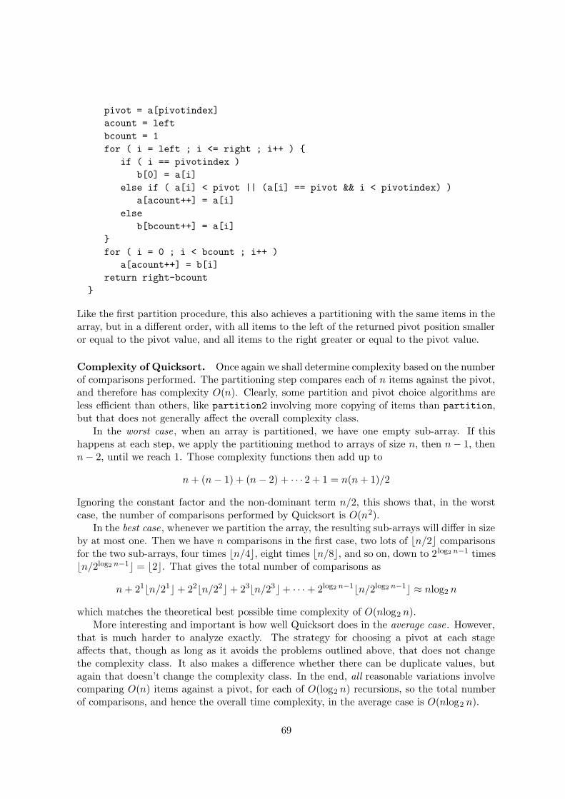
pivot = a[pivotindex]

acount = left

bcount = 1

for ( i = left ; i <= right ; i++ ) {

if ( i == pivotindex )

b[0] = a[i]

else if ( a[i] < pivot || (a[i] == pivot && i < pivotindex) )

a[acount++] = a[i]

else

b[bcount++] = a[i]

}

for ( i = 0 ; i < bcount ; i++ )

a[acount++] = b[i]

return right-bcount

}

Like the first partition procedure, this also achieves a partitioning with the same items in thearray, but in a different order, with all items to the left of the returned pivot position smalleror equal to the pivot value, and all items to the right greater or equal to the pivot value.

Complexity of Quicksort. Once again we shall determine complexity based on the numberof comparisons performed. The partitioning step compares each of n items against the pivot,and therefore has complexity O(n). Clearly, some partition and pivot choice algorithms areless efficient than others, like partition2 involving more copying of items than partition,but that does not generally affect the overall complexity class.

In the worst case, when an array is partitioned, we have one empty sub-array. If thishappens at each step, we apply the partitioning method to arrays of size n, then n − 1, thenn − 2, until we reach 1. Those complexity functions then add up to

n + (n − 1) + (n − 2) + · · · 2 + 1 = n(n + 1)/2

Ignoring the constant factor and the non-dominant term n/2, this shows that, in the worstcase, the number of comparisons performed by Quicksort is O(n2).

In the best case, whenever we partition the array, the resulting sub-arrays will differ in sizeby at most one. Then we have n comparisons in the first case, two lots of bn/2c comparisonsfor the two sub-arrays, four times bn/4c, eight times bn/8c, and so on, down to 2 log2 n−1 timesbn/2log2 n−1c = b2c. That gives the total number of comparisons as

n + 21bn/21c + 22bn/22c + 23bn/23c + · · · + 2log2 n−1bn/2log2 n−1c ≈ nlog2 n

which matches the theoretical best possible time complexity of O(nlog2 n).More interesting and important is how well Quicksort does in the average case. However,

that is much harder to analyze exactly. The strategy for choosing a pivot at each stageaffects that, though as long as it avoids the problems outlined above, that does not changethe complexity class. It also makes a difference whether there can be duplicate values, butagain that doesn’t change the complexity class. In the end, all reasonable variations involvecomparing O(n) items against a pivot, for each of O(log2 n) recursions, so the total numberof comparisons, and hence the overall time complexity, in the average case is O(nlog2 n).

69

Like Heapsort, when only the largest m � n items need to be found and sorted, ratherthan all n, Quicksort can be modified to result in reduced time complexity. In this case, onlythe first sub-array needs to be processed at each stage, until the sub-array sizes exceed m. Inthat situation, for the best case, the total number of comparisons is reduced to

n + 1bn/21c + 1bn/22c + 1bn/23c + · · · + mlog2 m ≈ 2n.

rendering the time complexity of the whole modified algorithm only O(n). For the averagecase, the computation is again more difficult, but as long as the key problems outlined aboveare avoided, the average-case complexity of this special case is also O(n).

Improving Quicksort. It is always worthwhile spending some time optimizing the strategyfor defining the pivot, since the particular problem in question might well allow for a morerefined approach. Generally, the pivot will be better if more items are sampled before itis being chosen. For example, one could check several randomly chosen items and take the‘middle’ one of those, the so called median. Note that in order to find the median of all theitems, we would end up having to make n2 comparisons, so we cannot do that without makingQuicksort unattractively slow.

Quicksort is rarely the most suitable algorithm if the problem size is small. The reason forthis is all the overheads from the recursion (e.g., storing all the return addresses and formalparameters). Hence once the sub-problem become ‘small’ (a size of 16 is often suggested inthe literature), Quicksort should stop calling itself and instead sort the remaining sub-arraysusing a simpler algorithm such as Selection Sort.

8.12 Mergesort

The other divide and conquer sorting strategy based on repeatedly splitting the array ofitems into two sub-arrays, mentioned in Section 8.10, is called mergesort . This simply splitsthe array at each stage into its first and last half, without any reordering of the items in it.However, that will obviously not result in a set of sorted sub-arrays that we can just appendto each other at the end. So mergesort needs another procedure merge that merges two sortedsub-arrays into another sorted array. As with binary search in Section 3.4, integer variablesleft and right can be used to refer to the lower and upper index of the relevant array, andmid refers to the end of its left sub-array. Thus a suitable mergesort algorithm is:

mergesort(array a, int left, int right) {

if ( left < right ) {

mid = (left + right) / 2

mergesort(a, left, mid)

mergesort(a, mid+1, right)

merge(a, left, mid, right)

}

}

Note that it would be relatively simple to modify this mergesort algorithm to operate onlinked lists (of known length) rather than arrays. To ‘split’ such a list into two, all one has todo is set the pointer of the bn/2cth list entry to null, and use the previously-pointed-to nextentry as the head of the new second list. Of course, care needs to be taken to keep the listsize information intact, and effort is required to find the crucial pointer for each split.

70

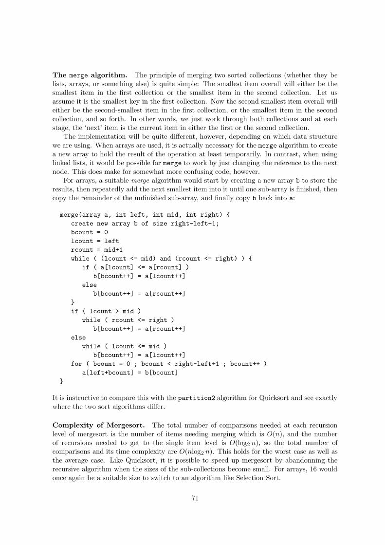
The merge algorithm. The principle of merging two sorted collections (whether they belists, arrays, or something else) is quite simple: The smallest item overall will either be thesmallest item in the first collection or the smallest item in the second collection. Let usassume it is the smallest key in the first collection. Now the second smallest item overall willeither be the second-smallest item in the first collection, or the smallest item in the secondcollection, and so forth. In other words, we just work through both collections and at eachstage, the ‘next’ item is the current item in either the first or the second collection.

The implementation will be quite different, however, depending on which data structurewe are using. When arrays are used, it is actually necessary for the merge algorithm to createa new array to hold the result of the operation at least temporarily. In contrast, when usinglinked lists, it would be possible for merge to work by just changing the reference to the nextnode. This does make for somewhat more confusing code, however.

For arrays, a suitable merge algorithm would start by creating a new array b to store theresults, then repeatedly add the next smallest item into it until one sub-array is finished, thencopy the remainder of the unfinished sub-array, and finally copy b back into a:

merge(array a, int left, int mid, int right) {

create new array b of size right-left+1;

bcount = 0

lcount = left

rcount = mid+1

while ( (lcount <= mid) and (rcount <= right) ) {

if ( a[lcount] <= a[rcount] )

b[bcount++] = a[lcount++]

else

b[bcount++] = a[rcount++]

}

if ( lcount > mid )

while ( rcount <= right )

b[bcount++] = a[rcount++]

else

while ( lcount <= mid )

b[bcount++] = a[lcount++]

for ( bcount = 0 ; bcount < right-left+1 ; bcount++ )

a[left+bcount] = b[bcount]

}

It is instructive to compare this with the partition2 algorithm for Quicksort and see exactlywhere the two sort algorithms differ.

Complexity of Mergesort. The total number of comparisons needed at each recursionlevel of mergesort is the number of items needing merging which is O(n), and the numberof recursions needed to get to the single item level is O(log2 n), so the total number ofcomparisons and its time complexity are O(nlog2 n). This holds for the worst case as well asthe average case. Like Quicksort, it is possible to speed up mergesort by abandonning therecursive algorithm when the sizes of the sub-collections become small. For arrays, 16 wouldonce again be a suitable size to switch to an algorithm like Selection Sort.

71

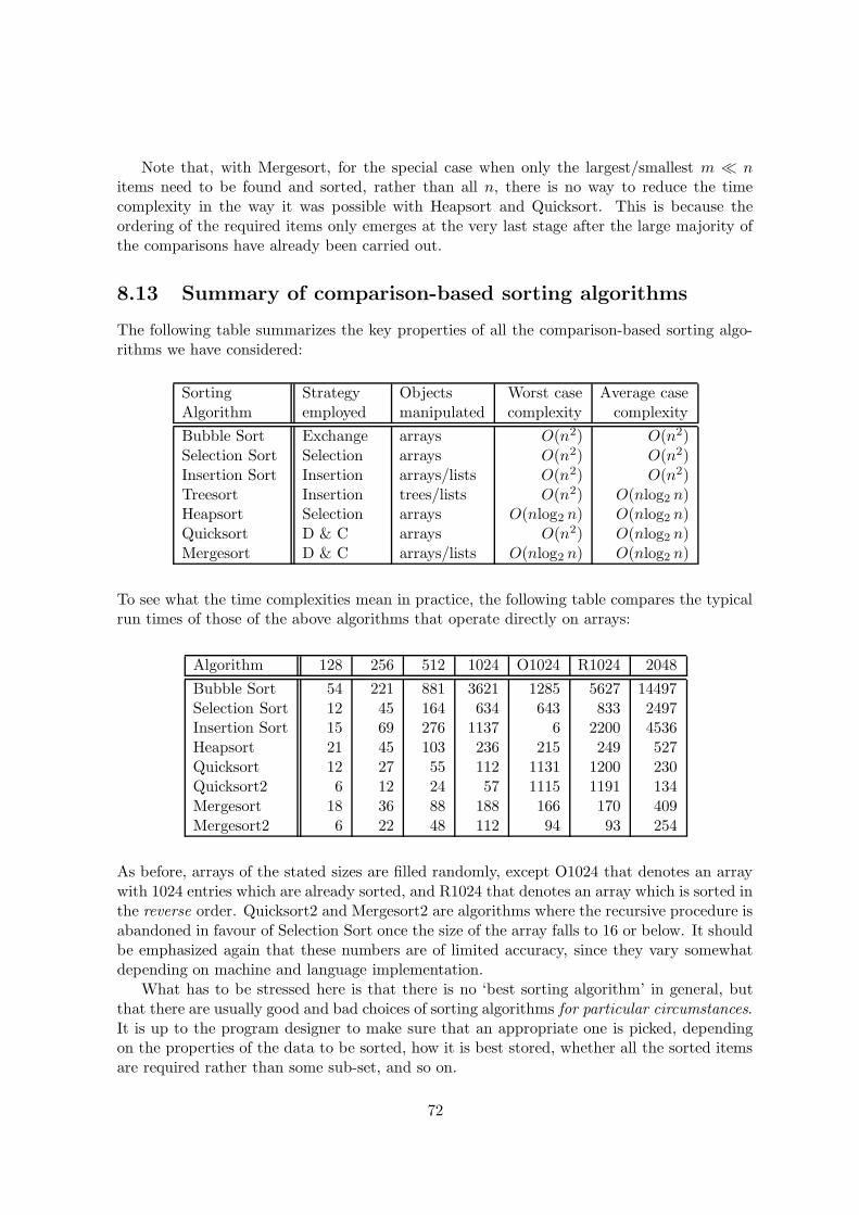
Note that, with Mergesort, for the special case when only the largest/smallest m � nitems need to be found and sorted, rather than all n, there is no way to reduce the timecomplexity in the way it was possible with Heapsort and Quicksort. This is because theordering of the required items only emerges at the very last stage after the large majority ofthe comparisons have already been carried out.

8.13 Summary of comparison-based sorting algorithms

The following table summarizes the key properties of all the comparison-based sorting algo-rithms we have considered:

Sorting Strategy Objects Worst case Average caseAlgorithm employed manipulated complexity complexity

Bubble Sort Exchange arrays O(n2) O(n2)Selection Sort Selection arrays O(n2) O(n2)Insertion Sort Insertion arrays/lists O(n2) O(n2)Treesort Insertion trees/lists O(n2) O(nlog2 n)Heapsort Selection arrays O(nlog2 n) O(nlog2 n)Quicksort D & C arrays O(n2) O(nlog2 n)Mergesort D & C arrays/lists O(nlog2 n) O(nlog2 n)

To see what the time complexities mean in practice, the following table compares the typicalrun times of those of the above algorithms that operate directly on arrays:

Algorithm 128 256 512 1024 O1024 R1024 2048

Bubble Sort 54 221 881 3621 1285 5627 14497Selection Sort 12 45 164 634 643 833 2497Insertion Sort 15 69 276 1137 6 2200 4536Heapsort 21 45 103 236 215 249 527Quicksort 12 27 55 112 1131 1200 230Quicksort2 6 12 24 57 1115 1191 134Mergesort 18 36 88 188 166 170 409Mergesort2 6 22 48 112 94 93 254

As before, arrays of the stated sizes are filled randomly, except O1024 that denotes an arraywith 1024 entries which are already sorted, and R1024 that denotes an array which is sorted inthe reverse order. Quicksort2 and Mergesort2 are algorithms where the recursive procedure isabandoned in favour of Selection Sort once the size of the array falls to 16 or below. It shouldbe emphasized again that these numbers are of limited accuracy, since they vary somewhatdepending on machine and language implementation.

What has to be stressed here is that there is no ‘best sorting algorithm’ in general, butthat there are usually good and bad choices of sorting algorithms for particular circumstances.It is up to the program designer to make sure that an appropriate one is picked, dependingon the properties of the data to be sorted, how it is best stored, whether all the sorted itemsare required rather than some sub-set, and so on.

72

8.14 Non-comparison-based sorts

All the above sorting algorithms have been based on comparisons of the items to be sorted,and we have seen that we can’t get time complexity better than O(nlog2 n) with comparisonbased algorithms. However, in some circumstances it is possible to do better than that withsorting algorithms that are not based on comparisons.

It is always worth thinking about the data that needs to be sorted, and whether com-parisons really are required. For example, suppose you know the items to be sorted are thenumbers from 0 to n − 1. How would you sort those? The answer is surprisingly simple. Weknow that we have n entries in the array and we know exactly which items should go thereand in which order. This is a very unusual situation as far as general sorting is concerned, yetthis kind of thing often comes up in every-day life. For example, when a hotel needs to sortthe room keys for its 100 rooms. Rather than employing one of the comparison-based sortingalgorithms, in this situation we can do something much simpler. We can simply put the itemsdirectly in the appropriate places, using an algorithm such as that as shown in Figure 8.1:

0

0 1 3

243 1

2 4

create array b of size n

for ( i = 0 ; i < n ; i++ )

b[a[i]] = a[i]

copy array b into array a

Figure 8.1: Simply put the items in the right order using their values.

This algorithm uses a second array b to hold the results, which is clearly not very memoryefficient, but it is possible to do without that. One can use a series of swaps within array a

to get the items in the right positions as shown in Figure 8.2:

3 0 1 24

01 3 24

310 24

310 2 4

i=0

i=1

i=0

i=2

for ( i = 0 ; i < n; i++ ) {

while ( a[i] != i )

swap a[a[i]] and a[i]

}

Figure 8.2: Swapping the items into the right order without using a new array.

As far as time complexity is concerned, it is obviously not appropriate here to count thenumber of comparisons. Instead, it is the number of swaps or copies that is important. Thealgorithm of Figure 8.1 performs n copies to fill array b and then another n to return the resultto array a, so the overall time complexity is O(n). The time complexity of the algorithm of

73

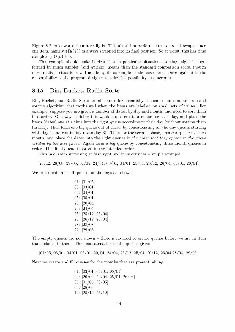
Figure 8.2 looks worse than it really is. This algorithm performs at most n − 1 swaps, sinceone item, namely a[a[i]] is always swapped into its final position. So at worst, this has timecomplexity O(n) too.

This example should make it clear that in particular situations, sorting might be per-formed by much simpler (and quicker) means than the standard comparison sorts, thoughmost realistic situations will not be quite as simple as the case here. Once again it is theresponsibility of the program designer to take this possibility into account.

8.15 Bin, Bucket, Radix Sorts

Bin, Bucket, and Radix Sorts are all names for essentially the same non-comparison-basedsorting algorithm that works well when the items are labelled by small sets of values. Forexample, suppose you are given a number of dates, by day and month, and need to sort theminto order. One way of doing this would be to create a queue for each day, and place theitems (dates) one at a time into the right queue according to their day (without sorting themfurther). Then form one big queue out of these, by concatenating all the day queues startingwith day 1 and continuing up to day 31. Then for the second phase, create a queue for eachmonth, and place the dates into the right queues in the order that they appear in the queuecreated by the first phase. Again form a big queue by concatenating these month queues inorder. This final queue is sorted in the intended order.

This may seem surprising at first sight, so let us consider a simple example:

[25/12, 28/08, 29/05, 01/05, 24/04, 03/01, 04/01, 25/04, 26/12, 26/04, 05/01, 20/04].

We first create and fill queues for the days as follows:

01: [01/05]03: [03/01]04: [04/01]05: [05/01]20: [20/04]24: [24/04]25: [25/12, 25/04]26: [26/12, 26/04]28: [28/08]29: [29/05]

The empty queues are not shown – there is no need to create queues before we hit an itemthat belongs to them. Then concatenation of the queues gives:

[01/05, 03/01, 04/01, 05/01, 20/04, 24/04, 25/12, 25/04, 26/12, 26/04,28/08, 29/05].

Next we create and fill queues for the months that are present, giving:

01: [03/01, 04/01, 05/01]04: [20/04, 24/04, 25/04, 26/04]05: [01/05, 29/05]08: [28/08]12: [25/12, 26/12]

74

Finally, concatenating all these queues gives the items in the required order:

[03/01, 04/01, 05/01, 20/04, 24/04, 25/04, 26/04, 01/05, 29/05, 28/08, 25/12, 26/12].

This is called Two-phase Radix Sorting , since there are clearly two phases to it.If you know that your items are all (at most) two-digit integers, you can use Radix Sort

to sort them, by creating queues for the last digit first and then doing the same for the firstone. Similarly, if you know that your keys are all strings consisting of three characters, youcan apply Radix Sort. You would first sort according to the third character, then the second,and finally the first (giving a Three phase Radix Sort).

The extension of this idea to give a general sorting algorithm should be obvious. Thecrucial aspect is that you always perform the queuing in the order of the significance of eachcriteria, with the least significant criterion in the first phase.

Note that at no point, does the the algorithm actually compare any items at all. Thiskind of algorithm makes use of the fact that the items are from a strictly restricted set, or,in other words, of a particular form which is known a priori. The complexity class of thisalgorithm is O(n), since at every phase, each item is looked at precisely once. The creationof queues does cause some overhead, of course, but this is not worse than linear.

75

Chapter 9

Hash Tables

We have already seen a number of different ways of storing items in a computer: arrays andvariants thereof (e.g., sorted and unsorted arrays, heap trees), linked lists, and trees (e.g.,binary search trees, heap trees). We have also seen that these approaches can perform quitedifferently when it comes to the particular tasks we expect to carry out, and that the bestway of storing data does not exist in general, but differs from situation to situation.

This chapter looks at another way of storing data, that is quite different from the ones wehave seen so far. It has impressive performance as far as time is concerned, but that advantageis payed for by needing more space (i.e., memory), as well as by being quite sophisticated andtherefore not entirely straightforward to describe or implement.

We first need to specify what we expect to be able to do with this way of storing data,without considering how it is actually implemented. In other words, we need to outline anabstract data type. This is similar to what you will generally do when first trying to implementa class in Java: You should think about the operations you wish to perform on the objectsof that class. You may also want to specify a few variables that you know will definitely beneeded for that class, but this does not usually come into defining an abstract data type.The approach we have been following for defining abstract data types in this module is bydescribing the crucial operations in plain English, trusting that they are simple enough to notneed further explanations. In general, what is needed is a specification for the abstract datatype in question. An important aspect of studying software engineering is to learn about anduse more formal approaches to this way of operating.

After we have decided what our specification is, we then need to choose a data structurein order to implement the abstract data type. The data structure to be considered in thischapter is known as a hash table.

9.1 The Table abstract data type

The specification of the table abstract data type is as follows:

1. A table can be used to store objects, for example

012 Johnny English Spy

007 James Bond Spy

583 Alex Rider Spy

721 Sherlock Holmes Detective

722 James Moriarty Villain

76

2. The objects can be arbitrarily complicated. However, for our purposes, the only relevantdetail is that each object has a unique key , and that their keys can be compared forequality. The keys are used in order to identify objects in much the way we have donefor searching and sorting.

3. We assume that there are methods or procedures for:

(a) determining whether the table is empty or full;

(b) inserting a new object into the table, provided the table is not already full;

(c) given a key, retrieving the object with that key;

(d) given a key, updating the item with that key (usually by replacing the item with anew one with the same key, which is what we will assume here, or by overwritingsome of the items variables);

(e) given a key, deleting the object with that key, provided that object is stored in thetable;

(f) listing all the items in the table (if there is an order on the keys then we wouldexpect this to occur in increasing order).

Notice that we are assuming that each object is uniquely identified by its key.In a programming language such as Java, we could write an interface for this abstract

data type as follows, where we assume here that keys are objects of a class we call Key andwe have records of a class called Record:

interface Table {

Boolean isEmpty();

Boolean isFull();

void Insert(Record);

Record Retrieve(Key);

void Update(Record);

void Delete{Key};

void Traverse();

}

Note that we have not fixed how exactly the storage of records should work – that is some-thing that comes with the implementation. Also note that you could give an interface tosomebody else, who could then write a program which performs operations on tables withoutever knowing how they are implemented. You could certainly carry out all those operationswith binary search trees and sorted or unsorted arrays if you wished. The former even hasthe advantage that a binary search tree never becomes full as such, it is only limited by thesize of the memory.

This general approach follows the sensible and commonly used way to go about defining aJava class: First think about what it is you want to do with the class, and only then wonderabout how exactly you might implement the methods. Thus, languages such as Java supportmechanisms for defining abstract data types. But notice that, as opposed to a specificationin plain English, such as the above, a definition of an interface is only a partial specificationof an abstract data type, because it does not explain what the methods are supposed to do;it only explains how they are called.

77

9.2 Implementations of the table data structure

There are three key approaches for implementing the table data structure. The first two wehave studied already, and the third is the topic of this chapter:

Implementation via sorted arrays. Let us assume that we want to implement the tabledata structure using a sorted array . Whether it is full or empty can easily be determined inconstant time if we have a variable for the size. Then to insert an element we first have to findits proper position, which will take on average the same time as finding an element. To find anelement (which is necessary for all other operations apart from traversal), we can use binarysearch as described in in Section 3.4, so this takes O(log2 n). This is also the complexity forretrieval and update. However, if we wish to delete or insert an item, we will have to shiftwhat is ‘to the right’ of the location in question by one, either to the left (for deletion) or tothe right (for insertion). This will take on average n/2 steps, so these operations have O(n)complexity. Traversal in order is simple, and is of O(n) complexity as well.

Implementation via binary search trees A possible alternative implementation wouldinvolve using binary search trees. However, we know already that in the worst case, the treecan be very deep and narrow, and that these trees will have linear complexity when it comesto looking up an entry. We have seen that there is a variant of binary search trees whichkeeps the worst case the same as the average case, the so-called self-balancing binary searchtree, but that is more complicated to both understand and program. For those trees, search,retrieval, update, insertion and deletion can all be done with time complexity O(log2 n), andtraversal has O(n) complexity.

Implementation via Hash tables The idea here is that, at the expense of using morespace than strictly needed, we can speed up the table operations.

9.3 Hash Tables

The underlying idea of a hash table is very simple, and quite appealing: Assume that, givena key, there was a way of jumping straight to the entry for that key. Then we would neverhave to search at all, we could just go there! Of course, we still have to work out a way forthat to be achieved. Assume that we have an array data to hold our entries. Now if we had afunction h(k) that maps each key k to the index (an integer) where the associated entry willbe stored, then we could just look up data[h(k)] to find the entry with the key k.

It would be easiest if we could just make the data array big enough to hold all the keysthat might appear. For example, if we knew that the keys were the numbers from 0 to 99,then we could just create an array of size 100 and store the entry with key 67 in data[67],and so on. In this case, the function h would be the identity function h(k) = k. However,this idea is not very practical if we are dealing with a relatively small number of keys outof a huge collection of possible keys. For example, many American companies use theiremployees’ 9-digit social security number as a key, even though they have nowhere near 109

employees. British National Insurance Numbers are even worse, because they are just as longand usually contain a mixture of letters and numbers. Clearly it would be very inefficient, ifnot impossible, to reserve space for all 109 social security numbers which might occur.

78

Instead, we use a non-trivial function h, the so-called hash function, to map the space ofpossible keys to the set of indices of our array. For example, if we had to store entries about500 employees, we might create an array with 1000 entries and use three digits from theirsocial security number (maybe the first or last three) to determine the place in the arraywhere the records for each particular employee should be stored.

There is an obvious problem with this technique that becomes apparent at once: Whathappens if two employees happen to have the same three digits? This is called a collisionbetween the two keys. Much of the remainder of this chapter will be spent on the variousstrategies for dealing with such collisions.

First of all, of course, one should try to avoid collisions. If the keys that are likely toactually occur are not evenly spread throughout the space of all possible keys, particularattention should be paid to choosing the hash function h in such a way that collisions amongthem are less likely to occur. If, for example, the first three digits of a social security numberhad geographical meaning, then employees are particularly likely to have the three digitssignifying the region where the company resides, and so choosing the first three digits as ahash function might result in many collisions. However, that problem might easily be avoidedby a more prudent choice, such as the last three digits.

9.4 Collision likelihoods and load factors for hash tables

One might be tempted to assume that collisions do not occur very often when only a smallsubset of the set of possible keys is chosen, but this assumption is mistaken.

The von Mises birthday paradox. As an example, consider a collection of people, and ahash function that gives their birthdays as the number of the day in the year, i.e. 1st Januaryis 1, 2nd January is 2, . . . , 31st December is 365. One might think that if all we want is tostore a modest number of 25 people in this array with 365 locations, collisions will be ratherunlikely. However, it turns out that the probability of collision is bigger than 50%. This is sosurprising at first sight that this phenomenon has become known as the von Mises birthdayparadox , although it is not really a paradox in the strict sense.

It is easy to see what is happening. Suppose we have a group of n people and want toknow how likely it is that two of them have the same birthday, assuming that the birthdaysare uniformly distributed over the 365 days of the year. Let us call this probability p(n). Itis actually easier to first compute the probability q(n) that no two of them share a birthday,and then p(n) = 1 − q(n). For n = 1 this probability is clearly q(1) = 1. For n = 2 weget q(2) = 364/365 because, for the added second person, 364 of the 365 days are not thebirthday of the first person. For n = 3 we get

q(3) =364 · 363

3652= 1 − p(3)

and for the general n > 1 case we have

q(n) =364 · 363 · · · (366 − n)

365n−1= 1 − p(n)

It may be surprising that p(22) = 0.476 and p(23) = 0.507, which means that as soon as thereare more than 22 people in a group, it is more likely that two of them share a birthday than

79

not. Note that in the real world, the distribution of birthdays over the year is not preciselyuniform, but this only increases the probability that two people have the same birthday. Inother words, birthday collisions are much more likely than one might think at first.

The load factor of a hash table. Suppose we have a hash table of size m, and that itcurrently has n entries. Then we call λ = n/m the load factor of the hash table. The loadfactor can be seen as describing how full the table currently is: A hash table with load factor0.25 is 25% full, one with load factor 0.50 is 50% full, and so forth. If we have a hash tablewith load factor λ, then the probability that a collision occurs for the next key we wish toinsert is λ. This assumes that each key from the key space is equally likely, and that the hashfunction h spreads the key space evenly over the set of indices of our array. If these optimisticassumptions fail, then the probability may be even higher.

Therefore, to minimize collisions, it is prudent to keep the load factor low. Fifty percent isan often quoted good maximum figure, while beyond an eighty percent load the performancedeteriorates considerably. We shall see later what effect the table’s load factor has on thespeed of the operations we are interested in.

9.5 A Hash Table in operation

Let us assume that we have a small data array we wish to use, of size 11, and that our setof possible keys is the set of 3-character strings, where each character is in the range fromA to Z. Obviously, this example is designed to illustrate the principle – typical real-worldhash tables are usually very much bigger, involving arrays that may have a size of thousands,millions, or tens of millions, depending on the problem.

We now have to define a hash function which maps each string to an integer in the range0 to 10. Let us consider one of the many possibilities. We first map each string to a numberas follows: each character is mapped to an integer from 0 to 25 using its place in the alphabet(A is the first letter, so it goes to 0, B the second so it goes to 1, and so on, with Z gettingvalue 25). The string X1X2X3 therefore gives us three numbers from 0 to 25, say k1, k2,and k3. We map the whole string to the number calculated as

k = k1 ∗ 262 + k2 ∗ 261 + k3 ∗ 260 = k1 ∗ 262 + k2 ∗ 26 + k3.

That is, we think of the strings as coding numbers in base 26.Now it is quite easy to go from any number k (rather than a string) to a number from 0

to 10. For example, we can take the remainder the number leaves when divided by 11. Thisis the C or Java modulus operation k % 11. So our hash function is

h(X1X2X3) = (k1 ∗ 262 + k2 ∗ 26+ k3)%11 = k%11.

This modulo operation, and modular arithmetic more generally, are widely used when con-structing good hash functions.

Assume now that we wish to insert the following three-letter airport acronyms as keys (inthis order) into our hash table: PHL, ORY, GCM, HKG, GLA, AKL, FRA, LAX, DCA. Tomake this easier, we first catalogue the values the hash function takes for these:

Code PHL ORY GCM HKG GLA AKL FRA LAX DCA

h(X1X2X3) 4 8 6 4 8 7 5 1 1

80

We start of with an empty table of the required size, i.e. 11:

Clearly we have to be able to tell whether a particular location in the array is still empty,or whether it has already been filled. We therefore assume that there is a unique key (whichis never associated with a record) which denotes that the position has not been filled yet.However, for clarity, this key will not appear in the pictures we use. The number associatedwith the first item PHL is 4, so we place it at index 4, giving:

PHL

Next is ORY, which gives us the number 8, so we get:

PHL ORY

Then we have GCM, with value 6, giving:

PHL GCM ORY

Then HKG, which also has value 4, results in our first collision since the corresponding positionhas already been filled with PHL. Now we could, of course, try to deal with this by simplysaying the table is full, but this gives such poor performance (due to the frequency with whichcollisions occur) that it is unacceptable.

9.6 Strategies for dealing with collisions

We now look at several approaches, of increasing complexity, for dealing with hash collisions.

Buckets. One obvious option is to reserve a two-dimensional array from the start. We canthink of each column as a bucket in which we throw all the elements which give a particularresult when the hash function is supplied, so the fifth column contains all the keys for whichthe hash function evaluates to 4. Then we could put HKG into the slot ‘beneath’ PHL, andGLA in the one beneath ORY, and continue filling the table in the order given until we reach:

0 1 2 3 4 5 6 7 8 9 10

LAX PHL FRA GCM AKL ORY

DCA HKG GLA

The disadvantage of this approach is that it has to reserve quite a bit more space thanwill be eventually required, since it must take into account the likely maximal number ofcollisions. Even while the table is still quite empty overall, collisions will become increasinglylikely. Moreover, when searching for a particular key, it will be necessary to search the entirecolumn associated with its expected position, at least until an empty slot is reached. If thereis an order on the keys, they can be stored in ascending order, which means we can use themore efficient binary search rather than linear search, but the ordering will have an overheadof its own. The average complexity of searching for a particular item depends on how manyentries in the array have been filled already. This approach turns out to be slower than theother techniques we shall consider, so we shall not spend any more time on it, apart fromnoting that it does prove useful when the entries are held in slow external storage.

81

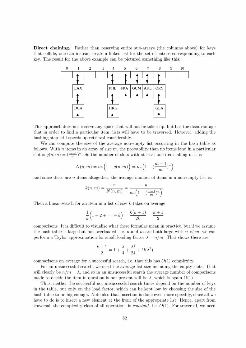
Direct chaining. Rather than reserving entire sub-arrays (the columns above) for keysthat collide, one can instead create a linked list for the set of entries corresponding to eachkey. The result for the above example can be pictured something like this:

LAX

DCA

FRA GCMPHL

HKG

AKL ORY

GLA

0 1 2 3 4 5 6 7 8 9 10

This approach does not reserve any space that will not be taken up, but has the disadvantagethat in order to find a particular item, lists will have to be traversed. However, adding thehashing step still speeds up retrieval considerably.

We can compute the size of the average non-empty list occurring in the hash table asfollows. With n items in an array of size m, the probability than no items land in a particularslot is q(n,m) = (m−1

m )n. So the number of slots with at least one item falling in it is

N(n,m) = m.(

1 − q(n,m))

= m.(

1 − (m − 1

m)n

)

and since there are n items altogether, the average number of items in a non-empty list is:

k(n,m) =n

N(n,m)=

n

m.(

1 − (m−1m )n

) .

Then a linear search for an item in a list of size k takes on average

1

k

(

1 + 2 + · · · + k)

=k(k + 1)

2k=

k + 1

2

comparisons. It is difficult to visualize what these formulae mean in practice, but if we assumethe hash table is large but not overloaded, i.e. n and m are both large with n � m, we canperform a Taylor approximation for small loading factor λ = n/m. That shows there are

k + 1

2= 1 +

λ

4+

λ2

24+ O(λ3)

comparisons on average for a successful search, i.e. that this has O(1) complexity.For an unsuccessful search, we need the average list size including the empty slots. That

will clearly be n/m = λ, and so in an unsuccessful search the average number of comparisonsmade to decide the item in question is not present will be λ, which is again O(1).

Thus, neither the successful nor unsuccessful search times depend on the number of keysin the table, but only on the load factor, which can be kept low by choosing the size of thehash table to be big enough. Note also that insertion is done even more speedily, since all wehave to do is to insert a new element at the front of the appropriate list. Hence, apart fromtraversal, the complexity class of all operations is constant , i.e. O(1). For traversal, we need

82

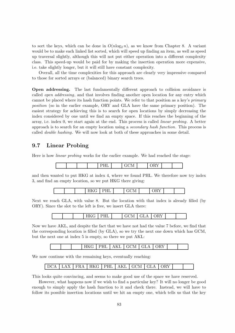
to sort the keys, which can be done in O(nlog2 n), as we know from Chapter 8. A variantwould be to make each linked list sorted, which will speed up finding an item, as well as speedup traversal slightly, although this will not put either operation into a different complexityclass. This speed-up would be paid for by making the insertion operation more expensive,i.e. take slightly longer, but it will still have constant complexity.

Overall, all the time complexities for this approach are clearly very impressive comparedto those for sorted arrays or (balanced) binary search trees.

Open addressing. The last fundamentally different approach to collision avoidance iscalled open addressing , and that involves finding another open location for any entry whichcannot be placed where its hash function points. We refer to that position as a key’s primaryposition (so in the earlier example, ORY and GLA have the same primary position). Theeasiest strategy for achieving this is to search for open locations by simply decreasing theindex considered by one until we find an empty space. If this reaches the beginning of thearray, i.e. index 0, we start again at the end. This process is called linear probing . A betterapproach is to search for an empty location using a secondary hash function. This process iscalled double hashing . We will now look at both of these approaches in some detail.

9.7 Linear Probing

Here is how linear probing works for the earlier example. We had reached the stage:

PHL GCM ORY

and then wanted to put HKG at index 4, where we found PHL. We therefore now try index3, and find an empty location, so we put HKG there giving:

HKG PHL GCM ORY

Next we reach GLA, with value 8. But the location with that index is already filled (byORY). Since the slot to the left is free, we insert GLA there:

HKG PHL GCM GLA ORY

Now we have AKL, and despite the fact that we have not had the value 7 before, we find thatthe corresponding location is filled (by GLA), so we try the next one down which has GCM,but the next one at index 5 is empty, so there we put AKL:

HKG PHL AKL GCM GLA ORY

We now continue with the remaining keys, eventually reaching:

DCA LAX FRA HKG PHL AKL GCM GLA ORY

This looks quite convincing, and seems to make good use of the space we have reserved.However, what happens now if we wish to find a particular key? It will no longer be good

enough to simply apply the hash function to it and check there. Instead, we will have tofollow its possible insertion locations until we hit an empty one, which tells us that the key

83

we were looking for is not present, after all, because it would have been inserted there. Thisis why every hash table that uses open addressing should have at least one empty slot at anytime, and be declared full when only one empty location is left. However, as we shall see,hash tables lose much of their speed advantage if they have a high load factor, so as a matterof policy, many more locations should be kept empty.

So, to find the key AKL, we would first check at index 7, then at 6, and 5, where we aresuccessful. Searching for JFK, on the other hand, we would start with its proper position,given by the value 8, so we would check indices 8, 7, 6, . . . , 1, 0, 10 in that order until wefind an empty space which tells us that JFK is, in fact, not present at all. This looks prettybad at first sight, but bear in mind that we said that we will aim towards keeping the loadfactor at around 50 percent, so there would be many more empty slots which effectively stopany further search.

But this idea brings another problem with it. Suppose we now delete GCM from the tableand then search for AKL again. We would find the array empty at index 6 and stop searching,and therefore wrongly conclude that AKL is not present. This is clearly not acceptable, butequally, we do not wish to have to search through the entire array to be sure that an entry isnot there. The solution is that we reserve another key to mean that a position is empty, butthat it did hold a key at some point. Let us assume that we use the character ‘!’ for that.Then after deleting GCM, the array would be:

DCA LAX FRA HKG PHL AKL ! GLA ORY

and when searching for AKL we would know to continue beyond the exclamation mark. If,on the other hand, we are trying to insert a key, then we can ignore any exclamation marksand fill the position once again. This now does take care of all our problems, although if wedo a lot of deleting and inserting, we will end up with a table which is a bit of a mess. A largenumber of exclamation marks means that we have to keep looking for a long time to find aparticular entry despite the fact that the load factor may not be all that high. This happensif deletion is a frequent operation. In such cases, it may be better to re-fill a new hash tableagain from scratch, or use another implementation.

Search complexity. The complexity of open addressing with linear probing is rather dif-ficult to compute, so we will not attempt to present a full account of it here. If λ is onceagain the load factor of the table, then a successful search can be shown to take 1

2(1 + 11−λ )

comparisons on average, while an unsuccessful search takes approximately 12(1 + 1

(1−λ)2). For

relatively small load factors, this is quite impressive, and even for larger ones, it is not bad.Thus, the hash table time complexity for search is again constant, i.e. O(1).

Clustering. There is a particular problem with linear probing, namely what is known asprimary and secondary clustering . Consider what happens if we try to insert two keys thathave the same result when the hash function is applied to them. Take the above examplewith hash table at the stage where we just inserted GLA:

HKG PHL GCM GLA ORY

If we next try to insert JFK we note that the hash function evaluates to 8 once again. So wekeep checking the same locations we only just checked in order to insert GLA. This seems a

84

rather inefficient way of doing this. This effect is known as primary clustering because thenew key JFK will be inserted close to the previous key with the same primary position, GLA.It means that we get a continuous ‘block’ of filled slots, and whenever we try to insert any keywhich is sent into the block by the hash function, we will have to test all locations until wehit the end of the block, and then make such block even bigger by appending another entryat its end. So these blocks, or clusters, keep growing, not only if we hit the same primarylocation repeatedly, but also if we hit anything that is part of the same cluster. The lasteffect is called secondary clustering . Note that searching for keys is also adversely affected bythese clustering effects.

9.8 Double Hashing

The way to avoid the clustering problems of linear probing is to do something slightly moresophisticated than trying every position to the left until we find an empty one. This is knownas double hashing . We apply a secondary hash function to tell us how many slots to jump tolook for an empty slot if a key’s primary position has been filled already.

Like the primary hash function, there are many possible choices of the secondary hashfunction. In the above example, one thing we could do is take the same number k associatedwith the three-character code, and use the result of integer division by 11, instead of theremainder, as the secondary hash function. However, the resulting value might be bigger than10, so to prevent the jump looping round back to, or beyond, the starting point, we first takethe result of integer division by 11, and then take the remainder this result leaves when againdivided by 11. Thus we would like to use as our secondary hash function h2(n) = (k/11)%11.However, this has yet another problem: it might give zero at some point, and we obviouslycannot test ‘every zeroth location’. An easy solution is to simply make the secondary hashfunction one if the above would evaluate to zero, that is:

h2(n) =

{

(k/11)%11 if (k/11)%11 6= 0,1 otherwise.

The values of this for our example set of keys are given in the following table:

Code PHL ORY GCM HKG GLA AKL FRA LAX DCA BHX

h2(X1X2X3) 4 1 1 3 9 2 6 7 2 3

We then proceed from the position we were in when the first collision occurred:

PHL GCM ORY

with HKG the next key to insert, which gives a collision with PHL. Since h2(HKG) = 3 wenow try every third location to the left in order to find a free slot:

HKG PHL GCM ORY

Note that this did not create a block. When we now try to insert GLA, we once again findits primary location blocked by ORY. Since h2(GLA) = 9, we now try every ninth location.Counting to the left from ORY, that gets us (starting again from the back when we reach thefirst slot) to the last location overall:

85

HKG PHL GCM ORY GLA .

Note that we still have not got any blocks, which is good. Further note that most keys whichshare the same primary location with ORY and GLA will follow a different route when tryingto find an empty slot, thus avoiding primary clustering. Here is the result when filling thetable with the remaining keys given:

HKG DCA PHL FRA GCM AKL ORY LAX GLA

Our example is too small to show convincingly that this method also avoids secondary clus-tering, but in general it does.

It is clear that the trivial secondary hash function h2(n) = 1 reduces this approach to thatof linear probing. It is also worth noting that, in both cases, proceeding to secondary positionsto the left is merely a convention – it could equally well be to the right – but obviously it hasto be made clear which direction has been chosen for a particular hash table.

Search complexity. The efficiency of double hashing is even more difficult to computethan that of linear probing, and therefore we shall just give the results without a derivation.With load factor λ, a successful search requires (1/λ) ln(1/(1 − λ)) comparisons on average,and an unsuccessful one requires 1/(1 − λ). Note that it is the natural logarithm (to basee = 2.71828 . . .) that occurs here, rather than the usual logarithm to base 2. Thus, the hashtable time complexity for search is again constant, i.e. O(1).

9.9 Choosing good hash functions

In principle, any convenient function can be used as a primary hash function. However,what is important when choosing a good hash function is to make sure that it spreads thespace of possible keys onto the set of hash table indices as evenly as possible. Secondly, it isadvantageous if any potential clusters in the space of possible keys are broken up (somethingthat the remainder in a division will not do), because in that case we could end up witha ‘continuous run’ and associated clustering problems in the hash table. Therefore, whendefining hash functions of strings of characters, it is never a good idea to make the last (oreven the first) few characters decisive.

When choosing secondary hash functions, in order to avoid primary clustering, one hasto make sure that different keys with the same primary position give different results whenthe secondary hash function is applied. Secondly, one has to be careful to ensure that thesecondary hash function cannot result in a number which has a common divisor with thesize of the hash table. For example, if the hash table has size 10, and we get a secondaryhash function which gives 2 (or 4, 6 or 8) as a result, then only half of the locations will bechecked, which might result in failure (an endless loop, for example) while the table is stillhalf empty. Even for large hash tables, this can still be a problem if the secondary hash keyscan be similarly large. A simple remedy for this is to always make the size of the hash tablea prime number.

9.10 Complexity of hash tables

The following table gives the average number of locations that have to be checked to conductsuccessful and unsuccessful searches in hash tables with different collision handling strategies,

86

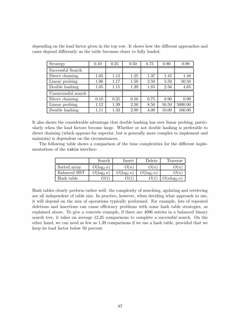
depending on the load factor given in the top row. It shows how the different approaches andcases depend differently as the table becomes closer to fully loaded.

Strategy 0.10 0.25 0.50 0.75 0.90 0.99

Successful Search

Direct chaining 1.05 1.12 1.25 1.37 1.45 1.48

Linear probing 1.06 1.17 1.50 2.50 5.50 50.50

Double hashing 1.05 1.15 1.39 1.85 2.56 4.65

Unsuccessful search

Direct chaining 0.10 0.25 0.50 0.75 0.90 0.99

Linear probing 1.12 1.39 2.50 8.50 50.50 5000.00

Double hashing 1.11 1.33 2.00 4.00 10.00 100.00

It also shows the considerable advantage that double hashing has over linear probing, partic-ularly when the load factors become large. Whether or not double hashing is preferable todirect chaining (which appears far superior, but is generally more complex to implement andmaintain) is dependent on the circumstances.

The following table shows a comparison of the time complexities for the different imple-mentations of the table interface:

Search Insert Delete Traverse

Sorted array O(log2 n) O(n) O(n) O(n)

Balanced BST O(log2 n) O(log2 n) O(log2 n) O(n)

Hash table O(1) O(1) O(1) O(nlog2 n)

Hash tables clearly perform rather well: the complexity of searching, updating and retrievingare all independent of table size. In practice, however, when deciding what approach to use,it will depend on the mix of operations typically performed. For example, lots of repeateddeletions and insertions can cause efficiency problems with some hash table strategies, asexplained above. To give a concrete example, if there are 4096 entries in a balanced binarysearch tree, it takes on average 12.25 comparisons to complete a successful search. On theother hand, we can need as few as 1.39 comparisons if we use a hash table, provided that wekeep its load factor below 50 percent.

87

Chapter 10

Graphs

Often it is useful to represent information in a more general graphical form than consideredso far, such as the following representation of the distances between towns:

Edinburgh

Newcastle

Manchester

London

Exeter

110

Glasgow44

215

Swansea

80

157

117

286

168

Birmingham

119

198

With similar structures (maybe leaving out the distances, or replacing them by somethingelse), we could represent many other situations, like an underground tunnel network, or anetwork of pipes (where the number label might give the pipe diameters), or a railway map,or an indication of which cities are linked by flights, or ferries, or political alliances. Even ifwe assume it is a network of paths or roads, the numbers do not necessarily have to representdistances, they might be an indication for how long it takes to cover the distance in questionon foot, so a given distance up a steep hill would take longer than on even ground.

There is much more that can be done with such a picture of a situation than just readingoff which place is directly connected with another place: For example, we can ask ourselves

88

whether there is a way of getting from A to B at all, or what is the shortest path, or whatwould be the shortest set of pipes connecting all the locations. There is also the famousTravelling Salesman Problem which involves finding the shortest route through the structurethat visits each city precisely once.

10.1 Graphs

The kind of structure in the above figure is known formally as a graph. A graph consists ofa series of nodes (also called vertices or points), displayed as nodes, and edges (also calledlines, links or, in directed graphs, arcs), displayed as connections between the nodes. Thereexists quite a lot of terminology that allows us to specify graphs precisely:

If there are labels on the edges (usually non-negative real numbers) we say that the graphis weighted . We distinguish between directed and undirected graphs. For the former (alsocalled digraphs), each edge comes with a direction (usually indicated by an arrow). Think ofthem as representing roads, where some roads may be one-way only. Or think of the numberscoming with them as something that applies to travel in one-way only: such as going up ahill which will take longer than coming down. An example of an unweighted digraph is:

A

B C

D

E

and an example of a weighted digraph, because it has labels on its edges, is:

4

2 2

6

1

3

1 1

2

2

3

2

E

D

C

A

B

In undirected graphs, we assume that every edge can be viewed as going both ways, that is,an edge between A and B goes from A to B as well as from B to A. The first graph given atthe beginning of this chapter is weighted and undirected.

A path is a sequence of nodes or vertices v1, v2, . . . , vn such that vi and vi+1 are connectedby an edge for all 1 ≤ i ≤ n−1. Note that in a directed graph, the edge from vi to vi+1 is theone which has the corresponding direction. A circle is a non-empty path whose first vertexis the same as its last vertex. An undirected graph is connected if every pair of vertices hasa path connecting them.

For directed graphs, the notion of connectedness has two distinct versions: We say thata digraph is weakly connected if for every two vertices A and B there is either a path fromA to B or a path from B to A. We say it is strongly connected if there are paths leadingboth ways. So, in a weakly connected digraph, there may be two vertices i and j such that

89

there exists no path from i to j. A path is simple if no vertex appears on it twice (with theexception of a circle, where the first and last vertex may be the same – this is because wehave to ‘cut open’ the circle at some point to get a path, so this is inevitable).

A graph is said to be simple if it has no self-loops (i.e. edges connected at both ends tothe same vertex) and no more than one edge connecting any pair of vertices. The remainderof this Chapter will assume that, which is sufficient for many practical applications.

A graph clearly has many properties similar to a tree. In fact, any tree can be viewedas a simple graph of a particular kind, namely one that is connected and contains no circles.Because a graph, unlike a tree, does not come with a natural ‘starting point’ from whichthere is a unique path to each vertex, it does not make sense to speak of parents and childrenin a graph. Instead, if two vertices A and B are connected by an edge e, we say that theyare neighbours, and the edge connecting them is said to be incident to A and B. Two edgesthat have a vertex in common (for example, one connecting A and B and one connecting Band C) are said to be adjacent .

10.2 Implementing graphs

All the data structures we have considered so far were designed to hold certain information,and we wanted to perform certain actions on them which mostly centred around inserting newitems, deleting particular items, searching for particular items, and sorting the collection. Atno time was there ever a connection between all the items represented, apart from the order inwhich their keys appeared. Moreover, that connection was never something that was inherentin the structure and that we therefore tried to represent somehow – it was just a propertythat we used to store the items in a way which made sorting and searching quicker. Now, onthe other hand, it is the connections that are the crucial information we need to encode inthe data structure. We are given a structure which comes with specified connections, and weneed to design an implementation that efficiently keeps track of them.

Array-based implementation. The first underlying idea for array-based implementationsis that we can conveniently rename the vertices of the graph so that they are labelled bynon-negative integer indices, say from 0 to n − 1, if they do not have these labels already.However, this only works if the graph is given explicitly, that is, if we know in advance howmany vertices there will be, and which pairs will have edges between them. Then we only needto keep track of which vertex has an edge to which other vertex, and, for weighted graphs,what the weights on the edges are. For unweighted graphs, we can do this quite easily in ann×n two-dimensional array adj, also called a matrix , the so-called adjacency matrix . In thecase of weighted graphs, we instead have the n×n weight matrix weights. The array/matrixrepresentations for the two example graphs shown above are then:

A B C D E

0 1 2 3 4

A 0 0 1 0 1 0

B 1 0 0 1 0 0

C 2 1 0 0 0 1

D 3 0 0 1 0 1

E 4 0 0 0 0 0

A B C D E

0 1 2 3 4

A 0 0 1 ∞ 4 ∞B 1 2 0 2 2 6

C 2 ∞ 3 0 2 1

D 3 ∞ ∞ ∞ 0 1

E 4 ∞ ∞ 3 2 0

90

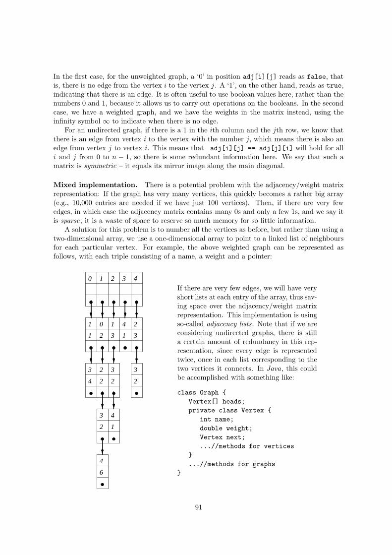
In the first case, for the unweighted graph, a ‘0’ in position adj[i][j] reads as false, thatis, there is no edge from the vertex i to the vertex j. A ‘1’, on the other hand, reads as true,indicating that there is an edge. It is often useful to use boolean values here, rather than thenumbers 0 and 1, because it allows us to carry out operations on the booleans. In the secondcase, we have a weighted graph, and we have the weights in the matrix instead, using theinfinity symbol ∞ to indicate when there is no edge.

For an undirected graph, if there is a 1 in the ith column and the jth row, we know thatthere is an edge from vertex i to the vertex with the number j, which means there is also anedge from vertex j to vertex i. This means that adj[i][j] == adj[j][i] will hold for alli and j from 0 to n − 1, so there is some redundant information here. We say that such amatrix is symmetric – it equals its mirror image along the main diagonal.

Mixed implementation. There is a potential problem with the adjacency/weight matrixrepresentation: If the graph has very many vertices, this quickly becomes a rather big array(e.g., 10,000 entries are needed if we have just 100 vertices). Then, if there are very fewedges, in which case the adjacency matrix contains many 0s and only a few 1s, and we say itis sparse, it is a waste of space to reserve so much memory for so little information.

A solution for this problem is to number all the vertices as before, but rather than using atwo-dimensional array, we use a one-dimensional array to point to a linked list of neighboursfor each particular vertex. For example, the above weighted graph can be represented asfollows, with each triple consisting of a name, a weight and a pointer:

0 1 2 3 4

1

1

3

4

0

2

2

2

3

2

4

6

1

3

3

2

4

1

4

1

2

3

3

2

If there are very few edges, we will have veryshort lists at each entry of the array, thus sav-ing space over the adjacency/weight matrixrepresentation. This implementation is usingso-called adjacency lists. Note that if we areconsidering undirected graphs, there is stilla certain amount of redundancy in this rep-resentation, since every edge is representedtwice, once in each list corresponding to thetwo vertices it connects. In Java, this couldbe accomplished with something like:

class Graph {

Vertex[] heads;

private class Vertex {

int name;

double weight;

Vertex next;

...//methods for vertices

}

...//methods for graphs

}

91

Pointer-based implementation. The pointer -based implementation for binary trees (whichin turn generalizes linked lists) can be generalized for graphs. In a language such as Java, aclass Graph might have the following as an internal class:

class Vertex {

string name;

Vertex[] neighbours;

double[] weights;

}

When we create each vertex, we allocate an array neighbours big enough to accommodate(pointers to) all its neighbours, and (for weighted graphs) an equal sized array weights toaccommodate the associated weights. We then place the neighbours of the vertex into thosearrays in some arbitrary order. Any non-needed entries in the neighbours array will holda null pointer as usual. For example, the above weighted graph would be represented asfollows, with each weight following the associated pointer:

0

2

3

4

1 4 1

3 2 1

2 3

1 6222

10.3 Subgraphs, subdivisions and minors

Many important theorems about graphs rely on formal definitions of the relations betweenthem, so we now consider the relevant concepts. Two graphs are said to be isomorphic ifthey contain the same number of vertices with the same pattern of adjacency, i.e. there isa bijection between their vertices which preserves the adjacency relations. A subgraph of agraph G is defined as any graph that has a vertex set which is a subset of that of G, withadjacency relations which are a subset of those of G. Conversely, a supergraph of a graph Gis defined as a graph of which G is a subgraph. Finally, a graph G is said to contain anothergraph H if there exists a subgraph of G that is either H or isomorphic to H.

A subdivision of an edge e with endpoints u and v is simply the pair of edges e1, withendpoints u and w, and e2, with endpoints w and v, for some new vertex w. The reverseoperation of smoothing removes a vertex w with exactly two edges e1 and e2, leaving an edgee connecting the two adjacent vertices u and v:

92

Then a subdivision of a graph G can be defined as a graph resulting from the subdivision ofedges in G. Two graphs G and H can then be defined as being homeomorphic if there is agraph isomorphism from some subdivision of G to some subdivision of H.

An edge contraction removes an edge from a graph and merges the two vertices previouslyconnected by it. This can lead to multiple edges between a pair of vertices, or self-loops whichare edges that connect a vertex to itself. These are not allowed in simple graphs, in whichcase they need to be deleted. Then an undirected graph H is said to be a minor of anotherundirected graph G if a graph isomorphic to H can be obtained from G by contracting someedges, deleting some edges, and deleting some isolated vertices.

10.4 Planarity

A planar graph is a graph that can be embeded in a plane. In other words, it can be drawnon a sheet of paper in such a way that no edges cross each other. This is important inapplications such as printed circuit design.

Note that it is clearly possible for planar graphs to be drawn in such a way that theiredges do cross each other, but the crucial thing is that they can be transformed (by movingvertices and/or deforming the edges) into a form without any edges crossing. For example,the following three diagrams all represent the same planar graph:

This graph is the fully connected graph with four vertices, known as K4. Clearly all sub-graphs of this will also be planar.

It is actually quite difficult to formulate general algorithms for determining whether agiven graph is planar. For small graphs, it is easy to check systematically that there are nopossible vertex repositionings or edge deformations that will bring the graph into explicitlyplanar form. Two slightly larger graphs than K4 that can be shown to be non-planar in thisway are the fully connected graph with five vertices, known as K5, and the graph with threevertices fully connected to three other vertices, known as K3,3:

Clearly, any larger graph that contains one of these two non-planar graphs as a subgraph mustalso be non-planar iteslf, and any subdivision or smoothing of edges will have no effect on

93

the planarity. In fact, it can be proved that these two graphs form the basis of some usefultheorems about planarity. The most well-known of these is Kuratowski’s theorem which statesthat “a finite graph is planar if and only if it does not contain a subgraph that is homeomorphicto, or a subdivision of, K5 or K3,3”. Another, based on the concept of minors, is Wagner’stheorem which states that “a finite graph is planar if and only if it does not have K5 or K3,3

as a minor”.A good general approach for testing planarity is therefore to search for subgraphs of the

given graph that can be transformed into K5 or K3,3. This is not entirely straightforward,but algorithms do exist which allow a graph with n vertices to be tested for planarity withtime complexity O(n). Exercise: find out exactly how these algorithms work.

10.5 Traversals – systematically visiting all vertices

In order to traverse a graph, i.e. systematically visit all its vertices, we clearly need a strategyfor exploring graphs which guarantees that we do not miss any edges or vertices. Because,unlike trees, graphs do not have a root vertex, there is no natural place to start a traversal,and therefore we assume that we are given, or randomly pick, a starting vertex i. There aretwo strategies for performing graph traversal.

The first is known as breadth first traversal : We start with the given vertex i. Then wevisit its neighbours one by one (which must be possible no matter which implementation weuse), placing them in an initially empty queue. We then remove the first vertex from thequeue and one by one put its neighbours at the end of the queue. We then visit the nextvertex in the queue and again put its neighbours at the end of the queue. We do this untilthe queue is empty.

However, there is no reason why this basic algorithm should ever terminate. If there is acircle in the graph, like A, B, C in the first unweighted graph above, we would revisit a vertexwe have already visited, and thus we would run into an infinite loop (visiting A’s neighboursputs B onto the queue, visiting that (eventually) gives us C, and once we reach C in the queue,we get A again). To avoid this we create a second array done of booleans, where done[j] istrue if we have already visited the vertex with number j, and it is false otherwise. In theabove algorithm, we only add a vertex j to the queue if done[j] is false. Then we mark itas done by setting done[j] = true. This way, we will not visit any vertex more than once,and for a finite graph, our algorithm is bound to terminate. In the example we are discussing,breadth first search starting at A might yield: A, B, D, C, E.

To see why this is called breadth first search, we can imagine a tree being built up in thisway, where the starting vertex is the root, and the children of each vertex are its neighbours(that haven’t already been visited). We would then first follow all the edges emanating fromthe root, leading to all the vertices on level 1, then find all the vertices on the level below,and so on, until we find all the vertices on the ‘lowest’ level.

The second traversal strategy is known as depth first traversal : Given a vertex i to startfrom, we now put it on a stack rather than a queue (recall that in a stack, the next item tobe removed at any time is the last one that was put on the stack). Then we take it fromthe stack, mark it as done as for breadth first traversal, look up its neighbours one after theother, and put them onto the stack. We then repeatedly pop the next vertex from the stack,mark it as done, and put its neighbours on the stack, provided they have not been marked asdone, just as we did for breadth first traversal. For the example discussed above, we might

94

get (again starting from A): A, B, C, E, D. Again, we can see why this is called depth firstby formulating the traversal as a search tree and looking at the order in which the items areadded and processed.

Note that with both breadth first and depth first, the order of the vertices depends onthe implementation. There is no reason why A’s neighbour B should be visited before D inthe example. So it is better to speak of a esult of depth first or breadth first traversal, ratherthan of the result. Note also that the only vertices that will be listed are those in the sameconnected component as A. If we have to ensure that all vertices are visited, we may needto start the traversal process with a number of different starting vertices, each time choosingone that has not been marked as done when the previous traversal terminated.

Exercises: Write algorithms, in pseudocode, to (1) visit all nodes of a graph, and (2) decidewhether a given graph is connected or not. For (2) you will actually need two algorithms,one for the strong notion of connectedness and another for the weak notion.

10.6 Shortest paths – Dijkstra’s algorithm

A common graph based problem is that we are given a weighted digraph with edges labelled bynon-negative numbers and need to answer the following question: For two particular vertices,what is the shortest route from one to the other?

Here, by “shortest route” we mean a path which, when we add up the weights along itsedges, gives the smallest overall weight for the path. This number is called the length of thepath. Thus, a shortest path is one with minimal length. Note that there need not be a uniqueshortest path, since several paths might have the same length. In a disconnected graph therewill not be a path between vertices in different components, but we can take care of this byusing ∞ once again to stand for “no path at all”.

Note that the weights do not necessarily have to correspond to distances; they could, forexample, be time (in which case we could speak of “quickest paths”) or money (in which casewe could speak of “cheapest paths”), among other possibilities. By considering “abstract”graphs in which the numerical weights are left uninterpreted, we can take care of all suchsituations and others. But notice that we do need to restrict the edge weights to be non-negative numbers, because if there are negative numbers and cycles, we can have increasinglylong paths with lower and lower costs, and no path with minimal cost.

Applications of shortest-path algorithms include internet packet routing (because, if yousend an email message from your computer to someone else, it has to go through variouscomputer routers, until it reaches its final destination), train-ticket reservation systems (thatneed to figure out the best connecting stations), and driving route finders (that need to findan optimum route in some sense).

Dijkstra’s algorithm. In turns out that, if we want to compute the shortest path froma given start node s to a given end node z, it is actually most convenient to compute theshortest paths from s to all other nodes, not just the given node z that we are interestedin. Given the start node, Dijkstra’s algorithm computes shortest paths starting from s andending at each possible node. Because the algorithm, although elegant and short, is fairlycomplicated, we shall consider it one component at a time.

Overestimation of shortest paths. We keep an array D of distances indexed by thevertices. The idea is that D[z] will hold the distance of the shortest path from s to z when

95

the algorithm finishes. However, before the algorithm finishes, D[z] is the best overestimatewe currently have of the distance from s to z. We initially set D[s] = 0 and D[z] = ∞ forall vertices z other than the start node s. What the algorithm does is to repeatedly decreasethe overestimates until it is no longer possible to do so. When this happens, the algorithmterminates, and the estimates are now fully constrained and said to be tight .

Improving estimates. The general idea is to look systematically for shortcuts. Supposethat, for two given vertices u and z, it happens that D[u] + weight[u][z] < D[z]. Then thereis a way of going from s to u and then to z whose total length is smaller than the currentoverestimate D[z] of the distance from s to z, and hence we can replace D[z] by this betterestimate. This corresponds to the code fragment

if ( D[u] + weight[u][z] < D[z] )

D[z] = D[u] + weight[u][z]

of the full algorithm given below. The problem now is how to systematically apply thisimprovement so that (1) we eventually get the tight estimates promised above, and (2) thisis done efficiently.

Dijkstra’s algorithm, Version 1. The first version of the algorithm is not as efficientas it could be, but it is relatively simple and certainly correct. (It is always a good idea tostart with an inefficient simple algorithm, so that the results from it can be used to check theoperation of a more complex efficient algorithm.) The general idea is that, at each stage ofthe algorithm’s operation, if an entry D[u] of the array D has the minimal value among all thevalues recorded in D, then the overestimate D[u] is actually tight, because the improvementalgorithm discussed above cannot possibly find a shortcut.

The following algorithm implements that idea:

// Input: A directed graph with weight matrix ‘weight’ and

// a start vertex ‘s’.

// Output: An array ‘D’ as explained above.

// We begin by buiding the overestimates.

D[s] = 0 // The shortest path from s to itself has length zero.

for ( each vertex z of the graph ) {

if ( z is not the start vertex s )

D[z] = infinity // This is certainly an overestimate.

}

// We use an auxiliary array ‘tight’ indexed by the vertices,

// that records for which nodes the shortest path estimates

// are ‘‘known’’ to be tight by the algorithm.

for ( each vertex z of the graph ) {

tight[z] = false

}

96

// We now repeatedly update the arrays ‘D’ and ‘tight’ until

// all entries in the array ‘tight’ hold the value true.

repeat as many times as there are vertices in the graph {

find a vertex u with tight[u] false and minimal estimate D[u]

tight[u] = true

for ( each vertex z adjacent to u )

if ( D[u] + weight[u][z] < D[z] )

D[z] = D[u] + weight[u][z] // lower overestimate exists

}

// At this point, all entries of array ‘D’ hold tight estimates.

It is clear that when this algorithm finishes, the entries of D will still hold overestimates ofthe lengths of the shortest paths. What is perhaps not so clear is why these estimates areactually tight, i.e. hold the minimal path lengths. In order to understand why, first noticethat an initial sub-path of a shortest path is itself a shortest path. To see this, suppose thatyou wish to navigate from a vertex s to a vertex z, and that the shortest path from s toz happens to go through a certain vertex u. Then your path from s to z can be split intotwo paths, one going from s to u (an initial sub-path) and the other going from u to z (afinal sub-path). Given that the whole, unsplit path is a shortest path from s to z, the initialsub-path has to be a shortest path from s to u, for if not, then you could shorten your pathfrom s to z by replacing the initial sub-path to u by a shorter path, which would not only givea shorter path from s to u but also from s to the final destination z. Now it follows that forany start vertex, there is a tree of shortest paths from that vertex to all other vertices. Thereason is that shortest paths cannot have cycles. Implicitly, Dijkstra’s algorithm constructsthis tree starting from the root, that is, the start vertex.

If, as tends to be the case in practice, we also wish to compute the route of shortest path,rather than just its length, we also need to introduce a second array pred to keep track ofthe ’predecessor’ or ‘previous vertex’ of each vertex, so that the path can be followed backfrom the end point to the start point. The algorithm can clearly also be adapted to workwith non-weighted graphs by assigning a suitable weight matrix of 1s for connected verticesand 0s for non-connected vertices.

The time complexity of this algorithm is clearly O(n2) where n is the number of vertices,since there are operations of O(n) nested within the repeat of O(n).

An example. Suppose we want to compute the shortest path from A (node 0) to E (node4) in the weighted graph we looked at before:

4

2 2

6

1

3

1 1

2

2

3

2

E

D

C

A

B

97

An implementation of the above algorithm, with some code added to print out the status ofthe intermediate calculations and keep track of predecessors, gives the following output, inwhich“oo” is used to represent the infinity symbol “∞”:

Computing shortest paths from A

|A B C D E

--------+---------------------------------------

D |0 oo oo oo oo

tight |no no no no no

pred. |none none none none none

Vertex A has minimal estimate, and so is tight.

Neighbour B has estimate decreased from oo to 1 taking a shortcut via A.

Neighbour D has estimate decreased from oo to 4 taking a shortcut via A.

|A B C D E

--------+---------------------------------------

D |0 1 oo 4 oo

tight |yes no no no no

pred. |none A none A none

Vertex B has minimal estimate, and so is tight.

Neighbour A is already tight.

Neighbour C has estimate decreased from oo to 3 taking a shortcut via B.

Neighbour D has estimate decreased from 4 to 3 taking a shortcut via B.

Neighbour E has estimate decreased from oo to 7 taking a shortcut via B.

|A B C D E

--------+---------------------------------------

D |0 1 3 3 7

tight |yes yes no no no

pred. |none A B B B

Vertex C has minimal estimate, and so is tight.

Neighbour B is already tight.

Neighbour D has estimate unchanged.

Neighbour E has estimate decreased from 7 to 4 taking a shortcut via C.

|A B C D E

--------+---------------------------------------

D |0 1 3 3 4

tight |yes yes yes no no

pred. |none A B B C

98

Vertex D has minimal estimate, and so is tight.

Neighbour E has estimate unchanged.

|A B C D E

--------+---------------------------------------

D |0 1 3 3 4

tight |yes yes yes yes no

pred. |none A B B C

Vertex E has minimal estimate, and so is tight.

Neighbour C is already tight.

Neighbour D is already tight.

|A B C D E

--------+---------------------------------------

D |0 1 3 3 4

tight |yes yes yes yes yes

pred. |none A B B C

End of Dijkstra’s computation.

A shortest path from A to E is: A B C E.

Once it is clear what is happening at each stage, it is usually more convenient to adopt ashorthand notation that allows the whole process to be represented in a single table. Forexample, using a “*” to represent tight, the distance, predecessor and status for each node ateach stage of the above example can be listed more concisely as follows:

Stage | A B C D E

-------+-------------------------------------------

1 | 0 oo oo oo oo

2 | 0* 1 A oo 4 A oo

3 | 0* 1* A 3 B 3 B 7 B

4 | 0* 1* A 3* B 3 B 4 C

5 | 0* 1* A 3* B 3* B 4 C

6 | 0* 1* A 3* B 3* B 4* C

A shortest path from A to E is: A B C E.

Dijkstra’s algorithm, Version 2. The time complexity of Dijkstra’s algorithm can beimproved by making use of a priority queue (e.g., a binary heap tree) to keep track of whichnode’s distance estimate becomes tight next. Here it is convenient to use the convention thatlower numbers have higher priority. The previous algorithm then becomes:

99

// Input: A directed graph with weight matrix ‘weight’ and

// a start vertex ‘s’.

// Output: An array ‘D’ as explained above.

// We begin by buiding the overestimates.

D[s] = 0 // The shortest path from s to itself has length zero.

for ( each vertex z of the graph ) {

if ( z is not the start vertex s )

D[z] = infinity // This is certainly an overestimate.

}

// Then we set up a priority queue based on the overestimates.

Create a priority queue containing all the vertices of the graph,

with the entries of D as the priorities

// Then we implicitly build the path tree discussed above.

while ( priority queue is not empty ) {

// The next vertex of the path tree is called u.

u = remove vertex with smallest priority from queue

for ( each vertex z in the queue which is adjacent to u ) {

if ( D[u] + weight[u][z] < D[z] ) {

D[z] = D[u] + weight[u][z] // lower overestimate exists

Change the priority of vertex z in queue to D[z]

}

}

}

// At this point, all entries of array ‘D’ hold tight estimates.

If the priority queue is implemented as a binary heap tree, initializing D and using heapify tocreate the priority queue both have complexity O(n), where n is the number of vertices of thegraph, and that is negligible compared to the rest of the algorithm. Then removing verticesand changing the priorities of elements in the priority queue require some rearrangement ofthe heap tree by “bubbling up”, and that takes O(log2 n) steps, because that is the maximumheight of the tree. Removals happen O(n) times, and priority changes happen O(e) times,where e is the number of edges in the graph, so the cost of maintaining the queue and updatingD is O((e + n)log2 n). Thus, the total time complexity of this form of the second version ofDijkstra’s algorithm is O((e+n)log2 n). Using a Fibonacci heap for the priority queue is ableto improve this further to O(e + nlog2 n).

In a fully connected graph, the number of edges e will be O(n2), and hence the timecomplexity of this algorithm is O(n2log2 n) or O(n2) depending on which kind of priorityqueue is used. So, in that case, the time complexity is actually greater than or equal to theprevious simpler O(n2) algorithm. However, in practice, many graphs tend to be much more

100

sparse with e = O(n). That is, there are usually not many more edges than vertices, and inthis case the time complexity for both priority queue versions is O(nlog2 n), which is a clearimprovement over the previous O(n2) algorithm.

10.7 Shortest paths – Floyd’s algorithm

If we are not only interested in finding the shortest path from one specific vertex to allthe others, but the shortest paths between every pair of vertices, we could, of course, applyDijkstra’s algorithm to every starting vertex. But there is actually a simpler way of doing this,known as Floyd’s algorithm. This keeps a matrix ‘distance’ which contains the overestimatesof the shortest paths between every pair of vertices, and then systematically decreases theoverestimates using the same shortcut idea as above. If we also wish to keep track of theroutes of the shortest paths, rather than just their lengths, we need to introduce a secondmatrix ‘predecessor’ that keeps track of all the ‘previous vertices’.

In the algorithm below, we attempt to decrease the estimate of the distance from eachvertex s to each vertex z by going systematically via each possible vertex u to see whetherthat is a shortcut; and if it is, the overestimate of the distance is decreased to the smalleroverestimate, and the predecessor updated:

// Store initial estimates and predecessors.

for ( each vertex s ) {

for ( each vertex z ) {

distance[s][z] = weight[s][z]

predecessor[s][z] = s

}

}

// Improve them by considering all possible shortcuts u.

for ( each vertex u ) {

for ( each vertex s ) {

for ( each vertex z ) {

if ( distance[s][u]+distance[u][z] < distance[s][z] ) {

distance[s][z] = distance[s][u]+distance[u][z]

predecessor[s][z] = predecessor[u][z]

}

}

}

}

As with Dijkstra’s algorithm, this can easily be adapted to the case of non-weighted graphsby assigning a suitable weight matrix of 0s and 1s.

The time complexity here is clearly O(n3), since it involves three nested for loops of O(n).This is the same complexity as running the O(n2) Dijkstra’s algorithm once for each of the npossible starting vertices. In general, however, Floyd’s algorithm will be faster than Dijkstra’s,even though they are both in the same complexity class, because the former performs fewer

101

instructions in each run through the loops. However, if the graph is sparse with e = O(n),then multiple runs of Dijkstra’s algorithm can be made to perform with time complexityO(n2log2 n), and be faster than Floyd’s algorithm.

An example. Suppose we want to compute the lengths of the shortest paths between allvertices in the following undirected weighted graph:

We start with distance matrix based on the connection weights, and trivial predecessors:

Start

A B C D E

A 0 1 14 4 ∞B 1 0 ∞ ∞ 2

C 14 ∞ 0 8 10

D 4 ∞ 8 0 1

E ∞ 2 10 1 0

A B C D E

A A A A A A

B B B B B B

C C C C C C

D D D D D D

E E E E E E

Then for each vertex in turn we test whether a shortcut via that vertex reduces any of thedistances, and update the distance and predecessor arrays with any reductions found. Thefive steps, with the updated entries in quotes, are as follows::

A :

A B C D E

A 0 1 14 4 ∞B 1 0 ‘15’ ‘5’ 2

C 14 ‘15’ 0 8 10

D 4 ‘5’ 8 0 1

E ∞ 2 10 1 0

A B C D E

A A A A A A

B B B ‘A’ ‘A’ B

C C ‘A’ C C C

D D ‘A’ D D D

E E E E E E

B :

A B C D E

A 0 1 14 4 ‘3’

B 1 0 15 5 2

C 14 15 0 8 10

D 4 5 8 0 1

E ‘3’ 2 10 1 0

A B C D E

A A A A A ‘B’

B B B A A B

C C A C C C

D D A D D D

E ‘B’ E E E E

C :

A B C D E

A 0 1 14 4 3

B 1 0 15 5 2

C 14 15 0 8 10

D 4 5 8 0 1

E 3 2 10 1 0

A B C D E

A A A A A B

B B B A A B

C C A C C C

D D A D D D

E B E E E E

102

D :

A B C D E

A 0 1 ‘12’ 4 3

B 1 0 ‘13’ 5 2

C ‘12’ ‘13’ 0 8 ‘9’

D 4 5 8 0 1

E 3 2 ‘9’ 1 0

A B C D E

A A A ‘D’ A B

B B B ‘D’ A B

C ‘D’ A C C ‘D’

D D A D D D

E B E ‘D’ E E

E :

A B C D E

A 0 1 12 4 3

B 1 0 ‘11’ ‘3’ 2

C 12 ‘11’ 0 8 9

D 4 ‘3’ 8 0 1

E 3 2 9 1 0

A B C D E

A A A D A B

B B B D ‘E’ B

C D ‘E’ C C D

D D ‘E’ D D D

E B E D E E

The algorithm ends with the array of shortest distances and the array of associated prede-cessors. So the shortest distance from C to B is 11, and the predecessors of B are E, then D,then C, giving the path C D E B. Note that updating a distance does not necessarily meanupdating the associated predecessor – for example, when introducing D as a shortcut betweenC and B, the predecessor of B remains A.

10.8 Minimal spanning trees

We now move on to another common graph-based problem. Suppose you have been given aweighted undirected graph such as the following:

A

B C

D

E F

15

6

3

6

6

4

2

5

5

We could think of the vertices as representing houses, and the weights as the distances betweenthem. Now imagine that you are tasked with supplying all these houses with some commoditysuch as water, gas, or electricity. For obvious reasons, you will want to keep the amount ofdigging and laying of pipes or cable to a minimum. What is the best pipe or cable layout(that is, the one with the shortest length overall) that you can find?

Obviously, we will have to choose some of the edges to dig along, but not all of them. Forexample, if we have already chosen the edge between A and D, and the one between B andD, then there is no reason to also have the one between A and B. More generally, it is clearthat we want to avoid circles. Also, assuming that we have only one feeding-in point (it is ofno importance which of the vertices that is), we need the whole layout to be connected . Wehave seen already that a connected graph without circles is a tree.

103

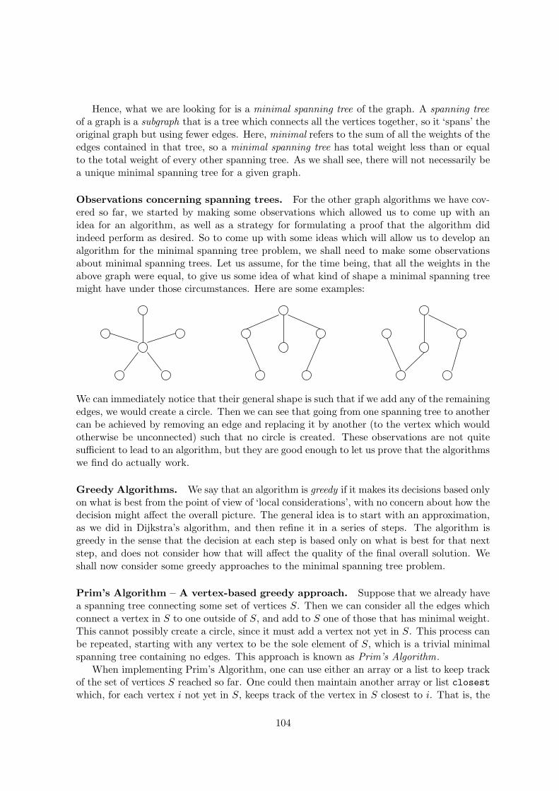
Hence, what we are looking for is a minimal spanning tree of the graph. A spanning treeof a graph is a subgraph that is a tree which connects all the vertices together, so it ‘spans’ theoriginal graph but using fewer edges. Here, minimal refers to the sum of all the weights of theedges contained in that tree, so a minimal spanning tree has total weight less than or equalto the total weight of every other spanning tree. As we shall see, there will not necessarily bea unique minimal spanning tree for a given graph.

Observations concerning spanning trees. For the other graph algorithms we have cov-ered so far, we started by making some observations which allowed us to come up with anidea for an algorithm, as well as a strategy for formulating a proof that the algorithm didindeed perform as desired. So to come up with some ideas which will allow us to develop analgorithm for the minimal spanning tree problem, we shall need to make some observationsabout minimal spanning trees. Let us assume, for the time being, that all the weights in theabove graph were equal, to give us some idea of what kind of shape a minimal spanning treemight have under those circumstances. Here are some examples:

We can immediately notice that their general shape is such that if we add any of the remainingedges, we would create a circle. Then we can see that going from one spanning tree to anothercan be achieved by removing an edge and replacing it by another (to the vertex which wouldotherwise be unconnected) such that no circle is created. These observations are not quitesufficient to lead to an algorithm, but they are good enough to let us prove that the algorithmswe find do actually work.

Greedy Algorithms. We say that an algorithm is greedy if it makes its decisions based onlyon what is best from the point of view of ‘local considerations’, with no concern about how thedecision might affect the overall picture. The general idea is to start with an approximation,as we did in Dijkstra’s algorithm, and then refine it in a series of steps. The algorithm isgreedy in the sense that the decision at each step is based only on what is best for that nextstep, and does not consider how that will affect the quality of the final overall solution. Weshall now consider some greedy approaches to the minimal spanning tree problem.

Prim’s Algorithm – A vertex-based greedy approach. Suppose that we already havea spanning tree connecting some set of vertices S. Then we can consider all the edges whichconnect a vertex in S to one outside of S, and add to S one of those that has minimal weight.This cannot possibly create a circle, since it must add a vertex not yet in S. This process canbe repeated, starting with any vertex to be the sole element of S, which is a trivial minimalspanning tree containing no edges. This approach is known as Prim’s Algorithm.

When implementing Prim’s Algorithm, one can use either an array or a list to keep trackof the set of vertices S reached so far. One could then maintain another array or list closestwhich, for each vertex i not yet in S, keeps track of the vertex in S closest to i. That is, the

104

vertex in S which has an edge to i with minimal weight. If closest also keeps track of theweights of those edges, we could save time, because we would then only have to check theweights mentioned in that array or list.

For the above graph, starting with S = {A}, the tree is built up as follows:

A

B

E F

C

D

1

A

B

E F

C

D

1

4

A

B

E F

C

D

1

4 2

A

B

E F

C

D

1

4 2

5

A

B

E F

C

D

1

4 2

5

3

It is slightly more challenging to produce a convincing argument that this algorithm reallyworks than it has been for the other algorithms we have seen so far. It is clear that Prim’salgorithm must result in a spanning tree, because it generates a tree that spans all the vertices,but it is not obvious that it is minimal. There are several possible proofs that it is, but noneare straightforward. The simplest works by showing that the set of all possible minimalspanning trees Xi must include the output of Prim’s algorithm.

Let Y be the output of Prim’s algorithm, and X1 be any minimal spanning tree. Thefollowing illustrates such a situation:

We don’t actually need to know what X1 is – we just need to know the properties it mustsatisfy, and then systematically work through all the possibilities, showing that Y is a minimalspanning tree in each case. Clearly, if X1 = Y , then Prim’s algorithm has generated a minimalspanning tree. Otherwise, let e be the first edge added to Y that is not in X1. Then, sinceX1 is a spanning tree, it must include a path connecting the two endpoints of e, and becausecircles are not allowed, there must be an edge in X1 that is not in Y , which we can call f .Since Prim’s algorithm added e rather than f , we know weight(e) ≤ weight(f). Then createtree X2 that is X1 with f replaced by e. Clearly X2 is connected, has the same number ofedges as X1, spans all the vertices, and has total weight no greater than X1, so it must also

105

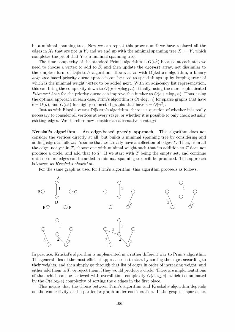
be a minimal spanning tree. Now we can repeat this process until we have replaced all theedges in X1 that are not in Y , and we end up with the minimal spanning tree Xn = Y , whichcompletes the proof that Y is a minimal spanning tree.

The time complexity of the standard Prim’s algorithm is O(n2) because at each step weneed to choose a vertex to add to S, and then update the closest array, not dissimilar tothe simplest form of Dijkstra’s algorithm. However, as with Dijkstra’s algorithm, a binaryheap tree based priority queue approach can be used to speed things up by keeping track ofwhich is the minimal weight vertex to be added next. With an adjacency list representation,this can bring the complexity down to O((e+n)log2 n). Finally, using the more sophisticatedFibonacci heap for the priority queue can improve this further to O(e+nlog2 n). Thus, usingthe optimal approach in each case, Prim’s algorithm is O(nlog2 n) for sparse graphs that havee = O(n), and O(n2) for highly connected graphs that have e = O(n2).

Just as with Floyd’s versus Dijkstra’s algorithm, there is a question of whether it is reallynecessary to consider all vertices at every stage, or whether it is possible to only check actuallyexisting edges. We therefore now consider an alternative strategy:

Kruskal’s algorithm – An edge-based greedy approach. This algorithm does notconsider the vertices directly at all, but builds a minimal spanning tree by considering andadding edges as follows: Assume that we already have a collection of edges T . Then, from allthe edges not yet in T , choose one with minimal weight such that its addition to T does notproduce a circle, and add that to T . If we start with T being the empty set, and continueuntil no more edges can be added, a minimal spanning tree will be produced. This approachis known as Kruskal’s algorithm.

For the same graph as used for Prim’s algorithm, this algorithm proceeds as follows:

A

B

E F

C

D

1 1

2

1

23

1

23 4

1

23 4

5

In practice, Kruskal’s algorithm is implemented in a rather different way to Prim’s algorithm.The general idea of the most efficient approaches is to start by sorting the edges according totheir weights, and then simply go through that list of edges in order of increasing weight, andeither add them to T , or reject them if they would produce a circle. There are implementationsof that which can be achieved with overall time complexity O(elog2 e), which is dominatedby the O(elog2 e) complexity of sorting the e edges in the first place.

This means that the choice between Prim’s algorithm and Kruskal’s algorithm dependson the connectivity of the particular graph under consideration. If the graph is sparse, i.e.

106

the number of edges is not much more than the number of vertices, then Kruskal’s algorithmwill have the same O(nlog2 n) complexity as the optimal priority queue based versions ofPrim’s algorithm, but will be faster than the standard O(n2) Prim’s algorithm. However, ifthe graph is highly connected, i.e. the number of edges is near the square of the number ofvertices, it will have complexity O(n2log2 n) and be slower than the optimal O(n2) versionsof Prim’s algorithm.

10.9 Travelling Salesmen and Vehicle Routing

Note that all the graph algorithms we have considered so far have had polynomial timecomplexity. There are further graph based problems that are even more complex.

Probably the most well known of these is the Travelling Salesman Problem, which involvesfinding the shortest path through a graph which visits each node precisely once. There arecurrently no known polynomial time algorithms for solving this. Since only algorithms withexponential complexity are known, this makes the Travelling Salesman Problem difficult evenfor moderately sized n (e.g., all capital cities). Exercise: write an algorithm in pseudocodethat solves the Travelling Salesman Problem, and determine its time complexity.

A variation of the shortest path problem with enormous practical importance in trans-portation is the Vehicle Routing Problem. This involves finding a series of routes to servicea number of customers with a fleet of vehicles with minimal cost, where that cost may bethe number of vehicles required, the total distance covered, or the total driver time required.Often, for practical instances, there are conflicts between the various objectives, and thereis a trade-off between the various costs which have to be balanced. In such cases, a multi-objective optimization approach is required which returns a Pareto front of non-dominatedsolutions, i.e. a set solutions for which there are no other solutions which are better on allobjectives. Also, in practice, there are usually various constraints involved, such as fixeddelivery time-windows, or limited capacity vehicles, that must be satisfied, and that makesfinding good solutions even more difficult.

Since exact solutions to these problems are currently impossible for all but the smallestcases, heuristic approaches are usually employed, such as evolutionary computation, whichdeliver solutions that are probably good but cannot be proved to be optimal. One popularapproach is to maintain a whole population of solutions, and use simulated evolution bynatural selection to iteratively improve the quality of those solutions. That has the additionaladvantage of being able to generate a whole Pareto front of solutions rather than just a singlesolution. This is currently still a very active research area.

107

Chapter 11

Epilogue

Hopefully the reader will agree that these notes have achieved their objective of introducingthe basic data structures used in computer science, and showing how they can be used inthe design of useful and efficient algorithms. The basic data structures (arrays, lists, stacks,queues, trees) have been employed throughout, and used as the basis of processes such asstoring, sorting and searching which underly many computer science applications. It has beendemonstrated how ideas from combinatorics and probability theory can be used to computethe efficiency of algorithms as a function of problem size. We have seen how considerations ofcomputational efficiency then drive the development of more complex data structures (binarysearch trees, priority queues, hash tables) and associated algorithms. General ideas suchas recursion and divide and conquer have been used repeatedly to provide more efficientalgorithms.

Clearly, these notes have only been able to provide a brief introduction to the topic, andthe algorithms and data structures and efficiency computations discussed have been relativelysimple examples. However, having a good understanding of these fundamental ideas allowsthem to be easily expanded and elaborated to deal with the more complex applications thatwill inevitably arise in the future.

108

Appendix A

Some Useful Formulae

The symbols a, b, c, r and s represent real numbers, m and n are positive integers, and indicesi and j are non-negative integers.

A.1 Binomial formulae

(a + b)2 = a2 + 2ab + b2 (a + b)(a − b) = a2 − b2

(a + b)3 = a3 + 3a2b + 3ab2 + b3 (a + b)4 = a4 + 4a3b + 6a2b2 + 4ab3 + b4

A.2 Powers and roots

a0 = 1 a1 = a

a−r = 1/(ar) a1/n = n

√a

aras = ar+s ar/as = ar−s

asbs = (ab)s as/bs = (a/b)s

(ar)s = ars = asr = (as)r

and the following are special cases of the above:

n

√a n

√b = n

√ab am/n = n

√am = n

√a

m

n

√a/ n

√b = n

√

a/b a−(m/n) = 1/( n

√am) = 1/( n

√a)m

A.3 Logarithms

Definition: The logarithm of c to base a, written as loga c, is the real number b satisfying theequation c = ab, in which we assume that c > 0 and a > 1.

There are two special cases worth noting, namely loga 1 = 0, since a0 = 1, and loga a = 1,since a1 = a. From the definition, we immediately see that:

aloga

c = c and loga ab = b

and we can move easily from one base a to another a′ using:

loga′ b = loga′ a ∗ loga b.

109

The key rules for logarithms are:

loga(bc) = loga b + loga c

loga(b/c) = loga b − loga c

loga(br) = r loga b

and the following are special cases of those rules:

log an = n log a

log n

√a = (1/n) log a

For large n we have the useful approximation:

log n! = n log n + O(n)

A.4 Sums

We often find it useful to abbreviate a sum as follows:

a1 + a2 + a3 + · · · + an =

n∑

i=1

ai

We can view this as an algorithm or program: Let s hold the sum at the end, and double[]

a be an array holding the numbers we wish to add, that is a[i] = ai, then:

double s = 0

for ( i = 1 ; i <= n ; i++ )

s = s + a[i]

computes the sum. The most common use of sums for our purposes is when investigating thetime complexity of an algorithm or program. For that, we often have to count a variant of1 + 2 + · · · + n, so it is helpful to know that:

n∑

i=1

i = 1 + 2 + . . . + n =n(n + 1)

2.

To illustrate this, consider the program in which k counts the instructions:

for ( i = 0 ; i < n ; i++ ) {

for( j = 0 ; j <= i ; j++ ) {

k++ // instruction 1

k++ // instruction 2

k++ // instruction 3

}

}

110

Using the above formula, the time complexity k is computed as follows:

k =n−1∑

i=0

i∑

j=0

3 =n−1∑

i=0

(i + 1)3 = 3n−1∑

i=0

(i + 1) = 3n

∑

i=1

i = 3n(n + 1)

2.

Two more sums that often prove useful when computing complexities are:

∞∑

i=0

1

2i= 1 +

1

2+

1

4+

1

8+

1

16+ . . . = 2

∞∑

i=0

i

2i= 0 +

1

2+

2

4+

3

8+

4

16+ . . . = 2

because they can be truncated at large n to give:

n∑

i=0

1

2i= 1 +

1

2+

1

4+

1

8+ . . . +

1

2n' 2 = O(1)

n∑

i=0

i

2i= 0 +

1

2+

2

4+

3

8+ . . . +

n

2n' 2 = O(1)

which are needed for computing the complexity of heap tree creation and certain special casesof quicksort.

111

Index

abstract data type, 7, 10, 15–17, 32, 76abstraction, 36access, 9, 55accessor methods, 10adjacency lists, 91adjacency matrix, 90adjacent, 90algorithm, 5, 6, 12, 18, 23alphabetic, 36, 55ancestor, 29append, 13arcs, 28, 89array, 9, 18, 46, 78, 90average, 57average case, 22, 27, 69AVL tree, 43

B-tree, 44balanced, 33, 43, 46base case, 29, 31best case, 69Big-O notation, 24Bin sort, 74binary heap trees, 47, 64, 99binary search, 20binary search tree, 37binary tree, 30, 37Binomial heap, 53binomial tree, 53breadth first traversal, 94bubble down, 50, 51, 64bubble sort, 58bubble up, 49–51Bucket sort, 74buckets, 81build, 29, 31, 37, 51

C, 5, 6, 19, 20, 32, 80checking, 42

child, 28children, 28circle, 89, 103circular doubly linked list, 17, 54clustering, 84collision, 79comparing, 56complete, 46complexity, 23complexity class, 23, 26components, 95condition, 10, 11, 13, 15, 16, 29, 31connected, 89, 103connected component, 95connection, 89, 90constant complexity, 24, 82constant factors, 26constraints, 107construct, 10constructed, 10, 15, 16constructors, 10, 11, 13, 15, 16, 29, 31contain, 92correctness proof, 7cubic complexity, 24

data, 23data structure, 5, 7, 18, 32, 76decision tree, 57Declarative Programming, 6delete, 39, 48depth, 29depth first traversal, 94derived operators, 31derived procedures, 12descendent, 29design patterns, 7destructively, 11digraphs, 89Dijkstra’s algorithm, 95

112

direct chaining, 82directed, 89divide and conquer, 65double hashing, 83, 85doubly linked list, 15

edge contraction, 93edge quad-trees, 30edges, 28, 89efficiency, 5, 7, 22embeded, 93empty list, 10EmptyTree, 31encapsulation, 7encoding, 18error message, 20, 40evolutionary computation, 107exact bound, 57exchange sort, 58execute, 6, 24, 34exponential complexity, 24, 107external sorting algorithms, 56

fair, 51Fibonacci heap, 54, 100, 106first, 10First-In-First-Out (FIFO), 14First-In-Last-Out (FILO), 13Floyd’s algorithm, 101fully connected, 100functional, 14

graph, 28, 89graphs as arrays, 90greedy, 104growth, 26

hash function, 79hash table, 22, 76heap tree, 47, 106heapify, 51, 64Heapsort, 64height, 29, 33, 57height balanced, 33heuristic, 67, 107homeomorphic, 93, 94

Imperative Programming, 6

implementation, 11, 23, 77implementing, 6, 76incident, 90index, 9induction step, 29, 31inheritance, 37insert, 38, 48, 84insertion sort, 59insertion sorting, 59, 63internal sorting algorithms, 56isEmpty, 10, 13isomorphic, 92

Java, 5, 6, 19, 20, 32, 76, 77, 80, 91

K4 K5 K3,3, 93keys, 36, 77Kruskal’s algorithm, 106Kuratowski’s theorem, 94

labelled, 28Last-In-First-Out (LIFO), 13leaves, 29left, 31left subtree, 30length, 95level, 29lexicographic, 55linear complexity, 24linear probing, 83, 85linear search, 19lines, 28, 89linked lists, 10links, 89Lisp, 11lists, 9load factor, 80locating information, 18logarithm, 109logarithmic complexity, 24lower bound, 56

MakeList, 10MakeTree, 31matrix, 90median, 70merge, 65, 71mergesort, 65, 70

113

minimal spanning tree, 104minor, 93, 94modular arithmetic, 80modulo, 80multi-objective optimization, 107mutators, 11

neighbours, 90nodes, 28, 89

OCaml, 5off-line, 55on-line, 55open addressing, 83order, 45, 55overestimate, 96overloaded, 9

parent, 28, 29Pareto front, 107partition, 66path, 29, 89perfectly balanced, 33, 43, 46performance, 7pivot, 66planar graph, 93planarity, 93pointer, 46pointers, 10, 38, 91, 92points, 28, 89pop, 13, 15preconditions, 40predecessor, 97, 101Prim’s Algorithm, 104primary clustering, 84, 85primary position, 83, 85primitive, 29primitive data types, 7primitive operators, 13, 29, 31priority, 47priority queue, 47, 64, 99processor, 34program, 6proof, 7, 33, 105pseudocode, 5, 6, 12, 19, 23push, 13, 15

quad tree, 29

quadratic complexity, 24queue, 14, 94Quicksort, 66

Radix sort, 74, 75rebalancing, 43, 45recursion, 12, 34representation, 18resources, 7, 62rest, 10reverse, 62, 72right, 31right subtree, 30root, 28, 31, 48rotation, 43

search, 18, 36, 55search key, 28, 36secondary clustering, 84, 85secondary hash function, 83, 85selection sort, 61selection sorting, 61, 64selectors, 10, 11, 13, 15, 16, 30, 31self-balancing binary search tree, 78self-loops, 90, 93shortcuts, 96, 101shortest path, 95siblings, 29simple graph, 90, 93simple path, 90size, 9, 22, 23, 29, 34, 80smoothing, 92, 93sorting, 20, 36, 43, 55sorting strategies, 56space complexity, 22spanning tree, 104sparse, 91, 101, 102specification, 7, 19, 76stack, 13, 35, 94strongly connected, 89subdivision, 92–94subgraph, 92–94, 104supergraph, 92symmetric, 91

table, 76three phase, 75three-cells, 15

114

tight, 96time complexity, 22, 23, 56time complexity, constant, 12time complexity, linear, 12, 20, 53, 94time complexity, logarithmic, 21, 24time complexity, quadratic, 62top, 13, 15trade-off, 22, 107Travelling Salesman Problem, 57, 89, 107traversal, 94tree, 28, 90tree rotations, 43trees as arrays, 46Treesort, 63two-cells, 10

undirected, 89upper bound, 56

value, 28Vehicle Routing Problem, 107verification, 7vertices, 28, 89von Mises birthday paradox, 79

Wagner’s theorem, 94weakly connected, 89weight matrix, 90weighted, 89worst case, 22, 27, 57, 69

XML, 11

115