Lecture Notes for Geometry 2 Henrik Schlichtkrullweb.math.ku.dk/~jakobsen/geom2/manusgeom2.pdf ·...

Differentiable manifolds

Lecture Notes for Geometry 2

Henrik Schlichtkrull

Department of MathematicsUniversity of Copenhagen

i

ii

Preface

The purpose of these notes is to introduce and study differentiable mani-folds. Differentiable manifolds are the central objects in differential geometry,and they generalize to higher dimensions the curves and surfaces known fromGeometry 1. Together with the manifolds, important associated objects areintroduced, such as tangent spaces and smooth maps. Finally the theoryof differentiation and integration is developed on manifolds, leading up toStokes’ theorem, which is the generalization to manifolds of the fundamentaltheorem of calculus.

These notes continue the notes for Geometry 1, about curves and surfaces.As in those notes, the figures are made with Anders Thorup’s spline macros.The notes are adapted to the structure of the course, which stretches over9 weeks. There are 9 chapters, each of a size that it should be possible tocover in one week. The notes were used for the first time in 2006. Thepresent version has been revised, but further revision is undoubtedly needed.Comments and corrections will be appreciated.

Henrik Schlichtkrull

December, 2008

iii

Contents

1. Manifolds in Euclidean space. . . . . . . . . . . . . . . . . 11.1 Parametrized manifolds . . . . . . . . . . . . . . . . . 11.2 Embedded parametrizations . . . . . . . . . . . . . . . 31.3 Curves . . . . . . . . . . . . . . . . . . . . . . . . 51.4 Surfaces . . . . . . . . . . . . . . . . . . . . . . . . 71.5 Chart and atlas . . . . . . . . . . . . . . . . . . . . 81.6 Manifolds . . . . . . . . . . . . . . . . . . . . . . . 101.7 The coordinate map of a chart . . . . . . . . . . . . . . 111.8 Transition maps . . . . . . . . . . . . . . . . . . . . 13

2. Abstract manifolds . . . . . . . . . . . . . . . . . . . . . 152.1 Topological spaces . . . . . . . . . . . . . . . . . . . 152.2 Abstract manifolds . . . . . . . . . . . . . . . . . . . 172.3 Examples . . . . . . . . . . . . . . . . . . . . . . . 182.4 Projective space . . . . . . . . . . . . . . . . . . . . 192.5 Product manifolds . . . . . . . . . . . . . . . . . . . 202.6 Smooth functions on a manifold . . . . . . . . . . . . . 212.7 Smooth maps between manifolds . . . . . . . . . . . . . 222.8 Lie groups . . . . . . . . . . . . . . . . . . . . . . . 252.9 Countable atlas . . . . . . . . . . . . . . . . . . . . 272.10 Whitney’s theorem . . . . . . . . . . . . . . . . . . . 28

3. The tangent space . . . . . . . . . . . . . . . . . . . . . 293.1 The tangent space of a parametrized manifold . . . . . . . 293.2 The tangent space of a manifold in Rn . . . . . . . . . . 303.3 The abstract tangent space . . . . . . . . . . . . . . . 313.4 The vector space structure . . . . . . . . . . . . . . . 333.5 Directional derivatives . . . . . . . . . . . . . . . . . 353.6 Action on functions . . . . . . . . . . . . . . . . . . . 363.7 The differential of a smooth map . . . . . . . . . . . . . 373.8 The standard basis . . . . . . . . . . . . . . . . . . . 403.9 Orientation . . . . . . . . . . . . . . . . . . . . . . 41

4. Submanifolds . . . . . . . . . . . . . . . . . . . . . . . 434.1 Submanifolds in Rk . . . . . . . . . . . . . . . . . . . 434.2 Abstract submanifolds . . . . . . . . . . . . . . . . . 434.3 The local structure of submanifolds . . . . . . . . . . . . 454.4 Level sets . . . . . . . . . . . . . . . . . . . . . . . 494.5 The orthogonal group . . . . . . . . . . . . . . . . . . 514.6 Domains with smooth boundary . . . . . . . . . . . . . 524.7 Orientation of the boundary . . . . . . . . . . . . . . . 544.8 Immersed submanifolds . . . . . . . . . . . . . . . . . 55

5. Topological properties of manifolds . . . . . . . . . . . . . . 575.1 Compactness . . . . . . . . . . . . . . . . . . . . . 57

iv

5.2 Countable exhaustion by compact sets . . . . . . . . . . 585.3 Locally finite atlas . . . . . . . . . . . . . . . . . . . 595.4 Bump functions . . . . . . . . . . . . . . . . . . . . 605.5 Partition of unity . . . . . . . . . . . . . . . . . . . 615.6 Embedding in Euclidean space . . . . . . . . . . . . . . 625.7 Connectedness . . . . . . . . . . . . . . . . . . . . . 645.8 Connected manifolds . . . . . . . . . . . . . . . . . . 675.9 Components . . . . . . . . . . . . . . . . . . . . . . 675.10 The Jordan-Brouwer theorem . . . . . . . . . . . . . . 69

6. Vector fields and Lie algebras . . . . . . . . . . . . . . . . 716.1 Smooth vector fields . . . . . . . . . . . . . . . . . . 716.2 An equivalent formulation of smoothness . . . . . . . . . 746.3 The tangent bundle . . . . . . . . . . . . . . . . . . . 756.4 The Lie bracket . . . . . . . . . . . . . . . . . . . . 776.5 Properties of the Lie bracket . . . . . . . . . . . . . . . 786.6 The Lie algebra of a Lie group . . . . . . . . . . . . . . 806.7 The tangent space at the identity . . . . . . . . . . . . 816.8 The Lie algebra of GL(n,R) . . . . . . . . . . . . . . . 826.9 Homomorphisms of Lie algebras . . . . . . . . . . . . . 84

7. Tensors . . . . . . . . . . . . . . . . . . . . . . . . . . 857.1 The dual space . . . . . . . . . . . . . . . . . . . . . 857.2 The dual of a linear map . . . . . . . . . . . . . . . . 867.3 Tensors . . . . . . . . . . . . . . . . . . . . . . . . 877.4 Alternating tensors . . . . . . . . . . . . . . . . . . . 897.5 The wedge product . . . . . . . . . . . . . . . . . . . 927.6 The exterior algebra . . . . . . . . . . . . . . . . . . 94

8. Differential forms . . . . . . . . . . . . . . . . . . . . . . 958.1 The cotangent space . . . . . . . . . . . . . . . . . . 958.2 Covector fields . . . . . . . . . . . . . . . . . . . . . 968.3 Differential forms . . . . . . . . . . . . . . . . . . . . 998.4 Pull back . . . . . . . . . . . . . . . . . . . . . . 1008.5 Exterior differentiation . . . . . . . . . . . . . . . . 1028.6 Exterior differentiation and pull back . . . . . . . . . . 108

9. Integration . . . . . . . . . . . . . . . . . . . . . . . 1099.1 Null sets . . . . . . . . . . . . . . . . . . . . . . 1099.2 Integration on Rn . . . . . . . . . . . . . . . . . . 1109.3 Integration on a chart . . . . . . . . . . . . . . . . . 1129.4 Integration on a manifold . . . . . . . . . . . . . . . 1159.5 A useful formula . . . . . . . . . . . . . . . . . . . 1179.6 Stokes’ theorem . . . . . . . . . . . . . . . . . . . 1189.7 Examples from vector calculus . . . . . . . . . . . . . 121

Index . . . . . . . . . . . . . . . . . . . . . . . . . . . 125

Chapter 1

Manifolds in Euclidean space

In Geometry 1 we have dealt with parametrized curves and surfaces inR2 or R3. The definitions we have seen for the two notions are analogous toeach other, and we shall begin by generalizing them to arbitrary dimensions.As a result we obtain the notion of a parametrized m-dimensional manifoldin Rn.

The study of curves and surfaces in Geometry 1 was mainly throughparametrizations. However, as it was explained, important examples ofcurves and surfaces arise more naturally as level sets, for example the circle(x, y) | x2 + y2 = 1 and the sphere (x, y, z) | x2 + y2 + z2 = 1. In orderto deal with such sets, we shall define a notion of manifolds, which applies tosubsets in Rn without the specification of a particular parametrization. Thenew notion will take into account the possibility that the given subset of Rn

is not covered by a single parametrization. It is easy to give examples of sub-sets of R3 that we conceive as surfaces, but whose natural parametrizationsdo not cover the entire set (at least if we require the parametrizations to beregular).

For example, we have seen that for the standard spherical coordinates onthe sphere there are two singular points, the poles. In order to have a regularparametrization we must exclude these points. A variation of the standardspherical coordinates with interchanged roles of y and z will have singularpoles in two other points. The entire sphere can thus be covered by sphericalcoordinates if we allow two parametrizations covering different, overlappingsubsets of the sphere. Note that in contrast, the standard parametrizationof the circle by trigonometric coordinates is everywhere regular.

1.1 Parametrized manifolds

In the following m and n are arbitrary non-negative integers with m ≤ n.

Definition 1.1.1. A parametrized manifold in Rn is a smooth map σ:U →Rn, where U ⊂ Rm is a non-empty open set. It is called regular at x ∈U if the n × m Jacobi matrix Dσ(x) has rank m (that is, it has linearlyindependent columns), and it is called regular if this is the case at all x ∈U . An m-dimensional parametrized manifold is a parametrized manifoldσ:U → Rn with U ⊂ Rm, which is regular (that is, regularity is implied atall points when we speak of the dimension).

2 Chapter 1

Clearly, a parametrized manifold with m = 2 and n = 3 is the sameas a parametrized surface, and the notion of regularity is identical to theone introduced in Geometry 1. For m = 1 there is a slight difference withthe notion of parametrized curves, because in Geometry 1 we have requireda curve γ: I → Rn to be defined on an interval, whereas here we are justassuming U to be an open set in R. Of course there are open sets in R

which are not intervals, for example the union of two disjoint open intervals.Notice however, that if γ:U → Rn is a parametrized manifold with U ⊂ R,then for each t0 ∈ U there exists an open interval I around t0 in U , and therestriction of γ to that interval is a parametrized curve in the old sense. Infuture, when we speak of a parametrized curve, we will just assume that itis defined on an open set in R.

Perhaps the case m = 0 needs some explanation. By definition R0 is thetrivial vector space 0, and a map σ: R0 → Rn has just one value p = σ(0).By definition the map 0 7→ p is smooth and regular, and thus a 0-dimensionalparametrized manifold in Rn is a point p ∈ Rn.

Example 1.1.1 Let σ(u, v) = (cosu, sinu, cos v, sin v) ∈ R4. Then

Dσ(u, v) =

− sinu 0cosu 0

0 − sin v0 cos v

has rank 2, so that σ is a 2-dimensional manifold in R4.

Example 1.1.2 The graph of a smooth function h:U → Rn−m, whereU ⊂ Rm is open, is an m-dimensional parametrized manifold in Rn. Letσ(x) = (x, h(x)) ∈ Rn, then Dσ(x) is an n×m matrix, of which the first mrows comprise a unit matrix. It follows that Dσ(x) has rank m for all x, sothat σ is regular.

Many basic results about surfaces allow generalization, often with proofsanalogous to the 2-dimensional case. Below is an example. By definition, areparametrization of a parametrized manifold σ:U → Rn is a parametrizedmanifold of the form τ = σ φ where φ:W → U is a diffeomorphism of opensets.

Theorem 1.1. Let σ:U → Rn be a parametrized manifold with U ⊂ Rm,and assume it is regular at p ∈ U . Then there exists a neighborhood of p in U ,such that the restriction of σ to that neighborhood allows a reparametrizationwhich is the graph of a smooth function, where n −m among the variablesx1, . . . , xn are considered as functions of the remaining m variables.

Proof. The proof, which is an application of the inverse function theorem forfunctions of m variables, is entirely similar to the proof of the correspondingresult for surfaces (Theorem 2.11 of Geometry 1).

Manifolds in Euclidean space 3

1.2 Embedded parametrizations

We introduce a property of parametrizations, which essentially means thatthere are no self intersections. Basically this means that the parametrizationis injective, but we shall see that injectivity alone is not sufficient to en-sure the behavior we want, and we shall supplement injectivity with anothercondition.

Definition 1.2.1. Let A ⊂ Rm and B ⊂ Rn. A map f :A → B which iscontinuous, bijective and has a continuous inverse is called a homeomorphism.

The sets A and B are metric spaces, with the same distance functionsas the surrounding Euclidean spaces, and the continuity of f and f−1 isassumed to be with respect to these metrics.

Definition 1.2.2. A regular parametrized manifold σ:U → Rn which is ahomeomorphism U → σ(U), is called an embedded parametrized manifold.

In particular this definition applies to curves and surfaces, and thus wecan speak of embedded parametrized curves and embedded parametrizedsurfaces.

In addition to being smooth and regular, the condition on σ is thus thatit is injective and that the inverse map σ(x) 7→ x is continuous σ(U) → U .Since the latter condition of continuity is important in the following, we shallelaborate a bit on it.

Definition 1.2.3. Let A ⊂ Rn. A subset B ⊂ A is said to be relativelyopen if it has the form B = A ∩W for some open set W ⊂ Rn.

For example, the interval B = [0; 1[ is relatively open in A = [0,∞[, sinceit has the form A∩W with W =]−1, 1[. As another example, let A = (x, 0)be the x-axis in R2. A subset B ⊂ A is relatively open if and only if it hasthe form U × 0 where U ⊂ R is open (of course, no subsets of the axisare open in R2, except the empty set). If A is already open in Rn, then therelatively open subsets are just the open subsets.

It is easily seen that B ⊂ A is relatively open if and only if it is open inthe metric space of A equipped with the distance function of Rn.

The continuity of σ(x) 7→ x from σ(U) to U means by definition that everyopen subset V ⊂ U has an open preimage in σ(U). The preimage of V by thismap is σ(V ), hence the condition is that V ⊂ U open implies σ(V ) ⊂ σ(U)open. By the preceding remark and definition this is equivalent to requirethat for each open V ⊂ U there exists an open set W ⊂ Rn such that

σ(V ) = σ(U) ∩W. (1.1)

The importance of this condition is illustrated in Example 1.2.2 below.Notice that a reparametrization τ = σ φ of an embedded parametrized

manifold is again embedded. Here φ:W → U is a diffeomorphism of open

4 Chapter 1

sets, and it is clear that τ is a homeomorphism onto its image if and only ifσ is a homeomorphism onto its image.

Example 1.2.1 The graph of a smooth function h:U → Rn−m, whereU ⊂ Rm is open, is an embedded parametrized manifold in Rn. It is regularby Example 1.1.2, and it is clearly injective. The inverse map σ(x) → x isthe restriction to σ(U) of the projection

Rn ∋ x 7→ (x1, . . . , xm) ∈ Rm

on the first m coordinates. Hence this inverse map is continuous. The openset W in (1.1) can be chosen as W = V × Rn−m.

Example 1.2.2 Consider the parametrized curve γ(t) = (cos t, cos t sin t)in R2. It is easily seen to be regular, and it has a self-intersection in (0, 0),which equals γ(k π

2 ) for all odd integers k (see the figure below).The interval I= ] − π

2, 3π

2[ contains only one of the values k π

2, and the

restriction of γ to I is an injective regular curve. The image γ(I) is the fullset C in the figure below.

x

y

C = γ(I)

γ(V )

W

The restriction γ|I is not a homeomorphism from I to C. The problem occursin the point (0, 0) = γ(π

2 ). Consider an open interval V =]π2 − ǫ, π

2 + ǫ[ where0 < ǫ < π. The image γ(V ) is shown in the figure, and it does not havethe form C ∩W for any open set W ⊂ R2, because W necessarily containspoints from the other branch through (0, 0). Hence γ|I is not an embeddedparametrized curve.

It is exactly the purpose of the homeomorphism requirement to excludethe possibility of a ‘hidden’ self-intersection, as in Example 1.2.2. Based onthe example one can easily construct similar examples in higher dimension.


1.3 Curves

As mentioned in the introduction, we shall define a concept of manifoldswhich applies to subsets of Rn rather than to parametrizations. In orderto understand the definition properly, we begin by the case of curves in R2.The idea is that a subset of R2 is a curve, if in a neighborhood of each of itspoints it is the image of an embedded parametrized curve.

x

y

WC p C ∩W = γ(I)

Definition 1.3. A curve in R2 is a non-empty set C ⊂ R2 satisfying thefollowing for each p ∈ C. There exists an open neighborhood W ⊂ R2 of p,an open set I ⊂ R, and an embedded parametrized curve γ: I → R2 withimage

γ(I) = C ∩W. (1.2)

Example 1.3.1. The image C = γ(I) of an embedded parametrized curveis a curve. In the condition above we can take W = R2.

Example 1.3.2. The circle C = S1 = (x, y) | x2 + y2 = 1 is a curve.In order to verify the condition in Definition 1.3, let p ∈ C be given. Forsimplicity we assume that p = (x0, y0) with x0 > 0.

Let W ⊂ R2 be the right half plane (x, y) | x > 0, then W is anopen neighborhood of p, and the parametrized curve γ(t) = (cos t, sin t) witht ∈ I =]− π

2, π

2[ is regular and satisfies (1.2). It is an embedded curve since the

inverse map γ(t) 7→ t is given by (x, y) 7→ tan−1(y/x), which is continuous.

p W

γ(I) = C ∩W

C

Example 1.3.3. An 8-shaped set like the one in Example 1.2.2 is nota curve in R2. In that example we showed that the parametrization by(cos t, cos t sin t) was not embedded, but of course this does not rule out thatsome other parametrization could satisfy the requirement in Definition 1.3.That this is not the case can be seen from Lemma 1.3 below.

6 Chapter 1

It is of importance to exclude sets like this, because there is not a welldefined tangent line in the point p of self-intersection. If a parametrizationis given, we can distinguish the passages through p, and thus determine atangent line for each branch. However, without a chosen parametrizationboth branches have to be taken into account, and then there is not a uniquetangent line in p.

The definition of a curve allows the following useful reformulation.

Lemma 1.3. Let C ⊂ R2 be non-empty. Then C is a curve if and only if itsatisfies the following condition for each p ∈ C:

There exists an open neighborhood W ⊂ R2 of p, such that C ∩W is thegraph of a smooth function h, where one of the variables x1, x2 is considereda function of the other variable.

Proof. Assume that C is a curve and let p ∈ C. Let γ: I → R2 be an embeddedparametrized curve satisfying (1.2) and with γ(t0) = p. By Theorem 1.1, inthe special case m = 1, we find that there exists a neighborhood V of t0in I such that γ|V allows a reparametrization as a graph. It follows from(1.1) and (1.2) that there exists an open set W ′ ⊂ R2 such that γ(V ) =γ(I) ∩W ′ = C ∩W ∩W ′. The set W ∩W ′ has all the properties desired ofW in the lemma.

Conversely, assume that the condition in the lemma holds, for a givenpoint p say with

C ∩W = (t, h(t)) | t ∈ I,

where I ⊂ R is open and h: I → R is smooth. The curve t 7→ (t, h(t)) hasimage C∩W , and according to Example 1.2.1 it is an embedded parametrizedcurve. Hence the condition in Definition 1.3 holds, and C is a curve.

The most common examples of plane curves are constructed by means ofthe following general theorem, which frees us from finding explicit embeddedparametrizations that satisfy (1.2). For example, the proof in Example 1.3.2,that the circle is a curve, could have been simplified by means of this theorem.

Recall that a point p ∈ Ω, where Ω ⊂ Rn is open, is called critical for adifferentiable function f : Ω → R if

f ′x1

(p) = · · · = f ′xn

(p) = 0.

Theorem 1.3. Let f : Ω → R be a smooth function, where Ω ⊂ R2 is open,and let c ∈ R. If it is not empty, the set

C = p ∈ Ω | f(p) = c, p is not critical

is a curve in R2.


Proof. By continuity of the partial derivatives, the set of non-critical points inΩ is an open subset. If we replace Ω by this set, the set C can be expressed asa level curve p ∈ Ω | f(p) = c, to which we can apply the implicit functiontheorem (see Geometry 1, Corollary 1.5). It then follows from Lemma 1.3that C is a curve.

Example 1.3.4. The set C = (x, y) | x2 +y2 = c is a curve in R2 for eachc > 0, since it contains no critical points for f(x, y) = x2 + y2.

Example 1.3.5. Let C = (x, y) | x4 − x2 + y2 = 0. It is easily seenthat this is exactly the image γ(I) in Example 1.2.2. The point (0, 0) is theonly critical point in C for the function f(x, y) = x4 − x2 + y2, and hence itfollows from Theorem 1.3 that C \ (0, 0) is a curve in R2. As mentioned inExample 1.3.3, the set C itself is not a curve, but this conclusion cannot bedrawn from from Theorem 1.3.

1.4 Surfaces

We proceed in the same fashion as for curves.

Definition 1.4. A surface in R3 is a non-empty set S ⊂ R3 satisfying thefollowing property for each point p ∈ S. There exists an open neighborhoodW ⊂ R3 of p and an embedded parametrized surface σ:U → R3 with image

σ(U) = S ∩W. (1.3)

y

z

x

σ(U) = S ∩WS

W

Example 1.4.1. The image S = σ(U) of an embedded parametrized surfaceis a surface in R3. In the condition above we can take W = R3.

Example 1.4.2. The sphere S = (x, y, z) | x2 + y2 + z2 = 1 and thecylinder S = (x, y, z) | x2 + y2 = 1 are surfaces. Rather than providing foreach point p ∈ S an explicit embedded parametrization satisfying (1.3), weuse the following theorem, which is analogous to Theorem 1.3.

8 Chapter 1

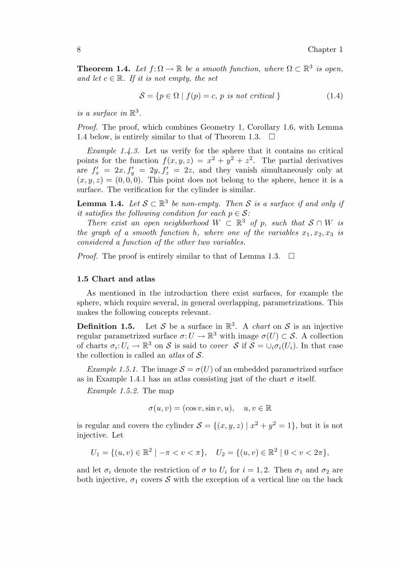
Theorem 1.4. Let f : Ω → R be a smooth function, where Ω ⊂ R3 is open,and let c ∈ R. If it is not empty, the set

S = p ∈ Ω | f(p) = c, p is not critical (1.4)

is a surface in R3.

Proof. The proof, which combines Geometry 1, Corollary 1.6, with Lemma1.4 below, is entirely similar to that of Theorem 1.3.

Example 1.4.3. Let us verify for the sphere that it contains no criticalpoints for the function f(x, y, z) = x2 + y2 + z2. The partial derivativesare f ′

x = 2x, f ′y = 2y, f ′

z = 2z, and they vanish simultaneously only at(x, y, z) = (0, 0, 0). This point does not belong to the sphere, hence it is asurface. The verification for the cylinder is similar.

Lemma 1.4. Let S ⊂ R3 be non-empty. Then S is a surface if and only ifit satisfies the following condition for each p ∈ S:

There exist an open neighborhood W ⊂ R3 of p, such that S ∩ W isthe graph of a smooth function h, where one of the variables x1, x2, x3 isconsidered a function of the other two variables.

Proof. The proof is entirely similar to that of Lemma 1.3.

1.5 Chart and atlas

As mentioned in the introduction there exist surfaces, for example thesphere, which require several, in general overlapping, parametrizations. Thismakes the following concepts relevant.

Definition 1.5. Let S be a surface in R3. A chart on S is an injectiveregular parametrized surface σ:U → R3 with image σ(U) ⊂ S. A collectionof charts σi:Ui → R3 on S is said to cover S if S = ∪iσi(Ui). In that casethe collection is called an atlas of S.

Example 1.5.1. The image S = σ(U) of an embedded parametrized surfaceas in Example 1.4.1 has an atlas consisting just of the chart σ itself.

Example 1.5.2. The map

σ(u, v) = (cos v, sin v, u), u, v ∈ R

is regular and covers the cylinder S = (x, y, z) | x2 + y2 = 1, but it is notinjective. Let

U1 = (u, v) ∈ R2 | −π < v < π, U2 = (u, v) ∈ R2 | 0 < v < 2π,

and let σi denote the restriction of σ to Ui for i = 1, 2. Then σ1 and σ2 areboth injective, σ1 covers S with the exception of a vertical line on the back


where x = −1, and σ2 covers with the exception of a vertical line on the frontwhere x = 1. Together they cover the entire set and thus they constitute anatlas.

y

z

x

Example 1.5.3. The spherical coordinate map

σ(u, v) = (cosu cos v, cosu sin v, sinu), −π2 < u < π

2 , −π < v < π,

and its variation

σ(u, v) = (cosu cos v, sinu, cosu sin v), −π2< u < π

2, 0 < v < 2π,

are charts on the unit sphere. The restrictions on u and v ensure that theyare regular and injective. The chart σ covers the sphere except a half circle(a meridian) in the xz-plane, on the back where x ≤ 0, and the chart σsimilarly covers with the exception of a half circle in the xy-plane, on thefront where x ≥ 0 (half of the ‘equator’). As seen in the following figure theexcepted half-circles are disjoint. Hence the two charts together cover thefull sphere and they constitute an atlas.

y

z

x

Theorem 1.5. Let S be a surface. There exists an atlas of it.

Proof. For each p ∈ S we choose an embedded parametrized surface σ as inDefinition 1.4. Since a homeomorphism is injective, this parametrization isa chart on S. The collection of all these charts is an atlas.

10 Chapter 1

1.6 Manifolds

We now return to the general situation where m and n are arbitraryintegers with 0 ≤ m ≤ n.

Definition 1.6.1. An m-dimensional manifold in Rn is a non-empty setS ⊂ Rn satisfying the following property for each point p ∈ S. There existsan open neighborhood W ⊂ Rn of p and an m-dimensional embedded (seeDefinition 1.2.2) parametrized manifold σ:U → Rn with image σ(U) = S∩W.

The surrounding space Rn is said to be the ambient space of the manifold.

Clearly this generalizes Definitions 1.3 and 1.4, a curve is a 1-dimensionalmanifold in R2 and a surface is a 2-dimensional manifold in R3.

Example 1.6.1 The case m = 0. It was explained in Section 1.1 that a0-dimensional parametrized manifold is a map R0 = 0 → Rn, whose imageconsists of a single point p. An element p in a set S ⊂ Rn is called isolatedif it is the only point from S in some neighborhood of p, and the set S iscalled discrete if all its points are isolated. By going over Definition 1.6.1 forthe case m = 0 it is seen that a 0-dimensional manifold in Rn is the same asa discrete subset.

Example 1.6.2 If we identify Rm with the set (x1, . . . , xm, 0 . . . , 0) ⊂ Rn,it is an m-dimensional manifold in Rn.

Example 1.6.3 An open set Ω ⊂ Rn is an n-dimensional manifold in Rn.Indeed, we can take W = Ω and σ = the identity map in Definition 1.6.1.

Example 1.6.4 Let S′ ⊂ S be a relatively open subset of an m-dimensionalmanifold in Rn. Then S′ is an m-dimensional manifold in Rn.

The following lemma generalizes Lemmas 1.3 and 1.4.

Lemma 1.6. Let S ⊂ Rn be non-empty. Then S is an m-dimensionalmanifold if and only if it satisfies the following condition for each p ∈ S:

There exist an open neighborhood W ⊂ Rn of p, such that S ∩W is thegraph of a smooth function h, where n − m of the variables x1, . . . , xn areconsidered as functions of the remaining m variables.

Proof. The proof is entirely similar to that of Lemma 1.3.

Theorem 1.6. Let f : Ω → Rk be a smooth function, where k ≤ n and whereΩ ⊂ Rn is open, and let c ∈ Rk. If it is not empty, the set

S = p ∈ Ω | f(p) = c, rankDf(p) = k

is an n−k-dimensional manifold in Rn.

Proof. Similar to that of Theorem 1.3 for curves, by means of the implicitfunction theorem (Geometry 1, Corollary 1.6) and Lemma 1.6.


A manifold S in Rn which is constructed as in Theorem 1.6 as the set ofsolutions to an equation f(x) = c is often called a variety. In particular, if theequation is algebraic, which means that the coordinates of f are polynomialsin x1, . . . , xn, then S is called an algebraic variety.

Example 1.6.5 In analogy with Example 1.4.3 we can verify that the m-sphere

Sm = x ∈ Rm+1 | x21 + · · · + x2

m+1 = 1

is an m-dimensional manifold in Rm+1.

Example 1.6.6 The set

S = S1 × S1 = x ∈ R4 | x21 + x2

2 = x23 + x2

4 = 1

is a 2-dimensional manifold in R4. Let

f(x1, x2, x3, x4) =

(

x21 + x2

2

x23 + x2

4

)

,

then

Df(x) =

(

2x1 2x2 0 00 0 2x3 2x4

)

and it is easily seen that this matrix has rank 2 for all x ∈ S.

Definition 1.6.2. Let S be an m-dimensional manifold in Rn. A chart onS is an m-dimensional injective regular parametrized manifold σ:U → Rn

with image σ(U) ⊂ S, and an atlas is a collection of charts σi:Ui → Rn

which cover S, that is, S = ∪iσi(Ui).

As in Theorem 1.5 it is seen that every manifold in Rn possesses an atlas.

1.7 The coordinate map of a chart

In Definition 1.6.2 we require that σ is injective, but we do not requirethat the inverse map is continuous, as in Definition 1.6.1. Surprisingly, itturns out that the inverse map has an even stronger property, it is smoothin a certain sense.

Definition 1.7. Let S be a manifold in Rn, and let σ:U → S be a chart.If p ∈ S we call (x1, . . . , xm) ∈ U the coordinates of p with respect to σ whenp = σ(x). The map σ−1: σ(U) → U is called the coordinate map of σ.

12 Chapter 1

Theorem 1.7. Let σ:U → Rn be a chart on a manifold S ⊂ Rn, and letp0 ∈ σ(U) be given. The coordinate map σ−1 allows a smooth extension,defined on an open neighborhood of p0 in Rn.

More precisely, let q0 ∈ U with p0 = σ(q0). Then there exist open neigh-borhoods W ⊂ Rn of p0 and V ⊂ U of q0 such that

σ(V ) = S ∩W, (1.5)

and a smooth map ϕ:W → V such that

ϕ(σ(q)) = q (1.6)

for all q ∈ V .

Proof. Let W ⊂ Rn be an open neighborhood of p0 in which S is paramet-rized as a graph, as in Lemma 1.6. Say the graph is of the form

σ(x1, . . . , xm) = (x, h(x)) ∈ Rn,

where U ⊂ Rm is open and h: U → Rn−m smooth, then S ∩W = σ(U). Letπ(x1, . . . , xn) = (x1, . . . , xm), then

σ(π(p)) = p

for each point p = (x, h(x)) in S ∩W .

Since σ is continuous, the subset U1 = σ−1(W ) of U is open. The map

π σ:U1 → U is smooth, being composed by smooth maps, and it satisfies

σ (π σ) = σ. (1.7)

By the chain rule for smooth maps we have the matrix product equality

D(σ)D(π σ) = Dσ,

and since the n ×m matrix Dσ on the right has independent columns, thedeterminant of the m×m matrix D(π σ) must be non-zero in each x ∈ U1

(according to the rule from matrix algebra that rank(AB) ≤ rank(B)).

By the inverse function theorem, there exists open sets V ⊂ U1 and V ⊂ Uaround q0 and π(σ(q0)), respectively, such that π σ restricts to a diffeomor-

phism of V onto V . Note that σ(V ) = σ(V ) by (1.7).


U

V

U

V

σ σ π

π σ

S

σ(U)

σ(U)

Let W = W ∩ π−1(V ) ⊂ Rn. This is an open set, and it satisfies

S ∩ W = S ∩W ∩ π−1(V ) = σ(U) ∩ π−1(V ) = σ(V ) = σ(V ).

The map ϕ = (π σ)−1 π: W → V is smooth and satisfies (1.6).

Corollary 1.7. Let σ:U → S be a chart. Then σ is an embedded paramet-rized manifold, and the image σ(U) is relatively open in S.

Proof. For each q0 ∈ U we choose open sets V ⊂ U and W ⊂ Rn, and amap ϕ:W → V as in Theorem 1.7. The inverse of σ is the restriction of thesmooth map ϕ, hence in particular it is continuous. Furthermore, the unionof all these sets W is open and intersects S exactly in σ(U). Hence σ(U) isrelatively open, according to Definition 1.2.3.

It follows from the corollary that every chart on a manifold satisfies thecondition in Definition 1.6.1 of being imbedded with open image. This doesnot render that condition superfluous, however. The point is that once it isknown that S is a manifold, then the condition is automatically fulfilled forall charts on S.

1.8 Transition maps

Since the charts in an atlas of a manifold S in Rn may overlap with eachother, it is important to study the change from one chart to another. Themap σ−1

2 σ1: x 7→ x, which maps a set of coordinates x in a chart σ1 to thecoordinates of the image σ1(x) with respect to another chart σ2, is called

14 Chapter 1

the transition map between the charts. We will show that such a change ofcoordinates is just a reparametrization.

Let Ω ⊂ Rk be open and let f : Ω → Rn be a smooth map with f(Ω) ⊂ S.Let σ:U → Rn be a chart on S, then the map σ−1 f , which is defined on

f−1(σ(U)) = x ∈ Ω | f(x) ∈ σ(U) ⊂ Rk,

is called the coordinate expression for f with respect to σ.

Lemma 1.8. The set f−1(σ(U)) is open and the coordinate expression issmooth from this set into U .

Proof. Since f is continuous into S, and σ(U) is open by Corollary 1.7, itfollows that the inverse image f−1(σ(U)) is open. Furthermore, if an elementx0 in this set is given, we let p0 = f(x0) and choose V , W and ϕ:W → Vas in Theorem 1.7. It follows that σ−1 f = ϕ f in a neighborhood of x0.The latter map is smooth, being composed by smooth maps.

Theorem 1.8. Let S be a manifold in Rn, and let σ1:U1 → Rn and σ2:U2 →Rn be charts on S. Let

Vi = σ−1i (σ1(U1) ∩ σ2(U2)) ⊂ Ui

for i = 1, 2. These are open sets and the transition map

σ−12 σ1:V1 → V2 ⊂ Rm

is a diffeomorphism.

U1 ⊂ Rm

V1

U2 ⊂ Rm

V2

σ1 σ2

σ−12 σ1

S ⊂ Rnσ1(U)

σ2(U)

Proof. Immediate from Lemma 1.8.

Chapter 2

Abstract manifolds

The notion of a manifold S defined in the preceding chapter assumes S tobe a subset of a Euclidean space Rn. However, a more axiomatic and abstractapproach to differential geometry is possible, and in many ways preferable.Of course, a manifold in Rn must satisfy the axioms that we set up for anabstract manifold. Our axioms will be based on properties of charts.

From the point of view of differential geometry the most important prop-erty of a manifold is that it allows the concept of a smooth function. Wewill define this notion and the more general notion of a smooth map betweenabstract manifolds.

2.1 Topological spaces

Since the aim of differential geometry is to bring the methods of differentialcalculus into geometry, the most important property that we wish an abstractmanifold to have is the possibility of differentiating functions on it. However,before we can speak of differentiable functions, we must be able to speak ofcontinuous functions. In this preliminary section we will briefly introduce theabstract framework for that, the structure of a topological space. Topologicalspaces is a topic of general topology, here we will just introduce the mostessential notions. Although the framework is more general, the concepts weintroduce will be familiar to a reader who is acquainted with the theory ofmetric spaces.

Definition 2.1.1. A topological space is a non-empty set X equipped witha distinguished family of subsets, called the open sets, with the followingproperties:

1) the empty set and the set X are both open,2) the intersection of any finite collection of open sets is again open,3) the union of any collection (finite or infinite) of open sets is again open.

Example 2.1.1 In the Euclidean spaces X = Rk there is a standard notionof open sets, and the properties in the above axioms are known to hold. ThusRk is a topological space.

Example 2.1.2 Let X be a metric space. Again there is a standard notionof open sets in X , and it is a fundamental result from the theory of metricspaces that the family of all open sets in X has the properties above. In thisfashion every metric space is a topological space.

16 Chapter 2

Example 2.1.3 Let X be an arbitrary set. If we equipX with the collectionconsisting just of the empty set and X , it becomes a topological space. Wesay in this case that X has the trivial topology. In general this topology doesnot result from a metric, as in Example 2.1.2. The topology on X obtainedfrom the collection of all subsets, is called the discrete topology. It resultsfrom the discrete metric, by which all non-trivial distances are 1.

The following definitions are generalizations of well-known definitions inthe theory of Euclidean spaces, and more generally, metric spaces.

Definition 2.1.2. A neighborhood of a point x ∈ X is a subset U ⊂ Xwith the property that it contains an open set containing x. The interiorof a set A ⊂ X , denoted A, is the set of all points x ∈ A for which A is aneighborhood of x.

Being the union of all the open subsets of A, the interior A is itself anopen set, according to Definition 2.1.1.

Definition 2.1.3. Let A ⊂ X be a subset. It is said to be closed if itscomplement Ac in X is open. In general, the closure of A, denoted A, is theset of all points x ∈ X for which every neighborhood contains a point fromA, and the boundary of A is the set difference ∂A = A \ A, which consistsof all points with the property that each neighborhood meets with both Aand Ac.

It is easily seen that the closure A is the complement of the interior (Ac)

of Ac. Hence it is a closed set. Likewise, the boundary ∂A is closed.

Definition 2.1.4. Let X and Y be topological spaces, and let f :X → Ybe a map. Then f is said to be continuous at a point x ∈ X if for everyneighborhood V of f(x) in Y there exists a neighborhood U of x in X suchthat f(U) ⊂ V , and f is said to be continuous if it is continuous at everyx ∈ X .

Lemma 2.1.1. The map f :X → Y is continuous if and only if the inverseimage of every open set in Y is open in X.

Proof. The proof is straightforward.

Every (non-empty) subset A of a metric space X is in a natural way ametric space of its own, when equipped with the restriction of the distancefunction of X . The open sets in this metric space A are the relatively opensets, that is, the sets A∩W where W is an open subset of X (see Definition1.2.3). This observation has the following generalization.

Lemma 2.1.2. Let X be a topological space, and let A ⊂ X be non-empty.Then A is a topological space of its own, when equipped with the collection ofall subsets of A of the form A ∩O, where O is open in X.

Abstract manifolds 17

Proof. The conditions in Definition 2.1.1 are easily verified.

A subset A of a topological space is always assumed to carry the topologyof Lemma 2.1.2, unless otherwise is mentioned. It is called the induced (orrelative) topology, and the open sets are said to be relatively open.

If A ⊂ X is a subset and f is a map A→ Y , then f is said to be continuousat x ∈ A, if it is continuous with respect to the induced topology. It is easilyseen that if f :X → Y is continuous at x ∈ A, then the restriction f |A:A→ Yis also continuous at x.

Definition 2.1.5. Let X and Y be topological spaces, and let A ⊂ X andB ⊂ Y . A map f :A→ B which is continuous, bijective and has a continuousinverse is called a homeomorphism (compare Definition 1.2.1).

Finally, we mention the following important property of a topologicalspace, which is often assumed in order to exclude some rather peculiar topo-logical spaces.

Definition 2.1.6. A topological space X is said to be Hausdorff if for everypair of distinct points x, y ∈ X there exist disjoint neighborhoods of x and y.

Every metric space is Hausdorff, because if x and y are distinct points,then their mutual distance is positive, and the open balls centered at x andy with radius half of this distance will be disjoint by the triangle inequality.On the other hand, equipped with the trivial topology (see example 2.1.3),a set of at least two elements is not a Hausdorff topological space.

2.2 Abstract manifolds

Let M be a Hausdorff topological space, and let m ≥ 0 be a fixed naturalnumber.

Definition 2.2.1. An m-dimensional smooth atlas of M is a collection(Oi)i∈I of open sets Oi in M such that M = ∪i∈IOi, together with a collec-tion (Ui)i∈I of open sets in Rm and a collection of homeomorphisms, calledcharts, σi:Ui → Oi = σi(Ui), with the following property of smooth transi-tion on overlaps:

For each pair i, j ∈ I the map σ−1j σi is smooth from the open set

σ−1i (Oi ∩Oj) ⊂ Rm to Rm.

Example 2.2 Let S ⊂ Rn be an m-dimensional manifold in Rn (see Defini-tion 1.6.1), which we equip with an atlas as in Definition 1.6.2 (as mentionedbelow the definition, such an atlas exists). It follows from Corollary 1.7 thatfor each chart σ the image O = σ(U) is open in S and σ:U → O is a home-omorphism. Furthermore, it follows from Theorem 1.8 that the transitionmaps are smooth. Hence this atlas on S is a smooth atlas according toDefinition 2.2.1.

18 Chapter 2

In the preceding example S was equipped with an atlas as in Definition1.6.2, but one must keep in mind that there is not a unique atlas associatedwith a given manifold in Rn. For example, the use of spherical coordinates isjust one of many ways to parametrize the sphere. If we use a different atlason S, it is still the same manifold in Rn. In order to treat this phenomenonabstractly, we introduce an equivalence relation for different atlases on thesame space M .

Definition 2.2.2. Two m-dimensional smooth atlases on M are said to becompatible, if every chart from one atlas has smooth transition on its overlapwith every chart from the other atlas (or equivalently, if their union is againan atlas).

It can be seen that compatibility is an equivalence relation. An equiv-alence class of smooth atlases is called a smooth structure. It follows fromTheorem 1.8 that all atlases (Definition 1.6.2) on a given manifold S in Rn

are compatible. The smooth structure so obtained on S is called the standardsmooth structure.

Definition 2.2.3. An abstract manifold (or just a manifold) of dimen-sion m, is a Hausdorff topological space M , equipped with an m-dimensionalsmooth atlas. Compatible atlases are regarded as belonging to the same ma-nifold (the precise definition is thus that a manifold is a Hausdorff topologicalspace equipped with a smooth structure). A chart on M is a chart from anyatlas compatible with the structure.

It is often required of an abstract manifold that it should have a countableatlas (see Section 2.9). We do not require this here.

2.3 Examples

Example 2.3.1 Let M be an m-dimensional real vector space. Fix a basisv1, . . . , vm for M , then the map

σ: (x1, . . . , xm) 7→ x1v1 + · · · + xmvm

is a linear bijection Rm → M . We equip M with the distance functionso that this map is an isometry, then M is a metric space. Furthermore,the collection consisting just of the map σ, is an atlas. Hence M is an m-dimensional abstract manifold.

If another basis w1, . . . , wm is chosen, the atlas consisting of the map

τ : (x1, . . . , xm) 7→ x1w1 + · · · + xmwm

is compatible with the previous atlas. The transition maps σ−1 τ andτ−1 σ are linear, hence smooth. In other words, the smooth structure of Mis independent of the choice of the basis.


Example 2.3.2 This example generalizes Example 1.6.4. Let M be anabstract manifold, and let M ′ be an open subset. For each chart σi:Ui →Oi ⊂M , let O′

i = M ′∩Oi, this is an open subset of M ′, and the collection ofall these sets cover M ′. Furthermore, U ′

i = σ−1i (O′

i) is open in Rm, and therestriction σ′

i of σi to this set is a homeomorphism onto its image. Clearly thetransition maps (σ′

j)−1 σ′

i are smooth, and thus M ′ is an abstract manifoldwith the atlas consisting of all these restricted charts.

Example 2.3.3 Let M = R equipped with the standard metric. Let σ(t) =t3 for t ∈ U = R, then σ is a homeomorphism U → M . The collection ofthis map alone is an atlas on M . The corresponding differential structure onR is different from the standard differential structure, for the transition mapσ−1 i between σ and the identity is not smooth at t = 0.

Example 2.3.4 Let X be an arbitrary set, equipped with the discrete topol-ogy. For each point x ∈ X , we define a map σ: R0 → X by σ(0) = x. Thecollection of all these maps is a 0-dimensional smooth atlas on X .

2.4 Projective space

In this section we give an example of an abstract manifold constructedwithout a surrounding space Rn.

Let M = RPm be the set of 1-dimensional linear subspaces of Rm+1. Itis called real projective space, and can be given the structure of an abstractm-dimensional manifold as follows.

Assume for simplicity that m = 2. Let π: x 7→ [x] = spanx denote thenatural map of R3 \0 onto M , and let S ⊂ R3 denote the unit sphere. Therestriction of π to S is two-to-one, for each p ∈ M there are precisely twoelements ±x ∈ S with π(x) = p. We thus have a model for M as the set ofall pairs of antipodal points in S.

We shall equipM as a Hausdorff topological space as follows. A set A ⊂Mis declared to be open if and only if its preimage π−1(A) is open in R3 (orequivalently, if π−1(A) ∩ S is open in S). We say that M has the quotienttopology relative to R3\0. The conditions for a Hausdorff topological spaceare easily verified. It follows immediately from Lemma 2.1.1 that the mapπ: R3 \ 0 → M is continuous, and that a map f :M → Y is continuous ifand only if f π is continuous.

For i = 1, 2, 3 let Oi denote the subset [x] | xi 6= 0 in M . It is opensince π−1(Oi) = x | xi 6= 0 is open in R3. Let Ui = R2 and let σi:Ui →Mbe the map defined by

σ1(u) = [(1, u1, u2)], σ2(u) = [(u1, 1, u2)], σ3(u) = [(u1, u2, 1)]

for u ∈ R2. It is continuous since it is composed by π and a continuous mapR2 → R3. Moreover, σi is a bijection of Ui onto Oi, and M = O1 ∪O2 ∪O3.

20 Chapter 2

Theorem 2.4.1. The collection of the three maps σi:Ui → Oi forms asmooth atlas on M .

Proof. It remains to check the following.1) σ−1

i is continuous Oi → R2. For example

σ−11 (p) = (

x2

x1,x3

x1)

when p = π[x]. The ratios x2

x1and x3

x1are continuous functions on R3 \ x1 =

0, hence σ−1 π is continuous.2) The overlap between σi and σj satisfies smooth transition. For example

σ−11 σ2(u) = (

1

u1,u2

u1),

which is smooth R2 \ u | u1 = 0 → R2.

2.5 Product manifolds

If M and N are metric spaces, the Cartesian product M × N is again ametric space with the distance function

d((m1, n1), (m2, n2)) = max(dM (m1, m2), dN(n1, n2)).

Likewise, if M and N are Hausdorff topological spaces, then the productM×N is a Hausdorff topological space in a natural fashion with the so-calledproduct topology, in which a subset R ⊂M ×N is open if and only if for eachpoint (p, q) ∈ R there exist open sets P and Q of M and N respectively, suchthat (p, q) ∈ P × Q ⊂ R (the verification that this is a topological space isquite straightforward).

Example 2.5.1 It is sometimes useful to identify Rm+n with Rm × Rn. Inthis identification, the product topology of the standard topologies on Rm

and Rn is the standard topology on Rm+n.

Let M and N be abstract manifolds of dimensions m and n, respectively.For each chart σ:U →M and each chart τ :V → N we define

σ × τ :U × V →M ×N by σ × τ(x, y) = (σ(x), τ(y)).

Theorem 2.5. The collection of the maps σ × τ is an m + n-dimensionalsmooth atlas on M ×N .

Proof. The proof is straightforward.

We call M ×N equipped with the smooth structure given by this atlas forthe product manifold of M and N . The smooth structure on M×N dependsonly on the smooth structures on M and N , not on the chosen atlases.


Notice that if M is a manifold in Rk and N is a manifold in Rl, thenwe can regard M × N as a subset of Rk+l in a natural fashion. It is easilyseen that this subset of Rk+l is an m + n-dimensional manifold (accordingto Definition 1.6.2), and that its differential structure is the same as thatprovided by Theorem 2.5, where the product is regarded as an ‘abstract’ set.

Example 2.5.2 The product S1×R is an ‘abstract’ version of the cylinder.As just remarked, it can be regarded as a subset of R2+1 = R3, and then itbecomes the usual cylinder.

The product S1×S1, which is an ‘abstract’ version of the torus, is naturallyregarded as a manifold in R4. The usual torus, which is a surface in R3, isnot identical with this set, but there is a natural bijective correspondence.

2.6 Smooth maps in Euclidean spaces

We shall now define the important notion of a smooth map between man-ifolds. We first study the case of manifolds in Rn.

Notice that the standard definition of differentiability in a point p of amap f : Rn → Rl requires f to be defined in an open neighborhood of p in Rn.This definition does not make sense for a map defined on an m-dimensionalmanifold in Rn, because in general a manifold is not an open subset of Rn.

Definition 2.6.1. Let X ⊂ Rn and Y ⊂ Rl be arbitrary subsets. A mapf :X → Y is said to be smooth at p ∈ X , if there exists an open set W ⊂ Rn

around p and a smooth map F :W → Rl which coincides with f on W ∩X .The map f is called smooth if it is smooth at every p ∈ X .

If f is a bijection of X onto Y , and if both f and f−1 are smooth, then fis called a diffeomorphism.

A smooth map F as above is called a local smooth extension of f . Inorder to show that a map defined on a subset of Rn is smooth, one thushas to find such a local smooth extension near every point in the domain ofdefinition. It is easily seen that a smooth function is continuous accordingto Definition 2.1.4. We observe that the new notion of smoothness agreeswith the standard definition when X is open in Rn. We also observe thatthe smoothness of f does not depend on which subset of Rl is considered asthe target set Y .

Definition 2.6.2. Let S ⊂ Rn and S ⊂ Rl be manifolds. A map f :S → Sis called smooth if it is smooth according to Definition 2.6.1 with X = S andY = S.

In particular, the above definition can be applied with S = R. A smoothmap f :S → R is said to be a smooth function, and the set of these is denotedC∞(S). It is easily seen that C∞(S) is a vector space when equipped with thestandard addition and scalar multiplication of functions. Since a relativelyopen set Ω ⊂ S is a manifold of its own (see Example 1.6.4), the space C∞(Ω)

22 Chapter 2

is defined for all such sets. It is easily seen that that restriction f 7→ f |Ωmaps C∞(S) → C∞(Ω).

Example 2.6.1 The functions x 7→ xi where i = 1, . . . , n are smooth func-tions on Rn. Hence they restrict to smooth functions on every manifoldS ⊂ Rn.

Example 2.6.2 Let S ⊂ R2 be the circle x | x21 + x2

2 = 1, and letΩ = S \ (−1, 0). The function f : Ω → R defined by f(x1, x2) = x2

1+x1is a

smooth function, since it is the restriction of the smooth function F :W → R

defined by the same expression for x ∈W = x ∈ R2 | x1 6= −1.Example 2.6.3 Let S ⊂ Rn be an m-dimensional manifold, and let σ:U →

S be a chart. It follows from Theorem 1.7 that σ−1 is smooth σ(U) → Rm.

Lemma 2.6. Let X ⊂ Rn and Y ⊂ Rm. If f :X → Rm is smooth and mapsinto Y , and if in addition g:Y → Rl is smooth, then so is g f :X → Rl.

Proof. Let p ∈ X be given, and let F :W → Rm be a local smooth extensionof f around p. Likewise let G:V → Rl be a local smooth extension of garound f(p) ∈ Y . The set W ′ = F−1(V ) is an open neighborhood of p, andG (F |W ′) is a local smooth extension of g f at p.

The definition of smoothness that we have given for manifolds in Rn usesthe ambient space Rn. In order to prepare for the generalization to abstractmanifolds, we shall now give an alternative description.

Theorem 2.6. Let f :S → Rl be a map. If f is smooth, then f σ is smoothfor each chart σ on S. Conversely, if f σ is smooth for each chart in someatlas of S, then f is smooth.

Proof. The first statement is immediate from Lemma 2.6. For the converse,assume f σ is smooth and apply Lemma 2.6 and Example 2.6.3 to f |σ(U) =

(f σ) σ−1. It follows that f |σ(U) is smooth. If this is the case for eachchart in an atlas, then f is smooth around all points p ∈ S.

2.7 Smooth maps between abstract manifolds

Inspired by Theorem 2.6, we can now generalize to abstract manifolds.

Definition 2.7.1. Let M be an abstract manifold of dimension m. A mapf :M → Rl is called smooth if for every chart (σ, U) in a smooth atlas of M ,the map f σ is smooth U → Rl.

The set U is open in Rm, and the smoothness of f σ is in the ordinarysense for functions defined on an open set. It is easily seen that the require-ment in the definition is unchanged if the atlas is replaced by a compatibleone (see Definition 2.2.2), so that the notion only depends on the smoothstructure of M . It follows from Theorem 2.6 that the notion is the same asbefore for manifolds in Rn.


Notice that a smooth map f :M → Rl is continuous, since in a neighbor-hood of each point p ∈M it can be written as (f σ) σ−1 for a chart σ.

Notice also that if Ω ⊂ M is open, then Ω is an abstract manifold of itsown (see Example 2.3.2), and hence it makes sense to speak of smooth mapsf : Ω → Rl. The set of all smooth functions f : Ω → R is denoted C∞(Ω). Itis easily seen that this is a vector space when equipped with the standardaddition and scalar multiplication of functions.

Example 2.7.1 Let σ:U → M be a chart on an abstract manifold M . Itfollows from the assumption of smooth transition on overlaps that σ−1 issmooth σ(U) → Rm.

We have defined what it means for a map from a manifold to be smooth,and we shall now define what smoothness means for a map into a manifold.

As before we begin by considering manifolds in Euclidean space. Let Sand S be manifolds in Rn and Rl, respectively, and let f :S → S. It wasdefined in Definition 2.6.2 what it means for f to be smooth. We will givean alternative description.

Let σ:U → S and σ: U → S be charts on S and S, respectively, whereU ⊂ Rm and U ⊂ Rk are open sets. For a map f :S → S, we call the map

σ−1 f σ: x 7→ σ−1(f(σ(x))), (2.1)

the coordinate expression for f with respect to the charts.The coordinate expression (2.1) is defined for all x ∈ U for which f(σ(x)) ∈

σ(U), that is, it is defined on the set

σ−1(f−1(σ(U))) ⊂ U, (2.2)

and it maps into U .

U ⊂ Rm U ⊂ Rk

S ⊂ Rn S ⊂ Rl

σ σ

σ−1 f σ

f

24 Chapter 2

It follows from Corollary 1.7 that σ(U) is open in S. Hence if f is contin-

uous, then f−1(σ(U)) is open in S by Lemma 2.1.1. Since σ is continuous,the set (2.2), on which σ−1 f σ is defined, is then open.

Theorem 2.7. Let f :S → S be a map. If f is smooth (according to Defi-nition 2.6.2) then it is continuous and σ−1 f σ is smooth, for all charts σ

and σ on S and S, respectively.Conversely, assume that for each p ∈ S there exists a chart σ:U → S

around p, and a chart σ: U → S around f(p), such that f(σ(U)) ⊂ σ(U) andsuch that the coordinate expression σ−1 f σ is smooth, then f is smooth.

Proof. Assume that f is smooth. It was remarked below Definition 2.6.1 thatthen it is continuous. Hence (2.2) is open. It follows from Theorem 2.6 thatf σ is smooth for all charts σ on S. Hence its restriction to the set (2.2)is also smooth, and it follows from Lemma 2.6 and Example 2.6.3 that thecomposed map σ−1 f σ is smooth.

For the converse let p ∈ S be arbitrary and let σ and σ be as stated, suchthat σ−1 f σ is smooth. The identity

f σ = σ (σ−1 f σ),

shows that f σ is smooth. Since the charts σ for all p comprise an atlas forS this implies that f is smooth, according to Theorem 2.6.

By using the formulation of smoothness in Theorem 2.7, we can now gen-eralize the notion. Let M and M be abstract manifolds, and let f :M → Mbe a continuous map. Assume σ:U → σ(U) ⊂M and σ: U → σ(U) ⊂ M arecharts on the two manifolds, then as before

σ−1(f−1(σ(U))) ⊂ U

is an open subset of U , because f is continuous. Again we call the map

σ−1 f σ,

which is defined on this set, the coordinate expression for f with respect tothe given charts.

Definition 2.7.2. Let f :M → M be a map between abstract manifolds.Then f is called smooth if for each p ∈ S there exists a chart σ:U → Maround p, and a chart σ: U → M around f(p), such that f(σ(U)) ⊂ σ(U)and such that the coordinate expression σ−1 f σ is smooth.

A bijective map f :M → M , is called a diffeomorphism if f and f−1 areboth smooth.

Notice that a smooth map M → M is continuous. This follows immedi-ately from the definition above, by writing f = σ (σ−1 f σ) σ−1 in aneighborhood of each point.


Again it should be checked that the notions are independent of the atlasesfrom which the charts are chosen, as long as each atlas is replaced by acompatible one. The verification of this fact is straightforward.

It follows from Theorem 2.7 that the notion of smoothness is the same asbefore if M = S ⊂ Rn and M = S ⊂ Rl. Likewise, there is no conflict withDefinition 2.7.1 in case M = Rl, where in Definition 2.7.2 we can use theidentity map for σ: Rl → Rl.

It is easily seen that the composition of two smooth maps between abstractmanifolds is again smooth.

Example 2.7.2 Let M,N be finite dimensional vector spaces of dimensionm and n, respectively. These are abstract manifolds, according to Example2.3.1. Let f :M → N be a linear map. If we choose a basis for each spaceand define the corresponding charts as in Example 2.3.1, then the coordinateexpression for f is a linear map from Rm to Rn (given by the matrix thatrepresents f), hence smooth. It follows from Definition 2.7.2 that f is smooth.If f is bijective, its inverse is also linear, and hence in that case f is adiffeomorphism.

Example 2.7.3 Let σ:U → M be a chart on an abstract m-dimensionalmanifold M . It follows from the assumption of smooth transition on overlapsthat σ is smooth U →M , if we regard U as an m-dimensional manifold (withthe identity chart). By combining this observation with Example 2.7.1, wesee that σ is a diffeomorphism of U onto its image σ(U) (which is open inM by Definition 2.2.1).

Conversely, every diffeomorphism g of a non-empty open subset V ⊂ Rm

onto an open subset in M is a chart on M . Indeed, by the definition ofa chart given at the end of Section 2.2, this means that g should overlapsmoothly with all charts σ in an atlas of M , that is g−1 σ and σ−1 gshould both be smooth (on the sets where they are defined). This followsfrom the preceding observation about compositions of smooth maps.

2.8 Lie groups

Definition 2.8.1. A Lie group is a group G, which is also a manifold, suchthat the group operations

(x, y) 7→ xy, x 7→ x−1,

are smooth maps from G×G, respectively G, into G.

Example 2.8.1 Every finite dimensional real vector space V is a group,with the addition of vectors as the operation and with neutral element 0.The map (x, y) 7→ x + y is linear V × V → V , hence it is smooth (seeExample 2.7.2). Likewise x 7→ −x is smooth and hence V is a Lie group.

26 Chapter 2

Example 2.8.2 The set R× of non-zero real numbers is a 1-dimensionalLie group, with multiplication as the operation and with neutral element1. Likewise the set C× of non-zero complex numbers is a 2-dimensional Liegroup, with complex multiplication as the operation. The smooth structureis determined by the chart (x1, x2) 7→ x1 + ix2. The product

xy = (x1 + ix2)(y1 + iy2) = x1y1 − x2y2 + i(x1y2 + x2y1)

is a smooth function of the entries, and so is the inverse

x−1 = (x1 + ix2)−1 =

x1 − ix2

x21 + x2

2

.

Example 2.8.3 Let G = SO(2), the group of all 2 × 2 real matrices whichare orthogonal, that is, they satisfy the relation AAt = I, and which havedeterminant 1. The set G is in one-to-one correspondence with the unit circlein R2 by the map

(x1, x2) 7→(

x1 x2

−x2 x1

)

.

If we give G the smooth structure so that this map is a diffeomorphism,then it becomes a 1-dimensional Lie group, called the circle group. Themultiplication of matrices is given by a smooth expression in x1 and x2, andso is the inversion x 7→ x−1, which only amounts to a change of sign on x2.

Example 2.8.4 Let G = GL(n,R), the set of all invertible n× n matrices.It is a group, with matrix multiplication as the operation. It is a manifoldin the following fashion. The set M(n,R) of all real n × n matrices is in

bijective correspondence with Rn2

and is therefore a manifold of dimensionn2. The subset G = A ∈ M(n,R) | detA 6= 0 is an open subset, becausethe determinant function is continuous. Hence G is a manifold.

Furthermore, the matrix multiplication M(n,R) × M(n,R) → M(n,R) isgiven by smooth expressions in the entries (involving products and sums),hence it is a smooth map. It follows that the restriction to G × G is alsosmooth.

Finally, the map x 7→ x−1 is smooth G → G, because according toCramer’s formula the entries of the inverse x−1 are given by rational func-tions in the entries of x (with the determinant in the denominator). It followsthat G = GL(n,R) is a Lie group.

Example 2.8.5 Let G be an arbitrary group, equipped with the discretetopology (see Example 2.3.4). It is a 0-dimensional Lie group.

Theorem 2.8. Let G ⊂ GL(n,R) be a subgroup which is also a manifold in

Rn2

. Then G is a Lie group.


Proof. It has to be shown that the multiplication is smooth G × G → G.According to Definition 2.6.1 we need to find local smooth extensions of themultiplication map and the inversion map. This is provided by Example

2.8.4, since GL(n,R) is open in Rn2

.

Example 2.8.6 The group SL(2,R) of 2× 2-matrices of determinant 1 is a3-dimensional manifold in R4, since Theorem 1.6 can be applied with f equal

to the determinant function det(

a b

c d

)

= ad− bc. Hence it is a Lie group.

2.9 Countable atlas

The definition of an atlas of a smooth manifold leaves no limitation onthe size of the family of charts. Sometimes it is useful that the atlas is nottoo large. In this section we introduce an assumptions of this nature. Inparticular, we shall see that all manifolds in Rn satisfy the assumption.

Recall that a set A is said to be countable if it is finite or in one-to-onecorrespondence with N.

Definition 2.9. An atlas of an abstract manifold M is said to be countableif the set of charts in the atlas is countable.

In a topological space X , a base for the topology is a collection of opensets V with the property that for every point x ∈ X and every neighborhoodU of x there exists a member V in the collection, such that x ∈ V ⊂ U . Forexample, in a metric space the collection of all open balls is a base for thetopology.

Example 2.9 As just mentioned, the collection of all open balls B(y, r) is abase for the topology of Rn. In fact, the subcollection of all balls, for whichthe radius as well as the coordinates of the center are rational, is already abase for the topology. For if x ∈ Rn and a neighborhood U is given, thereexists a rational number r > 0 such that B(x, r) ⊂ U . By density of therationals, there exists a point y ∈ B(x, r/2) with rational coordinates, andby the triangle inequality x ∈ B(y, r/2) ⊂ B(x, r) ⊂ U . We conclude that inRn there is a countable base for the topology. The same is then true for anysubset X ⊂ Rn, since the collection of intersections with X of elements froma base for Rn, is a base for the topology in X .

Lemma 2.9. Let M be an abstract manifold. Then M has a countable atlasif and only if there exists a countable base for the topology.

A topological space, for which there exists a countable base, is said to besecond countable.

Proof. Assume that M has a countable atlas. For each chart σ:U → M inthe atlas there is a countable base for the topology of U , according to theexample above, and since σ is a homeomorphism it carries this to a countable

28 Chapter 2

base for σ(U). The collection of all these sets for all the charts in the atlas,is then a countable base for the topology of M , since a countable union ofcountable sets is again countable.

Assume conversely that there is a countable base (Vk)k∈I for the topology.For each k ∈ I, we select a chart σ:U → M for which Vk ⊂ σ(U), if sucha chart exists. The collection of selected charts is clearly countable. Itcovers M , for if x ∈ M is arbitrary, there exists a chart σ (not necessarilyamong the selected) around x, and there exists a member Vk in the base withx ∈ Vk ⊂ σ(U). This member Vk is contained in a chart, hence also in aselected chart, and hence so is x. Hence the collection of selected charts is acountable atlas.

Corollary 2.9. Let S be a manifold in Rn. There exists a countable atlasfor S.

Proof. According to Example 2.9 there is a countable base for the topol-ogy.

In Example 2.3.4 we introduced a 0-dimensional smooth structure on anarbitrary set X , with the discrete topology. Any basis for the topology mustcontain all singleton sets in X . Hence if the set X is not countable, theredoes not exist any countable atlas for this manifold.

2.10 Whitney’s theorem

The following is a famous theorem, due to Whitney. The proof is toodifficult to be given here. In Section 5.6 we shall prove a weaker version ofthe theorem.

Theorem 2.10. Let M be an abstract smooth manifold of dimension m,and assume there exists a countable atlas for M . Then there exists a diffeo-morphism of M onto a manifold in R2m.

For example, the projective space RP2 is diffeomorphic with a 2-dimensio-nal manifold in R4. Notice that the assumption of a countable atlas cannotbe avoided, due to to Corollary 2.9.

The theorem could give one the impression that if we limit our interestto manifolds with a countable atlas, then the notion of abstract manifoldsis superfluous. This is not so, because in many circumstances it would bevery inconvenient to be forced to perceive a particular smooth manifold as asubset of some high-dimensional Rk. The abstract notion frees us from thislimitation.

Chapter 3

The tangent space

In this chapter the tangent space for an abstract manifold is defined.Let us recall from Geometry 1 that for a parametrized surface σ:U → R3

we defined the tangent space at point x ∈ U as the linear subspace in R3

spanned by the derived vectors σ′u and σ′

v at x. The generalization to Rn

is straightforward, it is given below. In this chapter we shall generalize theconcept to abstract manifolds. We shall do so in two steps. The first step isto consider manifolds in Rn. Here we can still define the tangent space withreference to the ambient space Rn. For the abstract manifolds, treated inthe second step, we need to give an abstract definition.

3.1 The tangent space of a parametrized manifold

Let σ:U → Rn be a parametrized manifold, where U ⊂ Rm is open.

Definition 3.1. The tangent space Tx0σ of σ at x0 ∈ U is the linear subspace

of Rn spanned by the columns of the n×m matrix Dσ(x0).

Assume that σ is regular at x0. Then the the columns of Dσ(x0) arelinearly independent, and they form a basis for the space Tx0

σ. If v ∈ Rm

then Dσ(x0)v is the linear combination of these columns with the coordinatesof v as coefficients, hence v 7→ Dσ(x0)v is a linear isomorphism of Rm ontothe m-dimensional tangent space Tx0

σ.Observe that the tangent space is a ‘local’ object, in the sense that if

two parametrized manifolds σ:U → Rn and σ′:U ′ → Rn are equal on someneighborhood of a point x0 ∈ U ∩ U ′, then Tx0

σ = Tx0σ′.

From Geometry 1 we recall the following result, which is easily generalizedto the present setting.

Theorem 3.1. The tangent space is invariant under reparametrization. Inother words, if φ:W → U is a diffeomorphism of open sets in Rm and τ =σ φ, then Ty0

τ = Tφ(y0)σ for all y0 ∈W .

Proof. The proof is essentially the same as in Geometry 1, Theorem 2.7. Bythe chain rule, we have the matrix identity

Dτ(y0) = Dσ(φ(y0))Dφ(y0),

which implies that the columns of Dτ(y0) are linear combinations of thecolumns of Dσ(φ(y0)), hence Ty0

τ ⊂ Tφ(y0)σ. The opposite inclusion followsby the same argument with φ replaced by its inverse.

30 Chapter 3

3.2 The tangent space of a manifold in Rn

Let S ⊂ Rn be a manifold (see Definition 1.6.1).

Definition 3.2. The tangent space of σ at a point p ∈ S is them-dimensionallinear space

TpS = Tx0σ ⊂ Rn, (3.1)

where σ:U → S is an arbitrary chart on S with p = σ(x0) for some x0 ∈ U .

Notice that it follows from Theorem 3.1 that the tangent space TpS = Tx0σ

is actually independent of the chart σ, since any other chart around p willbe a reparametrization, according to Theorem 1.8 (more precisely, it is therestriction to the overlap of the two charts, which is a reparametrization).Notice also the change of notation, in that the footpoint p of TpS belongs toS ⊂ Rn in contrast to the previous footpoint x0 ∈ Rm of Tx0

σ.With the generalization to abstract manifolds in mind we shall give a

different characterization of the tangent space TpS, which is also closelyrelated to a property from Geometry 1 (Theorem 2.4).

We call a parametrized smooth curve γ: I → Rn a parametrized curve onS if the image γ(I) is contained in S.

Theorem 3.2. Let p ∈ S. The tangent space TpS is the set of all vectors inRn, which are tangent vectors γ′(t0) to a parametrized curve on S, γ: I → S,with γ(t0) = p for some t0 ∈ I.

Proof. Let σ:U → S be a chart with p = σ(x0) for some x0 ∈ U . Bydefinition TpS = Tx0

σ. As remarked below Definition 3.1, the map v 7→Dσ(x0)v is a linear isomorphism of Rm onto Tx0

σ. For each v ∈ Rm wedefine a parametrized curve on S by

γv(t) = σ(x0 + tv)

for t close to 0 (so that x0 + tv ∈ U). It then follows from the chain rule that

γv′(0) = Dσ(x0)v,

so we conclude that the map

Tσ: Rm → TpS, v 7→ γv′(0) (3.2)

is a linear isomorphism. In particular, we see that every vector in TpS is atangent vector of a parametrized curve on S.

Conversely, given a parametrized curve γ: I → Rn on S with γ(t0) = p, wedefine a parametrized curve µ in Rm by µ = σ−1 γ for t in a neighborhoodof t0. This is the coordinate expression for γ with respect to σ. It follows

The tangent space 31

from Lemma 1.8 that µ is smooth, and since γ = σ µ, it follows from thechain rule that

γ′(t0) = Dσ(x0)µ′(t0) ∈ Tx0

σ.

This proves the opposite inclusion.

We have described the tangent space as a space of tangent vectors to curveson S. However, it should be emphasized that the correspondence betweencurves and tangent vectors is not one-to-one. In general many different curvesgive rise to the same tangent vector in Rn.

Example 3.2.1 Let Ω ⊂ Rn be an open subset, then Ω is an n-dimensionalmanifold in Rn, with the identity map as a chart (see Example 1.6.3). Thetangent space is Rn, and the map (3.2) is the identity map, since the deriv-ative of t 7→ x0 + tv at t = 0 is v.

Example 3.2.2 Suppose S ⊂ Rn is the n − k-dimensional manifold givenby an equation f(p) = c as in Theorem 1.6, where in addition it is requiredthat Df(p) has rank k for all p ∈ S. Then we claim that the tangent spaceTpS is the null space for the matrix Df(p), that is,

TpS = v ∈ Rn | Df(p)v = 0.

Here we recall that by a fundamental theorem of linear algebra, the dimensionof the null space is n− k when the rank of Df(p) is k.

The claim can be established as follows by means of Theorem 3.2. If vis a tangent vector, then v = γ′(t0) for some parametrized curve on S withp = γ(t0). Since γ maps into S, the function f γ is constant (with the valuec), hence (f γ)′(t0) = 0. It follows from the chain rule that Df(p)v = 0.Thus the tangent space is contained in the null space. Since both are linearspaces of dimension n− k, they must be equal.

Example 3.2.3 Let C denote the ∞-shaped set in Examples 1.2.2 and 1.3.5.The parametrized curve γ(t) = (cos t, cos t sin t) is a parametrized curve onC, and it passes through (0, 0) for each t = k π

2 with k an odd integer. If C was

a curve in R2, then γ′(k π2) would belong to T(0,0)C, according to Theorem

3.2. But the vectors γ′(π2 ) = (−1,−1) and γ′(3π

2 ) = (1,−1) are linearlyindependent, and hence T(0,0)C cannot be a 1-dimensional linear space. Thuswe reach a contradiction, and we conclude that C is not a curve (as mentionedin Example 1.3.5).

3.3 The abstract tangent space

Consider an abstract m-dimensional manifold M , and let σ:U →M be achart. It does not make sense to repeat Definition 3.1 of the tangent spaceto σ, because the n×m-matrix Dσ(x0) is not defined (there is no n). Henceit does not make sense to repeat Definition 3.2 either. Instead, Theorem 3.2will be our inspiration for the definition of the tangent space TpM .

32 Chapter 3

We define a parametrized curve on M to be a smooth map γ: I → M ,where I ⊂ R is open. By definition (see Definition 2.7.2), this means thatσ−1 γ is smooth for all charts on M . As before, if σ is a chart on M , wecall µ = σ−1 γ the coordinate expression of γ with respect to σ. If p ∈ Mis a point, a parametrized curve on M through p, is a parametrized curve onM together with a point t0 ∈ I for which p = γ(t0).

Let γ1: I1 → M and γ2: I2 → M be parametrized curves on M withp = γ1(t1) = γ2(t2), and let σ be a chart around p, say p = σ(x). We saythat γ1 and γ2 are tangential at p, if the coordinate expressions satisfy

(σ−1 γ1)′(t1) = (σ−1 γ2)

′(t2). (3.3)

Lemma 3.3.1. Being tangential at p is an equivalence relation on curvesthrough p. It is independent of the chosen chart σ.

Proof. The first statement is easily seen. If σ is another chart then thecoordinate expressions are related by

σ−1 γi = (σ−1 σ) (σ−1 γi)

on the overlap. The chain rule implies

(σ−1 γi)′(ti) = D(σ−1 σ)(x) (σ−1 γi)

′(ti)

for each of the curves. Hence the relation (3.3) implies the similar relationwith σ replaced by σ.

We write the equivalence relation as γ1 ∼p γ2, and we interprete it as anabstract equality between the ‘tangent vectors’ of the two curves at p. Inspite of the fact that we have not yet defined the tangent vector of a curve onM , we have thus accomplished to make sense out of the statement that thattwo curves have the same tangent vector. This is exactly what is needed inorder to give an abstract version of Definition 3.2.

Definition 3.3. The tangent space TpM is the set of ∼p-classes of parame-trized curves on M through p.

The following observation is of importance, because it shows that theabstract tangent space is a ‘local’ object, that is, it only depends on thestructure of M in a vicinity of p. If M ′ ⊂ M is an open subset, then M ′

is an abstract manifold in itself, according to Example 2.3.2. Obviously aparametrized curve on M ′ can also be regarded as a parametrized curveon M , and the notion of two curves being tangential at a point p ∈ M ′ isindependent of how we regard the curves. It follows that there is a naturalinclusion of TpM

′ in TpM . Conversely, a parametrized curve γ: I → Mthrough p is tangential at p to its own restriction γ|I′ where I ′ = γ−1(M ′),


and the latter is also a parametrized curve on M ′. It follows that TpM′ =

TpM .We need to convince ourselves that the abstractly defined tangent space

agrees with the tangent space of Definition 3.2 in case M = S ⊂ Rn. This isthe content of the following lemma.

Lemma 3.3.2. Let S be a manifold in Rn and let γ1, γ2 be curves on Sthrough p. Then γ1 ∼p γ2 if and only if γ′1(t1) = γ′2(t2).

It follows that the map γ 7→ γ′(t0) induces a bijective map from ∼p-classesof parametrized curves onto the tangent space TpS of Definition 3.2. Hencethe abstract tangent space is in bijective correspondence with the old one.

Proof. Choose a chart σ around p, and let µi = σ−1 γi be the coordinateexpression for γi. Then by definition γ1 ∼p γ2 means that µ′

1(t1) = µ′2(t2).

By applying the chain rule to the expressions γi = σ µi and µi = σ−1 γi

we see that µ′1(t1) = µ′

2(t2) if and only if γ′1(t1) = γ′2(t2). We have usedTheorem 1.7 in order to be able to differentiate σ−1.

3.4 The vector space structure

The definition we have given of TpM has some disadvantages. In particu-lar, it is not clear at all how to organize TpM as a linear space. The elementsof TpM are classes of curves, and they are not easily seen as tangent vec-tors for any reasonable vector space structure. Thus it is in fact prematureto denote TpM a ‘space’. We will remedy this by exhibiting an alternativedescription of TpM , analogous to (3.2).

Theorem 3.4. Let σ:U →M be a chart on M with p = σ(x0).(i) For each element v ∈ Rm let γv(t) = σ(x0 + tv) for t close to 0. The

mapTσ: v 7→ [γv]p

is a bijection of Rm onto TpM . The inverse map is given by

[γ]p 7→ (σ−1 γ)′(t0),

for each curve γ on M with γ(t0) = p.(ii) There exists a unique structure on TpM as a (necessarily m-dimen-

sional) vector space such that the map Tσ is a linear isomorphism. Thisstructure is independent of the chosen chart σ around p.

Proof. (i) Notice that σ−1 γv(t) = x0 + tv, and hence (σ−1 γv)′(0) = v. It

follows that if γv1∼p γv2

then v1 = v2. Hence Tσ is injective. To see that itis surjective, let an element [γ]p ∈ TpM be given, with representative γ suchthat γ(t0) = p. Let σ−1 γ be the coordinate expression of γ with respect

34 Chapter 3

to σ, and put v = (σ−1 γ)′(t0). Then γv ∼p γ because (σ−1 γv)′(0) =

(σ−1 γ)′(t0) = v. Hence Tσ(v) = [γ]p, and the map is surjective.(ii) By means of the bijection Tσ: v 7→ [γv]p we can equip TpM as an m-

dimensional vector space. We simply impose the structure on TpM so thatthis map is an isomorphism, that is, we define addition and scalar multi-plication by the requirement that aTσ(v) + bT σ(w) = Tσ(av + bw) for allv, w ∈ Rm and a, b ∈ R.

Only the independency of σ remains to be seen. Suppose that σ is anotherchart on M around p. We will prove that

Tσ(v) = T σ(D(σ−1 σ)(x0)v) (3.4)

for all v ∈ Rm. Let γ(t) = γv(t) = σ(x0 + tv). By the chain rule

(σ−1 γ)′(0) =d

dt(σ−1 σ)(x0 + tv)|t=0 = D(σ−1 σ)(x0)v.

Applying the last statement of (i), for the chart σ, we conclude that

[γ]p = T σ((σ−1 γ)′(0)) = T σ(D(σ−1 σ)(x0)v),

from which (3.4) follows.Since multiplication by D(σ−1 σ)(x0) is a linear isomorphism of Rm, it

follows from (3.4) that T σ is a linear map if and only if T σ is a linear map.Hence the two bijections induce the same linear structure on TpM .

This theorem is helpful for our understanding of the tangent space. Basedon it we can visualize the tangent space TpM as a ‘copy’ of Rm which isattached to M with its base point at p.

We have introduced a linear structure on TpM , but if M happens to be amanifold S ⊂ Rn then TpS already has such a structure, inherited from theambient Rn. In fact, it follows from the proof of Theorem 3.2, see (3.2), thatthe two structures agree in this case.

Example 3.4.1 Let V be an m-dimensional real vector space regarded as anabstract manifold as in Example 2.3.1. We will show that for each elementp ∈ V there exists a natural isomorphism L:V → TpV . For each vectorr ∈ V we define L(r) to be the ∼p-class of the line p + tr with direction r,regarded as a curve through p. In order to prove that L is an isomorphism ofvector spaces, we choose a basis v1, . . . , vm for V , and let σ: Rm → V denotethe corresponding isomorphism (x1, . . . , xm) 7→ x1v1 + · · · + xmvm, whichconstitutes a chart on V (see Example 2.3.1). For x ∈ Rm and r = σ(x) wehave, with the notation of Theorem 3.4,

p+ tr = p+ tσ(x) = σ(x0 + tx) = γx(t)

and hence Tσ(x) = [γx]p = L(r). Since Tσ is an isomorphism of vectorspaces Rm → TpV , and since x 7→ r = σ(x) is an isomorphism Rm → V , weconclude that r 7→ L(r) is an isomorphism V → TpV .


3.5 Directional derivatives

An important property of tangent vectors is that they can be brought toact on smooth functions as a kind of differentiation operators.

We recall the following concept from multivariable calculus. For a functionf : Ω → R on an open set Ω ⊂ Rn, which is differentiable at a point p ∈ Ω,we define the directional derivative in direction X ∈ Rn as the derivative at0 of the function t 7→ f(p + tX), that is, we differentiate f along the linethrough p with direction X . We denote the directional derivative as follows:

DX(f) =d

dt

∣

∣

∣

t=0f(p+ tX). (3.5)

The directional derivatives in the directions of the canonical basis vectorse1, . . . , en are the partial derivatives

Dei=

∂f

∂xi(p)

and the general directional derivative is related to these partial derivativesthrough the formula

DX(f) =n

∑

i=1

ai∂f

∂xi(p), (3.6)

when X = (a1, . . . , an). In particular, we see that DX(f) depends linearlyon X .

We shall now extend this concept to manifolds in Rn. Let S ⊂ Rn bea manifold and p ∈ S a point. Recall from Definition 2.6.1 that a functionf :S → R is called smooth at p if it has a local smooth extension F :W → R

in a neighborhood W ⊂ Rn of p.

Lemma 3.5. Let f :S → R be smooth at p, and let F :W → R be a localsmooth extension. Let X ∈ TpS be a tangent vector, and let γ: I → S be aparametrized curve on S with γ(t0) = p and γ′(t0) = X. Then

(f γ)′(t0) = DXF. (3.7)

Proof. Since γ maps into S we have f γ = F γ in a neighborhood of t0, andit follows from the chain rule that (F γ)′(t0) = DF (p)γ′(t0), where DF (p)is the 1 × n Jacobian matrix of F at p. Since γ′(t0) = X = (X1, . . . , Xn) wethus obtain

(f γ)′(t0) =n

∑

i=1

∂F

∂xi(p)Xi, (3.8)

and this is exactly DXF according to (3.6) above.

36 Chapter 3

Observe that the left side of (3.7) is independent of the choice of localsmooth extension F of f , and the other side of is independent of the choiceof curve γ with γ′(t0) = X . We conclude that both sides only depend on fand X , so that the following definition is valid.

Definition 3.5. The directional derivative of f at p in direction X ∈ TpSis

DX(f) = (f γ)′(t0),

where γ is chosen as above.

Notice that a tangent vector X ∈ TpS is uniquely determined through itsaction DX on smooth functions. For each i = 1, . . . , n we can determine thei-th coordinate of X by letting it act on the function f(x) = xi (see Example2.6.1), since it follows from (3.8) that DXf = Xi for this function. For thisreason it is quite common to identify X with the operator DX and simplywrite Xf in place of DXf .

Example 3.5 Let S be the unit sphere in R3, let p = (0, 0, 1) ∈ S andlet X ∈ TpS denote the tangent vector X = (1, 3, 0). Consider the functionf(x, y, z) = xz on S. The directional derivative is

DXf = [∂

∂x+ 3

∂

∂y](xz)(p) = 1.

This follows from Lemma 3.5, since F (x, y, z) = xz, (x, y, z) ∈ R3, is asmooth extension of f .

3.6 Action on functions

We have seen in the preceding section that for a manifold in Rn, wecan bring its tangent vectors to act on smooth functions as a differentiationoperator. The same can be done in the abstract case. Let M be an abstractmanifold and let p ∈M .

Lemma 3.6.1. Let γ1, γ2 be parametrized curves on M with p = γ1(t1) =γ2(t2). If γ1 ∼p γ2 then (f γ1)

′(t1) = (f γ2)′(t2) for all f ∈ C∞(M).

Proof. Fix a chart σ:U → M around p, say with p = σ(x0). The composedmap f γi can be written as follows in a neighborhood of ti,

f γi = (f σ) (σ−1 γi).

Applying the chain rule we obtain

(f γi)′(ti) = D(f σ)(x0)(σ

−1 γi)′(ti),

where D(f σ)(x0) is the Jacobian 1×m-matrix of f σ at x0. The lemmafollows immediately from this expression and (3.3).


It is a consequence of this lemma that the following definition is valid (itis independent of the choice of the representative γ).

Definition 3.6. Let X ∈ TpM . The directional derivative in direction Xof a function f ∈ C∞(M) is

DX(f) = (f γ)′(t0),

where γ is any representative of X .

Notice that the action of DX is local, in the sense that if two functionsf1, f2 are equal in a neighborhood of p, then DX(f1) = DX(f2). Notice also,that DXf makes sense also for f ∈ C∞(Ω), when p ∈ Ω ⊂ M with Ω open(use the observation below Definition 3.3).

3.7 The differential of a smooth map

Let M , N be abstract manifolds of dimension m and n, respectively, andlet p ∈ M . Let f :M → N be smooth. The differential, also called tangentmap, of f at p will now be defined. We shall define it as a linear map fromTpM to Tf(p)N . It serves as a generalization of the Jacobian matrix Df(p)of a map f : Rm → Rn (which, in turn, generalizes the ordinary derivative f ′

of f : R → R).If M and N are open subsets of Rm and Rn, then by definition the differ-

ential dfp is the linear map Rm → Rn which has the Jacobian Df(p) as itsmatrix with respect to the standard basis vectors. It satisfies

f(p+ h) − f(p) = dfp(h) + o(h),

which means that|f(p+ h) − f(p) − dfp(h)|

|h| → 0

as h→ 0. The interpretation is that the linear map dfp is an approximationto the increment of f at p.

Notice that if m = 1 and M ⊂ R, then the linear map dfp: R → Rn iscompletely determined by its value dfp(1) ∈ Rn. This value is exactly thederivative f ′(p) ∈ Rn, which constitutes the 1× n-matrix Df(p). This is forexample the case when f = γ is a curve in N .

The important chain rule is valid for the differential of a composed mapf g, where g:L → M and f :M → N are smooth maps between open setsL ⊂ Rl, M ⊂ Rm and N ⊂ Rn. It reads

d(f g)p = dfg(p) dgp,

and it is an immediate consequence of the corresponding chain rule for theJacobians.

38 Chapter 3

Assume that S and T are manifolds in Rk and Rl, respectively, and letf :S → T be smooth. Recall (see Definition 2.6.1) that f has a local smoothextension F :W → Rl in a neighborhood of each point p ∈ S.

Definition 3.7.1. We define the differential

dfp:TpS → Tf(p)T

as the linear map, which is the restriction to the tangent space TpS ⊂ Rk ofthe differential dFp: R

k → Rl of a local smooth extension F of f at p.

It follows from the chain rule, applied to F γ, that

dfp(γ′(t0)) = dFp(dγt0(1)) = d(F γ)t0(1) = (f γ)′(t0) (3.9)

for any smooth curve γ on S with γ(t0) = p. The expression (3.9) shows thatdfp is independent of the choice of the local smooth extension F , and it alsoimplies that dfp maps into Tf(p)N .

Example 3.7.1 Let f :S → R be a smooth function on S. The tangentspace TyR of R at any point y ∈ R is identified with R (see Example 3.2.1).The differential dfp is therefore a linear map TpS → R. It is determined fromthe expression (3.9).

Assume now that M and N are arbitrary abstract manifolds, and letagain f :M → N be smooth. Recall that [γ]p denotes the ∼p-class of γ. Thefollowing definition is inspired by (3.9).

Definition 3.7.2. The differential of f is the map dfp:TpM → Tf(p)Ndefined by

dfp([γ]p) = [f γ]f(p)

for all smooth curves γ on M through p.

Notice that f γ is a smooth curve on N , and [f γ]f(p) is its equivalenceclass in Tf(p)N . In fact, in order for dfp([γ]p) to be well defined, we need toshow that [f γ]f(p) is independent of the choice of representative γ for theclass [γ]p. This is done in the lemma below. Notice also that if M and Nare manifolds in Rk and Rl, then it follows from (3.9) that the differentialsdefined in Definitions 3.7.1 and 3.7.2 agree with each other.

Lemma 3.7.1. Let γ1 and γ2 be smooth curves on M with γ1(t1) = γ2(t2) =p, then

γ1 ∼p γ2 ⇒ f γ1 ∼f(p) f γ2.

Proof. Let τ be a chart on N around f(p), and let σ be a chart on M aroundp. Then for each curve on M through p,

(τ−1 f γ)′(t0) = (τ−1 f σ σ−1 γ)′(t0)

= D(τ−1 f σ)(x0)(σ−1 γ)′(t0) (3.10)


by the chain rule (where x0 is determined by σ(x0) = p). Applying this toγ1 and γ2, the implication of the lemma follows from the definition of theequivalence relations ∼p and ∼f(p).

The chain rule is an easy consequence of Definition 3.7.2. If g:L → Mand f :M → N are smooth maps between abstract manifolds, then

d(f g)p = dfg(p) dgp. (3.11)

Example 3.7.2 We have seen in Example 2.7.3 that a chart σ is a smoothmap U →M . We will determine its differential dσx0

, which is a smooth mapfrom Rm (the tangent space of U at x0) to TpM . Let v ∈ Rm. Then v is thetangent vector at 0 to the curve x0 +tv in U , and hence by definition dσx0

(v)is the tangent vector at 0 to the curve σ(x0 + tv). This curve is exactly thecurve γv, and hence dσx0

(v) = [γv]p. We conclude that the differential dσx0

is exactly the isomorphism Tσ: v 7→ γ′v(0) of Theorem 3.4.

In particular, we conclude from the preceding example that the standardbasis vectors (see Section 3.6) for TpM with respect to σ are the vectors givenby dσx0

(ei) for i = 1, . . . , m, where p = σ(x0).

Theorem 3.7. The differential dfp:TpM → Tf(p)N is a linear map.

Proof. Let a chart σ on M with p = σ(x0) and a chart τ on N with f(p) =τ(y0) be chosen. It follows from the chain rule (3.11) and Example 3.7.2 thatthe following diagram commutes

dσx0

TpMdfp−−−−→ Tf(p)N

x

x

dτy0

Rmd(τ−1fσ)x0−−−−−−−−−→ Rn

where the vertical maps are the isomorphisms of Theorem 3.4 for M and N(see Example 3.7.2). Since the map in the bottom of this diagram is linear,we conclude that dfp:TpM → Tf(p)N is a linear map.

The differential of the identity mapM →M is the identity map id:TpM →TpM . Hence it follows from the chain rule that if f :M → N is a diffeomor-phism, then

d(f−1)f(p) dfp = d(f−1 f)p = id .

From this relation and the similar one with opposite order of f and f−1, wesee that when f is a diffeomorphism, then dfp is bijective with (dfp)

−1 =d(f−1)f(p). We thus obtain that the differential of a diffeomorphism is alinear isomorphism between tangent spaces. In particular, two manifoldsbetween which there exists a diffeomorphism, must have the same dimension.

40 Chapter 3

Notice that the diagram above implies that the matrix for dfp, with re-spect to the standard bases for TpM and Tf(p)N for the given charts, is the

Jacobian D(τ−1 f σ)(x0).

Example 3.7.3 Let f :V → W be a linear map between finite dimensionalvector spaces, as in Example 2.7.2. In Example 3.4.1 we have identifiedthe tangent space TpV of a vector space V with V itself. By applying thisidentification for both V and W , we shall see that the differential at p ∈ Vof a linear map f :V → W is the map f itself. An element v ∈ V = TpV isthe tangent vector to the curve t 7→ p + tv at t = 0. This curve is mappedto t 7→ f(p+ tv) = f(p) + tf(v) by f , and the tangent vector at t = 0 of thelatter curve on W is exactly f(v). Hence dfp(v) = f(v) as claimed.

In Section 3.6 an action of tangent vectors by directional derivations wasdefined. We will now determine the differential in this picture.

Lemma 3.7.2. Let X ∈ TpM and let f :M → N be smooth. Then

Ddfp(X)(ϕ) = DX(ϕ f)

for all ϕ ∈ C∞(N).

Proof. Let γ be a representative of X . Then f γ is a representative ofdfp(X) and hence by Definition 3.6

Ddfp(X)(ϕ) = (ϕ f γ)′(t0) = DX(ϕ f).

3.8 The standard basis

Let M be an abstract manifold. Given a chart σ with p = σ(x0), we obtaina basis for TpM from Theorem 3.4, by taking the isomorphic image T σ(ei) ofeach of the standard basis vectors e1, . . . , em for Rm (in that order), that is,the basis vectors will be the equivalence classes of the curves t 7→ σ(x0 + tei).This basis for TpM is called the standard basis with respect to σ. With thenotation from the preceding section, see Example 3.7.2, the standard basisvectors are

dσx0(e1), . . . , dσx0

(em).

These basis vectors, which depend on the chosen chart σ, can be seen asabstract analogs of the basis vectors

σ′x1, σ′

x2

for the tangent space of a parametrized surface in R3 (the columns of theJacobian Dσ(x0)).


The standard basis vectors determine the following operators D1, . . . ,Dm

of directional differentiation. Let Di = DXiwhere Xi = dσx0

(ei). Then byDefinition 3.6

Dif =d

dt|t=0 f(σ(x0 + tei)) =

∂

∂xi(f σ)(x0). (3.12)

Because of (3.12) it is customary to denote Di by ∂∂xi

.

3.9 Orientation

Let V be a finite dimensional vector space. Two ordered bases (v1, . . . , vn)and (v1, . . . , vn) are said to be equally oriented if the transition matrix S,whose columns are the coordinates of the vectors v1, . . . , vn with respectto the basis (v1, . . . , vn), has positive determinant. Being equally orientedis an equivalence relation among bases, for which there are precisely twoequivalence classes. The space V is said to be oriented if a specific class hasbeen chosen, this class is then called the orientation of V , and its memberbases are called positive. The Euclidean spaces Rn are usually oriented by theclass containing the standard basis (e1, . . . , en). For the null space V = 0we introduce the convention that an orientation is a choice between the signs+ and −.

Example 3.9.1 For a two-dimensional subspace V of R3 it is customaryto assign an orientation by choosing a normal vector N . The positive bases(v1, v2) for V are those for which (v1, v2, N) is a positive basis for R3 (inother words, it is a right-handed triple).

Let σ be a chart on an abstract manifold M , then the tangent space isequipped with the standard basis (see Section 3.6) with respect to σ. Foreach p ∈ σ(U) we say that the orientation of TpM , for which the standardbasis is positive, is the orientation induced by σ.

Definition 3.9. An orientation of an abstract manifold M is an orientationof each tangent space TpM , p ∈ M , such that there exists an atlas of M inwhich all charts induce the given orientation on each tangent space.

The manifold is called orientable if there exists an orientation. If an ori-entation has been chosen we say that M is an oriented manifold and we calla chart positive if it induces the proper orientation on each tangent space.

A diffeomorphism map f :M → N between oriented manifolds of equal di-mension is said to be orientation preserving if for each p ∈M , the differentialdfp maps positive bases for TpM to positive bases for Tf(p)N .

Example 3.9.2 Every manifold M , of which there exists an atlas with onlyone chart, is orientable. The orientation induced by that chart is of coursean orientation of M .

42 Chapter 3

Example 3.9.3 Suppose S ⊂ Rn is the n − k-dimensional manifold givenby an equation f(p) = c as in Theorem 1.6. As seen in Example 3.2.2 thetangent space at p ∈ S is the null space

TpS = X ∈ Rn | Df(p)X = 0.

for the k × n matrix Df(p). Let w1, . . . , wk ∈ Rn denote the rows of Df(p),in the same order as they appear in the matrix. We can then define anorientation of TpS by declaring an ordered basis (v1, . . . , vn−k) positive if thecombined basis (v1, . . . , vn−k, w1, . . . , wk) for Rn is positive with respect tothe standard order. It can be shown that this is an orientation of S, whichis thus orientable.

For a surface in R3 given by f(x) = c, where f is a scalar valued function,this means that we define the orientation by means of the normal given bythe gradient vector w = (∂f

∂x, ∂f

∂y, ∂f

∂z) of f .

Not all manifolds are orientable however, the most famous example beingthe two-dimensional Mobius band. A model for it in R3 can be made bygluing together the ends of a strip which has been given a half twist. It isimpossible to make a consistent choice of orientations, because the band is‘one-sided. Choosing an orientation in one point forces it by continuity tobe given in neighboring points, etcetera, and eventually we are forced to theopposite choice in the initial point.

Chapter 4

Submanifolds

The notion of a submanifold of an abstract smooth manifold will now bedefined. In fact, there exist two different notions of submanifolds, ‘embed-ded submanifolds’ and ‘immersed submanifolds’. Here we shall focus on thestronger notion of embedded submanifolds, and for simplicity we will justuse the term ‘submanifold’.

4.1 Submanifolds in Rk

Definition 4.1. Let S be a manifold in Rk. A submanifold of S is a subsetT ⊂ S, which is also a manifold in Rk.

Lemma 4.1. Let T be a submanifold of S ⊂ Rk. Then dimT ≤ dimS andTpT ⊂ TpS for all p ∈ T . Moreover, the inclusion map i: T → S is smooth,and its differential dip at p ∈ T is the inclusion map TpT → TpS.

Proof. By Theorem 3.2, the tangent space TpT is the space of all tangentvectors γ′(t0) to curves γ on T with γ(t0) = p. Since T ⊂ S, a curve on Tis also a curve on S, and the inclusion TpT ⊂ TpS follows. The inequality ofdimensions is an immediate consequence.

The inclusion map i: T → S is the restriction of the identity map id: Rk →Rk, hence it is smooth, and by Definition 3.7.1 its differential at p is therestriction of the differential of id. The differential of the identity map is theidentity map, so we conclude that dip is the inclusion map TpT → TpS.

Example 4.1 The circle (x, y, 0) | x2 + y2 = 1 is a one-dimensionalmanifold in R3 (for example by Theorem 1.6 with f(x, y, z) = (x2 + y2, z)and c = (1, 0)). It is a submanifold (the equator) of the 2-sphere (x, y, z) |x2 + y2 + z2 = 1.

4.2 Abstract submanifolds

Let M be an abstract manifold. A naive generalization of the definitionabove would be that a submanifold of M is subset of M , which is an abstractmanifold of its own. This however, would not be a feasible definition, becauseit does not ensure any compatibility between the differential structures of Mand the subset. In Definition 4.1 the compatibility, which is reflected inLemma 4.1, results from the position of both manifolds inside an ambientspace Rk. For the general definition we use that lemma as inspiration.

44 Chapter 4

Recall from Lemma 2.1.2 that every subset of a topological space is equip-ped as a topological space with the induced topology.

Definition 4.2. Let M be an abstract manifold. An abstract submanifoldof M is a subset N ⊂M which is an abstract manifold on its own such that:

(i) the topology of N is induced from M ,

(ii) the inclusion map i:N →M is smooth, and

(iii) the differential dip:TpN → TpM is injective for each p ∈ N .

In this case, the manifold M is said to be ambient to N . In particular,since dip is injective, the dimension of N must be smaller than or equal tothat of M . By Definition 3.7.2, the differential dip maps the equivalenceclass of a curve γ through p on N to the equivalence class of the same curve,now regarded as a curve on the ambient manifold (formally the new curve isi γ). Based on the assumption in (iii) that this map is injective, we shalloften regard the tangent space TpN as a subspace of TpM .

Example 4.2.1 Let M be an m-dimensional real vector space, regarded asan abstract manifold (see Example 2.3.1). Every linear subspace N ⊂ M isthen an abstract submanifold. The inclusion map N →M is linear, hence itis smooth and has an injective differential in each point p ∈ N (see Examples2.7.2 and 3.7.3).

Example 4.2.2 It follows directly from Lemma 4.1 that a submanifold Tof a manifold S in Rk is also an abstract submanifold of S, when S and Tare regarded as abstract manifolds.

Example 4.2.3 A non-empty open subset of an m-dimensional abstractmanifold M is an abstract submanifold. Indeed, as mentioned in Example2.3.2 the subset is an abstract manifold of its own, also of dimension m. Theconditions (i)-(iii) are easily verified in this case. Conversely, it follows byapplication of the inverse function theorem to the inclusion map i, that everym-dimensional abstract submanifold of M is an open subset of M .

Example 4.2.4 Let M = R2 with the standard differential structure, andlet N ⊂ M be the x-axis, equipped with standard topology together withthe non-standard differential structure given by the chart τ(s) = (s3, 0) (seeExample 2.3.3). The inclusion map i is smooth, since i τ : s 7→ (s3, 0)is smooth into R2. Its differential at s = 0 is 0, hence (iii) fails, and N(equipped with τ) is not a submanifold of M .

Notice that the property of being an abstract submanifold is transitive,that is, if N is a submanifold of M , and M is a submanifold of L, then Nis a submanifold of L. This follows from application of the chain rule to thecomposed inclusion map.

The following lemma deals with the special case where the ambient mani-fold is M = Rk.

Submanifolds 45

Lemma 4.2. Let N ⊂ Rk be a subset, equipped with the induced topology.Then N is an abstract submanifold of Rk if and only if it is a manifold inRk (with the same smooth structure).

Proof. The implication ‘if’ follows from Example 4.2.2 with S = Rk. For theconverse we assume that N carries the structure of an abstract submanifoldof Rk, and we have to verify the properties in Definition 1.6.1, and that thesmooth structure is the same.

Let σ:U → N be a chart (in the sense of an abstract manifold). We claimthat σ is an embedded parametrized manifold with an image which is openin N . Since N is covered by such charts, all the desired properties followfrom this claim.

It is part of the axioms for abstract manifolds that σ is a homeomorphismonto an open subset ofN . Since it is required in (i) thatN carries the inducedtopology, this means that σ(U) = N ∩W as required in Definition 1.6.1.

We can regard σ as a map into Rk, by composing it with the inclusion mapN → Rk. The latter map is smooth by assumption (ii), hence σ:U → Rk issmooth.

It remains to be seen that σ is regular, which means that the columnsof the Jacobian matrix Dσ(p) are linearly independent. Since the differen-tial dσp: R

n → Rk is the linear map represented by Dσ(p), an equivalentrequirement is that this map is injective.

By the chain rule the differential of σ:U → Rk is composed by the differ-ential of σ:U → N and the differential of the inclusion map. The differentialof σ:U → N is an isomorphism according to Example 3.7.2, and the differ-ential dip of N → Rk is injective by assumption (iii). Hence the differentialof σ:U → Rk is injective.

The following corollary ensures that we do not have a conflict of definitions.Because of this we will often drop the word ‘abstract’ and just speak ofsubmanifolds.

Corollary 4.2. Let S be a smooth manifold in Rk, and let N ⊂ S be asubset. Then N is an abstract submanifold according to Definition 4.2 if andonly if it is a submanifold according to Definition 4.1.

Proof. The implication ‘if’ was remarked in Example 4.2.2. To see the con-verse, assume that N is an abstract submanifold of S, according to Definition4.2. By the remark about transitivity before Lemma 4.2, N is an abstractsubmanifold of Rk, so by Lemma 4.2 it is a manifold in Rk. Since it is alsocontained in S, it is a submanifold according to Definition 4.1.

4.3 The local structure of submanifolds

The following theorem, which shows that submanifolds are very well be-haved, explains why they are said to be ‘embedded’. It shows that locally

46 Chapter 4

all n-dimensional submanifolds of an m-dimensional smooth manifold looksimilar to the simplest example of an n-dimensional manifold in Rm, the‘copy’

(x1, . . . , xn, 0, . . . , 0)of Rn inside Rm (Example 1.6.2).

In the statement of the following theorem, we shall regard Rn as a subsetof Rm, given by the canonical inclusion

j(x1, . . . , xn) = (x1, . . . , xn, 0, . . . , 0) ∈ Rm.

Theorem 4.3. Let M be an m-dimensional abstract manifold, and N ⊂Ma non-empty subset.

If N is an n-dimensional submanifold, then for each p ∈ N there exist anumber ǫ > 0 and a chart σ:U =] − ǫ, ǫ[m→M with σ(0) = p, such that thefollowing holds.

(1) σ(U) ∩N = σ(U ∩ Rn)(2) The restriction of σ to U ∩ Rn is a chart on N .

Conversely, if for each p ∈ N there exist a chart σ:U →M with σ(0) = pand

σ(U) ∩N = σ(U ∩ Rn),

then N is a submanifold of M , and the restricted maps σ|U∩Rn constitute thecharts of an atlas for it.

Rn

Rm

σ

M Np

Example 4.3 Let M = (x, y, z) | x2 + y2 + z2 = 1 and let N ⊂M be theequator. We have seen in Example 4.1 that it is a submanifold. The sper-ical coordinates σ(u, v) = (cosu cos v, sinu cos v, sin v) have the propertiesrequired in the theorem for p = (1, 0, 0) if we choose for example ǫ = π

2 .

Proof. The proof is based on a clever application of the inverse functiontheorem. Assume N is a submanifold, let p ∈ N , and choose arbitrary chartsσ:U →M and τ :V → N about p. We may assume that 0 ∈ U with σ(0) = pand 0 ∈ V with τ(0) = p.

In order to attain the properties (1) and (2), we would like to arrange thatV = U∩Rn and τ = σ|V . We will accomplish this by means of a modification

Submanifolds 47

of σ, and by shrinking the sets U and V . The modification will be of theform σ = σ Φ, with Φ a suitably defined diffeomorphism of a neighborhoodof 0 in Rm.

LetΨ = σ−1 τ : Rn → Rm,

then Ψ is defined in a neighborhood of 0, and we have Ψ(0) = 0. Notice thatwe can view Ψ as the coordinate expression σ−1 i τ for the inclusion mapin these coordinates around p.

The Jacobian matrix DΨ(0) of Ψ at 0 is an m× n matrix, and since dipis injective this matrix has rank n. By a reordering of the coordinates in Rm

we may assume that

DΨ(0) =

(

AB

)

where A is an n×n matrix with non-zero determinant, and B is an arbitrary(m− n) × n matrix.

Define Φ: Rm → Rm on a neighborhood of 0 by Φ(x, y) = Ψ(x)+(0, y) forx ∈ Rn, y ∈ Rm−n. The Jacobian matrix of Φ at 0 has the form

DΦ(0) =

(

A 0B I

)

where I denotes the (m−n)×(m−n) identity matrix. This Jacobian matrixhas non-zero determinant and hence the inverse function theorem impliesthat Φ is a diffeomorphism in a neighborhood of 0. Notice that we havedefined Φ so that Ψ = Φ j. Hence with coordinates σ = σ Φ about p weobtain

σ j = σ Φ j = σ Ψ = τ,

in a neighborhood of 0. With our modified chart σ we have thus arrangedthat σ j = τ .

Let ǫ > 0 be sufficiently small so that ]− ǫ, ǫ[m and ]− ǫ, ǫ[n are containedin all the mentioned neighborhoods of 0 in Rm and Rn, respectively. LetU =] − ǫ, ǫ[m and V =] − ǫ, ǫ[n, and take the restriction of σ and τ to thesesets. Then j(V ) = U ∩Rn, hence τ(V ) = σ(j(V )) ⊂ σ(U)∩N , and (2) holds.

In order to arrange equality in (1) we shall replace ǫ by a smaller value. Itis easily seen that such a change will not destroy the validity of the alreadyestablished inclusion τ(V ) ⊂ σ(U) ∩N , nor does it destroy property (2).

Since τ(V ) is open in N , which carries the induced topology, there existsan open set W ⊂ M such that τ(V ) = W ∩ N . Choose ǫ′ > 0 such thatǫ > ǫ′ and σ(U ′) ⊂ W , where U ′ =] − ǫ′, ǫ′[m. Let V ′ =] − ǫ, ǫ[. We claimthat then τ(V ′) = σ(U ′) ∩ N . The inclusion ⊂ has already been remarked,so let u ∈ U ′ be an element with σ(u) ∈ N . Since τ(V ) = W ∩ N thereexists v ∈ V such that σ(u) = τ(v), and hence σ(u) = σ(j(v)). Since σ is

48 Chapter 4

injective it then follows that u = j(v), from which we conclude that v ∈ V ′.We have thus shown that σ(U ′) ∩N ⊂ τ(V ′). The equality in (1) has beenestablished.

Conversely, assume there exists a chart σ of the mentioned type aroundeach point p ∈ N . Then the maps τ = σ j constitute an atlas on N . Thecondition of smooth transition maps follows from the same condition for M .Hence N can be given a smooth structure. The inclusion map, expressed inthe local coordinates, is σ−1 i τ = j. It follows that it is smooth and hasan injective differential, so that N is a submanifold.

Corollary 4.3.1. If N ⊂M is a submanifold of an abstract manifold, thenthere exists for each p ∈ N an open neighborhood W in M and a smooth mapπ:W → N such that π(x) = x for all x ∈W ∩N .

Proof. Choose a chart σ around p as in the theorem, and let W = σ(U) andπ(σ(x1, . . . , xm)) = τ(x1, . . . , xn) for x ∈ U .

Corollary 4.3.2. Let L,M be abstract manifolds, let N ⊂M be a subman-ifold, and let f :L → N be a map. Then f is smooth L → M if and only ifit is smooth L→ N .

Proof. The statement ‘if’ follows from the fact that f = if , where i:N →Mis the inclusion map, which is smooth. The statement ‘only if’ follows fromthe fact that, in the notation of the preceding corollary, f = π f , whereπ:M → N is defined and smooth in a neighborhood of p.

A smooth structure on a subset N ⊂ M , which satisfies the properties(i)-(iii) in Definition 4.2, will be called a submanifold structure. It followsfrom Corollary 4.3.2 that the submanifold structure of a subset is unique, ifit exists. For if there were two such structures, the identity map of N wouldbe a diffeomorphism between them. Being a submanifold is thus really justa property of the subset N ⊂ M . The following corollary shows that thisproperty is ‘local’.

Corollary 4.3.3. Let M be an abstract manifold and N ⊂ M a subset.Then N is a submanifold if and only if for each p ∈ N there exists an openneighborhood W of p in M such that W ∩N is a submanifold of W .

Proof. It follows directly from Definition 4.2 that if N is a submanifold ofM , then N ∩W is a submanifold of W for all open sets W ⊂M . Conversely,assume that N satisfies the local condition. By applying the first part ofTheorem 4.3 to the submanifold N∩W of W we obtain charts of the specifiedtype within W , for each of the sets W . Since W is open in M , a chart on Wis also a chart on M , and since all the sets W cover N , the second part ofTheorem 4.3 implies that N is a submanifold.

Notice that it follows from Lemma 2.9 that if M has a countable atlas,then so has every submanifold N , since it inherits from M the property of

Submanifolds 49

having a countable base for the topology.

4.4 Level sets

The following theorem is an efficient tool for the construction of manifolds.It represents the analog for abstract manifolds of Theorem 1.6. Let M , Nbe abstract smooth manifolds of dimension m and n, respectively, and letf :M → N be a smooth map.

Definition 4.4. An element y ∈ N is called a regular value if for eachx ∈ f−1(y) = x ∈ M | f(x) = y, the differential dfx:TxM → TyN issurjective. A critical value is an element y ∈ N which is not regular.

Notice that by this definition all elements y /∈ f(M) are regular values.Notice also that if there exists a regular value y ∈ f(M), then necessarily n ≤m, since a linear map into a higher dimensional space cannot be surjective.

Example 4.4 Let M ⊂ R3 be the unit sphere, and let h:M → R denotethe ‘height’ function h(x, y, z) = z. The map h:M → R is smooth, since itis the restriction of the map H: R3 → R, also given by H(x, y, z) = z. Thedifferential of h at p ∈ M is the restriction to TpM of dHp: R

3 → R, hencedhp(v) = v · (0, 0, 1). It follows that dhp is surjective TpM → R if and onlyTp is not perpendicular to the z-axis. This happens exactly when p is notone of the poles ±(0, 0, 1). We conclude that the critical values y ∈ R arey = ±1.

Theorem 4.4. Let y ∈ f(M) be a regular value for f :M → N . Thenf−1(y) is a submanifold of M of dimension m−n. Furthermore, the tangentspace Tp(f

−1(y)) is the null space for the linear map dfp:TpM → TyN foreach p ∈ f−1(y).

y

z

x

h−1(y)

h

−1 critical

1 critical

y regular

0

The height function on the sphere, see Example 4.4

Proof. The proof, which resembles that of Theorem 4.3, is again based on aclever application of the inverse function theorem. Let P : Rm → Rn denotethe projection

P : (x1, . . . , xm) 7→ (x1, . . . , xn)

50 Chapter 4

on the first n coordinates.

We first choose arbitrary coordinate systems σ:U → M and τ :V → Nabout p and y such that σ(0) = p and τ(0) = y. Let

Ψ = τ−1 f σ: Rm → Rn,

then Ψ is defined in a neighborhood of 0, and we have Ψ(0) = 0. If we hadΨ = P , then we would have

f−1(y) = σ(Ψ−1(0)) = σ(x ∈ Rm | x1 = · · · = xn = 0)

in a neighborhood of p. This would imply that f−1(y) is an m − n-dimen-sional submanifold, according to the last statement in Theorem 4.3 (with nreplaced by m− n). We will modify σ in order to obtain Ψ = P .

The modification will be of the form σ = σΦ−1, with Φ a suitably defineddiffeomorphism of a neighborhood of 0 in Rm. The Jacobian matrix DΨ(0)of Ψ at 0 is an n×m matrix, and since dfp is surjective this matrix has rankn. By a reordering of the coordinates in Rm we may assume

DΨ(0) = (A B )

where A is an n×n matrix with non-zero determinant, and B is an arbitraryn× (m− n) matrix.

Define Φ: Rm → Rm on a neighborhood of 0 by Φ(x, y) = (Ψ(x, y), y) forx ∈ Rn, y ∈ Rm−n. The Jacobian matrix of Φ at 0 has the form

(

A B0 I

)

where I denotes the (m−n)×(m−n) identity matrix. This Jacobian matrixhas non-zero determinant and hence the inverse function theorem impliesthat Φ is a diffeomorphism in a neighborhood of 0. Notice that we havedefined Φ so that Ψ = P Φ. Hence with coordinates σ = σ Φ−1 about pwe obtain

τ−1 f σ = Ψ Φ−1 = P,

in a neighborhood of 0, as desired.

Only the statement about the tangent space remains to be proved. Sincef is a constant function on f−1(y), its differential is zero on the tangentspace of f−1(y). It follows that Tx(f−1(y)) is contained in the null space ofdfx. That it is equal then follows by a comparison of dimensions.

Submanifolds 51

4.5 The orthogonal group

As an example of the application of Theorem 4.4 we will show that theorthogonal group O(n) is a Lie group, and we will determine its dimension.Recall that by definition O(n) is the group of all n×n real matrices A, whichare orthogonal, that is, which satisfy

AAt = I.

Theorem 4.5. O(n) is a Lie group of dimension n(n− 1)/2.

Proof. It follows from Theorem 2.8 that we only have to establish that O(n)is a submanifold of GL(n,R), of the mentioned dimension.

Let Sym(n) denote the set of all symmetric n × n real matrices, this isa vector space of dimension n(n + 1)/2. Hence Sym(n) is a manifold ofdimension n(n+ 1)/2.

Furthermore, let f : GL(n,R) → Sym(n) be the map given by f(A) = AAt,clearly this is a smooth map. Then O(n) = f−1(I), where I ∈ Sym(n) isthe identity matrix. It will be shown below that I is a regular value for f ,hence it follows from Theorem 4.4 that O(n) is a submanifold of GL(n,R) ofdimension n2 − n(n+ 1)/2 = n(n− 1)/2.

In order to show that I is a regular value, we must determine the dif-ferential dfA of f at each A ∈ O(n), and show that it is surjective fromTA GL(n,R) to Tf(A) Sym(n).

Recall that GL(n,R) is an open subset in the n2-dimensional vector spaceM(n,R) of all real n× n matrices, hence its tangent space at A is identifiedwith M(n,R). The tangent vector corresponding to a matrix X ∈ M(n,R)is the the derivative at t = 0 of the curve γ(t) = A+ tX . By definition, thedifferential maps this tangent vector to the derivative at t = 0 of the curvef γ. Since

f(A+ tX) = (A+ tX)(A+ tX)t = AAt + t(AXt +XAt) + t2XXt

we conclude that dfA(X) = AXt +XAt ∈ Sym(n).The claim has thus been reduced to the claim that if A is orthogonal,

then the linear map X 7→ AXt +XAt is surjective of M(n,R) onto Sym(n).This is easily seen, for if B ∈ Sym(n) is given, then B = AXt +XAt whereX = 1

2BA.

Notice that it follows from Theorem 4.4 and the proof above that thetangent space of O(n) at A is

TA O(n) = X ∈ M(n,R) | AXt +XAt = 0.In particular, the tangent space at the identity matrix I is the space

TI O(n) = X ∈ M(n,R) | Xt = −Xof antisymmetric matrices.

52 Chapter 4

4.6 Domains with smooth boundary

As mentioned in Example 4.2.3, an open subset of an m-dimensional ab-stract manifold is an m-dimensional submanifold. In this section we willdiscuss some particularly well behaved open subsets.

Definition 4.6. Let M be an m-dimensional abstract manifold. A non-empty open subset D ⊂ M is said to be a domain with smooth boundaryif for each p ∈ ∂D there exists an open neighborhood W of p in M , and asmooth function f :W → R such that 0 is a regular value, f(p) = 0 and

W ∩D = x ∈W | f(x) > 0.

In most examples D is given by a single function f as above, with W = M .

Example 4.6.1 Let M denote the cylinder

(x, y, z) ∈ R3 | x2 + y2 = 1

in R3. The half-cylinder

D = (x, y, z) ∈ R3 | x2 + y2 = 1, z > 0

is an open submanifold of M . The function f :M → R defined by f(x, y, z) =z has the required property, hence D is a domain with smooth boundaryin M .

y

z

x

D

∂D

Example 4.6.2 A particularly simple case is that where M = Rm. Forexample, the half-space

D = Hm = x ∈ Rm | xm > 0

is a domain with smooth boundary. The boundary is ∂D = Rm−1, standardlyembedded as x | xm = 0. The unit ball

D = x ∈ Rm | ‖x‖2 < 1

is another example. The boundary is the unit sphere ∂D = Sm−1.

Submanifolds 53

Lemma 4.6. Let D ⊂M be a domain with smooth boundary, and let p, Wand f be as in Definition 4.6. Then

W ∩ ∂D = x ∈W | f(x) = 0.

Proof. Let x ∈W ∩ ∂D be given. If f(x) > 0 then x belongs to D, which isopen, and hence x /∈ ∂D. If f(x) < 0 then it follows from the continuity of fthat an open neighborhood of x is disjoint from D, and again we concludethat x /∈ ∂D. Thus f(x) = 0.

For the opposite inclusion we use the condition of regularity in Definition4.6. This condition implies that if x ∈ W is a point with f(x) = 0 thendfx(v) 6= 0 for some tangent vector v ∈ TxW = TxM . We may assumedfx(v) > 0. If γ is a curve on M with γ(0) = x, representing v, then itfollows that (f γ)′(0) > 0. Hence f(γ(t)) > 0 for t positive and sufficientlyclose to 0, which shows that x is a limit of points inW∩D. Hence x ∈ ∂D.

Corollary 4.6. Let D ⊂ M be a domain with smooth boundary. If theboundary ∂D is not empty, it is an m− 1-dimensional submanifold of M .

Proof. We apply Corollary 4.3.3. Let p ∈ ∂D, and let W and f be as above.It follows from Lemma 4.6 and Theorem 4.4 that ∂D ∩ W is an m − 1-dimensional submanifold of W .

Theorem 4.6. Let D ⊂ M be open and non-empty. Then D is a domainwith smooth boundary if and only if for each p ∈ ∂D there exists a chartσ:U →M on M around p = σ(0) such that

D ∩ σ(U) = σ(U+) where U+ = x ∈ U | xm > 0.

If this is the case and σ is such a chart, then in addition

∂D ∩ σ(U) = σ(U) where U = x ∈ U | xm = 0,

and the map (x1, . . . , xm−1) 7→ σ(x1, . . . , xm−1, 0) is a chart on ∂D.

u1

u2

U

U+

U−

σ

y

z

x

σ(U+) = D ∩ σ(U)

M

D

Proof. Assume the condition of existence of the charts σ. It is easily seenthat 0 is a regular value for the smooth function f defined by f(σ(x)) = xm

54 Chapter 4

on the open set W = σ(U). Hence D is a domain with smooth boundary,and Lemma 4.6 shows that ∂D ∩ σ(U) = σ(U). It follows from the laststatement in Theorem 4.3 that σ(x1, . . . , xm−1, 0) is a chart on ∂D.

Conversely, assume that D is a domain with smooth boundary, and letp ∈ ∂D. It follows from Corollary 4.6 and Theorem 4.3 that there exists achart σ: ] − ǫ, ǫ[m→ M with σ(0) = p, such that σ(x) ∈ ∂D if and only ifxm = 0. Let y, z ∈ U be two points, for which ym and zm are either bothpositive or both negative. Then xm 6= 0 on the line segment from y to z, andhence the curve γ(t) = σ(y + t(z − y)), where t ∈ [0, 1], does not meet ∂D.If one, but not both, of the points σ(y) and σ(z) belongs to D, we reach acontradiction, since in that case some point along γ would belong to ∂D (ifσ(y) ∈ D and σ(z) /∈ D then γ(t) ∈ ∂D where t0 = supt | γ(t) ∈ D). Thusthe two points both belong to D or they both belong to the complement. Itfollows that σ(U) ∩D equals either σ(U+) or σ(U−). In the latter case wechange sign in the last coordinate of σ, and thus in any case we reach thatσ(U) ∩D = σ(U+).

4.7 Orientation of the boundary

Let D be a domain with smooth boundary in M . If an orientation ofM is given, we can establish an orientation of ∂D in the following manner.Let p ∈ ∂D, then we have to decide whether a given basis v1, . . . , vm−1 forTp∂D is positive or negative. We choose a neighborhood W and a functionf ∈ C∞(W ) as in Definition 4.6. Since 0 is a regular value, there exists avector v0 ∈ TpM with dfp(v0) < 0. The inequality means that the tangentvector v0 points out from D. We now say that v1, . . . , vm−1 is a positive basisfor Tp∂D if and only if v0, v1, . . . , vm−1 is a positive basis for TpM .

We have to verify that what we have introduced is in fact an orientationof the tangent space Tp∂D, that is, if v′1, . . . , v

′m−1 is another basis with the

same property that v0, v′1, . . . , v

′m−1 is positive, then the transition matrix

from v1, . . . , vm−1 to v′1, . . . , v′m−1 has positive determinant. At the same

time we can verify that the definition is independent of the choices of W , fand v0. The details are omitted, as they are completely straightforward.

After that we also have to verify that what we have introduced is in fact anorientation of ∂D, that is, there exists an atlas which induces the above on alltangent spaces. Let σ be a chart on M as in Theorem 4.6. We can arrange,by changing the sign on x1 if necessary, that the basis −em, e1, . . . , em−1 forRm is mapped to a positive basis for TpM by dσp, for each p ∈ U . It thenfollows from the definition above that the corresponding chart on ∂D, givenby (x1, . . . , xm−1) 7→ σ(x1, . . . , xm−1, 0), induces a positive basis for Tp∂D.These charts constitute an atlas on ∂D, as desired.

Theorem 4.7. If M is orientable then so is ∂D, for any domain D ⊂ Mwith smooth boundary.

Submanifolds 55

Proof. See the discussion above.

Example 4.7.1. Assume that D is a domain with smooth boundary inM = R2. Then D is open in R2 and the boundary C = ∂D is a curve inR2. For example, D could be the ball (x, y) | x2 + y2 < 1 and C the circle(x, y) | x2+y2 = 1. When R2 is oriented in the standard fashion, a vector vin TpC has positive direction if and only if the normal vector v points into D.

Example 4.7.2. Assume similarly that D is a domain with smooth bound-ary in M = R3 (for example, the unit ball). Then the boundary S = ∂D isa surface in R3 (in the example, the unit sphere). With the standard orien-tation of R3, a basis v1, v2 for TpS is positive if and only if v1 × v2 pointsoutward of D.

Example 4.7.3. Assume thatM is a curve in Rn given by a parametrizationγ: I → Rn, where I is an open interval. The parametrization determines anorientation of M . Let D = γ([a, b]) where [a, b] ⊂ I, then D is a domain withsmooth boundary. The boundary is ∂D = γ(a)∪γ(b). By definition, anorientation of a point set is a choice of a sign ± at each point. The definitionabove is interpreted so that the sign is + in the case where v0, the tangentvector of M that points out of D, is positively oriented in M . This meansthat the orientation of ∂D is + at γ(b) and − at γ(a).

Example 4.7.4. Let M be the cylinder (x, y, z) | x2 + y2 = 1 in R3,oriented with outward positive normal, and let D be a band around thewaist, say where 0 < z < 1. The boundary ∂D consists of two circles. Theupper circle at z = 1 is oriented clockwise, and the lower circle at z = 0 isoriented oppositely.

Example 4.7.5. Let N be an arbitrary oriented manifold, and let M bethe product manifold M = N × R. The subset D = N × [0, 1] is a domainwith smooth boundary ∂D = (N × 0) ∪ (N × 1). The two copies of Nare oppositely oriented, as in the preceding example.

4.8 Immersed submanifolds

The other notion of submanifolds, which was mentioned first in the chap-ter, is briefly mentioned. For clarity, in this subsection we call a submanifold(according to Definition 4.2) an embedded submanifold.

Definition 4.8.1. Let M be an abstract smooth manifold. An immersedsubmanifold is a subset N ⊂ M equipped as a topological space (but notnecessarily with the topology induced from M) and a smooth structure suchthat the inclusion map i:N → M is smooth with a differential dip:TpN →TpM which is injective for each p ∈ N .

This is a weaker notion, because an embedded submanifold always carriesthe induced topology, whereas here we are just requiring some topology. It is

56 Chapter 4

required that the inclusion map is smooth, in particular continuous. Henceevery relatively open subset in N is open for this topology, but not vice-versa.For example, the figure ∞ in R2 can be obtained as an immersed submanifold(see Example 1.2.2), but it is not a submanifold of R2.

Definition 4.8.2. Let M and N be abstract manifolds, and let f :N →Mbe a map. Then f is called an embedding/immersion if its image f(N) can begiven the structure of an embedded/immersed submanifold of M onto whichf is a diffeomorphism.

Chapter 5

Topological properties of manifolds

In this chapter we investigate the consequences for a manifold, when cer-tain topological properties are assumed. Furthermore, we develop an impor-tant analytical tool, called partition of unity.

5.1 Compactness

Recall that in a metric space X , a subset K is said to be compact, ifevery sequence from K has a subsequence which converges to a point inK. Recall also that every compact set is closed and bounded, and that theconverse statement is valid for X = Rn with the standard metric, that is,the compact subsets of Rn are precisely the closed and bounded ones.

The generalization of compactness to an arbitrary topological space Xdoes not invoke sequences. It originates from another important propertyof compact sets in a metric space, called the Heine-Borel property, whichconcerns coverings of K.

Let X be a Hausdorff topological space, and let K ⊂ X .

Definition 5.1.1. A covering of K is a collection of sets Ui ⊂ X , wherei ∈ I, whose union ∪iUi containsK. A subcovering is a subcollection (Uj)j∈J ,where J ⊂ I, which is again a covering of K. An open covering is a coveringby open sets Ui ⊂ X .

Definition 5.1.2. The set K is said to be compact if every open coveringhas a finite subcovering.

It is a theorem that for a metric space the property in Definition 5.1.2 isequivalent with the property that K is compact (according to the definitionwith sequences), hence there is no conflict of notations. The space X itselfis called compact, if it satisfies the above definition with K = X .

The following properties of compact sets are well known and easy to prove.Let X and Y be Hausdorff topological spaces.

Lemma 5.1.1. Let f :X → Y be a continuous map. If K ⊂ X is compact,then so is the image f(K) ⊂ Y .

Example 5.7.1 The canonical map S2 → RP2 is continuous. Hence RP2 iscompact.

58 Chapter 5

Lemma 5.1.2. Let K ⊂ X be compact. Then K is closed, and every closedsubset of K is compact.

Lemma 5.1.3. Assume that X is compact, and let f :X → Y be a continu-ous bijection. Then f is a homeomorphism.

Proof. We have to show that f−1 is continuous, or equivalently, that f car-ries open sets to open sets. By taking complements, we see that it is alsoequivalent to show that f carries closed sets to closed sets. This follows fromLemma 5.1.1, in view of Lemma 5.1.2.

5.2 Countable exhaustion by compact sets

The following property of a manifold with a countable atlas will be usedin the next section.

Theorem 5.2. Let M be an abstract manifold. The following conditions areequivalent.

(i) There exists a countable atlas for M .(ii) There exists a sequence K1, K2, . . . of compact sets with union M .(iii) There exists a sequence D1, D2, . . . of open sets with union M , such

that each Dn has compact closure Dn.(iv) There exists a sequence K1, K2, . . . of compact sets with union M

such thatK1 ⊂ K

2 ⊂ · · · ⊂ Kn ⊂ Kn+1 ⊂ . . . .

Example 5.2 In Rn the sequence of concentric closed balls Kn = B(0, n)of radius n has the property (iv).

Proof. The implications (iv)⇒(iii)⇒(ii) are easily seen. The implication(ii)⇒(i) follows from the fact, seen from Definition 5.1.2, that every com-pact set K ⊂M can be covered by finitely many charts.

We establish (i)⇒(iii). For each chart σ:U → M the collection of closedballs B(x, r) in U with rational center and rational radius is countable, andthe corresponding open balls cover U (see Example 2.9). Since σ is a home-omorphism, the collection of all the images σ(B(x, r)) of these balls, for allcharts in a countable atlas, is a countable collection of open sets with thedesired property.

Finally we prove that (iii)⇒(iv). Let D1, D2, . . . be as in (iii). Put K1 =D1. By the compactness of K1 we have

K1 ⊂ D1 ∪D2 ∪ · · · ∪Di1

for some number i1. Put

K2 = D1 ∪ D2 ∪ · · · ∪ Di1 ,

Topological properties of manifolds 59

then K2 is compact and K1 ⊂ K2 . Again by compactness we have

K2 ⊂ D1 ∪D2 ∪ · · · ∪Di2

for some number i2 > i1. Put

K3 = D1 ∪ D2 ∪ · · · ∪ Di2 ,

then K3 is compact and K2 ⊂ K3 . Proceeding inductively in this fashion we

obtain the desired sequence.

5.3 Locally finite atlas

It follows from Definition 5.1.2 that a compact manifold has a finite atlas.We shall define a much more general property.

Definition 5.3. A collection of subsets of a topological space X is said tobe locally finite, if for each element x ∈ X there exists a neighborhood whichintersects non-trivially with only finitely many of the subsets.

An atlas of an abstract manifold M is said to be locally finite if thecollection of images σ(U) is locally finite in M .

In the following lemma we give a useful criterion for the existence of alocally finite atlas.

Lemma 5.3.1. Let M be an abstract manifold. There exists a locally finiteatlas for M if and only if the following criterion holds.

There exists a covering M = ∪α∈AKα of M by compact sets Kα ⊂ M ,and a locally finite covering M = ∪α∈AWα by open sets Wα ⊂ M (with thesame set A of indices), such that Kα ⊂Wα for each α ∈ A.

Before proving the lemma, we shall verify that the criterion holds in caseof a manifold with a countable atlas.

Lemma 5.3.2. Let M be an abstract manifold for which there exists a count-able atlas. Then the criterion in Lemma 5.3.1 holds for M .

Proof. Let L1, L2, . . . be an increasing sequence of compact sets in M as inTheorem 5.2(iv). Put K1 = L1 and Kn = Ln \ L

n−1 for n > 1, and putW1 = L

2, W2 = L3 and Wn = L

n+1 \ Ln−2 for n > 2. It is easily seen thatthe criterion is satisfied by these collections of sets.

Proof of Lemma 5.3.1. Assume that M has a locally finite atlas. For eachchart σ in this atlas, we can apply the preceding lemma to the manifold σ(U)(which has an atlas of a single chart). It follows that there exist collections ofsets as described, which cover σ(U). The combined collection of these sets,over all charts in the atlas, satisfies the desired criterion for M .

60 Chapter 5

Assume conversely that the criterion holds for M . For each α ∈ A we cancover the compact set Kα by finitely many charts σ, each of which maps intothe open set Wα. The combined collection of all these charts for all α is anatlas because ∪αKα = M . Each p ∈M has a neighborhood which is disjointfrom all but finitely many Wα, hence also from all charts except the finitecollection of those which maps into these Wα’s. Hence this atlas is locallyfinite.

Corollary 5.3. Every abstract manifold with a countable atlas has a locallyfinite atlas.

Proof. Follows immediately from the two lemmas (in fact, by going throughthe proofs above, one can verify that there exists an atlas which is bothcountable and locally finite).

5.4 Bump functions

The following lemma will be used several times in the future, when weneed to pass between local and global objects on a manifold.

Lemma 5.4. Let σ:U → M be a chart on an abstract manifold, and letB(x0, r) ⊂ B(x0, s) ⊂ U be concentric balls in U with 0 < r < s. Thereexists a smooth function g ∈ C∞(M), which takes values in [0, 1], such thatg(q) = 1 for q ∈ σ(B(x0, r)) and g(q) = 0 for q /∈ σ(B(x0, s)).

The function g is called a bump function around p = σ(x0), because of theresemblance with speed bumps used to reduce traffic. The following figureshows the graph of a bump function around p = 0 in R.

x

y

r s

Proof. It suffices to prove that there exists a function ϕ ∈ C∞(Rm) withvalues in [0, 1] such that ϕ(x) = 1 for |x| ≤ r and ϕ(x) = 0 for |x| ≥ s,because then g:M → R defined by

g(q) =

ϕ(y) if q = σ(y) ∈ σ(U)

g(q) = 0 otherwise,

has the required properties. In particular g is smooth, because it is smoothon both σ(B(x0, s)) (where it equals ϕ σ−1) and M \ σ(B(x0, r)) (where itis 0), hence on a neighborhood of every point in M .


In order to construct ϕ, we recall that the function ψ on R, defined byψ(t) = e−1/t for t > 0 and ψ(t) = 0 for t ≤ 0, is smooth (see the graphbelow). The function

h(t) =ψ(s− t)

ψ(s− t) + ψ(t− r)

is smooth, and it takes the value 1 for t ≤ r and 0 for t ≥ s. The functionϕ(x) = h(|x|) has the required property.

x

y = ψ(x)

y

x

y = h(x)

y

5.5 Partition of unity

Recall that the support, supp f , of a function f :M → R is the closure ofthe set where f is non-zero.

Definition 5.5. Let M be an abstract manifold. A partition of unity forM is a collection (fα)α∈A of functions fα ∈ C∞(M) such that:

(1) 0 ≤ fα ≤ 1,(2) the collection of the supports supp fα, α ∈ A, is locally finite in M ,(3)

∑

α∈A fα(x) = 1 for all x ∈M .

Notice that because of condition (2) the (possibly infinite) sum in (3) hasonly finitely many non-zero terms for each x (but the non-zero terms are notnecessarily the same for all x).

Theorem 5.5. Let M be an abstract manifold for which there exists a locallyfinite atlas, and let M = ∪α∈AΩα be an arbitrary open cover of M . Thenthere exists a partition of unity (fα)α∈A for M (with the same set of indices),such that fα has support inside Ωα for each α.

Proof. LetM = ∪β∈BKβ and M = ∪β∈BWβ be coverings as in Lemma 5.3.1,with Kβ ⊂ Wβ. Let β ∈ B be arbitrary. For each p ∈ Kβ we choose α ∈ Asuch that p ∈ Ωα, and we choose a chart σ:U →M (not necessarily from thegiven atlas) with σ(x) = p and with image σ(U) ⊂ Ωα ∩Wβ . Furthermore,in U we choose a pair of concentric open balls B(x, r) ( B(x, s) around x,such that the closure of the larger ball B(x, s) is contained in U . Since Kβ is

62 Chapter 5

compact a finite collection of the images of the smaller balls σ(B(x, r)) coverit. We choose such a finite collection of concentric balls for each β.

Since the sets Kβ have union M , the combined collection of all the imagesof inner balls, over all β, covers M . Furthermore, for each p ∈M there existsa neighborhood which meets only finitely many of the images of the outerballs, since the Wβ are locally finite. That is, the collection of the images ofthe outer balls is locally finite.

The rest of the proof is based on Lemma 5.4. For each of the above men-tioned pairs of concentric balls we choose a smooth function g ∈ C∞(M)with the properties mentioned in this lemma. Let (gi)i∈I denote the collec-tion of all these functions. By the remarks in the preceding paragraph, wesee that for each p ∈M there exists some gi with gi(p) = 1, and only finitelymany of the functions gi are non-zero at p.

Hence the sum g =∑

i gi has only finitely many terms in a neighborhoodof each point p. It follows that the sum makes sense and defines a positivesmooth function. Let fi = gi/g, then this is a partition of unity. Moreover,for each i there exists an α ∈ A such that gi, hence also fi, is supportedinside Ωα.

We need to fix the index set for the gi so that it is A. For each i choose αi

such that fi has support inside Ωαi. For each α ∈ A let fα denote the sum

of those fi for which αi = α, if there are any. Let fα = 0 otherwise. Theresult follows easily.

Corollary 5.5. Let M be an abstract manifold with a locally finite atlas,and let C0, C1 be closed, disjoint subsets. There exists a smooth functionf ∈ C∞(M) with values in [0, 1], which is 1 on C0 and 0 on C1.

Proof. Apply the theorem to the covering of M by the complements of C1

and C0.

5.6 Embedding in Euclidean space

As an illustration of the use of partitions of unity, we shall prove the fol-lowing theorem, which is a weak version of Whitney’s Theorem 2.10. Noticethat the theorem applies to all compact manifolds. Recall that by definitionan embedding is the same as a diffeomorphism onto a submanifold.

Theorem 5.6. Let M be an abstract manifold, for which there exists a finiteatlas. Then there exists a number N ∈ N and an embedding of M into RN .

Proof. Let σi:Ui → M , where i = 1, . . . , n be a collection of charts onM , which comprise an atlas. We will prove the theorem with the valueN = n(m+ 1) where m = dimM .

Let f1, . . . , fn be a partition of unity for M such that supp fi ⊂ σi(Ui)for each i. Its existence follows from Theorem 5.5. Then fi ∈ C∞(M) andf1 + · · ·+ fn = 1.


For each i, let ϕi = σ−1i : σi(Ui) → Ui ⊂ Rm denote the inverse of σi. It is

a smooth map. We define a function hi:M → Rm by

hi(p) = fi(p)ϕi(p)

for p ∈ σi(Ui) and by hi(p) = 0 outside this set. Then hi is smooth sincethe support of fi is entirely within σi(Ui), so that every point in M has aneighborhood either entirely inside σi(Ui) or entirely inside the set where fi,and hence also hi, is 0.

We now define a smooth map F :M → RN = Rm × · · · × Rm × Rn by

F (p) = (h1(p), . . . , hn(p), f1(p), . . . , fn(p)).

We will show that F is injective and a homeomorphism onto its imageF (M). Let Ωi = p ∈ M | fi(p) 6= 0, for i = 1, . . . , n, then these sets areopen and cover M . Likewise, let

Wi = (x1, . . . , xn, y1, . . . , yn) ∈ RN | yi 6= 0,xi

yi∈ Ui,

where xi ∈ Rm and yi ∈ R for i = 1, . . . , n. Then Wi is open in RN , andF (Ωi) ⊂Wi.

Define gi:Wi →M by

gi(x1, . . . , xn, y1, . . . , yn) = σ(xi/yi)

then gi is clearly smooth, and we see that gi(F (p)) = p for p ∈ Ωi.It follows now that F is injective, for if F (p) = F (q), then since the

values f1(p), . . . , fn(p) are among the coordinates of F (p), we conclude thatfi(p) = fi(q) for each i. In particular, p ∈ Ωi if and only if q ∈ Ωi. Wechoose i such that p, q ∈ Ωi and conclude p = gi(F (p)) = gi(F (q)) = q.

Furthermore, on the open set F (M)∩Wi in F (M), the inverse of F is givenby the restriction of gi, which is continuous. Hence F is a homeomorphismonto its image.

For each i = 1, . . . , n we now see that the restriction of F σi to σ−1i (Ωi)

is an embedded m-dimensional parametrized manifold in RN , whose imageis F (M) ∩Wi. It follows that F (M) is a manifold in RN .

The map F is smooth and bijective M → F (M), and we have seen abovethat the inverse has local smooth extensions gi to each set Wi. Hence theinverse is smooth, and F is a diffeomorphism onto its image.

Example 5.6 In Section 2.4 we equipped the projective space M = RP2

with an atlas consisting of n = 3 charts. Hence it follows from the proof justgiven that there exists a diffeomorphism of it into R9 (in fact, as mentionedbelow Theorem 2.10, there exists an embedding into R4).

64 Chapter 5

5.7 Connectedness

In this section two different notions of connectedness for subsets of a topo-logical space are introduced and discussed. LetX be a non-empty topologicalspace.

Definition 5.7. (1) X is said to be connected if it cannot be separated intwo disjoint non-empty open subsets, that is, if X = A1 ∪ A2 with A1, A2

open and disjoint, then A1 or A2 is empty (and A2 or A1 equals X).

(2) X is called pathwise connected if for each pair of points a, b ∈ S thereexists real numbers α ≤ β and a continuous map γ: [α, β] → X such thatγ(α) = a and γ(β) = b (in which case we say that a and b can be joined bya continuous path in X).

(3) A non-empty subset E ⊂ X is called connected or pathwise connectedif it has this property as a topological space with the induced topology.

The above definition of ”connected” is standard in the theory of topolog-ical spaces. However, the notion of ”pathwise connected” is unfortunatelysometimes also referred to as ”connected”. The precise relation between thetwo notions will be explained in this section and the following. The emptyset was excluded in the definition, let us agree to call it both connected andpathwise connected.

Example 5.7.1 A singleton E = x ⊂ X is clearly both connected andpathwise connected.

Example 5.7.2 A convex subset E ⊂ Rn is pathwise connected, since bydefinition any two points from E can be joined by a straight line, hence acontinuous curve, inside E. It follows from Theorem 5.7.3 below that such asubset is also connected.

Example 5.7.3 It is a well-known fact, called the intermediate value prop-erty, that a continuous real function carries intervals to intervals. It followsfrom this fact that a subset E ⊂ R is pathwise connected if and only if it isan interval. We shall see below in Theorem 5.7.1 that likewise E is connectedif and only if it is an interval. Thus for subsets of R the two definitions agree.

Lemma 5.7. Let (Ei)i∈I be a collection of subsets of X, and let E0 ⊂ X bea subset with the property that Ei ∩ E0 6= ∅ for all i.

If both E0 and all the sets Ei are connected, respectively pathwise con-nected, then so is their union E = E0 ∪ (∪iEi).

Proof. Assume that E0 and the Ei are connected. and assume that E isseparated in a disjoint union E = A1 ∪ A2 where A1, A2 are relatively openin E. Then A1 = W1 ∩ E and A2 = W2 ∩ E, where W1,W2 are open inX . Hence the intersections A1 ∩ Ei = W1 ∩ Ei and A2 ∩ Ei = W2 ∩ Ei arerelatively open in Ei for all i (including i = 0).


It follows that Ei = (A1 ∩Ei) ∪ (A2 ∩Ei) is a disjoint separation in opensets, and since Ei is connected, one of the sets A1 ∩ Ei and A2 ∩ Ei mustbe empty, for each i (including i = 0). If for example A1 ∩ E0 = ∅, thenE0 is contained in A2, and since all the other Ei have nontrivial intersectionwith E0, we conclude that then Ei ∩A2 6= ∅ for all i. Hence the intersectionEi ∩A1 is empty for all i, and we conclude that A1 is empty. We have shownthat E is connected.

Assume next that E0 and all the Ei are pathwise connected. Since all theEi have non-trivial intersection with E0, every point in E can be joined to apoint in E0 by a continuous path. Hence any two points of E can be joinedby a continuous path, composed by the paths that join them to two pointsin E0, and a path in E0 that joins these two points.

Example 5.7.4 Let H ⊂ R3 be the surface

(x, y, z) | x2 + y2 − z2 = 1

called the one-sheeted hyperboloid. We will prove by means of Lemma 5.7that it is pathwise connected. Let

H0 = (x, 0, z) | x2 − z2 = 1, x > 0 ⊂ H

and for each t ∈ R,

Ct = (x, y, t) | x2 + y2 = 1 + t2 ⊂ H.

z

xy

Ct

H0

Then H is the union of these sets. The set H0 is pathwise connectedbecause it is the image of the continuous curve t 7→ (

√1 + t2, 0, t), and each

set Ct is a circle, hence also pathwise connected. Finally, H0 ∩ Ct is non-empty for all t, as it contains the point (

√1 + t2, 0, t).

66 Chapter 5

Theorem 5.7.1. Let E ⊂ R be non-empty. Then E is connected if and onlyif it is an interval.

Proof. Assume that E is connected. Let a = inf E and b = supE. For eachelement c ∈ R with a < c < b the sets E∩]−∞, c[ and E∩]c,∞[ are disjointand open in E, and it follows from the definitions of a and b that they areboth non-empty. Since E is connected, their union cannot be E, hence weconclude that c ∈ E. Hence E is an interval with endpoints a and b.

Assume conversely that E is an interval, and that E = A ∪ B where Aand B are open, disjoint and non-empty. Since they have open complements,A and B are also closed in E. Choose a ∈ A and b ∈ B, and assume forexample that a < b. Then [a, b] ⊂ E, since E is an interval. The set [a, b]∩Ais non-empty, since it contains a, let c be its supremum. Since A is closed itcontains c, hence c < b and ]c, b] ⊂ B. Since B is closed it also contains c,contradicting that A and B are disjoint.

One of the most fundamental property of connected sets is expressed inthe following theorem, which generalizes the intermediate value property forreal functions on R (see Example 5.7.3).

Theorem 5.7.2. Let f :X → Y be a continuous map between topologicalspaces. If E ⊂ X is connected, then so is the image f(E) ⊂ Y . Likewise, ifE is pathwise connected then so is f(E).

Proof. We may assume E = X (otherwise we replace X by E).1) Assume f(X) = B1 ∪ B2 with B1, B2 open and disjoint, and let Ai =

f−1(Bi). Then A1, A2 are open, disjoint and with union X . Hence if X isconnected then A1 or A2 is empty, and hence B1 or B2 is empty.

2) If a, b ∈ X can be joined by a continuous path γ, then f(a) and f(b)are joined by the continuous path f γ.

Theorem 5.7.3. A pathwise connected topological space is also connected.

Proof. Suppose X were pathwise connected but not connected. Then X =A ∪B with A,B open, disjoint and nonempty. Let a ∈ A, b ∈ B, then thereexists a continuous path γ: [α, β] → X joining a to b. The image C = γ([α, β])is the disjoint union of C ∩ A and C ∩ B. These sets are open subsets ofthe topological space C, and they are nonempty since they contain a andb, respectively. Hence C is not connected. On the other hand, since theinterval [α, β] is connected, it follows from Theorem 5.7.2 that C = γ([α, β])is connected, so that we have reached a contradiction.

The converse statement is false. There exists subsets of, for example Rn

(n ≥ 2), which are connected but not pathwise connected (an example inR2 is given below). However, for open subsets of Rn the two notions ofconnectedness agree. This will be proved in the following section.


Example 5.7.5 The graph of the function

f(x) =

sin(1/x) x 6= 0

0 x = 0

is connected but not pathwise connected.

5.8 Connected manifolds

In this section we explore the relation between the two types of connect-edness, with the case in mind that the topological space X is an abstractmanifold.

Definition 5.8. A topological space X is said to be locally pathwise con-nected if it has the following property. For each point x ∈ X and eachneighborhood V there exists an open pathwise connected set U such thatx ∈ U ⊂ V .

Example 5.8 The space X = Rn is locally pathwise connected, since allopen balls are pathwise connected. The same is valid for an abstract mani-fold, since each point has a neighborhood, which is the image by a chart ofa ball in Rm, hence pathwise connected.

Lemma 5.8. In a locally pathwise connected topological space, all open con-nected sets E are pathwise connected.

Proof. For a, b ∈ E we write a ∼ b if a and b can be joined by a continuouspath in E. It is easily seen that this is an equivalence relation. Since E isopen there exists for each a ∈ E an open neighborhood V ⊂ E, hence anopen pathwise connected set U with a ∈ U ⊂ E. For all points x in U wethus have a ∼ x. It follows that the equivalence classes for ∼ are open. LetA be an arbitrary of these equivalence classes, and let B denote the unionof all other equivalence classes. Then A and B are open, disjoint and haveunion E. Since E is connected, A or B is empty. Since a ∈ A, we concludethat B = ∅ and A = E. Hence all points of E are equivalent with each other,which means that E is pathwise connected.

Theorem 5.8. Let M be an abstract smooth manifold. Each open connectedsubset E of M is also pathwise connected.

Proof. Follows immediately from Lemma 5.8, in view of Example 5.8.

In particular, every open connected subset of Rn is pathwise connected.

5.9 Components

Let X be topological space. We shall determine a decomposition of X asa disjoint union of connected subsets. For example, the set R× = R \ 0 isthe disjoint union of the connected subsets ] −∞, 0[ and ]0,∞[.

68 Chapter 5

Definition 5.9. A component (or connected component) of X is a subsetE ⊂ X which is maximal connected, that is, it is connected and not properlycontained in any other connected subset.

Components are always closed. This is a consequence of the followinglemma (notice that in the example above, the components ] − ∞, 0[ and]0,∞[ are really closed in R×).

Lemma 5.9. The closure of a connected subset E ⊂ X is connected.

Proof. Assume that E is separated in a disjoint union E = A1 ∪ A2 whereA1, A2 are relatively open in E. Then Ai = Wi ∩ E for i = 1, 2, where W1

and W2 are open in X . Hence each set Wi ∩E = Ai ∩E is relatively open inE, and these two sets separate E in a disjoint union. Since E is connected,one of the two sets is empty. If for example W1 ∩E = ∅, then E is containedin the complement of W1, which is closed in X . Hence also E is containedin this complement, and we conclude that A1 = E ∩W1 is empty.

Theorem 5.9. X is the disjoint union of its components. If X is locallypathwise connected, for example if it is an abstract manifold, then the com-ponents are open and pathwise connected.

Proof. Let x ∈ X be arbitrary. It follows from Lemma 5.7 with E0 = x,that the union of all the connected sets in X that contain x, is connected.Clearly this union is maximal connected, hence a component. Hence X isthe union of its components. The union is disjoint, because if two differentcomponents overlapped, their union would be connected, again by Lemma5.7, and hence none of them would be maximal.

Assume that X is locally pathwise connected, and let E ⊂ X be a compo-nent of X . For each x ∈ E there exists a pathwise connected open neighbor-hood of x in X . This neighborhood must be contained in E (by maximalityof E). Hence E is open. Now Theorem 5.8 implies that E is pathwise con-nected.

Example 5.9 Let H ⊂ R3 be the surface (x, y, z) | x2 + y2 − z2 = −1,called the two-sheeted hyperboloid. We claim it has the two components

H+ = (x, y, z) ∈ H | z > 0, H−(x, y, z) ∈ H | z < 0.

It is easily seen that |z| ≥ 1 for all (x, y, z) ∈ H, hence H = H+ ∪ H−, adisjoint union. The verification that H+ and H− are pathwise connected issimilar to that of Example 5.7.4.


z

x y

H+

H−

Corollary 5.9. Let M be an abstract manifold. The components of M areabstract manifolds (of the same dimension). If an atlas is given for eachcomponent, then the combined collection of the charts comprises an atlasfor M .

Proof. Follows from the fact that the components are open and cover M .

In particular, since there is no overlap between the components, M isorientable if and only if each of its components is orientable.

5.10 The Jordan-Brouwer theorem

The proof of the following theorem is too difficult to be given here.

Theorem 5.10. Let M ⊂ Rn be an n−1–dimensional compact connectedmanifold in Rn. The complement of M in Rn consists of precisely two com-ponents, of which one, called the outside is unbounded, and the other, calledthe inside is bounded. Each of the two components is a domain with smoothboundary M .

The Jordan curve theorem for smooth plane curves is obtained in thespecial case n = 2.

Example 5.10 Let M = Sn−1 denote the unit sphere in Rn. Its inside isthe open n-ball x | ‖x‖ < 1, and the outside is the set x | ‖x‖ > 1.Corollary 5.10. Let M be an n−1–dimensional compact manifold in Rn.Then M is orientable.

Proof. It suffices to prove that each component of M is orientable, so wemay as well assume that M is connected. The inside of M is orientable,being an open subset of Rn. Hence it follows from Theorem 4.7 that M isorientable.

In particular, all compact surfaces in R3 are orientable.

70 Chapter 5

Chapter 6

Vector fields and Lie algebras

By definition, a vector field on a manifold M assigns a tangent vectorY (p) ∈ TpM to each point p ∈ M . One can visualize the vector field as acollection of arrows, where Y (p) is placed as an arrow tangent to the manifoldand with its basis at p.

6.1 Smooth vector fields

We would like the vector field Y to vary smoothly with p. Since Y : p 7→Y (p) maps into a space that varies with p, the precise formulation of smooth-ness requires some care. For vector fields on a manifold S in Rn the formu-lation is easy, since we can express the smoothness by means of the ambientspace Rn.

Definition 6.1.1. A smooth vector field on a manifold S ⊂ Rn is a smoothmap Y :S → Rn such that Y (p) ∈ TpS for all p ∈ S.

The following result gives a reformulation, which paves the way for theabstract case.

Lemma 6.1.1. Let S ⊂ Rn be a manifold and let Y :S → Rn be such thatY (p) ∈ TpS for all p ∈ S. The following conditions are equivalent

(a) Y is smooth.(b) For each chart σ:U → S we have

Y (σ(u)) =m

∑

i=1

ai(u)σ′ui

(u) (6.1)

72 Chapter 6

for all u ∈ U , with coefficient functions a1, . . . , am in C∞(U).(c) The same as (b), but only for σ in a given atlas.

Proof. By Theorem 2.6 the first condition is equivalent to Y σ being smoothU → Rn for all charts σ in a given atlas. It follows immediately from (6.1)that this is the case if the functions a1, . . . , am are smooth. Thus (c) implies(a).

The implication (b)⇒(c) is clear. Finally we will derive (b) from (a).Since the elements σ′

u1(u), . . . , σ′

um(u) form a basis for Tσ(u)M , there exist

for each u ∈ U some unique real numbers a1(u), . . . , am(u) such that (6.1)holds. The claim is that (a) implies these numbers depend smoothly on u.

Let p = σ(u0) ∈ σ(U) be given. It follows from Theorem 1.7 that σ−1 hasa smooth extension ϕ to a neighborhood W of p in Rn. Then ϕ σ is theidentity map in a neighborhood of u0. The entries in the Jacobian matrixDϕ(x) of ϕ depend smoothly on x ∈W . According to the chain rule we haveDϕ(σ(u))Dσ(u) = I for all u ∈ U . Let a(u) ∈ Rm denote the column whoseelements are the numbers a1(u), . . . , am(u). The vectors σ′

ui(u) in (6.1) are

the columns of Dσ(u), and the expression on the right of (6.1) is Dσ(u)a(u).Hence it follows from (6.1) that

Dϕ(σ(u))Y (σ(u)) = Dϕ(σ(u))Dσ(u)a(u) = a(u)

and hence a(u) depends smoothly on u.

Let now M be an abstract smooth manifold. We will use a generalizedversion of the conditions (b)-(c) in our definition of a smooth vector field onM . Recall from Section 3.8, that we introduced the standard basis vectorsfor the tangent space TpM at p of M ,

dσu(e1), . . . , dσu(em) (6.2)

where σ(u) = p, and where ei ∈ Rm are the canonical basis vectors. Theseare the analogs of the vectors σ′

ui(u) in (6.1).

Definition 6.1.2. A vector field on M is an assignment of a tangent vectorY (p) ∈ TpM to each p ∈M . It is called a smooth vector field if the followingcondition holds for each chart σ:U → M in a given atlas of M . There exista1, . . . , am in C∞(U) such that

Y (σ(u)) =m

∑

i=1

ai(u)dσu(ei) (6.3)

for all u ∈ U .The space of smooth vector fields on M is denoted X(M).

Vector fields and Lie algebras 73

It is a consequence of Lemma 6.2.2, to be proved below, that the definitionis unchanged if the atlas is replaced by a compatible one. The conceptintroduced thus only depends on the smooth structure of M .

Notice that each chart σ in the given atlas for M is a diffeomorphismU → σ(U), and the coefficients a1(u), . . . , an(u) in (6.3) are the componentsof the vector d(σ−1)p(Y (p)) ∈ Rm, where p = σ(u) (this follows from thefact that d(σ−1)p = (dσu)−1). Hence the condition of smoothness can alsobe phrased as the condition that

u 7→ d(σ−1)σ(u)(Y (σ(u))) (6.4)

is smooth.

Example 6.1 Let M ⊂ Rm be an open subset, regarded as a manifold withthe chart of the identity map Rm → Rm. We know that at each point p ∈Mthe tangent space TpM can be identified with Rm, and a smooth vector fieldon M is nothing but a smooth map Y :M → Rm.

If we regard tangent vectors to Rm as directional differentiation operators(see Section 3.6), the standard basis vectors are the partial derivative oper-ators ∂

∂xi, for i = 1, . . . , m. The operator corresponding to Y is the partial

differential operatorm

∑

i=1

ai(x)∂

∂xi,

where the coefficients a1, . . . , am ∈ C∞(M) are the components of Y . Inother words, we can think of a smooth vector field on Rm as a first orderpartial differential operator with smooth coefficients.

Definition 6.1.3. Let f ∈ C∞(M) and Y ∈ X(M). The product fY ∈X(M) is defined by (fY )(p) = f(p)Y (p) for all p ∈M .

The fact that Y f is smooth is easily seen from Definition 6.1.2. Smoothvector fields satisfy the following generalized Leibniz rule

Lemma 6.1.2. Let f, g ∈ C∞(M) and Y ∈ X(M). Then

Y (fg) = fY (g) + gY (f).

Proof. Let σ be a chart on M , and let (6.3) be the associated expression ofY . Recall

Ddσu(ei)f =∂

∂ui(f σ)(u) (6.5)

(see (3.12)). Hence on the image σ(U) we have

Y (fg) =∑

i

ai∂

∂ui[(fg) σ].

The lemma now follows by applying the usual Leibniz rule to the differenti-ation of the product [(fg) σ] = (f σ)(g σ).

74 Chapter 6

6.2 An equivalent formulation of smoothness

Let Y be a vector field on an abstract manifold M . The interpretationin Example 6.1 of a vector field as a first order differential operator can berendered in this general case as well, by means of the definitions in Sections3.6 and 3.8. Recall from Definition 3.6 that a member X = [γ]p of thetangent space TpM can be brought to act on a smooth function f throughoperator DX given by DX(f) = (f γ)′(t0). For f ∈ C∞(Ω), where Ω ⊂ Mis open, it thus makes sense to apply Y (p) to f for each p ∈ Ω. We denoteby Y f = Y (f) the resulting function p 7→ Y (p)f = DY (p)f on Ω.

It is convenient to introduce the coordinate functions ξ1, . . . , ξm associatedwith a chart σ:U →M . They map σ(U) → U and are defined by

ξi(σ(u)) = ui, u ∈ U.

Lemma 6.2.1. The coordinate functions ξi belong to C∞(σ(U)). For eachX ∈ TpM the coordinates of X with respect to the standard basis (6.2) areDX(ξ1), . . . ,DX(ξm).

Proof. The function ξi is equal to σ−1 composed with projection on thei-th coordinate of Rm. Hence it is smooth (see Example 2.7.1). If X =∑

i aidσu(ei) ∈ TpM we derive from (6.5)

DX(ξj) =∑

i

ai∂

∂ui(ξj σ)(u) =

∑

i

ai∂

∂ui(uj) = aj .

Notice that it follows from the preceding lemma, that a tangent vectorX ∈ TpM is uniquely determined by its action DX on functions. If we knowDXf for all smooth functions f defined on arbitrary neighborhoods of p,then we can determine X by taking f = ξ1, . . . , f = ξm with respect to somechart.

Lemma 6.2.2. Let Y be a vector field on an abstract manifold M . Thefollowing conditions are equivalent:

(i) Y is smooth,(ii) Y f ∈ C∞(M) for all f ∈ C∞(M),(iii) Y f ∈ C∞(Ω) for all open sets Ω ⊂M and all f ∈ C∞(Ω).

Proof. Let σ be a chart on M , and let (6.3) be the associated expression ofY . It follows from (6.5) that

Y f(σ(u)) =

m∑

i=1

ai(u)Ddσu(ei)f =

m∑

i=1

ai(u)∂

∂ui(f σ)(u). (6.6)

The implication of (i)⇒(ii) will be proved from this equation.


Assume (i) and let f ∈ C∞(M). Assume that σ belongs to the given atlas.Then the ai are smooth functions of u, and it follows from (6.6) that Y f σis smooth. Since σ was arbitrary within an atlas, Y f is smooth. This proves(ii).

We prove (ii)⇒(iii). Let Ω ⊂ M be open, and let f ∈ C∞(Ω). Let p ∈ Ωbe given, and chose a chart σ on M with p ∈ σ(U) ⊂ Ω. Let g ∈ C∞(σ(U))be a smooth ‘bump’ function around p, as in Lemma 5.4 (more precisely,g is the bump function composed with σ−1). Then, as g is zero outside aclosed subset of σ(U), the function h on M defined by the product h = gfon σ(U) and h = 0 otherwise, belongs to C∞(M). Furthermore h = f in aneighborhood of p, and hence Y h = Y f in that neighborhood. Since Y h issmooth by assumption (ii), it follows that Y f is smooth in a neighborhoodof p. Since p was arbitrary in Ω, (iii) follows,

For the last implication, (iii)⇒(i), we apply Lemma 6.2.1. Let σ be anarbitrary chart on M , and let ξi be a coordinate function. It follows from(iii) with Ω = σ(U) that Y ξi is smooth on this set, and it follows from thelast statement in Lemma 6.2.1 that (6.3) holds with ai = Y ξi. Hence Y issmooth.

Notice that in the preceding proof we determined the coefficient aj of thevector field Y from the action of Y on the function ξj , in a neighborhood ofthe given point p. In particular, it follows that the vector field is uniquelydetermined by its action on functions. Because of this, it is quite customaryto identify a smooth vector field Y on M with its action on smooth functions,and thus regard the operator f 7→ Y f as being the vector field itself.

6.3 The tangent bundle

In Definition 6.1.2 we defined a vector field on an abstract manifold M asan assignment of a tangent vector Y (p) to each point p ∈ M . Thus Y is amap from M into the set of all tangent vectors at all points of M . It turnsout that this set of tangent vectors can be given a differential structure of itsown, by means of which the smoothness of Y can be elegantly expressed.

Definition 6.3. The tangent bundle of M is the union TM = ∪p∈MTpMof all tangent vectors at all points.

For a given element X ∈ TM the point p ∈ M for which X ∈ TpM iscalled the base point. The map π:TM → M which assigns p to X , is calledthe projection.

Notice that the union we take is disjoint, that is, there is no overlapbetween Tp1

M and Tp2M if p1 6= p2. Formally, an element in TM is actually

a pair (p,X) where p ∈ M and X ∈ TpM , and π maps (p,X) to the firstmember of the pair. Notationally it is too cumbersome to denote elementsin this fashion, and hence the base point p is suppressed.

76 Chapter 6

If M = S, a manifold in Rn, then we are accustomed to viewing tangentvectors as elements in the ambient space, and of course the same vectorv ∈ Rn can easily be tangent vector to S at several points. For example, twoantipodal points on a sphere have identical tangent spaces. However, in thetangent bundle TM it is important that we make distinction between copiesof v which are attached to different base points (otherwise, for example, theprojection would not be well-defined). Thus the tangent bundle of a manifoldin Rn is not to be conceived as a subset of Rn.

Example 6.3.1 Let U ⊂ Rm be an open set, which we view as an m-dimensional manifold. At each point x ∈ U the tangent space TxU is a copyof Rm, hence we can identify the tangent bundle of U as TU = U ×Rm. Theprojection π is given by π(x, y) = x.

Let f :M → N be a smooth map between manifolds, then its differentialdfp maps TpM into Tf(p)N for each p ∈ M . The collection of these maps,for all p ∈M , is a map from TM to TN , which we denote by df .

In the special case where f :U → Rn maps an open set U ⊂ Rm smoothlyinto Rn, the differential df :U×Rm → Rn×Rn is the map given by df(p, v) =(f(p), Df(p)v). Observe that this is a smooth map.

Theorem 6.3. Let M be an abstract manifold. The collection consisting ofthe maps

dσ:U × Rm → TM,

for all charts σ in an atlas on M , is an atlas for a structure of an abstractmanifold on the tangent bundle TM .

With this structure the projection π:TM → M is smooth, and a vectorfield Y on M is smooth if and only if it is smooth as a map from M to TM .

Proof. Before we can prove that the chosen collection is an atlas on TM , weneed to give TM a Hausdorff topology. We declare a subset W of TM to beopen if and only if, for each σ in the atlas of M , the preimage dσ−1(W ) isopen in U ×Rm. The conditions for a topology are easily verified. Moreover,with this definition it is clear that each map dσ is a homeomorphism ontoits image, and it is easily seen that π:TM →M is continuous.

We need to verify the Hausdorff axiom. Let two distinct elements X1, X2 ∈TM be given, and let p1, p2 ∈ M be their base points. If p1 and p2 aredistinct, there exist disjoint open sets V1, V2 ⊂ M around them (since Mis Hausdorff), and then the sets π−1(V1), π

−1(V2) are open, disjoint neigh-borhoods of X1, X2. On the other hand, if p1 = p2 there exists a chartσ around this point, and there exist distinct elements w1, w2 ∈ Rm suchthat X1 = dσp(w1) and X2 = dσp(w2). Then (since Rm is Hausdorff)there exist disjoint open sets W1,W2 in Rm around w1, w2, and the setsdσ(U ×W1), dσ(U ×W2) are open disjoint neighborhoods of X1 and X2.

We have to show that our charts on TM overlap smoothly, that is, we haveto verify that if σ1:U1 →M and σ2:U2 →M are charts onM , then dσ−1

1 dσ2


is smooth. It follows from the chain rule that dσ−11 dσ2 = d(σ−1

1 σ2), andthus the assertion follows from the smoothness of σ−1

1 σ2 (see the observationbefore the theorem). This completes the verification that TM is an abstractmanifold. It is easily seen that π is smooth for this structure.

Let Y be a vector field on M , viewed as a map M → TM . Let p ∈ Mbe given, and let σ be a chart around it. Then dσ is a chart on TM aroundY (p), and hence the map Y :M → TM is smooth at p = σ(u) if and only ifthe coordinate expression dσ−1 Y σ is smooth at u. As remarked earlier(see (6.4)), this is exactly the condition in Definition 6.1.2.

Let f :M → N be a smooth map between manifolds. It follows from thechain rule that if σ is a chart on M and τ a chart on N , then dτ−1 df dσ =d(τ−1 f σ). Using the atlas on TM as above, and the corresponding onefor TN , we now see that df is a smooth map between TM and TN .

6.4 The Lie bracket

Let X, Y ∈ X(M) be smooth vector fields on M , and let Ω ⊂M be open.For a given function f ∈ C∞(Ω) we obtain a new function Y f ∈ C∞(Ω) byapplication of Y (see Lemma 6.2.2). Applying X to this function we obtaina function X(Y f) ∈ C∞(Ω), which we denote XY f . The two vector fieldsthus give rise to a linear operator XY :C∞(Ω) → C∞(Ω).

For example, the mixed second derivative ∂2f∂x∂y of a function f ∈ C∞(R2)

is obtained in this fashion with X = ∂∂x

and Y = ∂∂y

. In this example

it is known that the two derivatives commute, that is, XY f = Y Xf forall f ∈ C∞(R2), and hence the operators XY and Y X agree. The samecommutation does not occur in general. The non-commutativity is expressedby the difference XY − Y X of the two operators, which turns out to be afundamental object.

Definition 6.4. Let X, Y ∈ X(M) be smooth vector fields on M . TheLie bracket [X, Y ] is the linear operator C∞(Ω) → C∞(Ω) defined by theequation

[X, Y ]f = XY f − Y Xf

for f ∈ C∞(Ω).

Example 6.4 Let X be the vector field ddx on R and let Y be the vec-

tor field x ddx on R. Then XY f = d

dx (x ddxf) = x d2

dx2 f + ddxf and Y Xf =

x ddx ( d

dxf) = x d2

dx2 f , and hence the Lie bracket is the first order operator

given by [X, Y ]f = XY f − Y Xf = ddxf .

None of the operators XY and Y X are vector fields – they are secondorder operators, whereas vector fields are first order operators. However, itturns out that their difference [X, Y ] is again a vector field, the essential

78 Chapter 6

reason being that the second order terms cancel with each other. This isestablished in the following theorem.

Theorem 6.4. Let X, Y ∈ X(M) be smooth vector fields on an abstractmanifold. The Lie bracket [X, Y ] is again a smooth vector field on M , thatis, there exist a unique element Z ∈ X(M) such that [X, Y ]f = Zf for allf ∈ C∞(Ω) and all open sets Ω ⊂M .

Proof. Let p ∈ M . We will show that there exists a tangent vector Z(p) ∈TpM such that Z(p)f = ([X, Y ]f)(p) for all f ∈ C∞(Ω) where p ∈ Ω (asremarked below Lemma 6.2.1 such a tangent vector, if it exists, is unique).

Choose a chart σ:U →M around p, and let

X(σ(u)) =m

∑

i=1

ai(u)dσu(ei), Y (σ(u)) =m

∑

j=1

bj(u)dσu(ej)

be the expressions for the smooth vector fields X and Y , as in Definition6.1.2. Since dσu(ei)f = ∂

∂ui(f σ)(u), we obtain

([X, Y ]f) σ =m

∑

i,j=1

ai∂

∂ui

(

bj∂

∂uj(f σ)

)

− bj∂

∂uj

(

ai∂

∂ui(f σ)

)

=

m∑

i,j=1

ai∂bj∂ui

∂

∂uj(f σ) − bj

∂ai

∂uj

∂

∂ui(f σ),

since the terms with both differentiations on f cancel. Let

Z(p) =m

∑

i,j=1

ai∂bj∂ui

dσu(ej) − bj∂ai

∂ujdσu(ei)

=∑

i

(

∑

j

aj∂bi∂uj

− bj∂ai

∂uj

)

dσu(ei) ∈ TpM,

where the coefficient functions are evaluated at u ∈ U with σ(u) = p. Thistangent vector Z(p) ∈ TpM has the desired property.

Since p was arbitrary, we have obtained a vector field Z on M , such thatZ(p)f = [X, Y ]f(p) for all f ∈ C∞(Ω). It follows from Lemma 6.2.2 thatthis vector field is smooth, since the Lie bracket [X, Y ] has the properties (ii)and (iii) in that lemma.

6.5 Properties of the Lie bracket

Because of the result in Theorem 6.4, we regard the Lie bracket as a mapX(M) × X(M) → X(M). It has the following elementary properties, whichare easily verified.


Lemma 6.5.1. The Lie bracket satisfies

[aX + bY, Z] = a[X,Z] + b[Y, Z], [X, aY + bZ] = a[X, Y ] + b[X,Z],

[X, Y ] = −[Y,X ],

[[X, Y ], Z] + [[Y, Z], X ] + [[Z,X ], Y ] = 0,

for all X, Y, Z ∈ X(M), and a, b ∈ R.

The latter equation, which is a replacement for associativity, is known asthe Jacobi identity. The following property of the Lie bracket is verified bymeans of Lemma 6.1.2.

Lemma 6.5.2. Let X, Y ∈ X(M) and f, g ∈ C∞(M). Then

[fX, gY ] = fg[X, Y ] + f(Xg)Y − g(Y f)X.

The following lemma shows that the Lie bracket of a pair of smooth vectorfields is transformed in a natural way by a smooth map.

Lemma 6.5.3. Let φ:M → N be a smooth map between abstract manifolds,and let X, Y ∈ X(M) and V,W ∈ X(N). If

dφ X = V φ and dφ Y = W φ,

thendφ [X, Y ] = [V,W ] φ,

where these are identities between maps M → TN .

Proof. By definition dφp(X(p))(f) = X(f φ)(p) for p ∈M and f ∈ C∞(N).Hence the assumption on X and V amounts to

X(f φ) = (V f) φ

for all f ∈ C∞(N). Likewise the assumption on Y and W amounts to

Y (f φ) = (Wf) φ,

and the desired conclusion for the Lie brackets amounts to

[X, Y ](f φ) = ([V,W ]f) φ,

for all f ∈ C∞(N).The proof is now a straightforward computation:

[X, Y ](f φ) = X(Y (f φ)) − Y (X(f φ))

= X((Wf) φ) − Y ((V f) φ)

= (V (Wf)) φ− (W (V f)) φ = ([V,W ]f) φ.

80 Chapter 6

Corollary 6.5. Let M ⊂ N be a submanifold, and let V,W ∈ X(N). As-sume that V (p),W (p) ∈ TpM for all p ∈ M . Then V |M ,W |N ∈ X(M)and

[V |M ,W |M ] = [V,W ]|M .

Proof. Smoothness of the restrictions follows from Theorem 4.3. We canthen apply Lemma 6.5.3 with φ equal to the inclusion map.

6.6 The Lie algebra of a Lie group

In the remainder of this chapter we describe an important application ofLie brackets, in the theory of Lie groups. The multiplication in a groupcan be quite difficult to handle algebraically, one reason being that it is notcommutative in general. In a Lie group G we have the extra structure ofa manifold, which allows the application of differential calculus. By meansof this tool we shall develop an algebraic object related to G, called theLie algebra of G. The Lie algebra is more easily handled, since it is linearin nature. In spite of the fact that it is a simpler object, the Lie algebracontains a wealth of information about the Lie group.

Let G be a Lie group and let g ∈ G. The map x 7→ ℓg(X) = gx of G intoitself is called left translation by g. Obviously, this is a smooth map.

Definition 6.6.1. A vector field X on G is said to be left invariant if

d(ℓg)x(X(x)) = X(gx)

for all elements g and x in G.

A shorter notation for the condition above is dℓg X = X ℓg. It is easilyseen that a linear combination of left invariant vector fields is left invariant.

Example 6.6.1 Let G = Rn with addition. The left translation by anelement y ∈ Rn is the map x 7→ y + x of Rn to itself. The differential ofthis map is the identity map of Rn to itself, and hence the condition thata vector field X : Rn → Rn is left invariant is that X(x) = X(y + x) for allx ∈ Rn, or in other words, that X is a constant map. When X is viewedas a differentiation operator, the condition is that it should have constantcoefficients, that is Y =

∑

i=1 ai∂

∂xiwhere ai ∈ R is constant.

Lemma 6.6. If X, Y are left invariant smooth vector fields on G, then theirLie bracket [X, Y ] is again left invariant.

Proof. Lemma 6.5.3 is used with φ = ℓg and V = X , W = Y .

Example 6.6.2 Again, let G = Rn with addition. The Lie bracket of twovector fields with constant coefficients,

[X, Y ] = [∑

i

ai∂

∂xi,∑

j

bj∂

∂xj] = 0


is zero because the partial derivatives commute.

Definition 6.6.2. A Lie algebra is a vector space g over R, equipped witha map [·, ·]: g× g → g satisfying the properties

[aX + bY, Z] = a[X,Z] + b[Y, Z], [X, aY + bZ] = a[X, Y ] + b[X,Z],

[X, Y ] = −[Y,X ],

[[X, Y ], Z] + [[Y, Z], X ] + [[Z,X ], Y ] = 0,

for all X, Y, Z ∈ g and a, b ∈ R.

Example 6.6.3 Let gl(n,R) denote the vector space M(n,R) of all realn × n matrices, equipped with the commutator bracket [A,B] = AB − BA,where AB and BA are determined by ordinary matrix multiplication. Thengl(n,R) is a Lie algebra (the verification is by straightforward computations).

Corollary 6.6. The space g of left invariant smooth vector fields on G,equipped with the Lie bracket, is a Lie algebra.

The set g defined in this corollary is called the Lie algebra of G. Thechoice, that the elements in the Lie algebra of G are left invariant vectorfields, is not canonical. It can be shown that the use of right translationinstead of left translation would lead to an isomorphic Lie algebra (but ingeneral, it would be realized by a different set of vector fields).

Example 6.6.4 Let G = Rn with addition. It follows from Example 6.6.2that g = Rn, and that the Lie bracket is trivial [X, Y ] = 0 for all X, Y ∈ g.

In the preceding example the Lie group G is commutative, and all the Liebrackets [X, Y ] are trivial. This is not a coincidence, in fact it can be shownthat a connected Lie group is commutative if and only if its Lie algebra hastrivial brackets (we shall not prove this here). This is a simple instance ofthe fact mentioned above, that a lot of information about the Lie group canbe retrieved from its Lie algebra.

6.7 The tangent space at the identity

Let G be a Lie group with Lie algebra g. We shall give a simple relationbetween the two objects. First, we need a lemma.

Lemma 6.7.1. Every left invariant vector field is smooth.

Proof. We apply Lemma 6.7.2 below. Assume X is a left invariant vectorfield on G, then according to Lemma 6.2.2 we must prove that Xf is smoothfor all f ∈ C∞(G). Since X is left invariant

Xf(g) = X(g)(f) = dℓg(X(e))(f) = X(e)(f ℓg).The map F (x, y) = f(xy) is smooth on G × G, and the lemma shows thatg 7→ X(e)(F (g, ·)) is smooth on G. This is exactly the desired conclusion.

82 Chapter 6

Lemma 6.7.2. Let M,N be abstract manifolds, and let F ∈ C∞(M ×N).For each x ∈M denote by F (x, ·) the function y 7→ F (x, y) on N . Let q ∈ Nand Y ∈ TqN be fixed, then x 7→ Y (F (x, ·)) is a smooth function on M .

Proof. Let σ:U →M be a chart, and let γ: I → N be a parametrized curvethrough q, which represents Y . The map (u, t) 7→ F (σ(u), γ(t)) belongs toC∞(U × I), hence so does its derivative with respect to t. As a function ofu, this derivative is Y (F (σ(u), ·)).

Theorem 6.7. Let G be a Lie group. The evaluation map X 7→ X(e) is alinear isomorphism of g of G onto the tangent space TeG.

Proof. The map is clearly linear, and it is injective, for if X(e) = 0 thenX(g) = dℓg(X(e)) = 0 for all g ∈ G, hence X = 0. Finally, we show that itis surjective. Let Y ∈ TeG be given, and define X(x) = dℓx(Y ) for all x ∈ G.Then X is a left invariant vector field on G, since by the chain rule

d(ℓg)x(X(x)) = d(ℓg)x(d(ℓx)e(Y )) = d(ℓg ℓx)e(Y ) = d(ℓgx)e(Y ) = X(gx),

where we used the multiplicative property ℓgx = ℓg ℓx of left multiplication.It now follows from Lemma 6.7.1 that X is smooth.

Corollary 6.7. The Lie algebra g is finite dimensional, with dimension equalto that of the manifold G.

Notice that Theorem 6.7 does not reveal any information about the Liebracket on g. It only describes g and its structure as a vector space in termsof the manifold structure of G.

6.8 The Lie algebra of GL(n,R)

In this section we determine the Lie algebra of the Lie group G = GL(n,R)(see Example 2.8.4). Recall that it is an n2-dimensional Lie group with

the manifold structure as an open subset of M(n,R) ≃ Rn2

. The tangentspace Tg M(n,R) of M(n,R) at a matrix x is conveniently also identifiedwith M(n,R), such that the tangent vector in Tx GL(n,R) which correspondsto a given matrix A ∈ M(n,R) is represented by the curve t 7→ x + tAin GL(n,R) ⊂ M(n,R). Accordingly, the linear isomorphism g → TeG inTheorem 6.7 is thus in this case a linear isomorphism g → M(n,R). Inorder to describe the Lie algebra of GL(n,R), we need to determine the Liebracket, that is, we need to describe the isomorphic image in M(n,R) of[X, Y ] in terms of the images of X and Y .

Recall from Example 6.6.3 that we equipped the vector space M(n,R),with the commutator bracket AB − BA. We claim that it is this structureon M(n,R), which represents the Lie bracket of GL(n,R), that is, if X andY are left invariant vector fields on GL(n,R), then [X, Y ](e) = X(e)Y (e) −Y (e)X(e). In other words, we claim the following.


Theorem 6.8. The Lie algebra of GL(n,R) is gl(n,R).

Proof. Let X, Y be left invariant vector fields with X(e) = A and Y (e) = B,and let Z denote the left invariant vector field [X, Y ]. The claim is that

Zf(e) = (AB −BA)f (6.9)

for all f ∈ C∞(GL(n,R)). Let ξ: M(n,R) → R be one of the n2 maps,which takes a matrix to a given entry. These are the coordinate functionsfor our chart on GL(n,R). In Lemma 6.2.1 it was seen that a tangent vectoris uniquely determined by its action on the coordinate functions, hence itfollows that it suffices to prove (6.9) for f = ξ.

We shall determine the tangent vectors X(g) and Y (g) in terms of X(e) =A and Y (e) = B. For a given g ∈ GL(n,R), the map ℓg: x→ gx of GL(n,R)to itself transforms the curve t 7→ x+ tA, representing A as a tangent vector,into the curve t 7→ gx+tgA, of which the derivative at t = 0 is gA. Hence thedifferential of dℓg at x is d(ℓg)x(A) = gA. The condition that a vector fieldX on GL(n,R) is left invariant, is thus that X(gx) = gX(x) for all g, x ∈ G.It follows that X(g) = gA, and similarly Y (g) = gB.

It now follows that the action of the invariant vector field X on a functionf ∈ C∞(G) is given by

Xf(g) =d

dtf(g + tgA)|t=0. (6.10)

We insert f = ξ, and observe that ξ is a linear function of the matrices.Hence, for X(g) = gA,

Xξ(g) =d

dtξ(g) + tξ(gA)|t=0 = ξ(gA). (6.11)

Replacing X by Y we thus have Y ξ(g) = ξ(gB). We now insert f = Y ξand g = e in (6.10), and we obtain

XY ξ(e) =d

dtY ξ(e+ tA)|t=0 =

d

dtξ((e+ tA)B)|t=0 = ξ(AB).

Likewise Y Xξ(e) = ξ(BA), and thus Zξ(e) = ξ(AB −BA).

On the other hand, if we apply (6.11) with g = e and with X replaced bythe tangent vector AB − BA at e, we obtain (AB − BA)ξ = ξ(AB − BA).Now (6.9) follows.

84 Chapter 6

6.9 Homomorphisms of Lie groups

Definition 6.9. Let G,H be Lie groups. A map φ:G→ H which is smoothand a homomorphism in the group theoretical sense, that is, which satisfies

φ(xy) = φ(x)φ(y) ∀x, y ∈ G,

is called a homomorphism of Lie groups.

For example, the determinant is a Lie homomorphism from GL(n,R)to R×. The natural map from SO(2) to GL(2,R) is another example.

Let φ:G → H be a homomorphism of Lie groups. The differential dφe

at e maps the tangent space TeG into TeH. Hence it follows from Theo-rem 6.7 (applied both to G and to H), that for each element X in the Liealgebra g, there exists a unique element Y in the Lie algebra h, such thatY (e) = dφe(X(e)). It follows from the homomorphism property of φ thatthen Y (φ(g)) = dφg(X(g)) for all g ∈ G. The map X 7→ Y from g to h isdenoted by dφ, and said to be induced by φ.

Theorem 6.9. Let φ:G → H be a homomorphism of Lie groups. Theinduced map dφ is a homomorphism of Lie algebras, that is, it is linear andsatisfies

dφ([X1, X2]) = [dφ(X1), dφ(X2)]

for all X1, X2 ∈ g.

Proof. Follows from Lemma 6.5.3.

Example 6.9 Let G = O(n). In Section 4.5 we determined the tangentspace TI O(n) at the identity as the set of n×n antisymmetric matrices. Wedenote this set by o(n),

o(n) = A ∈ M(n,R) | At = −A.

The inclusion map O(n) → GL(n,R) is a homomorphism, hence its differen-tial, which is the inclusion map of o(n) in gl(n,R), is a homomorphism of Liealgebras according to Theorem 6.9. It now follows from Theorem 6.8 thatthe Lie bracket of o(n) again is the commutator bracket [A,B] = AB −BA.

Notice that O(n) is compact, since it is a closed and bounded subset of

M(n,R) ≃ Rn2

. Indeed, by definition all the columns of an orthogonal matrixhave norm 1, hence all entries are bounded by 1, and the relation AtA = Iis continuous in the entries of A, hence it defines closed set.

Chapter 7

Tensors

In this chapter some fundamental constructions for a real vector spaceV are introduced: The dual space V ∗, the tensor spaces T k(V ) and thealternating tensor spaces Ak(V ). The presentation is based purely on linearalgebra, and it is independent of all the preceding chapters. The bridge togeometry will be built in the following chapter, where we shall apply thetheory of the present chapter to the study of manifolds. The linear space Vwill then be the tangent space TpM at a given point.

Let V be a vector space over R. For our purposes only finite dimensionalspaces are needed, so we shall assume dimV <∞ whenever it is convenient.

7.1 The dual space

We recall that the dual space of a vector space is defined as follows.

Definition 7.1. The dual space V ∗ is the space of linear maps ξ:V → R.

A linear map ξ ∈ V ∗ is often called a linear form. Equipped with thenatural algebraic operations of addition and scalar multiplication of maps,V ∗ becomes a vector space on its own.

The basic theorem about V ∗, for V finite dimensional, is the following.

Theorem 7.1.1. Assume dimV = n ∈ N, and let e1, . . . , en be a basis.(i) For each i = 1, . . . , n, an element ξi ∈ V ∗ is defined by

ξi(a1e1 + · · ·+ anen) = ai, a1, . . . , an ∈ R.

(ii) The elements ξ1, . . . , ξn form a basis for V ∗ (called the dual basis).

Proof. (i) is easy. For (ii), notice first that two linear forms on a vector spaceare equal, if they agree on each element of a basis. Notice also that it followsfrom the definition of ξi that ξi(ej) = δij . Let ξ ∈ V ∗, then

ξ =

n∑

i=1

ξ(ei)ξi, (7.1)

because the two sides agree on each ej . This shows that the vectors ξ1, . . . , ξnspan V ∗. They are also linearly independent, for if

∑

i biξi = 0 then bj =∑

i biξi(ej) = 0 for all j.

86 Chapter 7

Corollary 7.1. If dimV = n then dimV ∗ = n.

If a linear form ξ ∈ V ∗ satisfies that ξ(v) = 0 for all v ∈ V , then bydefinition ξ = 0. The similar result for elements v ∈ V needs a proof:

Lemma 7.1.1. Let v ∈ V . If v 6= 0 then ξ(v) 6= 0 for some ξ ∈ V ∗.

Proof. For simplicity we assume dimV < ∞ (although the result is true ingeneral). Assume v 6= 0. Then there exists a basis e1, . . . , en for V withe1 = v. The element ξ1 of the dual basis satisfies ξ1(v) = 1.

The dual space is useful for example in the study of subspaces of V . Thiscan be seen from the following theorem, which shows that the elements of V ∗

can be used to detect whether a given vector belongs to a given subspace.

Lemma 7.1.2. Let U ⊂ V be a linear subspace, and let v ∈ V . If v /∈ Uthen ξ(v) 6= 0 for some ξ ∈ V ∗ with ξ|U = 0.

Proof. The proof is similar to the previous one, which corresponds to thespecial case U = 0. As before we assume dimV < ∞. Let e1, . . . , em bea basis for U , let em+1 = v, and extend to a basis e1, . . . , en for V . Theelement ξm+1 of the dual basis satisfies ξm+1|U = 0 and ξm+1(v) = 1.

The term ‘dual’ suggests some kind of symmetry between V and V ∗. Thefollowing theorem indicates such a symmetry for the finite dimensional case.We define V ∗∗ = (V ∗)∗ as the dual of the dual space.

Theorem 7.1.2(duality theorem). The map Φ : V → V ∗∗ defined by

Φ(v)(ξ) = ξ(v)

for v ∈ V , ξ ∈ V ∗ is linear and injective. If dimV <∞ it is an isomorphism.

Notice that Φ is defined without reference to a particular basis for V .

Proof. It is easily seen that Φ maps into V ∗∗, and that it is linear. If Φ(v) = 0then ξ(v) = 0 for all ξ, hence v = 0 by Lemma 7.1.1. Thus Φ is injective.If dimV < ∞ then dimV ∗∗ = dimV ∗ = dimV , and hence Φ is also surjec-tive.

7.2 The dual of a linear map

Let V,W be vector spaces over R, and let T :V → W be linear. Bydefinition, the dual map T ∗:W ∗ → V ∗ takes a linear form η ∈ W ∗ to itspull-back by T , that is, T ∗(η) = η T . It is easily seen that T ∗ is linear.

Tensors 87

Lemma 7.2.1. Assume V and W are finite dimensional, and let T :V →Wbe linear. If T is represented by a matrix (aij) with respect to some givenbases, then T ∗ is represented by the transposed matrix (aji) with respect tothe dual bases.

Proof. Let e1, . . . , en and f1, . . . , fm denote the given bases for V and W .The fact that T is represented by aij is expressed in the equality

Tej =∑

i

aijfi.

Let ξ1, . . . , ξn and η1, . . . , ηm denote the dual bases for V ∗ and W ∗. Then

aij = ηi(Tej).

We now obtain from (7.1) with ξ = T ∗ηk that

T ∗ηk =∑

j

T ∗ηk(ej)ξj =∑

j

ηk(Tej)ξj =∑

j

akjξj .

Lemma 7.2.2. (i) T is surjective if and only if T ∗ is injective.(ii) T ∗ is surjective if and only if T is injective.

Proof. Assume for simplicity that V and W are finite dimensional. It isknown from linear algebra that a map represented by a matrix is surjective ifand only if the rank of the matrix equals the number of rows, and injective ifand only if the rank equals the number of columns. The lemma follows fromthe preceding, since the rank of (aij) is equal to the rank of its transpose.

7.3 Tensors

We now proceed to define tensors. Let k ∈ N. Given a collection ofvector spaces V1, . . . , Vk one can define a vector space V1 ⊗ · · · ⊗ Vk, calledtheir tensor product. The elements of this vector space are called tensors.However, we do not need to work in this generality, and we shall be contentwith the situation where the vector spaces V1, . . . , Vk are all equal to thesame space. In fact, the tensor space T kV we define below corresponds toV ∗ ⊗ · · · ⊗ V ∗ in the general notation.

Definition 7.3.1. Let V k = V × · · · × V be the Cartesian product of kcopies of V . A map ϕ from V k to a vector space U is called multilinear if itis linear in each variable separately (i.e. with the other variables held fixed).

Definition 7.3.2. A (covariant) k-tensor on V is a multilinear map T :V k →R. The set of k-tensors on V is denoted T k(V ).

In particular, a 1-tensor is a linear form, T 1(V ) = V ∗. It is convenient toadd the convention that T 0(V ) = R. The set T k(V ) is called tensor space, itis a vector space because sums and scalar products of multilinear maps areagain multilinear.

88 Chapter 7

Lemma 7.3. Let η1, . . . , ηk ∈ V ∗. The map

(v1, . . . , vk) 7→ η1(v1) · · ·ηk(vk) (7.2)

is a k-tensor.

Proof. This is clear.

The map (7.2) is denoted η1 ⊗ · · · ⊗ ηk. More generally, if S ∈ T k(V ) andT ∈ T l(V ) are tensors, we define the tensor product S ⊗ T ∈ T k+l(V ) by

S ⊗ T (v1, . . . , vk, vk+1, . . . , vk+l) = S(v1, . . . , vk)T (vk+1, . . . , vk+l).

It is easily seen that S⊗T is a k+ l-tensor, and that the algebraic operation⊗ between tensors is associative and satisfies the proper distributive laws ofa product. The associativity is expressed through

(R⊗ S) ⊗ T = R ⊗ (S ⊗ T )

and the content of the distributive law is that S ⊗ T depends linearly onS and T . Because of the associativity no brackets are needed in the tensorproduct of three or more tensors. This explains the notation η1 ⊗ · · · ⊗ ηk.

Notice that for k = 0 the tensor S ∈ T k(V ) is a number. In this case (andsimilarly when l = 0) the tensor product S ⊗ T is defined by multiplicationof T with that number.

Theorem 7.3. Assume dimV = n with e1, . . . , en a basis. Let ξ1, . . . , ξn ∈V ∗ denote the dual basis. The elements ξi1 ⊗ · · ·⊗ ξik

, where I = (i1, . . . , ik)is an arbitrary sequence of k numbers in 1, . . . , n, form a basis for T k(V ).

Proof. Let TI = ξi1 ⊗ · · · ⊗ ξik. Notice that if J = (j1, . . . , jk) is another

sequence of k integers, and we denote by eJ the element (ej1 , . . . , ejk) ∈ V k,

then

TI(eJ) = δIJ ,

that is, TI(eJ ) = 1 if J = I and 0 otherwise. It follows that the TI arelinearly independent, for if a linear combination T =

∑

I aITI is zero, thenaJ = T (eJ ) = 0.

It follows from the multilinearity that a k-tensor is uniquely determinedby its values on all elements in V k of the form eJ . For any given k-tensorT we have that the k-tensor

∑

I T (eI)TI agrees with T on all eJ , henceT =

∑

I T (eI)TI and we conclude that the TI span T k(V ).

Tensors 89

Corollary 7.3. If dimV = n then dimT k(V ) = nk.

It follows from Theorem 7.3 that every element of T k(V ) is a sum of tensorproducts of the form η1 ⊗ · · · ⊗ ηk, where η1, . . . , ηk ∈ V ∗. For this reason itis customary to denote T k(V ) = V ∗ ⊗ · · · ⊗ V ∗.

Remark (especially for physicists). The coefficients of a vector v ∈ V withrespect to a basis v1, . . . , vn are often numbered with superscripts instead ofsubscripts, so that v =

∑

aivi. Furthermore, the elements of the dual basisare numbered with superscripts, ξ1, . . . , ξn, and the coefficients of a vectorξ ∈ V ∗ with respect to this basis are then numbered with subscripts so thatξ =

∑

biξi. Then

ξ(v) =∑

aibi.

These rules are adapted to the so-called ”Einstein convention” which is tosum over an index which appears both above and below.

The coefficients of a covariant tensor are numbered with subscripts, sothat the expression by means of the basis in Theorem 7.3 becomes

T =∑

ai1,...,ikξi1 ⊗ · · · ⊗ ξik .

There is a similar construction of so-called contravariant tensors, which havesuperscript indices, and also mixed tensors which carry both types of indices,but we do not need them here. In the physics literature, a tensor T is oftenidentified with the array of coefficients aj1,...,jl

i1,...,ikwith respect to a particular

basis. The array is then required to obey a transformation rule for the passagebetween different bases.

7.4 Alternating tensors

Let V be a real vector space. In the preceding section the tensor spacesT k(V ) were defined, together with the tensor product

(S, T ) 7→ S ⊗ T, T k(V ) × T l(V ) → T k+l(V ).

There is an important construction of vector spaces which resemble tensorpowers of V , but for which there is a more refined structure. These are theso-called exterior powers of V , which play an important role in differentialgeometry because the theory of differential forms is built on them. They arealso of importance in algebraic topology and many other fields.

A multilinear map

ϕ:V k = V × · · · × V → U

where k > 1, is said to be alternating if for all v1, . . . , vk ∈ V the valueϕ(v1, . . . , vk) changes sign whenever two of the vectors v1, . . . , vk are inter-changed, that is

ϕ(v1, . . . , vi, . . . , vj , . . . , vk) = −ϕ(v1, . . . , vj, . . . , vi, . . . , vk). (7.3)

90 Chapter 7

Since every permutation of the numbers 1, . . . , k can be decomposed intotranspositions, it follows that

ϕ(vσ(1), . . . , vσ(k)) = sgnσ ϕ(v1, . . . , vk) (7.4)

for all permutations σ ∈ Sk of the numbers 1, . . . , k.

Examples 7.4.1. 1. Let V = R3. The vector product (v1, v2) 7→ v1 × v2 ∈ Vis alternating from V × V to V .

2. Let V = Rn. The n × n determinant is multilinear and alternating inits columns, hence it can be viewed as an alternating map (Rn)n → R.

Lemma 7.4.1. Let ϕ:V k → U be multilinear. The following conditions areequivalent:

(a) ϕ is alternating,(b) ϕ(v1, . . . , vk) = 0 whenever two of the vectors v1, . . . , vk coincide,(c) ϕ(v1, . . . , vk) = 0 whenever the vectors v1, . . . , vk are linearly depen-

dent.

Proof. (a)⇒(b) If vi = vj the interchange of vi and vj does not change thevalue of ϕ(v1, . . . , vk), so (7.3) implies ϕ(v1, . . . , vk) = 0.

(b)⇒(a) Consider for example the interchange of v1 and v2. By linearity

0 = ϕ(v1 + v2, v1 + v2, . . . )

= ϕ(v1, v1, . . . ) + ϕ(v1, v2, . . . ) + ϕ(v2, v1, . . . ) + ϕ(v2, v2, . . . )

= ϕ(v1, v2, . . . ) + ϕ(v2, v1, . . . ).

It follows that ϕ(v2, v1, . . . ) = −ϕ(v1, v2, . . . ).(b)⇒(c) If the vectors v1, . . . , vk are linearly dependent then one of them

can be written as a linear combination of the others. It then follows thatϕ(v1, . . . , vk) is a linear combination of terms in each of which some vi appearstwice.

(c)⇒(b) Obvious.

In particular, if k > dimV then every set of k vectors is linearly dependent,and hence ϕ = 0 is the only alternating map V k → U .

Definition 7.4. An alternating k-form is an alternating k-tensor V k → R.The space of these is denoted Ak(V ), it is a linear subspace of T k(V ).

We define A1(V ) = V ∗ and A0(V ) = R.

Example 7.4.2. Let η, ζ ∈ V ∗. The 2-tensor η ⊗ ζ − ζ ⊗ η is alternating.

The following lemma exhibits a standard procedure to construct alternat-ing forms.

Tensors 91

Lemma 7.4.2. Let k > 1. For each T ∈ T k(V ) the element Alt(T ) ∈ T k(V )defined by

Alt(T )(v1, . . . , vk) =1

k!

∑

σ∈Sk

sgnσ T (vσ(1), . . . , vσ(k)) (7.5)

is alternating. Moreover, if T is already alternating, then Alt(T ) = T .

Proof. Let τ ∈ Sk be the transposition corresponding to an interchange oftwo vectors among v1, . . . , vk. We have

Alt(T )(vτ(1), . . . , vτ(k)) =1

k!

∑

σ∈Sk

sgnσ T (vτσ(1), . . . , vτσ(k)).

Since σ 7→ τ σ is a bijection of Sk we can substitute σ for τ σ. Using sgn(τ σ) = − sgn(σ), we obtain the desired equality with −Alt(T )(v1, . . . , vk).

If T is already alternating, all summands of (7.5) are equal to T (v1, . . . , vk).Since |Sk| = k! we conclude that Alt(T ) = T .

The definition in Lemma 7.4.2 for k > 1 is supplemented with the followingconvention

Alt(T ) = T, T ∈ A0(V ) = R or T ∈ A1(V ) = V ∗.

Notice that for η1, . . . , ηk ∈ V ∗ and v1, . . . , vk ∈ V we obtain

Alt(ηi1 ⊗ · · · ⊗ ηik)(v1, . . . , vk) =

1

k!

∑

σ∈Sk

sgnσ ηi1(vσ(1)) · · ·ηik(vσ(k))

and hence

Alt(ηi1 ⊗ · · · ⊗ ηik)(v1, . . . , vk) =

1

k!det[(ηi(vj))ij ]. (7.6)

Let e1, . . . , en be a basis for V , and ξ1, . . . , ξn the dual basis for V ∗. Wesaw in Theorem 7.3 that the elements ξi1 ⊗ · · · ⊗ ξik

form a basis for T k(V ).We will now exhibit a similar basis for Ak(V ). We have seen already thatAk(V ) = 0 if k > n.

Theorem 7.4. Assume k ≤ n. For each subset I ⊂ 1, . . . , n with kelements, let 1 ≤ i1 < · · · < ik ≤ n be its elements, and let

ξI = Alt(ξi1 ⊗ · · · ⊗ ξik) ∈ Ak(V ). (7.7)

These elements ξI form a basis for Ak(V ). In particular,

dimAk(V ) =n!

k!(n− k)!.

92 Chapter 7

Proof. It follows from the last statement in Lemma 7.4.2 that Alt:T k(V ) →Ak(V ) is surjective. Applying Alt to all the basis elements ξi1 ⊗ · · · ⊗ ξik

forT k(V ), we therefore obtain a spanning set for Ak(V ). It follows from (7.6)that Alt(ξi1 ⊗ · · · ⊗ ξik

) = 0 if there are repetitions among the i1, . . . , ik.Moreover, if we rearrange the order of the numbers i1, . . . , ik, the elementAlt(ξi1 ⊗ · · · ⊗ ξik

) is unchanged, apart from a possible change of the sign.Therefore Ak(V ) is spanned by the elements ξI in (7.7).

Consider an arbitrary linear combination T =∑

I aIξI with coefficientsaI ∈ R. Let J = (j1, . . . , jk) where 1 ≤ j1 < · · · < jk ≤ n, then it followsfrom (7.6) that

ξI(ej1 , . . . , ejk) =

1/k! if I = J

0 otherwise

It follows that T (ej1 , . . . , ejk) = aJ/k! for J = (j1, . . . , jk). Therefore, if

T = 0 we conclude aJ = 0 for all the coefficients. Thus the elements ξI areindependent.

Notice the special case k = n in the preceding theorem. It follows thatAn(V ) is one-dimensional, and spanned by the map

(v1, . . . , vn) 7→ det[(ξi(vj))ij ]

for an arbitrary (dual) basis for V ∗ (thus demonstrating the uniqueness ofthe determinant as an alternating n-multilinear map).

7.5 The wedge product

In analogy with the tensor product (S, T ) 7→ S ⊗ T , from T k(V ) × T l(V )to T k+l(V ), there is a construction of a product Ak(V ) × Al(V ) → Ak+l.Since tensor products of alternating tensors are not alternating, it does notsuffice just to take S ⊗ T .

Definition 7.5. Let S ∈ Ak(V ) and T ∈ Al(V ). The wedge product S ∧T ∈Ak+l(V ) is defined by

S ∧ T = Alt(S ⊗ T ).

Notice that in the case k = 0, where Ak(V ) = R, the wedge product isjust scalar multiplication.

Example 7.5 Let η1, η2 ∈ A1(V ) = V ∗. Then by definition

η1 ∧ η2 =1

2(η1 ⊗ η2 − η2 ⊗ η1).

Since the operator Alt is linear, the wedge product depends linearly onthe factors S and T . It is more cumbersome to verify the associative rule for∧. In order to do this we need the following lemma.

Tensors 93

Lemma 7.5.1. Let S ∈ T k(V ) and T ∈ T l(V ). Then

Alt(Alt(S) ⊗ T ) = Alt(S ⊗ Alt(T )) = Alt(S ⊗ T ).

Proof. We will only verify

Alt(Alt(S) ⊗ T ) = Alt(S ⊗ T ).

The proof for the other expression is similar.Let G = Sk+l and let H ⊂ G denote the subgroup of permutations leaving

each of the last elements k+1, . . . , k+l fixed. Then H is naturally isomorphicto Sk. Now

Alt(Alt(S) ⊗ T )(v1, . . . , vk+l)

= 1(k+l)!

∑

σ∈Sk+l

sgnσ(

Alt(S)(vσ(1), . . . , vσ(k)))

T (vσ(k+1), . . . , vσ(k+l))

= 1(k+l)!

∑

σ∈Sk+l

sgnσ(

1k!

∑

τ∈Sk

sgn τ S(vσ(τ(1)), . . . , vσ(τ(k))))

T (vσ(k+1), . . . , vσ(k+l))

= 1(k+l)!k!

∑

σ∈G

∑

τ∈H

sgn(σ τ) S(vσ(τ(1)), . . . , vσ(τ(k)))

T (vσ(τ(k+1)), . . . , vσ(τ(k+l))).

Since σ 7→ σ τ is a bijection of G we can substitute σ for σ τ , and weobtain the desired expression, since there are k! elements in H.

Lemma 7.5.2. Let R ∈ Ak(V ), S ∈ Al(V ) and T ∈ Am(V ). Then

(R ∧ S) ∧ T = R ∧ (S ∧ T ) = Alt(R ⊗ S ⊗ T ).

Proof. It follows from the preceding lemma that

(R ∧ S) ∧ T = Alt(Alt(R ⊗ S) ⊗ T ) = Alt(R ⊗ S ⊗ T )

andR ∧ (S ∧ T ) = Alt(R⊗ Alt(S ⊗ T )) = Alt(R⊗ S ⊗ T ).

Since the wedge product is associative, we can write any product T1∧· · ·∧Tr of tensors Ti ∈ Aki(V ) without specifying brackets. In fact, it follows byinduction from Lemma 7.5.1 that

T1 ∧ · · · ∧ Tr = Alt(T1 ⊗ · · · ⊗ Tr)

94 Chapter 7

regardless of how brackets are inserted in the wedge product.In particular, it follows from (7.6) that

η1 ∧ · · · ∧ ηk(v1, . . . , vk) =1

k!det[(ηi(vj))ij ] (7.8)

for all v1, . . . , vk ∈ V and η1, . . . , ηk ∈ V ∗, where the vectors in V ∗ are viewedas 1-forms. The basis elements ξI in Theorem 7.4 are written in this fashionas

ξI = ξi1 ∧ · · · ∧ ξik

where I = (i1, . . . , ik) is an increasing sequence from 1, . . . , n. This will beour notation for ξI from now on.

The wedge product is not commutative. Instead, it satisfies the followingrelation for the interchange of factors.

Lemma 7.5.3. Let η, ζ ∈ V ∗, then

ζ ∧ η = −η ∧ ζ. (7.9)

More generally, if S ∈ Ak(V ) and T ∈ Al(V ) then

T ∧ S = (−1)kl S ∧ T (7.10)

Proof. The identity (7.9) follows immediately from the fact that η ∧ ζ =12 (η ⊗ ζ − ζ ⊗ η).

Since Ak(V ) is spanned by elements of the type S = η1 ∧ · · · ∧ ηk, andAl(V ) by elements of the type T = ζ1 ∧ · · · ∧ ζl, where ηi, ζj ∈ V ∗, it sufficesto prove (7.10) for these forms. In order to rewrite T ∧ S as S ∧ T we mustlet each of the k elements ηi pass the l elements ζj. The total number of signchanges is therefore kl.

7.6 The exterior algebra

LetA(V ) = A0(V ) ⊕A1(V ) ⊕ · · · ⊕An(V )

be the direct sum of all the spaces of alternating forms on V . Notice that thegeneral elements in A(V ) are formal sums of k-forms with different valuesof k for the components, and it is only the individual components that aremultilinear, alternating maps.

We extend the wedge product ∧ to A(V ) by linearity, and in this fashionwe obtain an algebra, called the exterior algebra of V . The element 1 ∈ A0(V )is a unit for this algebra. The exterior algebra has a linear basis consisting ofall the elements ξI , where I is an arbitrary subset of 1, . . . , n. Its dimensionis

dimA(V ) = 2n.

Chapter 8

Differential forms

It is customary to write the integral of a real function f : Rm → R in theform

∫

f(x) dx1 . . . dxm. The quantity dx1 . . . dxn in the formula is regardedjust as formal notation, which reminds us of the fact that in the definition ofthe Riemann integral (for functions of one variable), a limit is taken wherethe increments ∆x tend to zero. Thus dx is regarded as an ‘infinitesimal’version of ∆x. In the theory of differential forms the infinitesimal quantityis replaced by an object dx1 ∧ · · · ∧ dxm which we shall see has a precisemeaning as a k-form, acting on elements of the tangent space.

The main motivation is to develop theories of differentiation and integra-tion which are valid for smooth manifolds without reference to any particularcharts.

8.1 The cotangent space

Let M be an m-dimensional abstract manifold, and let p ∈M .

Definition 8.1. The dual space (TpM)∗ of TpM is denoted T ∗pM and called

the cotangent space of M at p. Its elements are called cotangent vectors orjust covectors.

A tangent vector in TpM is by definition an equivalence class [γ]p ofsmooth curves on M through p, say p = γ(t0). A cotangent vector asso-ciates a number in R with each such equivalence class. One can think of acovector as an ”animal, which feeds on tangent vectors”. By lack of bettervisualization, we draw it as follows:

a covector

Example 8.1 Consider a function f ∈ C∞(M). Its differential dfp at p ∈Mis a linear map from TpM into the tangent space of R, which we identify asR. Hence

dfp ∈ T ∗pM.

96 Chapter 8

We recall that dfp(X) = DXf = (f γ)′(t0) for X ∈ TpM , if γ is aparametrized curve through γ(t0) = p, representing X .

Given a chart σ:U → M where U ⊂ Rm is open, we can now give dxi

a precise meaning as follows. Recall from Section 6.2 that we defined thecoordinate function xi: σ(U) → R as the smooth map which takes p = σ(u)to the i-th coordinate ui of u ∈ U . Thus

σ−1(p) = (x1(p), . . . , xm(p)) ∈ U.

See also Lemma 6.2.1, where the same function was denoted ξi. The changeof notation is motivated by the desire to give dxi the precise meaning, whichit now obtains as the differential of xi at p. In order to avoid the double sub-script of d(xi)p, we denote this differential by dxi(p). According to Example8.1 it is a covector,

dxi(p) ∈ T ∗pM

for each p ∈ σ(U).

Lemma 8.1. Let σ:U → M be a chart on M , and let p = σ(u) ∈ σ(U).The tangent vectors

dσu(e1), . . . , dσu(em) (8.1)

form a basis for TpM . The dual basis for T ∗pM is

dx1(p), . . . , dxm(p). (8.2)

Thus, dxi(p) is the linear form on TpM , which carries a vector to its i-thcoordinate in the basis (8.1).

Proof. Recall from Section 3.8 that the standard basis for TpM with respectto σ consists of the vectors (8.1), so the first statement is just a repetition ofthe fact that the standard basis is a basis.

For the second statement, we notice that by the chain rule

dxi(p)(dσu(ej)) = d(xi σ)u(ej) =∂ui

∂uj= δij , (8.3)

since xi σ(u) = ui.

8.2 Covector fields

Recall that a vector field Y on M associates a tangent vector Y (p) ∈ TpMto each point p ∈M . Similarly, a covector field associates a covector to eachpoint. If we visualize a vector field as a collection of tangent arrows, onebased in each point on M , then the corresponding picture of a covector fieldis that it is a collection of arrow-eating animals, one in each point of M .

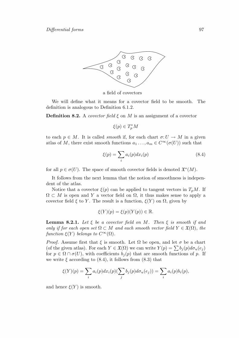
Differential forms 97

a field of covectors

We will define what it means for a covector field to be smooth. Thedefinition is analogous to Definition 6.1.2.

Definition 8.2. A covector field ξ on M is an assignment of a covector

ξ(p) ∈ T ∗pM

to each p ∈ M . It is called smooth if, for each chart σ:U → M in a givenatlas of M , there exist smooth functions a1 . . . , am ∈ C∞(σ(U)) such that

ξ(p) =∑

i

ai(p)dxi(p) (8.4)

for all p ∈ σ(U). The space of smooth covector fields is denoted X∗(M).

It follows from the next lemma that the notion of smoothness is indepen-dent of the atlas.

Notice that a covector ξ(p) can be applied to tangent vectors in TpM . IfΩ ⊂ M is open and Y a vector field on Ω, it thus makes sense to apply acovector field ξ to Y . The result is a function, ξ(Y ) on Ω, given by

ξ(Y )(p) = ξ(p)(Y (p)) ∈ R.

Lemma 8.2.1. Let ξ be a covector field on M . Then ξ is smooth if andonly if for each open set Ω ⊂M and each smooth vector field Y ∈ X(Ω), thefunction ξ(Y ) belongs to C∞(Ω).

Proof. Assume first that ξ is smooth. Let Ω be open, and let σ be a chart(of the given atlas). For each Y ∈ X(Ω) we can write Y (p) =

∑

bj(p)dσu(ej)for p ∈ Ω ∩ σ(U), with coefficients bj(p) that are smooth functions of p. Ifwe write ξ according to (8.4), it follows from (8.3) that

ξ(Y )(p) =∑

i

ai(p)dxi(p)(∑

j

bj(p)dσu(ej)) =∑

i

ai(p)bi(p),

and hence ξ(Y ) is smooth.

98 Chapter 8

Conversely, assume that ξ(Y ) ∈ C∞(Ω) for all Ω and all Y ∈ X(Ω).In particular, we can take Ω = σ(U) and Y = dσ(ei) for a given chart,and conclude that the function ai defined by ai(p) = ξ(p)(dσu(ei)) dependssmoothly on p. By applying (7.1) to the covector ξ(p) and the dual bases(8.1)-(8.2) in Lemma 8.1 we see that (8.4) holds. Hence ξ is smooth.

Notice that if ξ is a smooth covector field onM , and ϕ ∈ C∞(M) a smoothfunction, then the covector field ϕξ defined by the pointwise multiplication(ϕξ)(p) = ϕ(p)ξ(p) for each p, is again smooth. This follows from Definition8.2, since the coefficients of ϕξ in (8.4) are just those of ξ, multiplied by ϕ.

If f ∈ C∞(M) then the differential df is a covector field, as it is explainedin Example 8.1.

Lemma 8.2.2. If f ∈ C∞(M) then df is a smooth covector field on M . Foreach chart σ on M , the expression for df by means of the basis (8.2) is

df =m

∑

i=1

∂(f σ)

∂uidxi. (8.5)

The differentials satisfy the rule d(fg) = g df + f dg for all f, g ∈ C∞(M).

Proof. The smoothness of df follows from (8.5), because the coefficient func-tions are smooth. The rule for the differential of fg also follows from (8.5),by means of the Leibniz rule for the partial differentiation of a product. Thuswe only need to prove this equality.

In order to do that we first note that by the chain rule,

dfp(dσu(ej)) = d(f σ)u(ej) =∂(f σ)

∂uj(u).

By applying (7.1) to the covector dfp and the dual bases (8.1)-(8.2) we obtainthe following expression from which (8.5) then follows

dfp =∑

i

dfp(dσu(ei))dxi(p).

Example 8.2 Let M = R2 with coordinates (x1, x2), and let f ∈ C∞(R2).Then the differential of f is given by (8.5) as

df =∂f

∂x1dx1 +

∂f

∂x2dx2,

and an arbitrary smooth covector field is given by

ξ = a1 dx1 + a2 dx2


with a1, a2 ∈ C∞(R2). A covector field which has the form df for somefunction f is said to be exact. It is a well-known result that ξ is exact if andonly if it is closed, that is, if and only if

∂a1

∂x2=∂a2

∂x1. (8.6)

That this is a necessary condition follows immediately from the fact that

∂2f

∂x1∂x2=

∂2f

∂x2∂x1. (8.7)

We will sketch the proof that (8.6) is also sufficient. Let a closed formξ = a1 dx1 + a2 dx2 on R2 be given. Choose a function f1 ∈ C∞(R2) with∂f1

∂x1= a1 (for example, f1(x1, x2) =

∫ x1

0a1(t, x2) dt). It follows from (8.6)

and (8.7) that ∂a2

∂x1= ∂2f1

∂x1∂x2. We deduce that a2 − ∂f1

∂x2does not depend on

x1, and choose a one-variable function f2 ∈ C∞(R) with f ′2 = a2 − ∂f1

∂x2, as a

function of x2. It is easily seen that f(x1, x2) = f1(x1, x2) + f2(x2) satisfies

both a1 = ∂f∂x1

and a2 = ∂f∂x2

.The analogous result is not valid in an arbitrary 2-dimensional manifold

(for example, it fails on M = R2 \ (0, 0)).

8.3 Differential forms

The notion of a covector field can be generalized to a notion of fields ofk-forms. Recall from Definition 7.4 that we denote by Ak(V ) the space ofalternating k-tensors on the vector space V . Recall also that A0(V ) = R andA1(V ) = V ∗, and if ξ1, . . . , ξm is a basis for V ∗, then a basis for Ak(V ) isobtained from the set of elements

ξi1 ∧ · · · ∧ ξik

where 1 ≤ i1 < · · · < ik ≤ m (see Theorem 7.4).

Definition 8.3.1. A k-form ω on M is an assignment of an element

ω(p) ∈ Ak(TpM)

to each p ∈M .

In particular, given a chart σ:U → M , the elements dxi1 ∧ · · · ∧ dxik,

where 1 ≤ i1 < · · · < ik ≤ m, are k-forms on the open subset σ(U) of M .For each p ∈ σ(U), a basis for Ak(TpM) is obtained from these elements.Therefore, every k-form ω on M has a unique expression on σ(U),

ω =∑

I=i1,...,ik

aI dxi1 ∧ · · · ∧ dxik

100 Chapter 8

where aI : σ(U) → R.

Definition 8.3.2. We call ω smooth if all the functions aI are smooth, foreach chart σ in an atlas of M . A smooth k-form is also called a differentialk-form. The space of differential k-forms on M is denoted Ak(M).

In particular, since A0(TpM) = R, we have A0(M) = C∞(M), that is, adifferential 0-form on M is just a smooth function ϕ ∈ C∞(M). Likewise, adifferential 1-form is nothing but a smooth covector field.

It can be verified, analogously to Lemma 8.2.1, that a k-form ω is smooth ifand only if ω(X1, . . . , Xk) ∈ C∞(Ω) for all open sets Ω and all X1, . . . , Xk ∈X(M). In particular, it follows that the notion of smoothness of a k-form isindependent of the chosen atlas for M .

Example 8.3 Let S be an oriented surface in R3. The volume form on Sis the 2-form defined by ωp(X1, X2) = (X1 ×X2) ·N for X, Y ∈ TpS, whereN ∈ R3 is the positive unit normal. In the local coordinates of a chart, it isgiven by

ω = (EG− F 2)1/2dx1 ∧ dx2

where E, F and G are the coefficients of the first fundamental form. Thevolume form is smooth, since these coefficients are smooth functions.

Lemma 8.3. Let ω be a k-form on M and ϕ a real function on M , anddefine the product ϕω pointwise by

ϕω(p) = ϕ(p)ω(p).

Then ϕω is a smooth k-form if ϕ and ω are smooth.Let θ be an l-form on M , and define the wedge product θ ∧ω pointwise by

(θ ∧ ω)(p) = θ(p) ∧ ω(p)

for each p. Then θ ∧ ω is a smooth k + l-form if ω and θ are smooth.

Proof. Easy.

8.4 Pull back

An important property of differential forms is that they can be pulled backby a map from one manifold to another. The construction is analogous tothat of the dual map in Section 7.2.

Definition 8.4. Let f :M → N be a smooth map of manifolds, and letω ∈ Ak(N). We define f∗ω ∈ Ak(M), called the pull back of ω, by

f∗ω(p)(v1, . . . , vk) = ω(f(p))(dfp(v1), . . . , dfp(vk))


for all v1, . . . , vk ∈ TpM and p ∈M .

It is easily seen that for each p ∈ M the operator f∗ω(p) so defined ismultilinear and alternating, so that it belongs to Ak(TpM). We have toverify that it depends smoothly on p. This will be done in the followinglemma. It is clear that f∗ω depends linearly on ω, this will be used in theproof of the lemma.

Let

ω =∑

I=i1,...,ik

aI dyi1 ∧ · · · ∧ dyik

be the expression for ω by means of the coordinates of a chart τ :V → Non N . Here yi is the i-th coordinate of τ−1 for i = 1, . . . , n, and I is anincreasing sequence of k numbers among 1, . . . , n.

Lemma 8.4.1. With notation from above,

f∗ω =∑

I

(aI f) d(yi1 f) ∧ · · · ∧ d(yik f) (8.8)

on f−1(τ(V )). In particular, f∗ω is smooth.

Proof. In view of Lemma 8.3, the last statement follows from (8.8), since allthe ingredients in this expression are smooth, and since M is covered by theopen subsets f−1(τ(V )), for all τ in an atlas of N .

In order to verify (8.8), it suffices to prove the following rules for pullbacks:

f∗(ϕω) = (ϕ f)f∗ω, (8.9)

f∗(θ ∧ ω) = f∗(θ) ∧ f∗(ω), (8.10)

f∗(dϕ) = d(ϕ f). (8.11)

These rules follow easily from the definitions.

In particular, Definition 8.4 allows us to define the restriction of a k-formon a manifold N to a submanifold M . Let i:M → N be the inclusion map,then we define ω|M = i∗ω. It is given at p ∈M simply by

ω|M (p)(v1, . . . , vk) = ω(p)(v1, . . . , vk)

for v1, . . . , vk ∈ TpM ⊂ TpN .The following result will be important later.

Lemma 8.4.2. Let f :M → N be a smooth map between two manifolds ofthe same dimension k. Let x1, . . . , xk denote the coordinate functions of a

102 Chapter 8

chart σ on M , and let y1, . . . , yk denote the coordinate functions of a chartτ on N . Then

f∗(dy1 ∧ · · · ∧ dyk) = det(df) dx1 ∧ · · · ∧ dxk (8.12)

where det(df) in p is the determinant of the matrix for dfp with respect tothe standard bases for TpM and Tf(p)N given by the charts.

Proof. The element f∗(dy1 ∧ · · · ∧ dyk) is a k-form on M , hence a constantmultiple of dx1 ∧ · · · ∧ dxk (recall that dimAk(V ) = 1 when dimV = k).We determine the constant by applying f∗(dy1 ∧ · · · ∧ dyk) to the vector(dσp(e1), . . . , dσp(ek)) in (TpM)k. We obtain, see (7.6),

f∗(dy1 ∧ · · · ∧ dyk)(dσp(e1), . . . , dσp(ek))

= (dy1 ∧ · · · ∧ dyk)(dfp(dσp(e1)), . . . , dfp(dσp(ek)))

=1

k!det(dyi(dfp(dσp(ej)))).

On the other hand, applying dx1 ∧ · · · ∧ dxk to the same vector in (TpM)k,we obtain, again by (7.6),

(dx1 ∧ · · · ∧ dxk)(dσp(e1), . . . , dσp(ek)) =1

k!det(δij) =

1

k!,

since dx1, . . . , dxk is the dual basis. It follows that the constant we areseeking is the determinant det(dyi(dfp(dσp(ej))))

Notice that dyi(dfp(dσp(ej))) are exactly the matrix elements for dfp. Theformula (8.12) now follows.

8.5 Exterior differentiation

In this section a differentiation operator d is defined for differential formson a smooth manifold M . It is a generalization of the operator which mapsa smooth function to its differential, in general it will map k-forms to k+ 1-forms. The operator simply consists of applying d to the coefficients aI inthe coordinate expression for the k-form.

Definition 8.5. Fix a chart σ:U → M , and let ω ∈ Ak(M). On its imageσ(U) ⊂M we can write

ω =∑

I

aI dxi1 ∧ · · · ∧ dxik(8.13)

where I = (i1, . . . , ik) with 1 ≤ i1 < · · · < ik ≤ m = dimM , and whereaI ∈ C∞(σ(U)) for each I (see below Definition 8.3.1). On the image σ(U)we then define

dω =∑

I

daI ∧ dxi1 ∧ · · · ∧ dxik, (8.14)


where daI is the differential of aI . Then dω ∈ Ak+1(σ(U)).

The operator d is called exterior differentiation. It is defined above byreference to a fixed chart σ, but we shall see in the following theorem thatit can be extended to a globally defined operator, which is independent ofany choice of chart or atlas. The theorem also mentions the most importantproperties of d.

Theorem 8.5. There exists a unique map d:Ak(M) → Ak+1(M) such that(8.14) holds on σ(U) for each chart σ in a given atlas for M . This map dis independent of the choice of the atlas. Furthermore, it has the followingproperties:

(a) if k = 0 it agrees with the differential d on functions,

(b) it is linear,

(c) d(ϕω) = dϕ ∧ ω + ϕdω for ϕ ∈ C∞(M), ω ∈ Ak(M),

(d) d(ω1∧ω2) = dω1 ∧ω2 +(−1)kω1 ∧ dω2 for ω1 ∈ Ak(M), ω2 ∈ Al(M),

(e) d(df1 ∧ · · · ∧ dfk) = 0 for all f1, . . . , fk ∈ C∞(M),

(f) d(dω) = 0 for all ω ∈ Ak(M).

Proof. Suppose an atlas is given. The map d is unique because (8.14) de-termines dω uniquely on σ(U), for each chart σ in the atlas. We have toverify the existence of d, the independency on the atlas, and the listed prop-erties. However, before we commence on this we shall prove that the chart-dependent operator of Definition 8.5 satisfies (a)-(f).

(a) Let k = 0 and ω = f ∈ C∞(M). The only summand in the expression(8.13) corresponds to I = ∅, and the coefficient a∅ is equal to f itself. Theexpression (8.14) then reads dω = df (on σ(U)).

(b) The coefficients aI in (8.13) depend linearly on ω, and the expression(8.14) is linear with respect to these coefficients, hence dω depends linearlyon ω.

(c) Let ϕ ∈ C∞(M), ω ∈ Ak(M), and write ω according to (8.13). Inthe corresponding expression for the product ϕω each coefficient aI is thenmultiplied by ϕ, and hence definition (8.14) for this product reads

d(ϕω) =∑

I

d(ϕaI) ∧ dxi1 ∧ · · · ∧ dxik

=∑

I

(aI dϕ+ ϕdaI) ∧ dxi1 ∧ · · · ∧ dxik

= dϕ ∧∑

I

aI dxi1 ∧ · · · ∧ dxik+ ϕ

∑

I

daI ∧ dxi1 ∧ · · · ∧ dxik

= dϕ ∧ ω + ϕdω

where the rule in Lemma 8.2.2 was applied in the second step.

104 Chapter 8

(d) Notice first that if I = (i1, . . . , ik) with 1 ≤ i1 < · · · < ik ≤ m then bydefinition

d(a dxi1 ∧ · · · ∧ dxik) = da ∧ dxi1 ∧ · · · ∧ dxik

(8.15)

for a ∈ C∞(M). The expression (8.15) holds also without the assumptionthat the indices i1, . . . , ik are increasingly ordered, for the dxi1 , . . . , dxik

canbe reordered at the cost of the same change of sign on both sides. Theexpression also holds if the indices are not distinct, because in that case bothsides are 0.

Let ω1 ∈ Ak(M), ω2 ∈ Al(M), and write both of these forms as follows,according to (8.13):

ω1 =∑

I

aI dxi1 ∧ · · · ∧ dxik, ω2 =

∑

J

bJ dxj1 ∧ · · · ∧ dxjl,

where I = (i1, . . . , ik) and J = (j1, . . . , jl). Then

ω1 ∧ ω2 =∑

I,J

aIbJdxi1 ∧ · · · ∧ dxik∧ dxj1 ∧ · · · ∧ dxjl

and hence according to the remarks just made

d(ω1 ∧ ω2) =∑

I,J

d(aIbJ) ∧ dxi1 ∧ · · · ∧ dxik∧ dxj1 ∧ · · · ∧ dxjl

=∑

I,J

(bJ daI + aI dbJ) ∧ dxi1 ∧ · · · ∧ dxik∧ dxj1 ∧ · · · ∧ dxjl

=∑

I,J

bJ daI ∧ dxi1 ∧ · · · ∧ dxik∧ dxj1 ∧ · · · ∧ dxjl

+∑

I,J

aI dbJ ∧ dxi1 ∧ · · · ∧ dxik∧ dxj1 ∧ · · · ∧ dxjl

= dω1 ∧ ω2 + (−1)kω1 ∧ dω2

where the sign (−1)k in the last step comes from passing dbJ to the rightpast the elements dxi1 up to dxik

.

(e) is proved first for k = 1. In this case f ∈ C∞(M) and

df =

m∑

i=1

∂(f σ)

∂xidxi.

Hence

d(df) =

m∑

i=1

d[∂(f σ)

∂xi

]

∧ dxi =

m∑

i=1

m∑

j=1

∂2(f σ)

∂xj∂xidxj ∧ dxi.


The latter expression vanishes because the coefficient ∂2(fσ)∂xj∂xi

= ∂2(fσ)∂xi∂xj

oc-

curs twice with opposite signs.The general case is now obtained by induction on k. It follows from

property (d) that d(df1∧· · ·∧dfk) can be written as a sum of two terms eachof which involve a factor where d is applied to a wedge product with fewerfactors. Applying the induction hypothesis, we infer the statement.

(f) Let ω be given by (8.13). Then

d(dω) = d(∑

I

daI ∧ dxi1 ∧ · · · ∧ dxik) = 0

by property (e).

Having established these properties for the operator d on σ(U), we proceedwith the definition of the global operator d. Let p ∈M be given and choosea chart σ around p. We define dω(p) for each ω ∈ Ak(M) by the expressionin Definition 8.5. We need to prove that dω(p) is independent of the choiceof chart (this will also establish the independency of the atlas).

Suppose d′ω is defined on σ′(U ′) for some other chart σ′. The claim isthat then d′ω = dω on the overlap σ′(U ′) ∩ σ(U) of the two charts.

Assume first that U ′ ⊂ U and σ′ = σ|U ′ . In the expression (8.13) forω on σ′(U ′) we then have the restriction of each aI to this set, and sinced(aI |σ′(U ′)) = daI |σ′(U ′) it follows that the expression (8.14) for d′ω on σ′(U ′)is just the restriction of the same expression for dω. Hence d′ω = dω on σ′(U ′)as claimed.

For the general case the observation we just made implies that we canreplace U by the open subset σ−1(σ′(U ′) ∩ σ(U)) and σ by its restriction tothis subset, without affecting dω on σ′(U ′)∩ σ(U). Likewise, we can replaceU ′ by σ′−1(σ′(U ′)∩σ(U)). The result is that we may assume σ(U) = σ′(U ′).Moreover, we can replace M by the open subset σ(U) = σ′(U ′), and ω by itsrestriction to this set, since this has no effect on the expressions (8.13) and(8.14). In conclusion, we may assume that σ(U) = σ′(U ′) = M .

We now apply the rules (a)-(f) for d to the expression

ω =∑

I

a′I dx′i1 ∧ · · · ∧ dx′ik

for ω with respect to the chart σ′. It follows from (b), (c) and (e) that

dω =∑

I

d(a′I dx′i1 ∧ · · · ∧ dx′ik

)

=∑

I

da′I ∧ dx′i1 ∧ · · · ∧ dx′ik,

and hence dω = d′ω as claimed.

106 Chapter 8

It is now clear that dω is a well defined smooth k+1-form. The properties(a)-(f) hold, since they hold for the restrictions to σ(U), for any chart σ.

As in Section 7.6 we define

A(M) = A0(M) ⊕A1(M) ⊕ · · · ⊕Am(M)

where m = dimM . The elements of A(M) are called differential forms. Thusa differential form is a map which associates to each point p ∈M a memberof the exterior algebra A(TpM), in a smooth manner. The operator d mapsthe space of differential forms to itself.

8.6 Some examples

In the following we treat M = Rn for various values of n. In each case wedenote by σ: Rn → Rn the standard chart on Rn, the identity map.

Example 8.6.1 Let M = R. Since dimM = 1, we have A(R) = A0(R) ⊕A1(R). Furthermore, A0(R) = C∞(R) and A1(R) = a dx | a ∈ C∞(R).The exterior differentiation is given by df = f ′ dx for f ∈ A0(R) and df = 0for f ∈ A1(R).

Example 8.6.2 Let M = R2. Since dimM = 2, we have

A(R2) = A0(R2) ⊕ A1(R2) ⊕A2(R2).

Furthermore, A0(R2) = C∞(R2) and

A1(R2) = a1 dx1 + a2 dx2 | a1, a2 ∈ C∞(R2)A2(R2) = a dx1 ∧ dx2 | a ∈ C∞(R2)

The exterior differentiation is given by

df =∂f

∂x1dx1 +

∂f

∂x2dx2

(see Example 8.2), and

d(a1 dx1+a2 dx2)

= da1 ∧ dx1 + da2 ∧ dx2

=

(

∂a1

∂x1dx1 +

∂a1

∂x2dx2

)

∧ dx1 +

(

∂a2

∂x1dx1 +

∂a2

∂x2dx2

)

∧ dx2

=

(

−∂a1

∂x2+∂a2

∂x1

)

dx1 ∧ dx2


Example 8.6.3 Let M = R3. Then

A(R3) = A0(R3) ⊕A1(R3) ⊕ A2(R3) ⊕ A3(R3).

Furthermore, A0(R2) = C∞(R2) and

A1(R3) = a1 dx1 + a2 dx2 + a3 dx3 | a1, a2, a3 ∈ C∞(R3)A2(R3) = b1dx2 ∧ dx3 + b2dx3 ∧ dx1 + b3dx1 ∧ dx2 | b1, b2, b3 ∈ C∞(R3)A3(R3) = a dx1 ∧ dx2 ∧ dx3 | a ∈ C∞(R3).

The exterior differentiation is given by

df =∂f

∂x1dx1 +

∂f

∂x2dx2 +

∂f

∂x3dx3

and

d(a1 dx1+a2 dx2 + a3 dx3)

= da1 ∧ dx1 + da2 ∧ dx2 + da3 ∧ dx3

=

(

∂a1

∂x1dx1 +

∂a1

∂x2dx2 +

∂a1

∂x3dx3

)

∧ dx1

+

(

∂a2

∂x1dx1 +

∂a2

∂x2dx2 +

∂a2

∂x3dx3

)

∧ dx2

+

(

∂a3

∂x1dx1 +

∂a3

∂x2dx2 +

∂a3

∂x3dx3

)

∧ dx3

=

(

∂a3

∂x2− ∂a2

∂x3

)

dx2 ∧ dx3

+

(

∂a1

∂x3− ∂a3

∂x1

)

dx3 ∧ dx1

+

(

∂a2

∂x1− ∂a1

∂x2

)

dx1 ∧ dx2

Furthermore,

d (b1dx2 ∧ dx3 + b2dx3 ∧ dx1 + b3dx1 ∧ dx2)

= db1 ∧ dx2 ∧ dx3 + db2 ∧ dx3 ∧ dx1 + db3 ∧ dx1 ∧ dx2

=

(

∂b1∂x1

+∂b2∂x2

+∂b3∂x3

)

dx1 ∧ dx2 ∧ dx3

andd(a dx1 ∧ dx2 ∧ dx3) = 0.

108 Chapter 8

The expressions that occur as coefficients of dω in the three degrees arefamiliar from vector calculus. The vector field

grad f =

(

∂f

∂x1,∂f

∂x2,∂f

∂x3

)

is the gradient of f , and the vector field

curl a =

(

∂a3

∂x2− ∂a2

∂x3,∂a1

∂x3− ∂a3

∂x1,∂a2

∂x1− ∂a1

∂x2

)

is the curl (or rotation) of a. Finally, the function

div b =∂b1∂x1

+∂b2∂x2

+∂b3∂x3

is the divergence of b.

8.7 Exterior differentiation and pull back

The following property of exterior differentiation plays an important rolein the next chapter.

Theorem 8.7. Let g:M → N be a smooth map of manifolds, and let

g∗:Ak(N) → Ak(M)

denote the pull-back, for each k (see Definition 8.4). Then

dM g∗ = g∗ dN ,

where dM and dN denotes the exterior differentiation for the two manifolds.

Proof. By Lemma 8.4.1, and properties (b), (c) and (e) above,

d(g∗ω) = d(∑

I

(aI g) d(yi1 g) ∧ · · · ∧ d(yik g))

=∑

I

d(aI g) ∧ d(yi1 g) ∧ · · · ∧ d(yik g).

On the other hand, by the properties of g∗ listed in the proof of Lemma 8.4.1,

g∗(dω) = g∗(∑

I

daI ∧ dyi1 ∧ · · · ∧ dyik)

=∑

I

d(aI g) ∧ d(yi1 g) ∧ · · · ∧ d(yik g).

Corollary 8.7. Let M be a submanifold of the abstract manifold N , and letω be a differential form on N . Then the restriction of ω to M is a differentialform on M , and it satisfies d(ω|M ) = dω|M , that is, exterior differentiationand restriction commute.

Proof. The restriction ω|M is exactly the pull back i∗ω by the inclusion mapi:M → N . The result is an immediate consequence of Theorem 8.7.

Chapter 9

Integration

The purpose of this chapter is to define integration on smooth manifolds,and establish its relation with the differentiation operator d of the previouschapter.

9.1 Null sets

Recall from Geometry 1 that a compact set D ⊂ R2 is said to be a nullset, if for each ǫ > 0 it can be covered by a finite union of rectangles withtotal area < ǫ. We will generalize this concept to subsets D of an abstractmanifold M .

We first treat the case of sets in Rn. The notion of a rectangle is generalizedas a box, by which we mean a product set D = I1 × · · · × In ⊂ Rn, whereeach Ii is a closed interval [ai, bi] with −∞ < ai ≤ bi < ∞. The volume ofD is the product of the lengths of the intervals. The box is called a cube ifthe intervals have equal length.

Definition 9.1.1. A set A ⊂ Rn is said to be a null set if for each ǫ > 0it can be covered by a countable collection of boxes, of which the sum ofvolumes is < ǫ.

It is clear that any subset of a null set is again a null set.

Example 9.1.1 Clearly a singleton A = x is a null set. More generallyevery countable subset of Rn is a null set, since we can cover it by countablymany boxes, each of volume 0.

Example 9.1.2 Let m < n and consider a set in Rn of the form

A = (x1, . . . , xm, 0, . . . , 0) | x ∈ Rm.

By writing Rm as a countable union of boxes Bi we can arrange that A iscovered by the boxes Bi × 0, all of volume 0.

In fact for our present purpose we need only consider compact sets A. Inthis case, we can replace the word countable by finite in the above definition.Indeed, suppose a compact set A is covered by countably many boxes withvolume sum < ǫ. By increasing each box slightly, say the volume of the i-thbox is increased at most by 2−iǫ, we can arrange that A is contained in acountable union of open boxes with volume sum < 2ǫ. By Definition 5.1.2,A is then covered by a finite subcollection, which of course also has volumesum < 2ǫ.

110 Chapter 9

Lemma 9.1.2. Let A ⊂ Rn be a null set, and let f :A → Rn be a smoothmap. Then f(A) is a null set.

Proof. We only give the proof for the case that A is compact. By Definition2.6.1, f has an extension F to a smooth map defined on an open set Wcontaining A. Let D ⊂ W be compact, then there exists an upper bound Con the absolute values of the first order derivatives of F over D. Using themean value theorem, one then obtains an estimate |F (x)− F (y)| ≤ C|x− y|for all x, y ∈ D. It follows from this estimate that the image by F of a ballinside D of radius r is contained in a ball of radius Cr.

Let ǫ > 0 be given and choose a finite collection of boxes, which cover Aand whose volumes add to < ǫ. By possibly increasing some of the boxesslightly, we can arrange that all the boxes have positive and rational sidelengths, still with volumes adding to < ǫ. We can then write each box as aunion of cubes of any size which divides the lengths of all sides of the box,and which only intersect along their boundary. We thus obtain a coveringof A by finitely many cubes, whose volumes add to < ǫ. The circumscribedball of a cube has a volume which is proportional to that of the cube, witha factor c that depends only on n. It follows that we can cover A by finitelymany arbitrarily small closed balls, whose volumes add to < cǫ. In particular,we may assume that each of these balls is contained in W . The discussionin the first part of the proof (with D equal to the union of the balls) thenimplies that f(A) is covered by finitely many balls of total volume < Cncǫ.By circumscribing these balls with cubes, we obtain a covering of F (A) byboxes as desired.

Definition 9.1.2. Let M be an abstract manifold of dimension m. Asubset A ⊂M is called a null set in M , if there exists a countable collectionof charts σi:Ui →M and null sets Ai ⊂ Ui such that A = ∪iσi(Ai).

In order for this to be a reasonable definition, we should prove that adiffeomorphism of open sets in Rm carries a null set to a null set, so thatthe condition on Ai is unchanged if σi is reparametrized. This follows fromLemma 9.1.2.

Example 9.1.3 Let N be a submanifold of M , with dimN < dimM , andassume that N has a countable atlas. Then N is a null set in M . It followsfrom Theorem 4.3 that for each p ∈ N there exists a chart σ on M aroundp, such that N ∩ σ(U) is the image of a null set in U (see Example 9.1.2). Acountable collection of these charts will already cover N , since N is secondcountable (see Lemma 2.9).

9.2 Integration on Rn

Recall from Geometry 1, Chapter 3, that a non-empty subset D ⊂ R2 iscalled an elementary domain if it is compact and if its boundary is a finite

Integration 111

union of smooth curves [a, b] → R2. If D is an elementary domain, U ⊂ R2

an open set and f :U → R a continuous function, the plane integral∫

Df dA

was given a sense in Geometry 1. The crucial property of D in this definitionis that D is compact and that its boundary is a null set. In particular, ifD = [a, b] × [c, d] is a rectangle,

∫

D

f dA =

∫ b

a

∫ d

c

f(u, v) dv du =

∫ d

c

∫ b

a

f(u, v) du dv.

These definitions can be generalized to Rn in analogous fashion. A non-empty compact subset D ⊂ Rn is called a domain of integration if its bound-ary is a null set in Rn. Assume that D is a domain of integration and thatD ⊂ U , where U is open. In this case, if f :U → R is continuous, the in-tegral

∫

Df dV can be given a sense. The details are omitted since they are

analogous to those in Geometry 1.In particular, if D = [a1, b1]×· · ·× [an, bn] is a generalized rectangle, then

∫

D

f dV =

∫ b1

a1

· · ·∫ bn

an

f(x1, . . . , xn) dxn . . . dx1,

and the order of the consecutive integrals over x1, . . . , xn can be interchangedfreely. Of course, for n = 1 the concept coincides with the ordinary integralof a continuous function if D is an interval. In the trivial case n = 0, whereRn = 0, we interprete the definition so that the integral over D = 0 off is the evaluation of f in 0.

Example 9.2.1 If Ω ⊂ Rn is bounded and is a domain with smooth bound-ary, then the closure D = Ω is a domain of integration. The boundary ∂Ω isan n− 1-dimensional manifold, hence a null set according to Example 9.1.3.

The integral∫

Df dV has the following properties, also in analogy with

the two-dimensional case:∫

D

f + g dA =

∫

D

f dA+

∫

D

g dA

∫

D

cf dA = c

∫

D

f dA

|∫

D

f dA | ≤∫

D

|f | dA∫

D1∪D2

f dA =

∫

D1

f dA+

∫

D2

f dA,

where in the last line D1 and D2 are domains of integration with disjointinteriors.

There is an important rule for change of variables, which reads as follows.It will not be proved here.

112 Chapter 9

Theorem 9.2. Let φ:U1 → U2 be a diffeomorphism of open sets, and letD ⊂ U1 be a domain of integration. Then φ(D) ⊂ U2 is a domain of inte-gration and

∫

φ(D)

f dV =

∫

D

(f φ) |det(Dφ)| dV

for all continuous f :U2 → R.

9.3 Integration on a chart

Let S ⊂ R3 be a surface, and let σ:U → M be a chart on it. If D ⊂ Uis a domain of integration, the area of the set R = σ(D) ⊂ M is definedas the integral

∫

D(EG − F 2)1/2 dA, where E, F , G are the coefficients of

the first fundamental form. It was shown in Geometry 1 that the area isindependent of the chosen parametrization σ, thanks to the presence of thefunction (EG−F 2)1/2. The Jacobian determinant that arises in a change ofcoordinates, is exactly compensated by the change of this square root whenE, F and G are replaced by their counterparts for the new coordinates.

Similarly, if f :S → R is a continuous function, its integral overR is definedto be

∫

R

f dA =

∫

D

(f σ) (EG− F 2)1/2 dA.

This integral is independent of the chart, for the same reason as before.These considerations can be generalized to an m-dimensional smooth sur-

face in Rk. The factor (EG− F 2)1/2 in the integral over D is generalized asthe square root of the determinant det(σ′

ui· σ′

uj), i, j = 1, . . . , m, for a given

chart σ. The dot is the scalar product from Rn.When trying to generalize further to an abstract m-dimensional manifold

M we encounter the problem that in general there is no dot product on TpM ,hence there is no way to generalize E, F and G. As a consequence, it is notpossible to define the integral of a function on M in a way that is invariantunder changes of of charts. One way out is to introduce the presence of aninner product on tangent spaces as an extra axiom in the definition of theconcept of a manifold - this leads to so-called Riemannian geometry, which isthe proper abstract framework for the theory of the first fundamental form.

Another solution is to replace the integrand including (EG− F 2)1/2 by adifferential form of the highest degree. This approach, which we shall followhere, leads to a theory of integration for m-forms, but not for functions.In particular, it does not lead to a definition of area, since that would beobtained from the integration of the constant 1, which is a function, not aform. However, we can still view the theory as a generalization to the theoryfor surfaces, by defining the integral of a function f over a surface as theintegral of f times the volume form (see Example 8.3).

Integration 113

For some applications it is important to be able to integrate forms whichare continuous, but not smooth. The definition of continuity of forms isanalogous to Definition 8.3.2: A continuous k-form on an abstract manifoldM is a k-form ω for which all the functions aI are continuous, for each chartin an atlas of M . In particular, an m-form on an m-dimensional manifoldthus has the form

ω = φdx1 ∧ · · · ∧ dxm (9.1)

on each chart σ, with φ a continuous function on σ(U).

Definition 9.3. LetM be anm-dimensional oriented abstract manifold, andlet σ:U → M be a positive chart on M . Let ω ∈ Am(M) be a continuousm-form on M . Let D ⊂ U be a domain of integration, and let R = σ(D).Then we define

∫

R

ω =

∫

D

φ σ dV (9.2)

where φ is the function determined in (9.1).

We shall now see that the definition is independent of the choice of chart.The point is that when coordinates are changed, the function φ that rep-resents ω changes by a factor that exactly compensates for the Jacobiandeterminant resulting from the change. The Jacobian determinant has sim-ply been built into the object that we integrate. This is the central ideabehind the theory.

Theorem 9.3. The integral∫

Rω is independent of the choice of positive

chart σ. More precisely, if R is contained in the image of some other chart,then the integral defined in (9.2) has the same value for the two charts.

Proof. The statement is the special case of the identity mapping M →M inthe following more general result.

Lemma 9.3. Let M , M be oriented abstract manifolds, and let g: M → Mbe an orientation preserving diffeomorphism. Let σ:U → M and σ: U → Mbe charts, and let D ⊂ U and D ⊂ U be domains of integration. Assume thatg(R) = R, where R = σ(D) and R = σ(D).

Furthermore, let ω be a continuous m-form on M and let ω = g∗ω be itspull back by g (defined as in Definition 8.5). Then

∫

R

ω =

∫

R

ω.

Proof. The open subset σ(U)∩g−1(σ(U)) of σ(U) contains R. Hence we can

replace σ by its restriction to the preimage in U of this set with no effecton the integral over R. That is, we may assume that σ(U) ⊂ g−1(σ(U)), or

equivalently, g(σ(U)) ⊂ σ(U).

114 Chapter 9

Similarly, since g(σ(U)) contains R, we can replace σ by its restriction tothe preimage in U of this set with no effect on the integral over R. In otherwords, we may in fact assume that g(σ(U)) = σ(U).

Let Φ denote the coordinate expression for g,

Φ = σ−1 g σ: U → U.

It is a diffeomorphism of U onto U . The claim is that∫

D

φ σ dV =

∫

D

φ σ dV

where ω = φdx1 ∧ · · · ∧ xm and ω = φ dx1 ∧ · · · ∧ xm are the expressions forω and ω.

It follows from Lemma 8.4.2 that

g∗(dx1 ∧ · · · ∧ dxm) = det(dg) dx1 ∧ · · · ∧ dxm, (9.3)

where det(dgp) is the determinant of the matrix for dgp with respect to thestandard bases for the tangent spaces. In other words, det(dgp) is the deter-minant of the Jacobian matrix DΦ of the coordinate expression Φ. Applying(8.9) and (9.3) we conclude that

ω = g∗ω = g∗(φdx1 ∧ · · · ∧ dxm) = (φ g) det(DΦ) dx1 ∧ · · · ∧ dxm.

It follows thatφ = det(DΦ) (φ g). (9.4)

Since D = Φ(D) we obtain from Theorem 9.2∫

D

φ σ dV =

∫

D

φ σ Φ |det(DΦ)| dV. (9.5)

Observe that σ Φ = g σ, and that det(DΦ) is positive since g preservesorientation. It now follows from (9.4) that the expression (9.5) equals

∫

D

φ σ dV,

and the lemma is proved.

Example 9.3 Let γ: I → R2 be an embedded parametrized curve, and letω be a continuous 1-form on R2, say ω = f1(x1, x2) dx1 + f2(x1, x2) dx2. Let[a, b] ⊂ I and R = γ([a, b]). Then

∫

R

ω =

∫ b

a

F (γ(u)) · γ′(u) du (9.6)

where F (x1, x2) = (f1(x1, x2), f2(x1, x2)). This is seen as follows. The basisfor the 1-dimensional tangent space of γ at p = γ(u) is γ′(u), and the dualbasis vector du(p) is defined by du(p)(γ′(u)) = 1. On the other hand, ωp(v) =F (p) ·v for v ∈ R2, and in particular ωp(γ

′(u)) = F (p) ·γ′(u). Hence ω|γ(I) =φdu with φ(p) = F (p) · γ′(u). Now (9.6) follows from Definition 9.3. Theexpression (9.6) is called the line integral of ω along R.

Integration 115

9.4 Integration on a manifold

We shall generalize the definition of∫

Rω to the case where R is not nec-

essarily contained inside a single chart.

Definition 9.4.1. A compact subset R of an abstract manifold M is saidto be a domain of integration, if the boundary ∂R is a null set.

For example, if Ω ⊂M is a domain with smooth boundary, such that theclosure R = Ω is compact, then this closure is a domain of integration, byCorollary 4.6 and Example 9.1.3.

It is easily seen that the union R1 ∪R2, the intersection R1 ∩R2 and theset difference R1 \ R

2, of two domains of integration R1, R2 ⊂ M is again adomain of integration (in all three cases, the boundary is contained in theunion of the boundaries of R1 and R2).

In particular, if R ⊂ M is a domain of integration, and if σ:U → M is achart with another domain of integration D ⊂ U , then σ(D)∩R is a domainof integration inside σ(U), to which we can apply the preceding definition ofthe integral. We shall define the integral over R as a sum of such integrals,for a collection of charts that cover R. In order to combine these integralsdefined by different charts, we employ a partition of unity, see Section 5.4.We therefore assume that M has a locally finite atlas.

We choose around each point p ∈ M a chart σ:U → M and a domainof integration D ⊂ U such that p is contained in the image σ(D) of theinterior. The collection of all these charts is denoted σα:Uα → M , where Ais the index set. The open sets σα(D

α) for all α ∈ A cover M . We choosea partition of unity (ϕα)α∈A such that each function ϕα has support insidethe corresponding set σ(D

α) (see Theorem 5.5). Notice that the collectionof the supports of the functions ϕα is locally finite, hence only finitely manyof these functions are non-zero on the compact set R.

Definition 9.4.2. Let ω and be a continuous m-form on M , and let R ⊂Mbe a domain of integration. We define

∫

R

ω =∑

α∈A

∫

R∩σα(Dα)

ϕαω,

where the integrals on the right are defined with respect to the charts σα, asin Definition 9.3. The sum is finite, since only finitely many ϕα are non-zeroon R.

Theorem 9.4. The definition given above is independent of the choice ofthe charts σα and the subsequent choice of a partition of unity.

Proof. Indeed, if ϕα, where α ∈ A, is a different partition of unity relative

116 Chapter 9

to a different atlas, then

∑

α∈A

∫

R∩σα(Dα)

ϕα ω =∑

α∈A

∫

R∩σα(Dα)

(∑

α∈A

ϕα)ϕα ω

=∑

α∈A

∑

α∈A

∫

R∩σα(Dα)

ϕαϕα ω

and since ϕαϕα ω is supported inside the intersection R∩ σα(Dα)∩ σα(Dα),the latter expression equals

∑

α∈A

∑

α∈A

∫

R∩σα(Dα)∩σα(Dα)

ϕαϕα ω

The integral over R∩σα(Dα)∩ σα(Dα) has the same value for the two chartsby Theorem 9.3. Hence the last expression above is symmetric with respectto the partitions indexed by A and A, and hence the original sum has thesame value if the partition is replaced by the other one.

It is easily seen that∫

Mω depends linearly on ω. Moreover, in analogy

with Lemma 9.3:

Lemma 9.4. Let g: M → M be an orientation preserving diffeomorphism,and R ⊂ M a domain of integration. Then R = g(R) ⊂ M is a domainof integration. Furthermore, let ω be a continuous m-form with pull backω = g∗ω. Then

∫

R

ω =

∫

R

ω.

Proof. Let (ϕα)α∈A be a partition of unity on M , as in Definition 9.4.2, and

put ψα = ϕα g ∈ C∞(M). Since g is a diffeomorphism, this is a partition

of unity on M . It follows from (8.9), that g∗(ϕαω) = ψαω. The proof is nowstraightforward from Definition 9.4.2 and Lemma 9.3.

The case of a 0-dimensional manifold needs special interpretation. Recallthat a 0-dimensional abstract manifold is a discrete set M . By definition, anorientation of M assigns + or − to each point in M , it can thus be viewed asa function o:M → +,−. A subset R is compact if and only if it is finite.A 0-form on M is a function f :M → R, and the interpretation of its integralover a finite set D is that it is the signed sum

∑

p∈D

o(p)f(p).

This interpretation may seem peculiar, but it is extremely convenient (forexample, in Example 9.6.1 below).

Integration 117

9.5 A useful formula

The definition of∫

Rω by means of a partition of unity is almost impossible

to apply, when it comes to explicit computations, because it is very difficultto write down explicit partitions of unity. The following theorem, of whichthe proof is omitted, can be used instead. The idea is to chop up R in finitelymany pieces and treat each of them separately. The pieces are chosen suchthat they are convenient for computations.

Theorem 9.5. Let M be an abstract oriented manifold, let ω be a continuousm-form on M , and let R ⊂M be a domain of integration.

a) Assume that R = R1 ∪ · · · ∪Rn where each set Ri ⊂M is a domain ofintegration, such that all the interiors R

i are disjoint from each other. Then

∫

R

ω =

n∑

i=1

∫

Ri

ω.

b) Let i = 1, . . . , n and assume that there exist an open set Ui ⊂ Rm,a smooth map gi:Ui → M and a domain of integration Di ⊂ Ui such thatRi = gi(Di), and such that the restriction gi|D

iis a positive chart. Then

∫

Ri

ω =

∫

Di

g∗i ω.

Let φi:Ui → R be the function determined by g∗i ω = φi du1 ∧ · · · ∧ dum,with u1, . . . , um the coordinates of Rm. Then the last formula above reads

∫

Ri

ω =

∫

Di

φi dV.

Notice that the requirement on the map gi is just that its restriction to theinterior of Di is a chart. If gi itself is a chart, σ = gi, then the presentfunction φi is identical with the function φ σ in (9.2), and the formula for∫

Riω by means of g∗i ω is identical with the one in Definition 9.3.

For example, the unit sphere S2 is covered in this fashion by a single mapg:D → S2 of spherical coordinates

g(u, v) = (cosu cos v, cosu sin v, sinu)

with D = [−π/2, π/2] × [−π, π], and thus we can compute the integral of a2-form over S2 by means of its pull-back by spherical coordinates, in spite ofthe fact that this is only a chart on a part of the sphere (the point being, ofcourse, that the remaining part is a null set).

118 Chapter 9

9.6 Stokes’ theorem

Stokes’ theorem is the central result in the theory of integration on man-ifolds. It gives the relation between exterior differentiation and integration,and it generalizes the fundamental theorem of calculus.

Let M be an m-dimensional oriented abstract manifold, and let Ω ⊂M bea domain with smooth boundary. The boundary ∂Ω (which may be empty)is equipped with the induced orientation, see Section 4.8. For example, Ωcould be the inside of a compact connected manifold in Rn, as in the Jordan-Brouwer theorem, Theorem 5.10.

As mentioned below Definition 9.4.1, if Ω is compact, then Ω is a domain ofintegration, and hence the integral

∫

Ωω is defined for all continuous m-forms

on M . The requirement that Ω is compact can be relaxed as follows. Observethat if R is a domain of integration, then so is the intersection Ω ∩ R, sincethe boundary of each set is a null set. Let now ω be a continuous m-form.The support suppω of ω is the closure of the set p ∈M | ω(p) 6= 0. Assumethat Ω∩suppω is compact, and choose a domain of integration R ⊂M whichcontains this set. We can then define the integral of ω over Ω (or Ω) by

∫

Ω

ω =

∫

Ω∩R

ω,

the point being that the right hand side is independent of the choice of R.

Theorem 9.6. Stokes’ theorem. Let ω be a differential m − 1-form onM , and assume that Ω ∩ suppω is compact. Then

∫

Ω

dω =

∫

∂Ω

ω. (9.7)

The right-hand side is interpreted as 0 if ∂Ω is empty.

The result is remarkable, because it shows that by knowing ω only on theboundary of Ω, we can predict a property of it on the interior, namely thetotal integral of its derivative.

Proof. Let R ⊂ M be a domain of integration containing Ω ∩ suppω. Thenthis set also contains Ω ∩ supp dω. Hence by definition

∫

Ω

dω =

∫

Ω∩R

dω and

∫

∂Ω

ω =

∫

∂Ω∩R

ω.

Choose around each point p ∈M a chart σ:U →M and an m-dimensionalrectangle D ⊂ U such that p ∈ σ(D), where D is the interior of D. Inaddition we assume that these charts are chosen so that if p ∈ ∂Ω thenσ(U) ∩ Ω = σ(U+) where U+ = x ∈ U | um > 0 (see Theorem 4.6), ifp ∈ Ω then σ(U) ⊂ Ω and if p ∈M \ Ω then σ(U) ⊂M \ Ω.

Integration 119

We may now assume that ω is supported inside σ(D) for one of thesecharts. For if the result has been established in this generality, we can applyit to ϕαω for each element ϕα in a partition of unity as in Definition 9.4.2.Since the set R is compact, only finitely many ϕα’s are non-zero on it, andas both sides of (9.7) depend linearly on ω, the general result then follows.

The equation (9.7) clearly holds if σ(U) ⊂ M \ Ω, since then both sidesare 0. This leaves the other two cases, σ(U) ∩ Ω = σ(U+) and σ(U) ⊂ Ω, tobe checked.

We may also assume that

ω = f dx1 ∧ · · · ∧ dxj−1 ∧ dxj+1 ∧ · · · ∧ dxm

for some j between 1 and m, because in general ω will be a sum of suchforms.

Since df =∑m

i=1∂f∂xi

dxi (see Lemma 8.2.2), it then follows that

dω = (−1)j−1 ∂f

∂xjdx1 ∧ · · · ∧ dxm,

where the sign appears because dxj has been moved past the 1-forms fromdx1 up to dxj−1.

Assume first that j < m. We will prove that then

∫

Ω

dω =

∫

∂Ω

ω = 0.

By definition

∫

Ω

dω = (−1)j−1

∫

Ω

∂f

∂xjdx1 ∧ · · · ∧ dxm = (−1)j−1

∫

∂(f σ)

∂ujdV,

where the last integration takes place over the set x ∈ D | σ(x) ∈ Ω, that

is, over D ∩ U+ or D, in the two cases.In the integral over the rectangle D ∩U+ or D, we can freely interchange

the order of integrations over u1, . . . , um. Let us take the integral over uj

first (innermost), and let us denote its limits by a and b. Notice that sincej < m these are the limits for the uj variable both in D ∩ U+ and D. Nowby the fundamental theorem of calculus

∫ b

a

∂(f σ)

∂ujduj = f(σ(u1, . . . , uj−1, b, uj+1, . . . , um))

− f(σ(u1, . . . , uj−1, a, uj+1, . . . , um)).

However, since ω is supported in σ(D), it follows that these values are zerofor all u1, . . . uj−1, uj+1, . . . um, and hence

∫

Ωdω = 0 as claimed.

120 Chapter 9

On the other hand, if σ(U)∩Ω = σ(U+), then xm = 0 along the boundary,and it follows immediately that dxm, and hence also ω, restricts to zero on∂Ω. Therefore also

∫

∂Ωω = 0. The same conclusion holds trivially in the

other case, σ(U) ⊂ Ω.

Next we assume j = m. Again we obtain 0 on both sides of (9.7) in thecase σ(U) ⊂ Ω, and we therefore assume the other case. We will prove thatthen

∫

Ω

dω =

∫

∂Ω

ω = (−1)m

∫

f(σ(u1, . . . , um−1, 0)) du1 . . . dum−1,

where the integral runs over the set of (u1, . . . , um−1) ∈ Rm−1 for whichσ(u1, . . . , um−1, 0) ∈ ∂Ω

Following the preceding computation of∫

Ωdω, we take the integral over

uj = um first. This time, however, the lower limit a is replaced by the value0 of xm on the boundary, and the previous conclusion fails, that f vanisheshere. Instead we obtain the value f(σ(u1, . . . , um−1, 0)), with a minus infront because it is the lower limit in the integral. Recall that there was afactor (−1)j−1 = (−1)m−1 in front. Performing the integral over the othervariables as well, we thus obtain the desired integral expression

(−1)m

∫

f(σ(u1, . . . , um−1, 0)) du1 . . . dum−1

for∫

Ωdω.

On the other hand, the integral∫

∂Ωω can be computed by means of the

restricted chart σ|U∩Rm−1 on ∂Ω. However, we have to keep track of theorientation of this chart. By definition (see Section 4.8), the orientation ofthe basis

dσ(e1), . . . , dσ(em−1)

for Tp∂M is the same as the orientation of the basis

−dσ(em), dσ(e1), . . . , dσ(em−1)

for TpM . The orientation of the latter is (−1)m, because σ is a positivechart. It follows that

∫

∂Ω

ω = (−1)m

∫

f(σ(u1, . . . , um−1, 0)) du1 . . . dum−1,

as claimed.

Integration 121

9.7 Examples from vector calculus

In the following examples we always use the standard coordinates on theEuclidean space Rn.

Example 9.6.1. Let M = R, then m = 1 and ω is a 0-form, that is, afunction f ∈ C∞(R). The differential of f is the 1-form df = f ′(x)dx (seeExample 8.6.1). Let Ω =]a, b[, then the boundary ∂Ω consists of the twopoints a and b, oriented by −1 and +1, respectively (see Example 4.7.3).Hence

∫

Ω

dω =

∫ b

a

df =

∫ b

a

f ′(x) dx

and∫

∂Ω

ω = f(b) − f(a)

Thus we see that in this case Stokes’ theorem reduces to the fundamentaltheorem of calculus.

Example 9.6.2. Let M = R2, then m = 2 and ω is a 1-form. The boundaryof the open set Ω is a union of smooth curves, we assume for simplicity itis a single simple closed curve. Write ω = f(x, y) dx+ g(x, y) dy, then (seeExample 8.6.2)

dω = (−∂f∂y

+∂g

∂x) dx ∧ dy

and hence∫

Ω

dω =

∫

Ω

−∂f∂y

+∂g

∂xdA.


∂Ωω over the boundary can be computed

as follows. Assume γ: [0, T ] → ∂Ω is the boundary curve, with end pointsγ(0) = γ(T ) (and no other self intersections). Theorem 9.5 can be appliedwith D1 = [0, T ] and g1 = γ. Write γ(t) = (x(t), y(t)), then by definition

g∗1ω = (f γ) d(x γ) + (g γ) d(y γ),

and∫

∂Ωω is the line integral

∫

∂Ω

ω =

∫

γ

f(x, y)dx+ g(x, y)dy.

We thus see that in this case Stokes’ theorem reduces to the classical Green’stheorem (which is equivalent with the divergence theorem for the plane):

∫

Ω

−∂f∂y

+∂g

∂xdA =

∫

γ

f(x, y)dx+ g(x, y)dy.

122 Chapter 9

The orientation of γ is determined as follows. If n and t are the outwardnormal vector and the positive unit tangent vector, respectively, in a givenpoint of γ, then (n, t) should be positively oriented, that is, t = n, which isexactly the standard counter clockwise orientation of a closed curve in R2.

Example 9.6.3. Let M = R3, and let Ω be a domain with smooth bound-ary. The boundary ∂Ω is then a surface S in R3. Let ω be a 2-form onM :

ω = f(x, y, z) dy ∧ dz + g(x, y, z) dz ∧ dx+ h(x, y, z) dx ∧ dy.Then (see Example 8.6.3)

dω = (∂f

∂x+∂g

∂y+∂h

∂z) dx ∧ dy ∧ dz

and hence∫

Ω

dω =

∫

Ω

div(f, g, h) dV,

where div(f, g, h) = ∂f∂x

+ ∂g∂y

+ ∂h∂z

is the divergence of the vector field (f, g, h).


∂Ωω over the boundary ∂Ω = S can

be computed as follows. Suppose D1, . . . , Dn and gi:Di → S are as inProposition 9.5 for the manifold S. Then

∫

S ω =∑n

i=1

∫

Dig∗i ω. Let σ(u, v) =

gi(u, v) be one of the functions gi. Then

σ∗ω = (fσ) d(yσ)∧d(zσ)+(gσ) d(zσ)∧d(xσ)+(fσ) d(xσ)∧d(yσ).

Furthermore

d(y σ) ∧ d(z σ) = (∂σ2

∂udu+

∂σ2

∂vdv) ∧ (

∂σ3

∂udu+

∂σ3

∂vdv)

= (∂σ2

∂u

∂σ3

∂v− ∂σ2

∂v

∂σ3

∂u) du ∧ dv

and similarly

d(z σ) ∧ d(x σ) = (∂σ3

∂u

∂σ1

∂v− ∂σ1

∂v

∂σ3

∂u) du ∧ dv

d(x σ) ∧ d(y σ) = (∂σ1

∂u

∂σ2

∂v− ∂σ2

∂v

∂σ1

∂u) du ∧ dv.

Notice that the three expressions in front of du∧dv are exactly the coordinatesof the normal vector σ′

u × σ′v. Thus we see that

σ∗ω = (f σ, g σ, h σ) · (σ′u × σ′

v) du ∧ dv.

Let N(u, v) denote the outward unit normal vector in σ(u, v), then σ′u×σ′

v =‖σ′

u × σ′v‖N and we see that

∫

Dσ∗ω is the surface integral of the function

Integration 123

(f, g, h) · N over the image of σ = gi (recall that the surface integral ofa function includes a factor ‖σ′

u × σ′v‖ = (EG − F 2)1/2). Summing over

i = 1, . . . , n we finally obtain the surface integral

∫

S

ω =

∫

S

(f, g, h) · N dA.

We conclude that in this case Stokes’ theorem reduces to the divergencetheorem (sometimes also called the Gauss theorem):

∫

Ω

div(f, g, h) dV =

∫

∂Ω

(f, g, h) · N dA.

Example 9.6.4. Let M = S be an oriented smooth surface in R3, and letΩ ⊂ M be a domain with smooth boundary. Let ω be a 1-form on M , andassume ω is the restriction of a smooth 1-form

f(x, y, z) dx+ g(x, y, z) dy+ h(x, y, z) dz

defined on an open neighborhood of M in R3. A similar analysis as in theprevious example shows that in this case Stokes’ theorem reduces to theoriginal theorem of Stokes, which is

∫

Ω

(curlF ·N) dA =

∫

∂Ω

f dx+ g dy + h dz.

where

curlF = (∂h

∂y− ∂g

∂z,∂f

∂z− ∂h

∂x,∂g

∂x− ∂f

∂y).

The preceding examples show that in addition to the fundamental theo-rem of calculus, Stokes’ theorem also generalizes the three main theorems ofclassical vector calculus.

124 Chapter 9

Index

algebraic variety, 11alternating, 89

form, 90ambient space, 10atlas, 8, 17

compatible, 18countable, 27

base, for topology, 27basis, standard, 40boundary, 16

orientation, 54bump function, 60chain rule, 37, 39chart, 8closed

set, 16vector field, 99

closure, 16compact, 57compatible, 18component, 68connected, 64

component, 68continuous, 16contravariant, 89coordinate

expression, 30, 32function, 74, 96map, 11

cotangent space, 95countable,

atlas, 27second, 27

covariant, 87covector, 95

field , 97cover, 8covering, 57

open, 57critical value, 49curl, 108curve, 5

diffeomorphism, 21, 24differential, 38,

form, 100dimension of manifold, 1, 10, 18directional derivative, 35, 36, 37discrete

set, 10topology, 16

divergence, div, 108theorem, 123

domainof integration, 111, 115with smooth boundary, 52

dualbasis, 85map, 86vector space, 85

Einstein convention, 89embedded

parametrized manifold, 3submanifold, 55

embedding, 56exact vector field, 99extension, local 21exterior

algebra, 94differentiation, 103

Gauss, 123GL(n,R), 26gl(n,R), 81, 83gradient, grad, 108Green, 121group, Lie, 25

orthogonal, 51Hausdorff topology, 17Heine-Borel property, 57homomorphism, Lie, 84homeomorphism, 3, 17immersed submanifold, 55immersion, 56induced topology, 17integral, 111, 113, 115

126 Index

interior, 16intermediate value property, 64isolated point, 10Jacobi identity, 79Jordan-Brouwer theorem, 69Jordan curve theorem, 69k-form, 99left translation, 80left invariant, 80level set, 49Lie

algebra, 81bracket, 77group, 25homomorphism, 84

locally finite, 59manifold,

abstract, 18embedded parametrized, 3in Rn, 10parametrized, 1product, 20

map,continuous, 16smooth, 21, 22, 24

mixed tensor, 89Mobius band, 42multilinear, 87neighborhood, 16null set, 109, 110O(n), 51, 84o(n), 84open, 15

covering, 57relatively, 3, 17

orientable, 41, 69orientation, 41

of boundary,54preserving, 41

oriented, 41,orthogonal group, O(n), 51parametrized curve on, 30, 32partition of unity, 61

pathwise connected, 64locally, 67

productmanifold, 20topology, 20

projection, 75pull back, 100regular, 1

value, 49relatively open, 3, 17reparametrization, 2restriction, of k-form, 101second countable, 27smooth,

atlas, 17boundary, 52covector field, 97differential form, 100extension, 21map, 21, 22, 24structure, 18vector field, 71, 72

space,ambient, 10Hausdorff, 17projective, 19tangent, 30, 29, 32tensor, 87topological, 15

standard basis, 40Stokes’ theorem, 118, 123structure, smooth, 18subcovering, 57submanifold, 43, 44

structure, 48embedded, 55immersed, 55

support, 61surface, 7tangent

bundle, 75map, 37space, 30, 29, 32

Index 127

tangential, 32tensor, 87

contravariant, 89covariant, 87mixed, 89product, 88space, 87

topological space, 15topology,

discrete, 16Hausdorff, 17trivial, 16

value,critical, 49regular, 49

variety, 11vector,

cotangent, 95field, 71tangent, 32

volume form, 100wedge product, 92Whitney’s theorem, 28, 62

Lecture Notes for Geometry 2 Henrik Schlichtkrullweb.math.ku.dk/~jakobsen/geom2/manusgeom2.pdf ·...

Documents

Transcript of Lecture Notes for Geometry 2 Henrik Schlichtkrullweb.math.ku.dk/~jakobsen/geom2/manusgeom2.pdf ·...