Lecture Notes

Compuational Physics

(part of Mathematical Methods & ComputationalPhysics: PH33008/PH43018)

S. Murugesh

January 19, 2009

Contents

1 Differential equations: 31.1 Euler method . . . . . . . . . . . . . . . . . . . . . . . . . . . . . . . . . . . . . . . 31.2 Runge-Kutta method(s) . . . . . . . . . . . . . . . . . . . . . . . . . . . . . . . . . 4

2 Projectiles 62.1 The cyclist: without resistance . . . . . . . . . . . . . . . . . . . . . . . . . . . . . . 62.2 The cyclist: with resistance . . . . . . . . . . . . . . . . . . . . . . . . . . . . . . . 62.3 2-D projectile motion . . . . . . . . . . . . . . . . . . . . . . . . . . . . . . . . . . . 72.4 Projectile including air resistance . . . . . . . . . . . . . . . . . . . . . . . . . . . . 72.5 Projectile with density correction at high altitudes . . . . . . . . . . . . . . . . . . . 82.6 Motion of a batted baseball: Effect of velocity dependent drag, and wind . . . . . . 82.7 Motion of pitched baseball (knuckleball): Effect of spin . . . . . . . . . . . . . . . . 92.8 Trajectory of a Golf ball: . . . . . . . . . . . . . . . . . . . . . . . . . . . . . . . . . 10

3 Oscillatory motion and Chaos 123.1 Simple harmonic motion: . . . . . . . . . . . . . . . . . . . . . . . . . . . . . . . . . 123.2 Driven nonlinear pendulum: Chaos . . . . . . . . . . . . . . . . . . . . . . . . . . . 133.3 Poincare section . . . . . . . . . . . . . . . . . . . . . . . . . . . . . . . . . . . . . . 143.4 Period doubling map: Route to chaos . . . . . . . . . . . . . . . . . . . . . . . . . . 143.5 The Lorenz model . . . . . . . . . . . . . . . . . . . . . . . . . . . . . . . . . . . . . 143.6 The Billiard problem . . . . . . . . . . . . . . . . . . . . . . . . . . . . . . . . . . . 153.7 Bouncing balls . . . . . . . . . . . . . . . . . . . . . . . . . . . . . . . . . . . . . . . 15

4 The solar system 244.1 Kepler’s laws . . . . . . . . . . . . . . . . . . . . . . . . . . . . . . . . . . . . . . . 244.2 Precession of the perihelion of Mercury . . . . . . . . . . . . . . . . . . . . . . . . . 244.3 The three-body problem: Effect of Jupiter on the orbit of Earth . . . . . . . . . . . 264.4 Resonances in the Solar system: Kirkwood Gaps and Planetary Rings . . . . . . . . 264.5 Chaotic tumbling of Hyperion . . . . . . . . . . . . . . . . . . . . . . . . . . . . . . 27

5 Potentials and Fields 295.1 Laplace’s equation (Relaxation methods) . . . . . . . . . . . . . . . . . . . . . . . . 295.2 Poisson’s equation . . . . . . . . . . . . . . . . . . . . . . . . . . . . . . . . . . . . 305.3 Magnetic field due to a current . . . . . . . . . . . . . . . . . . . . . . . . . . . . . 30

1

5.4 Simpsons’ rule . . . . . . . . . . . . . . . . . . . . . . . . . . . . . . . . . . . . . . . 31

6 Wave motion 326.1 Simple wave equation . . . . . . . . . . . . . . . . . . . . . . . . . . . . . . . . . . . 326.2 Spectral methods . . . . . . . . . . . . . . . . . . . . . . . . . . . . . . . . . . . . . 33

7 Random systems 347.1 Random number generator . . . . . . . . . . . . . . . . . . . . . . . . . . . . . . . . 347.2 A different choice of distribution . . . . . . . . . . . . . . . . . . . . . . . . . . . . . 357.3 Monte Carlo integration . . . . . . . . . . . . . . . . . . . . . . . . . . . . . . . . . 357.4 The Random walk problem . . . . . . . . . . . . . . . . . . . . . . . . . . . . . . . . 367.5 Self avoiding walk(SAW) . . . . . . . . . . . . . . . . . . . . . . . . . . . . . . . . . 367.6 Random walk and diffusion . . . . . . . . . . . . . . . . . . . . . . . . . . . . . . . 377.7 Random walk in 2-D and Entropy . . . . . . . . . . . . . . . . . . . . . . . . . . . . 387.8 Cluster growth models . . . . . . . . . . . . . . . . . . . . . . . . . . . . . . . . . . 387.9 Fractals and Fractal dimensionality of curves . . . . . . . . . . . . . . . . . . . . . . 397.10 Percolation . . . . . . . . . . . . . . . . . . . . . . . . . . . . . . . . . . . . . . . . 40

8 Statistical Mechanics 448.1 The Ising Model . . . . . . . . . . . . . . . . . . . . . . . . . . . . . . . . . . . . . . 448.2 Mean field theory . . . . . . . . . . . . . . . . . . . . . . . . . . . . . . . . . . . . . 448.3 Newton’s method . . . . . . . . . . . . . . . . . . . . . . . . . . . . . . . . . . . . . 468.4 The Monte Carlo Method . . . . . . . . . . . . . . . . . . . . . . . . . . . . . . . . 46

2

Chapter 1

Differential equations:

Note: Usual notations

yx =dy

dx; yxxxxxxxxxx =

d10y

dx10= y10x

1.1 Euler method

First step in solving differential equations. Consider

yt = F (y(t), t) ; y(t0) = y0. (1.1)

Recall

yt(t) = lim∆τ→0

y(t + ∆τ) − y(t)

∆τ(1.2)

≃ y(t + ∆τ) − y(t)

∆τ(1.3)

for small values of ∆τ . So,y(t + ∆τ) = y(t) + ∆τyt(t). (1.4)

Ory(t0 + ∆τ) = y(t0) + ∆τyt(t)|t0 . (1.5)

= y(t0) + ∆τF (y(t0), t0) (1.6)

for small values of ∆τ .Alternatively, recall Taylor expansion for y(t) around t (for small ∆τ):

y(t + ∆τ) = y(t) + yt(t)∆τ +1

2ytt∆τ 2 +

1

6y3t∆τ 3 + .... (1.7)

→ agrees with Eq. (1.5) to first order in ∆τ . So error in Euler method is of order ∆τ 2.Pictorially, Euler method is shown in Figure 1. Euler method uses slope at the point t0 to

extrapolate y(t0 + ∆τ).

3

errory

t0t

∆τ

Figure 1.1: Euler method: Using y(t0) and the slope (yt(t0)), Euler method estimates y(t0 +∆τ) asy(t0) + yt(t0)∆τ . This agrees with Taylor series up to first order in ∆τ . Thus error is of order ∆τ 2.

1.2 Runge-Kutta method(s)

A more accurate method comes by choosing an intermediate point in the ′t′ interval, say ∆τ/2, tocalculate the slope, i.e., F (y, t). The catch: to calculate y(t0 + ∆τ

2) use Euler method. So

Step 1:

y(t0 +∆τ

2) = y(t0) + F (y(t0), t0)∆τ. (1.8)

Step2:

y(t0 + ∆τ) = y(t0) + yt(t0 +∆τ

2)∆τ (1.9)

= y(t0) + F (y(t0 +∆τ

2), t0 +

∆τ

2)∆τ.

Or, in conformity with texts,Step 1:

K1 = F (y(t0), t0)∆τ (1.10)

Step 2:

K2 = F (y(t0) +K1

2, t0 +

∆τ

2)∆τ (1.11)

y(t0 + ∆τ) = y(t0) + K2. (1.12)

This is the Two-step(for obvious reasons) Runge-Kutta method.Exercise 1.1 Find out the order of error in this method, upon comparing with Taylor series.

Higher order methods follow on similar lines using more intermediate points to calculate theslope, with the Four-step RK method (or Fourth order RK method) being the preferred choice:

4

K1 = F (y(t0), t0)∆τ (1.13)

K2 = F (y(t0) +K1

2, t0 +

∆τ

2)∆τ (1.14)

K3 = F (y(t0) +K2

2, t0 +

∆τ

2)∆τ (1.15)

K4 = F (y(0) + K3, t0 + ∆τ)∆τ (1.16)

y(t0 + ∆τ) = y(t0) +1

6(K1 + 2K2 + 2K3 + K4) (1.17)

Exercise 2.2 Radioactive decay is governed by the equation

dN

dt= −N

τ, (1.18)

where N(t) is the number of nuclei of the radioactive material at time ′t′ and τ is the time constantfor the decay. Choosing N(0) = 100 and τ = 1, simulate Eq. (1.18) and compare with the analyticalsolution (How else can you verify?).

Exercnse 2.3 Extend the scheme suggested by Euler’s method to a) Coupled system of ODEs,b) Higher order ODEs and c) PDEs.

5

Chapter 2

Projectiles

2.1 The cyclist: without resistance

Consider equation of motion

vt =F

m(2.1)

for a bicycle of velocity v(t) and mass (including cyclist) m. F is the force acting on the bicycle,due to the cyclist’s effort. Assume, horizontal road, and no resistance (anywhere). F is difficultto calculate. Let P be the power a cyclist can provide (can be roughly calculated experimentally).Then

P = Et, (2.2)

where E is the energy of the bicycle-cyclist combo. Road being horizontal, E = mv2/2. Thus

P = mvvt, (2.3)

or

vt =P

mv. (2.4)

If P is constant then, if v(0) = v0,

v =√

v20 + 2Pt/m. (2.5)

Exercise 2.1: Verify Eq. (2.5).

Eq. (2.5) implies v increases indefinitely with time. Cannot be true.Exercise 2.2: Numerically simulate Eq. (2.4), assuming P = 400W (constant!), and other

values reasonably.

2.2 The cyclist: with resistance

Assume air resistance of the formFdrag = B1v + B2v

2 (2.6)

6

vt =P

mv− Fdrag (2.7)

It turns out this is more significant compared to other resistance, such as friction between movingparts of the bicycle. The first term in Eq. (2.6) is the familiar Stokes’ law behavior. The secondterm is naturally the next possible significant term (recall Taylor expansion). For large velocitiesthe second term dominates. Roughly

B2 = ρA/2, (2.8)

where ρ is the density of air and A the frontal area of the cyclist-bicycle combo.The mass of air displaced by the cyclist ρAvdt, carrying a K.E ρAvdt · v2/2. This equals the

work done by Fdrag(= Fdrag · vdt).

Fdrag · vdt =mair

2v2 (2.9)

= ρAvdt · v2

2. (2.10)

So Eq. (2.4) modifies to (omitting the Stokes’ term)

vt =P

mv− ρA

2mv2. (2.11)

Exercise 2.3: Numerically plot the velocity of the cyclist using Eq. (2.11) for the same valuesfor the parameters, and compare with the results for Exercise 2.2.

2.3 2-D projectile motion

Consider projectile motion in 2-D - tracing the horizontal(x) and vertical(y) coordinates. Theequation of motion is the system of two differential equations

xtt = 0 ; ytt = −g. (2.12)

Or,xt = vx (2.13)

vxt = 0, (2.14)

yt = vy, (2.15)

vyt = −g. (2.16)

Note: In vx and vy, the subscripts are not derivatives.Exercise 2.4: Trace the projective described by the Eqs. (2.13-2.16), using Euler/R-K4 meth-

ods, choosing suitable initial values.Check if max range happens at angle of inclination of 45o.

7

2.4 Projectile including air resistance

Recall air resistance given byFdrag = B2v

2 ; v2 = v2x + v2

y . (2.17)

Evidently,

Fdrag,x = Fdragvx

v(2.18)

Fdrag,y = Fdragvy

v. (2.19)

Here again, subscripts do not denote derivativesSo, the modified equations are

xt = vx (2.20)

vxt = −B2

mvvx, (2.21)

yt = vy, (2.22)

vyt = −g − B2

mvvy. (2.23)

Exercise 2.5: Repeat Exercise 2.4 for Eqs. (2.20-2.23), choosing a reasonable value for B2(=ρA/2).

2.5 Projectile with density correction at high altitudes

In Eq. (2.23) B2 depends on ρ. At high altitudes, however, ρ is low. Infact

ρ = ρ0 exp(−y/y0) (2.24)

with y0 = 1.0 × 104 m.Exercise 2.6: Repeat Exercise 2.5 for the same values, but incorporating density correction.

Study carefully how the results vary.

2.6 Motion of a batted baseball: Effect of velocity depen-

dent drag, and wind

Base ball motion is complicated by the behavior of the ball with the speed. The behavior of thedrag coefficient C(B2 = CρA) is given in Figure 2.1 (a rough sketch). The drag when air flow issmooth is more, and less when the air around the ball is turbulent. For a rough ball, the turbulentphase sets in at much lower velocities, while for a smooth ball this happens at high velocities.

An exact analytical function for the above form is nontrivial. However, numerically, the behaviorfor a normal baseball is reasonably well described by

B2

m= 0.0039 +

0.0058

1 + exp[(v − vd)/∆], (2.25)

8

0

0 20010050 150

0.6

0.4

0.2

(miles per hour)v

Dra

g C

oeff

icie

nt

smooth ball

normalbaseball

rough baseball

Figure 2.1: Behavior of the drag coefficient C is shown above for three different types of baseballs.A rough ball can cause the air around it to be turbulent at much lower velocities, compared to asmooth baseball. Note that for low velocities the coefficient is roughly 0.5, as was the case from ourarguement for the cyclist.

where vd = 35 m/s and ∆ = 5 m/s.Add to this the effect of wind, assuming the wind to be blowing horizontally, and having a

constant magnitude and direction during the flight of the ball. Then (see Eq. (2.21) and Eq.(2.23)),

Fdrag,x = −B2|~v − ~vwind|(vx − vwind), (2.26)

Fdrag,y = −B2|~v − ~vwind|vy. (2.27)

Exercise 2.7: Trace the trajectories of a normal baseball, a) in vacuum, b) with a wind drag.Repeat the same assuming a wind speed of 10mph. Of particular interest is the angle of maximumrange, and the form of the trajectory. m = 149g.

9

2.7 Motion of pitched baseball (knuckleball): Effect of spin

While all the features of the previous section follows for a pitched baseball, the primary differenceis the effect of spin. It turns out that the force on the ball due to its spin is the most significant inchanging its trajectory. The force can be understood from the drag force Fdrag on the two sides ofthe ball. Let y axis, as earlier, be the direction of vertical. Consider the baseball moving along thex axis with velocity v, and spinning with the axis along y as shown in the Figure 2.2.

z

x

v−ωr

v+ ωr

Fv

ω

r

F

drag

Magnus

Figure 2.2: Schematic picture of the spinning ball, and the relative velocity on the two sides withrespect to the wind. This leads to a difference in the drag force on the two sides, effectively leadingto the Magnus force FMagnus in the −z direction. y axis is the vertical direction, which is also thedirection of spin.

From the figureFMagnus = −S0ωvxz ; (S0~ω × ~v in general), (2.28)

and the trajectory is 3-dimensional. So the equations become

xt = vx (2.29)

vxt = −B2

mvvx, (2.30)

yt = vy, (2.31)

vyt = −g (2.32)

zt = vz, (2.33)

10

vzt = −S0ωvx

m. (2.34)

Experimentally, S0/m(≈ 4.1 × 1)−4, where m = 149g.

2.8 Trajectory of a Golf ball:

Little change in detail, the spin is along the z axis. Thus the trajectory is 2-D with equations givenby:

xt = vx (2.35)

vxt = −B2

mvvx −

S0ωvy

m, (2.36)

yt = vy, (2.37)

vyt = −B2

mvvy +

S0ωvx

m− g. (2.38)

Recall, B2 = CρA. Experimentally,

C = 0.5 : v < 14m/s (2.39)

= 7/v : v > 14m/s

S0ω/m = 0.25s−1. (2.40)

Exercise 2.8:Consider a cricket ball bowled along the x direction, with its seam in the x − yplane, with y along the vertical. One side of the ball is assumed to be smooth compared to theother. If the ball is bowled with a backspin (angular velocity along z direction), sketch a rough forcediagram, and write down the equations of motion for the ball. Which direction do you expect theswing to be?

Suggested reading: See the short writeup on The physics of football in Physics World, June1, 1998: http://physicsworld.com/cws/article/print/1533

11

Chapter 3

Oscillatory motion and Chaos

Notation:

y =dy

dt;

...y =

d3y

dt3= y3t

3.1 Simple harmonic motion:

θ

Fθ

Figure 3.1: A simple pendulum. As long as oscillations remain small, the equation of motion isFθ = −mgθ. Otherwise, Fθ = −mg sin θ, a more complex nonlinear system. In particular, theperiod of the nonlinear pendulum is not 2π

√

l/g.

12

From Newton:θ = −g

lθ. (3.1)

Solutionθ = θ0 sin(Ωt + φ) (3.2)

Numerical implementation: Rewrite the II order ODE as two first order ODE

θ = ω (3.3)

ω = −g

lθ (3.4)

Exercise 3.1: Use methods discussed in Section 1 to numerically study the dynamics of thesimple pendulum Eq. (3.3) and Eq. (3.4). How does the results from the two - Runge-Kutta andEuler - methods compare? The system is conservative with energy being the conserved quantity. Usethis to check your numerical results. Also, compare with the analytical solution.

Exercise 3.2: How does the behavior change when θ in Eq. (3.4) is changed to sin θ. Onceagain, use (the new expression for) energy, the conserved quantity, to check your results.

3.2 Driven nonlinear pendulum: Chaos

Deterministic systems have a predictable future, i.e., given the initial condition and forces on thesystem, the future of the system is determined. However, the system may be sensitively dependenton the initial conditions that predictions over long time is practically impossible without “precise”knowledge of the initial conditions. Simple example: A tossed coin, or dice. Nevertheless, given theforces and initial condition “precisely”, the future of the system is “precisely” and “uniquely” deter-mined. Two trajectories, very close to start with, can deviate away from each other exponentially intime, that soon they lose any semblance, owing to their sensitive dependence on initial condition- afundamental feature of Chaos. An example can be found in the driven nonlinear damped pendulum

θ = −g

lsin θ − qθ + FD sin(ΩDt). (3.5)

Exercise 3.3: Taking l = g = 9.8, q = 1/2 and ΩD = 2/3, obtain the trajectories of θ(t), ω(t)for FD = 0, FD = 0.5 and FD = 1.2 (See Figure 3.2). Note: −π ≤ θ < π. Take ’modulus’ everytime θ goes above π.

Notice that the system has two periods, the characteristic period T = 2π√

l/g for small oscilla-tions, and frequency of the driving force ΩD. In the absence of the driving force, the system relaxesto a stop, θ = 0, due to the dissipation term. As the driving force FD is increased (0.5) the systemshows periodic motion, with period ΩD of the driving force. On further increasing FD(= 1.2), thesystem shows chaotic behavior.

Exercise 3.4: Consider two driven nonlinear pendulum θ1 and θ2 obeying the same dynamicalequation, Eq. (3.5), with all parameters same, but differing slightly in their initial conditions. Let∆θ = |θ1 − θ2|. Plot ∆θ vs t for the values FD = 0.5 and FD = 1.2.

13

Exercise 3.5: Notice that for FD = 1.2 in Exercise 3.4 the trajectory θ vs t is chaotic. RepeatExercise 3.4 for different choices of (θ1, θ2). Plot average ∆θ vs t, and find the slope of the linejoining the maxima. The slope is the Lyapunov exponent of the system. Notice that it is +ve whenFD = 1.2 and −ve when FD = 0.5. A positive Lyapunov exponent signifies Chaos.

Exercise 3.6: Using results from Exercise 3.4, plot the phase-space trajectories, i.e., ω vs θ(See Figure 3.3).

3.3 Poincare section

For FD = 0.5, the system shows periodic behavior, and for large values of FD, it shows chaoticbehavior. Given that the system has a characteristic time period due to ΩD, we can look atsnapshots of the system, a stroboscopic plot, taken at regular intervals of time 2π/ΩD. Thisstroboscopic phase-space plot in the characteristic time period of the system is known as Poincaresection or a Poincare surface. For a periodic system, such as Eq. (3.5) for FD = 0.5, this is justa point in the ω − θ plane. For a chaotic system, the Poincare map shows more structure and, isthe same for a wide range of initial conditions. The system starting in any initial condition willsooner or later reach one of these points, and thus have the same same Poincaree surface. Thusfor a chaotic system, the Poincare section is an invariant for a system, irrespective of the initialcondition. I.e., no matter what the initial condition, after a transient phase, the system goes into aphase such that the Poincare section is the same. For this reason we say the surface is an attractor.For the periodic case, the surface is just a point. For the chaotic regime, the structure is morecomplex, referred to as the strange attractor.

Exercise 3.7: Plot the Poincare surface for the forced pendulum in the chaotic regime (SeeFigure 3.4). Change initial condition to confirm if the surface remains invariant.

3.4 Period doubling map: Route to chaos

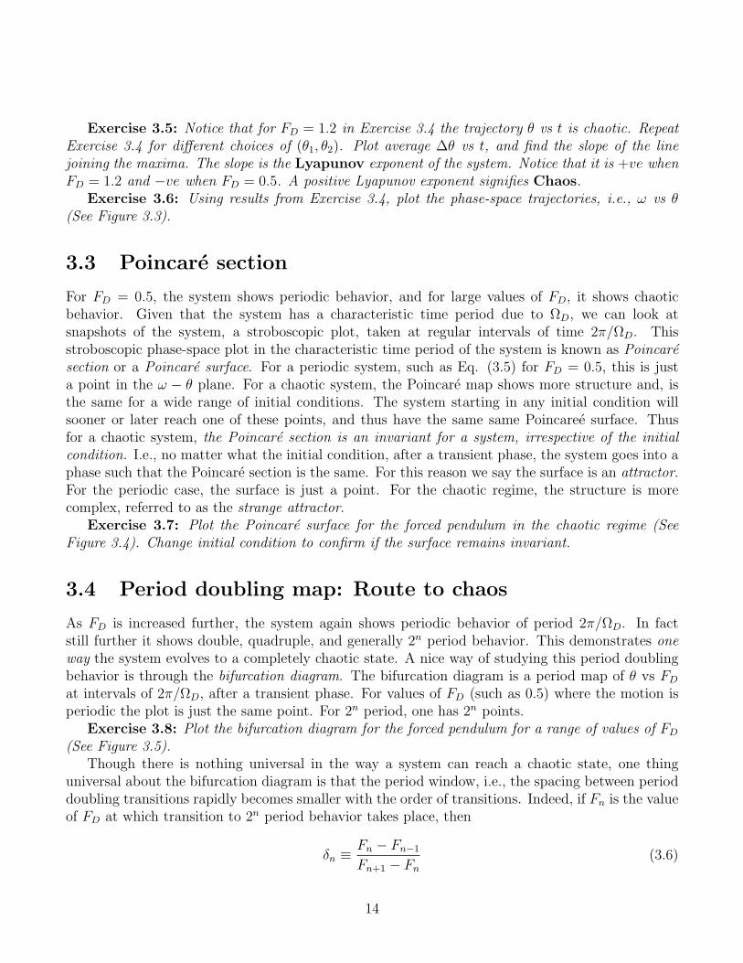
As FD is increased further, the system again shows periodic behavior of period 2π/ΩD. In factstill further it shows double, quadruple, and generally 2n period behavior. This demonstrates oneway the system evolves to a completely chaotic state. A nice way of studying this period doublingbehavior is through the bifurcation diagram. The bifurcation diagram is a period map of θ vs FD

at intervals of 2π/ΩD, after a transient phase. For values of FD (such as 0.5) where the motion isperiodic the plot is just the same point. For 2n period, one has 2n points.

Exercise 3.8: Plot the bifurcation diagram for the forced pendulum for a range of values of FD

(See Figure 3.5).Though there is nothing universal in the way a system can reach a chaotic state, one thing

universal about the bifurcation diagram is that the period window, i.e., the spacing between perioddoubling transitions rapidly becomes smaller with the order of transitions. Indeed, if Fn is the valueof FD at which transition to 2n period behavior takes place, then

δn ≡ Fn − Fn−1

Fn+1 − Fn

(3.6)

14

approaches the Feigenbaum number (= 4.669..) for large n.Exercise 3.9: Using the bifurcation diagram obtained in Exercise 3.8, verify that δn approaches

the Feigenbaum number.

3.5 The Lorenz model

The Lorenz model is an oversimplified version of the Navier-Stokes equation applied to the case ofReyleigh-Benard convection. Consider a fluid in a container with top and bottom surfaces held atdifferent temperatures. As the difference in temperatures is slowly increased, the fluid goes from astationary state, to steady flow (nonzero velocity field, but constant in time), to chaotic flow. Theequations around the steady state are reduced to

x = σ(y − x), (3.7)

y = −xz + rx − y, (3.8)

z = xy − bz. (3.9)

Due to comparisons with a simplified model of the atmosphere, the Lorenz model is also referredto as the weather problem.

Exercise 3.10: Show that the projection of the phase space plot in the x − z plane has thebutterfly structure shown below. The parameter values are σ = 10, b = 8/3 and r = 25 (See Figure3.6).

Exercise 3.11: Obtain the Poincare surface for the Lorenz model. Note that the system doesnot have a characteristic time period. The surface in this case is just the set of points on a planethat intersects the three dimensional trajectory, say, parallel to the x−z plane at y = 0 (See Figures3.7 & 3.8).

3.6 The Billiard problem

Consider the trajectory of a billiard ball in a perfectly reflecting table. The motion is assumed tobe frictionless, and the reflections are elastic. The equations are

x = vx, (3.10)

y = vy. (3.11)

At the point of reflection the tangential component of velocity is preserved, while the normalcomponent is reversed. A typical trajectory for a square table is shown in Figure 3.9. The characterof motion is governed by the shape of the table. In the case of a square and circular table the motionis noted to be periodic. A stadium is described as two halfs of a circle of radius r separated by adistance 2αr. The stadium billiard is chaotic for any nonzero value of α.

Exercise 3.12: Simulate the trajectories of the billiard in the case of square, circle and stadiumtables, and obtain the Poincare surfaces.

15

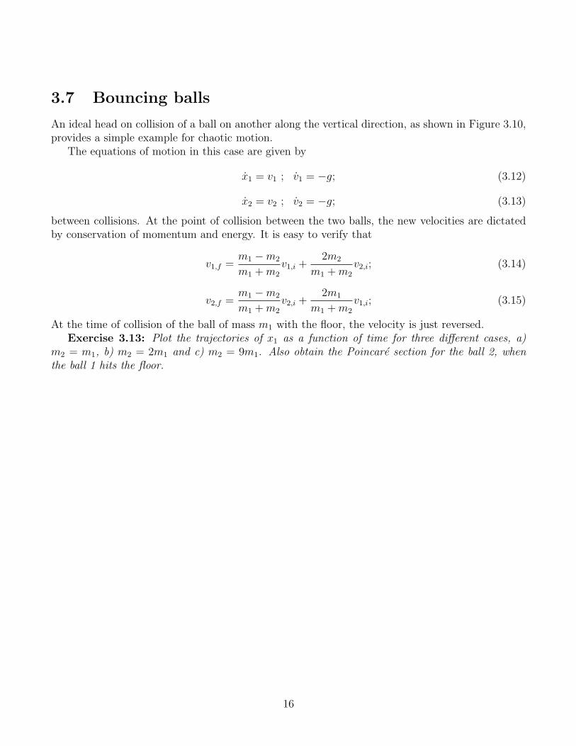
3.7 Bouncing balls

An ideal head on collision of a ball on another along the vertical direction, as shown in Figure 3.10,provides a simple example for chaotic motion.

The equations of motion in this case are given by

x1 = v1 ; v1 = −g; (3.12)

x2 = v2 ; v2 = −g; (3.13)

between collisions. At the point of collision between the two balls, the new velocities are dictatedby conservation of momentum and energy. It is easy to verify that

v1,f =m1 − m2

m1 + m2

v1,i +2m2

m1 + m2

v2,i; (3.14)

v2,f =m1 − m2

m1 + m2

v2,i +2m1

m1 + m2

v1,i; (3.15)

At the time of collision of the ball of mass m1 with the floor, the velocity is just reversed.Exercise 3.13: Plot the trajectories of x1 as a function of time for three different cases, a)

m2 = m1, b) m2 = 2m1 and c) m2 = 9m1. Also obtain the Poincare section for the ball 2, whenthe ball 1 hits the floor.

16

-12

-10

-8

-6

-4

-2

0

2

0 10 20 30 40 50 60

θ

t

(c)

FD=1.2

-4

-3

-2

-1

0

1

2

3

4

0 10 20 30 40 50 60

θ

t

(c)FD=1.2

-1

-0.5

0

0.5

1

0 10 20 30 40 50 60

θ

t

(b)

FD=0.5

-0.1

-0.05

0

0.05

0.1

0.15

0.2

0.25

0 10 20 30 40 50 60

θ

t

(a)

FD=0.0

Figure 3.2: The trajectories of θ in time for three different values of the driving force. In (c), theabrupt jumps are due to the modulus on θ (−π ≤ θ < π). (d) is the same as (c), but without themodulus.

17

-2

-1

0

1

2

-4 -3 -2 -1 0 1 2 3 4ω

θ

(b)

FD=1.2

-0.8

-0.6

-0.4

-0.2

0

0.2

0.4

0.6

0.8

-1 -0.5 0 0.5 1

ω

θ

(a)FD=0.5

Figure 3.3: Poincare surface for the driven pendulum at FD = 1.2. (ω, θ) values at intervals of2π/ΩD, the period of the driving force. The plot is independent of the initial condition.

-2

-1.5

-1

-0.5

0

0.5

1

-4 -3 -2 -1 0 1 2 3 4

ω

θ

FD=1.2

Figure 3.4: Poincare surface for the driven pendulum at FD = 1.2. (ω, θ) values at intervals of2π/ΩD, the period of the driving force. The plot is independent of the initial condition.

18

1

1.5

2

2.5

3

1.36 1.38 1.4 1.42 1.44 1.46 1.48 1.5

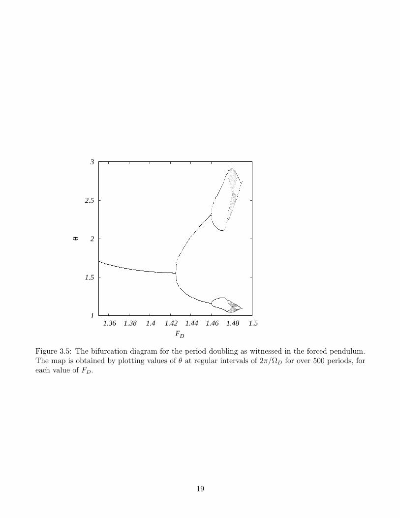
θ

FD

Figure 3.5: The bifurcation diagram for the period doubling as witnessed in the forced pendulum.The map is obtained by plotting values of θ at regular intervals of 2π/ΩD for over 500 periods, foreach value of FD.

19

0

5

10

15

20

25

30

35

40

45

-20 -15 -10 -5 0 5 10 15 20

z

x

Figure 3.6: The Butterfly obtained as a phase portrait for the Lorenz model. The portrait is aprojection in the x − z plane of the three dimensional trajectory in the x − y − z phase space.The parameter values are σ = 10, b = 8/3 and r = 25. The initial conditions chosen werex = 1, y = 0 = z.

20

-20-15-10 -5 0 5 10 15 20-20

-10 0

10 20

0 5

10 15 20 25 30 35 40 45

z

x

y

z

Figure 3.7: The trajectory in phase space for the Lorenz model for the same parametric values andinitial conditions as in Figure 3.6. The Poincare surface is the collection of points on the planeparallel to x − z plane, that intersects the trajectory at y = 0 (See Figure 3.8).

21

0

5

10

15

20

25

30

35

40

-15 -10 -5 0 5 10 15

z

x

Figure 3.8: The trajectory in phase space for the Lorenz model for the same parametric values andinitial conditions as in Figure 3.6. The Poincare surface is the collection of points on the planeparallel to x − z plane, that intersects the trajectory at y = 0 (See Figure 3.8).

-4

-2

0

2

4

-4 -2 0 2 4

vx

x

(b)

-4

-2

0

2

4

-4 -2 0 2 4

y

x

(a)

Figure 3.9: The trajectory of a billiard ball in a square billiard (a), with initial values x = 0.2, y =0, vx = 3 and vy = 2.2, and the Poincare surface. The Poincare section is a plot in the vx −x space,when y = 0.

22

m 2

m 1

g

Figure 3.10: A ball of mass m2 bounces head on from another ball of mass m1, which in turnbounces of the floor. The collisions are assumed to be elastic, and ideally along the vertical. Thesystem exhibits chaos depending on the ratio of the two masses.

23

Chapter 4

The solar system

In this chapter we look at tracking orbits of celestial bodies, and some related issues, numerically.

4.1 Kepler’s laws

First off, motion of a planet around the Sun. The Sun is assumed to be massive enough comparedto the planet (so it is!!), that we consider it to be fixed at the origin. The equations of motion forthe planet are

x = vx ; vx = −GMS

r2· x

r(4.1)

y = vy ; vy = −GMS

r2· y

r(4.2)

Its worthwhile going to astronomical units, length in AU (1AU = 1 × 1011 m, roughly thedistance between Earth and Sun), and time in years. We know, for Earth, assuming circular orbit,

GMSME

r2=

MEv2

r(4.3)

⇒ GMS = 4π2, (4.4)

in astronomical units (MS = 2 × 1030Kg,ME = 6 × 1024Kg).Exercise 4.1: Obtain the orbits of Earth around the Sun, by appropriately choosing initial

conditions for circular and elliptic orbits.Exercise 4.2: Using the results obtained in Exercise 4.1 verify Kepler’s laws of planetary

motion.Exercise 4.3: Without asking too many questions repeat exercises 4.1 and 4.2, assuming New-

ton’s law were 1/r2+β, for β = .001, .01, and .1, rest all remaining same.

4.2 Precession of the perihelion of Mercury

Exercise 4.3, would’ve illustrated an unstable behavior of the orbit, wherein the orbit is seen toprecess. A precession in the orbit of Mercury was a long standing fixation in celestial mechanics.

24

FF

F

x y

x

y

θ

G

Sun

Earth

Figure 4.1: A schematic diagram showing the orbit of Earth around the Sun.

It was noticed that the orbit of Mercury precesses 566 arcsecs per century (1 arcsec = 1/3600 de-grees). The Newton’s law cannot be of the form 1/r2+β, (β 6= 0), for various reasons. An alternateexplanation was the effect of gravitational field of other planets on Mercury. This accounted for523 arcsecs/century (This calculation was done by hand in the middle of 19th century). The remain-ing 43 arcsecs were explained by the general theory of relativity, and was one more confirmation ofthe general theory itself. The force law according to general theory is

FG ≈ GMSMM

r2(1 +

α

r2) (4.5)

where α ≈ 1.1 × 10−8AU2. To study the behavior numerically for such a small value of α is notviable. The precession of the perihelion of Mercury due to the modified force law is calculated asfollows:

1. Consider an elliptic orbit with semimajor axis a = 0.39 AU and eccentricity e = 0.206. Usingconservation of energy and angular momentum, the velocity at aphelion can be obtained as

v =

√

GMS(1 − e)

a(1 + e). (4.6)

2. Obtain the orbital trajectory for a fictional value of α, say 0.1.

3. A precessing orbit implies an aphelion (or perihelion) whose coordinate is changing with everyrevolution. Note down these coordinates (or angle), where the radial distance of Mercury from

25

the Sun is maximum (or minimum). Plot these extremal angle vs time. This is a straightline. The slope of this line gives the angular velocity, say ωα, with which the orbit precesses,for the chosen value of α.

4. Repeat step 3 for different values of α, to obtain a set of values of ωα for the correspondingvalues of α.

5. Plot ωα vs α. This, again, is a straight line (why?). Find its slope dωα/dα.

6. Using the slope obtained in the previous step, the precession for the real value of α is justα × dωα/dα.

Exercise 4.4: Obtain the expression for velocity v, shown in step 1 above, at the aphelion.

Exercise 4.5: Do steps 1 through 6 numerically, and show that the precession is indeed themissing 43 arcsecs/century (and thus provide the third supporting evidence for the generaltheory of relativity).

Exercise 4.6: You could not have demonstrated this crucial confirmation of general theoryso easily (as a text book exercise) had it not been for the straight line ωα vs α. Why is it astraight line?

4.3 The three-body problem: Effect of Jupiter on the orbit

of Earth

So far we have looked at problems of the two-body central force kind. Here we look at the effect ofthe presence of an additional planet in the system, on the orbits of the first planet. We consider theSun, Earth and Jupiter. The additional term in the scene is the force between Jupiter and Earth.

FEJ =GMJME

r2EJ

(4.7)

In component form (See Figure)

FEJ , x = −GMJME

r2EJ

cos θEJ − GMJME

r2EJ

(xE − xJ)

rEJ

. (4.8)

FEJ , y = −GMJME

r2EJ

cos θEJ − GMJME

r2EJ

(yE − yJ)

rEJ

. (4.9)

Use GMJ = GMS(MJ/MS) = 4π2MJ/MS, (MJ = 1.9 × 1027Kg) and radius 5.20 AU .Exercise 4.7: Making these modifications in the force equation for the two planets, study the

trajectories of Earth and Jupiter around the Sun. Letting the mass of Jupiter to vary, at what ratioof MJ/ME is there any perceivable difference in the orbit of the Earth? Try MJ → 1000 MJ .

26

4.4 Resonances in the Solar system: Kirkwood Gaps and

Planetary Rings

A curios hypothesis (a reminder of the way they did science those days) was the Titus-Bode formula(some time in the 18th century) for the radius of each planet, proposed without any scientific basiswhatsoever. Hypothesis: The radius of planets around the Sun (in AU) were the related to theterms in the series Sn = 0, 3, 6, 12, 24, ... as rn = (Sn +4)/10. This prediction agrees well for the firstfour planets. After a gap at n = 5 it agreed for Jupiter (n = 6) and Saturn. Uranus was discoveredlater (a search partially motivated by the Titus-Bode hypothesis). It does not agree so well forNeptune and Pluto however. The absence of any planet at n = 5 was a botheration. After severalpersistent searches for a missing planet, something was indeed observed at around 1800. But soonobservations of several similar objects followed. These were realized as not planets really, and werenamed asteroids.

The explanation for the absence is the following. The radius of the orbit around the sun isalso related to the period of the planet. The gap occurs at a radial distance such that the orbitalperiod is half that of Jupiter. Implying that Jupiter’s closest approach (and hence it significantgravitational pull) on such a planet will be at the same point on the planets orbit. Over severalorbits, this distorts its orbit severely that eventually the planet’s orbit is unstable. A smaller orlarger orbit will not however face this problem, since the periods may not have such a simple ratio.

A correspondence of such gaps in the solar system can be seen with the sub system of Saturn andits moons. Due to Saturn’s several moons, some orbits (or orbital radii) are not allowed. Objects insuch an orbit will be pushed to take either a smaller or a larger orbit. This explains the phenomenonof several rings around Saturn, which are just a collection of celestial dust bodies in orbital motionaround the planet. A detailed histogram of asteroids around Saturn shows gaps at certain radialdistances, referred to as Kirkwood gaps. The gaps are referred to as 3/1, 5/2, 7/3, etc., based onthe ratio of the orbital periods.

Exercise 4.7: The initial velocities of three asteroids, and Jupiter are 3.628AU/yr, 3.471AU/yr,3.267AU/yr and 2.755AU/yr, and their radial distances 3 AU, 3.276 AU, 3.7 AU and 5.2 AU . Writethe equations for orbital motion of the asteroids and Jupiter. The inter-asteroid gravitational forcemay be ignored in comparison with the force due to Jupiter and Sun.

4.5 Chaotic tumbling of Hyperion

Planetary motion also displays examples of synchronization and chaos. The planet is a more complexsystem than a point mass. An asymmetric mass distribution implies that two extreme ends of theplanet are subjected to substantially different forces. If the outer end is sufficiently massive, this canlead to a compression of the planet, and vice-versa. As the planet rotates about its axis there is aconstant churning of the planet leading to a mass redistribution. This changes the moment of inertiaof the planet. Keeping the angular momentum constant thus implies a changing angular velocity.The effect of this change is so as to minimize the force gradient across the planet. This happenswith the eventual synchronization of the period of rotation with the period of revolution. A wellknown example is the Moon with its same face looking down the Earth. Until this synchronization

27

Sun

mm1

2

Figure 4.2: A simple model of a spatially extended planet. The planet is assumed to be a dumbbellmade of two masses m1 and m2.

happens, or if the redistribution were not allowed, the motion of the celestial body is generallychaotic. Indeed, one of Saturn’s moons is an example of such a body yet to synchronize, and henceshowing chaotic motion.

A simpler model to demonstrate this is to consider a asymmetric dumbbell mass distributionof two point objects of mass m1 and m2, held at a constant distance apart, and orbiting a heavierbody, as shown in Figure 4.2. The center of mass is governed by the same equations as in Eq. (4.1)and Eq. (4.2). Additionally, rotational angle θ of the dumbbell, is governed by the equations

θ = ω, (4.10)

~ω =~τ1 + ~τ2

I, (4.11)

whereI = m1((x1 − x)2 + (y1 − y)2) + m2((x2 − x)2 + (y2 − y)2), (4.12)

~τi = [(xi − x)i + (yi − y)j] × ~Fi, (4.13)

~Fi = −GMSmi

r3i

(xii + yij), (4.14)

and i = 1, 2.

28

Chapter 5

Potentials and Fields

Some problems in Electrostatics and Magnetostatics now. We start with

5.1 Laplace’s equation (Relaxation methods)

Vxx + Vyy + Vzz = 0, (5.1)

with some boundary conditions on a closed boundary region S, such as V (S) = F (x, y, z). Forpractice lets consider 2-D. The method is same in 3 or more D. Firstly appreciate the differencebetween this problem, and the other ones implementable by the Euler’s method: V is given on theboundary of a closed region, say on a circle or a square, and the problem is to find V in the regioninside. This cannot be done by (at least a straight forward implementation of) the Euler method.The catch is to recall that the Laplacian is an averaging machine. If you consider a differential area(or volume), the value of V at the middle is just the average of V at points around it.

Let the problem be to solve the Laplace eqn., on a square(L × L), with boundary conditions

V (0, y) = 0 = V (x, 0), V (L, y) = V0 = V (x, L). (5.2)

The procedure will be to start with a grid

V (x, y) → V [i, j] ; i, j = 0.....N. (5.3)

The initial conditions being

for i, j = 0..N

if i ∗ j = 0

V [i, j] = 0

if i = N or j = N

V [i, j] = V0

The averaging is done in each element in the grid, except for the ones in the boundary.

29

Jordans method:

for i, j = 1...N − 1

V1[i, j] =V [i − 1, j] + V [i + 1, j] + V [i, j − 1] + V [i, J + 1])

4V [ ] ← V1[ ]

A better method (Gauss-Siedel):

for i, j = 1...N − 1

V [i, j] =V [i − 1, j] + V [i + 1, j] + V [i, j − 1] + V [i, J + 1])

4

Still better:

VNew[i, j] = α∆V [i, j] + VOld[i, j]

α = 1 is Gauss-Siedel method. α < 1 is under relaxation, and α ≥ 2 is over relaxation: doesnot converge. Optimal → 1 ≤ α < 2. For 2-D

α ≃ 2

1 + π/L. (5.4)

Exercise 5.1: Find the potential in a square region of side 1 m, with the boundary conditionV = −1 at (0, y) and (y, 0) and V = 1 at (1, y) and (x, 1).

Exercise 5.2: Find the potential in a square region of unit sides such that V = 0 on theboundary, and V = 1, for x = −1/4, − 1/4 ≤ y ≤ 1/4 and V = −1, for x = 1/4, − 1/4 ≤ y ≤ 1/4(two thin plates of width 1/2 held at potentials V = 1 and V = −1, respectively).

Exercise 5.3: Find the electric field in the square region for the problem in Exercise 5.2.

5.2 Poisson’s equation

Vxx + Vyy + Vzz = − ρ

ǫ0

, (5.5)

with suitable boundary conditions. The procedure is same as earlier, but for the additional term:

for i, j = 1...N − 1

V [i, j] =V [i − 1, j] + V [i + 1, j] + V [i, j − 1] + V [i, J + 1])

4+

ρ∆x2

4ǫ0

5.3 Magnetic field due to a current

Take the simplest problem: the magnetic field at a point (x, 0) due to a long straight wire carryingcurrent (along the z direction). We know

~dB =µ0I

4π

~dz × ~r

r3, (5.6)

30

where all notations are clearly understandable. Only one component matters. The resultant fieldis given by

~B =

∫

∞

−∞

µ0I

4π

dz sin θ

x2 + z2y, (5.7)

=

∫

∞

−∞

µ0I

4π

dzx

(x2 + r2)3/2y, (5.8)

Integration goes to summation:

≃∑ µ0I

4π

x∆z

(x2 + r2)3/2y, (5.9)

Exercise 5.4 Find the potential and electric field everywhere inside cube of unit sides, withcharge q = 1 at the center, for the boundary condition V = 0 on the six faces.

5.4 Simpsons’ rule

A more accurate way of performing are the Midpoint rule, Trapezium rule and Simpson’s rule, inthe increasing order of accuracy.

Midpoint rule:

∫ b

a

f(x)dx = (b − a)f(a + b

2) (5.10)

Trapezium rule:

∫ b

a

f(x)dx =1

2(b − a)(f(a) + f(b)) (5.11)

Simpson’s rule:Geometrically, we construct a quadratic function Q(x) such that Q(x) = f(x) at x = a, x = b andx = (a + b)/2.

Q(x) = f(a)(x − m)(x − b)

(a − m)(a − b)+ f(m)

(x − a)(x − b)

(m − a)(m − b)+ f(b)

(x − a)(x − m)

(b − a)(b − m)(5.12)

where m = (a + b)/2. Then∫ b

a

f(x)dx ≃∫ b

a

Q(x) dx (5.13)

=b − a

6

[

f(a) + 4f(a + b

2) + f(b)

]

. (5.14)

Exercise 5.5: Obtain the expression in Eq. (5.12) for Q(x) and verify the Simpson’s integrationformula Eq. (5.14).

Exercise 5.6: Use Simpson’s rule to find the magnetic field at a point due a loop of current i.

31

Chapter 6

Wave motion

In the previous chapter we saw some examples for static fields. Here we consider a wave equationto see how a dynamic field may be dealt with.

6.1 Simple wave equation

The first equation of wave motion is∂2y

∂t2= c2 ∂2y

∂x2. (6.1)

As a linear equation in 1-D this can be directly solved using Fourier transforms in principle, andin practice for many initial conditions. The usual complication arises when we deal with compli-cated initial/boundary conditions, or additional terms in the equation to represent more complexinteractions. As a demo, we discretize the wave equation Eq. (6.1) to get

y(i, n + 1) − 2y(i, n) + y(i, n − 1)

∆t2= c2y(i + 1, n) − 2y(i, n) + y(i − 1, n)

∆x2, (6.2)

or

y(i, n + 1) = 2y(i, n) − y(i, n − 1) + c2 ∆t2

∆x2[y(i + 1, n) − 2y(i, n) + y(i − 1, n)]. (6.3)

So, to determine y(i, n + 1) one needs, y(i, n) and y(i, n− 1). The initial profile of the wavegives y(i, n) while, the initial velocity gives y(i, n − 1). Three different boundary conditionsare usually employed: a) Fixed boundary: the points on the two ends of the string are fixed for alltimes, b) Periodic boundary: the points on the two ends of the string are equal (identified) for alltimes and c) Free boundary: the two end points are, well, free to vibrate as the dynamics dictates.The method works when c2∆t2/∆x2 = 1. A better method will be to write the equation as

∂2y

∂t2= c2y(i + 1, n) − 2y(i, n) + y(i − 1, n)

∆x2, (6.4)

and solve using Runge-Kutta method for second order partial differential equations.

32

6.2 Spectral methods

The most accurate method for solving linear (and most often nonlinear) differential equations isusing Fourier transforms, termed in general as spectral methods. Apart from solving, a usefulapplication of Fourier transforms is in studying the spectral decomposition, or power spectrum, i.e,distribution of energy in different possible modes. Consider the diffusion equation

∂y

∂t= D

∂2y

∂x2. (6.5)

The (ODE inspired) solution is given by

y(t, x) = eDt ∂2

∂x2 y(0, x). (6.6)

Taking cue

y(∆t, x) = eD∆t ∂2

∂x2 y(0, x). (6.7)

Recall

Fk(∂

∂xy(x)) = −iky(k), (6.8)

and consequently

y(∆t, x) = F−1k Fk(e

D∆t ∂2

∂x2 y(0, x)) (6.9)

= F−1k (e−Dk2∆tYk). (6.10)

Optimal routines for (fast) Fourier transforms are a professional exercise in themselves and betterleft to professionals. The practice is to use these packages (many available free such as LAPACK,NAG, IMSL,etc.,.), and call them as and when required.

33

Chapter 7

Random systems

Stat. mech. deals with systems of large(→ ∞) degrees of freedom. Say, a box of gas molecules.This is a deterministic system in principle. But practically it is impossible to track the motion of allparticles forming the gas, neither theoretically nor experimentally. If we color one of the moleculesin the gas, then its motion, due to the frequent collisions with other members, will resemble arandom behavior. The same trait can be seen in every system in statistical physics. In order toreplicate this system, or to estimate any worthwhile physical quantity of the system, it is essentialthat we be able to replicate random behavior.

The first tool in studying a statistical system numerically is the

7.1 Random number generator

The computer is a classical machine. Unless told how to do so, it cannot generate a (random)number. However, for our purpose it suits to have a pseudo-random number (at least most of thetimes). We have seen one instance earlier on how a sequence of such numbers can be generatedwhen we discussed forced pendulum with damping (see Sec. 3.2). There we noted that for certainvalues of forcing amplitude the motion was chaotic (see Figure 3.2). Using such a system if onewere to start with a certain initial value θ0 = θ(0) (the seed), we obtain a random looking sequenceθ(T ), θ(2T ), .... for some T . This is a pseudo-random sequence, for the seed determines the sequence.Repeating the iterations with the same seed one gets the same random sequence. Another littleissue which is not so transparent, is the distribution of these random numbers. For a fair randomsequence, we expect the distribution to be uniform through its entire range for large N , such assaying that a fair coin has the same probability of head or tail. The chaotic system usually chosenfor the purpose is a relative of the logistic map, given by

xn+1 = (axn + b)mod m, (7.1)

for values of a, b and m(= 16 or32) chosen apriori. The value of x0 acts as the seed. The sequencethus generated is known to have a uniform distribution in the range 0 ≤ xn < m.

34

7.2 A different choice of distribution

Often it is required to a have a distribution function other than the uniform distribution we discussedin section 7.1. Starting with a uniform random sequence obtained above, we can modify, or chipthe distribution to a desired one in two ways:

Method 1. Transformation method: Let x0, x1... be a random sequence with distribution Px(x).Let y = y(x) lead to a sequence y0, y1, ... with the desired distribution function Py(y). Then,

Px(x)dx = Py(y)dy, (7.2)

by sheer number conservation. Thus, if [xi] were a sequence with uniform distribution (Px(x) =1/(xmax − xmin)), then

Py(y) =1

xmax − xmin

(dy

dx)−1. (7.3)

Exercise 7.1: Using Eq. (7.3), show that for a random sequence in the range (0, 1) with Poissondistribution (Py = e−y), y = −ln(x).

Method 2. Rejection method: Method 1 works only when the Py is a simple function that canbe integrated out. A rejection method works even in the case of an arbitrary Py such as the one inFigure 7.1. Say, the range is divided into small bins containing the random numbers in that range.Elimination method effectively removes a certain number of “numbers” from each bin dependingon the probability Py corresponding to each bin. Let [xi] be a random sequence with uniformdistribution. The rejection method proceeds thus:

find Py,max

(Py,max = maximum value of Py(yi))

generate uniform rnd sequence [pi], 0 ≤ pi ≤ Py,max

for i = 0....(N − 1)

find Py(yi)

if Py(yi) < pi reject yi

do for all i

Exercise 7.2: Use the rejection method to obtain a random sequence with a Gaussian distri-bution Py = B exp[(y − yc)

2/σ2], centered at yc, of width σ, and B is a suitable normalizationfactor.

7.3 Monte Carlo integration

A uniformly distributed random sequence can be used to perform integration by a Monte Carlomethod. The idea: Consider a closed region enclosed in, say, a square. If we choose a (uniformlydistributed) random sequence of points in the square, then the area of the closed region of interestis proportional to the total number of points in the region. Evidently the accuracy of the method

35

increases with the total number of points N . The accuracy in this method goes as ∼ N−1/2. Inter-estingly it is independent of the dimension. On the other hand the Simpson’s rule has the accuracygoing as ∼ N−2/d. Consequently, the Monte Carlo method works better in higher dimensions.

Exercise 7.3: Estimate the area covered by the function −0.5+ exp(−x2) over the x-axis, usingrandom number generator.

7.4 The Random walk problem

As stated in the introduction, if we were to color one specific particle in a volume of gas, and observeits motion, it will essentially look Brownian. The kicks and jolts from its neighboring brethren willlead our colored particle to a random walk miming a drunkard. For a start we consider a randomwalk in 1-D.

Let the drunkard start at the origin, and be allowed randomly to take a step either right or left.To simulate the drunkard we use a random number generator (with uniform distribution) in therange [0, 1). For each such random number we move left or right if the number is < 0.5, or ≥ 0.5respectively.

for k = 0, 1, 2, ....n

i = 0;

rnd(p) //p ∈ [0, 1)

if(p < 0.5) i + +

if(0.5 ≤ p < 1) i −−repeat for k

The final position of the walker is i. A quantity of interest is the distance x the drunkard wouldhave moved from the center. On an average, over large number of such walks, the distance movedwould be ’0’

< xn >= 0, (7.4)

since he is equally likely to have moved either way. Alternately, the mean square displacement islinear in time

< x2n >= Dt. (7.5)

7.5 Self avoiding walk(SAW)

In several examples however, it is necessary to incorporate the condition of self avoiding walk, i.e.,two successive steps cannot be in the same direction. Evidently this makes the problem trivial in1-D. However, there is some head room in 2-D. Examples include drug design, polymer formation,etc., where a step is an addition of a molecular bond. An extra condition is that a site once visited(a site where a molecule exists already) cannot be visited again.

36

Similar to the random walk problem Sec. 7.4, we repeat the same process:

for k = 0, 1, 2, ....n

i = 0; j = 0

rnd(p) //p ∈ [0, 1)

if(p < 0.25) i + +

if(0.25 ≤ p < 0.5) i −−if(0.5 ≤ p < 0.75) j + +

if(0.75 ≤ p < 1) j −−repeat for k

The final position of the walker is (i, j). Here again, evidently, the average distance over largenumber of walks is ′0′

< xn >= 0. (7.6)

On the other hand< x2

n >= D2tα, (7.7)

where α = 1.4. A peculiar situation in 2-D is getting cornered or locked with nowhere to go, in spiteof unoccupied sites (As in Figure 7.5). A situation that happens less frequently in 3-D (and much

Figure 7.1: A case of a locked SAW. The walkers path in the 2-D grid is shown by the arrows. It iseasy to imagine similar situations in 3-D, and higher dimensions, but more rarely.

more rarely in 4-D). Consequently, repeating the same SAW in higher dimensions we get smallervalues of α, tending to 1 as the dimensionality increases.

Exercise 7.1: Repeat SAW in 3-D and 4-D, and show that α ∼ 1.24 and 1.15 respectively.

37

7.6 Random walk and diffusion

The result in Eq. (7.5) has a uncanny resemblance to a certain result in the diffusion problem,given by Fick’s (second) law:

∂ρ

∂t= D

∂2ρ

∂x2. (7.8)

The equation describes, say, the density variation of a drop of ink in a long column of liquid (assumedto be 1-D). If the initial density distbn. is assumed to be in the form of a peaked Gaussian (a deltafunction), then the solution to the problem is given by

ρ(x, 0) =1

σexp(− x2

2σ2) (7.9)

where σ =√

2Dt, implying that the ink diffuses in the liquid in the same way a random walkerstrolls from the center, on an average.

Exercise 7.2: As an exercise you might try Eq. (7.8) by the methods described in the previouschapters, to see how the density varies in time. Take initial density to be 1/

√2Dexp(−x2/4D), and

D = 0.5.

7.7 Random walk in 2-D and Entropy

Simulation of a random walk in 2-D is very much along the same lines as that of 1-D. In fact eventhe results are the same, vis-a-vis

< x2n >= Dt. (7.10)

As a little variation, we start with a total M number of particles at the center, each of which takesa random walk independent of the other. We also let more than one particle occupy a site at agiven time. Having realized the connection with diffusion problem, this random walk is effectively adiffusion problem in 2-D. However, we shall be fixated with another quantity, the entropy. Entropy,born out of the ergodic hypothesis, measures disorderliness, and also sets the direction of time. Asystem, in its natural course, moves in the direction of more disorder, i.e., from a ordered stateto a more disordered state, and also thus indicating the direction of time. For the problem underconsideration, a microcanonical ensemble, the entropy of the system of particles after N randomsteps is given by

S(N) = −∑

Pi(N) ln Pi(N), (7.11)

where Pi(N) is the probability of finding the system in microstate i after N steps. If we dividethe square grid where the particles take a random walk into boxes labeled i = 1, 2, 3, .. then Pi(N)is simply the number of particles mi in the ith box divided by M . A plot of S versus time t (orN) shows that the entropy increases till it plateaus out, i.e., it moves to equilibrium where it isextremum. You may notice that this in accordance with the ergodic hypothesis.

38

7.8 Cluster growth models

A interesting process that is closely related to random walk is the formation of clusters, such assnowflakes, cancer cells or soot particles.

Figure 7.2: A real cluster grown from copper sulphate solutions (left) and a simulated DLA tree(right). (Picture taken from Wikipedia)

Eden model - The rules of formation of a eden cluster is as follows:1. Consider a 2-D lattice of points (i, j).2. Start by placing a seed particle at the origin (0, 0). This is the initial cluster. Its nearestneighbors form the perimeter of the seed cluster.3. The cluster grows by adding particles to the perimeter sites. Pick one of the perimeter sites atrandom and place a particle at that site. The cluster now consists of two particles and a largerperimeter.4. Step 3 is now repeated.

Since each of the perimeter sites are treated at par, each site is likely to be filled up sooneror later. The cluster roughly grows as a circle around the seed. The cluster grows from within,expanding its borders and often referred to as the cancer model.

Diffusion Limited Aggregation (DLA) model - Not all clusters grow from within. Snowflakes, soot deposits or smaller particles building up to form a larger particle in a solution are somealternate examples. Formation of these clusters are better explained by the DLA model.1. As earlier we start with a 2-D lattice and a seed particle at the origin2. A particle is dropped at a site (i, j) chosen at random. This particle is then allowed to performa random walk till it attaches to the seed particle.3. Step 2 is repeated for many particles till a large cluster is formed.

As we have already seen, a random walk is equivalent to a diffusion. A particle at any point onthe grid diffuses till it attaches itself to another particle to form a cluster. A important feature ofthe structure obtained through DLA is that it has a fractal nature. A fractal carries the property

39

Figure 7.3: A electric discharge in a dielectric forming a fractal structure. (Picture taken fromWikipedia).

of self similarity. I.e., the structure preserves its properties, statistically, at every scale. We shalldiscuss this in a little more detail, and how to calculate the fractal dimension of a structure, next.

7.9 Fractals and Fractal dimensionality of curves

Recall the way entropy was calculated in Section 7.7. Imagine doing the same calculation on apicture of cloud. I.e., divide the given picture into grids. Adapt a suitable scale to arrive at thecloud occupancy in each grid, and use the expression Eq. (7.11) to calculate the entropy. Nowmagnify a smaller region in the picture, and repeat the same exercise. Further down, take a smallsquare region in this magnified picture and repeat the entropy calculation for this smaller region.It turns out that entropy calculated is more or less the same. This scale invariance appears to be achosen feature of several natural structures: coast lines, river maps, etc.,.

A important quantity that characterizes the fractal nature is the fractal dimension of the struc-ture. To calculate the dimension of a fractal structure, we use the following idea: Consider a 3-Dstructure, such as a sphere. The mass m of the structure goes with the radius as r3. Similarly, fora circular disk it is r2, and a linear structure it is r. The dimension of the structure appears asthe exponent of the scale. The calculation of the fractal dimension will be along these lines. In thesimulated DLA structure in Figure 7.2, we choose small circular discs of different radii at variouspoints on the occupied sites. If we associate a constant mass with each of the occupied location,then the mass of each disc mi depends on the radius as rdf , where df is the fractal dimension of thestructure. A log-log plot of mass vs radius then gives a rough straight line, whose slope then is df .

For a structure such as the Koch curve(s), fractal dimension can be calculated analytically. Letus imagine walking along these curves with step lengths Ls, and let Leff be the effective distancewe travel in Ns steps. I.e., Leff = NsLs. For an ordinary curve the length of the cure Leff doesnot depend on the step size Ls. Or, Ns ∝ L1

S. However, for a Koch curve (or any fractal) this is

40

Figure 7.4: A family of Koch curves generated through recursion. The curves are, by construction,scale invariant, or self similar. (Picture taken from Wikipedia).

not true. For a given Ls, we ignore the finer details of the underlying step. Taking smaller steps

we walk longer due to the extra visible structure of the fractal. Or, for a fractal Ns ∝ L−dfs . I.e.,

Leff = L1−dfs . For the Koch curve in Figure 7.4, df can be calculated analytically. For Ls = 1,

we notice Ns = 1. For Ls = 1/3, Ns = 4. Similarly for Ls = 1/9, Ns = 27. Consequently,df = ln 4/ ln 3 ∼ 1.262.

7.10 Percolation

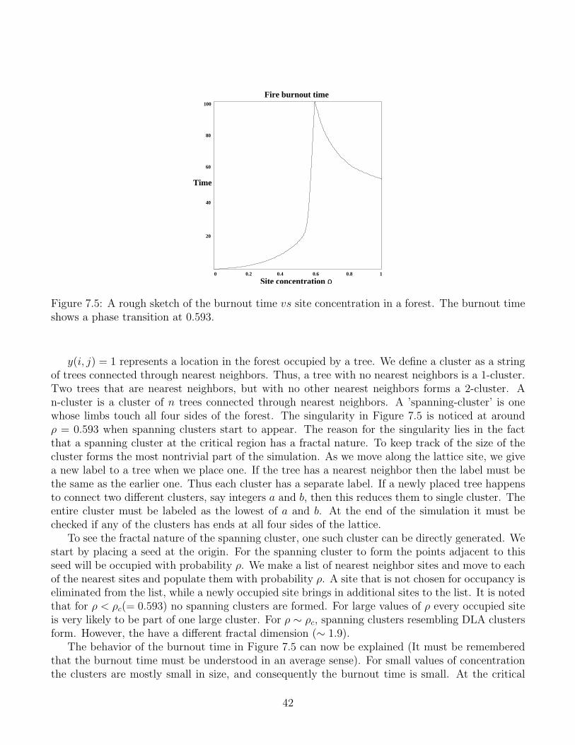
Percolation refers to the filtering or seeping of fluid through a porous medium - water through soil,oil through rock, etc.,. It also forms a good starting model for several other phenomena, such asdisease spreading or forest fires. We shall present the problem thus. Consider a forest of treesdistributed randomly with density ρ(0 < ρ < 1). Assume we set fire to one of trees at one end, andlet T be the time taken for the fire to die out. In a thin forest the fire dies down fast burning downa few trees, whereas for large ρ it can possibly burn down the whole forest. A rough plot T vs ρis shown in Figure 7.5. While the behavior is comprehensible for small and large values of ρ, thecurious aspect is the singular behavior at a certain value of ρ close to 0.6. Indeed the figure hintsa phase transition.

We simulate the forest of density ρ as follows: Construct of square grid of size N × N . Wegenerate a random sequence with uniform distribution 0 ≤ x < 1. At each site (i, j) we place a treeif the random number we pick from the sequence is less than ρ.

for i, j = 0, 1, ...N

pick random number x, 0 ≤ x < 1

y(i, j) = 1 if x < ρ, else y(i, j) = 0.

41

0 0.2 0.4 0.6 0.8 1

20

60

80

100

40

Time

Fire burnout time

Site concentration ρ

Figure 7.5: A rough sketch of the burnout time vs site concentration in a forest. The burnout timeshows a phase transition at 0.593.

y(i, j) = 1 represents a location in the forest occupied by a tree. We define a cluster as a stringof trees connected through nearest neighbors. Thus, a tree with no nearest neighbors is a 1-cluster.Two trees that are nearest neighbors, but with no other nearest neighbors forms a 2-cluster. An-cluster is a cluster of n trees connected through nearest neighbors. A ’spanning-cluster’ is onewhose limbs touch all four sides of the forest. The singularity in Figure 7.5 is noticed at aroundρ = 0.593 when spanning clusters start to appear. The reason for the singularity lies in the factthat a spanning cluster at the critical region has a fractal nature. To keep track of the size of thecluster forms the most nontrivial part of the simulation. As we move along the lattice site, we givea new label to a tree when we place one. If the tree has a nearest neighbor then the label must bethe same as the earlier one. Thus each cluster has a separate label. If a newly placed tree happensto connect two different clusters, say integers a and b, then this reduces them to single cluster. Theentire cluster must be labeled as the lowest of a and b. At the end of the simulation it must bechecked if any of the clusters has ends at all four sides of the lattice.

To see the fractal nature of the spanning cluster, one such cluster can be directly generated. Westart by placing a seed at the origin. For the spanning cluster to form the points adjacent to thisseed will be occupied with probability ρ. We make a list of nearest neighbor sites and move to eachof the nearest sites and populate them with probability ρ. A site that is not chosen for occupancy iseliminated from the list, while a newly occupied site brings in additional sites to the list. It is notedthat for ρ < ρc(= 0.593) no spanning clusters are formed. For large values of ρ every occupied siteis very likely to be part of one large cluster. For ρ ∼ ρc, spanning clusters resembling DLA clustersform. However, the have a different fractal dimension (∼ 1.9).

The behavior of the burnout time in Figure 7.5 can now be explained (It must be rememberedthat the burnout time must be understood in an average sense). For small values of concentrationthe clusters are mostly small in size, and consequently the burnout time is small. At the critical

42

Figure 7.6: A family of Koch curves generated through recursion. The curves are, by construction,scale invariant, or self similar. (Picture taken from Wikipedia).

value of concentration, the cluster has a fractal structure. Consequently, the fire takes a lengthyand tedious path within the grid, and hence a long time. For large values of concentration each treehas almost all neighboring sites populated. This results in the fire spreading fast in all directions,burning down the forest faster than at criticality.

43

Chapter 8

Statistical Mechanics

Contemporary statistical mechanics concerns largely with the phases of matter. The questionscentered around how a measured property of a system be related to a gross property of a largenumber of subsystems. However, over the last few decades the agenda has widened to include severalbranches where the statistical methods are directly applicable. Some examples are evolutionarybiology, financial markets, game theory, neural networks and problems in biology such as proteinfolding and DNA denaturation. Simulations form the primary back bone in understanding theseproblems. In this chapter we discuss the primary method of Monte Carlo simulation as applied instudying phase transition in the Ising model - a simplified version of a ferro(anti-ferro) magnet.

8.1 The Ising Model

The model assumes the magnet to be a lattice of spins that interact only with their nearest neighbors.Further the spins can take only either of the two values ±1. The hamiltonian of the system is givenby

H = −J∑

<i,j>

SiSj, Si,j = ±i. (8.1)

J > 0(J < 0) for ferro(anti-ferro) magnets. The notation < i, j indicates that the sum is overnearest neighbors. The model is a simplified version of the Heisenberg model for a lattice of spinvectors given by

H = −1

2

∑

i,j

(J1SxiSxj + J2SyiSyj + J3SziSzj). (8.2)

When J3 >> J2, J1, the model approximates to the Ising model.

8.2 Mean field theory

A sketch of a lattice of spins in a square lattice in 2-D is shown in Figure 8.1. A specific configurationof the spins, such as the one in Figure 8.1 will be referred to as a microstate. The preference ofthe system is for all the spins to be parallely aligned, as this is energetically favored. However,

44

Figure 8.1: The Ising model consists of ’up’ or ’down’ spins at each lattice site. The figure showsone possible microstate of the system. At thermal equilibrium with temperature T , the systemflip-flops through several microstates, with probability Pi proportionate to the Boltzmann factorexp(−Ei/kT ), where Ei is the energy of the microstate.

as the temperature of the system is increased the scenario changes. If the system is at thermalequilibrium at temperature T , i.e., it is in contact with a heat bath at T , the state of the systemgoes through several microstates as time progresses. The probability of the system being in aparticular microstate i of energy Ei is given by the Boltzmann factor

Pi ∝ e−Ei/kT . (8.3)

Over a time period the system at temperature T goes through several microstates. The measuredvalue of a physical quantity, say magnetization M is then the time average over these microstates.Since the ergodic hypothesis guarantees the equivalence of ensemble average and time average, wehave

M =∑

i

PiMi, (8.4)

where Mi is the value of magnetization in the microstate i.To see how magnetization changes as a function of temperature we shall first consider a param-

agnet in the presence of a magnetic field B, whose hamiltonian is given by

H = −µ∑

i

BSi. (8.5)

The probability of each spin being aligned along (or opposite to) B is

P+(−) =e+(−)µB/kT

eµB/kT + e−µB/kT. (8.6)

Thus average magnetization of the i’th spin is given by

< Si >= P+ − P−

= tanh(µB/kT ). (8.7)

45

We rewrite the Ising hamiltonian Eq. (8.1) as

H = −(J∑

<i,j>

Sj)Si = −∑

i

BeffSi, (8.8)

i.e., we assume the ith spin to be acted upon by the mean field due to its neighboring spins. Nowwe make the (mean field) approximation that for a large system the average behavior of ith spin isas good as any other. I.e.,

< Si >=< Sj >=< S > . (8.9)

Substituting these results in that of the paramagnet we have

< S >= tanh(Jz < S > /kT ), (8.10)

where z is the number of nearest neighbors. In a n-D square lattice z = 2n. Approximatingtanh(x) = x − x3/3 we get

< S >=zJ < S >

kT− 1

3(zJ < S >

kT)3 (8.11)

with solutions < S >= 0 and

< S >=

√

3

T(kT

zJ)3(

zJ

k− T )1/2 ∼ (Tc − T )β (8.12)

where β = 1/2 is a critical coefficient. The second solution implies that a T < Tc the magnetization< S > has a nonzero value, thus showing a phase transition.

8.3 Newton’s method

Equation (8.10) is a transcendental equation. If we define

f(x) = x − tanh(ax), (8.13)

solving Eq. (8.10) is equivalent to finding x0 such that f(x0) = 0. To do this (or solve any algebraicequation) we employ the Newton’s method. Let x0 be solution we seek. We start with a seedsolution x1. If x0 = x1 + ∆x1 then,

f(x0) = f(x1 + ∆x1) = f(x1) + fx(x1)∆x1 (8.14)

Since f(x0) = 0, this implies

∆x1 = − f(x1)

fx(x1). (8.15)

Using ∆x1 we find a new value for the seed, x2 = x1 + ∆x1. The solution is obtained by repeatingthis iteration till a tolerance level is reached.

46

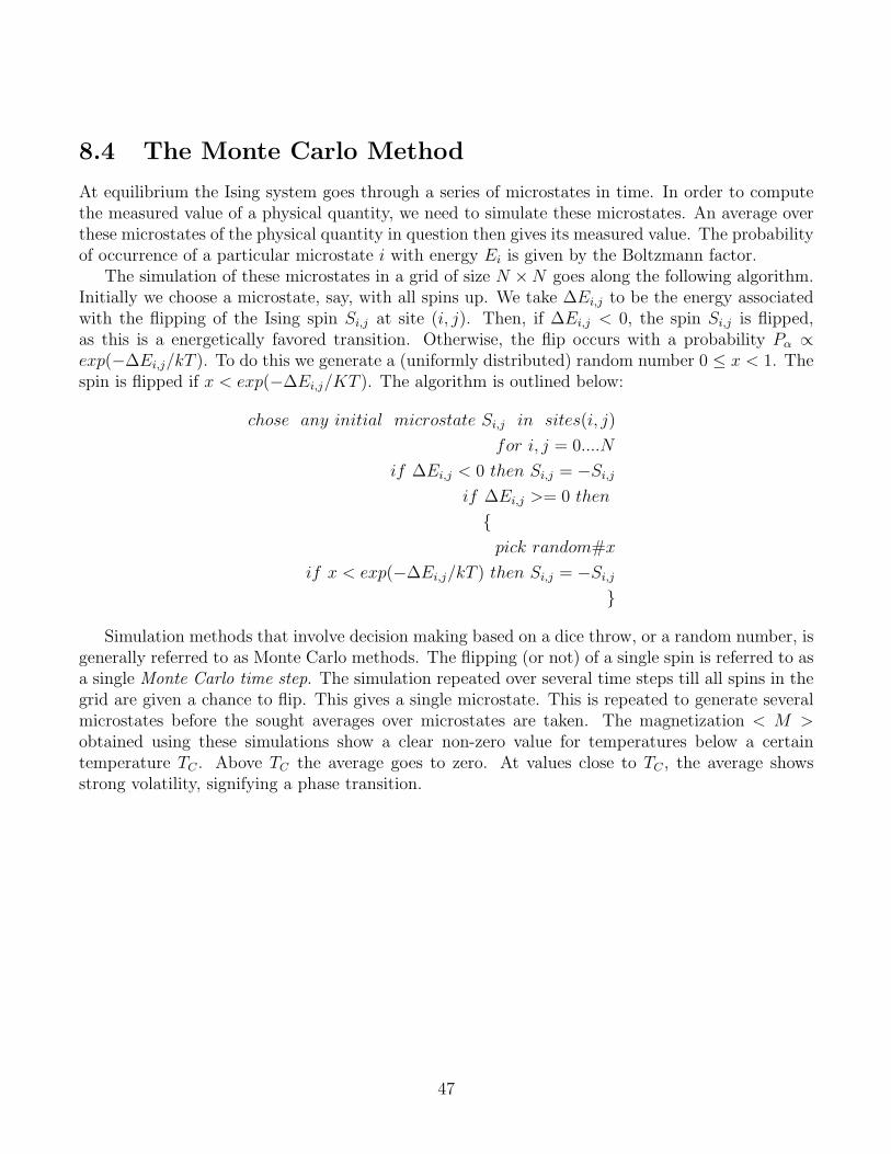
8.4 The Monte Carlo Method

At equilibrium the Ising system goes through a series of microstates in time. In order to computethe measured value of a physical quantity, we need to simulate these microstates. An average overthese microstates of the physical quantity in question then gives its measured value. The probabilityof occurrence of a particular microstate i with energy Ei is given by the Boltzmann factor.

The simulation of these microstates in a grid of size N ×N goes along the following algorithm.Initially we choose a microstate, say, with all spins up. We take ∆Ei,j to be the energy associatedwith the flipping of the Ising spin Si,j at site (i, j). Then, if ∆Ei,j < 0, the spin Si,j is flipped,as this is a energetically favored transition. Otherwise, the flip occurs with a probability Pα ∝exp(−∆Ei,j/kT ). To do this we generate a (uniformly distributed) random number 0 ≤ x < 1. Thespin is flipped if x < exp(−∆Ei,j/KT ). The algorithm is outlined below:

chose any initial microstate Si,j in sites(i, j)

for i, j = 0....N

if ∆Ei,j < 0 then Si,j = −Si,j

if ∆Ei,j >= 0 then

pick random#x

if x < exp(−∆Ei,j/kT ) then Si,j = −Si,j

Simulation methods that involve decision making based on a dice throw, or a random number, isgenerally referred to as Monte Carlo methods. The flipping (or not) of a single spin is referred to asa single Monte Carlo time step. The simulation repeated over several time steps till all spins in thegrid are given a chance to flip. This gives a single microstate. This is repeated to generate severalmicrostates before the sought averages over microstates are taken. The magnetization < M >obtained using these simulations show a clear non-zero value for temperatures below a certaintemperature TC . Above TC the average goes to zero. At values close to TC , the average showsstrong volatility, signifying a phase transition.

47