*Under revision

LECTURE NOTE

COURSE CODE- BCE 305

TRANSPORTATION ENGINEERING-I

*Under revision

SYLLABUS

Module-I

Transportation by roads, railways, water ways & air ways – their importance& limitation.

Road development & planning in India. Financing, Highway alignment & engineering

surveys for highway location.

Geometric design-Cross section elements, Design speed, sight distance, super elevation,

horizontal & vertical alignment including curves.

Module-II

Traffic Engineering – Traffic studies & their importance.

Highway materials – Their properties & tests, selection, requirements of bituminous mixes,

marshall test.

Earthwork – measurement & rates, setting out of earth work, computation of areas &

volumes-Prismoidal & Trapezoidal methods.

Module-III

Pavement design-Use of CBR method for design of flexible pavement, IRC recommendation

for design of rigid pavement.

Highway drainage, pavement failure, Evaluation, Maintenance & Strengthening of existing

pavement.

Module-IV

Classification of bridges, Consideration of location of bridge site, Investigation & data

collection, Calculation of run off under bridge, Determination of water way, Choice of bridge

span-economic span, Determination of maximum scour depth.

Bridge Superstructure-types, suitability.

Bridge foundation-Types, Sinking of well.

Books for Reference:

(1) Highway Engineering-By Khanna & Justo (Nemchand & Bros., Roorkee (U.A))

(2) Perniciples & Practice of Highway Engineering – By Dr. L.R. Kadiyalli (Khanna

publisher)

(3) Bridge Engineering – By S.P. Bindra (Dhanpat Rai publication)

(4) Bridge Engineering-By D.J. Victor

*Under revision

ACKNOWLEDGEMENT

We would like to acknowledge various sources from which the lecture

note was prepared. Especially we would like to mention that the lecture

note has been prepared in the light of material available with NPTEL,

Transportation-I prepared by Prof. Tom V. Mathew and Prof. K.V.

Krishna Rao of IIT Bombay.

*Under revision

Lecture-1

INTRODUCTION

1.1 Overview From the beginning of history, human sensitivity has revealed an urge for mobility leading to a

measure of Society's progress. The history of this mobility or transport is the history of

civilization. For any country to develop with right momentum modern and efficient Transport as

a basic infrastructure is a must. Transport (British English) or transportation (American

English) is the movement of people and goods from one place to another. The term is derived

from the Latin trans ("across") and portare ("to carry").

1.2 Means of Transport

Fig.1.1 Means of Transport

1.3. Advantage and Disadvantage Different Modes of Transport

(A) Road Transport

Advantages Disadvantages

1. Less Capital Outlay

2. Door to Door Service

3. Service in Rural Areas

4. Flexible Service

5. Suitable for Short Distance

6. Lesser Risk of Damage in Transit

7. Saving in Packing Cost

8. Rapid Speed

9. Less Cost

1. Seasonal Nature

2. Accidents and Breakdowns

3. Unsuitable for Long Distance and Bulky

Traffic

4. Slow Speed

5. Lack of Organisation

*Under revision

10. Private Owned Vehicles

11. Feeder to other Modes of Transport

(B) Railway Transport

Advantages Disadvantages

1. Dependable

2. Better Organised

3. High Speed over Long Distances

4. Suitable for Bulky and Heavy Goods

5. Cheaper Transport

6. Safety

7. Larger Capacity

8. Public Welfare

9. Administrative Facilities of Government

10. Employment Opportunities

1. Huge Capital Outlay

2. Lack of Flexibility

3. Lack of Door to Door Service

4. Monopoly

5. Unsuitable for Short Distance and Small

Loads

6. Booking Formalities

7. No Rural Service

8. Under-utilised Capacity

9. Centralised Administration

(C) Air Transport Advantages Disadvantages

1. High Speed

2. Comfortable and Quick Services

3. No Investment in Construction of Track

4. No Physical Barriers

5. Easy Access

6. Emergency Services

7. Quick Clearance

8. Most Suitable for Carrying Light Goods of

High Value

9. National Defence

10. Space Exploration

1. Very Costly

2. Small Carrying Capacity

3. Uncertain and Unreliable

4. Breakdowns and Accidents

5. Large Investment

6. Specialised Skill

7. Unsuitable for Cheap and Bulky Goods

8. Legal Restrictions

1.4. Elements of transport

The movement of goods or passenger traffic, through rail, sea, air or road transport requires

adequate infrastructure facilities for the free flow from the place of origin to the place of

destination. Irrespective of modes, every transport system has some common elements:

a) Vehicle or carrier to carry passenger or goods

b) Route or path for movement of carriers

c) Terminal facilities for loading and unloading of goods and passengers from carriers

d) Prime Mover

e) Transit time and cost

f) Cargo

*Under revision

These elements influence the effectiveness of different modes of transport and their utility to

users.

• Vehicles: The dimension of vehicles, its capacity and type are some of the factors, which

influence the selection of a transport system for movement of goods from one place to the other.

• Routes: Routes play an important role in movement of carriers from one point to another point.

It may be surface roads, navigable waterways and roadways. Availability of well-designed and

planned routes without any obstacle for movement of transport vehicles in specific routes, is a

vital necessity for smooth flow of traffic.

• Terminal Facilities: - The objective of transportation cant be fulfilled unless proper facilities

are available for loading and unloading of goods or entry and exit of passengers from carrier.

Terminal facilities are to be provided for loading and unloading of trucks, wagons etc on a

continuous basis.

• Prime Mover: - The power utilized for moving of vehicles for transportation of cargo from

one place to another is another important aspect of the total movement system.

• Transit time and cost: - Transportation involve time and cost. The time element is a valid

factor for determining the effectiveness of a particular mode of transport. The transit time of

available system of transportation largely determines production and consumption pattern of

perishable goods in an economy.

• Cargo: - Transportation basically involves movement of cargo from one place to another.

Hence, nature and size of cargo constitute the basis of any goods transport system.

1.4 Major disciplines of transportation Transportation engineering can be broadly consisting of the four major parts:

1. Transportation Planning

2. Geometric Design

3. Pavement Design

4. Traffic Engineering

*Under revision

Lecture 2

HIGHWAY DEVELOPMENT IN INDIA

2.1 Overview

Road network provides the arterial network to facilitate trade, transport, social integration and

economic development. It facilitates specialization, extension of markets and exploitation of

economies of scale. It is used for the smooth conveyance of both people and goods.

Transportation by road has the advantage over other means of transport because of its easy

accessibility, flexibility of operations, door-to-door service and reliability. Consequently,

passenger and freight movement in India over the years have increasingly shifted towards roads

vis-à-vis other means of transport.

2.2 History of highway engineering The history of highway engineering gives us an idea about the roads of ancient times. Roads in

Rome were constructed in a large scale and it radiated in many directions helping them in

military operations. Thus they are considered to be pioneers in road construction. In this section

we will see in detail about Ancient roads, Roman roads, British roads, French roads etc.

2.2.1 Ancient Roads

The most primitive mode of transport was by foot. These human pathways would have been

developed for specific purposes leading to camp sites, food, streams for drinking water etc. The

invention of wheel in Mesopotamian civilization led to the development of animal drawn

vehicles. To provide adequate strength to carry the wheels, the new ways tended to follow the

sunny drier side of a path. After the invention of wheel, animal drawn vehicles were developed

and the need for hard surface road emerged. Traces of such hard roads were obtained from

various ancient civilization dated as old as 3500 BC. The earliest authentic record of road was

found from Assyrian empire constructed about 1900 BC.

2.2.2 Roman roads

The earliest large scale road construction is attributed to Romans who constructed an extensive

system of roads radiating in many directions from Rome. Romans recognized that the

fundamentals of good road construction were to provide good drainage, good material and good

workmanship. Their roads were very durable, and some still exist. The roads were bordered on

both sides by longitudinal drains. A typical corss section is shown in Fig.2.1. This was a raised

formation up to a 1 meter high and 15 m wide and was constructed with materials excavated

during the side drain construction. This was then topped with a sand leveling course. In the case

of heavy traffic, a surface course of large 250 mm thick hexagonal ag stones were provided They

*Under revision

mixed lime and volcanic puzzolana to make mortar and they added gravel to this mortar to make

concrete. Thus concrete was a major Roman road making innovation.

Fig.2.1 Roman roads

2.2.3 French roads The significant contributions were given by Tresaguet in 1764 and a typical cross section of this

road is given in Figure 2.2. He developed a cheaper method of construction than the lavish and

locally unsuccessful revival of Roman practice. The pavement used 200 mm pieces of quarried

stone of a more compact form and shaped such that they had at least one at side which was

placed on a compact formation. Smaller pieces of broken stones were then compacted into the

spaces between larger stones to provide a level surface. Finally the running layer was made with

a layer of 25 mm sized broken stone. All this structure was placed in a trench in order to keep the

running surface level with the surrounding country side. This created major drainage problems

which were counteracted by making the surface as impervious as possible, cambering the surface

and providing deep side ditches.

Fig. 2.2. French roads

2.2.4 British roads The British government also gave importance to road construction. The British engineer John

*Under revision

Macadam introduced what can be considered as the first scientific road construction method.

Stone size was an important element of Macadam recipe. By empirical observation of many

roads, he came to realize that 250 mm layers of well compacted broken angular stone would

provide the same strength a better running surface than an expensive pavement founded on large

stone blocks. Thus he introduced an economical method of road construction. A typical cross

section of British roads is given in Fig. 2.3.

Fig. 2.3. British roads

2.2.5 Modern roads

The modern roads by and large follow Macadam's construction method. Use of bituminous

concrete and cement concrete are the most important developments. Development of new

equipments helps in the faster construction of roads. Many easily and locally available materials

are tested in the laboratories and then implemented on roads for making economical and durable

pavements.

2.3. Road Development in India

Excavations in the sites of Indus valley revealed the existence of planned roads in India as old as

2500-3500 BC. The Mauryan kings also built very good roads. During the time of Mughal

period, roads in India were greatly improved. Roads linking North-West and the Eastern areas

through gangetic plains were built during this time. The construction of Grand-Trunk road

connecting North and South is a major contribution of the British.

2.3.1 Modern developments The First World War period and that immediately following it found a rapid growth in motor

transport. So need for better roads became a necessity. For that, the Government of India

appointed a committee called Road development Committee with Mr.M.R. Jayakar as the

chairman. This committee came to be known as Jayakar committee.

*Under revision

Jayakar Committee In 1927 Jayakar committee for Indian road development was appointed. The major

recommendations and the resulting implementations were:

Committee found that the road development of the country has become beyond the

capacity of local governments and suggested that Central government should take

the proper charge considering it as a matter of national interest.

They gave more stress on long term planning programme, for a period of 20 years

(hence called twenty year plan) that is to formulate plans and implement those plans

with in the next 20 years.

One of the recommendations was the holding of periodic road conferences to

discuss about road construction and development. This paved the way for the

establishment of a semi-official technical body called Indian Road Congress (IRC)

in 1934

The committee suggested imposition of additional taxation on motor transport

which includes duty on motor spirit, vehicle taxation, license fees for vehicles

plying for hire. This led to the introduction of a development fund called Central

road fund in 1929. This fund was intended for road development.

The committee suggested imposition of additional taxation on motor transport

which includes duty on motor spirit, vehicle taxation, and license fees for vehicles

plying for hire. This led to the introduction of a development fund called Central

road fund in 1929. This fund was intended for road development.

Nagpur road congress 1943

A twenty year development programme for the period (1943-1963) was finalized. It was the first

attempt to prepare a co-ordinated road development programme in a planned manner. The roads were divided into four classes:

National highways which would pass through states, and places having national

importance for strategic, administrative and other purposes. State highways which would be the other main roads of a state.

District roads which would take traffic from the main roads to the interior of the district.

According to the importance, some are considered as major district roads and the

remaining as other district roads. Village roads which would link the villages to the road system.

The committee planned to construct 2 lakh kms of road across the country within 20 years. They

*Under revision

recommended the construction of star and grid pattern of roads throughout the country. One of

the objective was that the road length should be increased so as to give a road density of 16kms

per 100 sq.km

Bombay road congress 1961 The length of roads envisaged under the Nagpur plan was achieved by the end of it, but the road

system was deficient in many respects. Accordingly a 20-year plan was drafted by the Roads

wing of Government of India, which is popularly known as the Bombay plan. The highlights of

the plan were: It was the second 20 year road plan (1961-1981)

The total road length targeted to construct was about 10 lakhs.

Rural roads were given specific attention.

They suggested that the length of the road should be increased so as to give a road

density of 32kms/100 sq.km The construction of 1600 km of expressways was also then included in the plan.

Lucknow road congress 1984 Some of the salient features of this plan are as given below: This was the third 20 year road plan (1981-2001). It is also called Lucknow road plan.

It aimed at constructing a road length of 12 lakh kilometers by the year 1981 resulting in

a road density of 82kms/100 sq.km The plan has set the target length of NH to be completed by the end of seventh, eighth

and ninth five year plan periods. It aims at improving the transportation facilities in villages, towns etc. such that no part

of country is farther than 50 km from NH. One of the goals contained in the plan was that expressways should be constructed on

major traffic corridors to provide speedy travel. Energy conservation, environmental quality of roads and road safety measures were also

given due importance in this plan.

2.4 Current Scenario

About 60 per cent of freight and 87 per cent passenger traffic is carried by road. Although

National Highways constitute only about 2 per cent of the road network, it carries 40 per cent of

*Under revision

the total road traffic. Easy availability, adaptability to individual needs and cost savings are some

of the factors which go in favour of road transport. Road transport also acts as a feeder service to

railway, shipping and air traffic. The number of vehicles has been growing at an average pace of

around 10 per cent per annum. The share of road traffic in total traffic has grown from 13.8 per

cent of freight traffic and 15.4 per cent of passenger traffic in 1950-51 to an estimated 62.9 per

cent of freight traffic and 90.2 per cent of passenger traffic by the end of 2009-10. The rapid

expansion and strengthening of the road network, therefore, is imperative, to provide for both

present and future traffic and for improved accessibility to the hinterland.

*Under revision

Lecture 3

HIGHWAY PLANNING

2.1 Overview

Highway design is only one element in the overall highway development process. Historically,

detailed design occurs in the middle of the process, linking the preceding phases of planning and

project development with the subsequent phases of right-of-way acquisition, construction, and

maintenance. It is during the first three stages, planning, project development, and design, that

designers and communities, working together, can have the greatest impact on the final design

features of the project. In fact, the flexibility available for highway design during the detailed

design phase is limited a great deal by the decisions made at the earlier stages of planning and

project development.

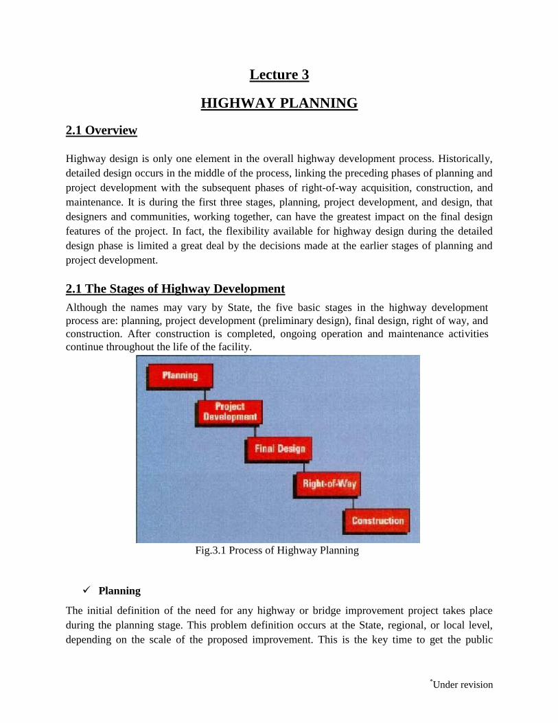
2.1 The Stages of Highway Development Although the names may vary by State, the five basic stages in the highway development

process are: planning, project development (preliminary design), final design, right of way, and

construction. After construction is completed, ongoing operation and maintenance activities

continue throughout the life of the facility.

Fig.3.1 Process of Highway Planning

Planning

The initial definition of the need for any highway or bridge improvement project takes place

during the planning stage. This problem definition occurs at the State, regional, or local level,

depending on the scale of the proposed improvement. This is the key time to get the public

*Under revision

involved and provide input into the decision making process. The problems identified usually fall

into one or more of the following four categories:

1. The existing physical structure needs major repair/replacement (structure repair).

2. Existing or projected future travel demands exceed available capacity, and access to

transportation and mobility need to be increased (capacity).

3. The route is experiencing an inordinate number of safety and accident problems that can

only be resolved through physical, geometric changes (safety).

4. Developmental pressures along the route make a reexamination of the number, location,

and physical design of access points necessary (access).

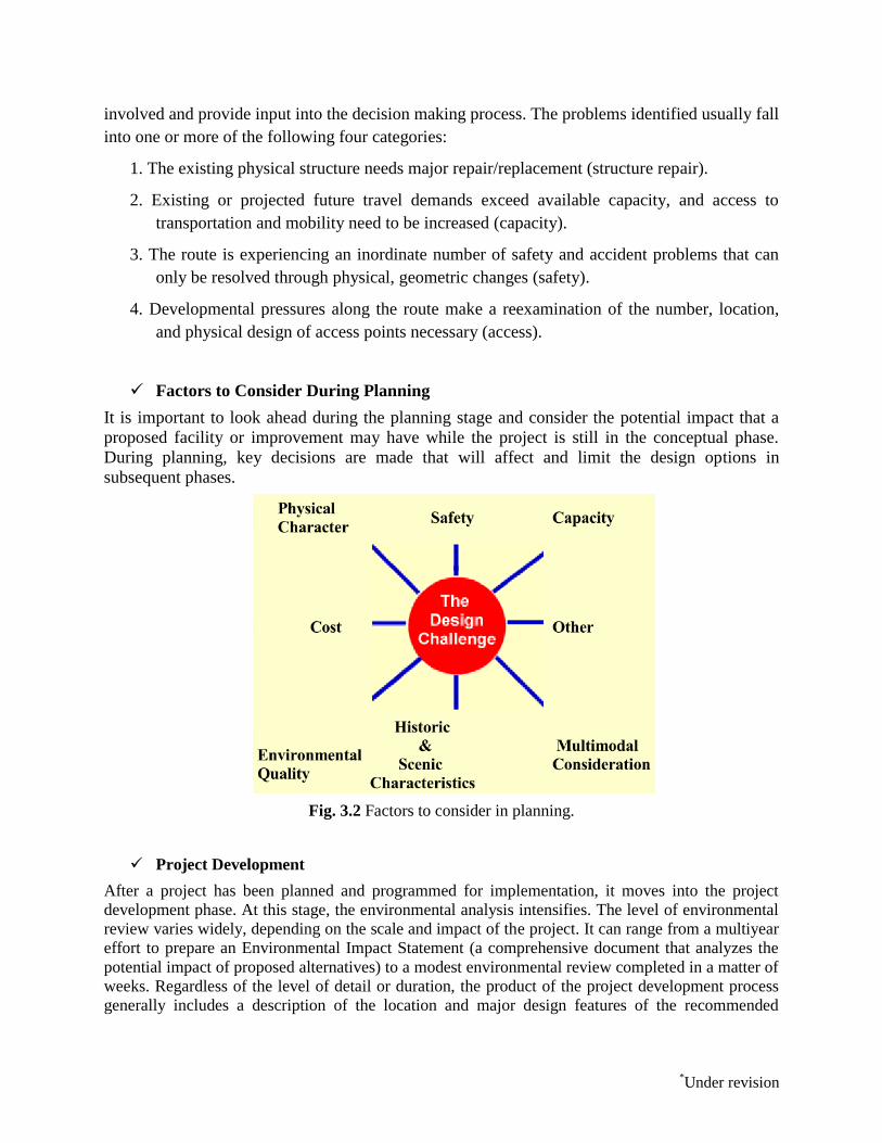
Factors to Consider During Planning

It is important to look ahead during the planning stage and consider the potential impact that a

proposed facility or improvement may have while the project is still in the conceptual phase.

During planning, key decisions are made that will affect and limit the design options in

subsequent phases.

Fig. 3.2 Factors to consider in planning.

Project Development

After a project has been planned and programmed for implementation, it moves into the project

development phase. At this stage, the environmental analysis intensifies. The level of environmental

review varies widely, depending on the scale and impact of the project. It can range from a multiyear

effort to prepare an Environmental Impact Statement (a comprehensive document that analyzes the

potential impact of proposed alternatives) to a modest environmental review completed in a matter of

weeks. Regardless of the level of detail or duration, the product of the project development process

generally includes a description of the location and major design features of the recommended

*Under revision

project that is to be further designed and constructed, while continually trying to avoid, minimize, and mitigate environmental impact.

Final Design

After a preferred alternative has been selected and the project description agreed upon as stated

in the environmental document, a project can move into the final design stage. The product of

this stage is a complete set of plans, specifications, and estimates (PS&Es) of required

quantities of materials ready for the solicitation of construction bids and subsequent

construction. Depending on the scale and complexity of the project, the final design process

may take from a few months to several years. The following paragraphs discuss some important considerations of design, including:

• Developing a concept

• Considering scale and

• Detailing the design.

Developing a Concept

A design concept gives the project a focus and helps to move it toward a specific direction.

There are many elements in a highway, and each involves a number of separate but interrelated

design decisions. Integrating all these elements to achieve a common goal or concept helps the

designer in making design decisions. Some of the many elements of highway design are

a. Number and width of travel lanes, median type and width, and shoulders

b. Traffic barriers

c. Overpasses/bridges

d. Horizontal and vertical alignment and affiliated landscape.

Considering Scale

People driving in a car see the world at a much different scale than people walking on the

street. This large discrepancy in the design scale for a car versus the design scale for people

has changed the overall planning of our communities. For example, it has become common

in many suburban commercial areas that a shopper must get in the car and drive from one

store to the next. The design element with the greatest effect on the scale of the roadway is its width, or cross

section. The cross section can include a clear zone, shoulder, parking lanes, travel lanes,

and/or median. The wider the overall roadway, the larger its scale; however, there are some

design techniques that can help to reduce the perceived width and, thus, the perceived scale

of the roadway. Limiting the width of pavement or breaking up the pavement is one option.

*Under revision

In some instances, four lane roadways may look less imposing by designing a grass or

planted median in the center.

Detailing the Design

Particularly during the final design phase, it is the details associated with the project that are

important. Employing a multidisciplinary design team ensures that important design details

are considered and those they are compatible with community values. Often it is the details

of the project that are most recognizable to the public. A multidisciplinary design team can

produce an aesthetic and functional product when the members work together and are

flexible in applying guidelines.

Right-of-way, Construction, And Maintenance Once the final designs have been prepared and needed right-of-way is purchased,

construction bid packages are made available, a contractor is selected, and construction is

initiated. During the right-of-way acquisition and construction stages, minor adjustments in

the design may be necessary; therefore, there should be continuous involvement of the

design team throughout these stages. Construction may be simple or complex and may

require a few months to several years. Once construction has been completed, the facility is

ready to begin its normal sequence of operations and maintenance. Even after the completion of construction, the character of a road can be changed by

inappropriate maintenance actions. For example, the replacement of sections of guardrail

damaged or destroyed in crashes commonly utilizes whatever spare guardrail sections may be

available to the local highway maintenance personnel at the time.

Stages of Highway Development Summaries of the five basic stages in highway planning and development.

Stages Description of Activity Planning Identification of transportation needs and program project to be built

Within financial constraints.

Project Development The transportation project is more clearly defined. Alternative locations

and design features are developed and an alternative is selected.

Design The design team develops detailed design and specification.

Right-of-way Land needed for the project is acquired.

construction Selection of contractor, who then builds the project.

2.3 Highway Route Surveys and Location

To determine the geometric features of road design, the following surveys must be

conducted after the necessity of the road is decided.

*Under revision

A variety of survey and investigations have to be carried out by Road engineers and

multidiscipline persons.

A. Transport Planning Surveys o Traffic Surveys o Highway inventories o Pavement Deterioration Study o Accident study

B. Alignment and Route location surveys Desk study Reconnaissance

Preliminary Survey Final location survey

C. Drainage Studies o Surface run- off : Hydrologic and hydraulic o Subsurface drainage: Ground water & Seepage o Cross–drainage: Location and waterway area required for

the cross-drainage structures. D. Soil Survey

Desk study

Site Reconnaissance E. Pavement Design investigation Soil property and strength, Material Survey

*Under revision

Lecture 4

INTRODUCTION TO GEOMETRIC DESIGN

4.1. Overview Geometric design for transportation facilities includes the design of geometric cross sections,

horizontal alignment, vertical alignment, intersections, and various design details. These basic

elements are common to all linear facilities, such as roadways, railways, and airport runways and

taxiways. Although the details of design standards vary with the mode and the class of facility,

most of the issues involved in geometric design are similar for all modes. In all cases, the goals

of geometric design are to maximize the comfort, safety, and economy of facilities, while

minimizing their environ-mental impacts. This chapter focuses on the fundamentals of geometric

design, and presents standards and examples from different modes.

The geometric design of highways deals with the dimensions and layout of visible features of the

highway. The features normally considered are the cross section elements, sight distance

consideration, horizontal curvature, gradients, and intersection. The design of these features is to

a great extend influenced by driver behavior and psychology, vehicle characteristics, traffic

characteristics such as speed and volume. Proper geometric design will help in the reduction of

accidents and their severity. Therefore, the objective of geometric design is to provide optimum

efficiency in traffic operation and maximum safety at reasonable cost.

The planning cannot be done stage wise like that of a pavement, but has to be done well in

advance. The main components that will be discussed are:

1. Factors affecting the geometric design,

2. Highway alignment, road classification,

3. Pavement surface characteristics,

4. Cross-section elements including cross slope, various widths of roads and features in the

road margins.

5. Sight distance elements including cross slope, various widths and features in the road

margins.

6. Horizontal alignment which includes features like super elevation, transition curve, extra

widening and set back distance.

7. Vertical alignment and its components like gradient, sight distance and design of length of

curves.

8. Intersection features like layout, capacity, etc.

*Under revision

4.2 Factors affecting geometric design

Design speed: Design speed is the single most important factor that affects the

geometric design. It directly affects the sight distance, horizontal curve, and the length

of vertical curves. Since the speed of vehicles vary with driver, terrain etc, a design

speed is adopted for all the geometric design.

Topography: It is easier to construct roads with required standards for a plain terrain.

However, for a given design speed, the construction cost increases multi form with the

gradient and the terrain.

Traffic factors: It is of crucial importance in highway design, is the traffic data both

current and future estimates. Traffic volume indicates the level of services (LOS) for

which the highway is being planned and directly affects the geometric features such as

width, alignment, grades etc., without traffic data it is very difficult to design any

highway

Design Hourly Volume and Capacity: The general unit for measuring traffic on

highway is the Annual Average Daily Traffic volume, abbreviated as AADT. The

traffic flow (or) volume keeps fluctuating with time, from a low value during off peak

hours to the highest value during the peak hour. It will be uneconomical to design the

roadway facilities for the peak traffic flow.

Environmental and other factors: - The environmental factors like air pollution,

noise pollution, landscaping, aesthetics and other global conditions should be given due

considerations in the geometric design of roads.

4.3 Road classification

The roads can be classified in many ways. The classification based on speed and accessibility is

the most generic one. Note that as the accessibility of road increases, the speed reduces. (See

Fig. 4.1). Accordingly, the roads can classified as follows in the order of increased accessibility

and reduced speeds.

Freeways: Freeways are access controlled divided highways. Most freeways are four

lanes, two lanes each direction, but many freeways widen to incorporate more lanes as

they enter urban areas. Access is controlled through the use of interchanges, and the type

*Under revision

of interchange depends upon the kind of intersecting road way (rural roads, another

freeway etc.)

Expressways: They are superior type of highways and are designed for high speeds(120

km/hr is common), high traffic volume and safety. They are generally provided with

grade separations at intersections. Parking, loading and unloading of goods and

pedestrian traffic is not allowed on expressways.

Highways: They represent the superior type of roads in the country. Highways are of two

types - rural highways and urban highways. Rural highways are those passing through

rural areas (villages) and urban highways are those passing through large cities and

towns, i.e. urban areas.

Arterials: It is a general term denoting a street primarily meant for through traffic

usually on a continuous route. They are generally divided highways with fully or

partially controlled access. Parking, loading and unloading activities are usually

restricted and regulated. Pedestrians are allowed to cross only at intersections/designated

pedestrian crossings.

Local streets: A local street is the one which is primarily intended for access to

residence, business or abutting property. It does not normally carry large volume of

traffic and also it allows unrestricted parking and pedestrian movements.

Collectors streets: These are streets intended for collecting and distributing traffic to and

from local streets and also for providing access to arterial streets. Normally full access is

provided on these streets. There are few parking restrictions except during peak hours.

Fig.4.1. Speed vs accessibility

*Under revision

Roads can be classified based on some other criteria. They are given in detail below.

Based on usage This classified is based on whether the roads can be used during di erent seasons of the year.

All-weather roads: Those roads which are negotiable during all weathers, except at

major river crossings where interruption of tra c is permissible up to a certain extent

are called all weather roads.

Fair-weather roads: Roads which are negotiable only during fair weather are called

fair weather roads.

Based on carriage way This classification is based on the type of the carriage way or the road pavement.

Paved roads with hard surface : If they are provided with a hard pavement course

such roads are called paved roads.(eg: stones, Water bound macadam (WBM),

Bituminous macadam (BM), concrete roads)

Unpaved roads: Roads which are not provided with a hard course of atleast a WBM

layer they is called unpaved roads. Thus earth and gravel roads come under this

category.

Based on pavement surface Based on the type of pavement surfacing provided, they are classified as surfaced and unsurfaced

roads.

Surfaced roads (BM, concrete): Roads which are provided with a bituminous or

cement concreting surface are called surfaced roads.

Unsurfaced roads (soil/gravel): Roads which are not provided with a bituminous or

cement concreting surface are called unsurfaced roads.

Other criteria Roads may also be classified based on the traffic volume in that road, load transported through

that road, or location and function of that road.

Traffic volume: Based on the traffic volume, they are classified as heavy, medium

and light tra c roads. These terms are relative and so the limits under each class may

be expressed as vehicles per day.

Load transported: Based on the load carried by these roads, they can be classified as

class I, class II, etc. or class A, class B etc. and the limits may be expressed as

tonnes per day.

*Under revision

Location and function: The classification based on location and function should be a

more acceptable classification since they may be defined clearly.

4.3 Highway alignment Once the necessity of the highway is assessed, the next process is deciding the alignment. The highway

alignment can be either horizontal or vertical and they are described in detail in the following

sections.

4.3.1 Alignment

The position or the layout of the central line of the highway on the ground is called the

alignment. Horizontal alignment includes straight and curved paths. Vertical alignment includes

level and gradients. Alignment decision is important because a bad alignment will enhance the

construction, maintenance and vehicle operating cost. Once an alignment is xed and constructed,

it is not easy to change it due to increase in cost of adjoining land and construction of costly

structures by the roadside.

4.3.2 Requirements

The requirements of an ideal alignment are: The alignment between two terminal stations should be short and as far as possible be

straight, but due to some practical considerations deviations may be needed.

The alignment should be easy to construct and maintain. It should be easy for the

operation of vehicles. So to the maximum extend easy gradients and curves should be

provided.

It should be safe both from the construction and operating point of view especially at

slopes, embankments, and cutting. It should have safe geometric features.

The alignment should be economical and it can be considered so only when the initial

cost, maintenance cost, and operating cost is minimum.

4.3.3. Factors controlling alignment We have seen the requirements of an alignment. But it is not always possible to satisfy all these

requirements. Hence we have to make a judicial choice considering all the factors. The various factors that control the alignment are as follows:

Obligatory points: These are the control points governing the highway alignment.

These points are classified into two categories. Points through which it should pass

and points through which it should not pass. Some of the examples are:

Bridge site: The bridge can be located only where the river has straight and

permanent path and also where the abutment and pier can be strongly founded. The

road approach to the bridge should not be curved and skew crossing should be

avoided as possible. Thus to locate a bridge the highway alignment may be changed.

*Under revision

Mountain: While the alignment passes through a mountain, the various alternatives

are to either construct a tunnel or to go round the hills. The suitability of the

alternative depends on factors like topography, site conditions and construction and

operation cost.

Intermediate town: The alignment may be slightly deviated to connect an

intermediate town or village nearby. These were some of the obligatory points through which the alignment should pass. Coming to

the second category that is the points through which the alignment should not pass are:

Religious places: These have been protected by the law from being acquired for any

purpose. Therefore, these points should be avoided while aligning.

Very costly structures: Acquiring such structures means heavy compensation which

would result in an increase in initial cost. So the alignment may be deviated not to pass

through that point.

Lakes/ponds etc: The presence of a lake or pond on the alignment path would also

necessitate deviation of the alignment.

Traffic: The alignment should suit the traffic requirements. Based on the origin-

destination data of the area, the desire lines should be drawn. The new alignment should

be drawn keeping in view the desire lines, traffic flow pattern etc.

Geometric design: Geometric design factors such as gradient, radius of curve, sight

distance etc. also governs the alignment of the highway. To keep the radius of curve

minimum, it may be required to change the alignment of the highway. The alignments

should be finalized such that the obstructions to visibility do not restrict the minimum

requirements of sight distance. The design standards vary with the class of road and the

terrain and accordingly the highway should be aligned.

*Under revision

Lecture 5

Cross sectional elements 5.1 Overview The primary consideration in the design of geometric cross sections for highways, run-ways, and taxiways is

drainage. Details vary depending on the type of facility Highway cross sections consist of traveled way, shoulders

(or parking lanes), and drainage channels. Shoulders are intended primarily as a safety feature. They provide for

accommodation of stopped vehicles, emergency use, and lateral support of the pavement. Shoulders may be either

paved or unpaved. Drainage channels may consist of ditches (usually grassed swales) or of paved shoulders with

berms or curbs and gut-ters. Cross section of various roads are given bellow.

Fig.5.1. Two-lane highway cross section, with ditches.

Fig.5.2.Divided highway cross section, depressed median, with ditches.

Pavement surface characteristics

For a safe and comfortable driving four aspects of the pavement surface are important; the

friction between the wheels and the pavement surface, smoothness of the road surface, the light

re ection characteristics of the top of pavement surface, and drainage to water.

*Under revision

Friction Friction between the wheel and the pavement surface is a crucial factor in the design of

horizontal curves and thus the safe operating speed. Further, it also a ect the acceleration and

deceleration ability of vehicles. Lack of adequate friction can cause skidding or slipping of

vehicles.

Skidding happens when the path traveled along the road surface is more than the

circumferential movement of the wheels due to friction

Slip occurs when the wheel revolves more than the corresponding longitudinal movement

along the road. Various factors that a ect friction are:

The frictional force that develops between the wheel and the pavement is the load acting

multiplied by a factor called the coe cient of friction and denoted as f . The choice of the value of

f is a very complicated issue since it depends on many variables. IRC suggests the coe cient of

longitudinal friction as 0.35-0.4 depending on

the speed and coe cient of later friction as 0.15. The former is useful in sight distance calculation

and the latter in horizontal curve design.

Unevenness It is always desirable to have an even surface, but it is seldom possible to have such one. Even if

a road is constructed with high quality pavers, it is possible to develop unevenness due to

pavement failures. Unevenness a ect the vehicle operating cost, speed, riding comfort, safety,

fuel consumption and wear and tear of tyres.

Unevenness index is a measure of unevenness which is the cumulative measure of vertical

undulation of the pavement surface recorded per unit horizontal length of the road. An

unevenness index value less than 1500 mm/km is considered as good, a value less than 2500

mm.km is satisfactory up to speed of 100 kmph and values greater than 3200 mm/km is

considered as uncomfortable even for 55 kmph.

Light refleection

Drainage The pavement surface should be absolutely impermeable to prevent seepage of water into the

pavement layers. Further, both the geometry and texture of pavement surface should help in

draining out the water from the surface in less time.

*Under revision

Camber

Camber or cant is the cross slope provided to raise middle of the road surface in the transverse

direction to drain o rain water from road surface.

Too steep slope is undesirable for it will erode the surface. Camber is measured in 1 in n or n%

(Eg. 1 in 50 or 2%) and the value depends on the type of pavement surface.

Width of carriage way

Width of the carriage way or the width of the pavement depends on the width of the traffic lane

and number of lanes. Width of a traffic lane depends on the width of the vehicle and the

clearance. Side clearance improves operating speed and safety.

Kerbs

Kerbs indicate the boundary between the carriage way and the shoulder or islands or footpaths.

Di erent types of kerbs are (Figure 12:3): Low or mountable kerbs :

Semi-barrier type kerbs :

Barrier type kerbs :

Road margins

The portion of the road beyond the carriageway and on the roadway can be generally called road

margin. Various elements that form the road margins are given below.

Shoulders

Parking lanes

Bus-bays

Service roads

Cycle track

Footpath

Guard rails

*Under revision

Lecture 6

Sight distance

Overview

Sight Distance is a length of road surface which a particular driver can see with an acceptable

level of clarity. Sight distance plays an important role in geometric highway design because it

establishes an acceptable design speed, based on a driver's ability to visually identify and stop for

a particular, unforeseen roadway hazard or pass a slower vehicle without being in conflict with

opposing traffic. As velocities on a roadway are increased, the design must be catered to

allowing additional viewing distances to allow for adequate time to stop.

Types of sight distance

o Stopping sight distance (SSD) or the absolute minimum sight distance

o Intermediate sight distance (ISD) is the de ned as twice SSD

o Overtaking sight distance (OSD) for safe overtaking operation

The computation of sight distance depends on:

1. Reaction time of the driver

2. Speed of the vehicle

3. Efficiency of brakes

PIEV Process

The perception-reaction time for a driver is often broken down into the four components that

are assumed to make up the perception reaction time. These are referred to as the PIEV time or

process.

PIEV Process

• Perception the time to see or discern an object or event

• Intellection the time to understand the implications of the object’s

presence or event

• Emotion the time to decide how to react

• Volition the time to initiate the action, for example, the time to

engage the brakes

Stopping sight distance

Stopping sight distance is defined as the distance needed for drivers to see an object on the

roadway ahead and bring their vehicles to safe stop before colliding with the object. The

*Under revision

distances are derived for various design speeds based on assumptions for driver reaction time,

the braking ability of most vehicles under wet pavement conditions, and the friction provided by

most pavement surfaces, assuming good tires. A roadway designed to criteria employs a

horizontal and vertical alignment and a cross section that provides at least the minimum stopping

sight distance through the entire facility.

The stopping sight distance is comprised of the distance to perceive and react to a condition

plus the distance to stop:

SSD = 0.278 Vt +

V2

(METRIC)

254 (f ±g)

SSD = 1.47 Vt +

V2

(ENGLISH)

30 (f ±g)

where SSD = required stopping sight distance, m or ft.

V = speed, kph or mph

t = perception-reaction time, sec., typically 2.5 sec. for design

f = coefficient of friction, typically for a poor, wet pavement g = grade, decimal.

Overtaking sight distance

The overtaking sight distance is the minimum distance open to the vision of the driver of a

vehicle intending to overtake the slow vehicle ahead safely against the traffic in the opposite

direction. The overtaking sight distance or passing sight distance is measured along the center

line of the road over which a driver with his eye level 1.2 m above the road surface can see the

top of an object 1.2 m above the road surface.

The factors that affect the OSD are:

Velocities of the overtaking vehicle, overtaken vehicle and of the vehicle coming in the

opposite direction.

Spacing between vehicles, which in-turn depends on the speed

Skill and reaction time of the driver

Rate of acceleration of overtaking vehicle

*Under revision

Lecture 7

Horizontal alignment I

Overview Horizontal alignment is one of the most important features influencing the efficiency and safety

of a highway. Horizontal alignment design involves the understanding on the design aspects such

as design speed and the effect of horizontal curve on the vehicles. The horizontal curve design

elements include design of super elevation, extra widening at horizontal curves, design of

transition curve, and set back distance.

Design Speed

The design speed as noted earlier, is the single most important factor in the design of horizontal

alignment. The design speed also depends on the type of the road. For e.g, the design speed

expected from a National highway will be much higher than a village road, and hence the curve

geometry will vary significantly.

Factors Affecting Alignment

I. Safety

II. Grades

III. Design speed

IV. Cost of resumption of land

V. Construction costs

Operating speed is influenced by all other factors so it is the critical factor to consider.

Horizontal curve

The presence of horizontal curve imparts centrifugal force which is reactive force acting outward

on a vehicle negotiating it. Centrifugal force depends on speed and radius of the horizontal curve

and is counteracted to a certain extent by transverse friction between the tyre and pavement

surface. On a curved road, this force tends to cause the vehicle to overrun or to slide outward

from the centre of road curvature. For proper design of the curve, an understanding of the forces

acting on a vehicle taking a horizontal curve is necessary.

Fig. 7.1. Effect of horizontal curve

*Under revision

Fig.7.2 Analysis of super elevation

P the centrifugal force acting horizontally out-wards through the center of gravity, W the weight

of the vehicle acting down-wards through the center of gravity, and mF the friction force

between the wheels and the pavement, along the surface inward. At equilibrium, by resolving the

forces parallel to the surface of the pavement we get,

P cos = W sin + FA + FB

= W sin + f (RA + RB )

= W sin + f (W cos + P sin )

*Under revision

Lecture 8

Horizontal alignment II

Overview

This section discusses the design of superelevation and how it is attained. A brief discussion

about pavement widening at curves is also given.

When being applied to the road need to take into account

• Safety

• Comfort

• Appearance

• Design speed

• Tendency for slow vehicles to track towards centre

• Difference between inner and outer formation levels

• Stability of high laden vehicles

• Length of road to introduce superelevation

• Provision for drainage

Design of super-elevation

For fast moving vehicles, providing higher superelevation without considering coefficient of

friction is safe, i.e. centrifugal force is fully counteracted by the weight of the vehicle or

superelevation. For slow moving vehicles, providing lower superelevation considering

coefficient of friction is safe, i.e.centrifugal force is counteracted by superelevation and

coefficient of friction .

Maximum Superelevation

• Max range from flat to mountainous of 0.06 – 0.12 respectively but most authorities limit

to0.10

• In urban areas limit max values to 0.04-0.05 Minimum Superelevation

• Should be elevated to at least the cross-fall on straights ie 3% (0.03)

Attainment of super-elevation

1. Elimination of the crown of the cambered section by:

rotating the outer edge about the crown

shifting the position of the crown:

2. Rotation of the pavement cross section to attain full super elevation by:There are two methods

of attaining superelevation by rotating the pavement

rotation about the center line :

rotation about the inner edge:

Radius of Horizontal Curve

*Under revision

The radius of the horizontal curve is an important design aspect of the geometric design. The

maximum comfortable speed on a horizontal curve depends on the radius of the curve. Although

it is possible to design the curve with maximum superelevation and coe cient of friction, it is not

desirable because re-alignment would be required if the design speed is increased in future.

Therefore, a ruling minimum radius Rruling can be derived by assuming maximum superelevation

and coe cient of friction.

Rruling =

v2

g(e + f )

Ideally, the radius of the curve should be higher than Rruling . However, very large curves are also

not desirable. Setting out large curves in the field becomes difficult. In addition, it also enhances

driving strain.

Extra widening

Extra widening refers to the additional width of carriageway that is required on a curved section

of a road over and above that required on a straight alignment. This widening is done due to two

reasons:

Mechanical widening

The reasons for the mechanical widening are: When a vehicle negotiates a horizontal curve, the

rear wheels follow a path of shorter radius than the front wheels

Psychological widening

Widening of pavements has to be done for some psychological reasons also. There is a tendency

for the drivers to drive close to the edges of the pavement on curves. Some extra space is to be

provided for more clearance for the crossing and overtaking operations on curves. IRC proposed

an empirical relation for the psychological

*Under revision

Lecture 9

Horizontal alignment III

Overview

In this section we will deal with the design of transition curves and setback distances. Transition

curve ensures a smooth change from straight road to circular curves. Setback distance looks in

for safety at circular curves taking into consideration the sight distance aspects.

Horizontal Transition Curves

A transition curve differs from a circular curve in that its radius is always changing. As one

would expect, such curves involve more complex formulae than the curves with a constant

radius and their design is more complex.

The need for Transition Curves

Circular curves are limited in road designs due to the forces which act on a vehicle as they travel

around a bend. Transition curves are used to introduce those forces gradually and uniformly thus

ensuring the safety of passenger.

Transition curves have much more complex formulae and are more difficult to set out on site

than circular curves as a result of the varying radius.

to introduce gradually the centrifugal force between the tangent point and the beginning of

the circular curve, avoiding sudden jerk on the vehicle.This increases the comfort of

passengers. to enable the driver turn the steering gradually for his own comfort and security,

to provide gradual introduction of super elevation, and

to provide gradual introduction of extra widening.

to enhance the aesthetic appearance of the road.

The use of Transition Curves

Transition curves can be used to join to straights in one of two ways:

- Composite curves

- Wholly transitional curves

*Under revision

Types of Transition Curve

There are two types of curved used to form the transitional section of a composite or wholly

transitional curve. These are:

-The clothoid

-The cubic parabola.

Length of transition curve The length of the transition curve should be determined as the maximum of the following three

criteria: rate of change of centrifugal acceleration, rate of change of superelevation, and an

empirical formula given by IRC.

1. Rate of change of centrifugal acceleration

2. Rate of introduction of super-elevation

3. By empirical formula

Setback Distance

Setback distance m or the clearance distance is the distance required from the centerline of a

horizontal curve to an obstruction on the inner side of the curve to provide adequate sight

distance at a horizontal curve. The setback distance depends on:

1. sight distance (OSD, ISD and OSD),

2. radius of the curve, and

3. length of the curve.

Curve Resistance When the vehicle negotiates a horizontal curve, the direction of rotation of the front and the r ear

wheels are different. The front wheels are turned to move the vehicle along the curve, whereas

the rear wheels seldom turn.

*Under revision

Lecture 10

Vertical alignment-I

Overview The vertical alignment of a transportation facility consists of tangent grades (straight lines in the

vertical plane) and vertical curves. Vertical alignment is documented by the profile. Just as a

circular curve is used to connect horizontal straight stretches of road, vertical curves connect two

gradients. When these two curves meet, they form either convex or concave. The former is called

a summit curve, while the latter is called a valley curve.

Gradient

Gradient is the rate of rise or fall along the length of the road with respect to the horizontal.

While aligning a highway, the gradient is decided designing the vertical curve. Before nalizing

the gradients, the construction cost, vehicular operation cost and the practical problems in the

site also has to be considered. Usually steep gradients are avoided as far as possible because of

the difficulty to climb and increase in the construction cost. More about gradients are discussed

below.

Effect of gradient

The effect of long steep gradient on the vehicular speed is considerable. This is particularly

important in roads where the proportion of heavy vehicles is significant. Due to restrictive sight

distance at uphill gradients the speed of traffic is often controlled by these heavy vehicles. As a

result, not only the operating costs of the vehicles are increased, but also capacity of the roads

will have to be reduced. Further, due to high differential speed between heavy and light vehicles,

and between uphill and downhill gradients, accidents abound in gradients.

Representation of gradient

The positive gradient or the ascending gradient is denoted as +n and the negative gradient as n.

The deviation angle N is: when two grades meet, the angle which measures the change of

direction and is given by the algebraic difference between the two grades (n1 ( n2)) = n1 + n2 = 1 +

2. Example: 1 in 30 = 3.33% 2o is a steep gradient, while 1 in 50 = 2% 1

o 10

0 is flatter gradient.

*Under revision

Representation of gradient

IRC Specifications for gradients for different roads Terrain Ruling Limitings Exceptional

Plain/Rolling 3.3 5.0 6.7

Hilly 5.0 6.0 7.0

Steep 6.0 7.0 8.0

Types of gradient

Many studies have shown that gradient upto seven percent can have considerable effect on the

speeds of the passenger cars. On the contrary, the speeds of the heavy vehicles are considerably

reduced when long gradients as at as two percent is adopted. Although, atter gradients are

desirable, it is evident that the cost of construction will also be very high.

Ruling gradient

Limiting gradient

Exceptional gradient

Critical length of the grade

Minimum gradient

Summit curve

Summit curves Summit curves are vertical curves with gradient upwards. They are formed when two gradients

meet.

1. when a positive gradient meets another positive gradient 2. when positive gradient meets a at gradient.

3. when an ascending gradient meets a descending gradient.

4. when a descending gradient meets another descending gradient.

*Under revision

Lecture 11

Vertical alignment-II

Overview

Valley curve Valley curve or sag curves are vertical curves with convexity downwards. They are

formed when two gradients meet in any of the following four ways:

1. When a descending gradient meets another descending gradient.

2. When a descending gradient meets a flat gradient.

3. When a descending gradient meets an ascending gradient.

4. When an ascending gradient meets another ascending gradient.

Design considerations

Thus the most important design factors considered in valley curves are:

(1) impact-free movement of vehicles at design speed and

(2) Availability of stopping sight distance under headlight of vehicles for night driving.

Fig. 11.1 Types of valley curve

*Under revision

Length of the valley curve

The valley curve is made fully transitional by providing two similar transition curves of equal

length The 2N 3 The length of the valley transition curve transitional curve is set out by a cubic

parabola y = bx where b = 2 3L is designed based on two criteria:

1. Comfort criteria; that is allowable rate of change of centrifugal acceleration is limited to a

comfortable 3 level of about 0.6m/sec.

2. Safety criteria; that is the driver should have adequate headlight sight distance at any part of

the country.

Fig. 11.2 Valley curve, case1, L > S

Fig.11.3 Valley curve, case 2, S > L

*Under revision

Lecture 12

Fundamental parameters of traffic flow

Overview

Traffic engineering pertains to the analysis of the behavior of traffic and to design the facilities

for the smooth, safe and economical operation of traffic. Understanding traffic behavior requires

a thorough knowledge of traffic stream parameters and their mutual relationships.

Traffic stream parameters

The traffic stream includes a combination of driver and vehicle behavior.

1. Speed

Speed is considered as a quality measurement of travel as the drivers and passengers will be

concerned more about the speed of the journey than the design aspects of the traffic.

Spot Speed

Running speed

Time mean speed and space mean speed

Time mean speed is defined as the average speed of all the vehicles passing a point on a highway

over some specified time period. Space mean speed is defined as the average speed of all the

vehicles occupying a given section of a highway over some specified time period.

2. Flow

There are practically two ways of counting the number of vehicles on a road. One is flow or

volume, which is defined as the number of vehicles that pass a point on a highway or a given

lane or direction of a highway during a specific time interval.

Types of volume measurements

I. Average Annual Daily Traffic(AADT)

II. Average Annual Weekday Traffic(AAWT)

III. Average Daily Traffic(ADT)

IV. Average Weekday Traffic(AWT)

3. Density

Density is defined as the number of vehicles occupying a given length of highway or lane and is

generally expressed as vehicles per km/mile.

Derived characteristics

*Under revision

Time headway

The microscopic character related to volume is the time headway or simply headway. Time

headway is defined as the time difference between any two successive vehicles when they cross a

given point.

Distance headway

Another related parameter is the distance headway. It is defined as the distance between

corresponding points of two successive vehicles at any given time.

Travel time

Travel time is defined as the time taken to complete a journey.

Time-space diagram

Fig. 12.1 Single vehicle

Fig. 12.2 Many vehicle

*Under revision

Lecture 13

Fundamental relation of traffic parameter

Overview

Speed is one of the basic parameters of traffic flow and time mean speed and space mean speed are the

two representations of speed.

Time mean speed (vt )

Space mean speed (vs )

Fundamental diagrams of traffic flow

The flow and density varies with time and location. The relation between the density and the

corresponding flow on a given stretch of road is referred to as one of the fundamental diagram of traffic

flow. Some characteristics of an ideal flow-density relationship is listed below:

1. When the density is zero, flow will also be zero,since there is no vehicles on the road.

2. When the number of vehicles gradually increases the density as well as flow increases.

3. When more and more vehicles are added, it reaches a situation where vehicles can’t move. This is

referred to as the jam density or the maximum density. At jam density, flow will be zero because the

vehicles are not moving.

4. There will be some density between zero density and jam density, when the flow is maximum.

Fig.13.1 Flow density Curve

*Under revision

Fig.13.2 Speed-density diagram

Speed-density diagram

Similar to the flow-density relationship, speed will be maximum, referred to as the free flow speed, and

when the density is maximum, the speed will be zero. The most simple assumption is that this variation of

speed with density is linear

Fig.13.3 Speed-flow diagram

*Under revision

Lecture 14

Traffic data collection

Overview

Unlike many other disciplines of the engineering, the situations that are interesting to a traffic

engineer cannot be reproduced in a laboratory. Even if road and vehicles could be set up in large

laboratories, it is impossible to simulate the behavior of drivers in the laboratory.

Data requirements

The measurement procedures can be classified based on the geographical extent of the survey

into five categories:

(a) Measurement at point on the road,

(b) Measurement over a short section of the road (less than 500 metres)

(c) Measurement over a length of the road (more than about 500 metres)

(d) Wide area samples obtained from number of locations, and (e) the use of an observer moving

in the traffic stream.

Measurements at a point

Fig. 14.1 Illustration of measurement over short section using enoscope

Measurements over short section

The main objective of this study is to find the spot speed of vehicles.

Measurements over long section

This is normally used to obtain variations in speed over a stretch of road.

*Under revision

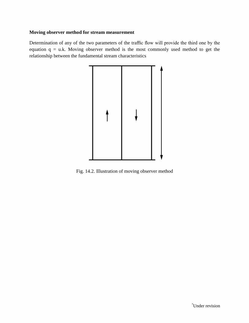
Moving observer method for stream measurement

Determination of any of the two parameters of the traffic flow will provide the third one by the

equation q = u.k. Moving observer method is the most commonly used method to get the

relationship between the fundamental stream characteristics

Fig. 14.2. Illustration of moving observer method

*Under revision

Lecture 15

Capacity and Level of Service

Overview

Capacity and Level of service are two related terms. Capacity analysis tries to give a clear

understanding of how much traffic a given transportation facility can accommodate. Level of

service tries to answer how good the present traffic situation on a given facility is.

Capacity

Capacity is defined as the maximum number of vehicles, passengers, or the like, per unit time,

which can be accommodated under given conditions with a reasonable expectation of

occurrence. Some of the observations that are found from this definition can be now discussed.

Level of service

A term closely related to capacity and often confused with it is service volume. When capacity

gives a quantitative measure of traffic, level of service or LOS tries to give a qualitative measure.

Highway capacity

Highway capacity is defined by the Highway Capacity Manual as the maximum hourly rate at

which persons or vehicles can be reasonably expected to traverse a point or a uniform segment of

a lane or roadway during a given time period under prevailing roadway, traffic and control

conditions.

Traffic conditions:

Road way characteristics:

Control conditions:

Factors affecting level of service

Level of service one can derive from a road under different operating characteristics and

traffic volumes. The factors affecting level of service (LOS) can be listed as follows:

Speed and travel time

Traffic interruptions/restrictions

Freedom to travel with desired speed

Driver comfort and convenience

Operating cost.

*Under revision

Lecture 16

Traffic Sign

Overview

Traffic control device is the medium used for communicating between traffic engineer and road

users. Unlike other modes of transportation, there is no control on the drivers using the road.

Here traffic control devices comes to the help of the traffic engineer. The major types of traffic

control devices used are-

1. Traffic signs

2. Road markings

3. Traffic signals

4. Parking control.

Requirements of traffic control devices

The control device should fulfill a need

It should command attention from the road users

It should convey a clear, simple meaning

Road users must respect the signs

The control device should provide adequate time for proper response from the road users

Types of traffic signs

1. Regulatory signs

2. Warning signs

3. Informative signs

Regulatory signs

These signs are also called mandatory signs because it is mandatory that the drivers must obey

these signs. If the driver fails to obey them, the control agency has the right to take legal action

against the driver.

Right of way series

Speed series

Movement series

Parking series

Pedestrian series

Miscellaneous

*Under revision

Warning signs

Warning signs or cautionary signs give information to the driver about the impending road

condition. They advice the driver to obey the rules.

Informative signs

Informative signs also called guide signs, are provided to assist the drivers to reach their desired

destinations. These are predominantly meant for the drivers who are unfamiliar to the place. The

guide signs are redundant for the users who are accustomed to the location.

Fig.16.1 Examples of informative signs

*Under revision

Lecture 17

Road Sign

Overview

The essential purpose of road markings is to guide and control traffic on a highway. They

supplement the function of traffic signs. The markings serve as a psychological barrier and

signify the delineation of traffic path and its lateral clearance from traffic hazards for the safe

movement of traffic. Hence they are very important to ensure the safe, smooth and harmonious

flow of traffic.

Classification of road markings

The road markings are defined as lines, patterns, words or other devices, except signs, set into

applied or attached to the carriageway or kerbs or to objects within or adjacent to the

carriageway, for controlling, warning, guiding and informing the users. The road markings are

classified as

Longitudinal markings

Transverse markings

Object markings

Word messages

Marking for parking

Marking at hazardous locations

Longitudinal markings

Longitudinal markings are placed along the direction of traffic on the roadway surface, for the

purpose of indicating to the driver, his proper position on the roadway.

Fig.17.1 Centre line marking for a two lane road

*Under revision

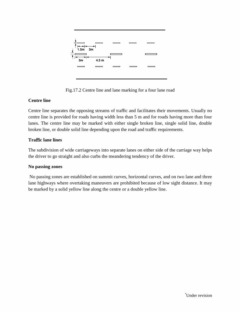
Fig.17.2 Centre line and lane marking for a four lane road

Centre line

Centre line separates the opposing streams of traffic and facilitates their movements. Usually no

centre line is provided for roads having width less than 5 m and for roads having more than four

lanes. The centre line may be marked with either single broken line, single solid line, double

broken line, or double solid line depending upon the road and traffic requirements.

Traffic lane lines

The subdivision of wide carriageways into separate lanes on either side of the carriage way helps

the driver to go straight and also curbs the meandering tendency of the driver.

No passing zones

No passing zones are established on summit curves, horizontal curves, and on two lane and three

lane highways where overtaking maneuvers are prohibited because of low sight distance. It may

be marked by a solid yellow line along the centre or a double yellow line.

*Under revision

Lecture 18

Parking

Overview

Parking is one of the major problems that is created by the increasing road traffic.

Parking studies

Before taking any measures for the betterment of conditions, data regarding availability of

parking space, extent of its usage and parking demand is essential. It is also required to estimate

the parking fares also.

Parking statistics

Parking accumulation

Parking volume

Parking load

Average parking duration

Parking turnover

Parking index

Parking surveys

o In-out survey

o Fixed period sampling

o License plate method of survey

On street parking

Parallel parking

30 parking

45 parking

60 parking

Right angle parking

Off street

Parking In many urban centres, some areas are exclusively allotted for parking which will be at

some distance away from the main stream of traffic. Such a parking is referred to as off-street

parking.

*Under revision

Lecture 19

Traffic Signal Design

Overview

The conflicts arising from movements of traffic in different directions is solved by time sharing

of the principle. The advantages of traffic signal includes an orderly movement of traffic, an

increased capacity of the intersection and requires only simple geometric design. However the

disadvantages of the signalized intersection are it affects larger stopped delays, and the design

requires complex considerations.

Definitions and notations

Cycle

Cycle length

Interval

Green interval

Red interval

Phase

Lost time

Phase design

The signal design procedure involves six major steps.

They include the

1. phase design

2. determination of amber time and clearance time

3. determination of cycle length

4. apportioning of green time

5. pedestrian crossing requirements,

6. the performance evaluation

Two phase signals

Two phase system is usually adopted if through traffic is significant compared to the turning

movements.

*Under revision

Fig. 19.1 Two phase signal

Four phase signals

There are at least three possible phasing options.

Fig.19.2 One way of providing four phase signals

Cycle time

Cycle time is the time taken by a signal to complete one full cycle of iterations. i.e. one

complete rotation through all signal indications. It is denoted by C.

Fig.19.3 Headways departing signal

*Under revision

Lecture 20

Subgrade Material

Overview

Pavements are a conglomeration of materials. These materials, their associated properties, and

their interactions determine the properties of the resultant pavement.

Sub grade soil

Soil is an accumulation or deposit of earth material, derived naturally from the disintegration of

rocks or decay of vegetation, that can be excavated readily with power equipment in the field or

disintegrated by gentle mechanical means in the laboratory.

Desirable properties

The desirable properties of sub grade soil as a highway material are

1. Stability

2. Incompressibility

3. Permanency of strength

4. Minimum changes in volume and stability

5. Good drainage

6. Ease of compaction

Soil Classification

Two commonly used systems for soil engineers based on particle distribution and atterberg

limits:

•American Association of State Highway and Transportation Officials (AASHTO) System (for

state/county highway dept.)

•Unified Soil Classification System (USCS) (preferred by geotechnical engineers).

Soil particles

The description of the grain size distribution of soil particles according to their texture (particle

size, shape, and gradation).Major textural classes include, very roughly:

gravel (>2 mm);

sand (0.1 –2 mm);

silt (0.01 –0.1 mm);

clay (< 0.01 mm).

*Under revision

Lecture 21

Test of Soil

Overview

Sub grade soil is an integral part of the road pavement structure as it provides the support to the

pavement from beneath. The main function of the sub grade is to give adequate support to the

pavement and for this the sub grade should possess sufficient stability under adverse climatic and

loading conditions. Therefore, it is very essential to evaluate the sub grade by conducting tests.

The tests used to evaluate the strength properties of soils may be broadly divided into three

groups:

1. Shear tests

2. Bearing tests

3. Penetration tests

Shear tests

Shear tests are usually carried out on relatively small soil samples in the laboratory. In order to

find out the strength properties of soil, a number of representative samples from different

locations are tested. Some of the commonly known shear tests:

o Direct shear test,

o Triaxial compression test,

o Unconfined compression test.

California Bearing Ratio (CBR)

This test was developed by the California Division of Highway as a method of classifying and

evaluating soil-sub grade and base course materials for flexible pavements.

Fig 21.1 CBR Test

*Under revision

Plate Bearing Test

Plate bearing test is used to evaluate the support capability of sub-grades, bases and in some

cases, complete pavement. Data from the tests are applicable for the design of both flexible and

rigid pavements. In plate bearing test, a compressive stress is applied to the soil or pavement

layer through rigid plates relatively large size and the deflections are measured for various stress

values.

Fig.21.2 Plate load test

*Under revision

Lecture 22

Pavement materials

Overview

Aggregate is a collective term for the mineral materials such as sand, gravel, and crushed stone

that are used with a binding medium (such as water, bitumen, Portland cement, lime, etc.) to

form compound materials (such as bituminous concrete and Portland cement concrete). By

volume, aggregate generally accounts for 92 to 96 percent of Bituminous concrete and about 70

to 80 percent of Portland cement concrete. Aggregate is also used for base and sub-base courses

for both flexible and rigid pavements. Aggregates can either be natural or manufactured.

Desirable properties

Strength

The aggregates used in top layers are subjected to

(i) Stress action due to traffic wheel load,

(ii) Wear and tear,

(iii) crushing.

Hardness

The aggregates used in the surface course are subjected to constant rubbing or abrasion due to

moving traffic. The aggregates should be hard enough to resist the abrasive action caused by the

movements of traffic. The abrasive action is severe when steel tyred vehicles moves over the

aggregates exposed at the top surface.

Toughness

Resistance of the aggregates to impact is termed as toughness. Aggregates used in the pavement

should be able to resist the effect caused by the jumping of the steel tyred wheels from one

particle to another at different levels causes severe impact on the aggregates.

Shape of aggregates

Aggregates which happen to fall in a particular size range may have rounded cubical, angular,

flaky or elongated particles. It is evident that the aky and elongated particles will have less

strength and durability when compared with cubical, angular or rounded particles of the same

aggregate. Hence too flaky and too much elongated aggregates should be avoided as far as

possible.

*Under revision

Adhesion with bitumen

The aggregates used in bituminous pavements should have less a nity with water when compared

with bituminous materials, otherwise the bituminous coating on the aggregate will be stripped o

in presence of water.

Durability

The property of aggregates to withstand adverse action of weather is called soundness. The

aggregates are subjected to the physical and chemical action of rain and bottom water, impurities

there-in and that of atmosphere, hence it is desirable that the road aggregates used in the

construction should be sound enough to withstand the weathering action

Freedom from deleterious particles

Specifications for aggregates used in bituminous mixes usually require the aggregates to be

clean, tough and durable in nature and free from excess amount of at or elongated pieces, dust,

clay balls and other objectionable material. Similarly aggregates used in Portland cement

concrete mixes must be clean and free from deleterious substances such as clay lumps, chert, silt

and other organic impurities.

*Under revision

Lecture 23

Aggregate tests-I

Overview

In order to decide the suitability of the aggregate for use in pavement construction, following

tests are carried out:

Crushing test

Abrasion test

Impact test

Soundness test

Shape test

Specific gravity and water absorption test

Bitumen adhesion test

Crushing test One of the model in which pavement material can fail is by crushing under compressive stress. A test is

standardized by IS:2386 part-IV and used to determine the crushing strength of aggregates. The

aggregate crushing value provides a relative measure of resistance to crushing under gradually applied

crushing load.

Fig.23.1 Crushing test setup

Abrasion test Abrasion test is carried out to test the hardness property of aggregates and to decide whether they are suitable for

different pavement construction works. Los Angeles abrasion test is a preferred one for carrying out the hardness

property and has been standardized in India (IS:2386 part-IV).

*Under revision

Fig.23.2 Los Angeles abrasion test setup

Impact test

The aggregate impact test is carried out to evaluate the resistance to impact of aggregates.

Aggregates passing 12.5 mm sieve and retained on 10 mm sieve is filled in a cylindrical steel

cup of internal dia 10.2 mm and depth 5 cm which is attached to a metal base of impact testing

machine. The material is filled in 3 layers where each layer is tamped for 25 number of blows.

Soundness test

Soundness test is intended to study the resistance of aggregates to weathering action, by

conducting accelerated weathering test cycles. The Porous aggregates subjected to freezing and

thawing are likely to disintegrate prematurely. To ascertain the durability of such aggregates,

they are subjected to an accelerated soundness test as specified in IS:2386 part-V.

Fig.23.3 Impact test setup

*Under revision

Lecture 24

Aggregate tests-II

Shape tests

The particle shape of the aggregate mass is determined by the percentage of flaky and elongated

particles in it. Aggregates which are flaky or elongated are detrimental to higher workability and

stability of mixes. The flakiness index is defined as the percentage by weight of aggregate

particles whose least dimension is less than 0.6 times their mean size. Test procedure had been

standardized in India (IS:2386 part-I).

Fig.24.1 Flakiness gauge

Fig.24.2 Elongation gaugege

Specific Gravity and water absorption The Specific gravity and water absorption of aggregates are important properties that are

required for the design of concrete and bituminous mixes. The Specific gravity of a solid is the

ratio of its mass to that of an equal volume of distilled water at a specified temperature.

Apparent Specific Gravity

Bulk Specific Gravity

Water absorption, The difference between the apparent and bulk specific gravities is nothing but

the water- permeable voids of the aggregates.

*Under revision

The specific gravity of aggregates normally used in road construction ranges from about 2.5 to 2.9. Water

absorption values ranges from 0.1 to about 2.0 percent for aggregates normally used in road surfacing.

Bitumen adhesion test

Bitumen adheres well to all normal types of road aggregates provided they are dry and free from dust. In

the absence of water there is practically no adhesion problem of bituminous construction. Adhesion

problem occurs when the aggregate is wet and cold.

Table 24.1 Tests for Aggregates with IS codes

*Under revision

Lecture 25

Pavement materials: Bitumen

Overview

Bituminous materials or asphalts are extensively used for roadway construction, primarily

because of their excellent binding characteristics and water proofing properties and relatively

low cost.

Production of Bitumen

Bitumen is the residue or by-product when the crude petroleum is refined. A wide variety of

refinery processes, such as the straight distillation process, solvent extraction process etc. may be

used to produce bitumen of different consistency and other desirable properties.

Vacuum steam distillation of petroleum oils

In the vacuum-steam distillation process the crude oil is heated and is introduced into a large

cylindrical still. Steam is introduced into the still to aid in the vaporization of the more volatile

constituents of the petroleum and to minimize decomposition of the distillates and residues. The

volatile constituents are collected, condensed, and the various fractions stored for further

refining, if needed. The residues from this distillation are then fed into a vacuum distillation unit,

where residue pressure and steam will further separate out heavier gas oils. The bottom fraction

from this unit is the vacuum-steam-re ned asphalt cement.

Different forms of bitumen

Cutback bitumen

Normal practice is to heat bitumen to reduce its viscosity. In some situations preference is given

to use liquid binders such as cutback bitumen. In cutback bitumen suitable solvent is used to

lower the viscosity of the bitumen. From the environmental point of view also cutback bitumen

is preferred.

There are different types of cutback bitumen like rapid curing (RC), medium curing (MC), and

slow curing (SC).

Bitumen emulsion

Bitumen emulsion is a liquid product in which bitumen is suspended in a finely divided

condition in an aqueous medium and stabilized by suitable material. Three types of bituminous

emulsions are available, which are Rapid setting (RS), Medium setting (MS), and Slow setting

(SC). Bitumen emulsions are ideal binders for hill road construction.

*Under revision

Bituminous primers

In bituminous primer the distillate is absorbed by the road surface on which it is spread. The

absorption therefore depends on the porosity of the surface. Bitumen primers are useful on the

stabilized surfaces and water bound macadam base courses. Bituminous primers are generally

prepared on road sites by mixing penetration bitumen with petroleum distillate.

Modified Bitumen

Certain additives or blend of additives called as bitumen modifiers can improve properties of

Bitumen and bituminous mixes. Bitumen treated with these modifiers is known as modified

bitumen. Polymer modified bitumen (PMB)/ crumb rubber modified bitumen (CRMB) should be

used only in wearing course depending upon the requirements of extreme climatic variations.

The detailed specifications for modified bitumen have been issued by IRC: SP: 53-1999.

Requirements of Bitumen

The desirable properties of bitumen depend on the mix type and construction. In general,

Bitumen should posses following desirable properties.

o The bitumen should not be highly temperature susceptible: during the hottest weather the

mix should not become too soft or unstable, and during cold weather the mix should not

become too brittle causing cracks.

o The viscosity of the bitumen at the time of mixing and compaction should be adequate.

This can be achieved by use of cutbacks or emulsions of suitable grades or by heating the

bitumen and aggregates prior to mixing.

o There should be adequate affinity and adhesion between the bitumen and aggregates used

in the mix.

*Under revision

Lecture 26

Test of Bitumen

Tests on bitumen

There are a number of tests to assess the properties of bituminous materials. The following tests

are usually conducted to evaluate di erent properties of bituminous materials.

Penetration test

Ductility test

Softening point test

Specific gravity test

Viscosity test

Flash and Fire point test

Float test

Water content test

Loss on heating test

Penetration test It measures the hardness or softness of bitumen by measuring the depth in tenths of a millimeter

to which a standard loaded needle will penetrate vertically in 5 seconds. BIS had standardized

the equipment and test procedure. The penetrometer consists of a needle assembly with a total

weight of 100g and a device for releasing and locking in any position.

Fig. 26. 1 Penetration Test Setup

Ductility test

Ductility is the property of bitumen that permits it to undergo great deformation or elongation.

Ductility is defined as the distance in cm, to which a standard sample or briquette of the material

will be elongated without breaking.

*Under revision

Fig. 26.2 Ductility Moulds

Softening point test

Softening point denotes the temperature at which the bitumen attains a particular degree of

softening under the specifications of test. The test is conducted by using Ring and Ball apparatus.

Fig. 26.3 Softening Point Test Setup

Specific gravity test

In paving jobs, to classify a binder, density property is of great use. In most cases bitumen is

weighed, but when used with aggregates, the bitumen is converted to volume using density

values. The density of bitumen is greatly influenced by its chemical composition. Increase in

aromatic type mineral impurities cause an increase in specific gravity.

Viscosity test

Viscosity denotes the fluid property of bituminous material and it is a measure of resistance to

flow. At the application temperature, this characteristic greatly influences the strength of

resulting paving mixes. Low or high viscosity during compaction or mixing has been observed to

*Under revision

result in lower stability values. At high viscosity, it resist the compactive effort and thereby

resulting mix is heterogeneous, hence low stability values.

Fig.26.4 Viscosity apparatus

Flash and fire point test

At high temperatures depending upon the grades of bitumen materials leave out volatiles. And

these volatiles catches fire which is very hazardous and therefore it is essential to qualify this

temperature for each bitumen grade.

Float test

Normally the consistency of bituminous material can be measured either by penetration test or

viscosity test. But for certain range of consistencies, these tests are not applicable and Float test

is used.

Water content test

It is desirable that the bitumen contains minimum water content to prevent foaming of the

bitumen when it is heated above the boiling point of water. The water in a bitumen is determined

by mixing known weight of specimen in a pure petroleum distillate free from water, heating and

distilling of the water.

Loss on heating test

When the bitumen is heated it loses the volatility and gets hardened. About 50gm of the sample

is weighed and 0 heated to a temperature of 163 C for 5hours in a specified oven designed for

this test.

*Under revision

Lecture 27

Bituminous Mix Design-I

Overview

The bituminous mix design aims to determine the proportion of bitumen, filler, fine aggregates,

and coarse aggregates to produce a mix which is workable, strong, durable and economical. The

requirements of the mix design and the two major stages of the mix design, i.e dry mix design

and wet mix design.

Objectives of mix design

1. Sufficient bitumen to ensure a durable pavement,

2. Sufficient strength to resist shear deformation under traffic at higher temperature,

3. Sufficient air voids in the compacted bitumen to allow for additional compaction by traffic,

4. Sufficient workability to permit easy placement without segregation,

5. Sufficient flexibility to avoid premature cracking due to repeated bending by traffic,and

6. Sufficient flexibility at low temperature to prevent shrinkage cracks.

Constituents of a mix

Coarse aggregates

Fine aggregates

Filler

Binder

Types of mix

Well-graded mix

Gap-graded mix

Open-graded mix

Unbounded

Different layers in a pavement

o Bituminous base course

o Bituminous binder course

o Asphaltic/Bituminous concrete

*Under revision

Lecture 28

Requirements of Bituminous mixes

Stability

Stability is defined as the resistance of the paving mix to deformation under traffic load. Two

examples of failure are

(i) shoving - a transverse rigid deformation which occurs at areas subject to severe acceleration

(ii) grooving - longitudinal ridging due to channelization of traffic. Stability depend on the inter-

particle friction, primarily of the aggregates and the cohesion offered by the bitumen.

Durability

Durability is defined as the resistance of the mix against weathering and abrasive actions.

(i) pot-holes, - deterioration of pavements locally and

(ii) stripping, lost of binder from the aggregates and aggregates are exposed.

Flexibility

Flexibility is a measure of the level of bending strength needed to counteract traffic load and

prevent cracking of surface. Fracture is the cracks formed on the surface (hairline-cracks,

alligator cracks), main reasons are shrinkage and brittleness of the binder.

Skid resistance

It is the resistance of the finished pavement against skidding which depends on the surface

texture and bitumen content. It is an important factor in high speed traffic.

Workability

Workability is the ease with which the mix can be laid and compacted, and formed to the

required condition and shape.

Desirable properties

From the above discussion, the desirable properties of a bituminous mix can be summarized as

follows:

Stability to meet traffic demand

Bitumen content to ensure proper binding and water proofing

Voids to accommodate compaction due to traffic

Flexibility to meet traffic loads, esp. in cold season

Sufficient workability for construction • Economical mix

*Under revision

Lecture 29

Dry Mix Design

Overview

The objective of dry mix design is to determine the amount of various sizes of mineral

aggregates to use to get a mix of maximum density. The dry mix design involves three important

steps, viz. selection of aggregates, aggregates gradation, and proportion of aggregates, which are

discussed below.

Selection of aggregates

The desirable qualities of a bituminous paving mixture are dependent to a considerable degree on

the nature of the aggregates used. Aggregates are classified as coarse, fine, and filler. The

function of the coarse aggregates in contributing to the stability of a bituminous paving mixture

is largely due to interlocking and frictional resistance of adjacent particles.

Aggregate gradation

The properties of the bituminous mix including the density and stability are very much

dependent on the aggregates and their grain size distribution.

However, some minimum amount of void space is necessary to:

o provide adequate volume for the binder to occupy,

o promote rapid drainage, and

o provide resistance to frost action for base and sub base courses.

Proportioning of aggregates

After selecting the aggregates and their gradation, proportioning of aggregates has to be done

and following are the common methods of proportioning of aggregates:

• Trial and error procedure:

• Graphical Methods:

• Analytical Method:

*Under revision

Lecture 30

Marshall Mix Design

Overview

The mix design (wetmix) determines the optimum bitumen content. This is preceded by the dry

mix design.

Marshall mix design

The Marshall stability and flow test provides the performance prediction measure for the

Marshall mix design method. The stability portion of the test measures the maximum load

supported by the test specimen at a loading rate of 50.8 mm/minute.

Specimen preparation

Determine the properties of the mix

Fig. 30.1 Marshall Mould

Fig. 30.2 Marshall Mould

*Under revision

Theoretical specific gravity of the mix Gt

Bulk specific gravity of mix Gm

Air voids percent Vv

Voids in mineral aggregateVMA

Voids filled with bitumen VFB

Determine Marshall stability and flow

Marshall stability of a test specimen is the maximum load required to produce failure when the

specimen is preheated to a prescribed temperature placed in a special test head and the load is

applied at a constant strain (5 cm per minute).

Apply stability correction

*Under revision

Prepare graphical plots

The average value of the above properties are determined for each mix with different bitumen

content and the following graphical plots are prepared:

1. Binder content versus corrected Marshall stability

2. Binder content versus Marshall flow

3. Binder content versus percentage of void in the total mix v

4. Binder content versus voids filled with bitumen (V F B) 5. Binder content versus unit weight

or bulk specific gravity

Determine optimum bitumen content

Determine the optimum binder content for the mix design by taking average value of the

following three bitumen contents found form the graphs obtained in the previous step.

1. Binder content corresponding to maximum stability

2. Binder content corresponding to maximum bulk specific gravity

3. Binder content corresponding to the median of designed limits of percent air voids in the total

mix v (i.e. 4%)

Fig. 30.1 Marshal graphical plots

*Under revision

Lecture 31

Flexible pavement design-I

Overview

Flexible pavements are so named because the total pavement structure deflects, or flexes, under

loading. A flexible pavement structure is typically composed of several layers of materials. Each

layer receives loads from the above layer, spreads them out, and passes on these loads to the next

layer below. Thus the stresses will be reduced, which are maximum at the top layer and

minimum on the top of subgrade.

Design procedures

Empirical design

Empirical design

Traffic and Loading

Fixed traffic

Fixed vehicle

Variable traffic and vehicle

Equivalent single wheel load

To carry maximum load with in the specified limit and to carry greater load, dual wheel, or dual

tandem assembly is often used. Equivalent single wheel load (ESWL) is the single wheel load

having the same contact pressure, which produces same value of maximum stress, deflection,

tensile stress or contact pressure at the desired depth.

Equivalent single wheel load To carry maximum load with in the specified limit and to carry

greater load, dual wheel, or dual tandem assembly is often used. Equivalent single wheel load

(ESWL) is the single wheel load having the same contact pressure, which produces same value

of maximum stress, deflection, tensile stress or contact pressure at the desired depth.

*Under revision

Fig. 31.1 ESWL-Equal stress concept

Equivalent single axle load

o Legal axle load

o Standard axle load

Repetition of axle loads

Equivalent axle load factor

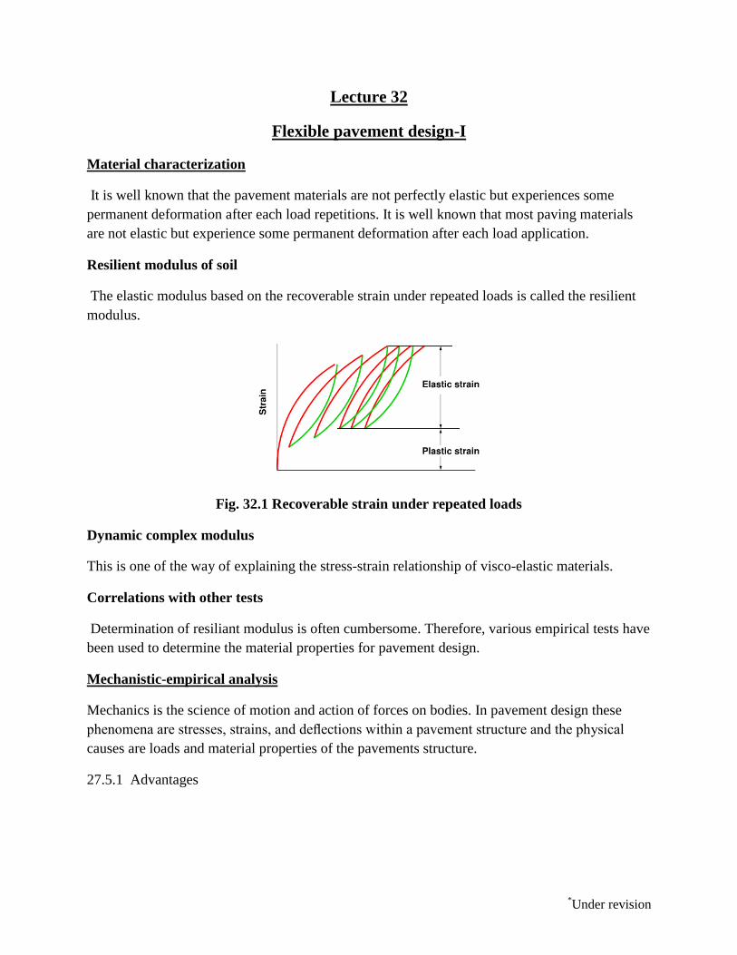
*Under revision

Lecture 32

Flexible pavement design-I

Material characterization

It is well known that the pavement materials are not perfectly elastic but experiences some

permanent deformation after each load repetitions. It is well known that most paving materials

are not elastic but experience some permanent deformation after each load application.

Resilient modulus of soil

The elastic modulus based on the recoverable strain under repeated loads is called the resilient

modulus.

Fig. 32.1 Recoverable strain under repeated loads

Dynamic complex modulus

This is one of the way of explaining the stress-strain relationship of visco-elastic materials.

Correlations with other tests

Determination of resiliant modulus is often cumbersome. Therefore, various empirical tests have

been used to determine the material properties for pavement design.

Mechanistic-empirical analysis

Mechanics is the science of motion and action of forces on bodies. In pavement design these

phenomena are stresses, strains, and deflections within a pavement structure and the physical

causes are loads and material properties of the pavements structure.

27.5.1 Advantages

*Under revision

The basic advantages of the Mechanistic-Empirical pavement design method over a purely

empirical one are:

o It can be used for both existing pavement rehabilitation and new pavement construction

o It can accommodate changing load types

o It can better characterize materials allowing for better utilization of available materials

accommodation of new materials improved definition of existing layer proportion

o It uses material proportion that relates better with actual pavement performance

o It provides more reliable performance predictions

o It defines role of construction in a better way

o It accommodates environment and aging e ect of materials in the pavement

Mechanistic model

Mechanistic models are used to mathematically model pavement physics.

Inputs A layered elastic model requires a minimum number of inputs to adequately characterize a

pavement structure and its response to loading. These inputs are:

Material properties of each layer, like modulus of elasticity (E), Poisson's ratio,

Pavement layer thicknesses, and Loading conditions which include the total wheel load and load repetitions

Output The outputs of the layered elastic model are the stresses, strains and de ections in the pavements. Stress.

Strain.

Deflection.

*Under revision

Lecture 33

IRC Method of Flexible Pavement Design

Overview

Indian roads congress has specified the design procedures for exible pavements based on CBR

values. The Pavement designs given in the previous edition IRC:37-1984 were applicable to

design traffic upto only 30 million standard axles (msa).

Scope

These guidelines will apply to design of exible pavements for Expressway, National Highways,

State Highways, Major District Roads, and other categories of roads. Flexible pavements are

considered to include the pavements which have bituminous surfacing and granular base and

sub-base courses conforming to IRC/ MOST standards. These guidelines apply to new

pavements.

Design criteria

o Vertical compressive strain at the top of the sub-grade which can cause sub-grade

deformation resulting in permanent deformation at the pavement surface.

o Horizontal tensile strain or stress at the bottom of the bituminous layer which can cause

fracture of the bituminous layer.

o Pavement deformation within the bituminous layer.

Failure Criteria

Fatigue Criteria

Rutting Criteria

Fig. 33.1 Critical Locations in Pavement

*Under revision

Design procedure

Based on the performance of existing designs and using analytical approach, simple design

charts and a catalogue of pavement designs are added in the code.

Using the following simple input parameters, appropriate designs could be chosen for the given

traffic and soil strength:

Design traffic in terms of cumulative number of standard axles; and

CBR value of subgrade.

Design traffic

The method considers traffic in terms of the cumulative number of standard axles (8160 kg) to be

carried by the pavement during the design life. This requires the following information:

Initial traffic in terms of CVPD

Traffic growth rate during the design life

Design life in number of years

Vehicle damage factor (VDF)

Distribution of commercial traffic over the carriage way.

Pavement thickness design charts

For the design of pavements to carry traffic in the range of 1 to 10 msa, use chart 1 and for traffic

in the range 10 to 150 msa, use chart 2 of IRC:37 2001.

Pavement composition

o Sub-base

o Base

o Bituminous surfacing

*Under revision

Lecture 34

Stresses in Rigid Pavement

Overview

As the name implies, rigid pavements are rigid i.e, they do not flex much under loading like

flexible pavements. They are constructed using cement concrete. In this case, the load carrying

capacity is mainly due to the rigidity ad high modulus of elasticity of the slab (slab action).

Modulus of sub-grade reaction

Westergaard considered the rigid pavement slab as a thin elastic plate resting on soil sub-grade,

which is assumed as a dense liquid. The upward reaction is assumed to be proportional to the

deflection.

Relative stiffness of slab to sub-grade

A certain degree of resistance to slab deflection is offered by the sub-grade. The sub-grade

deformation is same as the slab deflection. Hence the slab deflection is direct measurement of the

magnitude of the sub-grade pressure.

Critical load positions

There are three typical locations namely the interior, edge and corner, where differing conditions

of slab continuity exist. These locations are termed as critical load positions.

Fig. 34.1 Critical stress locations

Temperature stresses

Temperature stresses are developed in cement concrete pavement due to variation in slab

temperature. This is caused by

(i) Daily variation resulting in a temperature gradient across the thickness of the slab and

*Under revision

(ii) Seasonal variation resulting in overall change in the slab temperature.

Combination of stresses

The cumulative effect of the different stress give rise to the following thee critical cases

Summer, mid-day: The critical stress is for edge region

Winter, mid-day: The critical combination of stress is for the edge region given by

Mid-nights: The critical combination of stress is for the corner region given

*Under revision

Lecture 35

Design of joints

Expansion joints

The purpose of the expansion joint is to allow the expansion of the pavement due to rise in

temperature with respect to construction temperature.

Fig. 35.1 Expansion joint

Contraction joints

35.2 Contraction Joint

Dowel bars

The purpose of the dowel bar is to effectively transfer the load between two concrete slabs and to keep the

two slabs in same height.

Tie bars

In contrast to dowel bars, tie bars are not load transfer devices, but serve as a means to tie two

slabs. Hence tie bars must be deformed or hooked and must be firmly anchored into the concrete

to function properly.

*Under revision

Lecture 36

Low Volume Roads

Overview

Low Volume Road is considered a road that has relatively low use (an Average Daily Traffic of

less than 400 vehicles per day), low design speeds (typically less than 80 kph), and

corresponding geometry. Most roads in rural areas are low-volume roads.

Steps

The basic steps of road panning are:

o Planning

o Location

o Survey

o Design

o Construction

o Maintenance

Importance of Rural Roads

Rural road connectivity is a key component of rural development in India since it promotes

access to economic and social services and thereby increases agricultural income and productive

employment opportunities. As a result, it is also a key ingredient in ensuring sustainable poverty

reduction.

Aspect of Road Design

o General Design

o Materials

o Slopes

o Drainage

o Erosion Control

*Under revision

Lecture 37

Highway Drainage

Overview

Provision for adequate drainage is of paramount importance in road design and cannot be

overemphasized. The presence of excess water or moisture within the roadway will adversely

affect the engineering properties of the materials with which it was constructed. Cut or fill

failures, road surface erosion, and weakened subgrades followed by a mass failure are all

products of inadequate or poorly designed drainage. As has been stated previously, many

drainage problems can be avoided in the location and design of the road: Drainage design is most

appropriately included in alignment and gradient planning.

Importance of Drainage

Water has a number of unhelpful characteristics which impact on highway performance.

o It is a lubricant reducing the effectiveness of tyre grip on the carriageway wearing surface

which can increase stopping distances.

o Spray from rainwater being thrown up by car tyres can reduce visibility which can lead to

delays in reacting to events on the carriageway.

o Drag on car tyres from local rainwater ponding can alter the balance of vehicles travelling

at speed which can be alarming or cause skidding.

o It is incompressible therefore standing water effectively acts as a jackhammer on the

wearing course right through to the sub-base when vehicles pass over head.

o It expands when frozen pulling apart the carriageway construction which then falls apart

when it warms up

o In extreme storms, rainwater can simply wash away roads on embankment should the

culvert become blocked or lack capacity.

*Under revision

Lecture 38

Bridge Engineering-I

Classification of Bridges

1.Classification of Bridges (According to form (or) type of superstructures) •Slab bridge

•Beam bridge

•Truss bridge

•Arch bridge

•Cable stayed (or )suspended bridge

2.Classification of bridges (According to material of construction of superstructure) •Timber bridge

•Concrete bridge

•Stone bridge

•R.C.C bridge

•Steel bridge

•P.C.C bridge

•Composite bridge

•Aluminum bridge

3. Classification of bridges (According to inter-span relationship) •Simply supported bridge

•Cantilever bridge

•Continuous bridge

4. Classification of bridges (According to the position of the bridge floor relative to

superstructures) •Deck through bridge

•Half through or suspension bridge

5. Classification of bridges (According to method of connection of different part of

superstructures) •Pinned connection bridge

•Riveted connection bridge

•Welded connection bridge

6.Classification of bridges (According to length of bridge) •Culvert bridge(less than 6 m)

•Minor bridge(less than 6 m-60m)

•Major bridge(more than 60 m)

•Long span bridge(more than 120 m)

*Under revision

9.Classification of bridges (According to function) •Aqueduct bridge(canal over a river)

•Viaduct(road or railway over a valley or river)

•Pedestrian bridge

•Highway bridge

•Railway bridge

•Road-cum-rail or pipe line bridge

Bridge scour

It is the removal of sediment such as sand and rocks from around bridge abutments or piers.

Scour, caused by swiftly moving water, can scoop out scour holes, compromising the integrity of

a structure.

In the United States of America, bridge scour is one of the three main causes of bridge failure

(the others being collision and overloading). It has been estimated that 60% of all bridge failures

result from scour and other hydraulic-related causes. It is the most common cause of highway

bridge failure in the United States, where 46 of 86 major bridge failures resulted from scour near

piers from 1961 to 1976.

*Under revision

Lecture 39

Bridge Engineering-II

Shallow Foundations:

Foundations provided immediately beneath the lowest part of the structure, near to the ground

level are known as shallow foundations. Such foundations are mostly placed on the first hard and

firm strata available below the ground level. Shallow foundations are further classified into the

following types:

1. Spread footing or open trench foundations

2. Grillage foundations

3. Raft foundations

4. Stepped foundations

5. Inverted arch foundations

Deep Foundation:

The foundation constructed sufficiently below ground level with some artificial arrangements

such as piles, wells etc, at their base are called deep foundations. Deep foundation are further

classified into the following types;

1. Pile foundation

2. Well foundation

3. Caisson foundation

*Under revision

Lecture 40

Earthwork

For various civil engineering projects like road work, irrigation canal project, tank survey, earth

moving, etc, the calculation method used are different. Some of these methods were introduced

before the invention of computers and are still being continued. This document discusses about

the industry practices of various methods of volume calculation so that the users can finally

choose the right one for their project.

Earthworks Earthworks are engineering works created through the moving and/or processing of massive

quantities of soil or unformed rock. Earthwork is done to reconfigure the topography of a site to

achieve the design levels. Earthwork involves cutting and filling to achieve the required

topography.

Cutting

Cutting is the process of excavating earth material from a work location to achieve the desired

topography.

Filling Filling is the process of moving the excavated material or additional earth material to a work

location to achieve the desired topography.

Applications of Earthwork Typically, earthwork is done in the following projects:

Road works

Railways

Irrigation project such as canals and dams

Other common earthwork applications are land grading to reconfigure the topography of

a site, or to stabilize slopes

Trapezoidal Rule (End Area)

In trapezoidal method, each segment of the section is divided into various trapezoids and

triangles.

Trapezoidal Area A = 1/2 X a X (b1+b2)

*Under revision

Triangle area A = a * b/2

*Under revision

Bibliography

1. Khanna, S. K., & Justo, C. E. G. (1991). Highway engineering. Nem Chand & Bros.

2. Mathew, T.V., & Rao, K.V.K. (2007). Introduction to transportation engineering–NPTEL.