
Lecture note 7 discrete event control1 Discrete Event Control CONTENTS 1. Introduction 2. State...
22
Lecture note 7 discrete event control 1 Discrete Event Control CONTENTS 1. Introduction 2. State Diagram 3. Boolean Logical Equation
-
Upload
adam-needler -
Category
Documents
-
view
224 -
download
2
Transcript of Lecture note 7 discrete event control1 Discrete Event Control CONTENTS 1. Introduction 2. State...

Lecture note 7 discrete event control 1
Discrete Event Control
CONTENTS
1. Introduction
2. State Diagram
3. Boolean Logical Equation

Lecture note 7 discrete event control 2
Discrete Event Control
Concept
Representation
DEC controller design
DEC controller implementation

Lecture note 7 discrete event control 3
Discrete Event Control: introduction
DEC: All control variables are discrete variables, and their change is
as a result of the occurrence of events.
Multiple-input/multiple-output (MIMO) discrete logical controller, see
Figure 1, where Ii is discrete value-based input variable, and Yi
discrete value-based output.
Ii and Yi only take value 0 (off) or 1 (on).
Input and output devices are usually located at a distance from the
controller.
Figure 1DiscreteEventControl system

Lecture note 7 discrete event control 4
Figure 2
Introduction
Figure 3
Level Limit Switch LLS
Controller Input valve Tank
Level of Water

Lecture note 7 discrete event control 5
We need a method to represent system dynamics, i.e. control system (including both plant and controller).
However, in a discrete event driven system, plant (transient) dynamics is ignored. This means that when the valve is open, the water level seems to rise to a level instantly.
Therefore, the control system for a discrete event driven system reduces to the controller only.
goal controller plant plant output
State and state diagram is the method to represent system dynamics.
Introduction

Lecture note 7 discrete event control 6
State Diagram States: indicators that system changes
State Variables: assign a name to each independent class of states.
EX 1: Switch. The switch is a state variable. It has two states (1, 0),
where 1=on and 0=off.
State change has a cause.
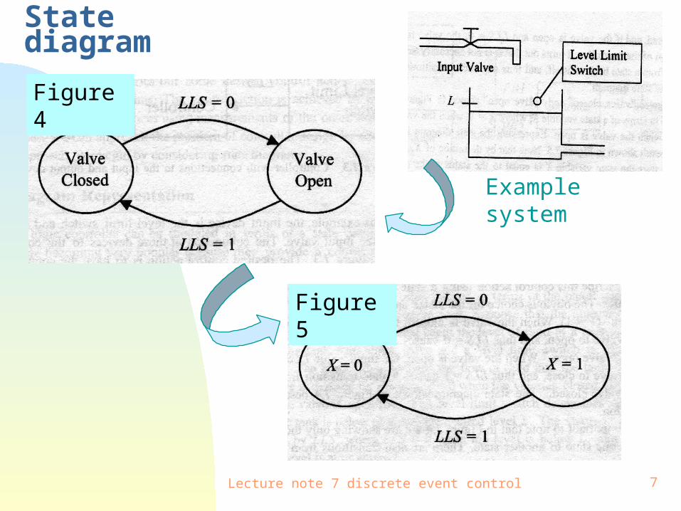
State diagram (Fig. 4, Fig. 5) represents the state change with cause;I
n particular, node: state; edge: cause.
In this example, we define:
LLS=0 for the level of liquid is below L
LLS=1 for the level of liquid is above L
Is LLS state variable?
NO
Lecture note 7 discrete event control 7
State diagram
Example system
Figure 4
Figure 5

Lecture note 7 discrete event control 8
State Diagram
System has input, output, and itself.
Fluid is a part of the system or total system.
System itself includes components, e.g., valve, pump.
System itself is represented by a set of state variables.
The total system has fluid and device, and the device manipulates the fluid.
Level of the fluid in the tank is the output of the plant (e.g., tank) or the plant control system (including both the plant and controller) and the input to the controller.
In the time continuous system, the goal or reference variable such as L (in the tank example) is an input to the control system, while the level of the fluid is the output of the control system.
Lecture note 7 discrete event control 9
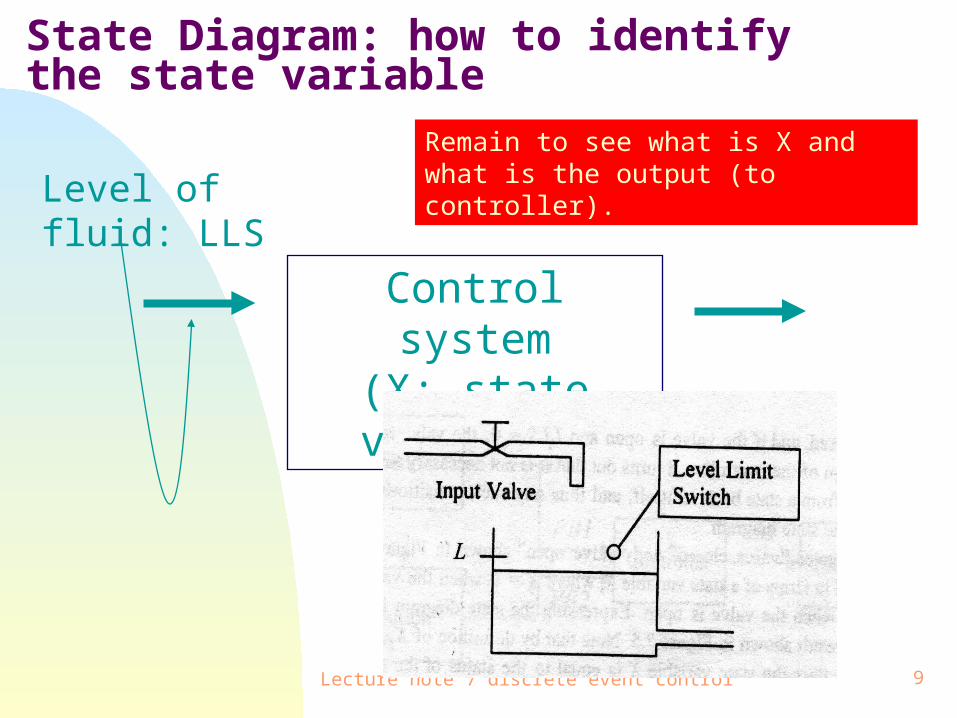
State Diagram: how to identify the state variable
Control system(X: state variable)
Level of fluid: LLS
Remain to see what is X and what is the output (to controller).

Lecture note 7 discrete event control 10
State Diagram
Control system(X: state variable)
Level of fluid: LLS
X: state variable: valve.
Output (for controller): X as well.
So we have: output = state variable of the system

Lecture note 7 discrete event control 11
State Diagram
It is noted that the two circles represent different states of one state
variable (i.e., valve). The system in EX 1 has only one state variable.
EX 2: In EX 1, if we introduce also the pump in the system. In particular,
there is a piece of knowledge: when the valve is closed the pump must be
off. We can sum up the desired control actions as follows:
Pump
Lecture note 7 discrete event control 12
State Diagram
State variables: X1: pump; X2: valve.
X1: X1=0: pump off
X1=1: pump on
X2: X2=0: valve is closed
X2=1: valve is open

Lecture note 7 discrete event control 13
State Diagram (for controller)
1. Open the valve if it is closed and the level of liquid in the tank is less
than the desired level L (LLS=0), or keep the valve open if LLS=0.
2. Close the valve if it is open and the level of liquid in the tank is equal to
or greater than the desired level L (LLS=1), or keep the valve closed if
LLS=1.
3. Turn the pump on if it is off and the valve is open and LLS=0, or keep
the pump on if it is already on and the valve is open and LLS=0.
4. Turn the pump off if it is on and LLS=1, or keep the pump off if
LLS=1.
Lecture note 7 discrete event control 14
State Diagram
The above expressions of control action can be represented by two state variables, namely X1 (for pump) and X2 (for valve).
X1=0, X2=0 (pump off, valve closed)
X1=0, X2=1 (pump off, valve open)
X1=1, X2=1 (pump on, valve open)
Fig.6 shows the state diagram for EX 2.

Lecture note 7 discrete event control 15
State Diagram
Figure 6
Put all state variables of the system in one circle
Lecture note 7 discrete event control 16
State Diagram
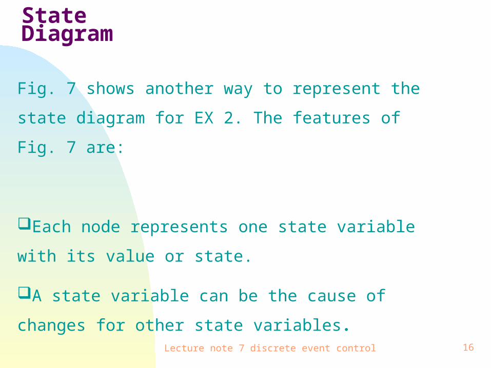
Fig. 7 shows another way to represent the state diagram
for EX 2. The features of Fig. 7 are:
Each node represents one state variable with its value or
state.
A state variable can be the cause of changes for other
state variables.

Lecture note 7 discrete event control 17
State Diagram
Fig. 7
Remark:
The meaning that the pump can never be on if the valve is closed is not represented by the state diagram.
This shows a limitation of the state diagram

Lecture note 7 discrete event control 18
State Diagram
Control system(X: state variable)
Level of fluid: LLS
X1: state variable: pump
X2: state variable: valve
Output (for controller): X1, X2
So we have: output = state variable
Lecture note 7 discrete event control 19
State Diagram: Summary
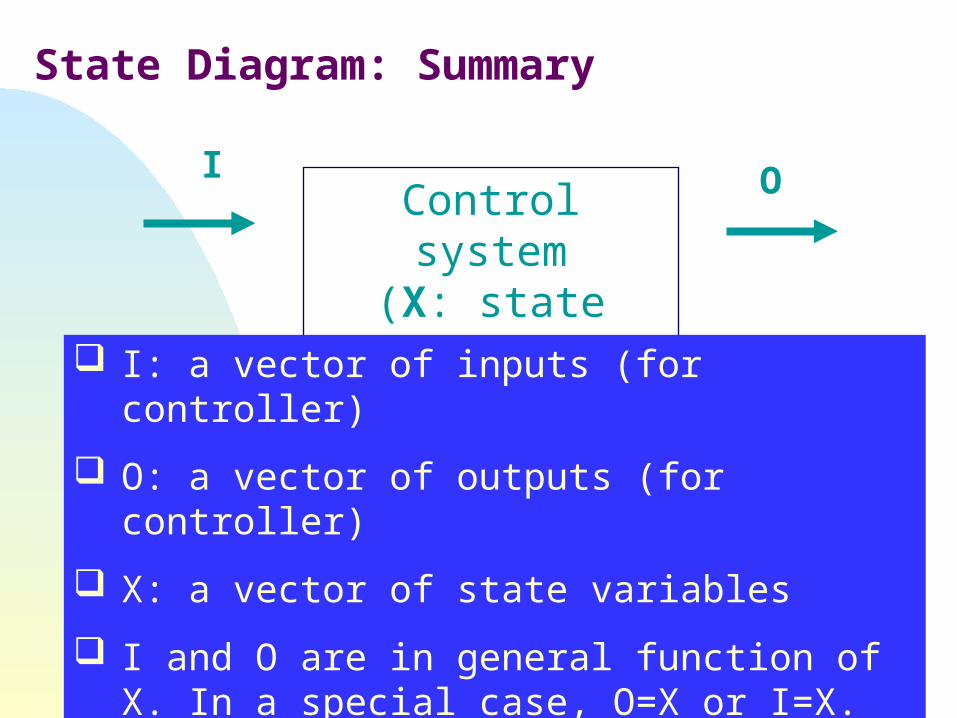
Control system(X: state variable)
I
I: a vector of inputs (for controller)
O: a vector of outputs (for controller)
X: a vector of state variables
I and O are in general function of X. In a special case, O=X or I=X.
O
Lecture note 7 discrete event control 20
State Diagram: Summary
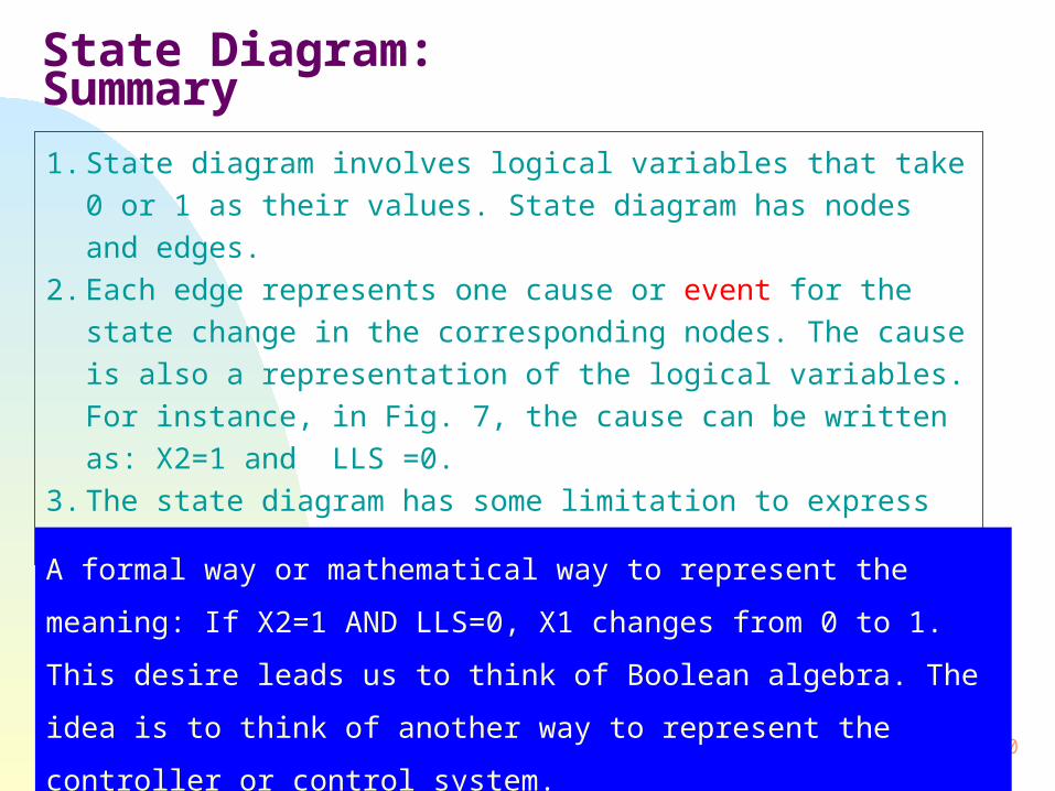
1. State diagram involves logical variables that take 0 or 1 as their values. State diagram has nodes and edges.
2. Each edge represents one cause or event for the state change in the corresponding nodes. The cause is also a representation of the logical variables. For instance, in Fig. 7, the cause can be written as: X2=1 and LLS =0.
3. The state diagram has some limitation to express the meaning of the desired control action.
A formal way or mathematical way to represent the meaning: If
X2=1 AND LLS=0, X1 changes from 0 to 1. This desire leads us
to think of Boolean algebra. The idea is to think of another way
to represent the controller or control system.
Lecture note 7 discrete event control 21
Boolean Logic Equations
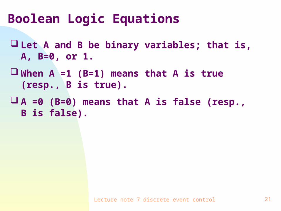
Let A and B be binary variables; that is, A, B=0, or 1.
When A =1 (B=1) means that A is true (resp., B is true).
A =0 (B=0) means that A is false (resp., B is false).

Lecture note 7 discrete event control 22
Boolean Logic Equation – operational property
1. A+B means that either A or B is true. Examples: A+B=0 when A=0 and B=0. A+B=1 otherwise.
2. AB means that both A and B are true. Examples: AB=1 when A=1 and B=1. AB=0 otherwise.
3. Not operation, by A
1A
0A
when A=0
when A=1


![Defense-related Applications of Discrete Event Simulation · Defense-related Applications of Discrete Event Simulation. ... [Banks, 2010] Defense-related ... • Randomness in discrete](https://static.fdocuments.net/doc/165x107/5ae74c3d7f8b9a6d4f8dde4b/defense-related-applications-of-discrete-event-simulation-applications-of-discrete.jpg)
