Lecture 9 Signal Noise SlidesDas

8/13/2019 Lecture 9 Signal Noise SlidesDas

http://slidepdf.com/reader/full/lecture-9-signal-noise-slidesdas 1/32

CE304-DC603 Slides

LECTURE 9:

NOISE IN

CONTINUOUS-WAVE

MODULATION SYSTEMS

Dr. N. Das and A/Prof Zhuquan Zang

Dept of Electrical and Computer

Engineering

Curtin UniversityPerth, Western Australia

Semester 2, 2012 0



CE304-DC603 Slides

LECTURE 9: NOISE INCONTINUOUS-WAVE

MODULATION SYSTEMS

In performing the noise analysis of a communica-

tion system, the customary practice is to assume

that the noise n(t) is additive, white and Gaus-

sian noise (AWGN ).

Let the double-sideband power spectral density

(PSD) S n(f ) of n(t) be N o/2, as shown below:

Semester 2, 2012 1



CE304-DC603 Slides

Note:

N o is the average noise power per unit bandwidthmeasured at the front end of the receiver, which

has a bandwidth of 2B Hz centered at the fre-quency f c.

With f c >> 2B, the narrowband noise can berepresented as

n(t) = nI

(t) cos(2πf ct)−

nQ

(t) sin(2πf ct)

where nI (t) is the in-phase and nQ(t) the quadra-ture noise component, both measured with re-spect to the carrier frequency f c.

The PSD of nI (t) and nQ(t) is

S nI (f ) = S nQ(f ) =

S n(f + f c) + S n(f − f c) |f | ≤ B0, |f | > B

=

N 0

2 + N 0

2 = N 0 |f | ≤ B

0, |f | > B

Semester 2, 2012 2



CE304-DC603 Slides

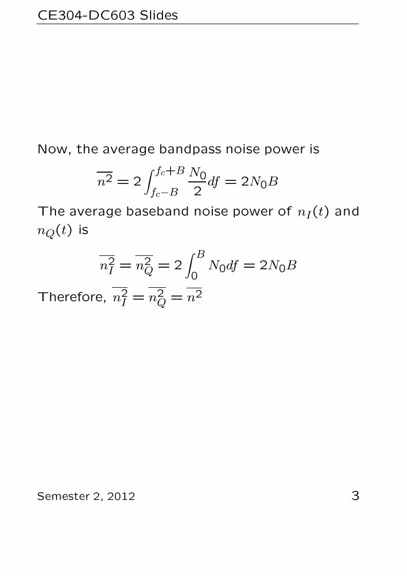
Now, the average bandpass noise power is

n2 = 2 f c+B

f c−

B

N 02

df = 2N 0B

The average baseband noise power of nI (t) and

nQ(t) is

n2I = n2

Q = 2 B

0N 0df = 2N 0B

Therefore, n2

I = n2

Q = n2

Semester 2, 2012 3



CE304-DC603 Slides

Noise in DSB-SC-AM Receivers

A double sideband suppressed-carrier amplitude-

modulated (DSB − SC − AM ) signal c(t) is rep-

resented by

c(t) = Acm(t) cos(2πf ct)

where Ac is the carrier amplitude, and m(t) is the

modulating signal with a bandwidth of B Hz.

White Gaussian noise n(t) (e.g., arising from the

front end stages of the receiver) is added to the

received signal c(t), and the resultant compos-ite signal of [c(t) + n(t)] is then detected by a

coherent product demodulator as shown:

Semester 2, 2012 4



CE304-DC603 Slides

The input to the product demodulator is

vi(t) = c(t) + n(t) =

= Acm(t) cos(2πf ct) + nI (t) cos(2πf ct) −− nQ(t) sin(2πf ct) =

= [Acm(t) + nI (t)] cos(2πf ct) − nQ(t) sin(2πf c

The local carrier ν L(t) is assumed phase-locked

to the transmitted carrier, i.e.,

ν L(t) = cos(2πf ct)

.

Therefore, the output of the demodulator is given

by

vo(t) = vi(t) × vL(t)

= [Acm(t) + nI (t)] cos2(2πf ct)−− nQ(t) sin(2πf ct) cos(2πf ct)

= [Acm(t) + nI (t)]12[1 + cos(4πf ct)]−

−1

2nQ(t) sin(4πf ct)= [Acm(t)+nI (t)]

2 + 12{[Acm(t) + nI (t)] cos(4πf c

− nQ(t) sin(4πf ct)}.

Semester 2, 2012 5



CE304-DC603 Slides

After lowpass filtering by LPF, the demodulated

output becomes

vo(t) = k[Acm(t) + nI (t)]

where k is an amplitude constant.

Now, the performance of a demodulator is de-

termined by comparing its output signal-to-noise

power ratio (SNR o) with is input signal-to-noise

power ratio (SNR I ).

Semester 2, 2012 6



CE304-DC603 Slides

(i) Determination of SNRI

The input modulated carrier power is given by

P si = limT →∞

12T

T −T c2(t)dt =

= limT →∞

12T

T −T A2

c m2(t)2 [1 + cos(4πf ct)]dt =

= limT →∞

12T

T −T A2

c m2(t)2 dt = P cP m

where P c = A2c /2 is the carrier power, and P m is

the average power of m(t).

The input noise power is

P ni = limT →∞

1

2T

T

−T n2(t)dt = 2

f c+B

f c−B

N o

2 df = 2N oB

where N o/2 is the double-sideband power spec-

tral density of n(t).

The signal-to-noise ratio at the input of the de-

modulator is given by

SN RI = P si

P ni=

P cP m

2N oB.

Semester 2, 2012 7



CE304-DC603 Slides

(ii) Determination of SNRo

The output signal power is given by

P so = limT →∞

12T

T

−T [kAcm(t)]2dt = 2k2P cP m,

and the output noise power is given by

P no = limT −∞

1

2T

T

−T

[knI (t)]2dt = k2

×2

B

0

N odf = k2

×

The signal-to-noise ratio at the output of

the demodulator is

SN Ro = P so

P no

= 2k2P cP m

2k2

N oB

= P cP m

N oB

.

Therefore, SN Ro = 2 × SN RI or

SN Ro(dB) = SN RI (dB) + 3dB.

Note: The coherent demodulation of DSB-SC-AM signal achieves a 3dB improvement in the

output signal-to-noise power ratio at the expense

of requiring twice the baseband bandwidth for its

transmission.

Semester 2, 2012 8



CE304-DC603 Slides

Envelope Detector in the Presence of Noise

An envelope detector is commonly used to de-

modulate a DSB-AM signal represented by

c(t) = [m(t) + Ac] cos(2πf ct)

where Ac and f c are the carrier amplitude and fre-

quency, respectively, and m(t) is the modulatingsignal of bandwidth B Hz and |m(t)|≤Ac.

The received DSB-AM signal c(t) is corrupted

by white Gaussian noise n(t) as shown below:

The input to the envelope detector is given by

vi(t) = c(t) + n(t) == [m(t) + Ac] cos(2πf ct) + nI (t) cos(2πf ct)−− nQ(t) sin(2πf ct).

Semester 2, 2012 9



CE304-DC603 Slides

Now, rewrite nI (t) = x, nQ(t) = y, and m(t) =

m, then

vi(t) = [m + Ac + x] cos(2πf ct) − y sin(2πf ct).

This can be expressed in the polar form, such

that

vi(t) = e(t) · cos[2πf ct + ϕ(t)]

where e(t) ≡ envelope of v i(t) = [(m+Ac +x)2+

y2]12,

and ϕ(t) = tan−

1 y

m+Ac+x.

The envelope detector extracts e(t) out from

v i(t), and after lowpass filtering by LPF, the out-

put becomes

vo(t) = e(t) = [(m + Ac + x)2 + y2]12

= [A2c + m2 + x2 + y2 + 2Acx + 2Acm + 2mx]

Semester 2, 2012 10



CE304-DC603 Slides

To simplify the analysis, consider the followingtwo extreme conditions:

(i) Input carrier-to-noise ratio CNR I is very large,i.e., Ac>>x, and y , and that the modulationindex is small, i.e., Ac>>m.

(ii) CNR I being very small, i.e., Ac<<x , and y .

Condition (i) Rewrite v o(t), such that

vo(t) = Ac

1 +

m

Ac

2

+

x

Ac

2

+

y

Ac

2

+ 2m

Ac+

2x

Ac+

2mx

A2c

Since Ac>>x , and y , and also Ac>>m, then v o(t)

can be approximated by

vo(t) ∼= Ac

1 +

2(m + x)

Ac

12

.

Applying the Binomial expansion,

vo(t) = Ac

1 + 1

22(m+x)

Ac +

12

12−1

2!

2(m+x)

Ac

2+ ...

= Ac

1 + (m+x)

Ac − 1

4

m+x

Ac

2+ ...

∼= Ac + m + x ≡ [Ac + m(t)] + nI (t).

Semester 2, 2012 11



CE304-DC603 Slides

Note:

Under very good CNR i, the output v o(t) of the

envelope detector is the same as that of the

product demodulator.

Condition (ii)

Rewrite v o(t) in the form

vo(t) = (x2 + y2)12

1 +

A2c +m2+2Acm+2x(Ac+m)

x2+y2

12

≡ (x2 + y2)12[1 + z]

12.

Under the condition of low CNR I , z <1, and using

Binomial expansion,

vo(t) ∼= (x2 + y2)12

1 + 1

2z + ...

= (x2 + y2)12 +

A2c +m2+2Acm+2x(Ac+m)

2(x2+y2)12

.

Note that under the condition of low CNR I , v o(t)

does not contain the modulating signal m(t) ex-

plicitely. It can be shown that as the CNR I falls

Semester 2, 2012 12



CE304-DC603 Slides

below about 10 dB , the performance of the en-

velope detector begins to deteriorate rapidly, in-dicating the presence of threshold effect.

Note: The actual location of the threshold de-

pends on the diode law.

There is no threshold effect with the product

demodulator.

Semester 2, 2012 13



CE304-DC603 Slides

DSB-SC-AM versus DSB-AM

The product demodulator can be used for de-

tecting both DSB-SC-AM and DB-AM signals,

while the envelope detector is only applicable for

DSB-AM.

If a product demodulator is used, then for equal

average power in the sidebands for both the DSB-

SC-AM and DSB-AM signals, the output SNR

will be the same in both cases, i.e., SNRo =2SN RI .

Now, for a given average power of the transmit-

ter, the carrier power present in the DSB-AM

signal will help to increase the sideband power in

DSB-SC-AM.

For example, the voltage spectrum of a DSB-AM

signal for modulation index M=1 is as shown:

Semester 2, 2012 14



CE304-DC603 Slides

The total transmitted power

P t = Ac

4√ 22

+ Ac

4√ 22

+ Ac

2√ 22

=

3A2c

16

The transmitted sideband power with DSB-AM

is

P DSB

−AM =

Ac

4√ 22

+ Ac

4√ 22

= A2

c

16

.

The transmitted sideband power with DSB-SC-

AM is

P DSB−SC −AM = P t = 3A2

c

16 .

Under this condition,i.e., M=1, the resulting out-

put SNR will be

SN Ro(DSB−SC −AM ) = 3 × SN Ro(DSB−AM ).

Note:

The gain in SNR for DSB-SC-AM is even greater

for smaller values of modulation index M .

Semester 2, 2012 15



CE304-DC603 Slides

Noise performance of a frequency discrimi-

nator

For noise analysis, the frequency discriminator is

modelled as a phase detector (PD) followed by

a differentiator.

A frequency-modulated (FM) signal is represented

as

c(t) = Ac cos[2πf ct + φc(t)]

where Ac and f c are the carrier amplitude and fre-

quency,respectively, and the information bearingphase function is given by

φc(t) = kf

t

−∞m(τ )dτ

Semester 2, 2012 16



CE304-DC603 Slides

where m(t) is the modulating signal, and k f is

the modulator constant.

A frequency discriminator extracts from c(t) the

differential phase term, i.e., d[φc(t)]dt .

The predetection bandpass filter BPF has a band-

width of B Hz (usually determined using the Car-

son’s rule) for minimising noise.

At the output of BPF, the bandlimited noise isrepresented by its quadrature components, such

that

n(t) = nI (t) cos(2πf ct) − nQ(t) sin(2πf ct)

where nI (t) and nQ(t) are white Gaussian noisewaves of power P n and bandwidth B/2.

Semester 2, 2012 17



CE304-DC603 Slides

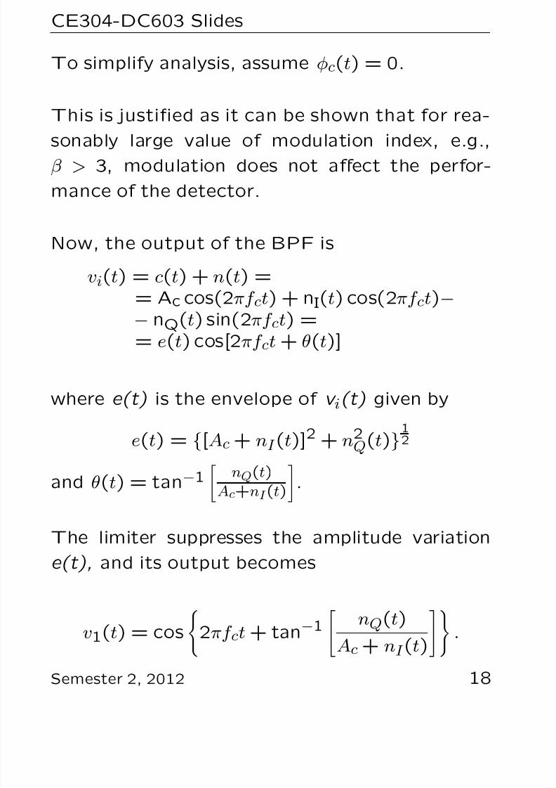
To simplify analysis, assume φc(t) = 0.

This is justified as it can be shown that for rea-

sonably large value of modulation index, e.g.,β > 3, modulation does not affect the perfor-

mance of the detector.

Now, the output of the BPF is

vi(t) = c(t) + n(t) == Ac cos(2πf ct) + nI(t) cos(2πf ct)−− nQ(t) sin(2πf ct) == e(t) cos[2πf ct + θ(t)]

where e(t) is the envelope of v i(t) given by

e(t) = {[Ac + nI (t)]2 + n2Q(t)}1

2

and θ(t) = tan−1

nQ(t)

Ac+nI (t)

.

The limiter suppresses the amplitude variation

e(t), and its output becomes

v1(t) = cos

2πf ct + tan−1

nQ(t)

Ac + nI (t)

.

Semester 2, 2012 18



CE304-DC603 Slides

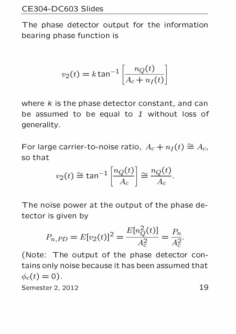
The phase detector output for the information

bearing phase function is

v2(t) = k tan−1

nQ(t)

Ac + nI (t)

where k is the phase detector constant, and can

be assumed to be equal to 1 without loss of generality.

For large carrier-to-noise ratio, Ac + nI (t) ∼= Ac,

so that

v2(t) ∼= tan−1n

Q(t)

Ac

∼= nQ

(t)

Ac.

The noise power at the output of the phase de-

tector is given by

P n,PD = E [v2(t)]2 = E [n

2

Q(t)]A2

c= P n

A2c

.

(Note: The output of the phase detector con-

tains only noise because it has been assumed that

φc(t) = 0).

Semester 2, 2012 19



CE304-DC603 Slides

Since nQ(t) is white and Gaussian, then the power

spectral density (PSD) of the noise at the out-

put of the phase detector is also white as given

by

P SDP D = P n,PD

B =

P n

A2c B

.

Now, for the frequency discriminator (FD), the

output of the phase detector is differentiated.

The transfer function of a differentiator is given

by

H (f ) = j2πf.

Therefore, the PSD of the noise at the output

of a frequency discriminator is

P SDF D = |H (f )|2 · P SDP D =

=

4π2f 2P n

A2c B

for

−B2 ≤

f

≤ B

2

0 elsewhere.

Note that the PSD of noise at the output of a

frequency discriminator is parabolic.

Semester 2, 2012 20



CE304-DC603 Slides

The noise power at the output of the lowpassfilter LPF, assumed ideal with a bandwidth of f m, is

P no = f m

−f mP SDF Ddf =

f m

−f m

4π2f 2P n

A2c B

df = 8π2f 3mP n

3A2c B

.

To determine the signal power, it is customaryto assume that the modulating signal m(t) is si-

nusoidal of frequency f m, such thatm(t) = Am cos(2πf mt).

Further, assume that this modulating signal m(t)yields a peak frequency deviation ∆f .

Semester 2, 2012 21



CE304-DC603 Slides

If the phase detector constant is 1 volt/radian,

and the differentiator giving an output of 1 volt

per volt/sec , the same assumptions as adopted

for the noise calculations, then the frequency dis-criminator constant becomes 2π volt/Hz.

Hence, the signal amplitude at the output of the

frequency discriminator is 2π∆f volts, and the

signal power is

P s,FD =

2π∆f √

2

2

= 2π2∆f 2.

The signal-to-noise ratio at the output of the

frequency discriminator becomes

SNRo = P s,FD

P no=

2π2∆f 2

8π2f 3mP n3A2

c B

=

= 3A2

cB∆f 2

4f 3mP n = 3∆f 3

f 3m

Ac√ 2

2

P n = 3β3 · SN RI

where B = 2∆f , and the modulation index β =∆f f m

.

Semester 2, 2012 22



CE304-DC603 Slides

Express in decibel, the output signal-to-noise

ratio is

SN Ro(dB) = SN RI (dB)+30log10(β) + 4.77 dB.

Notes:

• The improvement in output signal-to-noise

ratio for FM is achieved at the expense intransmission bandwidth which increases with

modulation index β.

• The above analysis assumes a sinusoidal mod-

ulating signal yielding a peak deviation ∆f .However, for a noise-like modulating signal

yielding the same frequency deviation, its mean

square amplitude or power is only 2/9 time

that of a sinusoidal signal. This corresponds

to a decrease of about 6.5 dB in SNR o for

noise-like modulating signal.

• The SN Ro obtained from the above analysis

is reasonably accurate for β ∼= 3. For smaller

Semester 2, 2012 23



CE304-DC603 Slides

values of β, FM becomes quasi-linear, i.e.,

narrowband FM, and its performance then

approaches that of DSB-SC-AM demodulated

using a coherent product demodulator.

• The above performance analysis assumes the

input carrier-to-noise ratio CNR I is high. The

analysis for low CNR I is very difficult. At low

values of CNR I , the noise amplitude is suf-ficiently large to cause the addition or dele-

tion of a pair of zero crossings to be inserted

into the detected carrier. This gives rise to

positive or negative impulse of area 2 π radi-

ans depending whether an extra cycle having

been slipped in or deleted. The effect is sig-

nificant deterioration in SNR o.

It has been shown that as the CNR I falls, the

number of impulses per second increases as

given by

No. of impulses/sec ≈ exp(−SN RI )

2 m(t).

For a frequency discriminator, this effect oc-

curs at an CNR I value of about 10 dB , which

Semester 2, 2012 24



CE304-DC603 Slides

is normally taken as the threshold of the dis-

criminator.

• A phase-locked loop exhibits a much lower

impulse rate than a conventional frequency

discriminator. Consequently, the threshold

of a PLL FM demodulator can be up to 10 dB lower than a conventional frequency dis-

criminator.

Semester 2, 2012 25



CE304-DC603 Slides

Noise performance of the FM discriminator

Semester 2, 2012 26



CE304-DC603 Slides

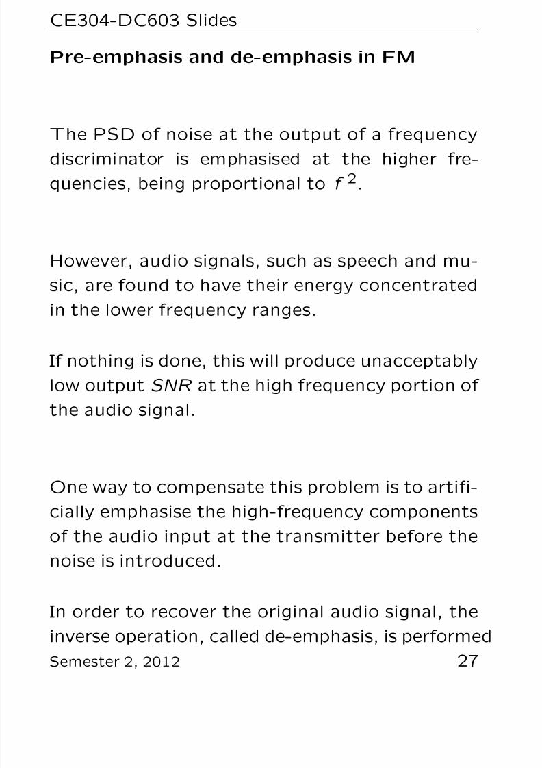
Pre-emphasis and de-emphasis in FM

The PSD of noise at the output of a frequencydiscriminator is emphasised at the higher fre-

quencies, being proportional to f 2.

However, audio signals, such as speech and mu-sic, are found to have their energy concentrated

in the lower frequency ranges.

If nothing is done, this will produce unacceptably

low output SNR at the high frequency portion of

the audio signal.

One way to compensate this problem is to artifi-

cially emphasise the high-frequency components

of the audio input at the transmitter before thenoise is introduced.

In order to recover the original audio signal, the

inverse operation, called de-emphasis, is performed

Semester 2, 2012 27



CE304-DC603 Slides

at the output of the frequency discriminator in

the receiver.

Further, in this de-emphasis process, the high-

frequency components of noise are being reduced.

Pre-emphasis

A transfer function suitable for emphasising hf

components is given by

H e(f ) = 1 + j f

f o

where f o is the break frequency above which the

components are emphasised.

In practice, H e(f) is approximated by a simple

RC network:

Semester 2, 2012 28



CE304-DC603 Slides

This network has two break frequencies, f 1 and

f 2 given by

f 1 = 1

2πR1C

and f 2 ∼= 1

2πR2C with R 1>>R 2.

For broadcast FM, R 1C=75 µsec , so that f 1=2.1kHz .

The second break frequency f 2 is introduced to

prevent emphasising frequency components higher

than the audio range.

For this reason, f 2 is normally chosen to be f 2 ≤30 kHz .

Semester 2, 2012 29



CE304-DC603 Slides

De-emphasis

The de-emphasis network, following the frequency

discriminator, must have an inverse characteris-tic given by

H d(f ) = 1

1 + j f f o

.

The transfer function H d(f) can be realised usinga simple RC-network:

The break frequency f 1 = 12πC R = 2.1kH z, with

CR=75 µsec for broadcast FM.

The noise power after de-emphasis is given by

P no,d = f m−f m

P SDF D|H d(f )|2df

= f m−f m

4π2f 2P nA2

c B1

1+4π2C 2R2df .

Semester 2, 2012 30



CE304-DC603 Slides

The decrease in noise power with de-emphasis

as compared to the case with no de-emphasis

corresponds to the improvement in output SNR .

With CR=75 µsec , and f m=15 kHz , an improve-

ment in output SNR of 13 dB (or 20 times) is

achieved using pre-emphasis and de-emphasis in

FM.

Lecture 9 Signal Noise SlidesDas

Documents

Transcript of Lecture 9 Signal Noise SlidesDas