Lecture 9 Iterative control...

Lecture 9Iterative control

approaches

Modeling meets control meet modeling meets control meets modeling meets control meets modeling ...

Tuesday, April 3, 2012

Approximate System Identification & ControlMAE283B Lecture 9, Slide

An archetypeOur overall aim is to minimize a performance function on the true system

Define “local” criterion

Look at the recursion

This is a descent procedure, where each modeling and control design phase drives down the value of the local criterion, which trades nominal performance against stability robustness

This particular approach is infeasible because it requires knowledge of the true plant

So we try an approximate approach using instead of Then the identification uses closed-loop data

2

Jlocal = J(G0, Gθ, C) =

��(G0 −Gθ)

C

1+GθCWH0

1+GθC

��∞

Jglobal = J(G0, C) =

��WH0

1 +G0C

��∞

Ci = argminC

Jlocal(G0, Gθ,i, C)

Gθ,i+1 = argminθ

Jlocal(G0, Gθ, Ci)

H2 H∞



Hakvoort and the Dutch mastersFix the control design method .... LQG or minimum variance

Adjust the identification noise model iteratively, and based on the current plant model, to create a control-relevant criterion via the noise model

Rinse and repeatThe aim is to prefilter the prediction error to yield the optimal data properties associated with identifying a model for subsequent LQG control design - a theory developed by Gevers and Ljung for the case of the system being in the model set. The optimal identification conditions occur when the system is optimally controlled.This indirect approach works in examples but is not theoretically fully supported ... nor is any other scheme

3

Hf = (1 +GθC)



The windsurfer scheme

An approach of increasing performanceStep 1: excite two closed loops, one with the real plant and the designed closed loop with the model. Determine satisfaction with modeling performance

happy: move to Step 2sad: identify a new model using Hansen scheme

based on coprime factor methods, control-relevantStep 2: design a new feedback controller using Internal Model Control with larger bandwidth, go to Step 1

applicable for stable plants, closed-loop bandwidth is a parameter

Step 2A: use control-oriented model reduction as possible

4Tuesday, April 3, 2012


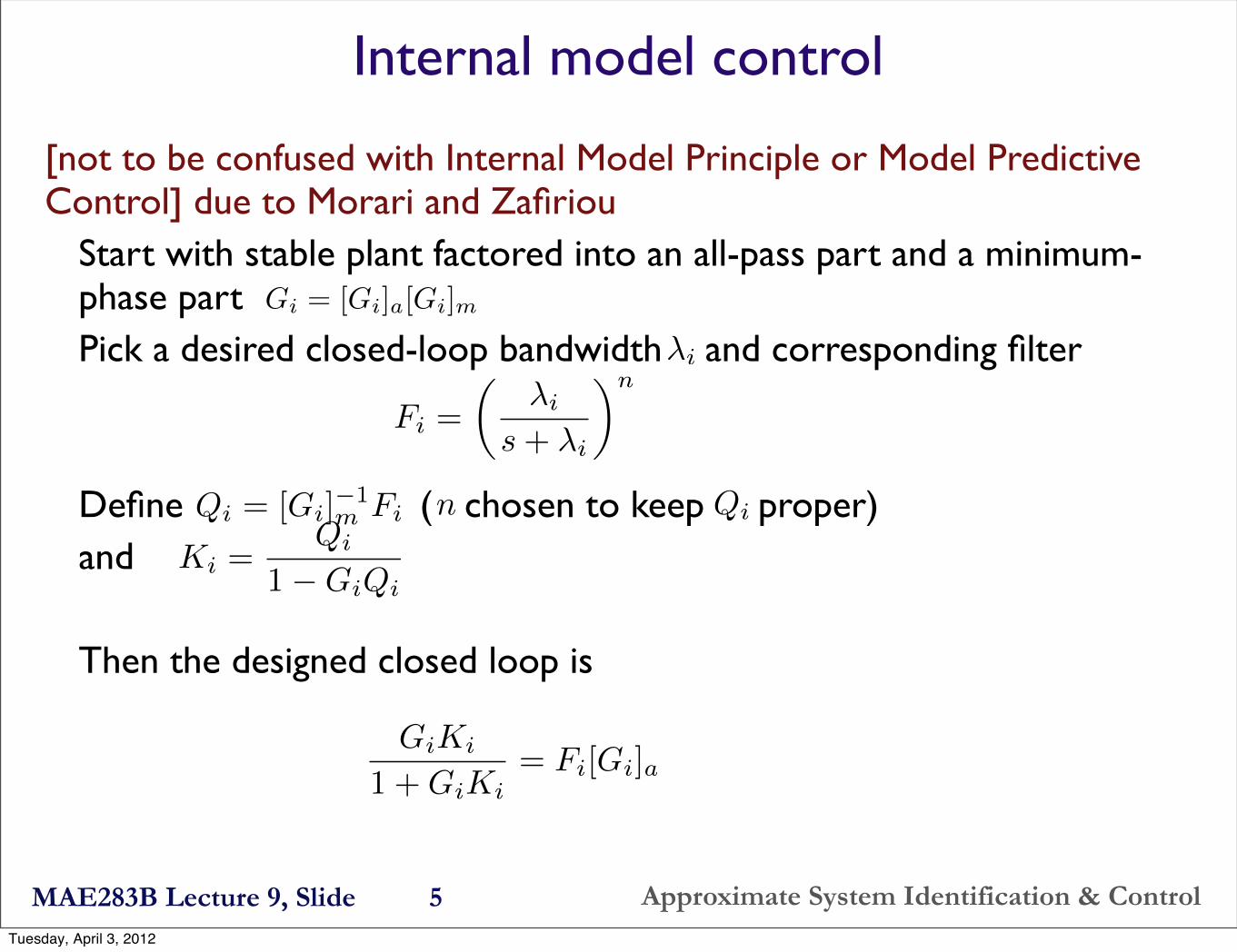
Internal model control

[not to be confused with Internal Model Principle or Model Predictive Control] due to Morari and Zafiriou

Start with stable plant factored into an all-pass part and a minimum-phase partPick a desired closed-loop bandwidth and corresponding filter

Define ( chosen to keep proper) and

Then the designed closed loop is

5

Gi = [Gi]a[Gi]m

Fi =

�λi

s+ λi

�nλi

Qi = [Gi]−1m Fi

Ki =Qi

1−GiQi

GiKi

1 +GiKi= Fi[Gi]a

n Qi



Coprime factor identification

6

C G0

rt ut yt

vt

−+ +

Assume we have a stable closed loop with the real plantSuppose we know another plant model which is stabilized by

Then we may write coprime factor descriptions of and

where the factors are stable proper transfer functionWithout loss of generality we can assume

Since is also stabilized by , it can be written for some stable proper transfer function

Let’s try to estimate

G0

G C

CG

G =N

DC =

X

Y

NX +DY = 1

C

G0

R

R

G0 =N +RY

D −RX



Coprime factor identification

Hansen, Franklin and Kosut noted the followingCreate signals and

[simple algebra yields this relation]Now fit the Youla-Kucera parameter transfer function and the noise model by minimizing the filtered prediction error

Filtered reference and data signals yield independentFreedom from bias, control-relevant

7

G =N

DC =

X

YG0 =

N +RY

D −RXKnown Find

αt = Xrt βt = Dyt −Nut

= Rαt + (D −RX)Het

Rθ

εfθ,t = Y (βt −Rθαt)

=

�G0C

1−G0C− GC

1 +GC

�rt +

1

1 +G0CH0et

(αt,βt)



The Zang scheme

Control design

then use the frequency-weighting trick from last lecture

HopefullyIntersperse with control-relevant modeling

based on minimizing the second term using closed-loop data and data filter

8

Jglobal(G0, C) = limN→∞

1

N

N�

t=1

y2t+ γu

2t=

��

H01+G0C

γ1/2 C

1+G0CH0

��2

Jlocal(Gθ, C) = limN→∞

1

N

N�

t=1

y2t+ γu

2t=

��

Hθ1+GθC

γ1/2 C

1+GθCHθ

��2

JF

local(Gθ, C) = limN→∞

1

N

N�

t=1

(Fy)2t+ γ(Fu)2

t=

��

HθF

1+GθC

γ1/2 C

1+GθCHθF

��2

JFlocal(Gθ, C) → Jglobal(G0, C)

��

H01+G0C

γ1/2 C

1+G0CH0

��2

≤

��

Hθ1+GθC

γ1/2 C

1+GθCHθ

��2

+

��

�H0

1+G0C

γ1/2 C

1+G0CH0

�−�

Hθ1+GθC

γ1/2 C

1+GθCHθ

��2

|Lθ|2 = (1 + γ|C|2)��

Hθ

1 +GθC

��2



References

Pedro Albertos & Antonio Sala, Iterative Identification & Control, Springer 2002

Chapters on Windsurfer & Zang schemes,control-relevant identification, sugar mill, CD player, wafer stepper applications

Hakvoort, Schrama & Van den Hof, “Approximate identification with closed-loop performance criterion and application to LQG feedback design,” Automatica, vol. 30, pp. 679-690, 1994

Gevers & Ljung, “Optimal experiment designs with respect to the intended model application,” Automatica, vol. 22, pp. 543-554, 1986

Zang, Bitmead & Gevers, “Iterative weighted least-squares identification and weighted LQG control design,” Automatica, vol. 31, pp.1577-1594

Lee, Anderson, Kosut & Mareels, “A new approach to adaptive robust control,” International Journal of Adaptive Control & Signal Processing, vol. 7, pp. 183-211, 1993

Schrama, “Accurate identification for control: the necessity of an iterative scheme,” IEEE Transactions on Automatic Control, vol 37, pp.991-994, 1992



Local time-line1986 - Michel Gevers at the Australian National University

Review of Clarke, Mohtadi & Tuffs GPC papers

1988 - Bob on sabbatical at University of Louvain, Belgium, visits to Van den Hof, Schrama, Hakvoort in Delft

Draft of book “Adaptive Optimal Control: the Thinking Man’s GPC”

1989 - Started working with CSR Sugar at Victoria Mill

1990 - The George Polya moment

1990 - The Thinking Man’s book appears

1990/1 - Ari Partanen employed at Victoria Mill

1991 - First European Control Conference Grenoble. Bitmead & Zang “An iterative identification and control strategy”

Train ride (pre-TGV) from Grenoble to Brussels with Michel Gevers

20-page fax to Zhuquan Zang

Discussions with Robert Kosut, co-editor of IEEE Trans AC special issue

1993 - Ari comes to ANU as a PhD student ... still has the passwords to CSR computers, experiments on the sugar mill

1993 - Raymond de Callafon, Paul Van den Hof and Okko Bosgra experiment on iterative identification and control on Philips CD player and ASML wafer stepper

1995 - Iterative Feedback Tuning ideas appear

1995 - Zang (theory) and Ari (application) papers appear in the same issue of Automatica

1999 - Pedro Albertos arranges a workshop in Valencia

Leads to publication of the book “Iterative identification and control” 2002

1999 + - Lots of good work by Anderson, Gevers, Kosut, etc on cautious control


Lecture 9 Iterative control...

Documents

Transcript of Lecture 9 Iterative control...